Koopman Reduced Order Modeling with Confidence Bounds

Abstract

This paper introduces a reduced order modeling technique based on Koopman operator theory that gives confidence bounds on the model’s predictions. It is based on a data-driven spectral decomposition of said operator. The reduced order model is constructed using a finite number of Koopman eigenvalues and modes while the rest of spectrum is treated as a noise process. This noise process is used to extract the confidence bounds. Additionally, we propose a heuristic algorithm to choose the number of deterministic modes to keep in the model. We assume Gaussian observational noise in our models. As the number of modes used for the reduced order model increases, we approach a deterministic plus Gaussian noise model. The Gaussian-ity of the noise can be measured via a Shapiro-Wilk test. As the number of modes increase, the modal noise better approximates a Gaussian distribution. As the number of modes increases past the threshold, the standard deviation of the modal distribution decreases rapidly. This allows us to propose a heuristic algorithm for choosing the number of deterministic modes to keep for the model.

47B33, 15A18, 62F25, 62M20

1 Introduction

The goal of reduced order modeling (ROM) is to replace a computationally intensive model (e.g., an Agent-based model) with a surrogate model that takes less computationally-expensive resources to execute. Ideally, we want to determine a computationally cheap model that is accurate within the bounds the practitioner cares about. By the inherent nature of these reduced-order models, the accuracy of the ROM degrades as we increase the parsimony of the learned model. Our goal in this paper is to develop ROM’s directly from data that also give bounds on the confidence of their predictions. Instead of the classical point estimate of the forecast of the ROM, we also get a confidence region that the true data should lie in.

Data-driven identification of a model can take many different forms. The SINDy [3] algorithm requires an a priori choice of basis, e.g. the monomials or the rational functions. This dictionary is then used to construct an ODE (or PDE) using a least squares regression. While this gives a generative model learned from the data, which can give point predictions of future values, there does not seem to be a method giving confidence bounds on these point predictions. Alternatively, the Bayesian system identification [9] formulates the problem as a hidden Markov model and claims to subsume the classical dynamic mode decomposition (DMD) and sparse DMD in its formulation [9].

Gerlach et. al. [10] use the adjoint relation between the Koopman operator and Perron-Frobenius operator to compute quantities of interest in the future. The focus is to compute the expectation of quantity of interest due to the propagation of an uncertain quantity (parametric and/or initial conditions). If given a density, $f:X\to\mathbb{R}$, representing the uncertainty in parameters or initial conditions, its propagation, under a dynamical system $S:X\to X$, is given by the Perron-Frobenius operator $P_{S}$. The expected value of a quantity $g:X\to\mathbb{R}$ at the future time is given by $\mathbb{E}[g[X]:X\sim P_{S}f]=\langle P_{S}f\,,\,g\rangle=\int(P_{S}f)(x)g(x)dx$. However, computing $P_{S}f$ requires knowledge of the pre-image map $S^{-1}:X\to X$ which is either computationally expensive or intractable, especially in the case of black-box systems. Using the adjoint relation between the Perron-Frobenius operator and the Koopman operator, $\langle P_{S}f\,,\,g\rangle=\langle f\,,\,U_{S}g\rangle$, allows one to compute the expectation of $g$ by using the Koopman operator $U_{S}g(x)=g(S(x))$. The computation of $g$ and $S$ is much cheaper than computing the pre-image map.

In [14], the authors define a Koopman operator over a Gaussian process $\mathsf{GP}(\mu,k)$. The Gaussian process is an infinite-dimensional distribution over the space of real-valued functions $f:\mathbb{R}^{n}\to\mathbb{R}$. The Gaussian process is characterized by specifying, a priori, a mean $\mu:\mathbb{R}^{N}\to\mathbb{R}$ and the covariance functions $k:\mathbb{R}^{N\times N}\to\mathbb{R}$. Assuming deterministic dynamics, the authors show that if an observable is distributed according to the Gaussian process, $f\sim\mathsf{GP}(\mu,k)$, then the Koopman operator applied to $f$ is also a Gaussian process such that $U^{t}f=\mathsf{GP}(U^{t}\mu,U^{t}k)$. The limitations of this approach are that it requires the dynamics to be deterministic and the mean $\mu$ and covariances $k$ must be specified a prior rather than being learned from data.

In this paper, we build off reduced order modeling techniques using the so-called Koopman operator [12, 13, 20, 17, 15]. For any nonlinear dynamical systems, there is an associated (infinite-dimensional) linear operator that encodes the dynamics as a linear system [17, 15, 4]. This operator is called the Koopman operator. In many cases, this linear operator has a spectral expansion which decomposes the operator into the point spectrum (eigenvalues) and their associated (Koopman) modes and the continuous spectrum [17, 15, 4]. Much recent work has been done on algorithms that compute an approximation of the point spectrum of the Koopman operator [19, 18, 21, 2, 23, 11, 5, 6, 7, 8]. These methods are purely data-driven and are based off computing a spectral decomposition of the Koopman operator without requiring a concrete representation of the operator.

Classical methods of reduced order modeling using Koopman operator theory use a finite number of the Koopman eigenvalues and associated modes. However, no consideration is given toward the confidence of the ROM’s predictions. For example, if we construct a ROM with half the number of total modes, what is our confidence on the ROM’s predictions? In this paper, we develop a method, based on Koopman operator methods, that constructs a model and also gives confidence bounds on its predictions. In short, the algorithm computes a Koopman Mode Decompositions on the training data; a finite number of the modes are selected as part of the ROM; the rest of the dynamics are modeled as a noise process, splitting the part of the noise in the subspace spanned by the Koopman modes used for the ROM (called “in-plane” for short) and the part orthogonal to those modes. The in-plane noisy dynamics are used to estimate confidence bounds on the predictions.

What is new in this paper can be summarized by the following points:

1. A reduced order modeling framework based on Koopman Mode Decomposition for stochastic dynamical systems.

2. A method of providing confidence bounds on the predictions of a reduced order Koopman model based on the estimated noise distribution of the remaining parts of the dynamics.

3. A heuristic method for determining the minimum number of modes to be used for the reduced order model. The heuristic is based on the Shapiro-Wilkes hypothesis test comparing how well the empirical distribution is represented by a Gaussian distribution.

4. Applied the method to stochastic systems with changing network topology.

The rest of the paper is structured as follows. In Section 2, we develop the mathematical framework for the reduced order modeling framework with confidence bounds in the context of stochastic dynamical systems. It includes Koopman operator theory, model reduction, and forecasting statistics. Section 3 applies the methodology to a sequence of examples, two of which have dynamically changing network topology. In Section 4, we present a heuristic algorithm for choosing the number of modes for the reduced order model using a statistical test for Gaussian distributions. We conclude the paper in Section 5.

2 Main results

2.1 Koopman Operator Theory

Consider a stochastic dynamical system

(1) $$\mathbf{x}(t+1)=T(\mathbf{x}(t),\xi(t)),\quad t\in\mathbb{N}$$

where $\mathbf{x}(t)\in\Omega\subset\mathbb{R}^{d}$, $\Omega$ is a compact Riemannian manifold, and $\xi(t)$ is an IID noise process with $\xi\sim\Xi$. Let $f_{i}\in L^{2}(M,d\mathbf{x})$ for $i=1,\dots,n$ and $\mathbf{f}=(f_{1},\dots,f_{n})$. The Koopman operator induced by the stochastic dynamical system (and parameterized by the noise sequence) is denoted as $U_{\xi}f(\mathbf{x})=f(T(\mathbf{x},\xi))$. With an abuse of notation, we will denote by $U_{\xi}^{t}f_{i}(\mathbf{x})$ the composition of $f_{i}$ with the map (1) $t$-times with the that a new value for $\xi(t)$ is drawn from the distribution at each iteration; i.e.,

(2) $$U_{\xi}^{2}f_{i}(\mathbf{x})=f_{i}(T(\mathbf{x}(1),\xi(1)))=f_{i}(T(T(\mathbf{x},\xi(0)),\xi(1))).$$

Furthermore, we define $U_{\xi}\mathbf{f}(\mathbf{x})=(U_{\xi}f_{1}(\mathbf{x}),\dots,U_{\xi}f_{n}(\mathbf{x}))$. We assume there is a spectral decomposition for $U_{\xi}$ written as

(3) $$U_{\xi}^{t}f_{i}(\mathbf{x})=\sum_{j}c_{j,\xi}\lambda_{j,\xi}^{t}\phi_{j,\xi}(\mathbf{x})+\int_{\mathbb{C}}z^{t}dE_{c,\xi}(z)f_{i}(\mathbf{x}),$$

where $c_{j,\xi}\in\mathbb{C}$, $\lambda_{j,\xi}\in\mathbb{C}$ is an eigenvalue, $\phi_{j,\xi}$ is an eigenfunction, and $dE_{c,\xi}$ is a projection-valued measure corresponding to the continuous part of the spectrum. For the vector-valued observable case, we have

(4) $$U_{\xi}^{t}\mathbf{f}(\mathbf{x})=\sum_{j}\mathbf{m}_{j,\xi}\lambda_{j,\xi}^{t}\phi_{j,\xi}(\mathbf{x})+\int_{\mathbb{C}}z^{t}dE_{c,\xi}(z)\mathbf{f}(\mathbf{x}),$$

where $\mathbf{m}_{j,\xi}$ is the $j$-th Koopman mode. For the rest of the paper, we drop the subscript $\xi$ from the Koopman modes, eigenvalues, and eigenfunctions for notational simplicity.

2.2 Model reduction

Obviously, we cannot compute the infinite expansion, so we attempt to approximate the evolution of the observable due to the operator using a finite mode expansion. That is

(5) $$U_{\xi}^{t}\mathbf{f}(\mathbf{x})=\sum_{j=1}^{J}\mathbf{m}_{j}\lambda_{j}^{t}\phi_{j}(\mathbf{x})+\mathbf{r}(t),$$

where here $\mathbf{r}(t)\sim\mathfrak{R}$ is a residual sequence from the distribution $\mathfrak{R}$ (e.g. a Gaussian distribution). Additionally, we order the modes $\mathbf{m}_{j}$ according to their norm so that $\lVert\mathbf{m}_{j}\rVert\geq\lVert\mathbf{m}_{j+1}\rVert$. This implies that the modes and eigenvalues of a lower order model are subsets of those of higher order models. Note that if $T$ or any $f_{i}$ are nonlinear, then $\mathbf{r}(t)$ will not have the same distribution as $\xi(t)$. To make the notation more compact, let us write the deterministic part as

(6) $$D_{\xi}^{t}\mathbf{f}(\mathbf{x})=\sum_{j=1}^{J}\mathbf{m}_{j}\lambda_{j}^{t}\phi_{j}(\mathbf{x}).$$

So far we have split the evolution of the observable into a deterministic part and a stochastic part. Also note, that due to the truncation of the deterministic part from an infinite sum to a finite sum, the “coefficients”, $\phi_{j}(x)$, for the Koopman modes $\mathbf{m}_{j}$ may not give the optimal deterministic reconstruction of the evolution. We will come back to this when discussing algorithms to compute the decomposition.

Now we look into splitting the modal noise into a modal component and an innovation component. Let $M=\operatorname{span}\{\mathbf{m}_{1},\dots,\mathbf{m}_{J}\}$, $\mathbf{M}$ the matrix having the Koopman modes as its columns, and $P_{M}$ the orthogonal projection onto $M$. Then,

(7) $$U_{\xi}^{t}\mathbf{f}(\mathbf{x})=\underbrace{\sum_{j=1}^{J}\mathbf{m}_{j}\lambda_{j}^{t}\phi_{j}(\mathbf{x})+P_{M}\mathbf{r}(t)}_{\in M}+\underbrace{(I-P_{M})\mathbf{r}(t)}_{\text{orthogonal to $M$}}.$$

Consider the terms lying in $M$:

(8) $$\sum_{j=1}^{J}\mathbf{m}_{j}\lambda_{j}^{t}\phi_{j}(\mathbf{x})+P_{M}\mathbf{r}(t)=\mathbf{M}\begin{bmatrix}\lambda_{1}^{t}\phi_{1}(\mathbf{x})\\ \vdots\\ \lambda_{J}^{t}\phi_{J}(\mathbf{x})\end{bmatrix}+\mathbf{M}\mathbf{M}^{+}\mathbf{r}(t)=\mathbf{M}\left(\begin{bmatrix}\lambda_{1}^{t}\phi_{1}(\mathbf{x})\\ \vdots\\ \lambda_{J}^{t}\phi_{J}(\mathbf{x})\end{bmatrix}+\mathbf{M}^{+}\mathbf{r}(t)\right),$$

where we have used the fact that $P_{M}$ can be computed as $P_{M}=\mathbf{M}\mathbf{M}^{+}$, where $\mathbf{M}^{+}$ is the Moore-Penrose pseudo-inverse of $\mathbf{M}$. We define the modal noise $\rho(t)=(\rho_{1}(t),\dots,\rho_{J}(t))^{T}$ as

(9) $$\rho(t)=\mathbf{M}\mathbf{M}^{+}\mathbf{r}(t).$$

The innovation noise is then defined as

(10) $$\eta(t)=(I-P_{M})\mathbf{r}(t)=\mathbf{r}(t)-P_{M}\mathbf{r}(t)=\mathbf{r}(t)-\rho(t).$$

The innovation noise $\eta(t)$ is orthogonal to $M$. With these definitions (7) becomes

(11) $$U_{\xi}^{t}\mathbf{f}(\mathbf{x})=\left(\mathbf{M}\begin{bmatrix}\lambda_{1}^{t}\phi_{1}(\mathbf{x})\\ \vdots\\ \lambda_{J}^{t}\phi_{J}(\mathbf{x})\end{bmatrix}+\rho(t)\right)+\eta(t).$$

2.3 Algorithm: Forecasting with confidence bounds

Given the stochastic reduced order model (11) one could compute predictions and statistics for those predictions if we knew the distributions of $\rho(t)$ and $\eta(t)$. Note that the distribution of these can be computed since these are just linear transformations of $\mathbf{r}(t)$. However, $\mathfrak{R}$ is usually unknown. Even if we had the analytic form of the distribution $\Xi$ that the noise process $\xi$ follows (see eq. (1)), an analytic form for $\mathfrak{R}$ can be very difficult to find since $\Xi$ passes through a couple of nonlinear transformations, namely $T$ and $\mathbf{f}$.

2.4 Forecasting statistics

Once the noise sequences $r(t),\rho(t),\eta(t)$ are known, probability density models need to be constructed for which drawing samples is easy, say with multivariate kernel density estimation techniques. Assume the densities for $\rho$ and $\eta$ are computed.

2.4.1 Prediction in the subspace M.

Recall that $M$ is the subspace spanned by the Koopman modes, $M=\operatorname{span}\{\mathbf{m}_{1},\dots,\mathbf{m}_{J}\}$, and $P_{M}$ is the orthogonal projection onto $M$. By (11) and since the innovation sequence $\eta$ is orthogonal to $M$ we have

(12) $$P_{M}U_{\xi}^{t}\mathbf{f}(\mathbf{x})=D_{\xi}^{t}\mathbf{f}(\mathbf{x})+\rho(t).$$

Then

(13) $$\mathbb{E}P_{M}U_{\xi}^{t}\mathbf{f}(\mathbf{x})=\mathbb{E}D_{\xi}^{t}\mathbf{f}(\mathbf{x})+\mathbb{E}\rho(t)=D^{t}\mathbf{f}(\mathbf{x})+\mathbb{E}\rho(t).$$

Thus the expected prediction in $M$ is the deterministic prediction but with a constant offset depending on the expected value of $\rho(t)$. Similarly, the variance of the predictions in the plane are

(14) $$\operatorname{Var}[P_{M}U_{\xi}^{t}\mathbf{f}(\mathbf{x})]=\mathbb{E}(P_{M}U_{\xi}^{t}\mathbf{f}(\mathbf{x})-\mathbb{E}P_{M}U_{\xi}^{t}\mathbf{f}(\mathbf{x}))^{2}=\mathbb{E}(\rho(t)-\mathbb{E}\rho(t))^{2}=\operatorname{Var}(\rho(t)).$$

Both of these results make sense since we have structured our model to have additive noise.

2.5 Algorithm

Let us assume that $\mathfrak{R}$ is not known analytically and we cannot numerically generate samples from it directly. Thus we have to estimate the distribution from the data. Algorithm 1 summarizes the basic computations for computing a reduced order model. It returns the deterministic part of the model, the residual noise sequence, the modal noise sequence, and the innovation noise sequences. We note that while we are working with i.i.d. stochastic dynamical systems, and therefore should be working with the stochastic Koopman operator [15], (15) computes the reconstruction coefficients along a single realization of evolution of the dynamical system. Wanner and Mezić [22] show the convergence of these coefficients to the true reconstruction coefficients of the stochastic Koopman operator using an ergodicity argument in the large data limit $T\to\infty$.

Algorithm 1 Koopman Reduced Order Model for Stochastic Systems (KROM)

  Input Data: $\{U_{\xi}^{t}\mathbf{f}(\mathbf{x})\}_{t=0}^{T}$ stochastic evolution of observable

  1: Compute KMD of data $\to(\{\mathbf{m}_{j}\}_{j=1}^{M},\{\lambda_{j}\}_{j=1}^{M})$.

  2: Order the Koopman modes $\{\mathbf{m}_{j}\}_{1}^{M}$ by their norm $\lVert\mathbf{m}_{j}\rVert$, where $\lVert\mathbf{m}_{j}\rVert\geq\lVert\mathbf{m}_{j+1}\rVert$.

  3: Once ordered, normalize each mode to have norm 1.

  4: Choose truncation number $J>0$ according to some criterion

  5: Compute modal reconstruction coefficients:

(15) $$\mathbf{c}=\operatorname*{arg\,min}_{\alpha\in\mathbb{C}^{n}}\sum_{t=0}^{T-1}\lVert U_{\xi}^{t}\mathbf{f}(\mathbf{x})-\sum_{j=1}^{J}\alpha_{j}\lambda_{j}^{t}\mathbf{m}_{j}\rVert_{2}^{2}.$$

  6: Construct deterministic reconstruction model with input parameter $t$ that returns

(16) $$D_{\xi}^{t}\mathbf{f}(\mathbf{x})=\sum_{j=1}^{J}c_{j}\lambda_{j}^{t}\mathbf{m}_{j}.$$

  7: Compute residual sequence

(17) $$\mathbf{r}(t)=U_{\xi}^{t}\mathbf{f}(\mathbf{x})-D_{\xi}^{t}\mathbf{f}(\mathbf{x}).$$

  8: Compute modal noise sequence

(18) $$\rho(t)=\mathbf{M}\mathbf{M}^{+}\mathbf{r}(t).$$

  9: Compute innovation sequence

(19) $$\eta(t)=\mathbf{r}(t)-\rho(t).$$

  return  $D_{\xi}^{t}\mathbf{f}(x)$, $\{\mathbf{r}(t)\}_{t=0}^{T}$, $\{\rho(t)\}_{t=0}^{T}$, $\{\eta(t)\}_{t=0}^{T}$

In Algorithm 2, we use the deterministic model and the modal noise sequence to get confidence bounds for the forecasts of the deterministic model. The idea is to estimate a Gaussian distribution for each coordinate using the modal sequence and use the standard deviations of these distributions to compute the confidence bounds. While the most common case will involve real data, we have formulated the algorithm to take in complex data. Gaussian distributions will be estimated for the real and complex parts individually. Their respective standard deviations will give confidence bounds on the real and complex parts of the deterministic model’s forecast.

Algorithm 2 KROM Forecasting with confidence bounds

  Input Data: $D_{\xi}^{t}\mathbf{f}(x)$ (deterministic model), $\{\rho(t)\}_{t=0}^{T}$ (modal sequence) where $\rho(t)\in\mathbb{C}^{n}$

  1: For each coordinate $i$ of the modal sequence, estimate a Gaussian distribution $G_{i}\in C$, where $\Re(G_{i})$, the real part of $G_{i}$ is estimated from the real part of $\rho(t)$ and similarly for the complex part.

  2: Compute $\mathbf{S}=(s_{1},\dots,s_{n})\in\mathbb{C}^{n}$, where $\Re(s_{i})$ is the standard deviation of the real part of $G_{i}$ and similarly for the complex part.

  3: For time $t\in\mathbb{N}$, compute the forecast as $\tilde{f}(t)=D_{\xi}^{t}\mathbf{f}(x)$. The confidence bounds are given $[\tilde{f}(t)-2\mathbf{S},\tilde{f}(t)+2\mathbf{S}]\in\mathbb{C}^{n\times 2}$.

3 Experimental results

In this section, the reduced order modeling algorithm and the forecasting algorithm are applied to a sequence of examples.

3.1 Linear Modal System

We first test the Koopman Reduced Order Model (KROM) method for a system with known modes and eigenvalues. The general model of the system is given by

(20) $$\mathbf{x}(t)=\left(\sum_{j=1}^{J}\mathbf{m}_{j}\lambda_{j}^{t}\right)+\xi(t)\in\mathbb{C}^{n}$$

where $\mathbf{m}_{j}\in\mathbb{R}^{n}$, $\lambda_{j}\in\mathbb{C}$, $t\in\mathbb{N}$, and $\xi(t)\in\mathbb{R}^{n}$ is a noise sequence with each coordinate independent with a normal distribution. We note that the evolution of this system is in $\mathbb{C}^{n}$ rather than $\mathbb{R}^{n}$ due to the choice of complex $\lambda_{j}$’s; therefore, there will not be complex conjugate pairs.

For the following numerical results, the system parameters were chosen as $J=20$, $n=40$, and $\xi_{i}(t)\sim N(0,0.25^{2})$. The values of the coordinates of each mode $\mathbf{m}_{j}$ were chosen from a uniform distribution between -1 and 1 and afterwards the mode was normalized to have norm 1. The associated eigenvalues were chosen uniformly at random in the box $[-1,1]\times[-1i,1i]$ in the complex plane, then scaled to be on the unit circle.

The trajectory was simulated for 401 time steps resulting in a simulation data matrix in $\mathbb{C}^{40\times 401}$. To construct the observable $\mathbf{f}:X\to\mathbb{R}^{N}$ used for the Koopman model, we take a delay-embedding of the trajectory $\mathbf{x}(t)$ with a delay of 300. This gives a data matrix of size $\mathbf{D}\in\mathbb{C}^{12,000\times 101}$ as input for the reduced order modeling algorithm. Therefore, there are a total of 100 Koopman modes existing in $\mathbb{C}^{12,000}$ for this model, even though $\mathbf{x}(t)$ is constructed using only 10 modes in $\mathbb{C}^{40}$.

Fig. 1 compares the true eigenvalues of the model which generated the data and the eigenvalues computed when constructing the reduced order model. Recall that we have lifted the space from $\mathbb{C}^{40}$ to $\mathbb{C}^{12,000}$ using a delay embedding. Due to this the true model’s eigenvalues are a subset of the Koopman eigenvalues which can be seen in Fig. 1. Fig. 2 – Fig. 4 show the corresponding modal noise distributions (noise in plane to the ROM modes), the innovation noise distribution (orthogonal to the ROM modes), and a comparison of the reconstruction of the signal for just the first coordinate of the state vector. Note that the distributions for both the modal and innovation noises are approximately Gaussian. Additionally, the ROM signal matches the general trend of the true signal, with the true signal lying within the 95% confidence interval of the ROM model. Here, we have shown only a single coordinate of the ROM and true signal, but these results are typical for the other coordinates. We note that while the true model has additive Gaussian noise (in $\mathbb{C}^{40}$), that the Koopman model’s modal and innovation noise are in $\mathbb{C}^{12,000}$. Thus, Fig. 4 shows a projection of the Koopman ROM onto $\mathbb{C}^{40}$. Fig. 5 and Fig. 6 show the ROM error with respect to the true signal and the fraction of time that the true signal is within $\pm 2$ standard deviations of the ROM prediction. Given the close matching of the eigenvalues and the true signal lying in the 95% confidence interval of the ROM signal, we are confident in the methodology and move onto different examples.

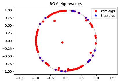
Figure 1: Linear Modal Model: True eigenvalues vs ROM’s computed eigenvalues for a 70 mode ROM. The true eigenvalues are the blue stars with the ROM eigenvalues the red circles. Overall, the computed ROM eigenvalues are close with the discrepancy due to both the ROM having half the modes as the true model and the additive noise. The evolution of (20) is in $\mathbb{C}^{n}$ rather than $\mathbb{R}^{n}$ due to the choice of complex $\lambda_{j}$’s; therefore, there will not be complex conjugate pairs.

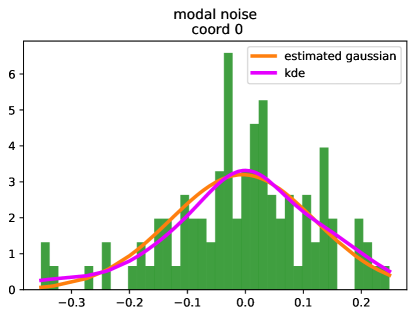
Figure 2: Linear Modal Model: Distribution of the modal noise $\rho(t)$ for the first coordinate of the 70 mode ROM. The actual distribution of the noise is given by the green histogram. The orange curve is the Gaussian distribution approximation derived from the modal noise sequence. The pink curve is a kernel density approximation of the distribution.

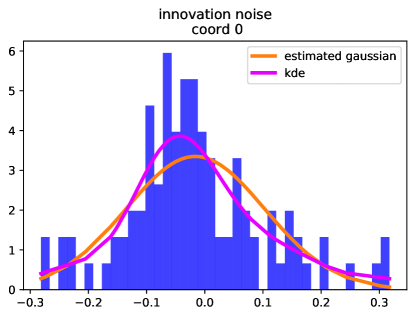
Figure 3: Linear Modal Model: Distribution of the innovation noise $\eta(t)$ for the first coordinate of the 70 mode ROM. The actual distribution of the noise is given by the blue histogram. The orange curve is the Gaussian distribution approximation derived from the modal noise sequence. The pink curve is a kernel density approximation of the distribution.

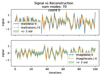
Figure 4: Linear Modal Model: Comparison of the reconstruction due to the ROM and the true signal for the first oscillator (indexed from 0). The true signal is given by the blue trace, the ROM reconstruction is the orange trace, and the green band is $\pm$2 standard deviations of the modal noise. The green band represent the 95% confidence interval for the ROM reconstruction. The top trace is the real part of the signal. The bottom trace is the imaginary part.

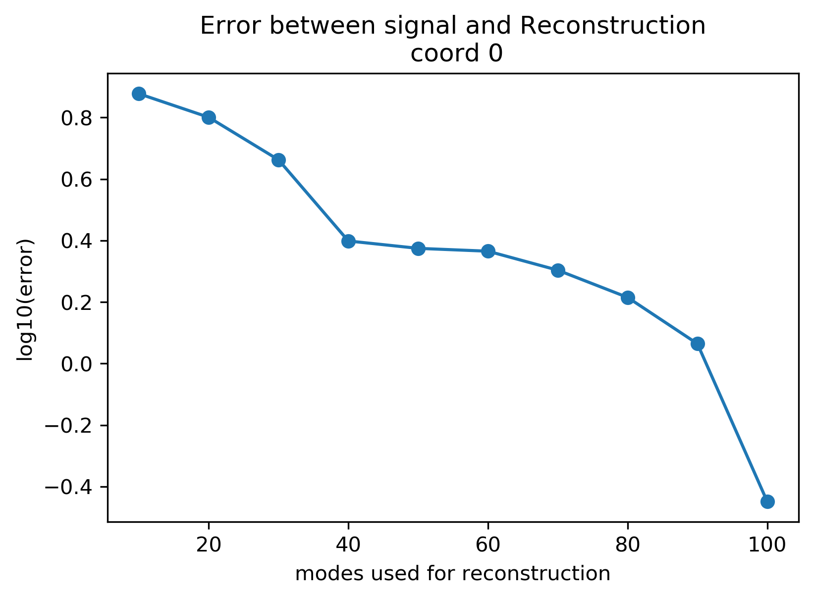
Figure 5: Linear Modal Model: Error vs number of reconstruction modes.

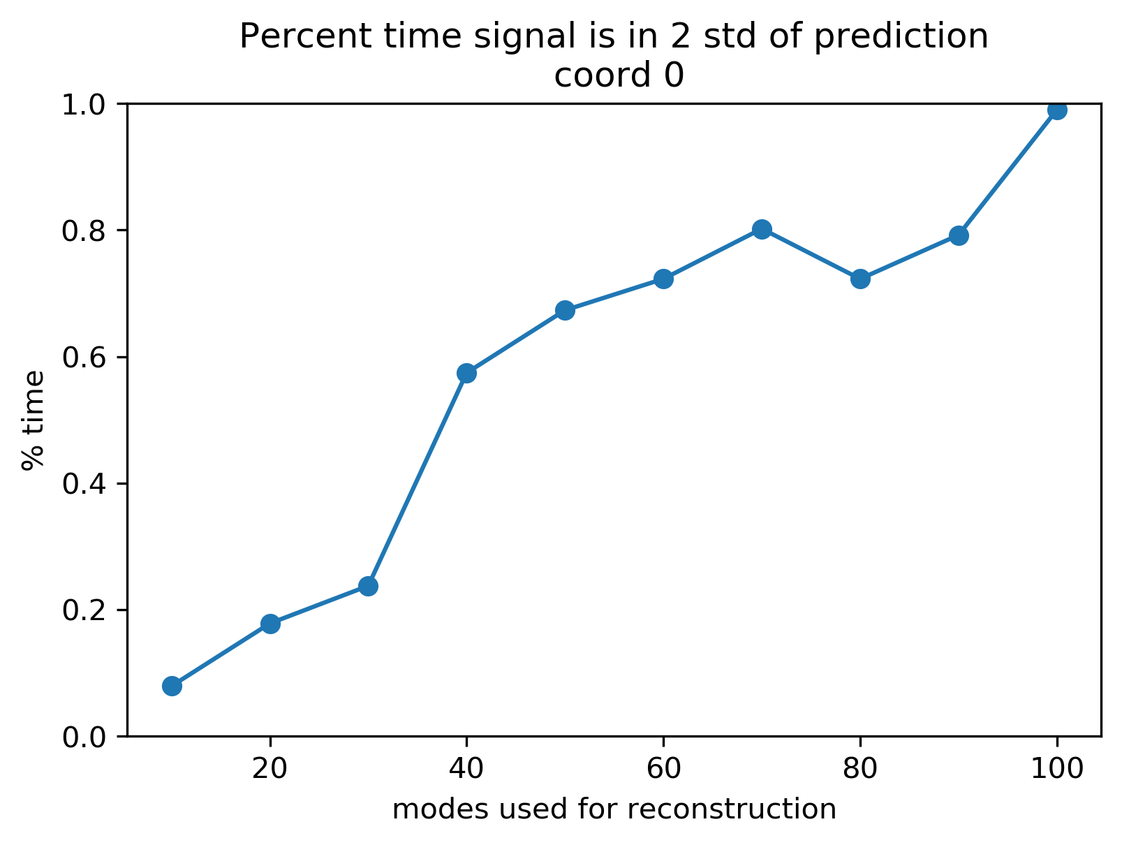
Figure 6: Linear Modal Model: Percent time true signal is within 95% confidence interval.

3.2 Switched Anharmonic Oscillators with additive noise

We apply the KROM methodology to a switched anharmonic oscillator example. A single anharmonic oscillator can be written in action-angle coordinates as

(21) $$\dot{I}(t)=0$$

(22) $$\dot{\theta}(t)=f(I(t))$$

where $I(t)$ is the action and $\theta(t)$ is the angle. Note that the rotational frequency $\dot{\theta}(t)$ depends on the action variable. For $f(I(t))=I(t)$, the higher the action, the faster the rotation. The anharmonic oscillator was chosen due to its lack of point spectra other than the eigenvalue at 1 corresponding to the constant eigenfunctions. It can be shown [16] that the rest of the spectrum is purely continuous with “eigenmeasures” $\phi_{j}(I,\theta)=e^{ij\theta}\delta(I-c)$ supported on level-sets $\{(c,\theta):\theta\in S^{1}\}$ of the action variable having eigenvalues $e^{ict}$.

For this example, we use a collection of anharmonic oscillators and randomly wire them together at each integer time point. At each integer time point, energy is instantaneously transferred from the oscillator with higher action to the one with lower action. Additionally, we incorporate an additive Gaussian noise term to the action variables. We investigate our prediction algorithm on such a system. Below, we give the construction of the model.

Let there be $j=0,\dots,n-1$ oscillators with action/angle dynamics given by

(23) $$I_{j}(t)-I_{j}(k) =\sum_{i}\mathbb{I}_{E(t)}((i,j))\,c_{j,i}(I_{i}(k)-I_{j}(k))+\eta_{j}(t),\qquad(k<t\leq k+1)$$

(24) $$\dot{\theta}_{j}(t) =f(I_{j}(t))$$

where $f(0)=0$ and $f$ is a nondecreasing function, $0<c_{j,i}<1$ and $c_{i,j}=c_{j,i}$, $E(t)$ is the set of undirected edges denoting the connections between oscillators at time $t$, and $\mathbb{I}_{E(t)}$ is the indicator function for the set $E(t)$, and $\eta_{j}(t)\sim N(0,\sigma^{2})$ is a normally distributed noise sequence . For example, $f(I)=I$ gives the anharmonic oscillator. Physically, the dynamics are as follows. We have a collection of nonlinear oscillators whose frequency increases as energy is injected into the oscillator. At any given time there are random connections between the oscillators, and energy flows from the oscillator of higher action (energy) to the one with lower action. Note that this is an instantaneous injection of energy at time $t=k+0^{+}$. With this formulation, the system is energy (action) conserving. In everything that follows, all edges are undirected edges.

3.2.1 Edge set dynamics.

Here, the edge set dynamics are given by permutation dynamics, although (23) allows for more random network connections. Let $\mathbf{y}(t),\mathbf{z}(t)\in\Theta(n)$ where $\Theta(n)$ is the set of all permutations of the vector $(0,\dots,n-1)$. Write $\mathbf{y}(t)=(y_{0}(t),\dots,y_{n-1}(t))$ (similarly for $\mathbf{z}(t)$). Let $\mathcal{P}(n)=\{\mathbf{P}:\Theta(n)\to\Theta(n)\}$ be the set of all permutation matrices on $\Theta(n)$. Fix $\mathbf{Y},\mathbf{Z}\in\mathcal{P}(n)$. Then

(25) $$\mathbf{y}(t) =\mathbf{Y}^{\lfloor t\rfloor}\mathbf{y}$$

(26) $$\mathbf{z}(t) =\mathbf{Z}^{\lfloor t\rfloor}\mathbf{z}$$

(27) $$E(t) =\{(y_{0}(t),z_{0}(t))\}$$

Here, the edge set changes at integer multiples in time and there is one random connection between oscillators (with it being possible an oscillator is connected to itself). The edge set consists of a single, undirected edge which connects oscillators $y_{0}(t)$ and $z_{0}(t)$ at time $t$. The state space of the full model is

(28) $$X=\{(\vec{I},\vec{\theta})\times(\mathbf{y},\mathbf{z}):I\in(\mathbb{R}^{+})^{n},\vec{\theta}\in(\mathbb{R}/\mathbb{Z})^{n},\mathbf{y},\mathbf{z}\in\Theta(n)\}.$$

and let the dynamics be given by Eqs. (23)–(27).

3.2.2 Experiments.

We show results for a range of the values so that the dynamics have a separation between scales between the speed of rotation of the oscillators and the time scale of switching the topology. Since the action variables $I$ directly control $\dot{\theta}$, then these variables can be changed to accomplish this separation of scale. The action variables $I$ will be distributed according to an exponential distribution. The $\lambda$ parameter for the exponential distributions (see eq. (29)) will be varied.

We will specify a distribution for the initial conditions. The exponential distribution is defined as

(29) $$h(t;\lambda)=\begin{cases}\lambda e^{-\lambda t},&t\geq 0\\ 0,&t<0.\end{cases}$$

The mean of this exponential distribution is $1/\lambda$. For $\vec{I}=(I_{1},\dots,I_{n})\in(\mathbb{R}^{+})^{n}$, we will take the $n$-product of exponential distributions

(30) $$H(\vec{I};\lambda)=\prod_{j=1}^{n}h(I_{j};\lambda)$$

The distribution for the initial conditions will be

(31) $$\mathbb{P}=H(\vec{I};1)\otimes dist(\vec{\theta})\otimes dist(\mathbf{y})\otimes dist(\mathbf{z}).$$

where $dist(\vec{\theta})$, $dist(\mathbf{y})$, and $dist(\mathbf{z})$ are the uniform distributions on their respective spaces. We draw initial conditions independently from the distribution:

(32) $$x^{(s)}=(\vec{I}^{(s)},\vec{\theta}^{(s)},\mathbf{y}^{(s)},\mathbf{z}^{(s)})\sim\mathbb{P},\qquad(s=1,\dots,S).$$

Fix the observable $\vec{f}\in L^{2}(X;\mathbb{C}^{n})$, which maps $X$ to $\mathbb{C}^{n}$, as

(33) $$\vec{f}(\vec{I},\vec{\theta},\mathbf{y},\mathbf{z})=(I_{1},\dots,I_{n},\theta_{1},\dots,\theta_{n})\in(\mathbb{R}^{+})^{n}\times(\mathbb{R}/\mathbb{Z})^{n}\subset\mathbb{R}^{2n}.$$

$\vec{f}$ does not directly observe the permutation variables $\mathbf{y},\mathbf{z}$. For this observable, compute a KMD for each sample of the initial conditions $x^{(s)}$. The following sections specify the lambda parameters used. When applying the DMD algorithm, we use a delay embedding of the observable $\vec{f}$ . For all simulations, we use a delay embedding of 300 time steps resulting in a data matrix of size $6,000\times 101$ for the DMD algorithm to act on. We therefore will be able to compute a maximum of 100 modes.

Table 1: Fixed parameters for KROM simulation

number of oscillators, $n$	10
numerical time step, $dt$	0.05 sec
simulation time, $t$	20 sec
$c_{i,j}$, for all $i,j$ (see eq. (23))	0.5
observable, $\vec{f}$	eq. (33)
Hankel delay embedding	300
$\lambda$	1
$\sigma$	0.05

Fig. 7 shows the eigenvalues of the reduced order models. The eigenvalues and Koopman modes were ordered by the norm of the Koopman mode from largest to smallest norm. To construct the models were take the $k$ top eigenvalues and Koopman modes to construct the $k$-th order model. Due to this, the eigenvalues of lower order models are always a subset of the eigenvalues of higher order models as can be seen in the figure.

Fig. 8 and Fig. 9 show the modal and innovation noise, respectively. For the 100 mode reconstruction (full reconstruction), the modal noise should be zero, since all the noise has been subsumed into the dynamics. The $10^{-14}$ is numerical error. The innovation noise is computed from projecting the dynamics on the orthogonal complement of $\mathbf{M}$, the modes used to construct the ROM. When $\mathbf{M}$ spans the entire space, then the projection onto the orthogonal complement is always 0, which is why the distribution of the innovation sequence for 100 modes is only supported on 0.

In Fig. 10, it is notable that the signal reconstruction gets better when around 50 modes are used (in fact, that number is somewhat lower (see Fig. 21). The heuristic dictates that 40 modes is the minimum number of modes that can be used for the model, as this is where the modal noise becomes approximately Gaussian.

Fig. 12 shows the error of the ROM’s prediction vs. the number of modes used in the model. The error of the reconstruction does not, however, reflect the accuracy of the ROM prediction. Namely, the ROM has been computed from a noisy signal, and thus the representation with a full number of modes subsumes noise into coherent modal dynamics.

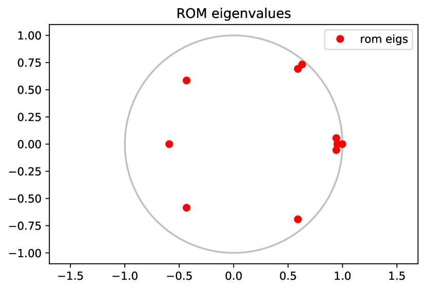
(a) 10 modes

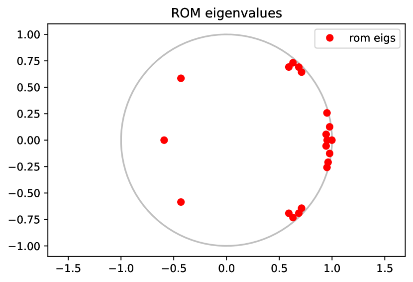
(b) 20 modes

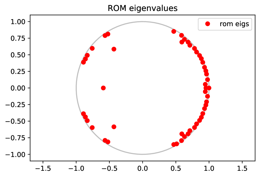
(c) 50 modes

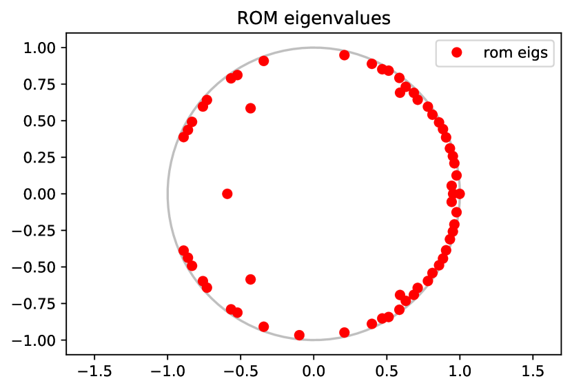
(d) 60 modes

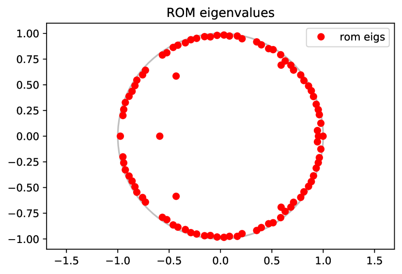
(e) 90 modes

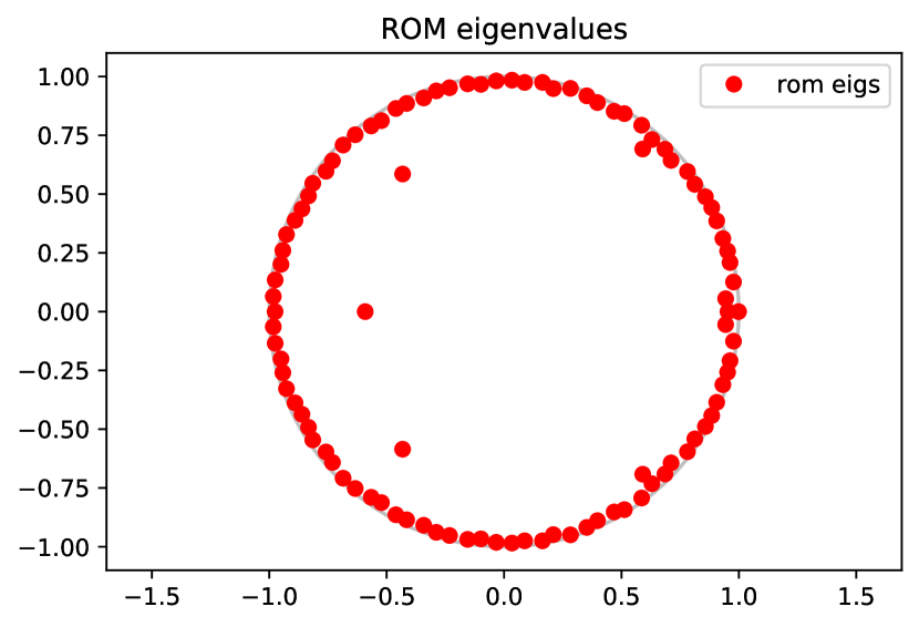
(f) 100 modes

Figure 7: Anharmonic Oscillators. Computed Koopman eigenvalues for the switched anharmonic oscillator model with added added Gaussian noise $(\sim N(0,0.05^{2})$.

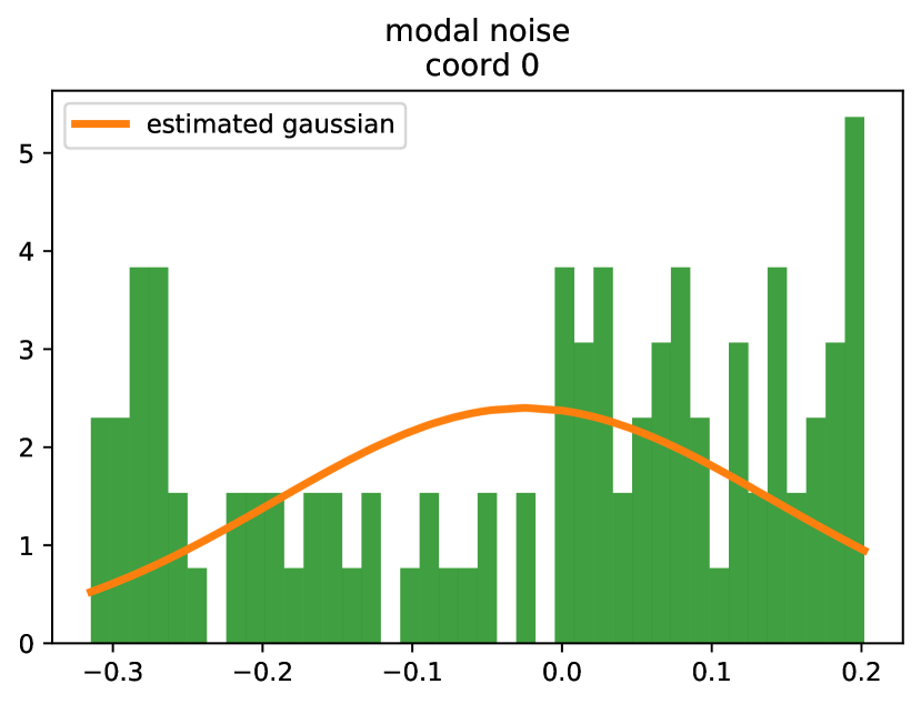
(a) 10 modes

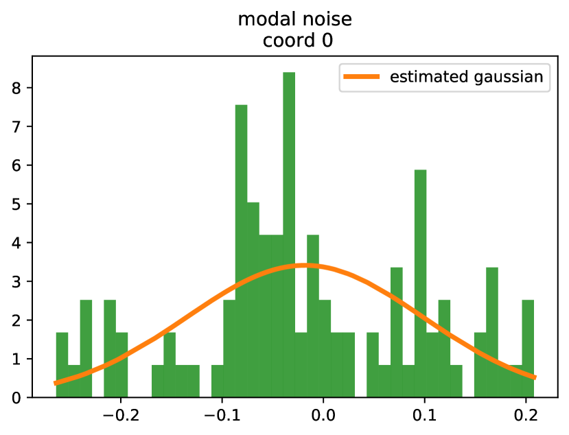
(b) 20 modes

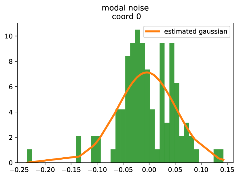
(c) 50 modes

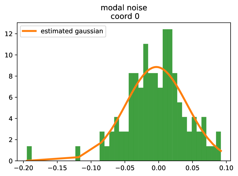
(d) 60 modes

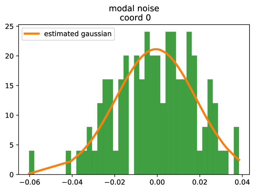
(e) 90 modes

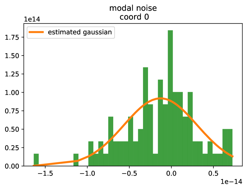
(f) 100 modes

Figure 8: Anharmonic Oscillators. The in-plane modal noise for oscillator 0. We estimate the Gaussian by computing the standard deviation of the modal noise distribution. The estimated standard deviation will be used to compute the confidence bounds for the reduced order models signal. Note the decreasing range of the scales on the x-axis as the number of modes increases. These results are typical for the other oscillators as well.

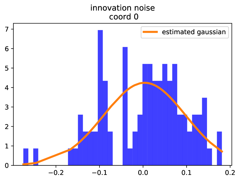
(a) 10 modes

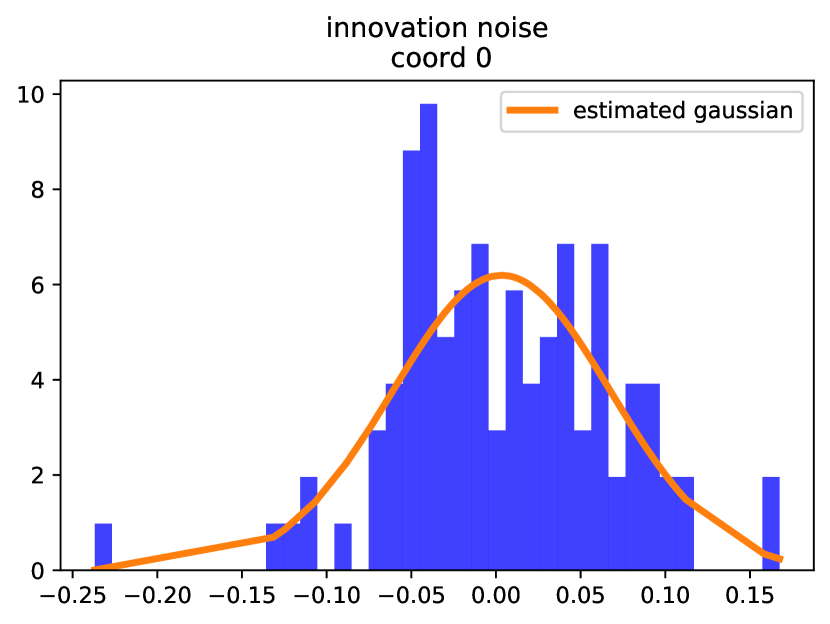
(b) 20 modes

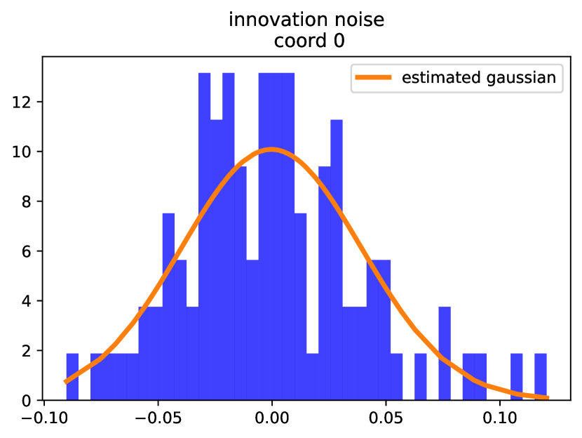
(c) 50 modes

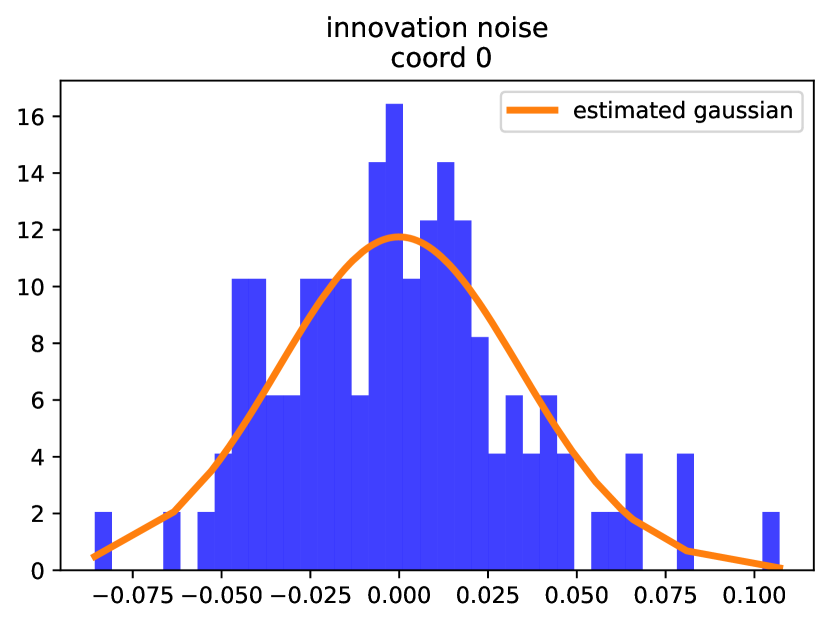
(d) 60 modes

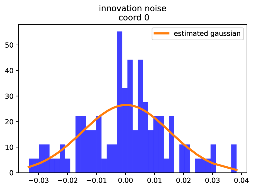
(e) 90 modes

(f) 100 modes

Figure 9: Anharmonic Oscillators. The out-of-plane innovation noise for the for oscillator 0. These results are typical for the other oscillators as well.

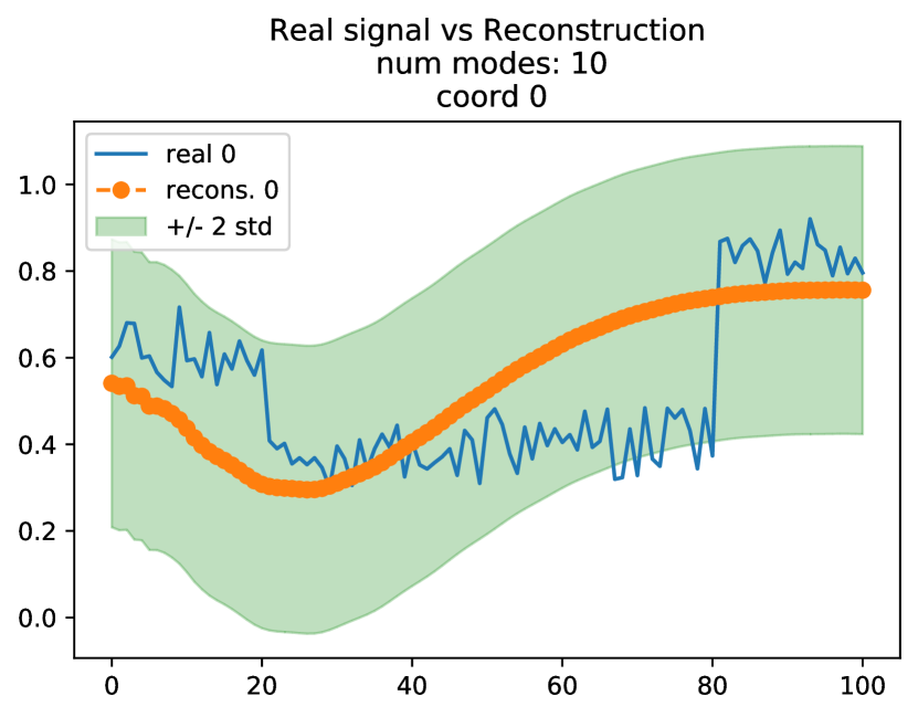
(a) 10 modes

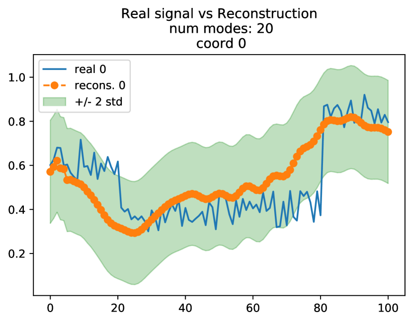
(b) 20 modes

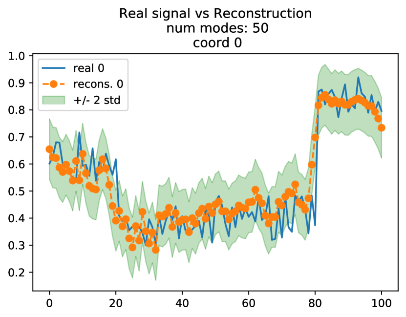
(c) 50 modes

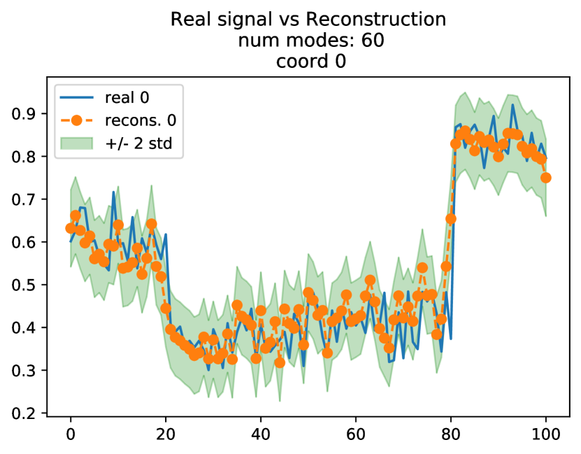
(d) 60 modes

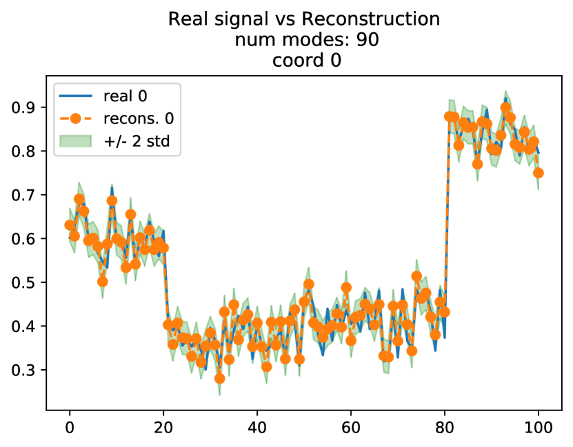
(e) 90 modes

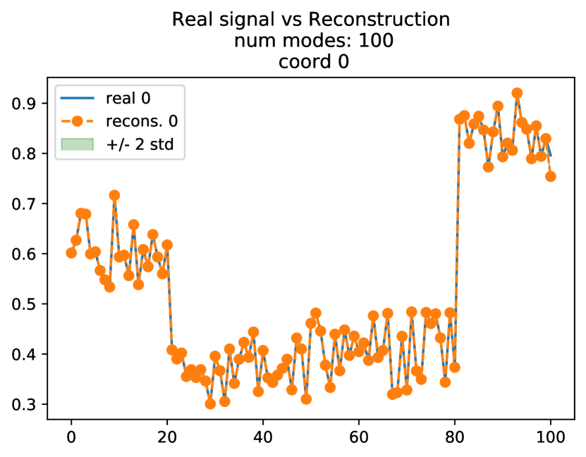
(f) 100 modes

Figure 10: Anharmonic Oscillators Action. Comparison between the reduced order model (ROM) signal (orange) with the real signal (blue) for the action variable of oscillator 0. The 95% confidence interval is given by the green band around the orange signal. As the number of reconstruction modes increases, the ROM signal follows the true signal better and the 95% confidence becomes tighter. These results are typical for the other oscillators as well

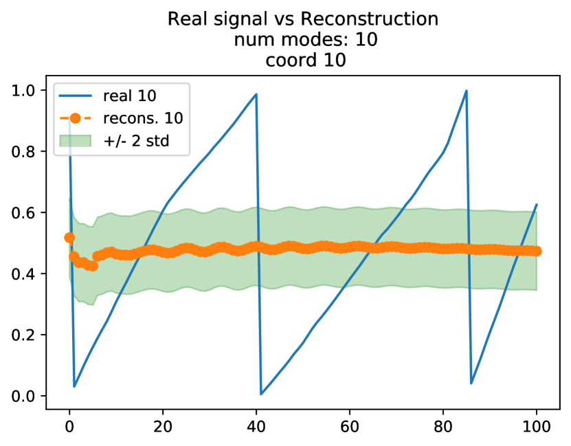
(a) 10 modes

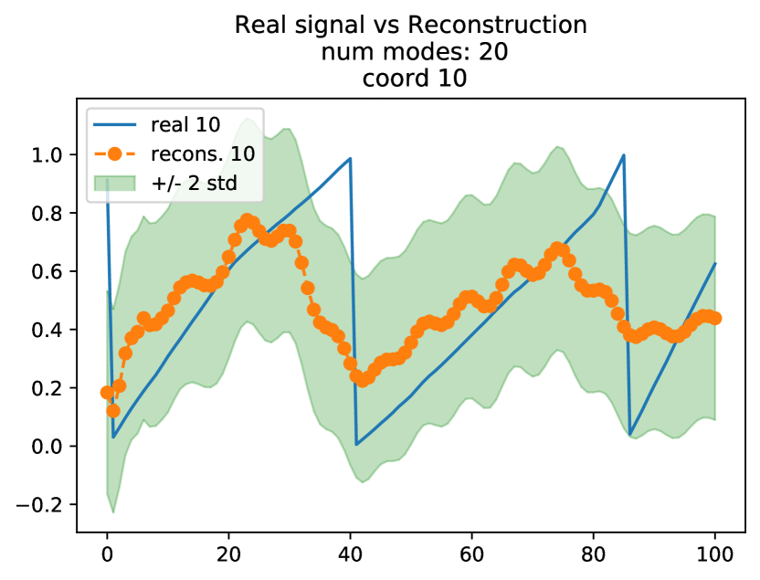
(b) 20 modes

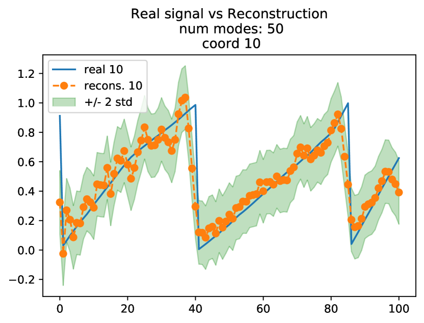
(c) 50 modes

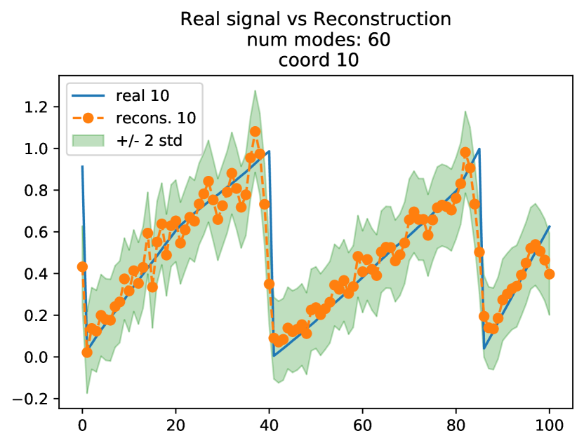
(d) 60 modes

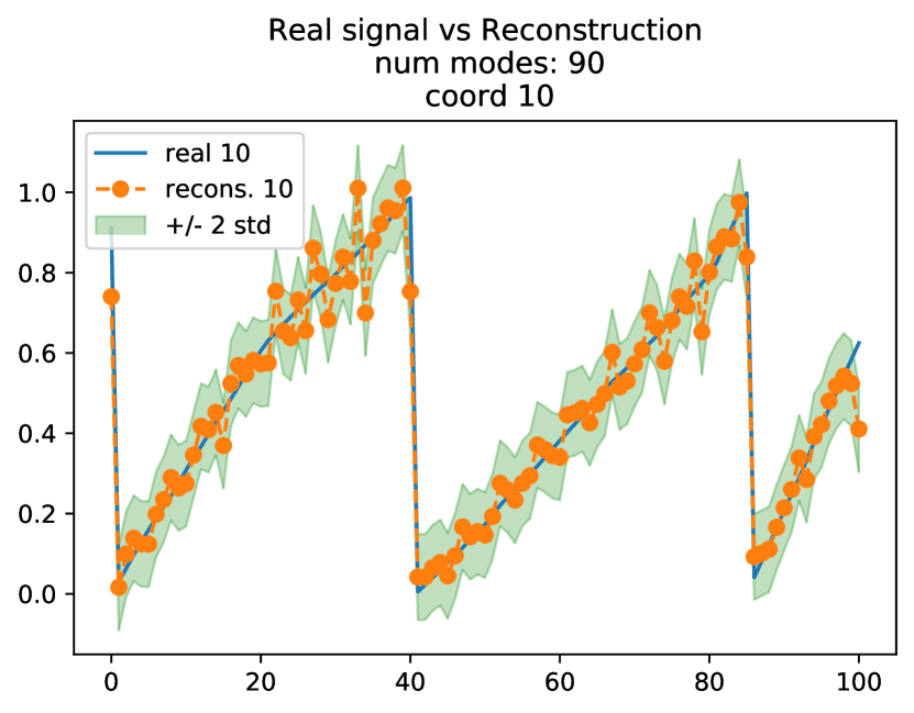
(e) 90 modes

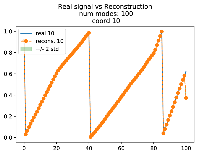
(f) 100 modes

Figure 11: Anharmonic Oscillators Angles. Comparison between the reduced order model (ROM) signal (orange) with the real signal (blue) for the angle variable of oscillator 0. The 95% confidence interval is given by the green band around the orange signal. As the number of reconstruction modes increases, the ROM signal follows the true signal better and the 95% confidence becomes tighter. These results are typical for the other oscillators as well

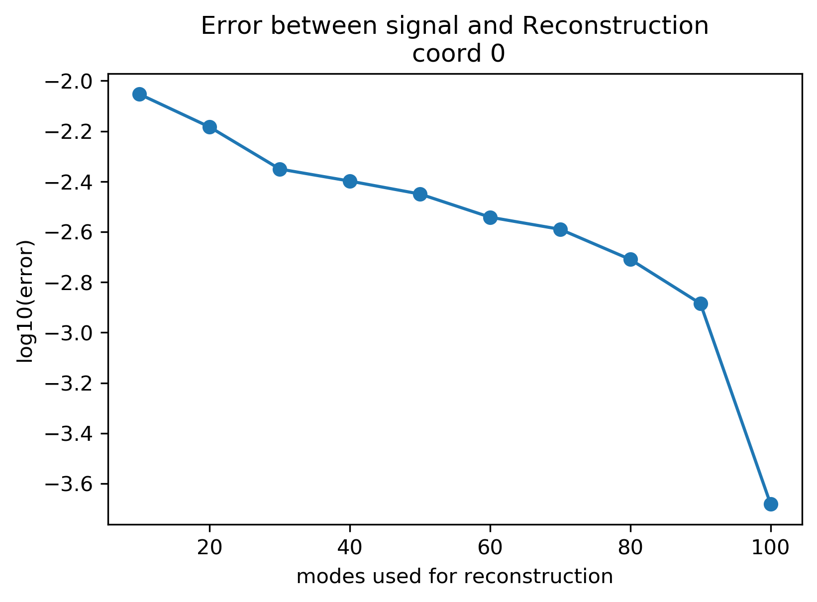
(a) Oscillator 0 action variable.

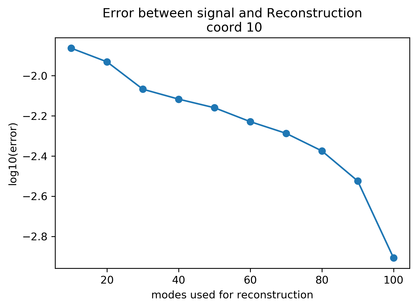
(b) Oscillator 0 angle variable.

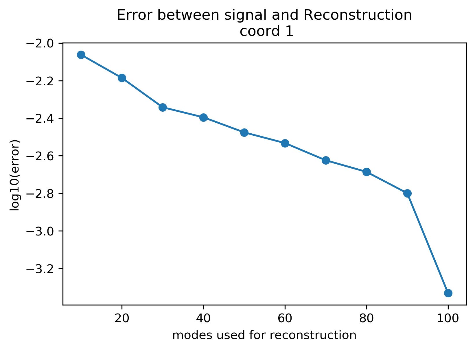
(c) Oscillator 1 action variable.

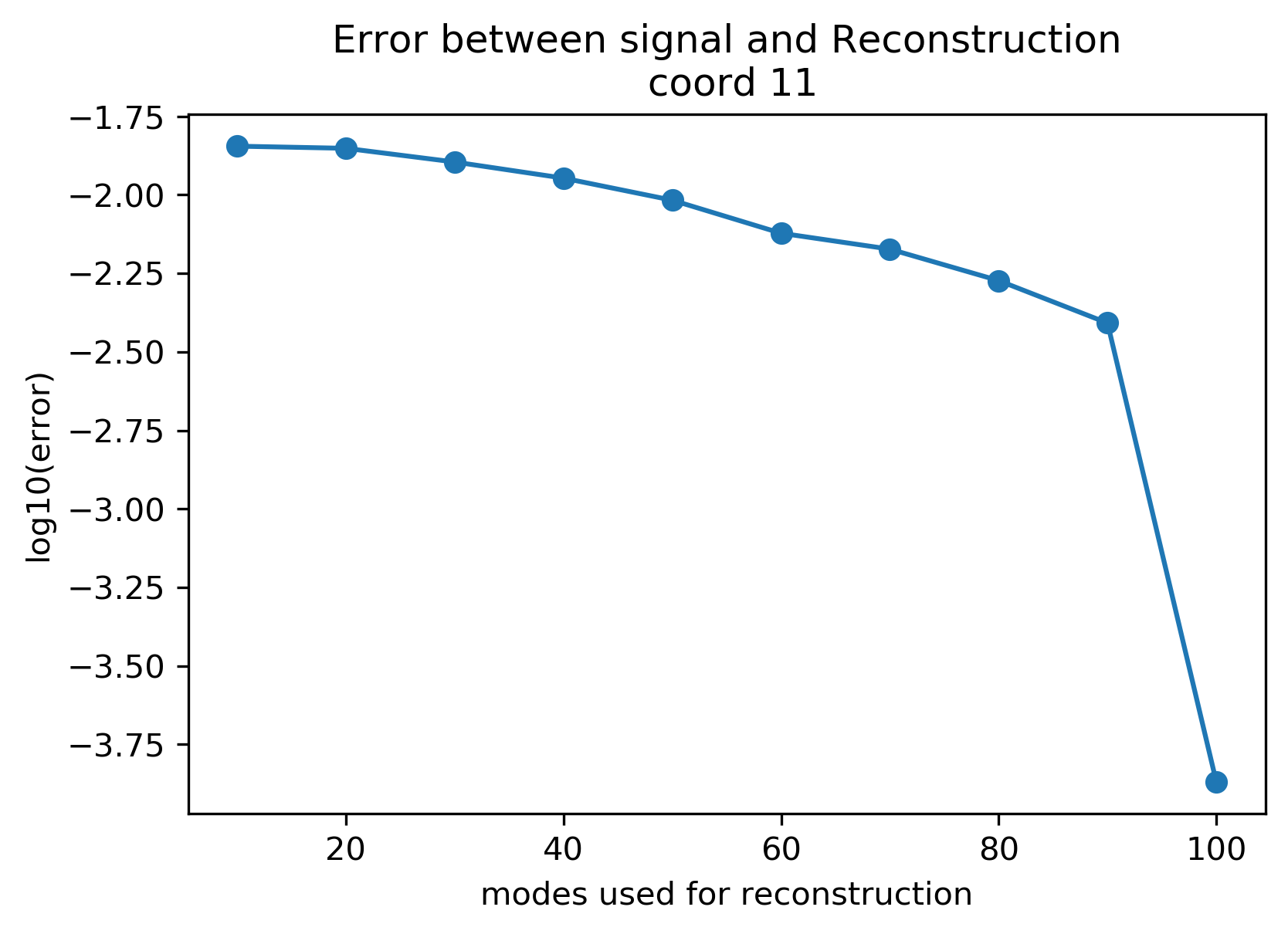
(d) Oscillator 1 angle variable.

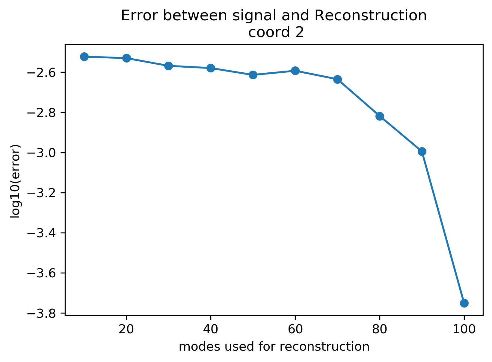
(e) Oscillator 2 action variable.

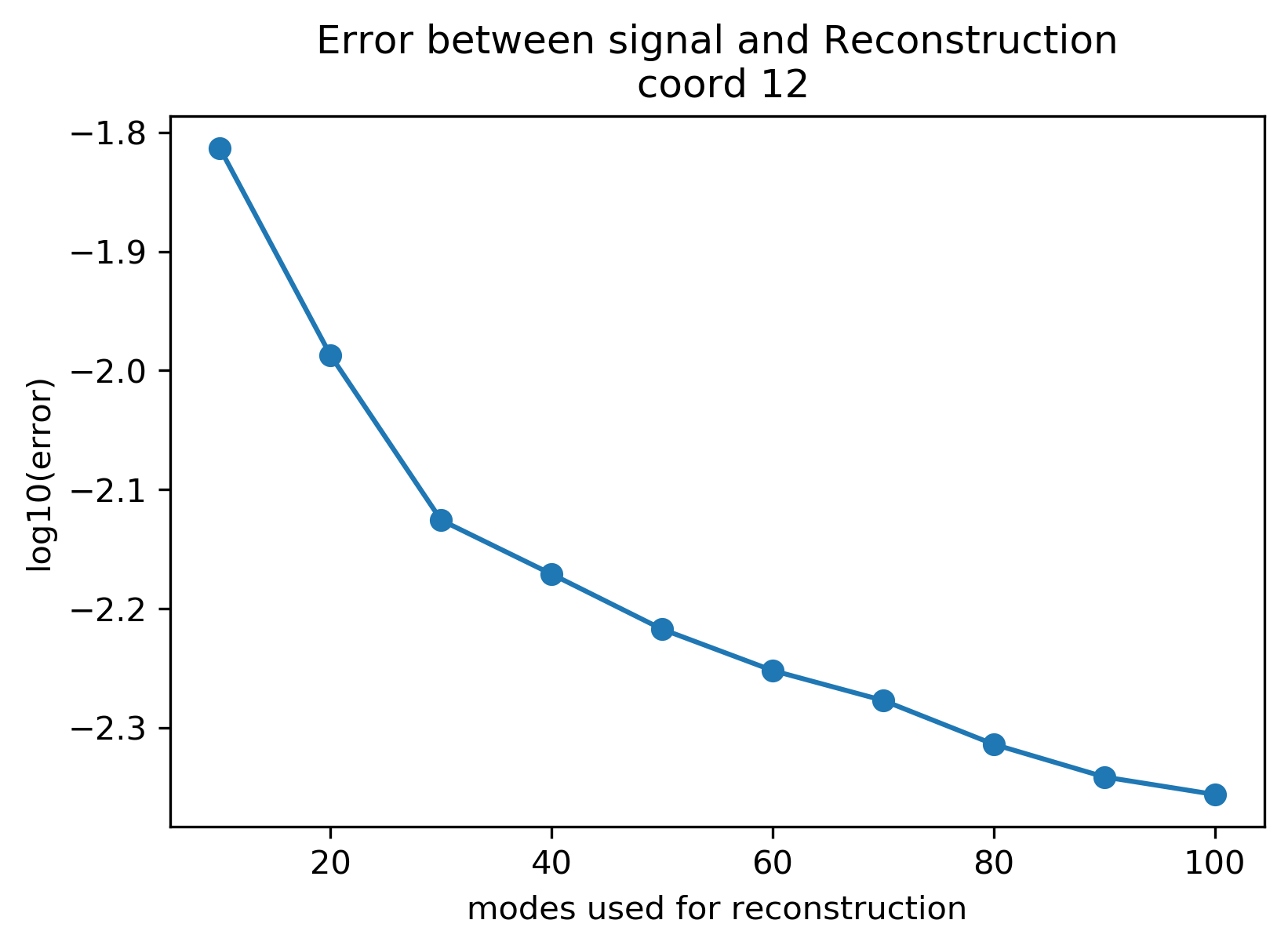
(f) Oscillator 2 action variable.

Figure 12: Anharmonic Oscillators. Reconstruction errors of action and angle variables vs. number of modes used for the reconstruction for 3 of the oscillators.

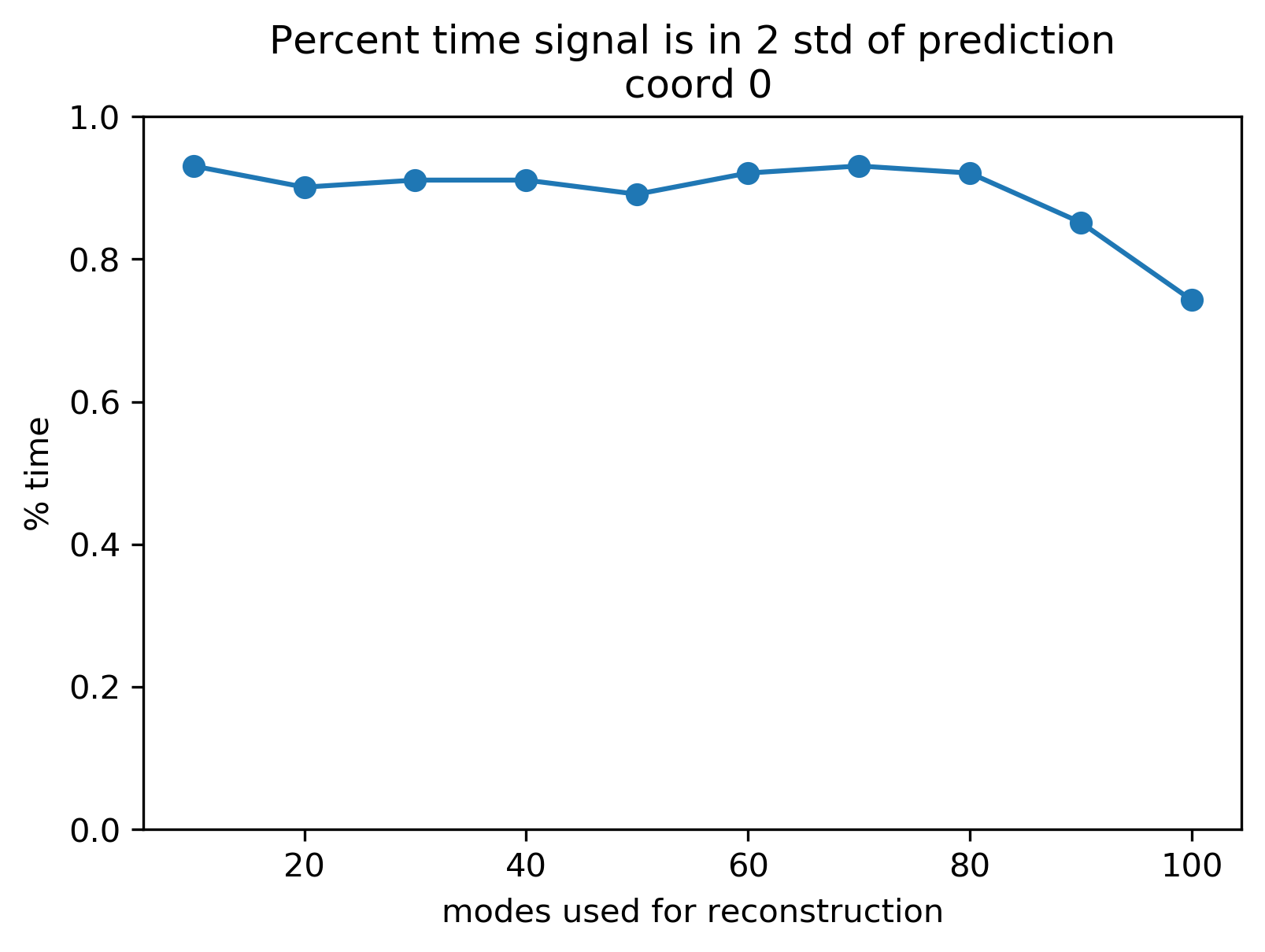
(a) Oscillator 0 action variable.

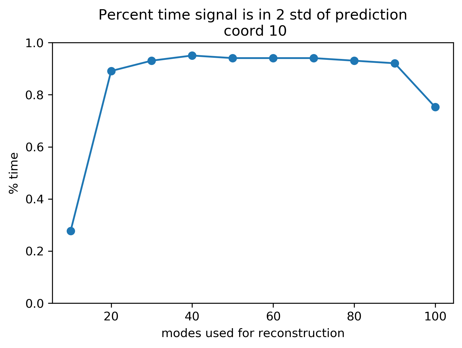
(b) Oscillator 0 angle variable.

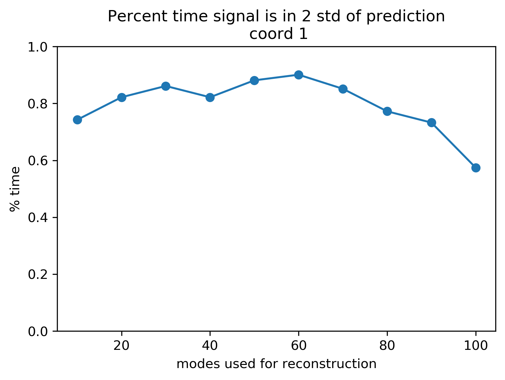
(c) Oscillator 1 action variable.

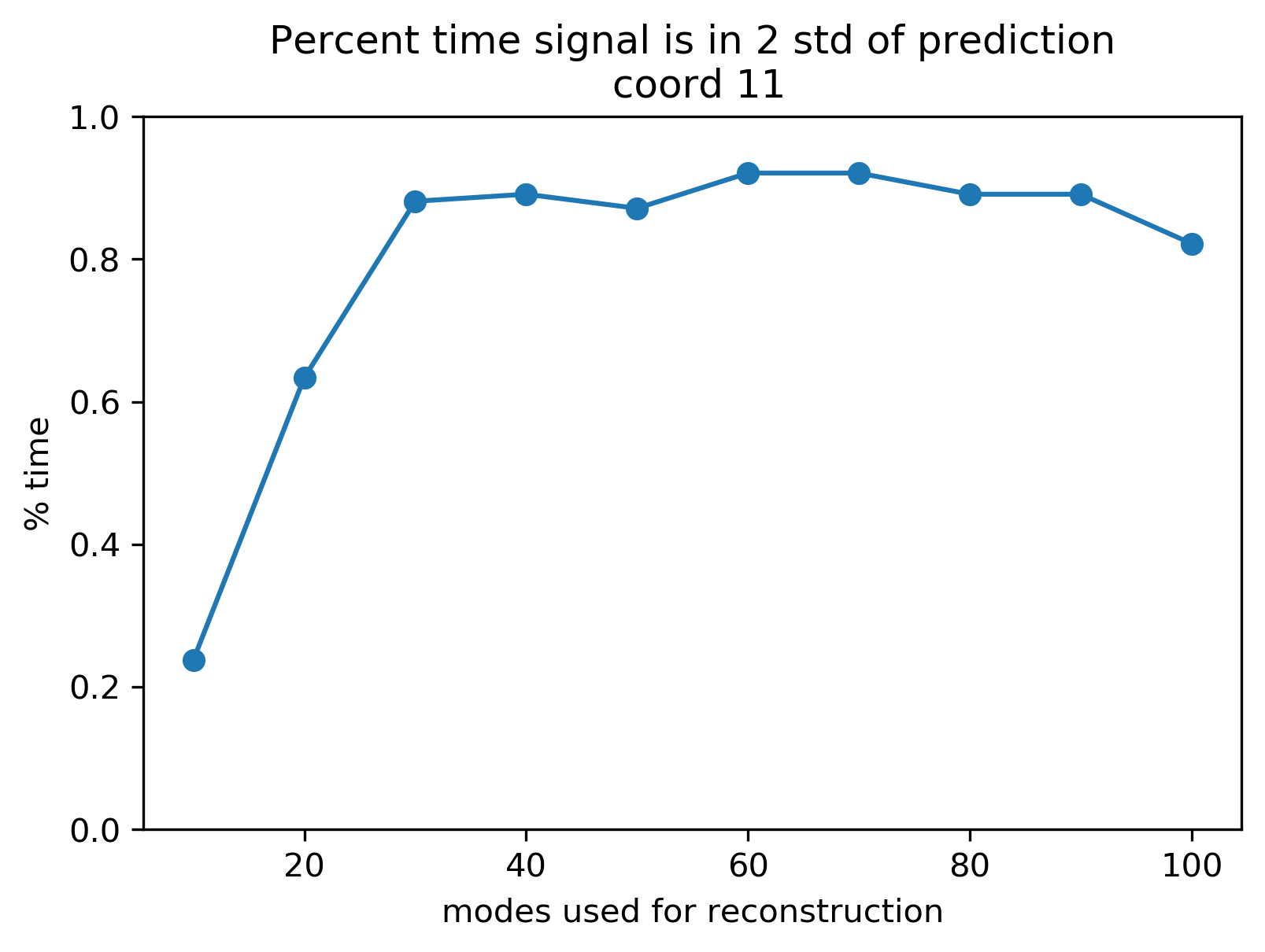
(d) Oscillator 1 angle variable.

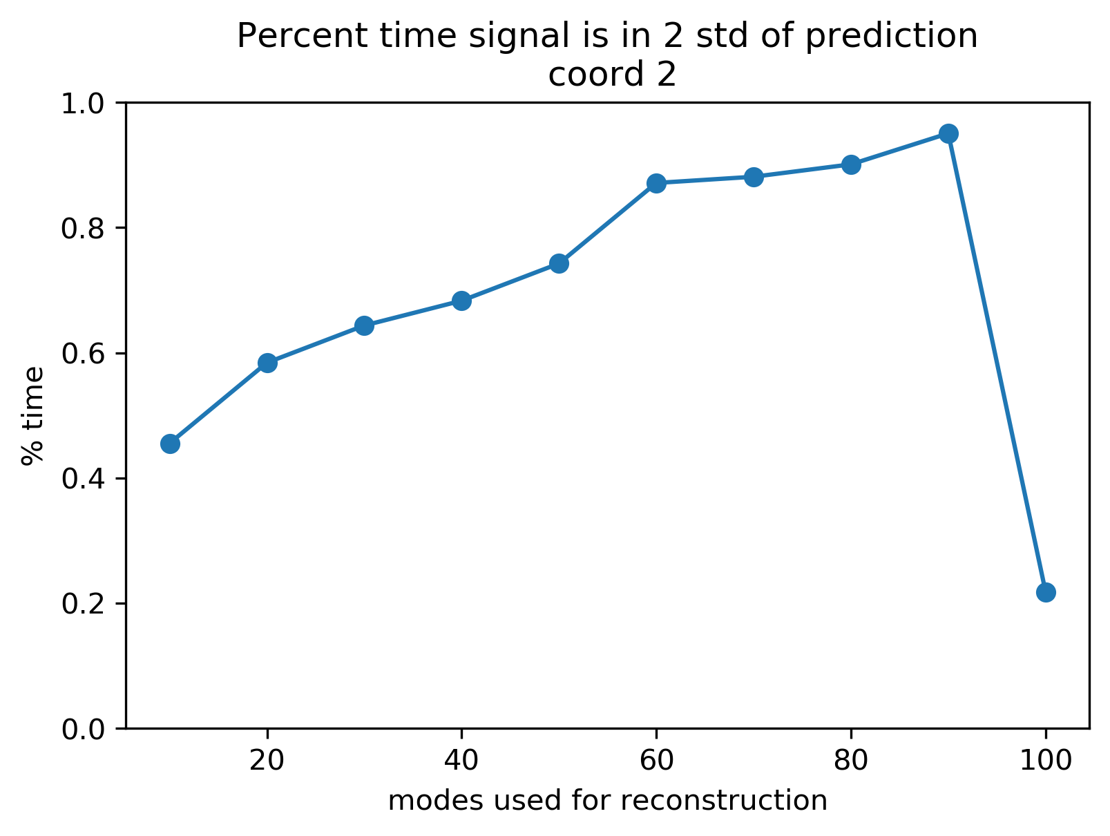
(e) Oscillator 2 action variable.

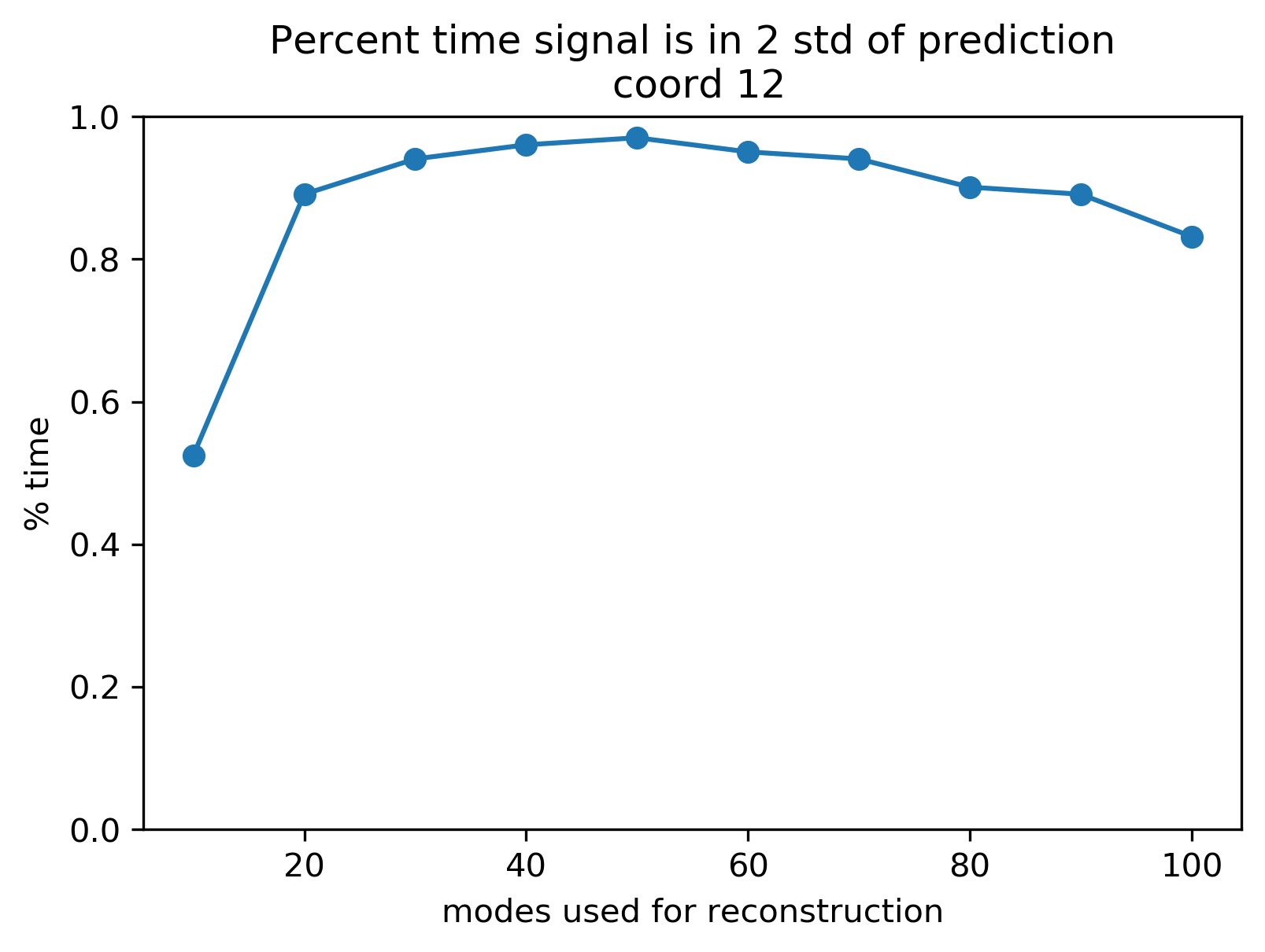
(f) Oscillator 2 action variable.

Figure 13: Anharmonic Oscillators. Percent of time that the true signal is within the 95% confidence interval. The large drop in the residence times when using 100 modes is due to the relative error between the signal and the standard deviation of the modal noise. When using a large number of modes for the ROM, the noise gets subsumed into the deterministic model. When using the full number of modes (100), we see in Fig. 8 that the computed modal noise’s standard deviation is on the order of $10^{-14}$, meaning that the noise has been fully subsumed into the deterministic dynamics. The error between the ROM and the signal is on the order of $10^{-2}$ to $10^{-4}$ and thus adding a $10^{-14}$ confidence bound rarely contains the true signal.

3.3 Kuramoto Model

As our final example for applying the KROM, we turn to the Kuramoto model of coupled oscillators [1]. In the classical model (see eq.Eq. 34), the strength of the connections between the oscillators is fixed and uniform for all oscillators. As the strength of the connection increases, the oscillators can display behaviors such as synchronization [1].

(34) $$\frac{d\theta_{i}}{dt}=\omega_{i}+\xi_{i}+\frac{K}{N}\sum_{j=1}^{N}\sin(\theta_{j}-\theta_{i}).$$

Here, we introduce a modification where instead of the fixed coupling strength $K/N$ we introduce randomness. Our enhanced model looks like

(35) $$\frac{d\theta_{i}}{dt}=\omega_{i}+\xi_{i}+\sum_{j=1}^{N}\frac{K+\zeta_{i,j}}{N}\sin(\theta_{j}-\theta_{i}).$$

In our examples, each $\zeta_{i,j}$ is distributed according to $N(0,\sigma^{2})$, with $\sigma=1$, $K=5$, and $N=10$. The $N\times N$ coupling matrix $Z=[\zeta_{i,j}]_{1\leq i,j\leq N}$ is restricted to be symmetric with $\zeta_{i,j}=\zeta_{j,i}$. In our experiments, we have chosen to set $\xi_{i}\sim N(0,0.25)$ for all $i$. The natural frequencies were drawn uniformly at random from the interval $[0.25,0.75]$, whereas the initial condition for each coordinate of $\theta$ was chosen uniformly at random from the interval $[0,2\pi]$. When constructing the data matrix we use a complex representation of the angles ($\theta\mapsto z=\exp(i\theta)$).

Table 2: Fixed parameters for Kuramoto model simulation

number of oscillators, $N$	10
numerical time step, $dt$	0.05 sec
simulation time, $t$	20 sec
Nominal coupling strength, $K$	5
Effective coupling strength, $K/N$	0.5
Randomly coupling strength, $\zeta_{i,j}=\zeta_{j,i}$	$\sim N(0,1)$
Effective Randomly coupling strength, $\zeta_{i,j}/N=\zeta_{j,i}/N$	$\sim N(0,1)/10$
Additive Gaussian noise, $\xi_{i}$	$\sim N(0,0.25)$
observable, $\vec{f}$	$z=\exp(i\theta)$
Hankel delay embedding	300
Natural frequencies, $\omega_{i}$	$\sim U([0.25,0.75])$
Initial conditions, $\theta_{i}(0)$	$\sim U([0,2\pi])$

Fig. 14 shows the reduced order models’ eigenvalues for models with 20, 50, 70, and 100 modes used for reconstruction. The set of eigenvalues form a strictly nested sequence of sets parameterized by the number of modes used for reconstruction. Specifically, the set of eigenvalues of the 20 mode model is a strict subset of the set of eigenvalues for the 50 mode model which is a strict subset of 70 mode model’s eigenvalues, etc. This is a general property of the Koopman ROM algorithm since the method uses the data to compute all of the modes, orders them according to their norm, and then selects a subset in order to build a reduced order model. Another property to note is the distribution of the eigenvalues in the complex plane. The Type 2 models are distributed in a wedge $W=\{re^{is}:\forall r\in[0,1],\forall s\in(-\phi,\phi),\phi\in[0,\pi]\}$ with $\phi$ increasing with increasing number of modes used for reconstruction.

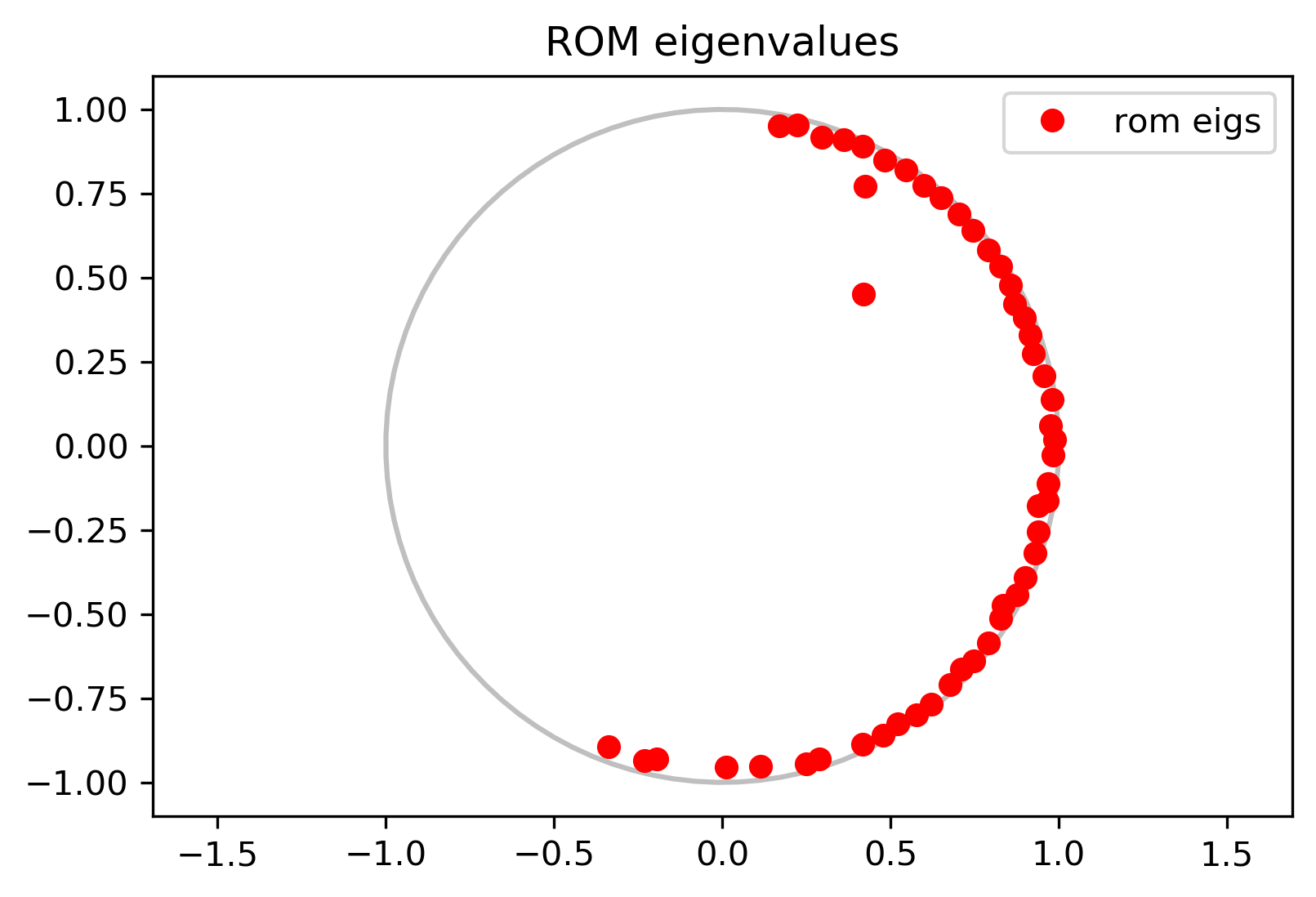
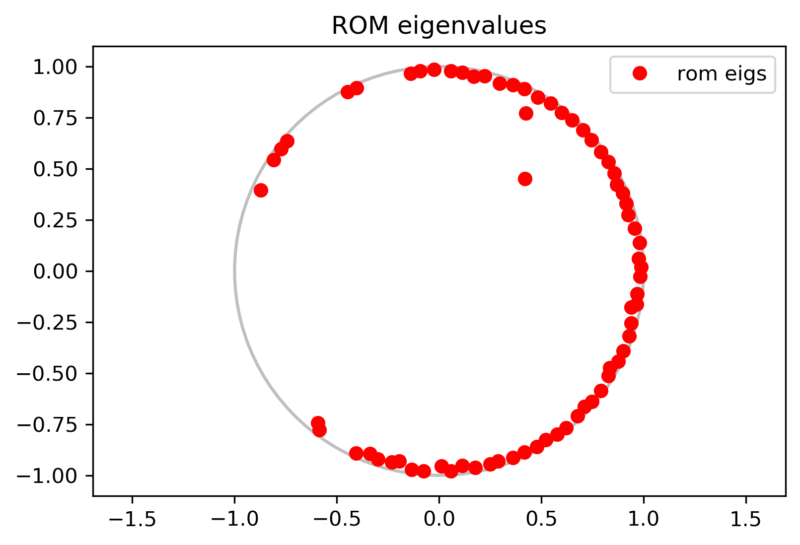
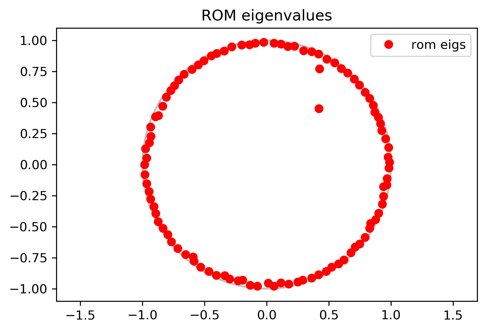
Figure 14: Kuramoto models, ROM eigenvalues: Top left: ROM with 20 modes. Top right: ROM with 50 modes. Bottom left: ROM with 70 modes. Bottom right: ROM with 100 modes (full reconstruction). We note that we use the complexification of the real angles, $\theta\mapsto\exp(i2\pi\theta)$, in the construction of the data matrix. Since the data matrix is complex rather than real, complex-conjugate pairs of eigenvalues are not enforced, resulting in an asymmetric spectrum.

Fig. 15 shows the reconstruction of the signal of the first oscillator. The ROMs predictions converge rapidly to the true signal as the number of modes increases. Additionally, the computed variance rapidly converges to 0. In fact, one cannot distinguish a $\pm 2$ standard deviation band when using 60 modes or greater. See the appendix Appendix A for a comparison of these reconstructions when using real angles $\theta\in[0,2\pi)$ and when using the complexified angles $z=\exp(i\theta)$. That discussion shows that since the KMD algorithms minimize loss functions using Euclidean distances, a representation for a variable needs to be determined where the Euclidean distance in that new representation closely approximates the natural norm for the original representation of the variable.

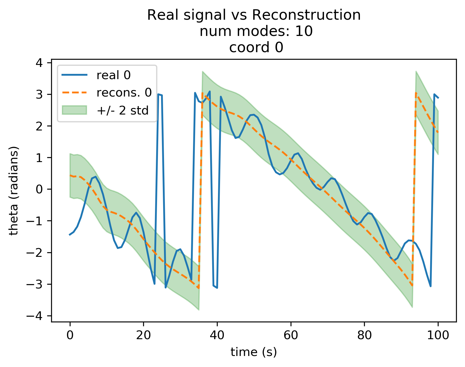
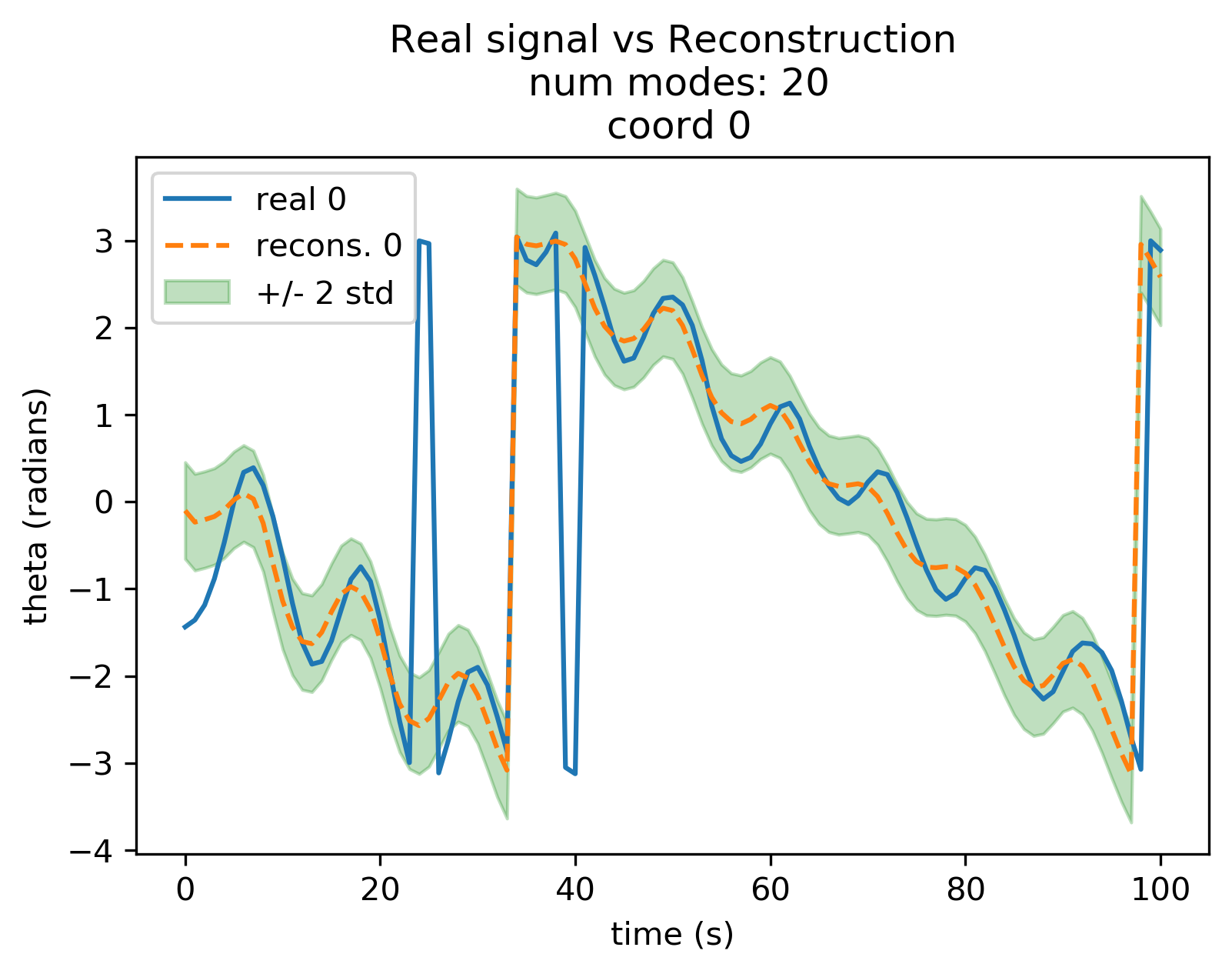
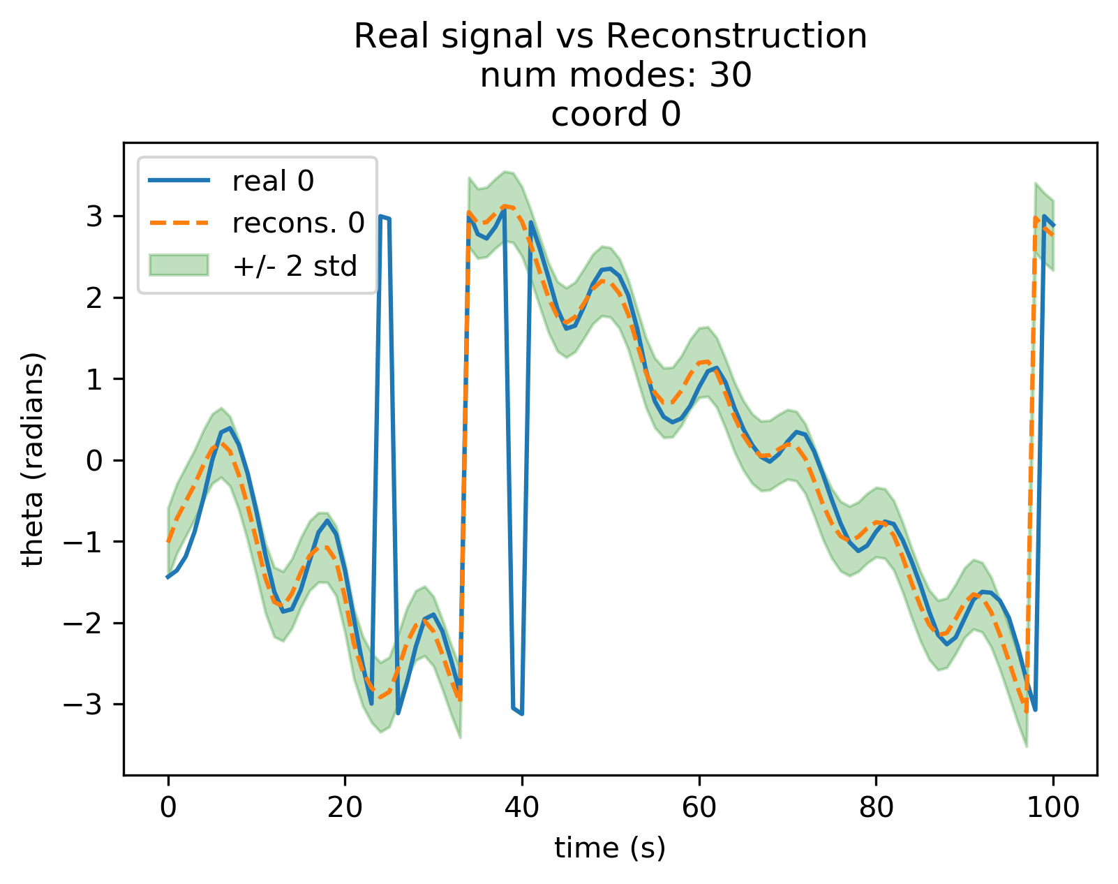
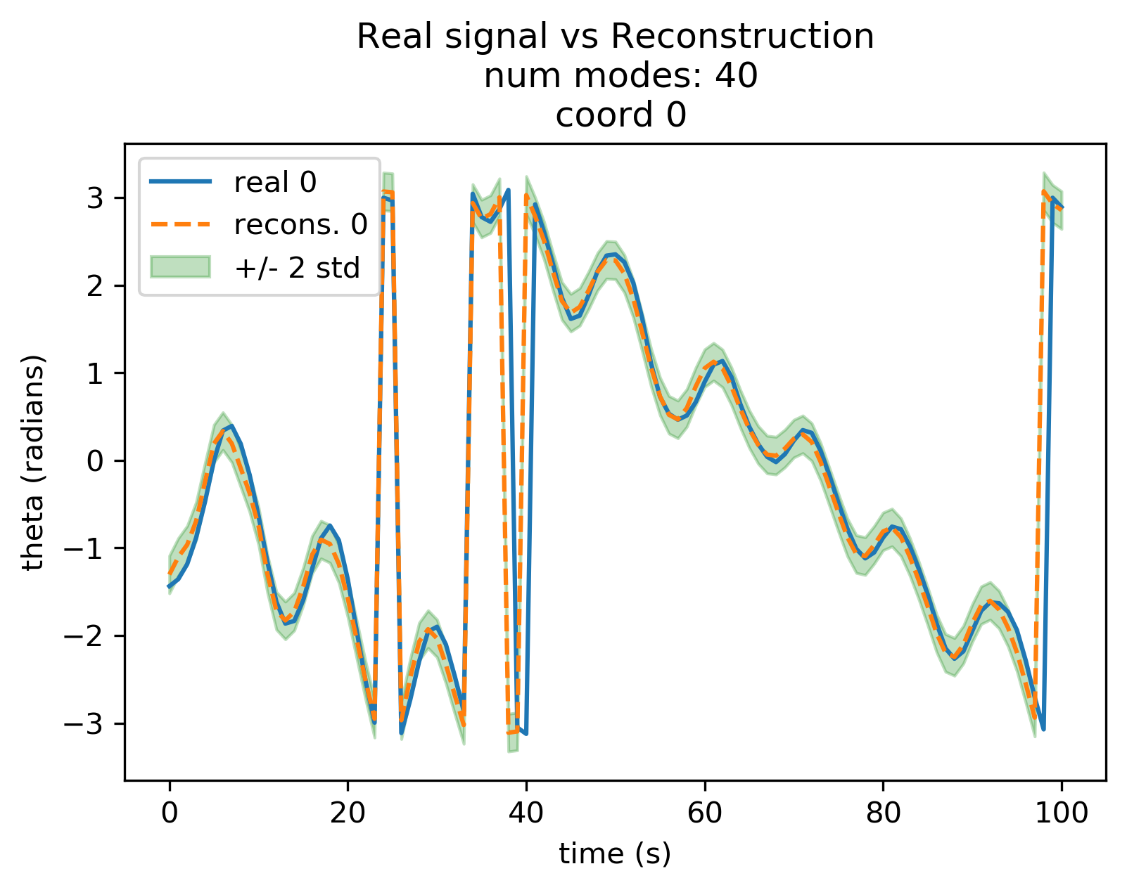
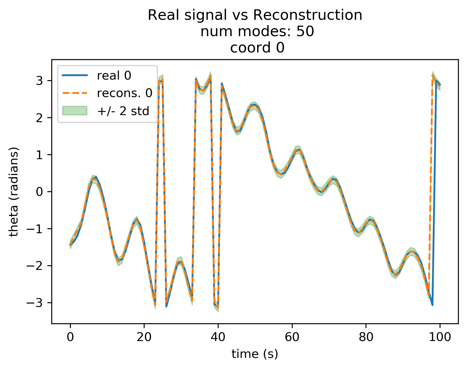
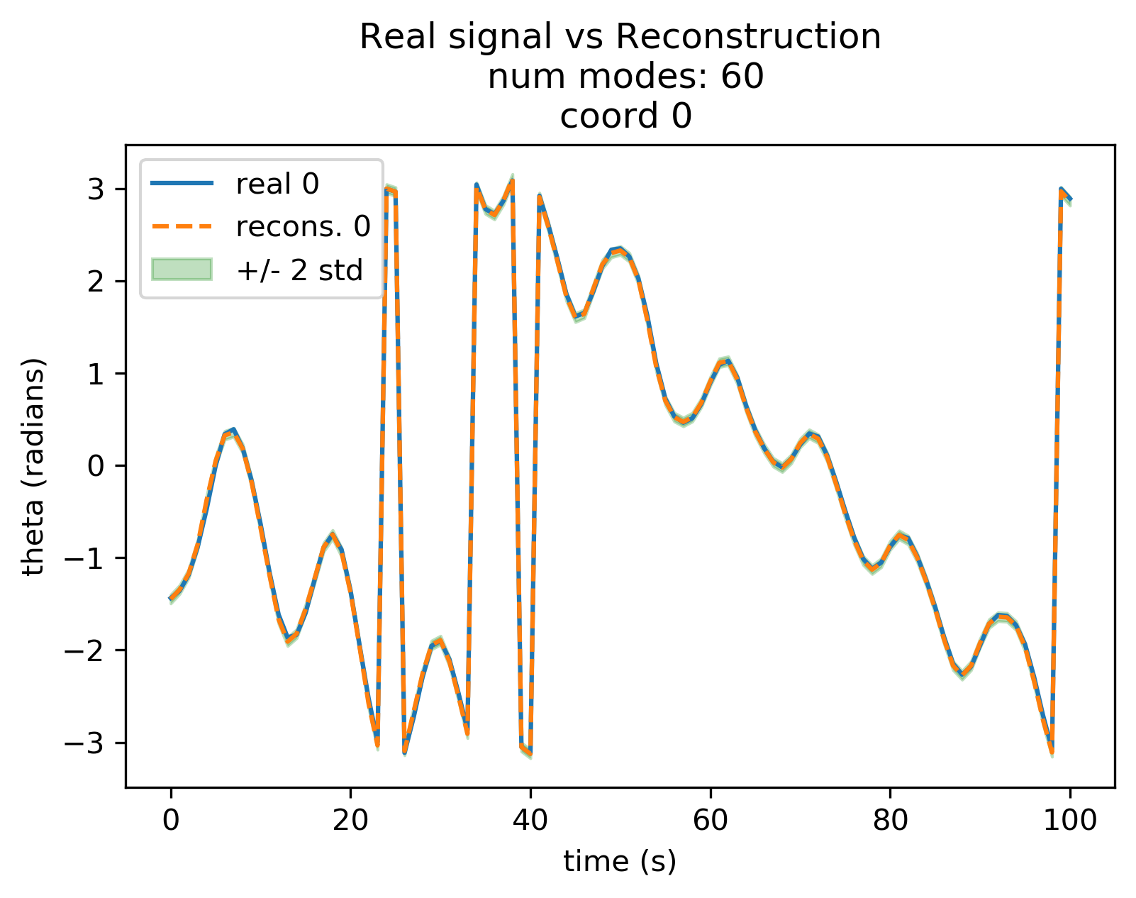
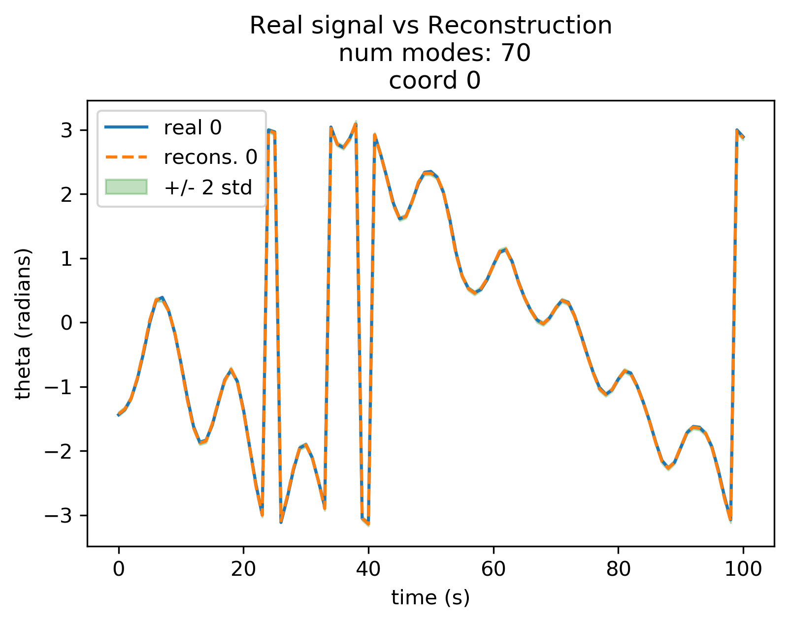
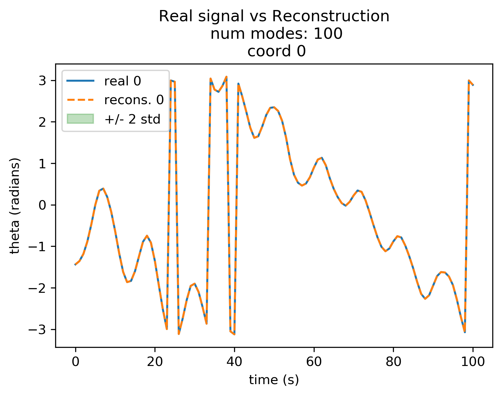
Figure 15: Kuramoto models, signal vs reconstruction: Comparison of the true signal with reconstruction signals using $10,20,30,\dots,100$ modes for reconstruction for oscillator 0. The true signal is in blue. The reconstruction signal is orange and the green band is $\pm 2$ standard deviations of the modal noise.

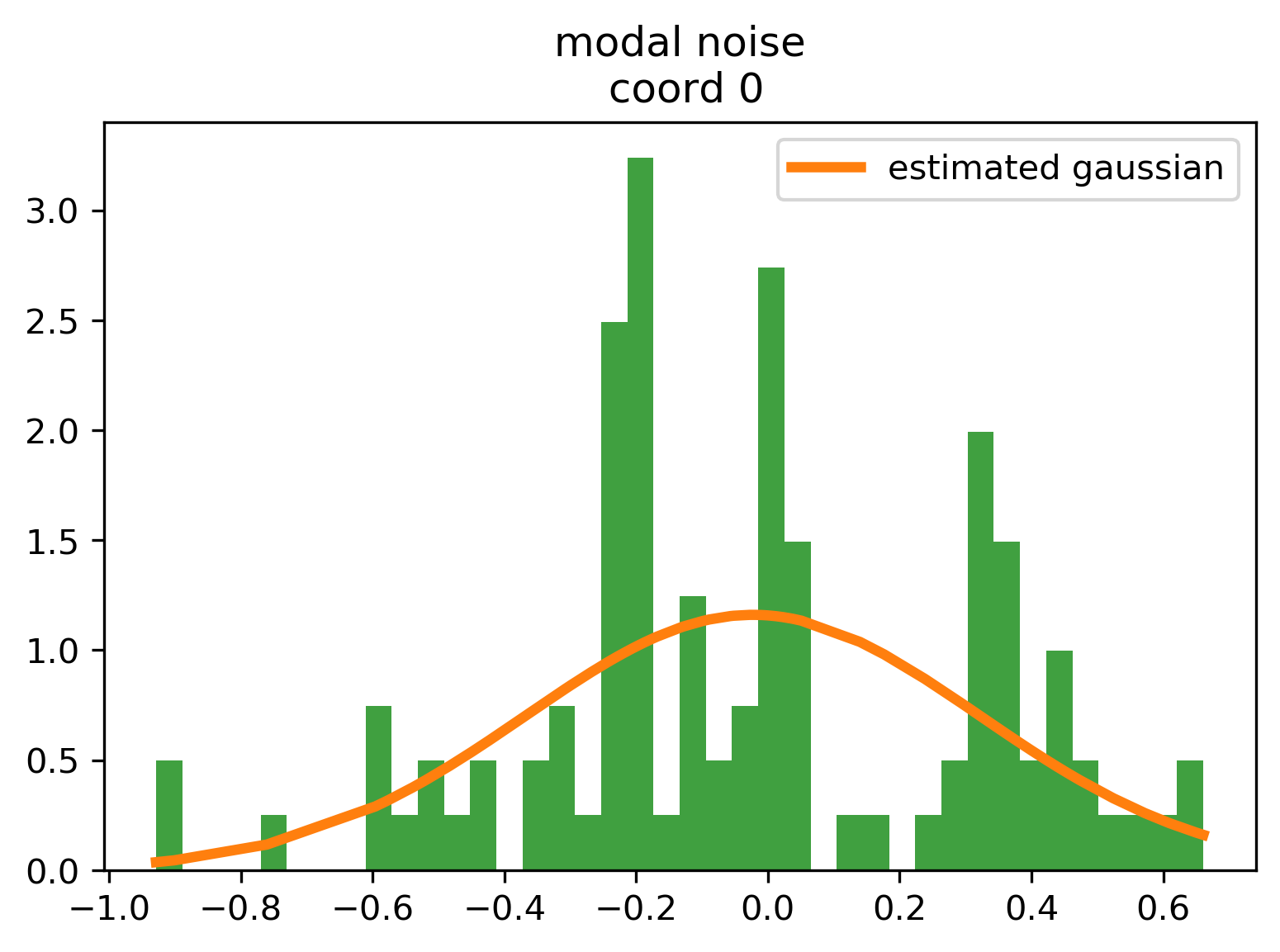
(a) 10 modes

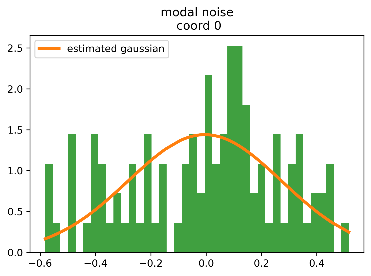
(b) 20 modes

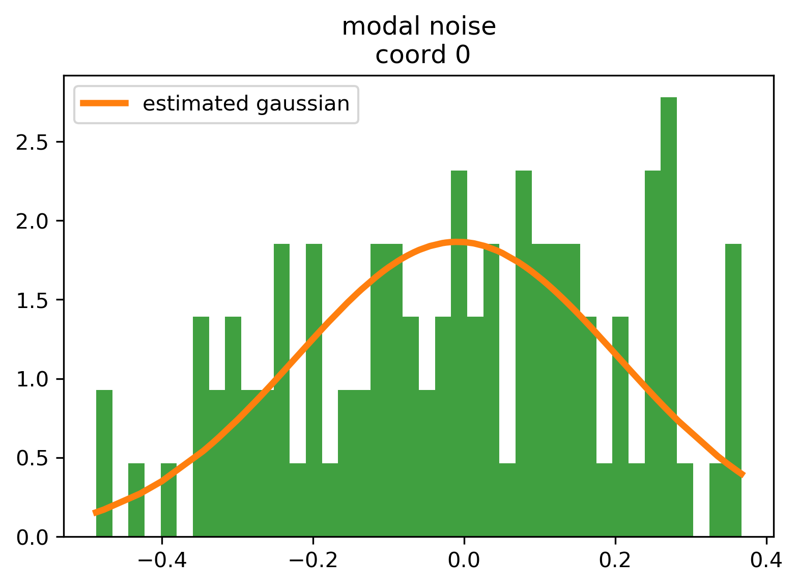
(c) 30 modes

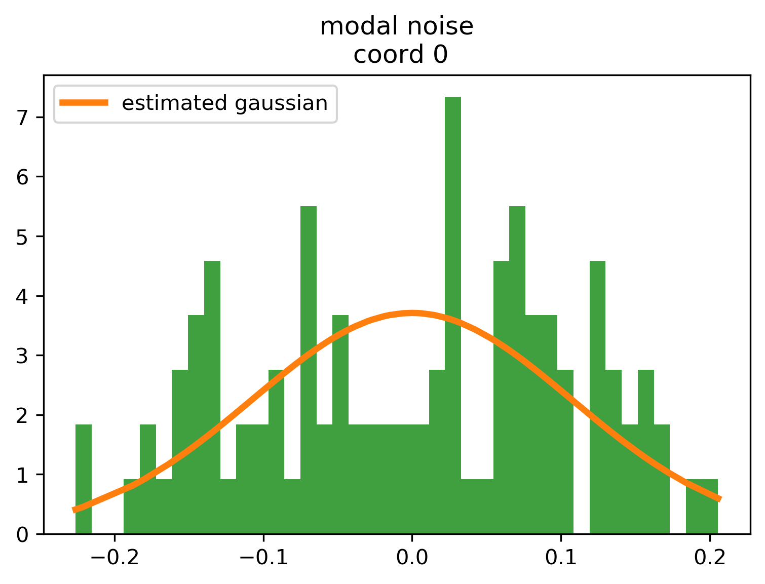
(d) 40 modes

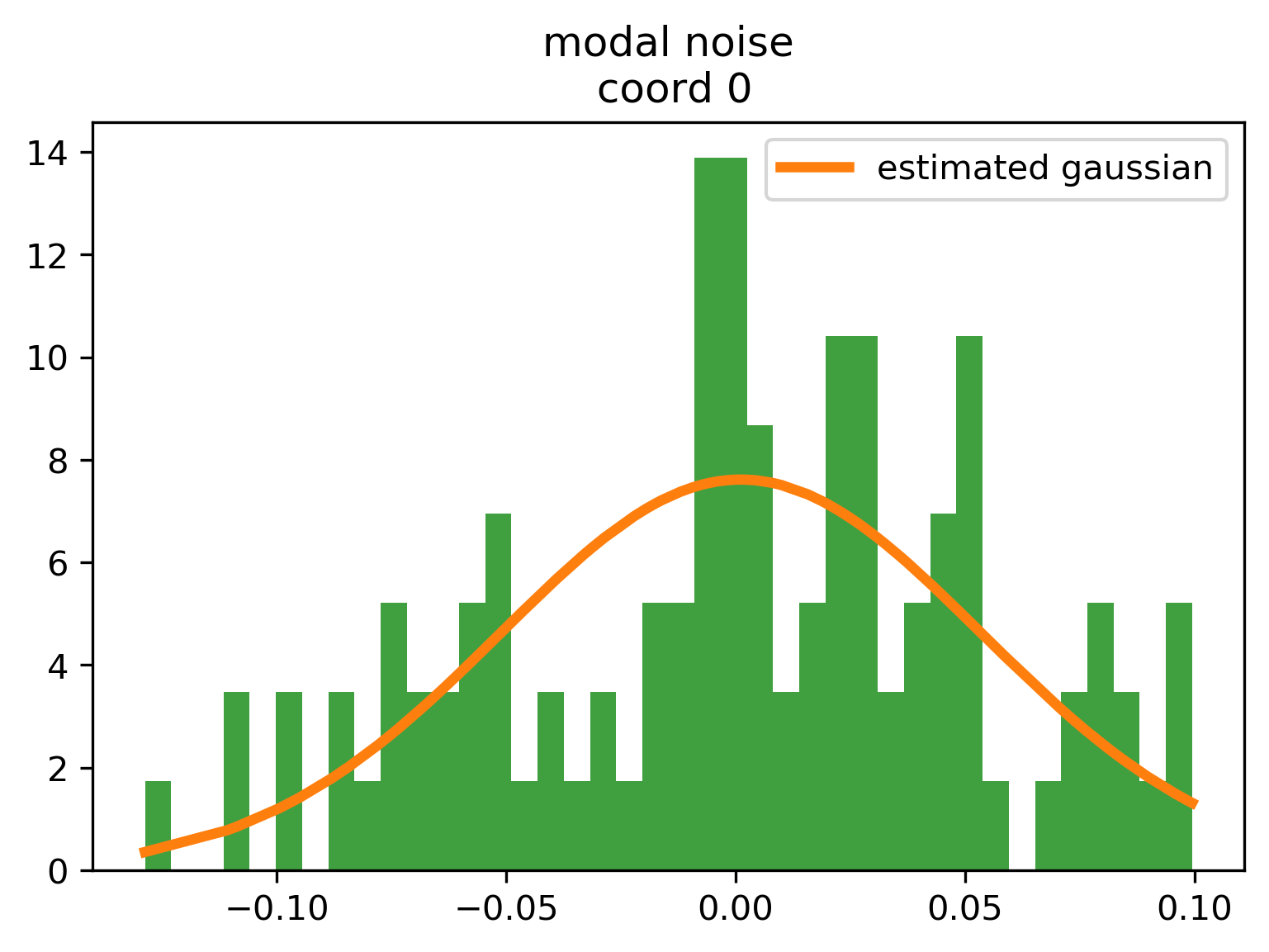
(e) 50 modes

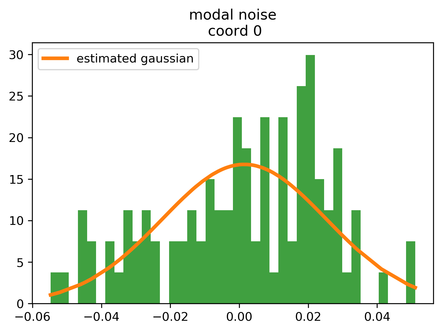
(f) 60 modes

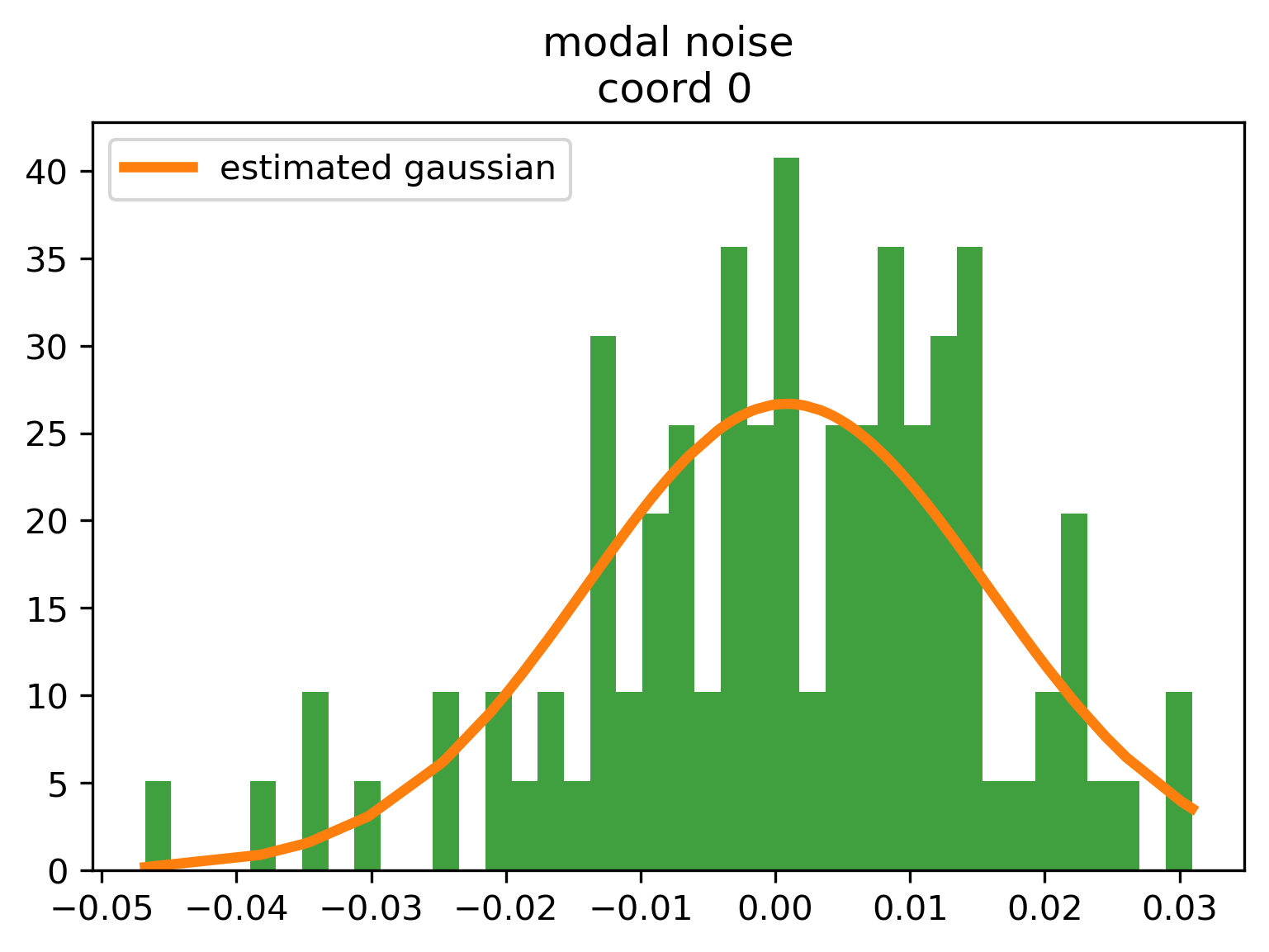
(g) 70 modes

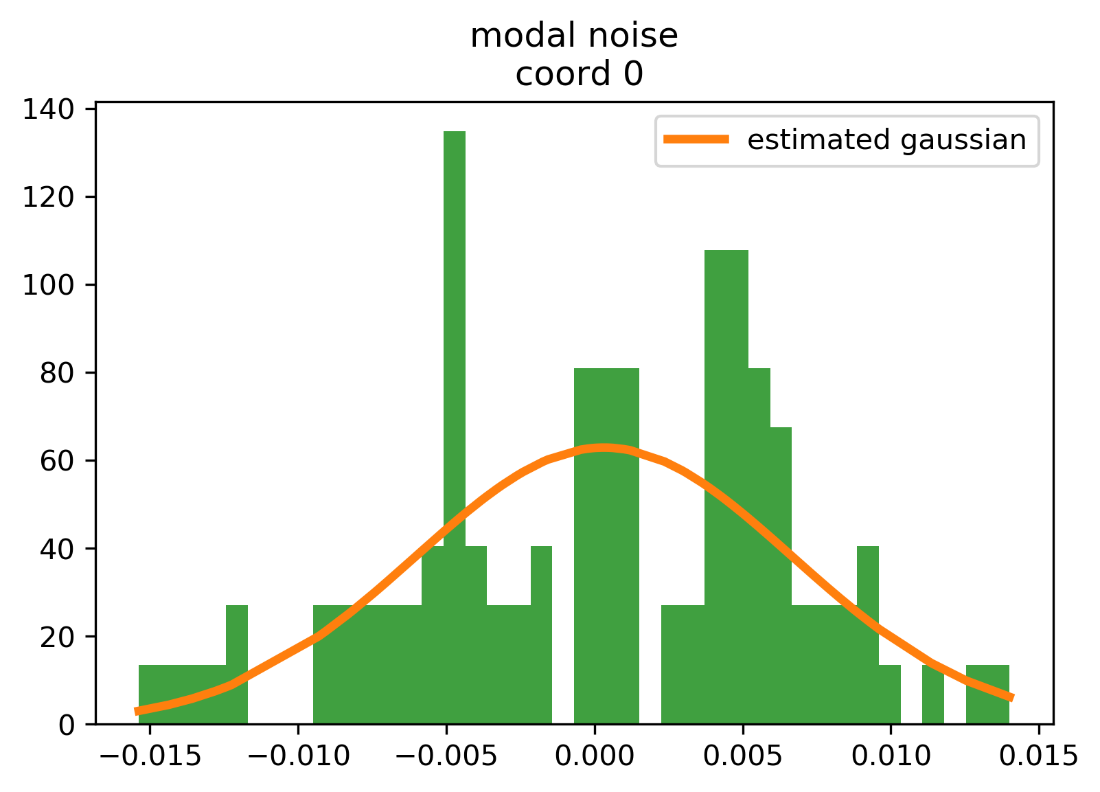
(h) 80 modes

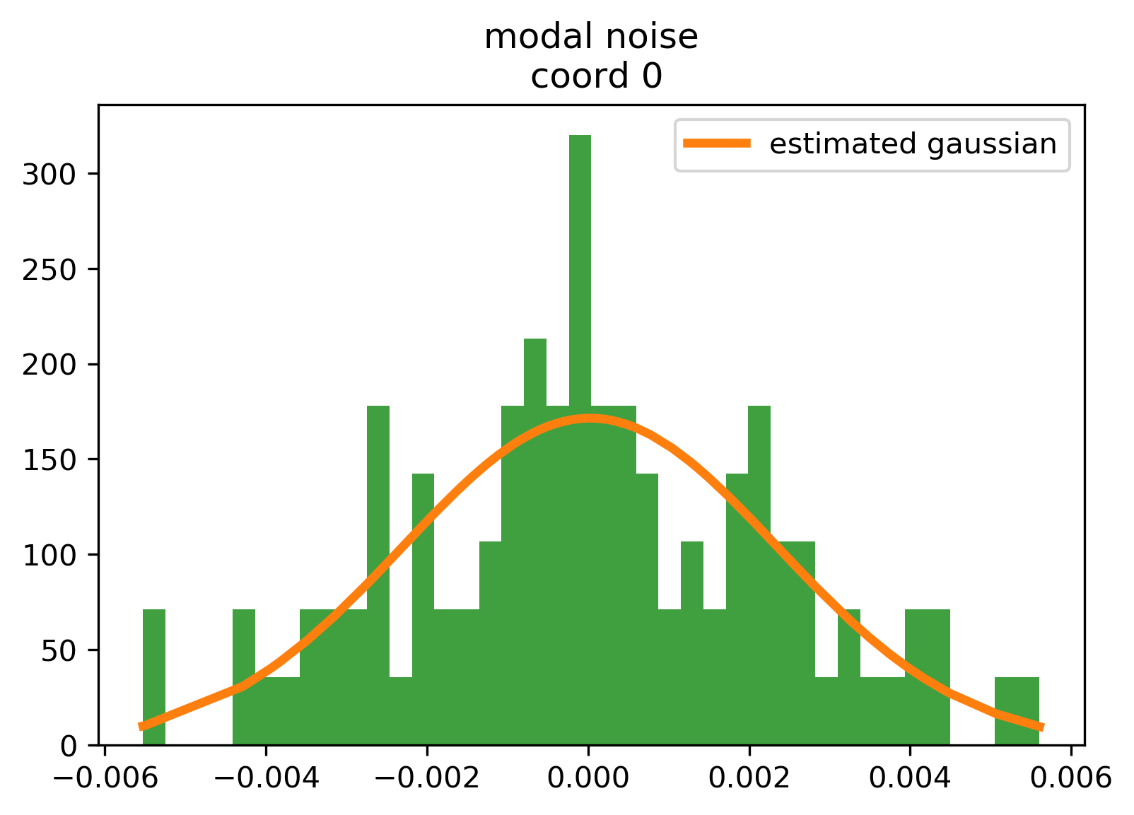
(i) 90 modes

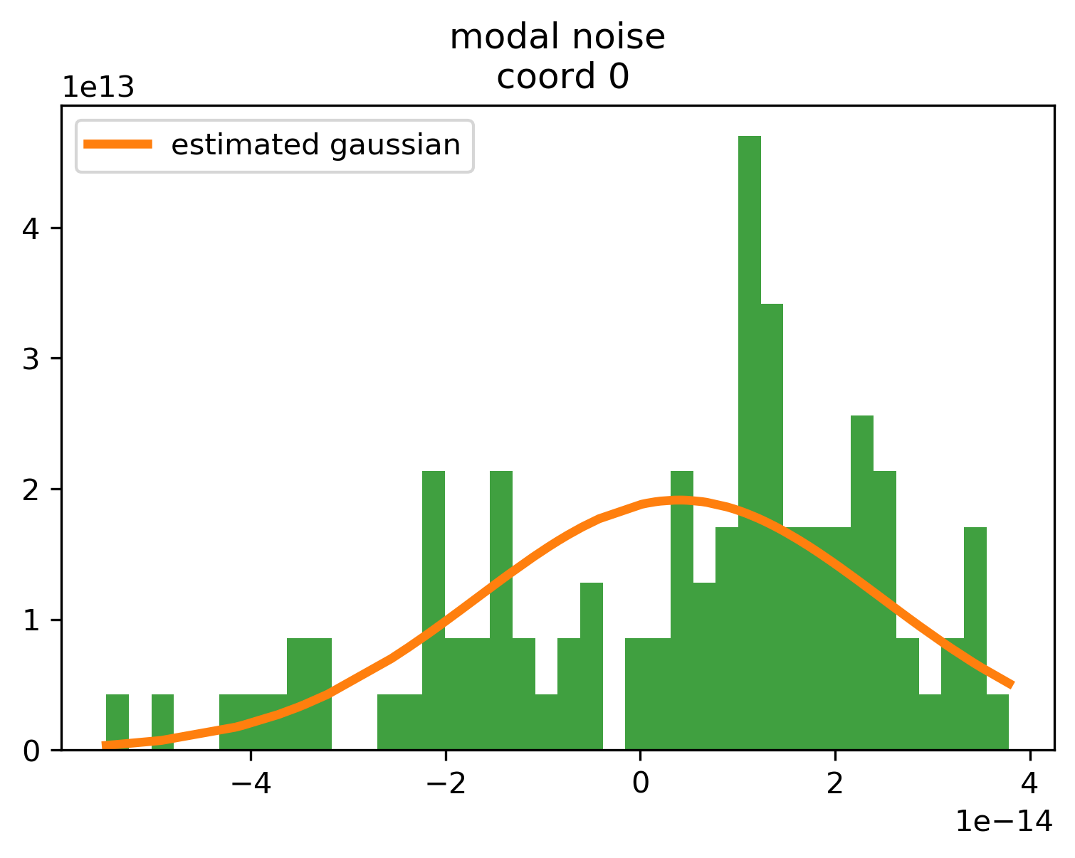
(j) 100 modes

Figure 16: Kuramoto models: Modal noise distributions vs number of modes used for reconstruction.

We quantify the KROM algorithm using two metrics. The first is the reconstruction error. This is simply the average “geodesic” distance between the trajectories. If the true trajectory is $\Theta=\{\theta(t):t\in[0,T],\theta(t)\in[0,2\pi)\}$ and the ROM trajectory is $\Phi=\{\phi(t):t\in[0,1,\dots,T],\phi(t)\in[0,2\pi)\}$, then the “geodesic” distance between the trajectories is computed as

(36) $$d(\Theta,\Phi)=\frac{1}{T+1}\left(\sum_{t=0}^{T}\lvert e^{i\theta(t)}-e^{i\phi(t)}\rvert^{2}\right)^{1/2}.$$

Note this is not the true geodesic distance for $[0,2\pi)\mod 2\pi$, computed as

(37) $$d_{g}(\theta,\phi)=\min_{k\in\mathbb{Z}}\lvert\theta+(2\pi k+\phi)\rvert,$$

but is a good approximation.

Fig. 17 shows the natural logarithm of the reconstruction errors for each oscillator, parameterized by the number of modes used for reconstruction. The error between the signal and the ROM is a smoothe function of the number of modes used for reconstruction. There is (generally) a significant decrease in the log error with increasing number of modes.

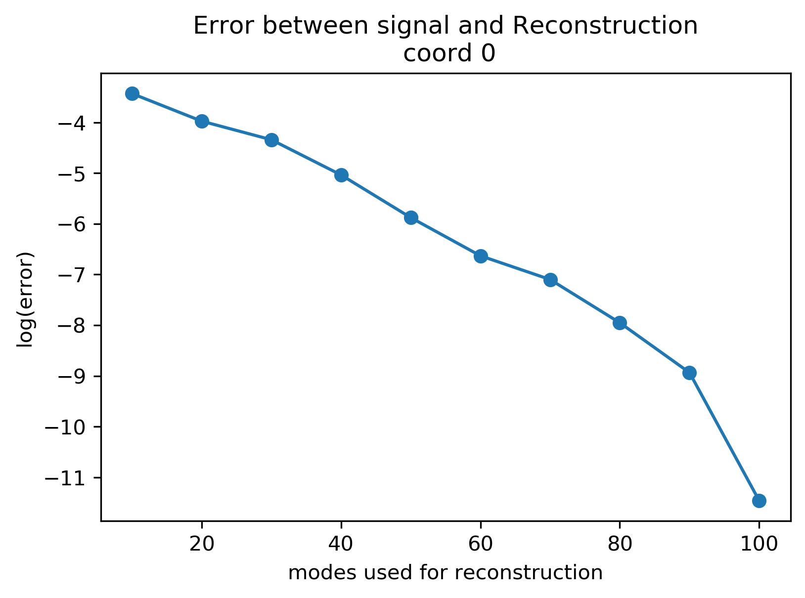
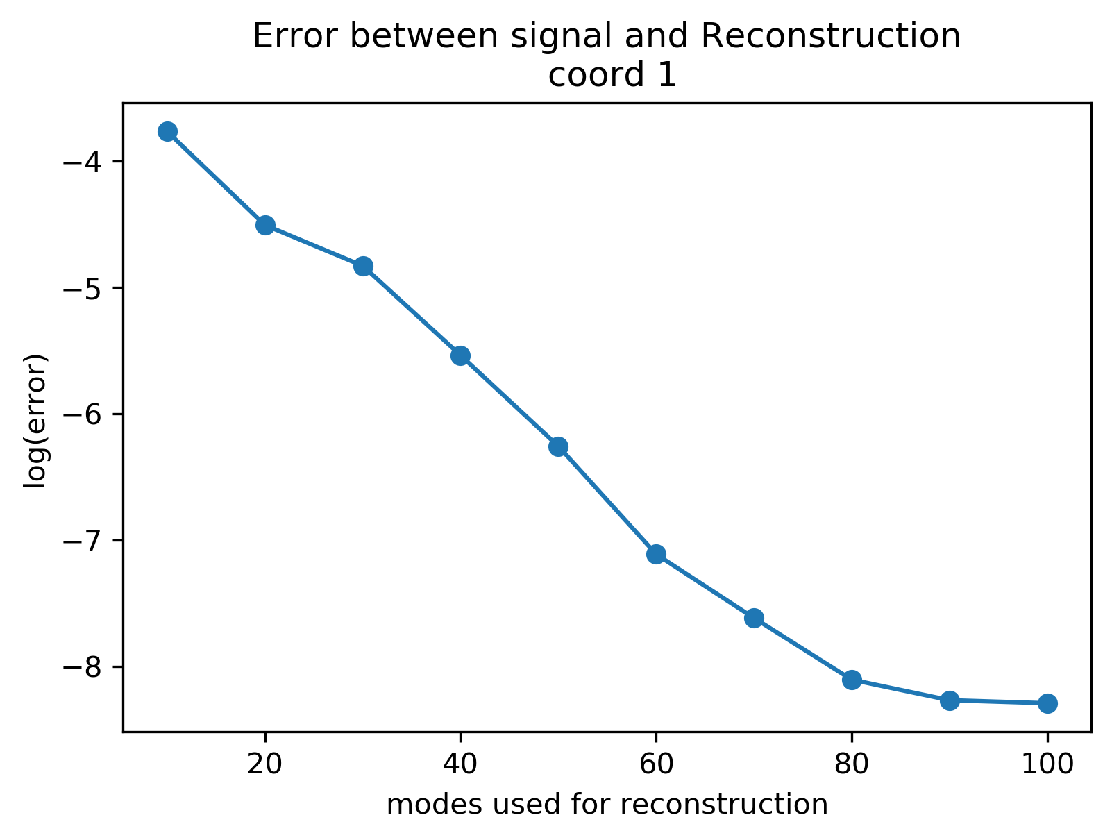
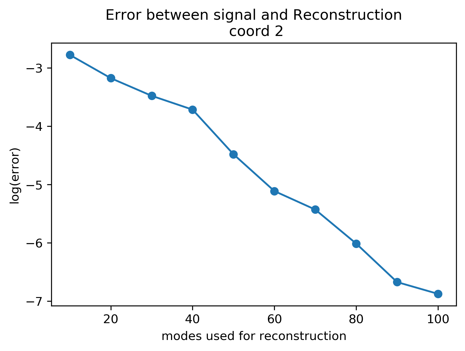
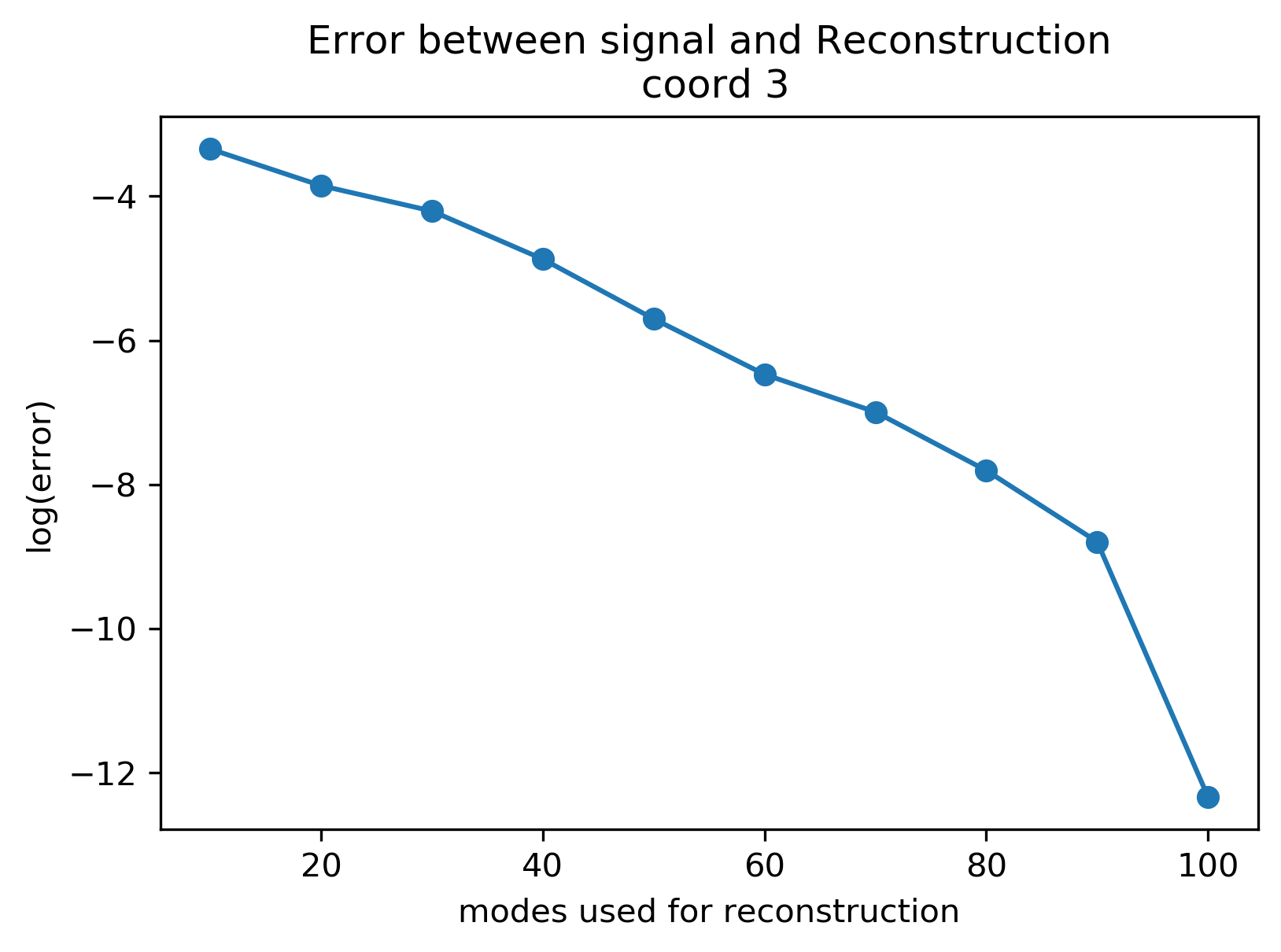
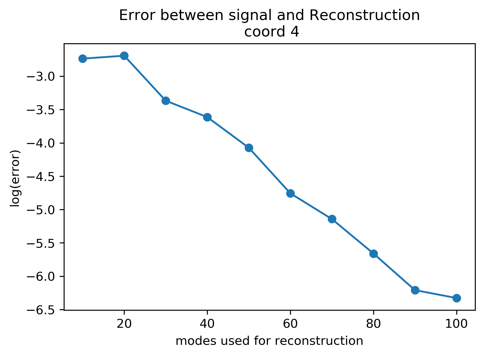
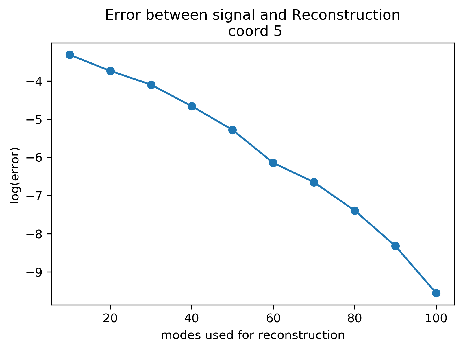
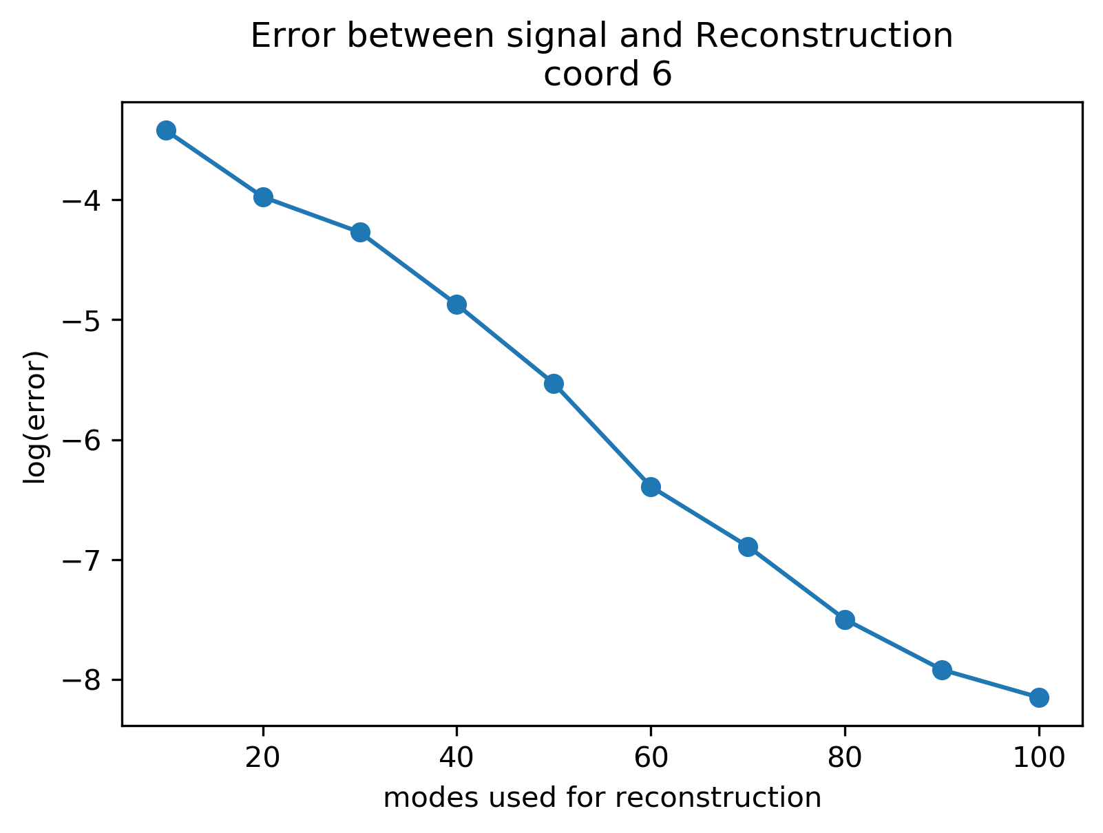
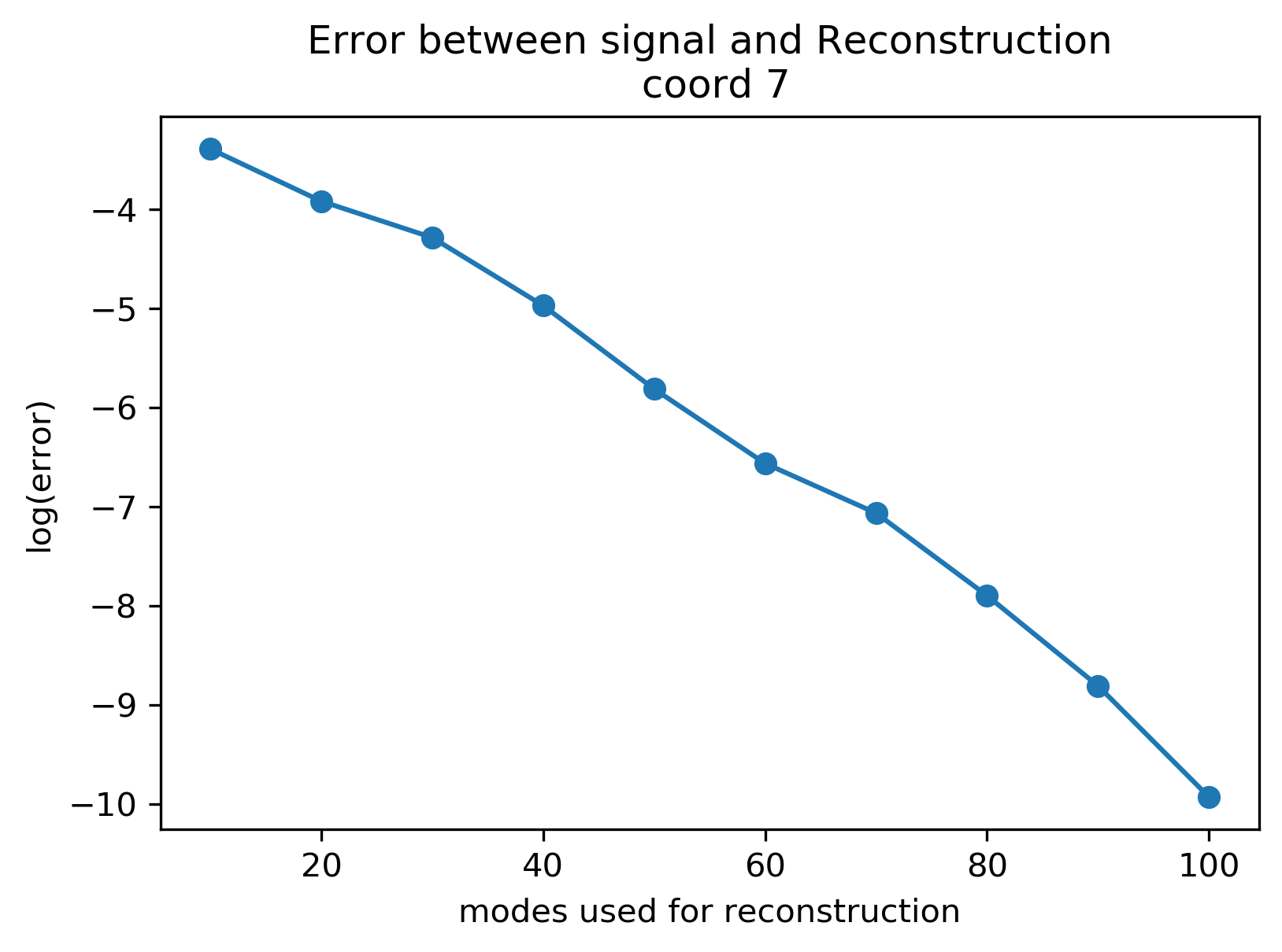
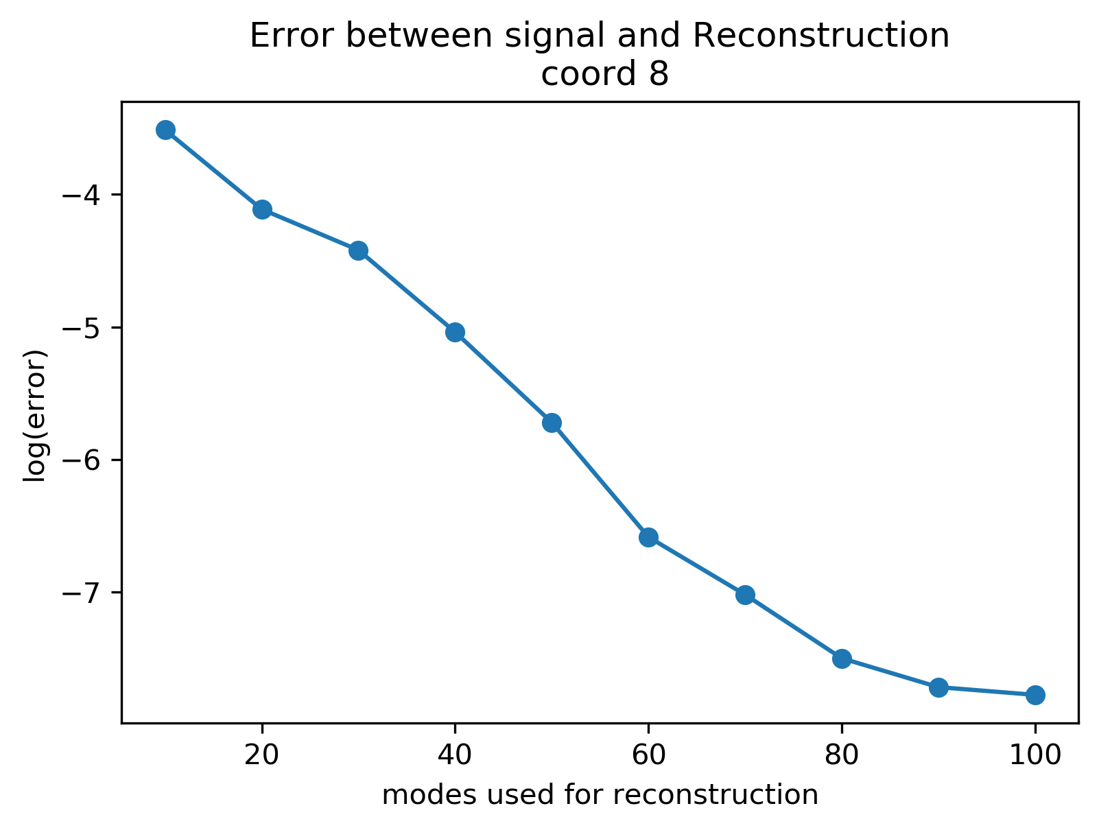
Figure 17: Kuramoto models, signal vs reconstruction error: Comparison of error between the reconstruction signal and the true signal for each oscillator. The reconstruction error is computed using (36).

While the log error between the signal and the reduced order model is a good metric, we also have access to the modal noise which we use to put error bounds on the predictions given by the ROM. We compute the percentage of time the true trajectory is within $\pm 2$ standard deviations of the ROM’s prediction. This is computed as

(38) $$P=\frac{1}{T+1}\sum_{t=0}^{T}\mathbb{I}_{[0,2\sigma)}(d_{g}(\theta(t),\phi(t)))$$

where $d_{g}(a,b)$ is the true geodesic distance on $[0,2\pi)\mod 2\pi$ and $\sigma$ is the modal noise standard deviation.

Even when using a lower number modes to construct the model (50 modes or less), the ROM shows good residence times, (38), for most of the oscillators. With higher numbers of modes, the residence times remain above $0.8$. One thing to note is that the residence time is not monotonic with respect to the number of modes used for reconstruction. We see non-monotonic behavior for models utilizing 50 modes up to 100 modes (full reconstruction). We believe part of this is due to the way the standard deviation of the modal noise is computed. The modal noise is computed using the residual between the signal and the reconstruction. As a consequence, as the reconstruction becomes more accurate, the variance of the residual sequence reduces. As can be seen, especially in Fig. Fig. 16, the standard deviation in the modal noise rapidly tightens as the number of modes increases. This may account for the non-monotonic behavior. A true analysis requires computing the rate of decrease in the variance of the modal noise versus the number of modes used for reconstruction contrasted with the rate of reduction of the error between the signal and the reconstruction with respect to the number of modes used for reconstruction.

Fig. 17 shows the reconstruction error of the ROM’s vs. the number of modes used for reconstruction. Fig. 18 shows the fraction of time that the true signal is within 2 standard deviations of the ROM prediction.

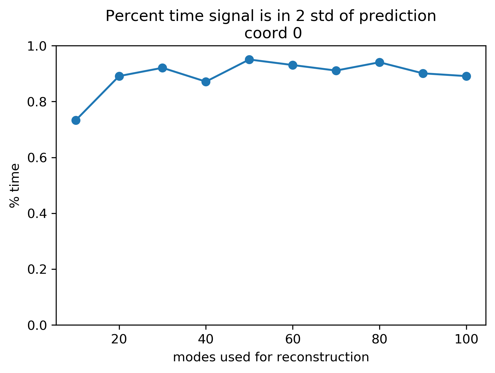
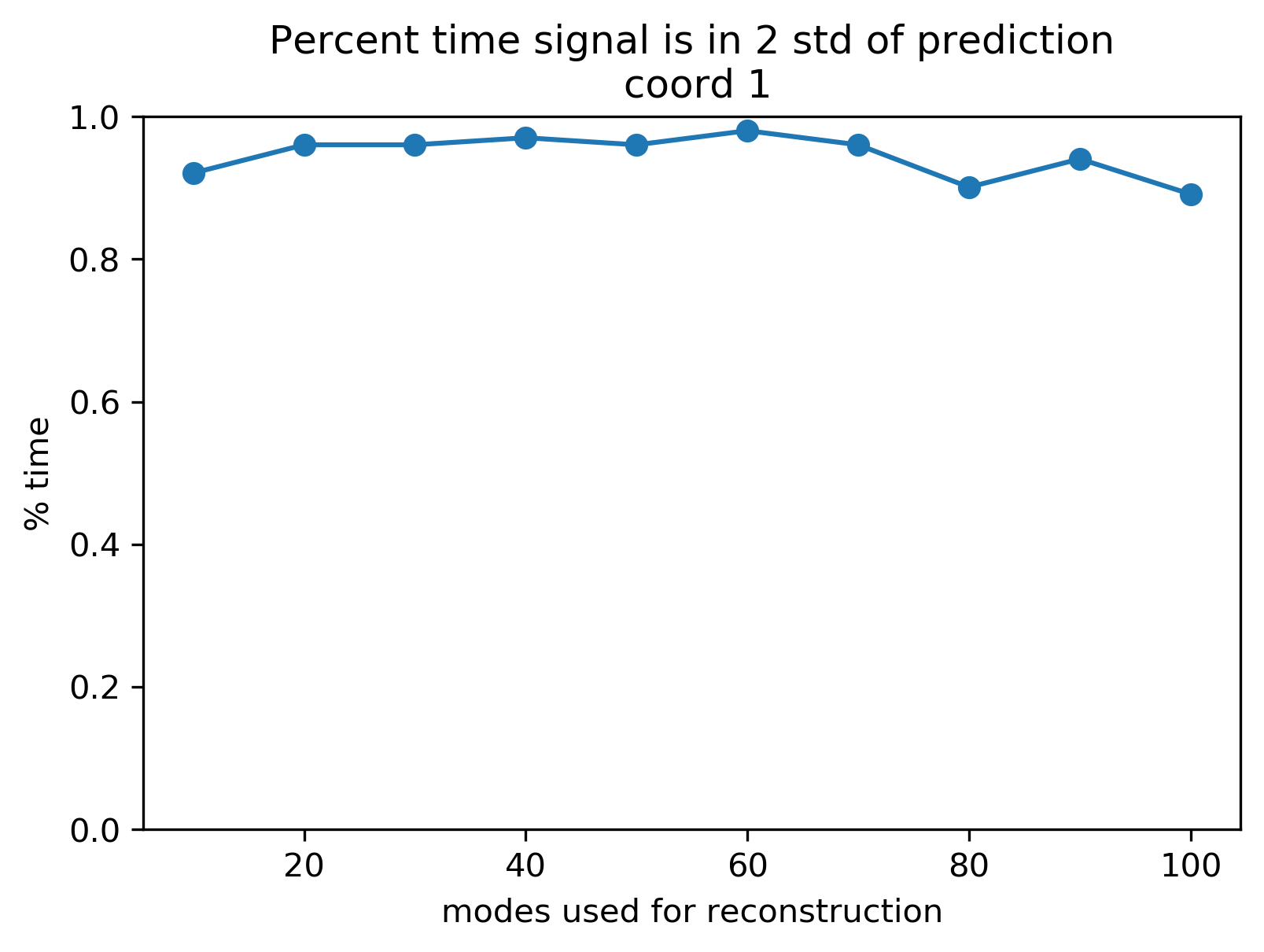
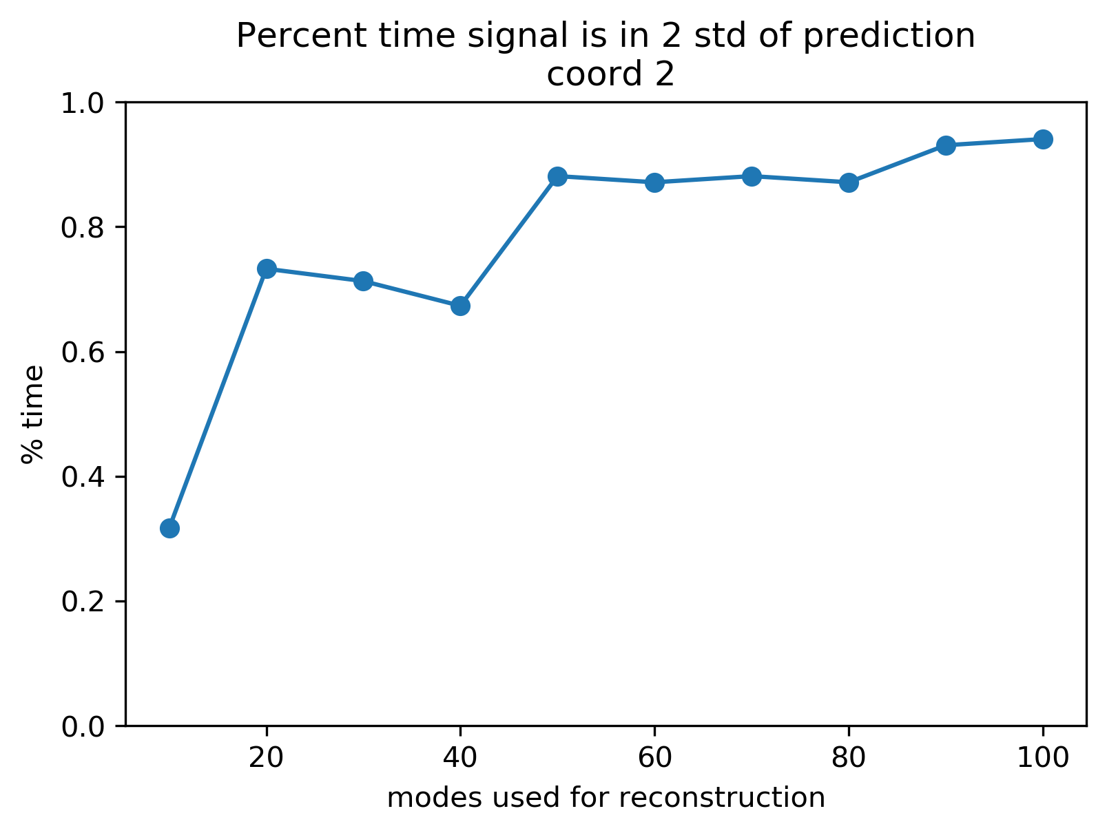
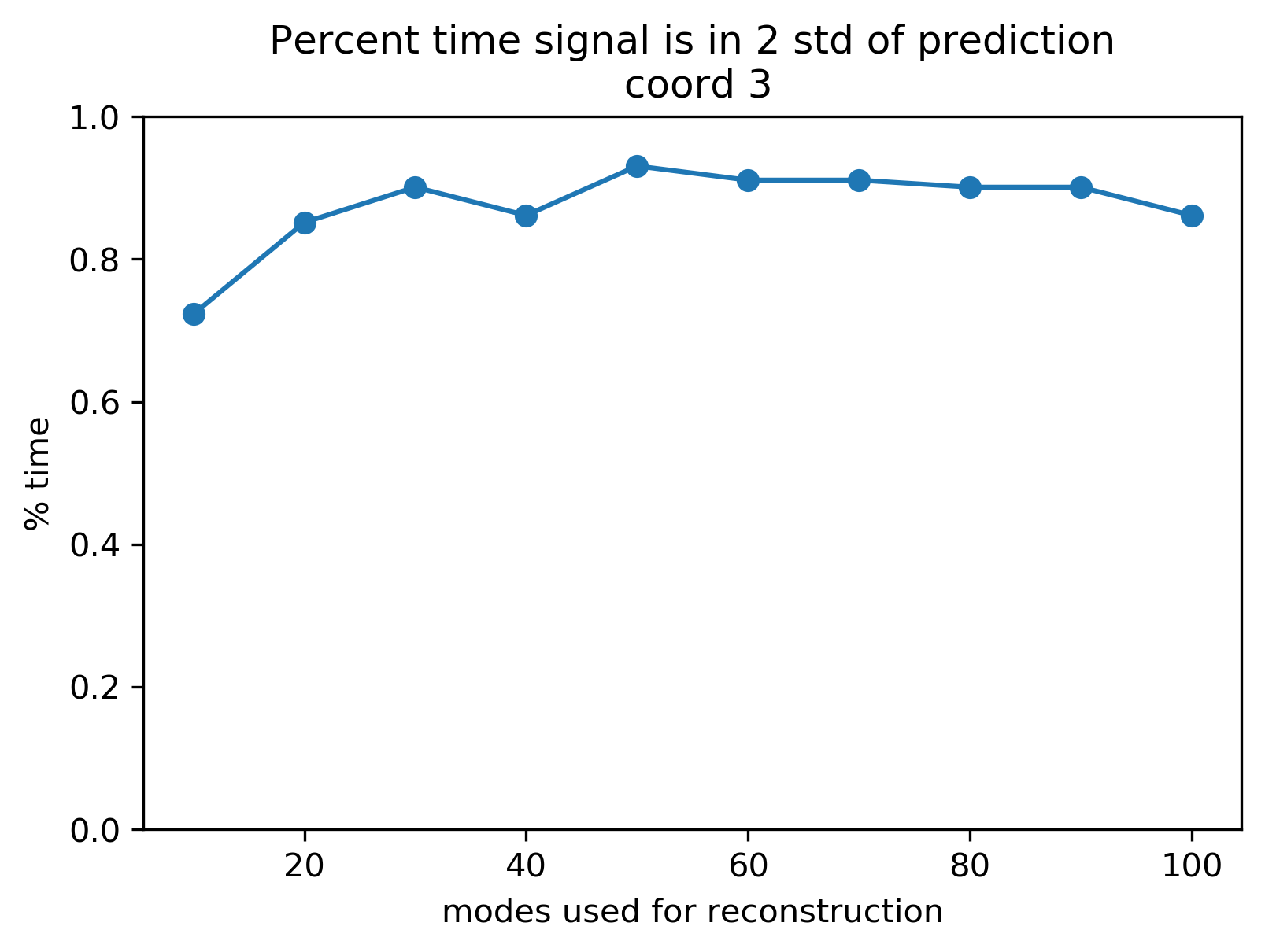
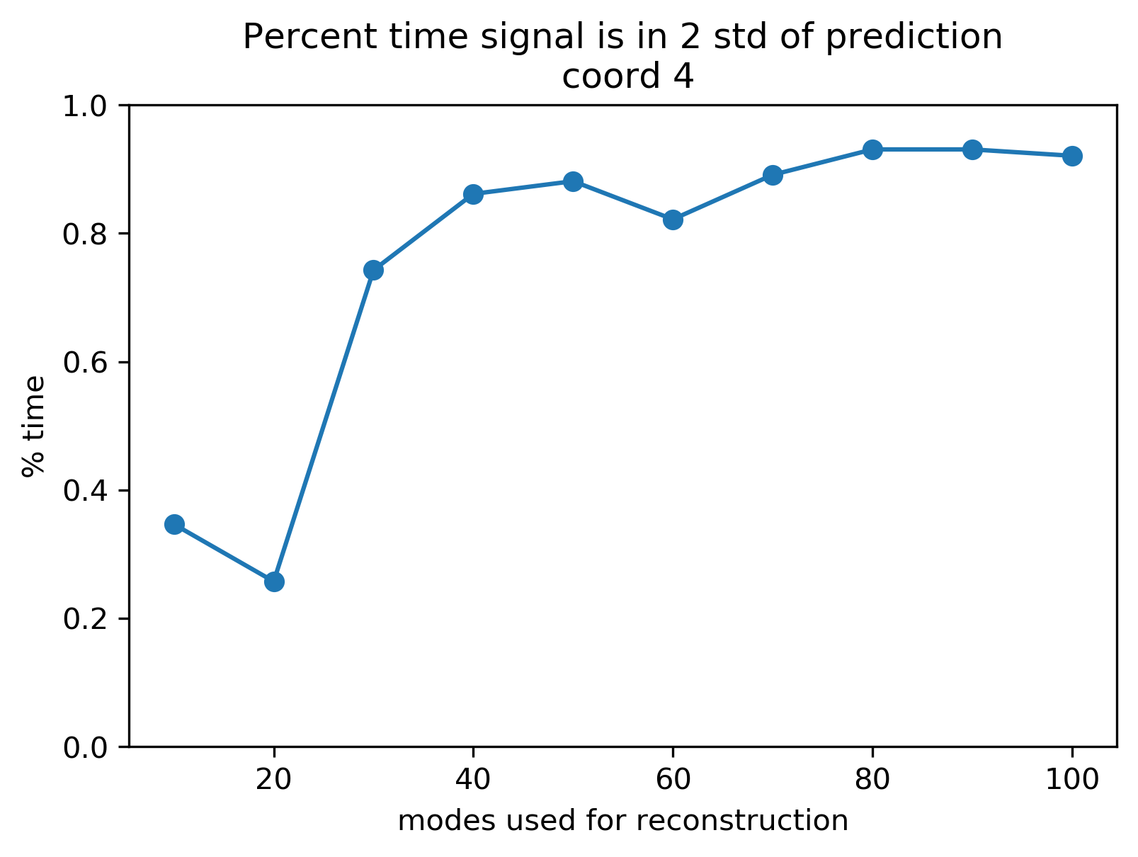
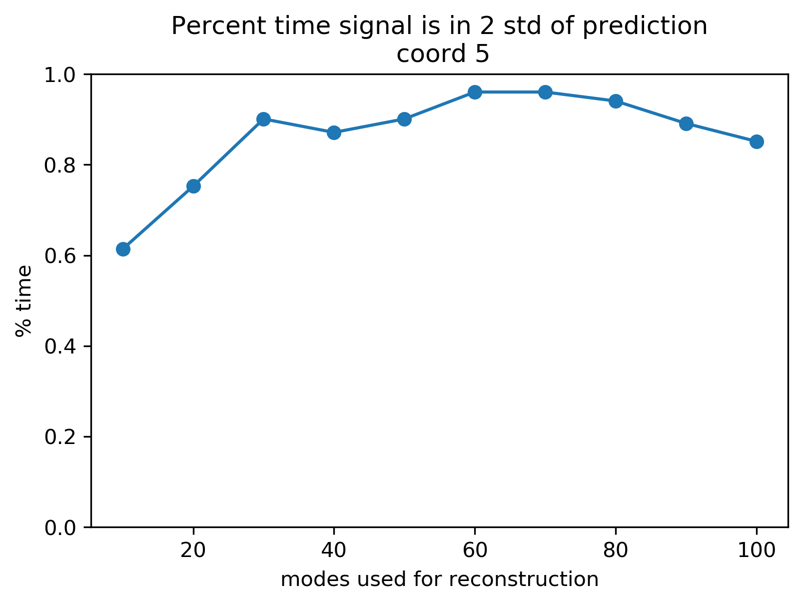
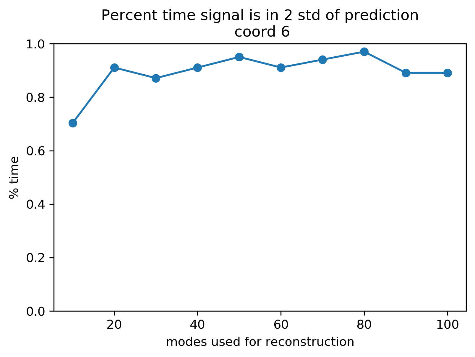
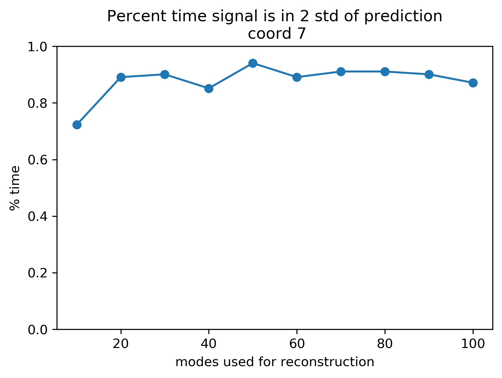
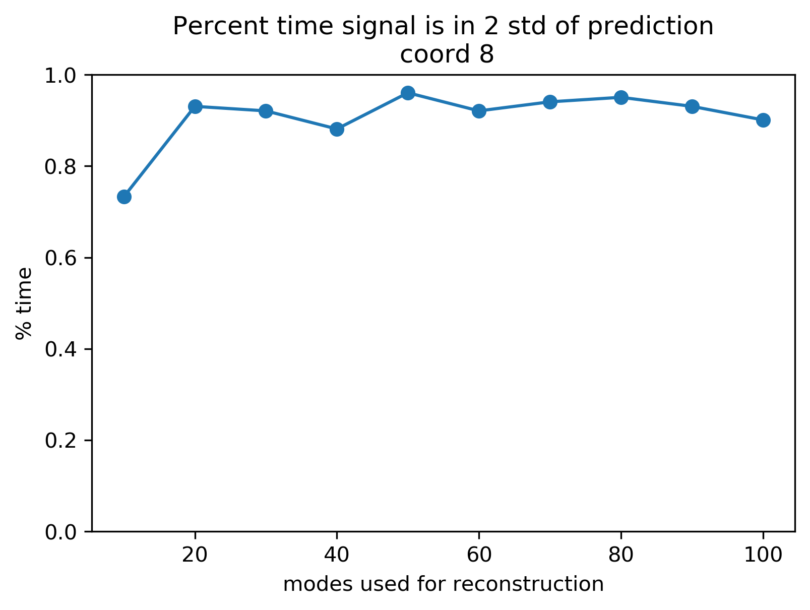
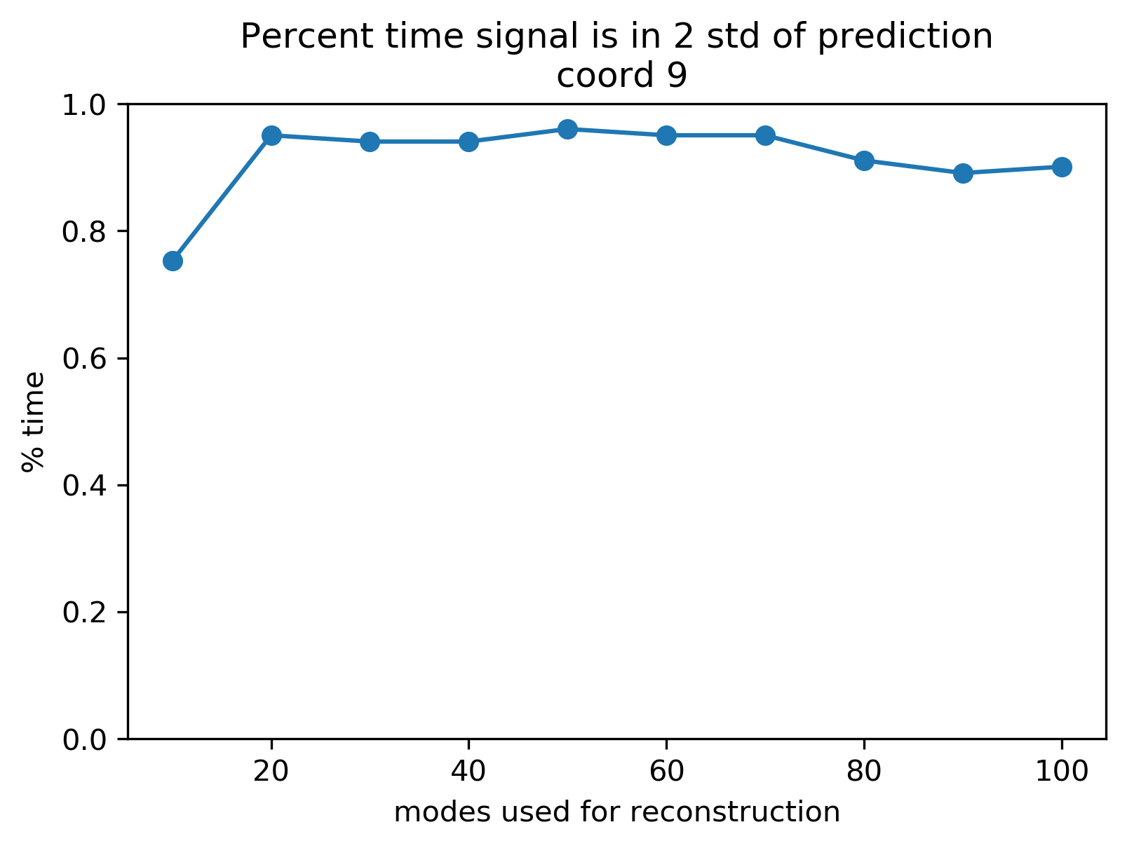
Figure 18: Kuramoto models, percent time signal is within $\pm 2$ standard deviations of ROM signal: Residence times in $\pm 2$ standard deviation band is computed via (38).

4 A heuristic for estimating the minimum number of modes to use for the ROM

Above, we have computed a sequence of reduced order models for 3 examples, from a minimum of 10 modes up to a full reconstruction (100 modes in all examples). The question remains how to choose the final number of modes to be used in the reduced order model (ROM); too few and the we get poor prediction accuracy, too many results in a larger and more expensive model.

In this section, we present a heuristic method to determine the minimum number of modes that must be taken. This method is based on testing the normality of the modal distribution that is computed for each ROM. The rationale is as follows. In our examples, we have structured dynamics plus added noise and a changing network topology. When we construct our model, we compute a deterministic model and then estimate the modal noise distribution. We assume that once we have adequately recovered the true structured dynamics with the computed deterministic model the modal noise will have a Gaussian distribution. If too few modes are used for the deterministic model, much of the structured part of the dynamics will be modeled as noise, destroying the normality of the modal distribution. By using too many modes in the deterministic model, the noisy part of the dynamics are subsumed into a deterministic model, possibly destroying the normality of the distribution.

Algorithm 3 specifies the heuristic. We note that this test can be computed automatically and does not require manually looking at histograms or quartile-quartile plots to determine this although we show such plots in Fig. 19, Fig. 20, and Fig. 21 below. In each of the figures, panel (a) shows both the mean and median p-values vs. the number of modes. Panel (b) shows a box a whisker plot of the p-values to show their distribution. Panel (c) shows a quartile-quartile plot; the closer the blue dots follow the red line, the closer the distribution is to a normal distribution. Final, panel (d) shows the reduced order model reconstruction using the number of modes dictated by the heuristic algorithm.

Algorithm 3 Heuristic for determining the minimum number of modes used in the ROM

  Input Data: The set modal noise distributions $\rho_{i}$ for model $i$.

  1: Let $\rho_{i}=\{\rho_{i,j}\}_{j=1}^{J}$ be the set of modal distributions for reduced order model $i$. $\rho_{i,j}$ is the modal distribution for the $j$-th coordinate of the system. The $\rho_{i}$’s should be ordered from smallest model to largest (e.g., $i=10,20,\dots,100$ in our examples.)

  2: For $j=1,\dots,J$, perform a Shapiro-Wilkes hypothesis test to compute $J$ p-values, $p_{i}=\{p_{i,1},\dots,p_{i,J}\}$ (one for each modal distribution).

  3: For each $i$, compute the mean and median of the set $p_{i}$.

  Heuristic: The smallest ROM where both the mean and median are above 0.05 is the smallest number of modes one should take for the model.

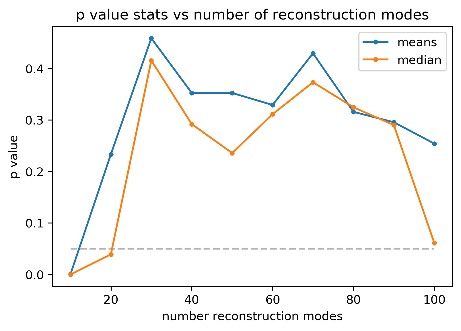
(a) p values mean, median

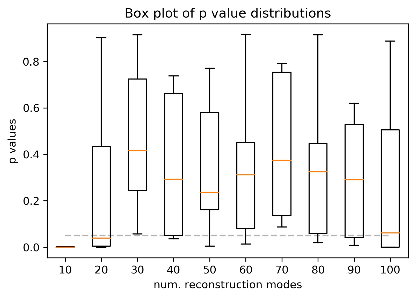
(b) p values boxplot

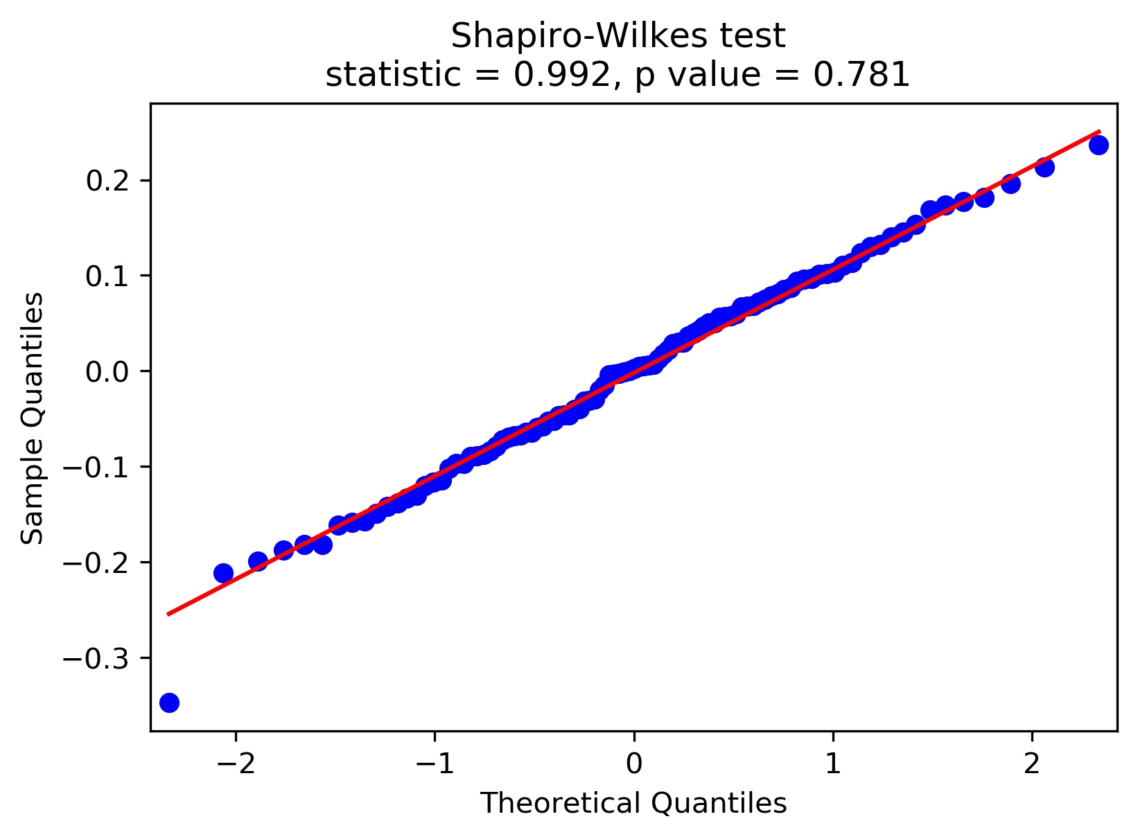
(c) quartile-quartile plot of coordinate 0’s modal distribution.

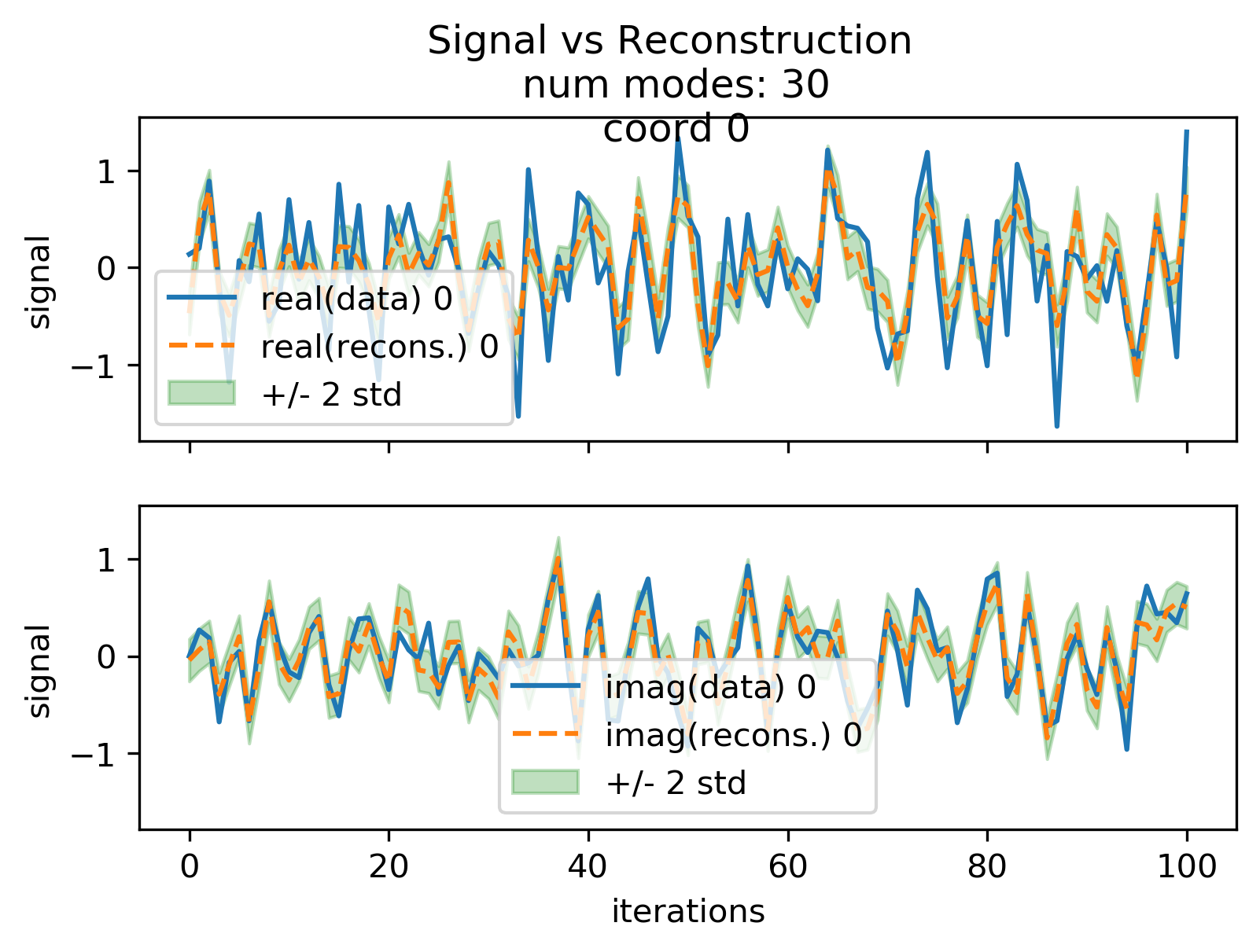
(d) 30 mode reconstruction of coordinate 0.

Figure 19: Linear modal model’s p-values: Pane (a) shows a visual representation of the outputs of the heuristic, namely the mean and median p values for the different sizes of models. The heuristic says that 30 modes is the minimum number to use for the ROM. (b) is similar except it is a boxplot of the modal distributions’ p values. (c) quartile-quartile plot for coordinate 0’s modal distribution visually testing for normality. (d) coordinate 0’s reconstruction with the 30 mode ROM.

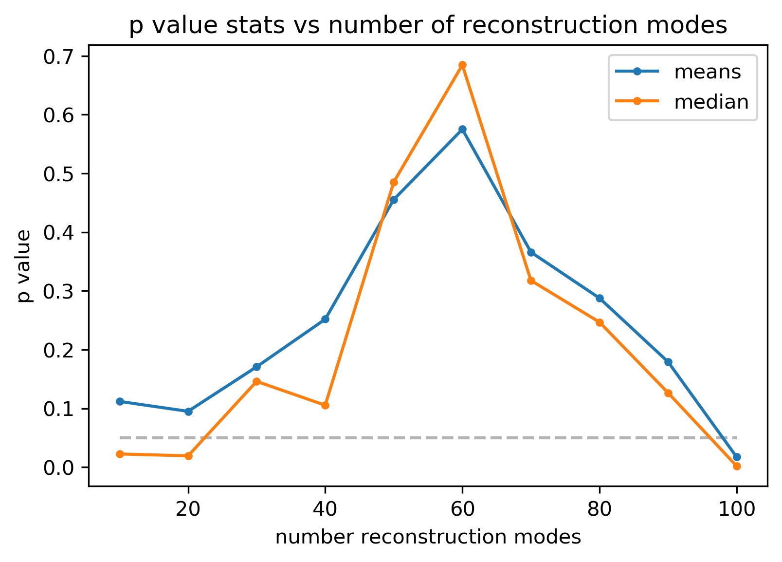
(a) p values mean, median

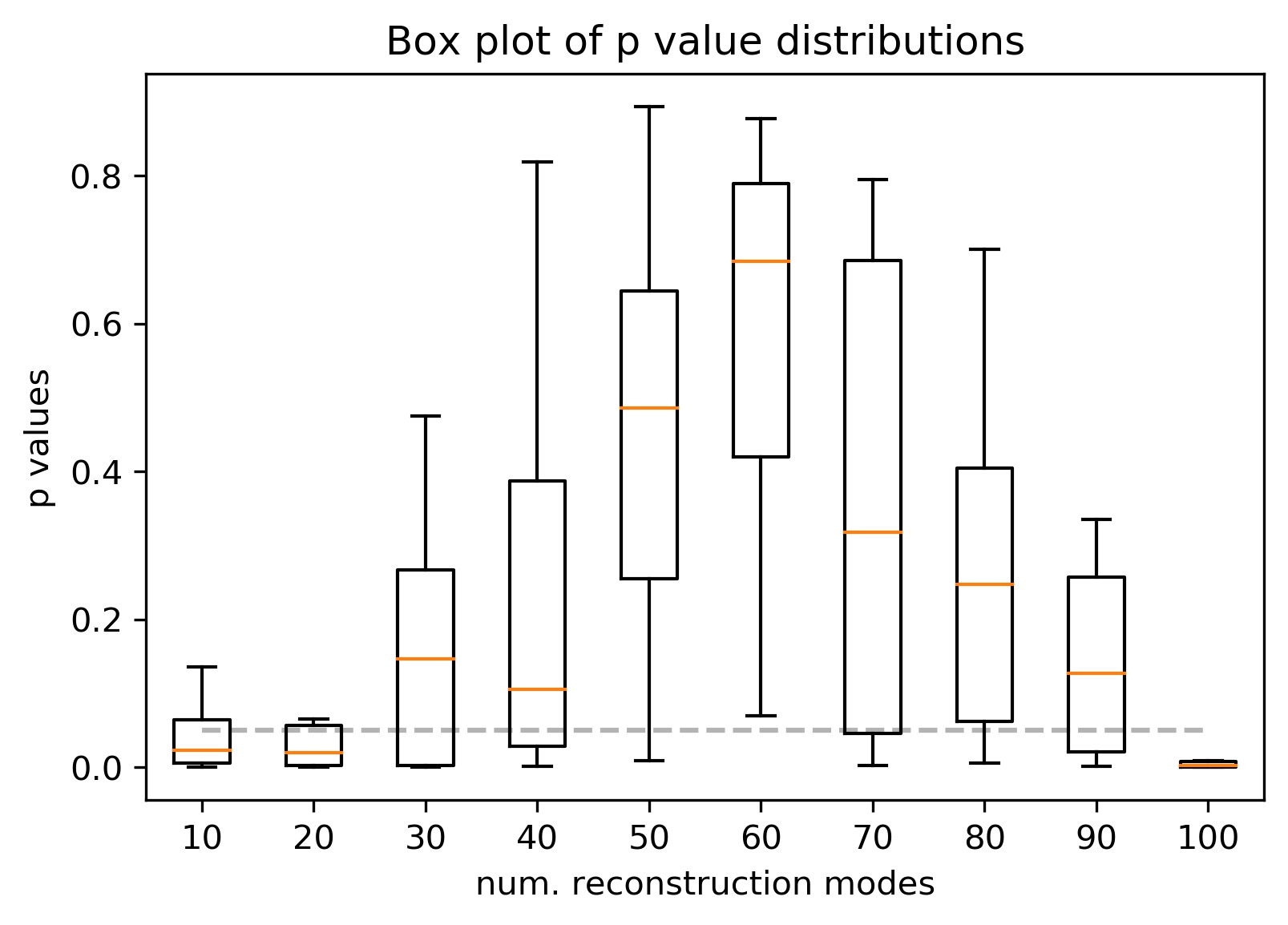
(b) p values boxplot

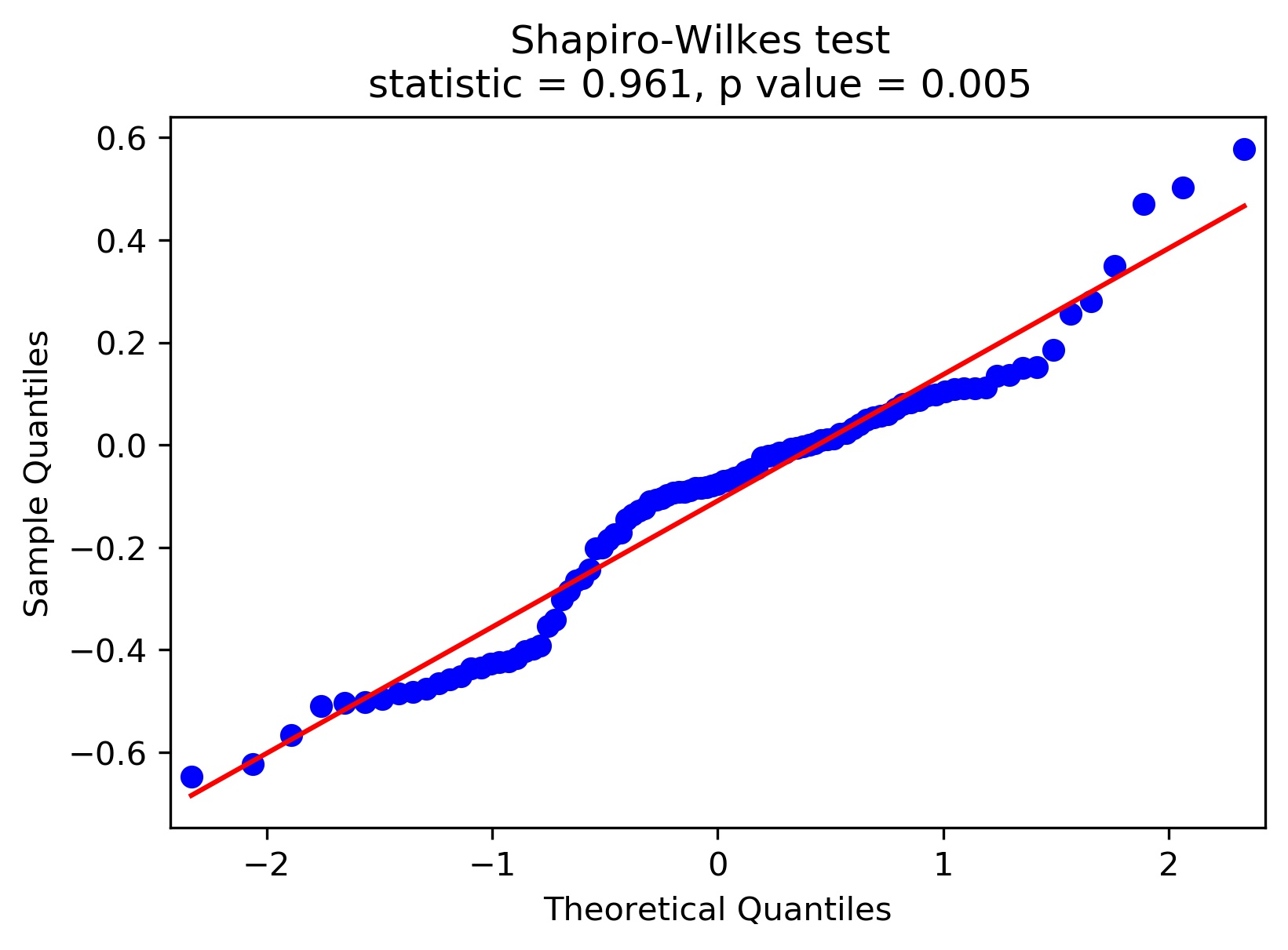
(c) quartile-quartile plot of coordinate 0’s modal distribution.

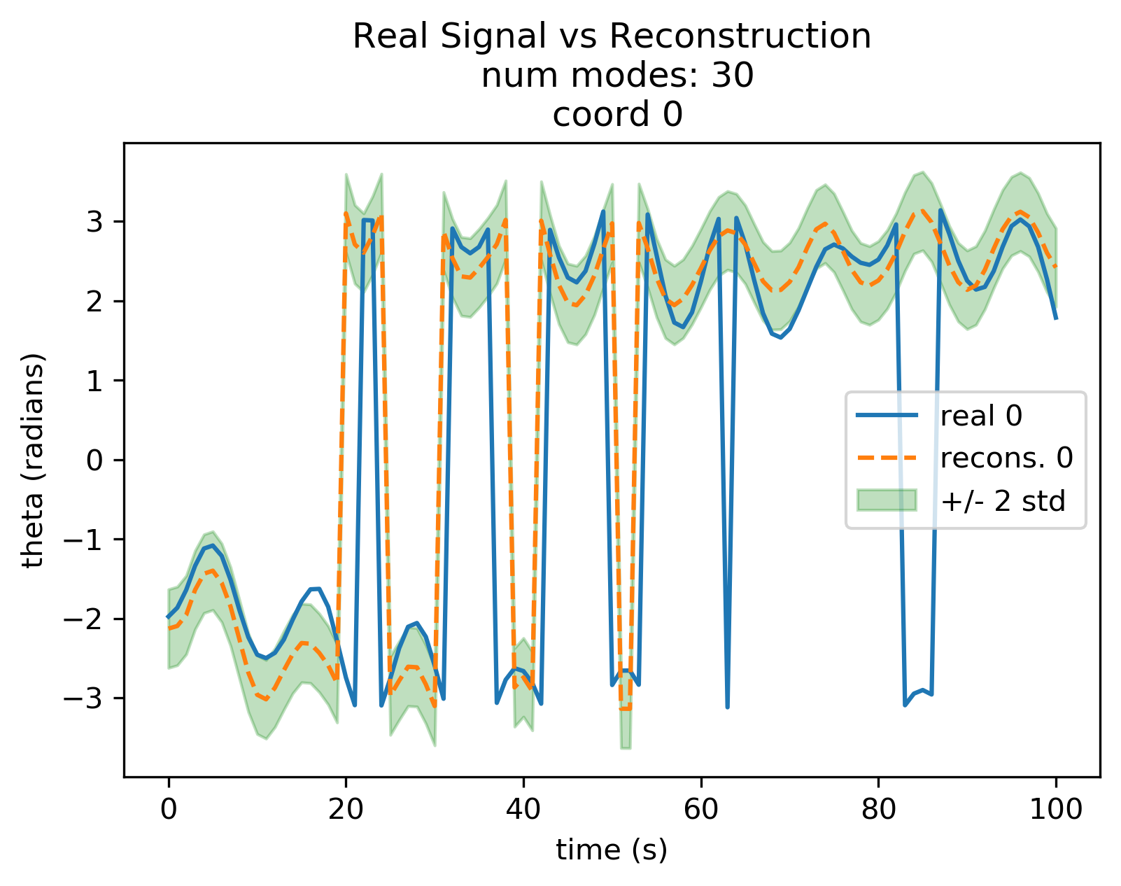
(d) 30 mode reconstruction of coordinate 0.

Figure 20: Kuramoto model’s p-values: In (a) be show a visual representation of the outputs of the heuristic, namely the mean and median p values for the different sizes of models. The heuristic says that 40 modes is the minimum number to use for the ROM. (b) is similar except it is a boxplot of the modal distributions’ p values. (c) quartile-quartile plot for coordinate 0’s modal distribution visually testing for normality. While the mean and median of the p values are above the 0.05 threshold, this particular coordinate is not approximated well by a normal distribution. (d) coordinate 0’s reconstruction with the 30 mode ROM.

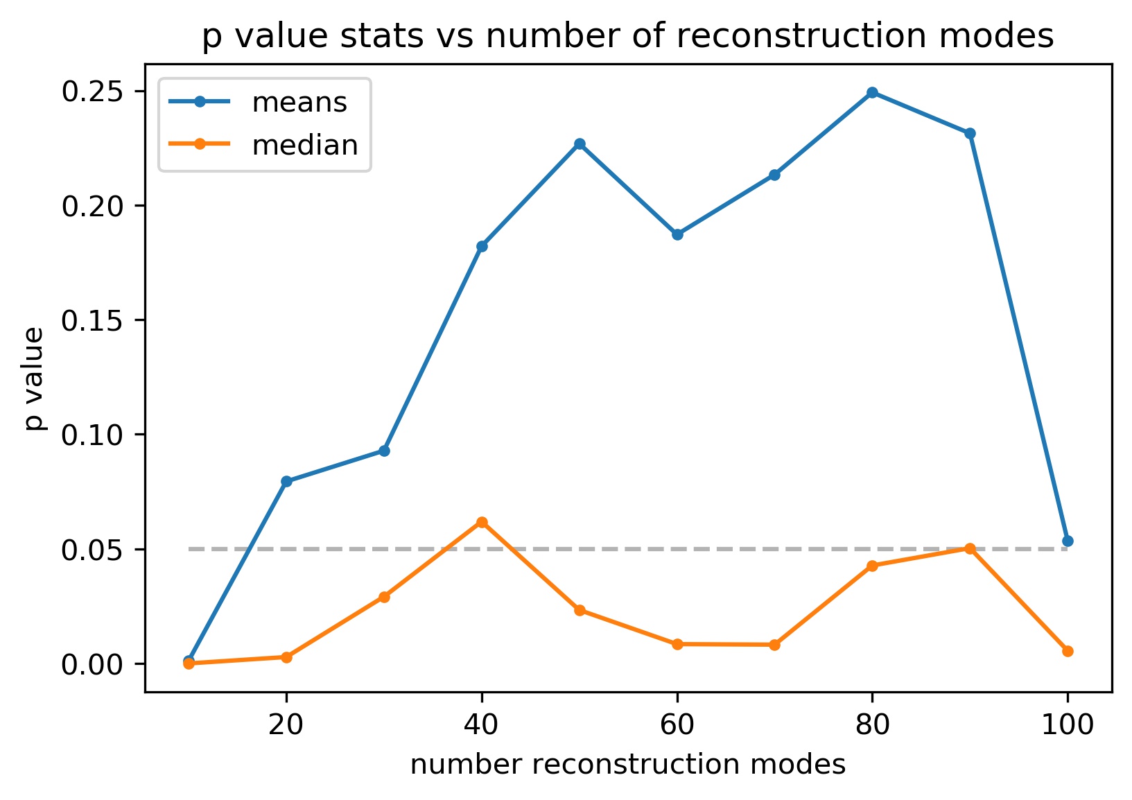
(a) p values mean, median

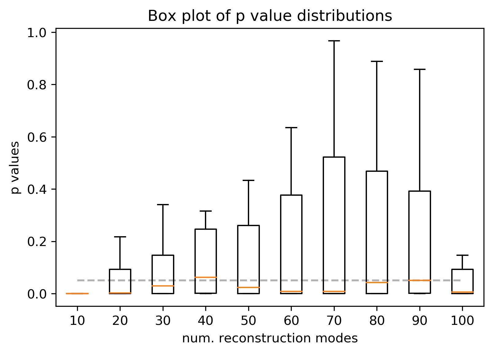
(b) p values boxplot

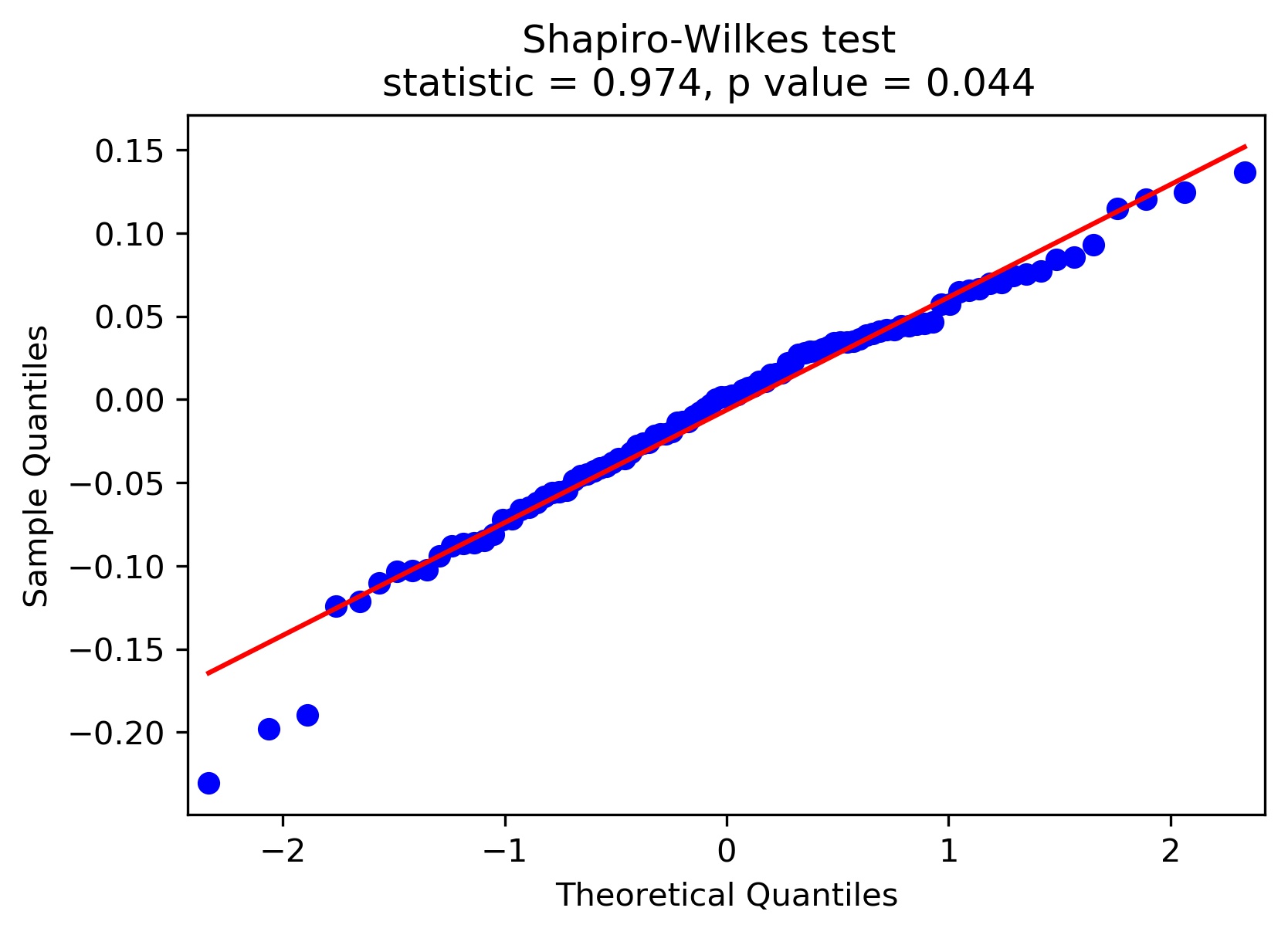
(c) quartile-quartile plot of coordinate 0’s modal distribution.

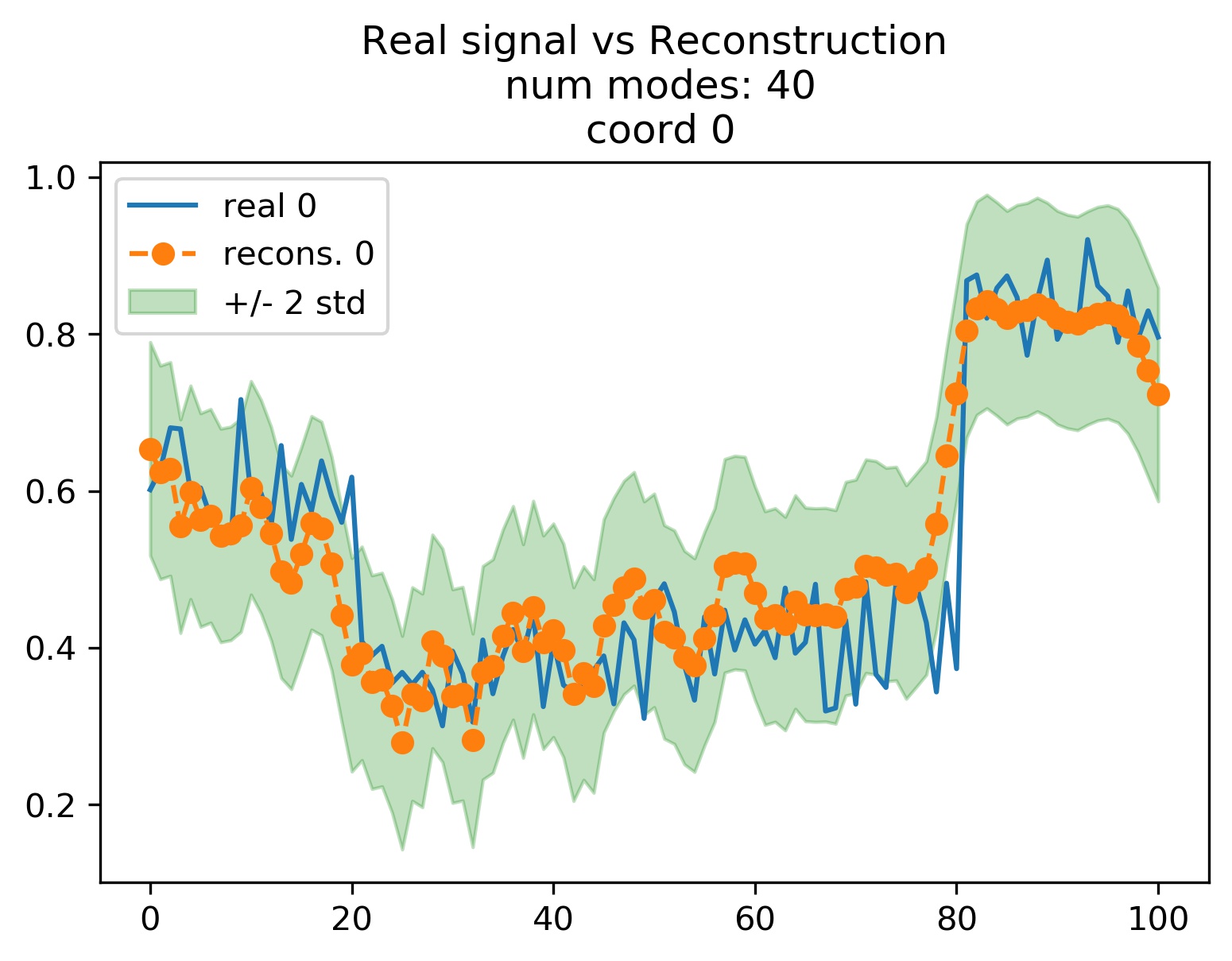
(d) 40 mode reconstruction of coordinate 0.

Figure 21: Anharmonic model’s p-values: Pane (a) shows a visual representation of the outputs of the heuristic, namely the mean and median p values for the different sizes of models. The heuristic says that 30 modes is the minimum number to use for the ROM. (b) is similar except it is a boxplot of the modal distributions’ p values. (c) quartile-quartile plot for coordinate 0’s modal distribution visually testing for normality. (d) coordinate 0’s reconstruction with the 40 mode ROM.

5 Discussion and Conclusions

We have developed a method for reduced order modeling using Koopman operator theory that gives confidence bounds on the predictions of the reduced order model. This is accomplished in the following way. While the reduced order model is by necessity a finite process, the spectral expansion of the Koopman operator is infinite. The reduced order model represents the process with a finite number of Koopman modes. The rest of the dynamics are modeled as a noise process. The part of the noise process that is in the subspace modeled by the ROM’s modes is called the modal process. This noise process is modeled as a Gaussian noise process and the estimated standard deviation of the noise is used to compute a confidence bound on the ROM’s predictions.

We have applied this modeling to a sequence of examples. The first was a synthetic example where we could directly specify the Koopman eigenvalues and modes, so the computed Koopman spectrum could be compared to ground truth. The next two examples represented networked dynamical systems that had changing network topology. The first was a network of noisy, anharmonic oscillators whose connections were switched at each integer time. This system was chosen due to the fact that a single, non-noisy, anharmonic oscillator has a purely continuous spectrum, except the eigenvalue at 1, and thus does not have an expansion in terms of Koopman modes and eigenfunctions. Despite this, the methodology was able to model the system’s evolution with a small number of computed modes plus the noise process. The actual trajectory of the system stayed within the confidence bounds of the ROM’s prediction a large percentage of the time. The last example consisted of a noisy Kuramoto model with random coupling strength between the oscillators. As with the anharmonic oscillator example, the true signal stayed within the confidence bounds of the ROM’s prediction the majority of the time.

In each example there was Gaussian observational noise. As the number of modes increased, we got closer to a deterministic plus Gaussian noise model. As we pass the threshold, the variance of the Gaussian decreases. This allows us to propose a heuristic algorithm that enables choosing the number of deterministic modes that should be kept.

In this paper, we assumed a Gaussian distribution of the modal noise when constructing the confidence bounds for the ROM predictions. The variance of a Gaussian function fitted to the modal noise distribution was then used to construct the confidence bounds. While a fairly good approximation for the examples chosen, other examples might not have a modal noise distribution that can be well-approximated with a Gaussian function. In future work, we could apply a more general kernel density estimation of the modal noise and use this more general form of the noise to get the confidence bounds.

Appendix A KMD and discontinuous representations of continuous variables

In our work with the Kuramoto model, we noticed that the reduced order models had difficulty resolving discontinuities in the angle variables $\theta\in[0,2\pi)\subset\mathbb{R}$, which is indicative of a more general pitfall when applying KMD to problems with discontinuous variables. These discontinuities were artificial due to a poor choice of representation. The angles truly live on the torus $\mathbb{R}/2\pi\mathbb{N}\equiv[0,2\pi)\mod 2\pi$ so that 0 and $2\pi$ are identified. Any reconstruction method needs to use a metric that is natural to this space. However, the internals of the Koopman ROM method (and the internal KMD algorithm) use the Euclidean metric. This unfortunately results in an artificial discontinuities in the angle variables; e.g. two angles $\theta_{1}=0$ and $\theta_{2}=2\pi-0.1$ would be have a distance of $2\pi-0.1$, whereas it should have the true distance of 0.1. These artificial discontinuities produced problems, both in the interval KMD algorithm and other areas in the Koopman ROM code.

It is more natural to use a complex representation of the angles ($\theta\mapsto z=\exp(i\theta)$) due to the trajectory being continuous in the Euclidean metric of the complex plane. The Koopman ROM algorithm would then be approximating a continuous complex, trajectory and the Euclidean metric $\lVert z\rVert=\lvert z\rvert$ approximates the geodesic distance on $[0,2\pi)\mod 2\pi$.

this was tested for reconstruction models using $10,20,\dots,100$ modes for reconstruction. The performance of these models were compared to the performance of the analogous models built using the non-complexified $\theta$ variables. We will use the following terminology to differentiate between these different types of Kuramoto models

• Type 1 models: Kuramoto models built using the non-complexified $\theta$ variables.

• Type 2 models: Kuramoto models built using the complexified variables $z=\exp(i\theta)$.

Figures 22 and 23 compare the reconstructions of Type 1 and Type 2 models. As the number of modes used for the ROM increases, the Type 2 models show much faster convergence of the ROM predictions to the true signal and much tighter confidence bounds as compared to the Type 1 models.

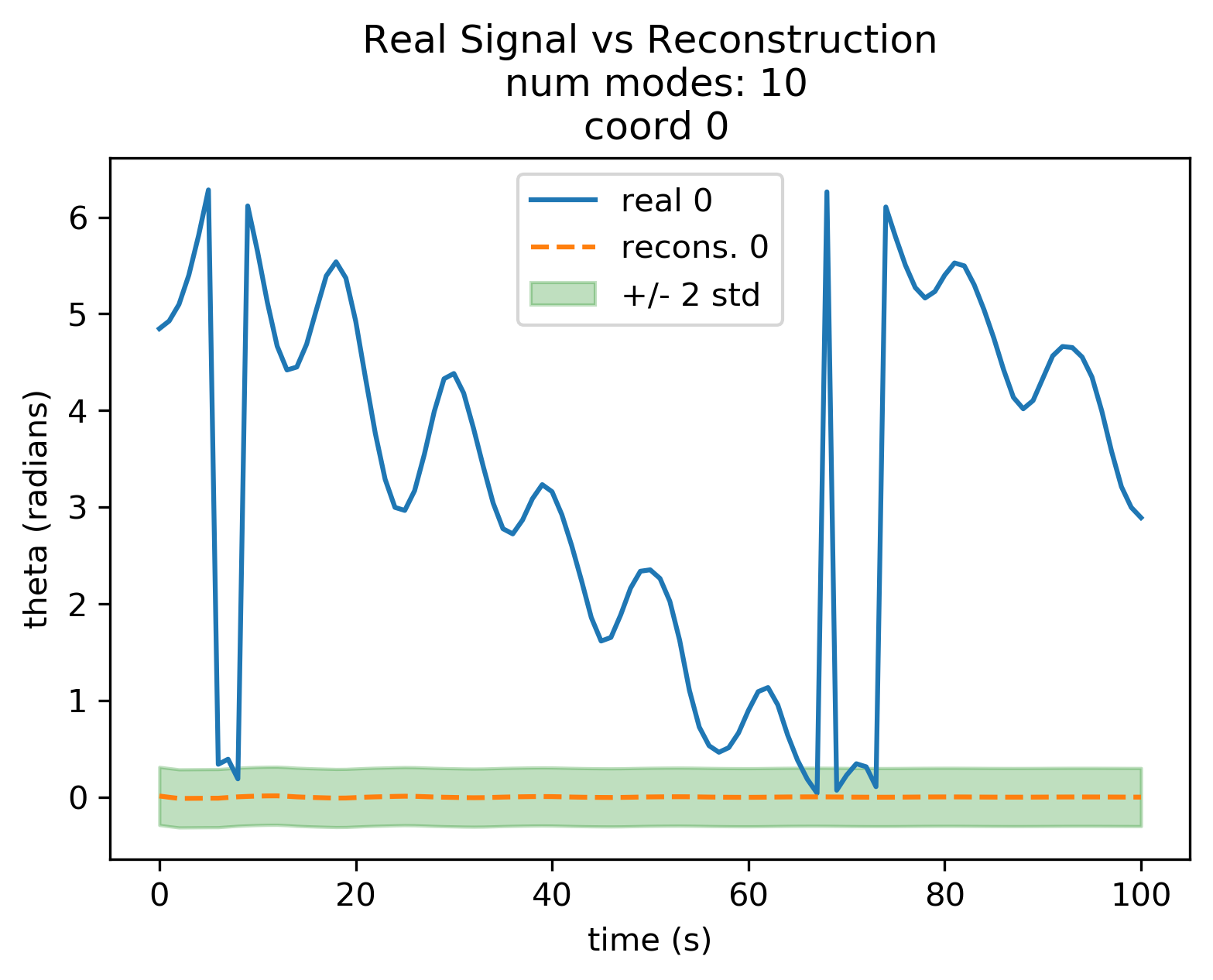
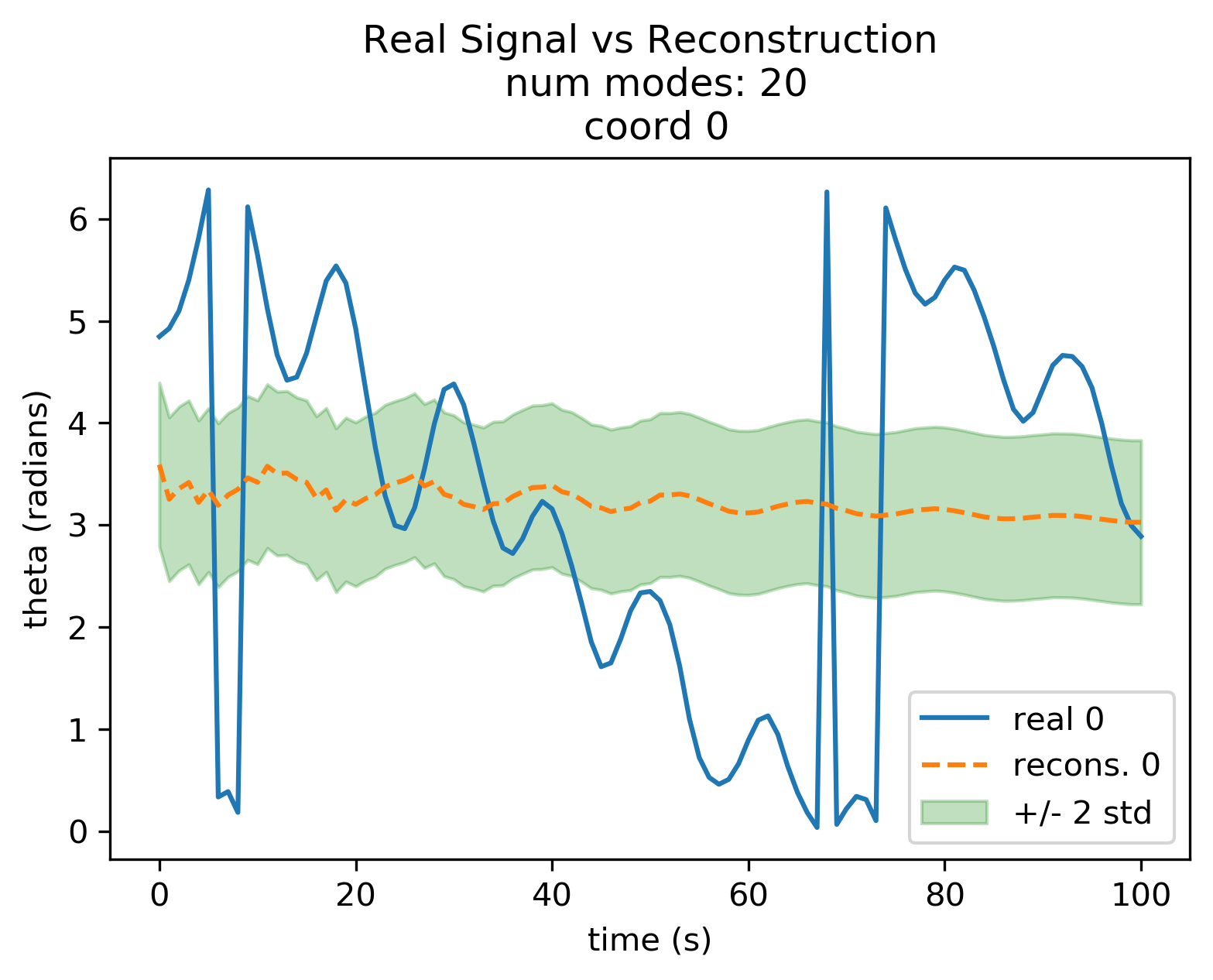
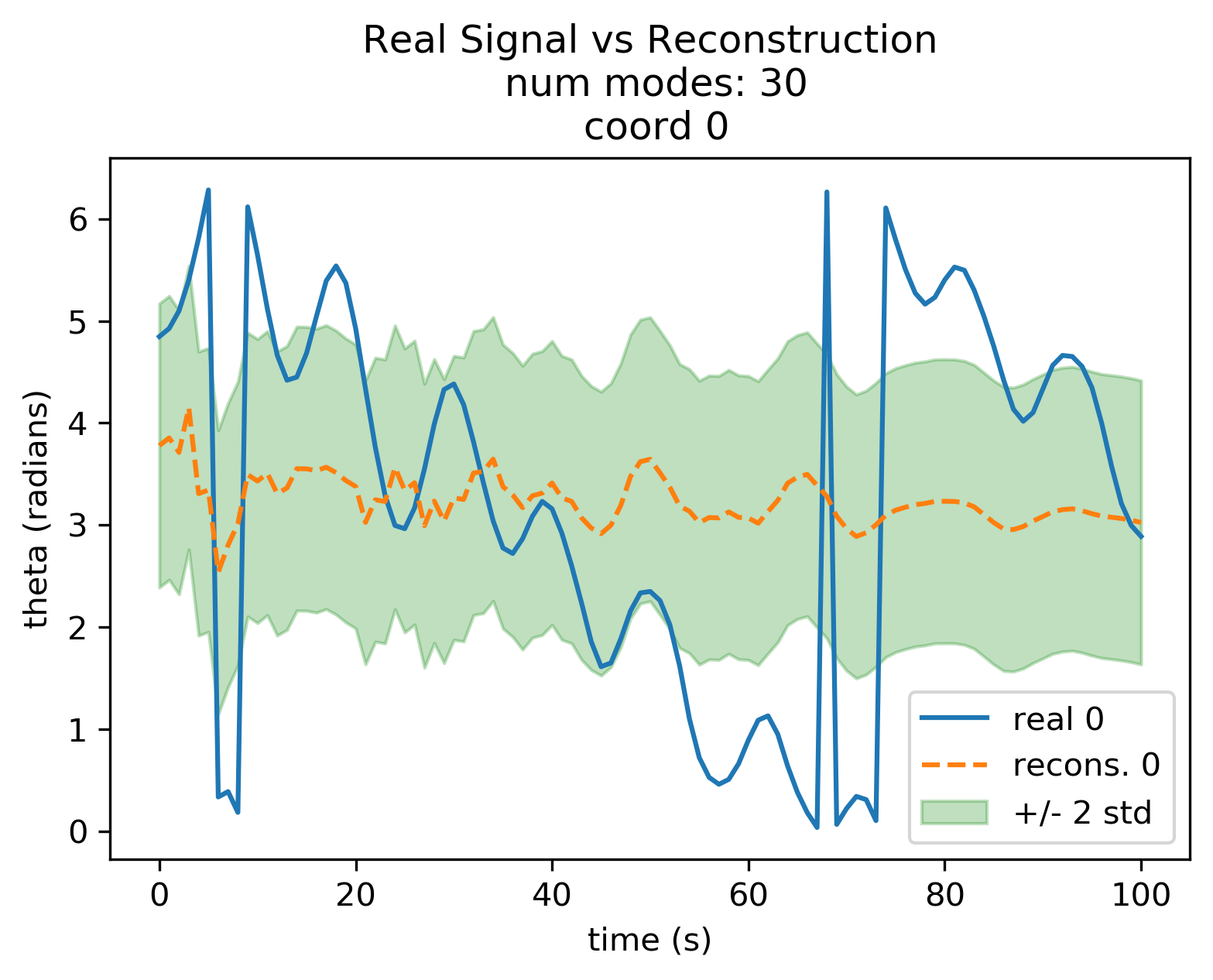
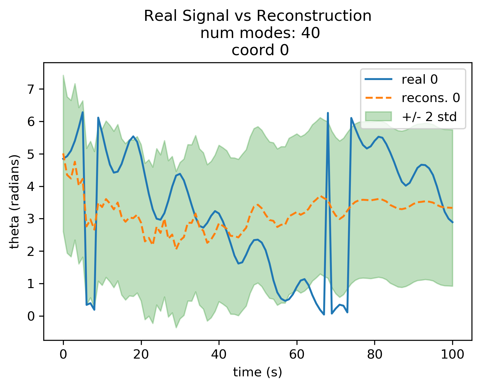
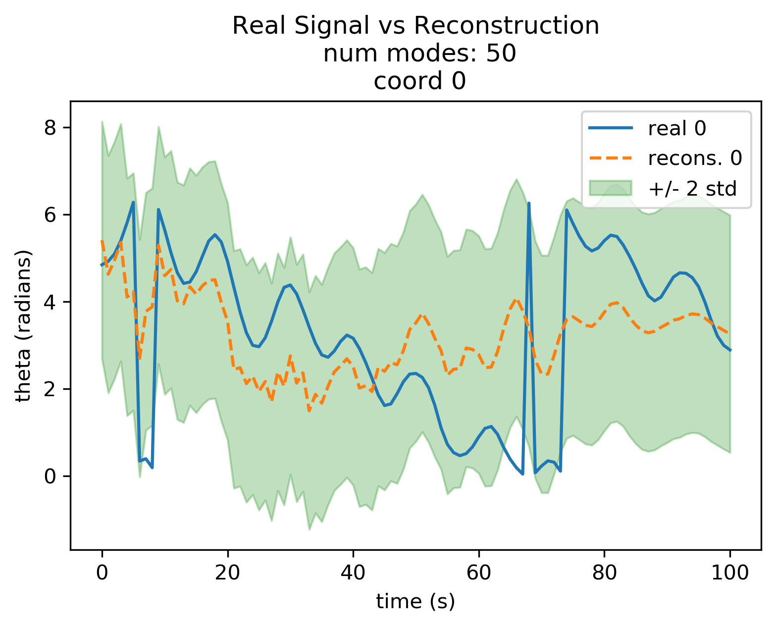
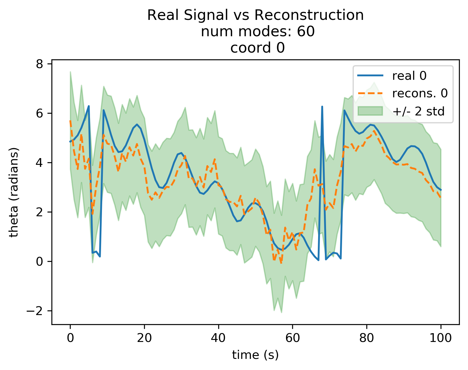
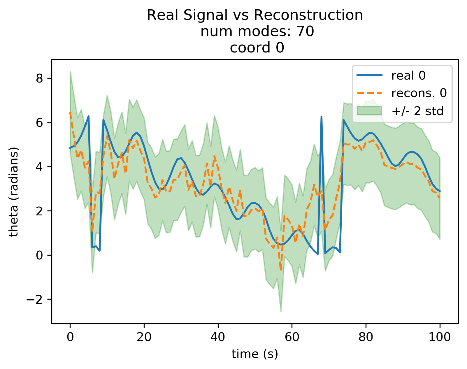
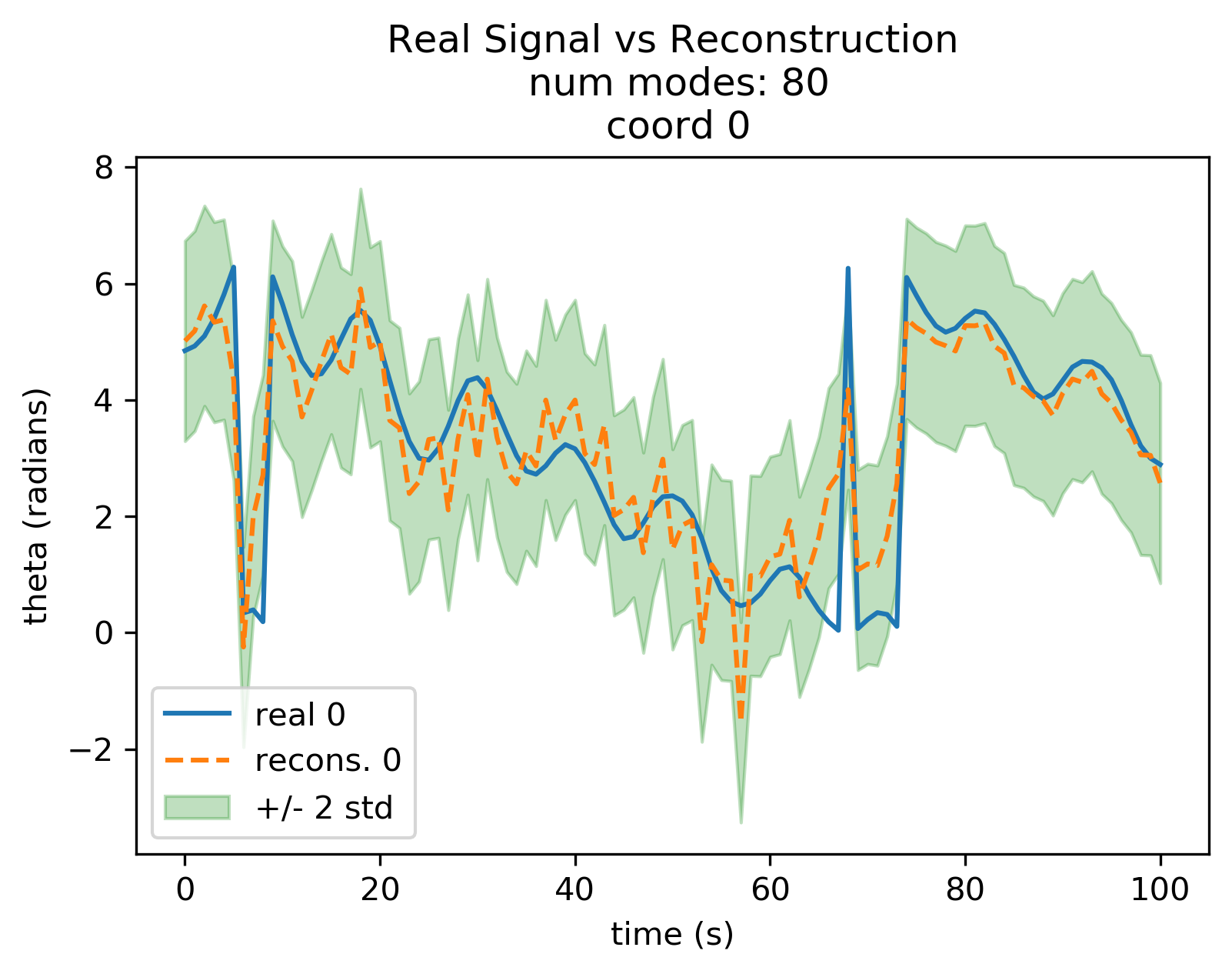
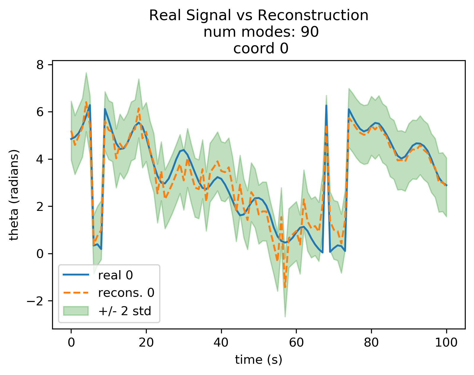
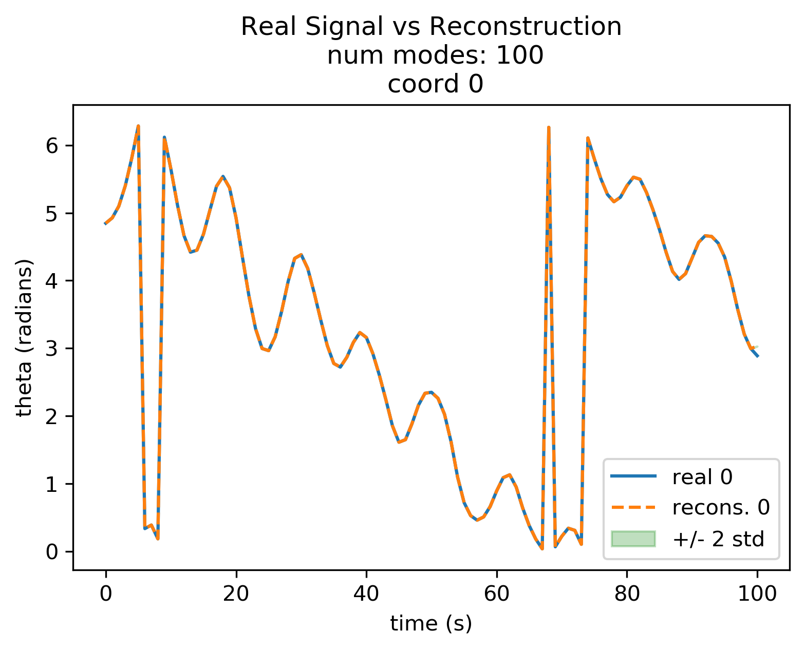
Figure 22: Type 1 Kuramoto models, signal vs reconstruction: Comparison of the true signal with reconstruction signals using $10,20,30,\dots,100$ modes for reconstruction for oscillator 0. The true signal is in blue. The reconstruction signal is orange and the green band is $\pm 2$ standard deviations of the modal noise.

Figure 23: Type 2 Kuramoto models, signal vs reconstruction: Comparison of the true signal with reconstruction signals using $10,20,30,\dots,100$ modes for reconstruction for oscillator 0. The true signal is in blue. The reconstruction signal is orange and the green band is $\pm 2$ standard deviations of the modal noise.

References

- [1] J. A. Acebrón, L. L. Bonilla, C. J. P. Vicente, F. Ritort, and R. Spigler, The kuramoto model: A simple paradigm for synchronization phenomena, Reviews of modern physics, 77 (2005), p. 137.
- [2] S. Bagheri, Effects of weak noise on oscillating flows: Linking quality factor, floquet modes, and koopman spectrum, Physics of Fluids, 26 (2014), p. 094104.
- [3] S. L. Brunton, J. L. Proctor, and J. N. Kutz, Discovering governing equations from data by sparse identification of nonlinear dynamical systems, Proceedings of the national academy of sciences, 113 (2016), pp. 3932–3937.
- [4] M. Budišić, R. Mohr, and I. Mezić, Applied koopmanism, Chaos: An Interdisciplinary Journal of Nonlinear Science, 22 (2012), p. 047510.
- [5] S. T. Dawson, M. S. Hemati, M. O. Williams, and C. W. Rowley, Characterizing and correcting for the effect of sensor noise in the dynamic mode decomposition, Experiments in Fluids, 57 (2016), p. 42.
- [6] Z. Drmac, I. Mezic, and R. Mohr, Data driven modal decompositions: analysis and enhancements, SIAM Journal on Scientific Computing, 40 (2018), pp. A2253–A2285.
- [7] Z. Drmac, I. Mezic, and R. Mohr, Data driven koopman spectral analysis in vandermonde–cauchy form via the dft: Numerical method and theoretical insights, SIAM Journal on Scientific Computing, 41 (2019), pp. A3118–A3151.
- [8] Z. Drmac, I. Mezic, and R. Mohr, On least squares problems with certain vandermonde–khatri–rao structure with applications to dmd, SIAM Journal on Scientific Computing, 42 (2020), pp. A3250–A3284.
- [9] N. Galioto and A. A. Gorodetsky, Bayesian system id: optimal management of parameter, model, and measurement uncertainty, Nonlinear Dynamics, 102 (2020), pp. 241–267.
- [10] A. R. Gerlach, A. Leonard, J. Rogers, and C. Rackauckas, The koopman expectation: an operator theoretic method for efficient analysis and optimization of uncertain hybrid dynamical systems, arXiv preprint arXiv:2008.08737, (2020).
- [11] M. S. Hemati, C. W. Rowley, E. A. Deem, and L. N. Cattafesta, De-biasing the dynamic mode decomposition for applied koopman spectral analysis of noisy datasets, Theoretical and Computational Fluid Dynamics, 31 (2017), pp. 349–368.
- [12] B. O. Koopman, Hamiltonian systems and transformation in Hilbert space, Proceedings of the National Academy of Sciences of the United States of America, 17 (1931), p. 315.
- [13] A. Lasota and M. C. Mackey, Chaos, fractals, and noise: stochastic aspects of dynamics, vol. 97, Springer, 1994.
- [14] Y. Lian and C. N. Jones, On gaussian process based koopman operators, IFAC-PapersOnLine, 53 (2020), pp. 449–455.
- [15] I. Mezić, Spectral properties of dynamical systems, model reduction and decompositions, Nonlinear Dynamics, 41 (2005), pp. 309–325.
- [16] I. Mezić, Spectrum of the koopman operator, spectral expansions in functional spaces, and state-space geometry, Journal of Nonlinear Science, 30 (2020), pp. 2091–2145.
- [17] I. Mezić and A. Banaszuk, Comparison of systems with complex behavior, Physica D: Nonlinear Phenomena, 197 (2004), pp. 101–133.
- [18] C. W. Rowley, I. Mezić, S. Bagheri, P. Schlatter, and D. S. Henningson, Spectral analysis of nonlinear flows, Journal of Fluid Mechanics, 641 (2009), pp. 115–127.
- [19] P. J. Schmid, Dynamic mode decomposition of numerical and experimental data, Journal of Fluid Mechanics, 656 (2010), pp. 5–28.
- [20] R. K. Singh and J. S. Manhas, Composition operators on function spaces, vol. 179, Elsevier, 1993.
- [21] J. H. Tu, Dynamic mode decomposition: Theory and applications, PhD thesis, Princeton University, 2013.
- [22] M. Wanner and I. Mezic, Robust approximation of the stochastic koopman operator, SIAM Journal on Applied Dynamical Systems, 21 (2022), pp. 1930–1951.
- [23] M. O. Williams, I. G. Kevrekidis, and C. W. Rowley, A data–driven approximation of the koopman operator: Extending dynamic mode decomposition, Journal of Nonlinear Science, 25 (2015), pp. 1307–1346.