CyRSoXS: A GPU-accelerated virtual instrument for Polarized Resonant Soft X-ray Scattering (P-RSoXS)

Abstract

Polarized Resonant Soft X-ray scattering (P-RSoXS) has emerged as a powerful synchrotron-based tool that combines principles of X-ray scattering and X-ray spectroscopy. P-RSoXS provides unique sensitivity to molecular orientation and chemical heterogeneity in soft materials such as polymers and biomaterials. Quantitative extraction of orientation information from P-RSoXS pattern data is challenging because the scattering processes originate from sample properties that must be represented as energy-dependent three-dimensional tensors with heterogeneities at nanometer to sub-nanometer length scales. We overcome this challenge by developing an open-source virtual instrument that uses Graphical Processing Units (GPUs) to simulate P-RSoXS patterns from real-space material representations with nanoscale resolution. Our computational framework – called CyRSoXS (https://github.com/usnistgov/cyrsoxs) – is designed to maximize GPU performance, including algorithms that minimize both communication and memory footprints. We demonstrate the accuracy and robustness of our approach by validating against an extensive set of test cases, which include both analytical solutions and numerical comparisons, demonstrating a speedup of over three orders relative to the current state-of-the-art P-RSoXS simulation software. Such fast simulations open up a variety of applications that were previously computationally infeasible, including (a) pattern fitting, (b) co-simulation with the physical instrument for operando analytics, data exploration, and decision support, (c) data creation and integration into machine learning workflows, and (d) utilization in multi-modal data assimilation approaches. Finally, we abstract away the complexity of the computational framework from the end-user by exposing CyRSoXS to Python using Pybind. This eliminates input/output (I/O) requirements for large-scale parameter exploration and inverse design, and democratizes usage by enabling seamless integration with a Python ecosystem (https://github.com/usnistgov/nrss) that can include parametric morphology generation, simulation result reduction, comparison to experiment, and data fitting approaches.

tcb@breakable nist]Material Measurement Laboratory, National Institute of Standards and Technology (NIST), Gaithersburg, MD 20899, USA nist]Material Measurement Laboratory, National Institute of Standards and Technology (NIST), Gaithersburg, MD 20899, USA ucsb]Materials Department, University of California, Santa Barbara, CA 93106, USA. nist]Material Measurement Laboratory, National Institute of Standards and Technology (NIST), Gaithersburg, MD 20899, USA nist]Material Measurement Laboratory, National Institute of Standards and Technology (NIST), Gaithersburg, MD 20899, USA nist]Material Measurement Laboratory, National Institute of Standards and Technology (NIST), Gaithersburg, MD 20899, USA nist]NIST Center for Neutron Research, National Institute of Standards and Technology (NIST), Gaithersburg, MD 20899, USA ucsb]Materials Department, University of California, Santa Barbara, CA 93106, USA. nist]Material Measurement Laboratory, National Institute of Standards and Technology (NIST), Gaithersburg, MD 20899, USA

1 Introduction

Developing process-structure-property relationships is a central pillar of material science and engineering research. Understanding the effect of composition, structure, and processing on the performance of a material can enable the intelligent and efficient tuning of the process variables to improve the end performance of the material in a given application. With these process-structure-property relationships, the exciting goal of designing new materials instead of discovering them becomes a reality. Thus, there is an ever-present need to develop new characterization methods to elucidate material structure with increasing detail and clarity.

Structural characterization is particularly challenging in soft matter due to its semi-disordered nature. Some important aspects of soft material structure include spatial heterogeneities in composition, density, molecular orientation/conformation, and the degree of order. Recent advancements in synthesis and materials processing have unlocked access to systems in which all aspects of soft material structure might ultimately be controlled by design. However, despite an enormous acceleration in the capability and speed of characterization methods across many length scales, it remains a fundamental and pervasive challenge to efficiently, rigorously, and robustly assimilate materials structure characterization data streams into a self-consistent digital twin that describes material structure. If achieved, the resultant comprehensive structural description would allow us to understand, predict, and eventually control how material properties arise from a complex interplay of different aspects of structure across relevant length scales.

In this context, there have been recent efforts to integrate computational tools with experimental data streams. Virtual instruments that mimic the physical principles of the characterization method—X-ray diffraction, light spectroscopy, electron transmission ¹, ², ³, ⁴—can transform how downstream analysis of experimental data streams is performed. For instance, a virtual instrument can enable rapid data quality evaluation and provide statistically rigorous estimates of when enough data has been collected. Such approaches can maximize the utilization of heavily-subscribed instruments at centralized facilities such as X-ray and neutron sources. Furthermore, a virtual instrument can allow principled down-selection of plausible hypotheses for developing structure-property relationships. Such virtual tools also allow formal analysis and characterization of uncertainty, identify the most sensitive features, and allow in silico experimentation before performing physical experiments for greater efficiency in experiment execution. Finally, the success of artificial intelligence and machine learning (AI/ML) methods ⁵, ⁶, ⁷, ⁸ point to the possibility of integrating experimental data with the virtual instrument to provide automated and formal approaches to assimilating complementary data streams—for instance, real space (electron microscopy) and frequency space (X-ray diffraction)—to create a self-consistent and multimodal digital twin.

Polarized Resonant Soft X-ray scattering (P-RSoXS) is a recently developed technique with unique characterization abilities ⁹ and an excellent candidate for developing a virtual instrument. Typical scattering experiments performed at hard X-ray energies provide a very low contrast between organic constituents in a material. P-RSoXS  overcomes this limitation by combining conventional small-angle X-ray scattering (SAXS) with soft X-ray spectroscopy to yield a tunable scattering contrast. The energies of this soft X-ray are scanned across absorption edges of the light elements (C, N, O), commonly found in organic materials, often yielding significant contrast variation and substantially improved signal-to-noise ratio for organic systems. P-RSoXS  thus provides a path to probe the structure in the $\mathrm{nm-\mu m}$ range with both chemical and physical sensitivity without the need to perturb the system with labels such as the heavy element ”stains” commonly used to enhance SAXS or the radioisotopes commonly used to enhance small angle neutron scattering (SANS). The contrast enhancement makes P-RSoXS particularly useful for probing the structure of thin ($<$ 200 nm) films, samples that are challenging for hard X-rays and neutrons due to the small scattering volumes. Composition contrast with P-RSoXS is so significant that short exposures of thin films – less than 1 min at normal incidence – at resonant energies with high contrast will yield patterns with quality similar to conventional bulk SANS patterns requiring mm-scale sample volumes and hours to collect. The approach also does not require grazing-incidence geometries which are commonly used to gain signal in the X-ray scattering of thin films.

The variable sensitivity of P-RSoXS to each chemical bond can amplify scattering intensity even with only small chemical differences between materials, which enables the extraction of useful structure information for heterogeneous materials. A unique aspect of P-RSoXS  is that it is sensitive to molecular orientation via interaction of the soft X-ray electric field vector with oriented transition dipoles within the sample. Complex P-RSoXS  patterns can arise from orientational heterogeneities. This unique aspect of P-RSoXS  provides exciting opportunities for characterizing previously unmeasurable aspects of the structure of soft materials, but it makes adapting conventional SAXS or SANS analysis approaches nearly impossible because the materials properties that affect contrast in those techniques are effectively scalar quantities. A new analysis framework is required to represent independent fluctuations in material composition and molecular orientation on sub-nanometer length scales. The availability of a virtual analog to P-RSoXS  will enable the discovery and quantification of structure in complex, chemically heterogeneous soft systems. Motivated by this exciting promise, here we will describe our development of CyRSoXS – a fast, graphics processing unit (GPU) accelerated virtual instrument for Polarized Resonant Soft X-ray scattering (P-RSoXS).

To dispel any question regarding which technique we address herein, we note that, because P-RSoXS  is not yet a mainstream technique, a variety of different acronyms have been proposed for it, including ”R-SoXS” and ”PAXS.”¹⁰ The community now appears to have settled on ”RSoXS” and ”P-RSoXS.” It is not uncommon for practitioners to use only ”RSoXS” when exploiting its composition contrast capabilities and to use ”P-RSoXS” when adding its orientation contrast capabilities. We should mention, however, that these contrast modes are intrinsically linked. It is not possible to perform RSoXS without polarization and its concomitant molecular orientation sensitivity. Even circular polarization will yield patterns that can be significantly affected by molecular orientation effects. These principles suggest that model-free, composition-only analyses of P-RSoXS in systems having significant but ignored molecular orientation fluctuations may yield incorrect results, a situation that could be greatly improved with a fast virtual instrument.

Current state-of-art: The current state-of-the-art P-RSoXS simulator, developed by Gann et al. ¹⁰ in Igor Pro has been pivotal in answering many scientific questions ¹¹, ¹², ¹³, ¹⁴, ¹⁵, ¹⁶. However, it has limitations on practical deployment in terms of speed and no opportunity for deployment on the state-of-the-art high performance computing (HPC) clusters. These limitations become most apparent when attempting to fit experimental data using goal-seeking algorithms that adjust material structure input parameters to obtain agreement between simulation and experiment. Such optimization routines require a significant number of forward simulations and thereby motivate the need for the fast forward simulator. The commercial licensing of Igor Pro further hinders the democratization and availability of the tool to many researchers. There has been rapid growth in the interest in leveraging advances in Machine Learning and Data Analytics among material scientists for material design and exploration. The availability of a fast forward simulator is a critical necessity for data creation and integration into Machine Learning Model Operationalization (MLOps) workflows. More practically, since Python has become the de-facto language for data analysis and Machine Learning, the currently available simulator does not provide any straightforward integration for researchers to utilize such tools.

Our contributions: We build upon an earlier framework that modeled the physics of soft X-ray scattering through a heterogeneous thin film ¹⁰. In particular, we significantly speed up execution time and, via integration with a Python ecosystem, incorporate substantial additional functionality. Our key contributions in this paper are:

• Accomplish near real-time simulation of RSoXS at sizes/resolutions (up to $2^{28}$ or 268 million voxels) that were hitherto not possible.

• Use GPU acceleration to achieve 1000 $\times$ speedup over current state-of-art approaches. This is achieved by careful design of “GPU-friendly” data structure and algorithms— including memory and communication considerations.

• Careful software design of a simulation engine that lies at the center of a feature-rich data analysis and model exploration ecosystem when combined with Python code bases for morphology generation, simulation result reduction, and data-fitting. Python binding democratizes access, simplifies usage, and enables seamless integration with AI / ML libraries and eliminates the bottleneck of I/O operation, especially during parameter exploration or inverse design.

• A new and well-documented voxel-based material structure data file format in Hierarchical Data Format-5 (HDF5) that includes capabilities for verbose metadata, multiple materials, independent representation of composition and orientation, and an intuitive Euler angle description of material orientation.

• An extensive set of validation examples developed by a growing community across multiple institutions.

• Tutorials that serve as unit tests for this open-source framework. The full software stack is open-source and requires access to CUDA-enabled hardware.

The rest of the paper is organized as follows: We begin by briefly introducing P-RSoXS in Section 2, followed by a detailed mathematical model in Section 3; We detail the data structures and algorithms in Section 4, and present results including validation cases in Section 5. We show the performance of CyRSoXS with varying problem size and scaling to multiple GPUs in Section 6. We discuss integration with Python environments in Section 7, and we conclude by discussing the implications and path for future developments in Section 8.

2 Polarized Resonant Soft X-ray Scattering (P-RSoXS)

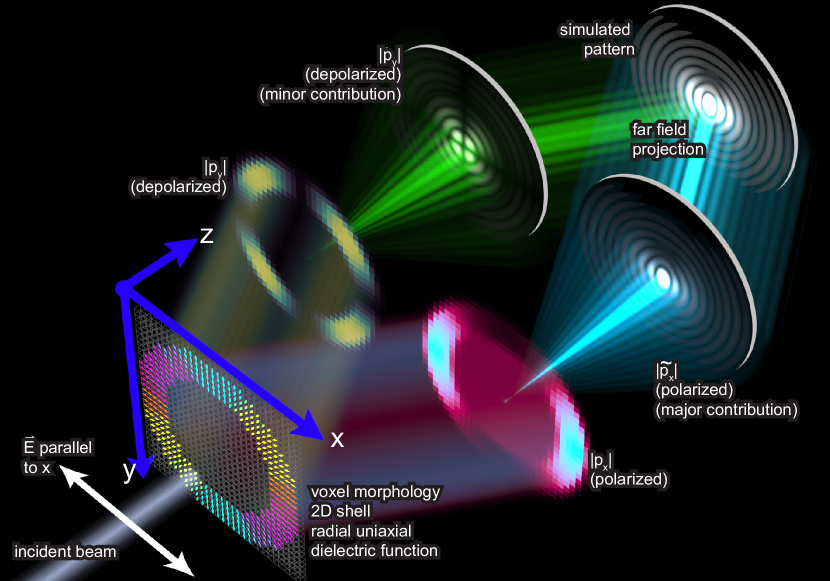
Figure 1: Schematic of P-RSoXS, where a polarized soft X-ray beam passes through a sample, interacting with and scattering off the electrons in that sample; these scattered X-rays are collected on an X-ray sensitive detector.

In P-RSoXS, a polarized soft X-ray beam passes through a sample, interacting with and scattering off the electrons in that sample; these scattered X-rays are collected on an X-ray sensitive detector (typically charge coupled device (CCD) or complementary metal oxide semiconductor (CMOS)). Fig. 1 shows a condensed version of the physical principles of P-RSoXS, which are explained in greater detail in a recent comprehensive review of the technique and its application to soft materials.⁹ This photon-electron interaction strength depends on the X-ray energy and the chemistry of the molecules within the sample. At energies far from an absorption edge, X-rays interact equally with all electrons in the sample, and the interaction strength scales directly with the electron density. Near an absorption edge, the interaction strength increases dramatically when the incident X-ray energy is commensurate with the energy required to resonantly excite an electron to an unoccupied molecular orbital. The K-absorption edge of many lightweight elements (C, O, N, F) lies in the soft X-ray energy regime ($100$ $eV\lesssim E_{photon}\lesssim~{}2$ $keV$); all are commonly exploited in P-RSoXS. Selection of the incident energy near the core binding energy of the electrons makes the technique element-specific, whereas the chemical bonds that define the excited state unoccupied molecular orbital energy make the technique sensitive to specific bonds or moieties. The spectroscopic scattering pattern thus provides a tunable, chemically-sensitive probe of nanoscale and mesoscale components in a heterogeneous complex material ¹⁷.

The resonant soft X-ray absorption is described by a transition dipole moment that couples the initial and final states. The initial state of the electron is a core orbital that is spherically symmetric, therefore the geometric dependence of the interaction strength is defined by the unoccupied molecular orbital, which for most soft X-ray resonances can be represented as vectors or planes parallel or perpendicular to the bond ¹⁸. Soft X-ray absorption, a principal contributor to scattering contrast, varies as the dot product of the electric field vector and the transition dipole moment. This interaction makes P-RSoXS  sensitive to spatial distributions in molecular orientation. For instance, in the case of carbon fused ring compounds, when the X-ray energy is in resonance with the fundamental carbon electron transition (C1$s\xrightarrow{}\pi^{*}$), the molecules exhibit vector transition dipole moments perpendicular to the ring planes ¹⁹. Two identical molecules oriented differently within a sample will have different interaction strengths with a fixed electric field vector, and there will be a scattering contrast between them. If the orientation of these molecules is spatially correlated in a sample, a scattering pattern will be observed. For example, P-RSoXS can detect correlated interfacial molecular orientation regions (such as mixtures of amorphous, semi-crystalline, or liquid crystalline phases). Crystalline, semi-crystalline, and liquid-crystalline organic materials have locally large anisotropic bond orientation statistics, impacting the mechanical, optical, and electronic properties of these materials. Understanding these relative orientations at different length scales is necessary for a detailed understanding of organic thin-film devices. In addition, P-RSoXS had been shown to reveal local molecular alignment independent of overall crystallinity and represents an essential new tool for understanding the structure-property relationship and examining the connection between transport properties and morphology in organic and hybrid organic-inorganic electronic devices.

The interaction of X-rays with a system can be encoded using a 3D analog of the complex index of refraction, $\underline{\underline{\mathbf{N}}}$. Each component of this tensor is a function of the dispersive and absorptive components of the index of refraction, $N_{ij}(E)=f(\delta(E),\beta(E))$, where E is the photon energy, $\delta$ is the dispersive component, and $\beta$ is the absorptive component of the index of refraction. In the hard X-ray regime, far away from the resonance frequency of the constituent atoms, the real part of the complex index of refraction is a scalar proportional to the electron density of the material. The imaginary part is negligible due to low absorption, and the electron density difference between constituent materials determines the scattering contrast of the system. However, close to the absorption edge of the constituent atoms, the electrons get excited to the unoccupied molecular states or vacuum, and therefore $\beta$ will naturally exhibit peaks and other absorption features that will differ depending on orientation; changes in $\delta$ are also expected due to causality and can be calculated using the Kramers-Kronig relations ^{20, 21}.

3 Mathematical Model

Notation

Having described the overall mechanism of P-RSoXS, we next detail the mathematics of the simulation.

3.1 Morphology:

Consider a morphology composed of a $c$ component mixture. We discretize the morphology into a uniformly spaced voxel grid. Each voxel contains some (or all) of the $c$ components. Each of these components can either be amorphous or can be oriented. If a component is oriented, we assume that it is well represented by a uniaxial representation. 

A key advantage of the uniaxial assumption is that it is simple and allows the construction of a simple, abstract model of properties within a voxel. This abstract model and associated data structures are independent of the material and energy. The abstract model can then be combined with a material library, which can be stored in memory, to allow the same model to be re-used for different materials and different energies. This abstract representation requires only two scalar fractions (volume fraction and orientation fraction) and two Euler angles per material/voxel for the uniaxial assumption. In contrast, a biaxial representation would require five scalar fractions (volume fraction and four orientation mixing parameters) with three Euler angles for a similar abstract model. To represent arbitrary distributions of a biaxial representation in an abstract model would require including non-diagonal elements of the full tensor for 19 unique scalar fractions (volume fraction, six elements with 3 coefficients each on the original ”molecular” biaxial elements), significantly increasing memory and communication footprints.

A uniaxial representation conveys the necessary properties for materials with a single dominant orientation mode of one particular molecular axis, which we judge to be a large number of use cases. If a more faithful representation of a multimodal orientation distribution is required, that can be approached in our framework using by breaking a component into additional materials with identical dielectric functions and volume fractions that add to the total for that component, but which have distinct orientations reflecting the expected distribution. If a more faithful representation of molecular-level properties is required, it is possible to use a system of uniaxial functions to represent an underlying biaxial function, but that is not a currently supported use case for our approach. We will lay out a clear pathway to relax this assumption and consider biaxial representation in the next release version of CyRSoXS.

Each voxel, therefore, has four features associated with each component $j=1\dots c$:

• $v_{frac}^{j}$: fraction of volume occupied by component $j$ in this voxel. By definition, 0 $\leq$ $v_{frac}^{j}$ $\leq$ 1, and the sum $v_{frac}^{j}$ across all $j$ (that is, the sum of all volume fractions of all materials) within a voxel is expected to be 1.0, CyRSoXS will not check whether they sum to one, although such checking can be done with model visualization code provided in our broader Python ecosystem. We encourage as a best practice the use of vacuum as an explicit material in the model, such that model self-consistency is straightforward to confirm.

• $s^{j}$: degree of alignment of component $j$ in this voxel. This parameter indicates the volume fraction of component $j$ that is oriented (as opposed to unaligned). We expect that 0 $\leq$ $s^{j}$ $\leq$ 1, but unlike $v_{frac}^{j}$, there is no expectation of any constraint involving other materials. $s^{j}$ is a relative volume fraction; in other words $s^{j}$ is multiplied by $v_{frac}^{j}$ to yield the absolute volume fraction of oriented material j in a voxel (see Eq. 2 below). This parameter is conceptually identical to the well-known uniaxial ”orientational order parameter,” $S$, but only in the range of 0 $\leq$ $S$ $\leq$ 1, where $S$ = 1 indicates complete alignment with a director (our director is defined by the Euler angles described below) and $S$ = 0 indicates an isotropic condition. We note that the orientational order parameter $S$ can also include the range -0.5 $\leq$ $S$ $\leq$ 0, which indicates orientation perpendicular to the director, but we do not support values of $s^{j}$ less than zero. Expressing perpendicular orientations should instead be accomplished by explicit adjustment of Euler angles.

• $\phi^{j}$: orientation feature 1, defined as the (first) rotation of component $j$ about the Z-axis.

• $\theta^{j}$: orientation feature 2, defined as (second) rotation of component $j$ about the (original) Y-axis.

The last two features represent the Euler angle representation of material orientation in a voxel.

We refrain from providing overly prescriptive guidance on model design because there may be use cases for CyRSoXS that we cannot anticipate. However, we offer here some model design choices that have worked well for our internal testing and for many of our validation cases provided in Section 5. Most models will represent the real-space structure of a thin film, so they will typically have larger $x$ and $y$ ”lateral” dimensions and a smaller $z$ ”height” dimension. We consider it a best practice for $x$ and $y$ to have the same dimensions and resolutions. Common $x$ and $y$ dimensions (meaning the length of the whole model on a lateral side) are micron scale, perhaps ranging from (0.5 to 5) $\mu$m. Common lateral resolutions include 512 $\times$ 512, 1024 $\times$ 1024, and 2048 $\times$ 2048, although larger sizes are possible. The $z$ resolution is usually a smaller multiple of 2; common values include 32, 64, and 128. The voxels are considered perfect cubes in CyRSoXS, such that the model dimensions are the product of the resolution and the length of a voxel side. These model dimensions and resolutions correspond to voxels with side lengths in the (0.2 to 10) nm range.

These model dimensions and resolutions are compatible with data fusion workflows where real-space images derived from atomic force microscopy (AFM), transmission electron microscopy (TEM), or other imaging methods are used as a foundation for CyRSoXS model creation. In some cases such images could be used to assign $v_{frac}^{j}$ across voxels for different components, depending on the contrast mode of the imaging. The other voxel-level parameters, $s^{j}$, $\phi^{j}$, and $\theta^{j}$ will most likely not be available from imaging methods because there is a lack of techniques that are sensitive to molecular orientation in soft materials at the nanoscale. (This fact provides much of our motivation for investment in P-RSoXS  interpretation!) Hypothesis driven parametric assignment of $s^{j}$, $\phi^{j}$, and $\theta^{j}$ might instead be employed. Models built entirely parametrically are certainly possible, as demonstrated for many of our validation cases shown in Section 5.

A brief primer on Euler angles: For Euler angles, we use the ZYZ convention. We assume that the primary alignment axis starts parallel to Z - axis (0,0,1) (Fig. 2(a)). This is also the default direction of the simulated incident beam. According to this convention (Fig. 2), and with reference to the rotation matrices B, C, and D, which are further defined in Equation (3):

1. The first rotation is by an angle $\varphi$ about the Z-axis using rotation matrix D. (Fig. 2(b))

2. The second rotation is by an angle $\theta$ about the original Y-axis using rotation matrix C.(Fig. 2(c))

3. The third rotation is by an angle $\psi$ about the original Z-axis using rotation matrix B.(Fig. 2(d))

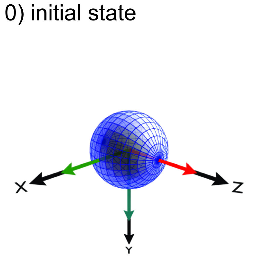
(a) Initial state

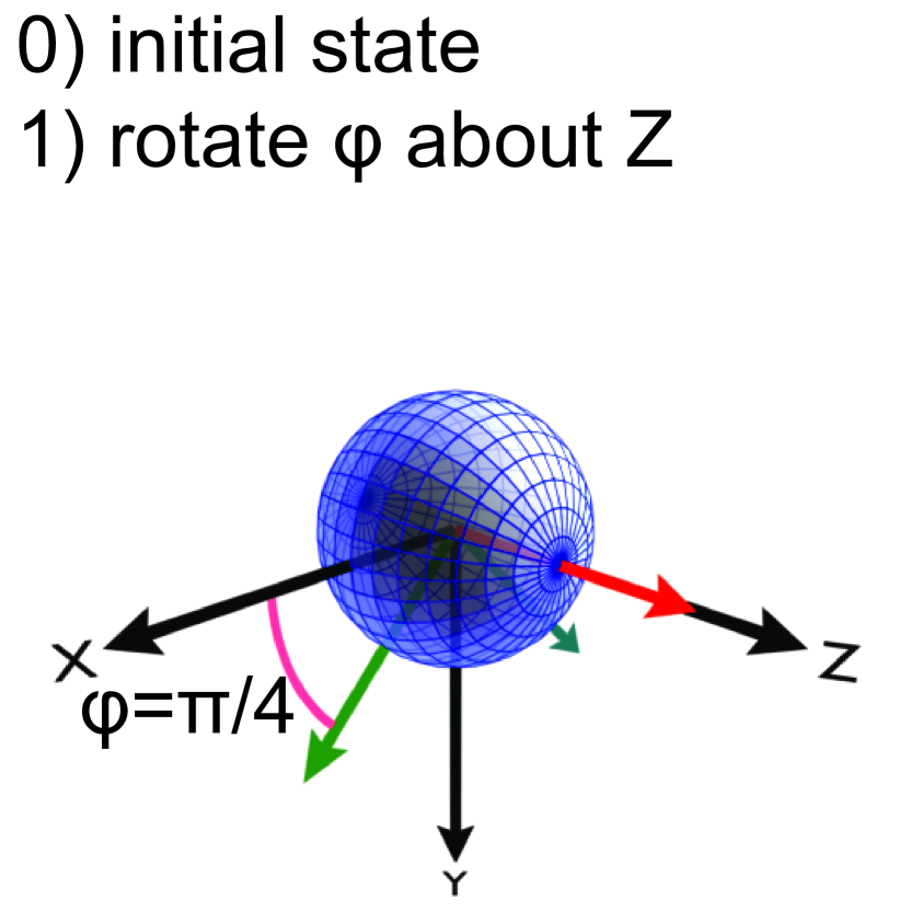
(b) $\phi$ around Z

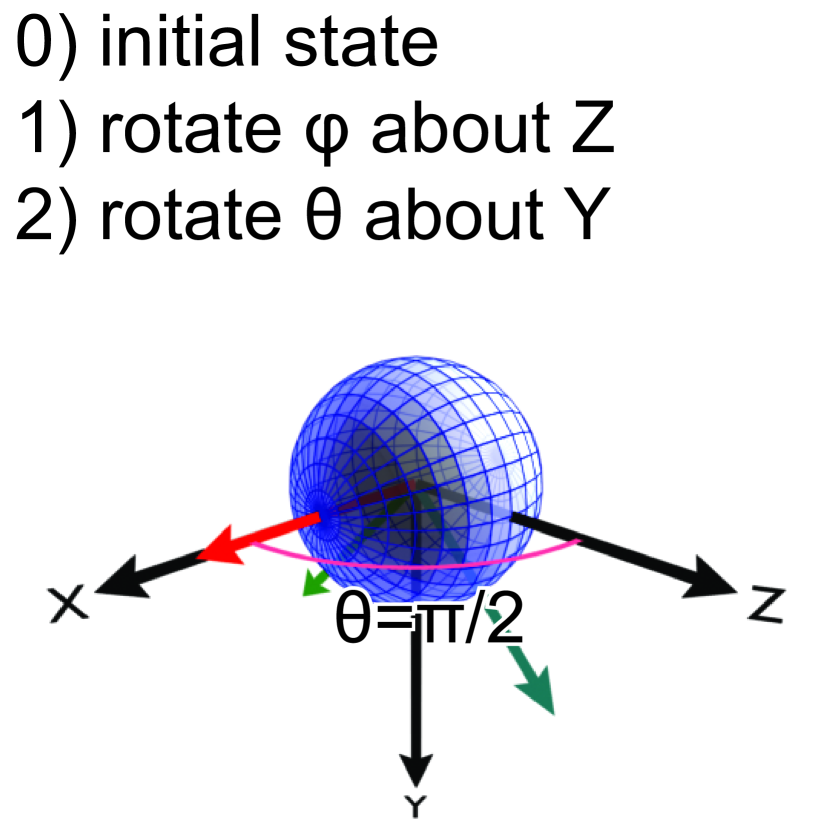
(c) $\theta$ around Y

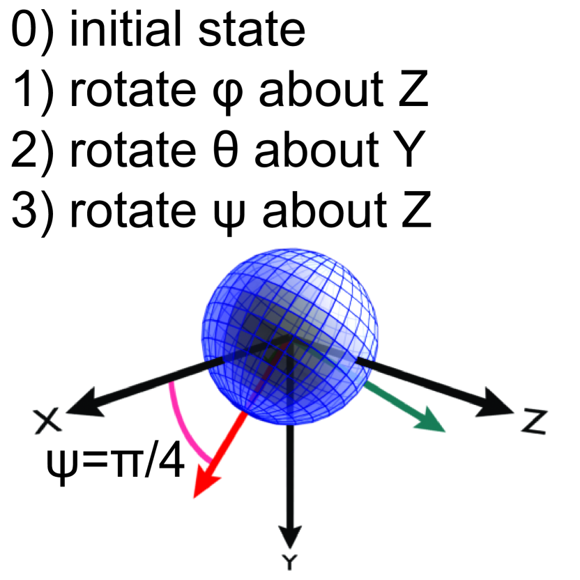
(d) $\psi$ around Z

Figure 2: Different steps of the Euler angle rotation.

We note that other conventions are possible and have been used in the literature; for instance,  Gann et al. ¹⁰ used the vector orientation in 3D space to define an equivalent morphology. These equivalent conventions can be easily transformed into the Euler angles using suitable rotation transformations. A benefit of our convention is its straightforward expandability into a biaxial representation by adding a third Euler angle.

3.2 Material properties:

As mentioned in Section 2, the interaction of soft X-rays with a material is encoded in the 3D analog, $\underline{\underline{\mathbf{N}}}$, of the material-specific, complex index of refraction. $\underline{\underline{\mathbf{N}}}$ is a $3\times 3$ data structure that exhibits energy dependence. For a uniaxial system, $\underline{\underline{\mathbf{N}}}$ can be diagonalized as:

$$\underline{\underline{\mathbf{N}}}=\begin{pmatrix}n_{\parallel}&0&0\\ 0&n_{\bot}&0\\ 0&0&n_{\bot}\end{pmatrix}$$ (1)

We will refer to $\underline{\underline{\mathbf{N}}}$ as the refractive index for brevity, with the understanding that it actually is a convenient 3D analog to the complex index of refraction.

3.3 Mathematical representation of P-RSoXS

The mathematical operations that mimic P-RSoXS can be divided into 6 steps:

1. Effective Refractive Index: For each voxel, the effective refraction tensor for material component $j$ can be computed using the aligned and unaligned fraction as:

   $$\footnotesize\underline{\underline{\mathbf{N_{eff}}}}^{j}=v^{j}_{frac}\bigg{(}\underbrace{s^{j}\underline{\underline{\mathbf{N}}}^{j}}_{\text{aligned part}}+\underbrace{(1-s^{j})\frac{1}{3}{\text{Trace}}(\underline{\underline{\mathbf{N}}}^{j})\underline{\underline{\mathbf{I}}}}_{\text{unaligned part}}\bigg{)}$$ (2)

2. Rotated Refractive Index: For each material component, $j$, in every voxel, the effective refractive tensor, $\underline{\underline{\mathbf{N_{eff}}}}^{j}$, is rotated according to the alignment vector, $\underline{\underline{\mathbf{R}}}^{j}$:

   $$\underline{\underline{\mathbf{R}}}^{j}=\underline{\underline{\mathbf{B}}}^{j}\quad\underline{\underline{\mathbf{C}}}^{j}\quad\underline{\underline{\mathbf{D}}}^{j}$$ (3)

   where $\underline{\underline{\mathbf{B}}}$, $\underline{\underline{\mathbf{C}}}$ and $\underline{\underline{\mathbf{D}}}$ are the rotation matrices following the Euler angle convention depicted in  Fig. 2. The rotated refractive index, $\underline{\underline{\mathbf{N_{rot}}}}^{j}$ is computed as:

   $$\underline{\underline{\mathbf{N_{rot}}}}^{j}=\underline{\underline{\mathbf{R}}}^{j^{T}}\quad\underline{\underline{\mathbf{N_{eff}}}}^{j}\quad\underline{\underline{\mathbf{R}}}^{j}$$ (4)

3. Polarization Computation: The induced molecular polarization $\underline{\mathbf{p}}$ produced by the electric field $\underline{\mathbf{e}}$ of the beam is computed as:

   $$\underline{\mathbf{p}}=\sum_{j=1}^{c}\frac{(\underline{\underline{\mathbf{N_{rot}}}}^{j}:\underline{\underline{\mathbf{N_{rot}}}}^{j}-\underline{\underline{\mathbf{I}}})\cdot\underline{\mathbf{e}}}{4\pi}$$ (5)

   Differences in the $\underline{\mathbf{p}}$ components are the origin of scattering contrast in P-RSoXS. The structure of these components in real space can be complex, even for simple structures. For a qualitative picture of this complexity, Fig. 1  shows an illustration of $p_{x}$ and $p_{y}$ magnitudes for a simple, compositionally homogeneous disk with radial orientation of a uniaxial dielectic function (polyethylene in this image), at an energy that enhances orientation contrast in the material.

   We include a switch to allow the the final scattering pattern to be computed by averaging across different orientations of the electric field. If this computation is enabled, it is performed as follows: we start with $\underline{\mathbf{e}}=(1,0,0)$, we rotate $\underline{\mathbf{e}}$ using a rotation matrix $\underline{\underline{\mathbf{U}}}$. We compute the polarization using Eq. 5, which is then rotated back using $\underline{\underline{\mathbf{U}}}^{T}$ (i.e $\underline{\mathbf{p}}\leftarrow\underline{\underline{\mathbf{U}}}^{T}\cdot\underline{\mathbf{p}}$). The rotation is done in fine increments across a range, and then averaged. This rotation functionality is included as a capability to smooth simulated pattern features that are due to the finite size of the models. Rotating in small increments and averaging the scattering pattern in this way effectively simulates a noninteracting polydomain material where each domain is a copy of the original model that is rotated about the z axis. Enabling this functionality will better capture electric field interactions with model details. This functionality should not be used, however, if a model has structural features that are intentionally nonuniform in x-y plane directions.

4. Fast Fourier Transform (FFT): To get the reciprocal space ($\underline{\mathbf{q}}$) representation, we first compute the FFT of the real space polarization vector $\underline{\mathbf{p}}$:

   $$\tilde{\underline{\mathbf{p}}}=\texttt{FFT}(\underline{\mathbf{p}})$$ (6)

5. Scatter computation: The differential scattering cross-section, $X(\underline{\mathbf{q}})$ is given by:

   $$X(\underline{\mathbf{q}})=||\underline{\mathbf{k}}^{\text{{out}}}|^{2}(\underline{\underline{\mathbf{I}}}-\underline{\mathbf{\hat{r}}}\underline{\mathbf{\hat{r}}})\cdot\tilde{\underline{\mathbf{p}}}|^{2}$$ (7)

   where $\underline{\mathbf{\hat{r}}}$ is the real-space unit vector from the sample to the detector, such that $\underline{\mathbf{r}}\approx\underline{\mathbf{k}}^{\text{{out}}}=\underline{\mathbf{k}}^{\text{{in}}}+{\underline{\mathbf{q}}}$, and $\underline{\mathbf{k}}^{\text{{in}}}$ is the wavenumber of the incident wave. Eq. (7) is derived using the first order Born approximation (far-field limit) ²².

   The individual components of $\tilde{\underline{\mathbf{p}}}$ are combined to produce the final pattern simulation. Molecular orientation that gives rise to anisotropy in the real-space structure of $\underline{\mathbf{p}}$ will produce correspondingly anisotropic patterns in the reciprocal space structure of the elements of $\tilde{\underline{\mathbf{p}}}$, as illustrated for the disk morphology in Fig. 1. There is typically a significant difference between the intensity of the polarized and depolarized scattering components such that the polarized scattering contributes most strongly to the sum, but the depolarized components remain essential for accurate simulation. This sum is not shown in Fig. 1 because a final step is required, the Ewalds projection.

6. Ewalds projection: The final step consists of projecting the differential scattering cross-section onto the Ewalds sphere to mimic the detector. For this step we will separately consider the elements of $\underline{\mathbf{q}}$ as $q_{x}$, $q_{y}$, and $q_{z}$. For each location on the detector given by $(q_{x},q_{y})$, we compute $q_{z}$ by evaluating

   $$\quad q_{z}=-k_{z}^{\text{in}}+\sqrt{|\underline{\mathbf{k}}^{\text{{out}}}|^{2}-(k_{x}^{\text{in}}+q_{x})^{2}-(k_{y}^{\text{in}}+q_{y})^{2}}$$ (8)

   For real values of $q_{z}$, the detector image is given by interpolating $X(\underline{\mathbf{q}})$. Interpolation is needed because $q_{z}$ may not be an integer. We perform linear interpolation using the nearest integer neighbors. Fig. 1 shows the final scattering simulation after Ewalds projection of the $\tilde{\underline{\mathbf{p}}}$ components also depicted.

4 Algorithm

The two criteria considered during algorithm design for P-RSoXS simulation are the memory limitation on the GPU side and the communication time from central processing unit (CPU) to GPU. GPU architecture advancements have produced constant memory growth, but GPU memory remains much lower than its CPU counterpart. Additionally, data communication from CPU to GPU or vice versa remains a bottleneck. In this section, we describe the memory layout for the morphology and describe the two algorithms supported by our framework: a) Algorithm 1 which minimizes the data movement from CPU to GPU but is memory intensive, especially for the larger number of material components; and b) Algorithm 2 which minimizes the memory footprint at the cost of communication between CPU and GPU.

4.1 Memory layout for morphology

The overall morphology is represented in memory as a 1D array of size $\mathrm{N_{x}}\times\mathrm{N_{y}}\times\mathrm{N_{z}}\times c$. Each entry of this 1D array consists of a Real4 data type representing the 4 components ($v_{frac},s,\phi,\theta$). Fig. 3 shows the memory layout of morphology for P-RSoXS simulation. Using a 1D array ensures that only a single cudaMemcpy instruction is needed to load from CPU to GPU memory. The use of Real4 datatype ensures vectorized load from global memory of GPU to local memory. Additionally, this memory layout – of striding through voxels first before striding through components – ensures the best utilization of the load bandwidth from global memory to local memory.

Figure 3: Illustration of memory layout of morphology for a $c=3$ component system, color coded for each component. The complete morphology is a 1D array of size $\text{N}_{\text{x}}\times\text{N}_{\text{y}}\times\text{N}_{\text{z}}\times\textsc{c}$. Each entry of morphology consists of a Real4 entry.

The memory layout allows for additional computational gains during the averaging process. An earlier algorithm by Gann et al. ¹⁰ relied on rotating the material, keeping $\underline{\mathbf{e}}$ fixed, in order to compute the average intensity on the detector. This step is computationally expensive, especially for 3D morphologies, where we would need to rotate $\mathrm{N_{z}}$ channels of $\mathrm{N_{x}}\times\mathrm{N_{y}}$ voxelated morphologies. In this work, we reformulated the algorithm to rotate $\underline{\mathbf{e}}$ while keeping the material fixed. This requires all the vectors $\underline{\mathbf{p}}$ to be evaluated in the rotated $\underline{\mathbf{e}}$ reference frame rather than the fixed material reference frame. Additionally, we rotate the detector coordinates at the last step to average the resulting intensity. The transfer of computation from the material to $\underline{\mathbf{e}}$ reference frame makes the algorithm computationally efficient and GPU friendly.

4.2 Communication Minimization (Algorithm 1)

Algorithm 1 P-RSoXS  simulation : Communication minimization

1:$\underline{\mathbf{M}}$ morphology information; E: Energy List ; $\mathrm{\textbf{E}}_{\mathrm{\textbf{Angle}}}$[start,increment,End]: rotation angle for $\underline{\mathbf{e}}$; $\underline{\underline{\mathbf{N}}}^{j}$: Refractive Index for each material at all energy

2:2D RSoXS pattern

3:$\underline{\mathbf{M}}^{\mathrm{GPU}}$ $\leftarrow$ $\underline{\mathbf{M}}^{\mathrm{CPU}}$ $\triangleright$ Copy from CPU to GPU

4:for i $\leftarrow 1\cdots\mathrm{\textbf{len}}(E)$ do

5:    $\mathrm{Scatter}_{\mathrm{Avg}}[i]\leftarrow 0$

6:    for $e_{Angle}\in\mathrm{\textbf{E}}_{\mathrm{\textbf{Angle}}}$ do

7:        Compute $\underline{\mathbf{e_{rot}}}$ $\triangleright$ Rotate electric field using rotation matrix $\underline{\underline{\mathbf{U}}}$

8:        for each voxel do

9:           Compute $\underline{\underline{\mathbf{N_{eff}}}}^{j}$ $\triangleright$ Eq. (2)

10:           Compute $\underline{\underline{\mathbf{N_{rot}}}}^{j}$ $\triangleright$ Eq. (4)

11:           Compute $\underline{\mathbf{p}}$ $\triangleright$ Eq. (5)         

12:        $\underline{\mathbf{p}}\leftarrow\underline{\underline{\mathbf{U}}}^{T}\cdot\underline{\mathbf{p}}$

13:        $\tilde{\underline{\mathbf{p}}}\leftarrow$ FFT($\underline{\mathbf{p}}$)) $\triangleright$ in-place FFT transform

14:        for each pixel $(q_{x},q_{y})$ in 2D do

15:           Compute $q_{z}$ for projection $\triangleright$ Eq. (8)

16:           Ewald[$q_{x},q_{y}$] $\leftarrow$ $\underline{\mathbf{X}}(q_{z})$ $\triangleright$ Eq. (7)             

17:    $\mathrm{Ewald}_{\mathrm{Avg}}[i]\leftarrow\mathrm{Ewald}_{\mathrm{Avg}}[i]$/numRotation $\triangleright$ Average the contribution over all the $\underline{\mathbf{e}}$ rotations

18:return $\mathrm{Ewald}_{\mathrm{Avg}}$

This algorithm relies on copying all the morphology information once from CPU to GPU at the start of the computation, which is then utilized for all the subsequent computations. Once this copy is performed, no communication is needed for the next computation steps. We perform the polarization computation $\underline{\mathbf{p}}$, given by Eq. (5). As discussed in the previous section, the memory layout for the vector morphology allows us to achieve maximum bandwidth mainly because all subsequent threads within the block try to load the nearby memory. Additionally, packing the data as Real4 allows us to perform vectorized load from global memory to local thread memory. To efficiently utilize the available resources, we use streams to compute the FFT of the polarization vector. In particular, we use 3 streams, one for each of $p_{x},p_{y}$ and $p_{z}$. We then compute the $q_{z}$ position for a given value of $(q_{x},q_{y})$ 2D pixel, given by Eq. (8). We note that we only compute $X(q_{z})$ for the pixels participating in 3D Ewald’s projection. This helps to eliminate the memory requirement to store a 3D vector for $X(\underline{\mathbf{q}})$. Finally, the averaged result (averaged across a range of rotation angles of $\underline{\mathbf{e}}$) is transferred from GPU to CPU. Table 1 shows the memory requirement for P-RSoXS simulation. One potential drawback of this approach is the overall memory requirement. We can see that overall memory requirement grows linearly with the number of materials. Memory requirements are dependent on the resolution and number of materials per model, and can range from less than 1 GB to approaching or exceeding the $\approx$ 48 GB memory limit of current-generation CUDA GPUs.

Table 1: Memory requirement for various steps during P-RSoXS computation for  Algorithm 1

Algorithm	Variable	Data Type	Size	Total Size
P-RSoXS (Algorithm 1)	$\underline{\mathbf{M}}$	Real	$4c$$(n_{x}n_{y}n_{z})$	$4c$$(n_{x}n_{y}n_{z})$
	${p_{x}}$	Complex	$(n_{x}n_{y}n_{z})$	$2(n_{x}n_{y}n_{z})$
	${p_{y}}$	Complex	$(n_{x}n_{y}n_{z})$	$2(n_{x}n_{y}n_{z})$
	${p_{z}}$	Complex	$(n_{x}n_{y}n_{z})$	$2(n_{x}n_{y}n_{z})$
	Ewald	Real	$(n_{x}n_{y})$	$(n_{x}n_{y})$
	EwaldAvg	Real	$(n_{x}n_{y})$	$(n_{x}n_{y})$
	Total			$(4c+6)(n_{x}n_{y}n_{z})+2(n_{x}n_{y})$

4.3 Memory Minimization (Algorithm 2)

Algorithm 2 P-RSoXS  simulation : Memory minimization

1:$\underline{\mathbf{M}}$ morphology information; E: Energy List ; $\mathrm{\textbf{E}}_{\mathrm{\textbf{Angle}}}$[start,increment,end]: rotation angle for $\underline{\mathbf{e}}$; $\underline{\underline{\mathbf{N}}}^{j}$: Refractive Index for each material at all energy

2:2D RSoXS pattern

3:for i $\leftarrow 1\cdots\mathrm{\textbf{len}}(E)$ do

4:    $\underline{\underline{\mathbf{N_{t}}}}^{\mathrm{GPU}}\leftarrow\textsc{NrComputation}(\underline{\mathbf{M}},E,\underline{\underline{\mathbf{N}}}^{j})$ $\triangleright$ Algorithm: 3

5:    $\mathrm{Scatter}_{\mathrm{Avg}}[i]\leftarrow 0$

6:    for $e_{Angle}\in\mathrm{\textbf{E}}_{\mathrm{\textbf{Angle}}}$ do

7:        Compute $\underline{\mathbf{e_{rot}}}$ $\triangleright$ Rotate electric field using rotation matrix $\underline{\underline{\mathbf{U}}}$

8:        for each voxel do

9:           Compute $\underline{\mathbf{p}}(\underline{\mathbf{x}})\leftarrow\underline{\underline{\mathbf{N_{t}}}}\cdot\underline{\mathbf{e_{rot}}}$ $\triangleright$ Eq. (5)         

10:        $\underline{\mathbf{p}}\leftarrow\underline{\underline{\mathbf{U}}}^{T}\cdot\underline{\mathbf{p}}$

11:        $\tilde{\underline{\mathbf{p}}}\leftarrow$ FFT($\underline{\mathbf{p}}$)) $\triangleright$ in-place FFT transform

12:        for each pixel $(q_{x},q_{y})$ in 2D do

13:           Compute $q_{z}$ for projection $\triangleright$ Eq. (8)

14:           Ewald[$q_{x},q_{y}$] $\leftarrow$ $\underline{\mathbf{X}}(q_{z}$) $\triangleright$ Eq. (7)             

15:    $\mathrm{Ewald}_{\mathrm{Avg}}[i]\leftarrow\mathrm{Ewald}_{\mathrm{Avg}}[i]$/numRotation $\triangleright$ Average the contribution over all the $\underline{\mathbf{e}}$ rotations

16:return $\mathrm{Ewald}_{\mathrm{Avg}}$

Algorithm 3 NrComputation: Local Refractive Index computation

1:$\underline{\mathbf{M}}$: morphology information; E: Energy ; $\underline{\underline{\mathbf{N}}}^{j}$: Refractive Index for each material for energy E

2:$\underline{\underline{\mathbf{N_{\mathrm{t}}}}}^{\mathrm{CPU}}=(\underline{\underline{\mathbf{N_{r}}}}^{j}:\underline{\underline{\mathbf{N_{r}}}}^{j}-\underline{\underline{\mathbf{I}}})/(4\pi)$ for energy E

3:cudaMalloc $\underline{\mathbf{M}}$ ,$\underline{\underline{\mathbf{N_{i}}}}$ $\triangleright$ Allocate GPU memory

4:for each voxel do

5:    $\underline{\underline{\mathbf{N_{t}}}}\leftarrow 0$ $\triangleright$ Initialize

6:    for j $\leftarrow 1\cdots c$ do $\triangleright$ Loop over components

7:        memCopy $\underline{\mathbf{M}}^{j}$ : CPU $\rightarrow$ GPU $\triangleright$ Copy from CPU to GPU component by component

8:        Compute $\underline{\underline{\mathbf{N_{eff}}}}^{j}$ $\triangleright$ Eq. (2)

9:        Compute $\underline{\underline{\mathbf{N_{rot}}}}^{j}$ $\triangleright$ Eq. (4)

10:        $\underline{\underline{\mathbf{N_{t}}}}\leftarrow\underline{\underline{\mathbf{N_{t}}}}+(\underline{\underline{\mathbf{N_{r}}}}^{j}:\underline{\underline{\mathbf{N_{r}}}}^{j}-\underline{\underline{\mathbf{I}}})/(4\pi)$     

11:cudaFree $\underline{\mathbf{X}}$ $\triangleright$ Free CUDA memory for morphology

12:return $\underline{\underline{\mathbf{N_{t}}}}^{\mathrm{CPU}}$

Table 2: Memory requirement for various phases during P-RSoXS computation for  Algorithm 2

Algorithm	Variable	Data Type	Size	Total Size
P-RSoXS (Algorithm 2)	$\underline{\underline{\mathbf{N_{t}}}}$	Complex	$6(n_{x}n_{y}n_{z})$	$12(n_{x}n_{y}n_{z})$
	${p_{x}}$	Complex	$(n_{x}n_{y}n_{z})$	$2(n_{x}n_{y}n_{z})$
	${p_{y}}$	Complex	$(n_{x}n_{y}n_{z})$	$2(n_{x}n_{y}n_{z})$
	${p_{z}}$	Complex	$(n_{x}n_{y}n_{z})$	$2(n_{x}n_{y}n_{z})$
	Ewald	Real	$(n_{x}n_{y})$	$(n_{x}n_{y})$
	EwaldAvg	Real	$(n_{x}n_{y})$	$(n_{x}n_{y})$
	Total			$18(n_{x}n_{y}n_{z})+2(n_{x}n_{y})$
NrComputation (Algorithm 3)	$\underline{\mathbf{M}}$	Real	$4$c$(n_{x}n_{y}n_{z})$	$4c$$(n_{x}n_{y}n_{z})$
	$\underline{\underline{\mathbf{N_{t}}}}$	Complex	$6(n_{x}n_{y}n_{z})$	$12(n_{x}n_{y}n_{z})$
	Total (non - stream)			$(4c+12)(n_{x}n_{y}n_{z})$
	Total (stream)			$(4+12)(n_{x}n_{y}n_{z})$

Analysis of the steps detailed in Section 3.3 indicates that morphology inputs are only required during the computation of polarization $\underline{\mathbf{p}}$, Eq. (5). The main idea of this algorithm is to precompute a precursor of $\underline{\mathbf{p}}$ for a given energy and use it for all subsequent computation (across multiple rotations of $\underline{\mathbf{e}}$). The pre-computation stage is shown by Algorithm 3, which computes an intermediate tensor $\underline{\underline{\mathbf{N_{t}}}}$ (which is defined as $\sum_{j=1}^{c}(\underline{\underline{\mathbf{N_{r}}}}^{j}:\underline{\underline{\mathbf{N_{r}}}}^{j}-\underline{\underline{\mathbf{I}}})/(4\pi)$, see Eq. (5)). The computation in this step is embarrassingly parallel and can be computed per voxel independently. Therefore, even if the complete memory required does not fit on the GPU, we can asynchronously stream the required data to and from CPU to GPU. In particular, we stream the data per material from CPU to GPU. So, the memory requirement during this stage drops from $(4c+12)(n_{x}n_{y}n_{z})$ to $16(n_{x}n_{y}n_{z})$. The streaming helps to overlap computation with communication and hides the latency.

Once $\underline{\underline{\mathbf{N_{t}}}}$’s are computed, these values are subsequently used for the P-RSoXS simulation in a similar way as in Algorithm 1. Table 2 shows the memory requirement for the different steps. The memory requirement for the main stage is independent of the number of materials and requires less memory compared to Algorithm 1 for $c\geq 3$. This is an important consideration, especially when we consider multi-component chemical systems. Finally, we exploit the symmetric structure of $\underline{\underline{\mathbf{N_{t}}}}$ to further minimize the number of computations required. While $\underline{\underline{\mathbf{N_{t}}}}$ contains 9 entries ($3\times 3$ matrix), only 6 of these entries are unique.

Remark.

We note that further optimization is possible in terms of memory requirement. Theoretically only $6(n_{x}n_{y}n_{z})+2(n_{x}n_{y})$ (3 $\underline{\mathbf{p}}$ vectors and 2 vectors for Ewald and $\mathrm{Ewald}_{\mathrm{Avg}}$) units of memory is required for P-RSoXS computation. All the other information can be communicated from CPU to GPU in a streamed fashion. But achieving this theoretical bound would imply a lot of communication overhead with $\underline{\mathbf{M}}$ or $\underline{\underline{\mathbf{N_{t}}}}$ being communicated from CPU to GPU for each rotation of $\underline{\mathbf{e}}$ field. For most of our use cases, we find that the memory available on current GPUs, like the Nvidia Voltas V100, is sufficient for carrying out the computation using Algorithm 1 with Algorithm 2 needed in some extreme cases.

5 Results: Validation Cases

We comprehensively verify and validate CyRSoXS by comparing against an array of benchmarks. This includes three test cases with analytical scattering expressions, and one validation case consisting of comparisons against results within an earlier framework ¹⁰.

5.1 Form factor scattering test

A simple validation case is for form factor scattering, in which scattering results purely from the shape of a particle. We specifically test the form factor scattering of a sphere. We consider two cases: a) 2D projection of a sphere, and b) 3D sphere, and we compare the results of CyRSoXS to analytical expression results. The analytical expression for form factor scattering of a sphere is given by:

$$I(q)={\frac{\rm{scale}}{V}}\left[{\frac{3V(\Delta\rho)(\sin(qr)-qr\cos(qr))}{(qr)^{3}}}\right]^{2}$$ (9)

where, scale is the intensity scaling, $r$ is the sphere radius (in $\mathrm{\SIUnitSymbolAngstrom}$), $\Delta\rho$ is the scattering contrast (in $\mathrm{\SIUnitSymbolAngstrom}$^-2).

5.1.1 2D projection of a sphere

As a first test case, we consider a 2D projection of a sphere of radius 50 nm placed in the center of the domain. For this test, the sphere is composed of amorphous polyethylene in a surrounding medium of vacuum. Fig. 4 illustrates the zoomed view of domain setup for the test case. The whole domain is discretized using $2048\times 2048\times 1$ voxels, with each voxel representing a $5\times 5\times 5$ nm³ physical volume. Fig. 4 shows a zoomed view near the center of the circle. The scattering profile for this morphology was simulated from (270 to 310) eV, using tabulated optical constants of polyethylene ²³ for the projected sphere and vacuum outside.

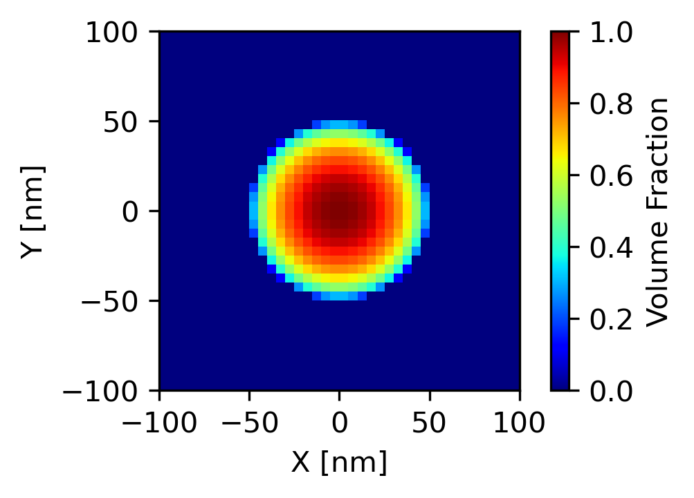
Figure 4: A zoomed-in view of the 2D projected sphere

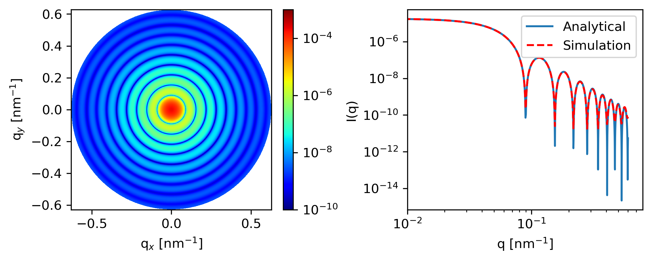
Figure 5: Results of the projected sphere case and comparison with analytical solution.

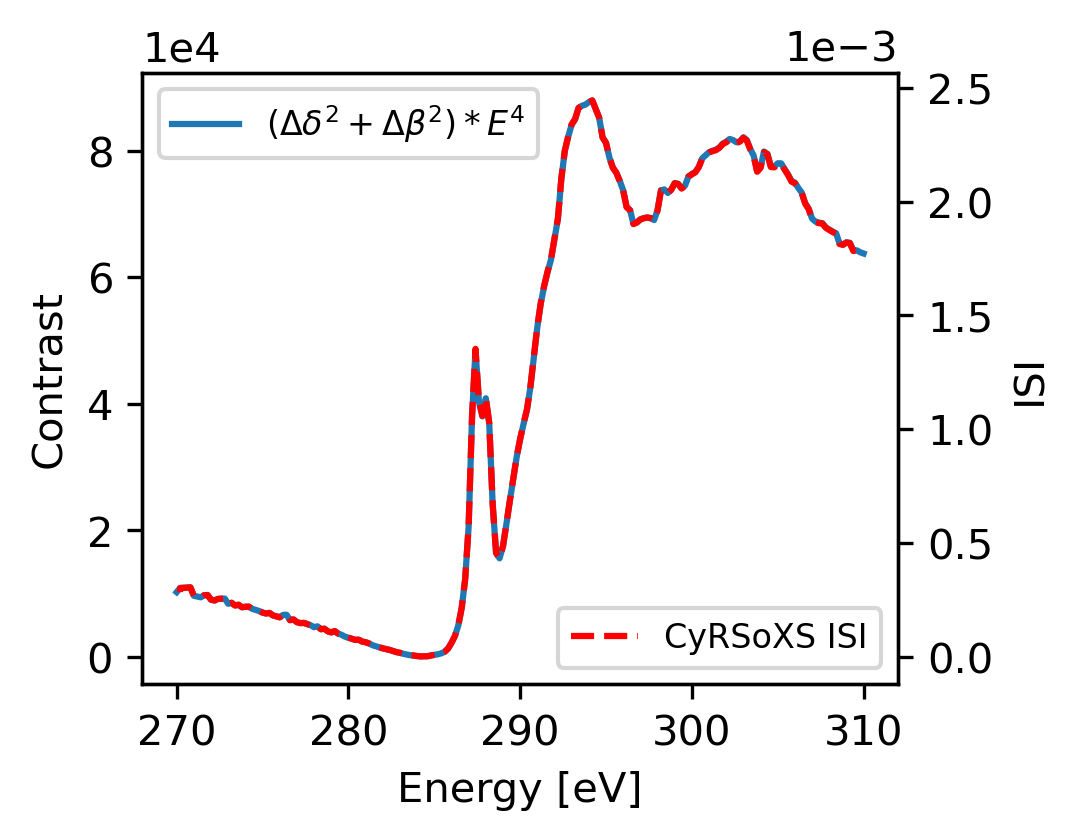
Figure 6: The simulated ISI alongside the theoretical energy dependence.

Fig. 5 shows the result of the 2D projected sphere validation case at 285 eV. Linecuts of the analytical and simulated data are plotted in Figure 5b and show excellent agreement. To validate the energy dependence of the P-RSoXS simulation, we calculate the integrated scattering intensity (ISI) across the range of simulated energy values. Fig. 6 plots the simulated ISI alongside the theoretical energy dependence given by the analytical expressions provided in Tatchev²⁴, computed for this specific dielectric function by us:

$$(\Delta\delta^{2}+\Delta\beta^{2})*E^{4}$$ (10)

While on different absolute scales, the theoretical and simulated energy dependence show commensurate relative scaling indicating we are capturing the correct physics in our scattering model.

5.1.2 3D sphere test

Fig. 7 shows the 3D sphere test domain along with a 2D slice of the sphere mid-plane. The morphology consists of $128\times 2048\times 2048$ voxels, where each voxel is $5\times 5\times 5$ nm³. A 3D sphere of radius 50 nm is placed at the center. The simulation was carried out at 285 eV, using tabulated polyethylene optical constants for the sphere and vacuum for the surrounding matrix.

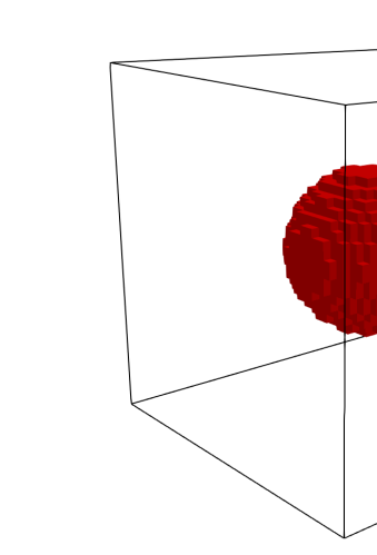
(a) 3D sphere

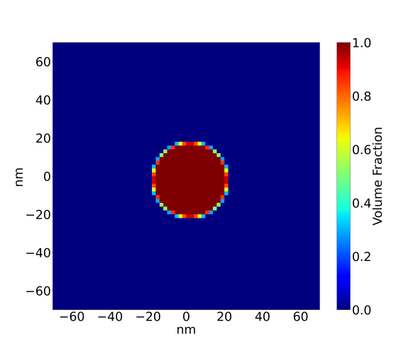
(b) 2D mid plane slice

Figure 7: Domain for the sphere validation test (not to scale) and a 2D slice along the mid plane.

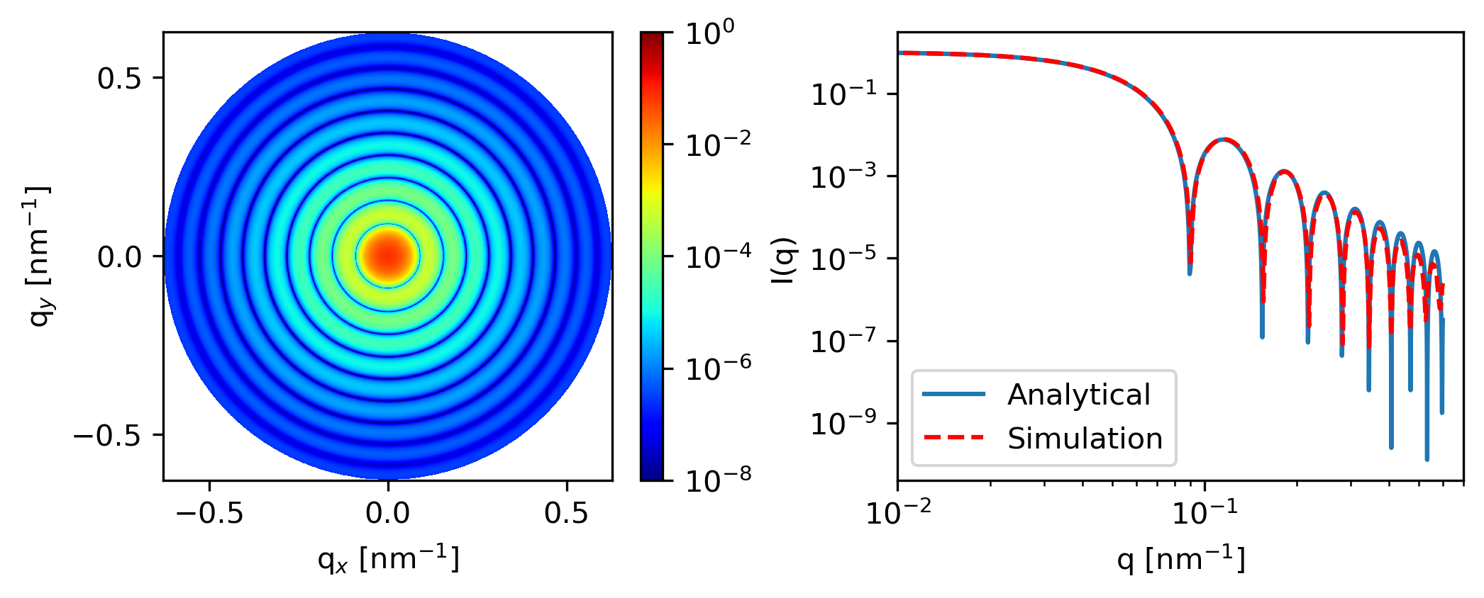
Figure 8: Results of the 3D sphere case and comparison with analytical solution.

Fig. 8a shows the 2D scattering pattern and Fig. 8b compares the 1D analytical expression for a sphere with the azimuthally integrated data from Fig. 8a. The analytical and simulation data were both normalized to 1 at q = 1e-2. We see an excellent comparison between the analytical and simulated results. The minor discrepancy between the simulation and analytical results at higher q values can be attributed to the finite discretization of the sphere and voxel size.

5.2 Periodic structure test

Extending beyond form factor scattering, many materials studied with X-ray scattering techniques exhibit periodic structures, which result in Bragg diffraction: constructive interference of the scattered X-rays produces sharp peaks at locations corresponding to the periodic spacing. Materials of this nature that have been studied with RSoXS include block copolymers ²⁵, ²⁶ and patterned thin films ²⁷. Voxelized representations will approximate the spacings and shapes of real morphologies. We perform two validation cases that reflect this periodic arrangement of structures: a) 2D hexagonal packed lattice; and b) grating test.

5.2.1 Circle on hexagonal lattice

We first consider an arrangement of circular domains on a 2D hexagonal lattice. This morphology is representative of hexagonally-packed cylinders, a common block copolymer morphology. We consider the cylinders to be oriented parallel to the X-ray beam.

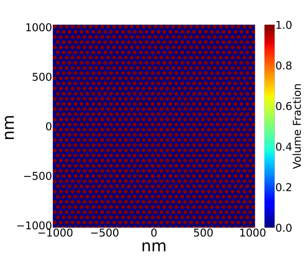
Figure 9: Volume fraction map of PEOlig for the hexagonal lattice. The dark blue region represents vacuum.

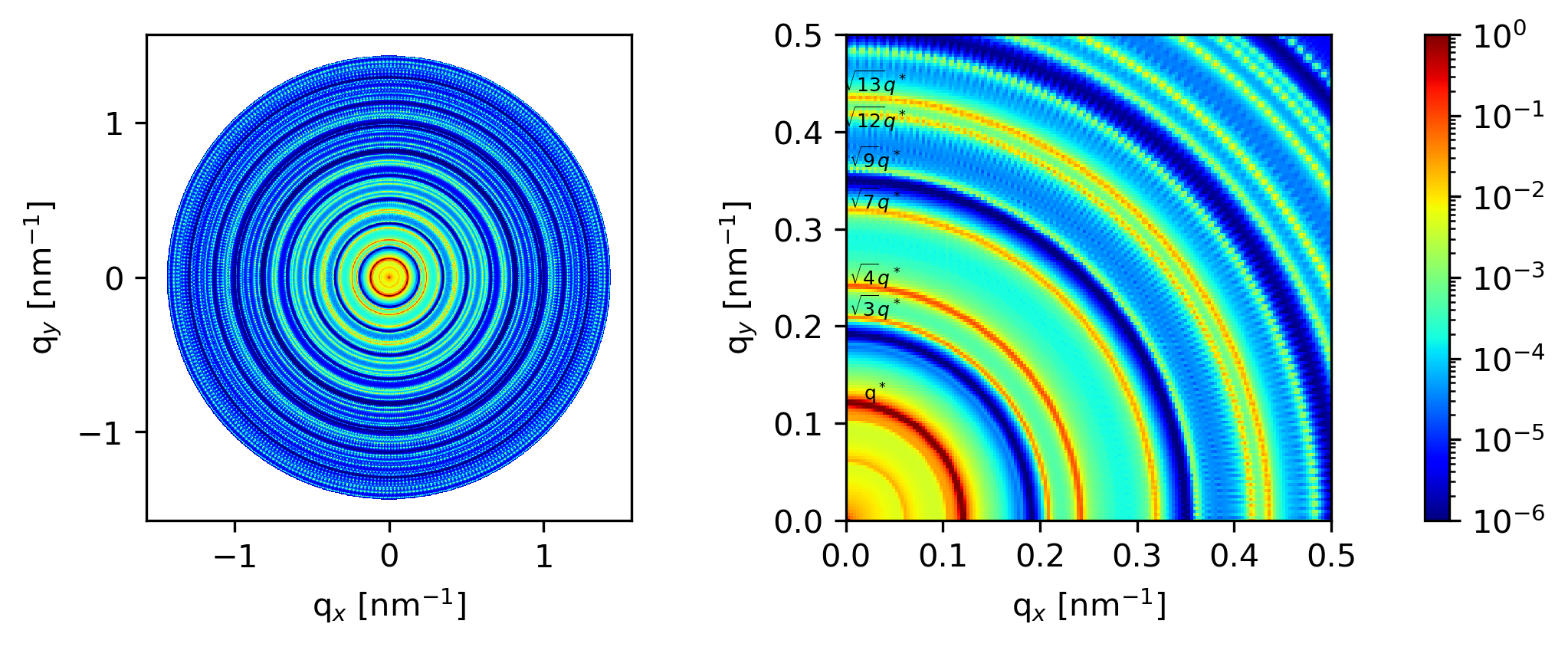
Figure 10: Hexagonal lattice validation case. Contours of I($\underline{\mathbf{q}}$) with the corresponding peak locations.

Fig. 10 shows the 2D scattering pattern output from Cy-RSoXS. Given the target lattice spacing of the input morphology, we observe Bragg peaks at the expected locations ($q^{*},\sqrt{3}q^{*},\sqrt{4}q^{*},\sqrt{7}q^{*},\sqrt{9}q^{*},$ and so on). Fig. 11 shows the azimuthally integrated scattering intensity plotted versus q, with the first 7 Bragg peaks labeled. There is perfect agreement between the analytical and simulated peak locations. We do observe some non-peak background features with low intensity that originate from the finite size of the model and voxel-level discretization effects. Such artifacts can be further reduced by using larger and/or higher-resolution models, models that contain realistic structural defects, and models with periodic boundary conditions.

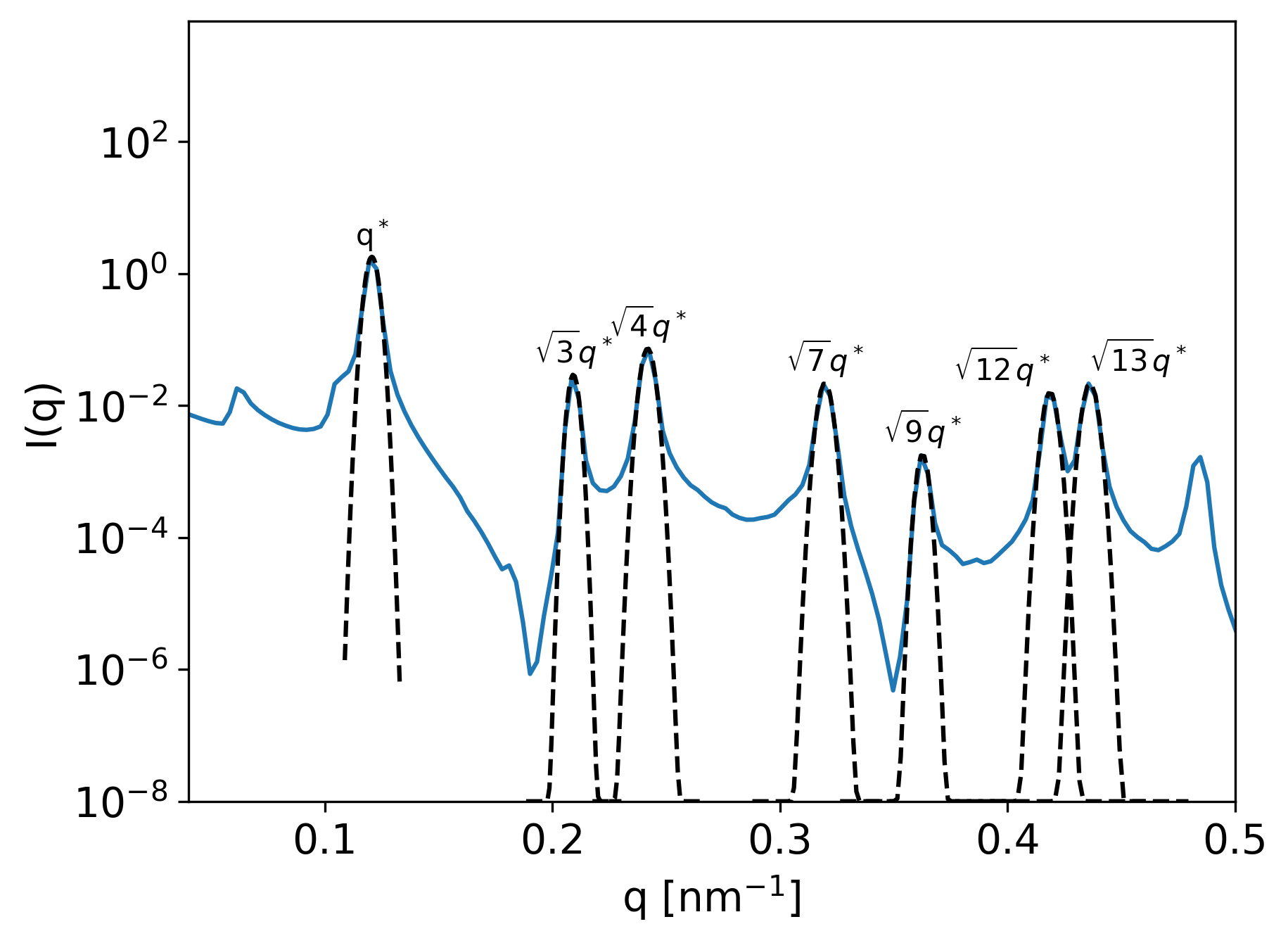
Figure 11: 1D simulated diffraction pattern with the analytical peak locations marked.

5.2.2 Grating test

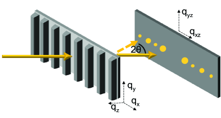
Figure 12: Setup of the line grating simulation

The second periodic structure test case is a set of parallel lines which form a grating structure. This type of morphology is observed in the directed self-assembly of block copolymers, or structures fabricated using lithographic processes; and is often seen in semiconducting manufacturing. We consider a single line grating morphology in 2D and 3D. The 3D morphology consists of single line grating extended in the Z direction. Fig. 12 shows the setup for the grating simulation. The 2D morphology consists of $1024\times 1024\times 1$ voxels whereas the 3D morphology consists of $1024\times 1024\times 63$ voxels, with each voxel representing a physical dimension of $1\times 1\times 1$ nm³. The simulation was carried out at 17 keV. The analytical results are calculated using a previously-published procedure ²⁸ in which the grating is discretized into a stack of trapezoids. The analytical solution for the Fourier Transform of a trapezoid is used to calculate the scattering intensity at each q position. Fig. 13 compares the analytical and simulation results for the line gratings. The simulated results are in excellent agreement with the analytical results.

(a) 2D Line gratings.

(b) 3D line gratings.

Figure 13: Comparison of analytical and simulation line cut integration for 2D and 3D line gratings. The $q_{x}$ component of $\underline{\mathbf{q}}$ is at the location of the first order peak.

5.3 Orientation effect on polymer-grafted nanoparticles

All of the previous test cases dealt with isotropic materials. As the final validation case, we consider a film of polymer-grafted nanoparticles (PGNs) ². Polystyrene chains are grafted onto gold nanoparticles, and the confinement of polystyrene chains near the nanoparticle surface results in radial stretching of the chains and a net molecular orientation. Fig. 14 is a 2D slice of the 3D morphology, showing the gold nanoparticle core surrounded by the oriented polystyrene shell, all embedded in a matrix of isotropic polystyrene. The CyRSoXS simulation is tested against the current state-of-the-art P-RSoXS simulator ¹⁰. Fig. 15 plots the scattering anisotropy at q = (0.02 to 0.04) nm^-1 and two energies for the reference simulator and our GPU-accelerated P-RSoXS simulator. Our implementation perfectly reproduces the results of the reference simulator.

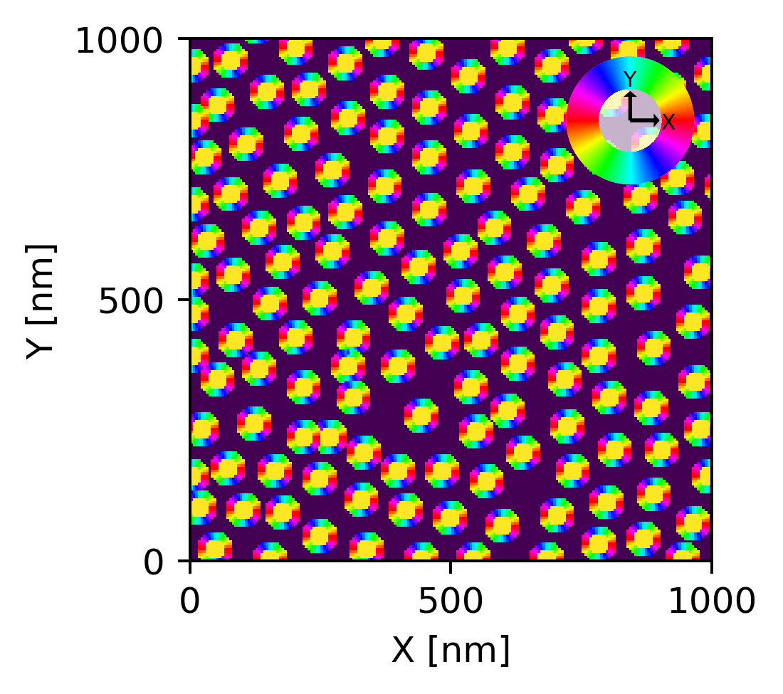
Figure 14: 2D slice of 3D polymer-grafted nanoparticle (PGN) morphology. An oriented shell of polystyrene (PS) surrounds each gold nanoparticle core. The pixels in this image are colored by the values of the Euler angle $\phi^{PS})$, which exhibits a radial orientation relative to the particle centers. The orientation of the extraordinary axis of the dielectric function in real space relative to the $x$ and $y$ axes is shown in the inset color wheel. This 2D slice was collected near the particle equators such that $\phi^{PS}$ $\approx$ $\pi/2$ for all pixels.

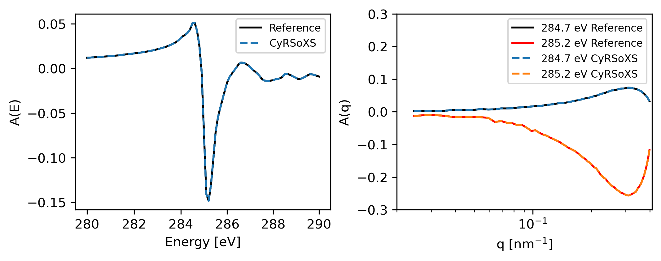
Figure 15: Scattering Anisotropy plotted versus select energies and q-values for the CyRSoXS and reference simulators

6 Performance

In this section, we report the scaling of CyRSoXS with respect to variation in number of voxels and materials. All computation was carried out using NVIDIA Voltas V-100 GPU with 32 GB of memory.

6.1 Performance with increasing number of voxels

As a first scaling test, we considered performance with increase in number of voxels. The overall number of voxels was varied from $128\times 128\times 16$ to $1024\times 1024\times 128$ with an increment of $2$ in each direction. The number of material is fixed to be 4 and the computation was carried out for 150 energy levels. For each energy level, Electric field $\underline{\mathbf{e}}$ was rotated from $0^{o}$ to $180^{o}$ at an increment of $2^{o}$.

(a) Total time with variation in number of voxels.

(b) Percentage of time with variation in number of voxels.

Figure 16: Performance of  Algorithm 1 with variation in number of voxels. The number of material was fixed to 4. The time reported corresponds to computation of 150 energy level with $\underline{\mathbf{e}}$ rotated from $0^{o}$ to $180^{o}$ at increment of $2^{o}$ for each energy level.

Fig. 16 compares the time with increase in the number of voxels for  Algorithm 1. Fig. 16(a) shows the variation of total wall-time with respect to the number of voxels. Overall we see a linear dependence ($\mathcal{O}(N)$), where $N$ is the total number of voxels. Fig. 16(b) compares the percentage of time taken by different sections of the computation. The total time mostly is dominated by polarization computation (Eq. (5)) and FFT computation. The “other” cost, which include Ewalds projection computation, image rotation and data transfer from CPU to GPU and vice–versa, form a significant fraction at lower resolution (i.e., smaller voxel sizes), but become insignificant at higher resolutions.

(a) Total time with variation in number of voxels

(b) Percentage of time with variation in number of voxels

Figure 17: Performance of  Algorithm 2 with variation in number of voxels. The number of material was fixed to 4. The time reported corresponds to computation of 150 energy level with $\underline{\mathbf{e}}$ rotated from $0^{o}$ to $180^{o}$ at increment of $2^{o}$ for each energy level.

Fig. 17 compares the time with increase in the number of voxels for  Algorithm 2. Fig. 17(a) shows the variation of total time whereas Fig. 17(b) compares the percentage of time with increase in the number of voxels. We observe a similar performance behavior compared to the  Algorithm 1, including $\mathcal{O}(N)$ scaling with increase in number of voxels. The majority of the time is spent in computing $\underline{\underline{\mathbf{N_{t}}}}$ which also involves the copying data from CPU to GPU (Algorithm 3), polarization computation and FFT computation. The “other” cost, similar to the previous algorithm, forms a significant chunk of percentage at lower resolution but becomes insignificant at higher resolutions.

6.2 Performance with increasing number of materials: Communication minimization vs memory minimization algorithms

As a next analysis, we compared the performance of both the algorithm with respect to increase in the number of materials. We considered a system with a voxel size of $2048\times 2048\times 64$. The computation was carried out for 9 energy levels. For each energy level, Electric field $\underline{\mathbf{e}}$ was rotated from $0^{o}$ to $180^{o}$ at an increment of $2^{o}$. We utilize 10 streams for the computation of  Algorithm 2 to overlap computation and communication.

Fig. 18(a) compares the total time for both the algorithm. We see  Algorithm 1 to be faster than the  Algorithm 2. However, the overall slope, or the rate of increase in time with material size tends to the much steeper for  Algorithm 1 compared to the  Algorithm 2. This is because the polarization computation (Eq. (5)) involves a loop over the number of material.  Algorithm 1 performs this computation for each rotation of $\underline{\mathbf{e}}$, whereas in case of  Algorithm 2, this computation is carried out once for each energy level and stored in $\underline{\underline{\mathbf{N_{t}}}}$. With increase in the number of material, this computation tends to dominate, and thus, we see a higher slope for  Algorithm 1. Further, we observe that the memory requirement of the  Algorithm 1 exceeds the overall GPU memory for material size $>4$, whereas  Algorithm 2 continues to give a linear variation with increase in material size. This agrees with the memory requirement analysis in  Section 4. We recall that memory requirement of Algorithm 1 exceeds Algorithm 2 for material size $\geq$ 3.

Fig. 18(b) shows the percentage of time for different sections of the  Algorithm 2. We see an increase in the time for $\underline{\underline{\mathbf{N_{t}}}}$ computation. This is expected as only $\underline{\underline{\mathbf{N_{t}}}}$ computation in  Algorithm 2 depends on the number of materials. Overall, the time is mostly dominated by FFT computations.

(a) Run-time

(b) Percentage of time for  Algorithm 2.

Figure 18: Run time and percentage distribution of  P-RSoXS for $2048\times 2048\times 64$ morphology with increasing number of material for 9 different energy levels. $\underline{\mathbf{e}}$ rotated from $0^{o}$ to $180^{o}$ at increment of $2^{o}$ for each energy level. For  Algorithm 1, the overall memory requirement exceeds the GPU memory size for number of material $>$ 4.

6.3 Scaling performance across multiple GPUs

We parallelize the code with respect to the energy level across multiple GPUs. This makes the code embarrassingly parallel. Each GPU device allocates its own chunk of memory depending on the energy levels owned by it and performs the computation independently. We utilize OpenMP to schedule the threads with each thread handling a single GPU. This allows us to utilize all GPUs efficiently across a single node.

In order to demonstrate the scaling performance, we consider a server with 2 NVIDIA V100 GPUs and analyzed the efficiency for different voxel sizes. We consider a material system with two different voxel size of $512\times 512\times 64$ and $1024\times 1024\times 128$ and 4 materials. We consider 150 energy levels distributed across multiple GPUs. Overall, we see an ideal scaling behavior with both algorithms achieving $2\times$ speedup while utilizing 2 GPUs.

(a) Scaling for $512\times 512\times 64$ voxel

(b) Scaling for $1024\times 1024\times 128$ voxel

Figure 19: Scaling of  P-RSoXS simulator on multiple GPU. The number of material was fixed to 4. The time reported corresponds to computation of 150 energy level distributed across multiple GPU with $\underline{\mathbf{e}}$ rotated from $0^{o}$ to $180^{o}$ at increment of $2^{o}$ for each energy level.

7 Python interface to CyRSoXS

In addition to GPU acceleration, we have added a python interface using Pybind11 ²⁹. Pybind11 was designed to expose C++ data types to Python and vice-versa. One of the benefits of this approach is directly passing the morphology information via memory instead of performing file IO operations, which can be a major bottleneck for fitting and other inverse problems. Additionally, the output of the scattering pattern in the form of NumPy arrays enables users to use sophisticated python visualization libraries like Matplotlib ³⁰, seaborn ³¹, and develop Python-based post-processing tools. We also interface with the cupy ³² library that enables morphology generation on GPU. A morphology generated on GPU can be directly passed to the simulator without copying data back and forth from the CPU. However, the morphology layout must strictly match the framework layout as shown in Fig. 3 and described in Section 4.1.

We believe that the availability of the Python interface will give a major boost to inverse problems relating to the material design, as most of the Machine Learning (ML) or Data analysis (DA) toolkits ^{33, 34, 35, 36} are currently Python-based. This interface will allow the users to seamlessly integrate their ML/DA models with the current framework.

8 Conclusion

We have demonstrated a new P-RSoXS virtual instrument with greatly increased performance compared to the state-of-the-art. Computations with this new virtual instrument are fast enough to enable practical data fitting by adjusting structure parameters using goal-seeking algorithms. The first fitting of orientational parameters to experimental P-RSoXS data was recently demonstrated using this virtual instrument to simulate polymer-grafted nanoparticles using a high-throughput multi-resolution parametric sweep of a 3-parameter system ². We have developed soon-to-be-published Python-driven workflows that demonstrate the practical use of this virtual instrument with other fitting methods, including genetic algorithm and Markov Chain Monte Carlo approaches. Close integration with Python environments affords opportunities to develop morphological models based on data fusion approaches, particularly leveraging real-space imaging, which reduces common questions of model uniqueness in fitting small-angle scattering data. The P-RSoXS virtual instrument shows great promise as a cornerstone of future approaches for assimilating complementary data streams to construct complex and self-consistent material structure representations in silico and ultimately to power inverse design frameworks that eliminate the need for costly Edisonian optimization approaches.

9 Acknowledgements

The authors acknowledge XSEDE grant number TG-CTS110007 for computing time and Iowa State University computing resources. KS and BG were supported in part by Office of Naval Research (ONR) Multiple University Research Initiative (MURI) 6119-ISU-ONR-2453. MLC and VGR acknowledge support by the National Science Foundation through Award No. DMR-1808622. VGR thanks the National Science Foundation Graduate Research Fellowship Program under Grant 1650114.

References

- Wessels and Jayaraman 2021 Wessels, M. G.; Jayaraman, A. Computational Reverse-Engineering Analysis of Scattering Experiments (CREASE) on Amphiphilic Block Polymer Solutions: Cylindrical and Fibrillar Assembly. Macromolecules 2021, 54, 783–796
- Mukherjee et al. 2021 Mukherjee, S.; Streit, J. K.; Gann, E.; Saurabh, K.; Sunday, D. F.; Krishnamurthy, A.; Ganapathysubramanian, B.; Richter, L. J.; Vaia, R. A.; DeLongchamp, D. M. Polarized X-ray scattering measures molecular orientation in polymer-grafted nanoparticles. Nature Communications 2021, 12, 1–10
- Pryor et al. 2017 Pryor, A.; Ophus, C.; Miao, J. A streaming multi-GPU implementation of image simulation algorithms for scanning transmission electron microscopy. Advanced structural and chemical imaging 2017, 3, 1–14
- Reynolds et al. 2022 Reynolds, V. G.; Callan, D. H.; Saurabh, K.; Murphy, E. A.; Albanese, K. R.; Chen, Y.-Q.; Wu, C.; Gann, E.; Hawker, C. J.; Ganapathysubramanian, B.; Bates, C. M.; Chabinyc, M. L. Simulation-guided analysis of resonant soft X-ray scattering for determining the microstructure of triblock copolymers. Molecular Systems Design & Engineering 2022,
- Axelrod et al. 2022 Axelrod, S.; Schwalbe-Koda, D.; Mohapatra, S.; Damewood, J.; Greenman, K. P.; Gómez-Bombarelli, R. Learning matter: Materials design with machine learning and atomistic simulations. Accounts of Materials Research 2022, 3, 343–357
- Vasudevan et al. 2021 Vasudevan, R.; Pilania, G.; Balachandran, P. V. Machine learning for materials design and discovery. 2021
- Guo et al. 2021 Guo, K.; Yang, Z.; Yu, C.-H.; Buehler, M. J. Artificial intelligence and machine learning in design of mechanical materials. Materials Horizons 2021, 8, 1153–1172
- Gomes et al. 2019 Gomes, C. P.; Selman, B.; Gregoire, J. M. Artificial intelligence for materials discovery. MRS Bulletin 2019, 44, 538–544
- Collins and Gann 2022 Collins, B. A.; Gann, E. Resonant soft X-ray scattering in polymer science. Journal of Polymer Science 2022, 60, 1199–1243
- Gann et al. 2016 Gann, E.; Collins, B. A.; Tang, M.; Tumbleston, J. R.; Mukherjee, S.; Ade, H. Origins of polarization-dependent anisotropic X-ray scattering from organic thin films. Journal of synchrotron radiation 2016, 23, 219–227
- Jiao et al. 2017 Jiao, X.; Ye, L.; Ade, H. Quantitative Morphology–Performance Correlations in Organic Solar Cells: Insights from Soft X-Ray Scattering. Advanced Energy Materials 2017, 7, 1700084
- Ye et al. 2016 Ye, L.; Jiao, X.; Zhao, W.; Zhang, S.; Yao, H.; Li, S.; Ade, H.; Hou, J. Manipulation of domain purity and orientational ordering in high performance all-polymer solar cells. Chemistry of Materials 2016, 28, 6178–6185
- Song et al. 2018 Song, X.; Gasparini, N.; Nahid, M. M.; Chen, H.; Macphee, S. M.; Zhang, W.; Norman, V.; Zhu, C.; Bryant, D.; Ade, H. A Highly Crystalline Fused-Ring n-Type Small Molecule for Non-Fullerene Acceptor Based Organic Solar Cells and Field-Effect Transistors. Advanced Functional Materials 2018, 28, 1802895
- Song et al. 2019 Song, X.; Gasparini, N.; Nahid, M. M.; Paleti, S. H. K.; Li, C.; Li, W.; Ade, H.; Baran, D. Efficient DPP Donor and Nonfullerene Acceptor Organic Solar Cells with High Photon-to-Current Ratio and Low Energetic Loss. Advanced Functional Materials 2019, 29, 1902441
- Mukherjee et al. 2017 Mukherjee, S.; Herzing, A. A.; Zhao, D.; Wu, Q.; Yu, L.; Ade, H.; DeLongchamp, D. M.; Richter, L. J. Morphological characterization of fullerene and fullerene-free organic photovoltaics by combined real and reciprocal space techniques. Journal of Materials Research 2017, 32, 1921–1934
- Litofsky et al. 2019 Litofsky, J. H.; Lee, Y.; Aplan, M. P.; Kuei, B.; Hexemer, A.; Wang, C.; Wang, Q.; Gomez, E. D. Polarized soft X-ray scattering reveals chain orientation within nanoscale polymer domains. Macromolecules 2019, 52, 2803–2813
- Attwood and Sakdinawat 2017 Attwood, D.; Sakdinawat, A. X-rays and extreme ultraviolet radiation: principles and applications; Cambridge university press, 2017
- Stöhr 1992 Stöhr, J. NEXAFS spectroscopy; Springer Science & Business Media, 1992; Vol. 25
- Mannsfeld 2012 Mannsfeld, S. C. In tune with organic semiconductors. Nature materials 2012, 11, 489–490
- Wang et al. 2010 Wang, C.; Hexemer, A.; Nasiatka, J.; Chan, E.; Young, A.; Padmore, H.; Schlotter, W.; Lüning, J.; Swaraj, S.; Watts, B. Resonant soft X-ray scattering of polymers with a 2D detector: Initial results and system developments at the Advanced Light Source. IOP Conf. Ser.: Mater. Sci. Eng. 2010; p 012016
- Watts 2014 Watts, B. Calculation of the Kramers-Kronig transform of X-ray spectra by a piecewise Laurent polynomial method. Optics Express 2014, 22, 23628–23639
- Born and Wolf 2013 Born, M.; Wolf, E. Principles of optics: electromagnetic theory of propagation, interference and diffraction of light; Elsevier, 2013
- Gann 2022 Gann, E. Optical-Constants-Database. 2022; https://github.com/EliotGann/Optical-Constants-Database
- Tatchev 2010 Tatchev, D. Multiphase approximation for small-angle scattering. Journal of Applied Crystallography 2010, 43, 8–11
- Wang et al. 2011 Wang, C.; Lee, D. H.; Hexemer, A.; Kim, M. I.; Zhao, W.; Hasegawa, H.; Ade, H.; Russell, T. P. Defining the nanostructured morphology of triblock copolymers using resonant soft X-ray scattering. Nano letters 2011, 11, 3906–3911
- Virgili et al. 2007 Virgili, J. M.; Tao, Y.; Kortright, J. B.; Balsara, N. P.; Segalman, R. A. Analysis of order formation in block copolymer thin films using resonant soft X-ray scattering. Macromolecules 2007, 40, 2092–2099
- Freychet et al. 2018 Freychet, G.; Cordova, I. A.; McAfee, T.; Kumar, D.; Pandolfi, R. J.; Anderson, C.; Naulleau, P.; Wang, C.; Hexemer, A. Using resonant soft x-ray scattering to image patterns on undeveloped resists. International Conference on Extreme Ultraviolet Lithography 2018. 2018; p 108090V
- Sunday et al. 2015 Sunday, D. F.; List, S.; Chawla, J. S.; Kline, R. J. Determining the shape and periodicity of nanostructures using small-angle x-ray scattering. Journal of Applied Crystallography 2015, 48, 1355–1363
- Jakob et al. 2019 Jakob, W.; Rhinelander, J.; Moldovan, D. pybind11–seamless operability between c++ 11 and python, 2017. URL https://github. com/pybind/pybind11 2019,
- Barrett et al. 2005 Barrett, P.; Hunter, J.; Miller, J. T.; Hsu, J.-C.; Greenfield, P. matplotlib–A Portable Python Plotting Package. Astronomical data analysis software and systems XIV. 2005; p 91
- Waskom et al. 2020 Waskom, M.; Botvinnik, O.; Gelbart, M.; Ostblom, J.; Hobson, P.; Lukauskas, S.; Gemperline, D. C.; Augspurger, T.; Halchenko, Y.; Warmenhoven, J. Seaborn: statistical data visualization. Astrophysics Source Code Library 2020, ascl–2012
- Nishino and Loomis 2017 Nishino, R.; Loomis, S. H. C. CuPy: A NumPy-compatible library for NVIDIA GPU calculations. 31st confernce on neural information processing systems 2017, 151
- Garreta and Moncecchi 2013 Garreta, R.; Moncecchi, G. Learning scikit-learn: machine learning in python; Packt Publishing Ltd, 2013
- Chollet 2018 Chollet, F. Keras: The python deep learning library. Astrophysics Source Code Library 2018, ascl–1806
- Abadi et al. 2016 Abadi, M.; Barham, P.; Chen, J.; Chen, Z.; Davis, A.; Dean, J.; Devin, M.; Ghemawat, S.; Irving, G.; Isard, M. Tensorflow: A system for large-scale machine learning. 12th USENIX symposium on operating systems design and implementation (OSDI 16). 2016; pp 265–283
- Paszke et al. 2019 Paszke, A.; Gross, S.; Massa, F.; Lerer, A.; Bradbury, J.; Chanan, G.; Killeen, T.; Lin, Z.; Gimelshein, N.; Antiga, L. Pytorch: An imperative style, high-performance deep learning library. arXiv preprint arXiv:1912.01703 2019,