Sandwiched Volterra Volatility model:
Markovian approximations and hedging

Abstract

We consider stochastic volatility dynamics driven by a general Hölder continuous Volterra-type noise and with unbounded drift. For such models, we consider the explicit computation of quadratic hedging strategies. While the theoretical solution is well-known in terms of the non-anticipating derivative for all square integrable claims, the fact that these models are typically non-Markovian provides a concrete difficulty in the direct computation of conditional expectations at the core of the explicit hedging strategy. To overcome this difficulty, we propose a Markovian approximation of the model which stems from an adequate approximation of the kernel in the Volterra noise. We study the approximation of the volatility, the prices as well as the optimal mean-square hedge and provide the corresponding error estimates. We complete the work with numerical simulations performed with different methods.

Keywords: stochastic volatility, sandwiched process, Hölder continuous noise, hedging, Monte Carlo methods
MSC 2020: 91G30; 60H10; 60H35; 60G22
Acknowledgements. The present research is carried out within the frame and support of the ToppForsk project nr. 274410 of the Research Council of Norway with title STORM: Stochastics for Time-Space Risk Models.

1 Introduction

A significant number of modern financial market models is characterized by the absence of the Markov property. Such a choice of modeling framework is substantiated by a number of empirical studies indicating presence of long memory in the market volatility. For instance, [15, 16] described the long-range dependence and volatility clustering effects which led to the development of models based on fractional Brownian motion with Hurst index $H>1/2$ such as [12, 13, 14]. Other empirical studies (see e.g. [28]) conclude that Hölder regularity of volatility is strictly less than $1/2$ and this statement gave birth to another class of non-Markovian “rough volatility” models such as rough Bergomi [8], SABR [25], Stein & Stein [29] or Heston [22] models. A substantial advantage of such models in comparison to the Markovian ones is the ability to grasp the implied volatility surface far more accurately and reproduce e.g. the power law of at-the-money volatility skew (see [4, 23, 24] or [40, Theorem 1]).

Another example of a non-Markovian market model – which the underlying model in this paper – is the Sandwiched Volterra Volatility (SVV) model introduced in [19]. Namely, we consider the financial market composed of the two primary assets:

• a risk-free bond (or bank account) with the price $e^{\int_{0}^{t}\nu(s)ds}$, $t\in[0,T]$, where $\nu\in C([0,T])$ is deterministic;

• a risky asset $S=\{S(t),~{}t\in[0,T]\}$, the risk-free dynamics of which is given by

  $$S(t) =S(0)+\int_{0}^{t}\nu(s)S(s)ds+\int_{0}^{t}Y(s)S(s)\left(\rho dB_{1}(s)+\sqrt{1-\rho^{2}}dB_{2}(s)\right),$$ (1.1)

  $$Y(t) =Y(0)+\int_{0}^{t}b(s,Y(s))ds+Z(t),$$ (1.2)

  where $S(0)$ and $Y(0)$ are given constants, $(B_{1},B_{2})=\{(B_{1}(t),B_{2}(t)),~{}t\in[0,T]\}$ is a standard 2-dimensional Brownian motion, $\rho\in(-1,1)$, $Z(t)=\int_{0}^{t}\mathcal{K}(t,s)dB_{1}(s)$ is a Hölder continuous Gaussian Volterra process. The discounted price of $S$ will be denoted by

  $$X(t):=e^{-\int_{0}^{t}\nu(s)ds}S(t),\quad t\in[0,T].$$ (1.3)

The drift $b=b(t,y)$ in (1.2) is unbounded and has an explosive growth to $+\infty$ whenever $y\to\varphi(t)+$ and explosive decay to $-\infty$ whenever $y\to\psi(t)-$, where $0<\varphi<\psi$ are two deterministic Hölder continuous functions. This structure ensures that the volatility process $Y=\{Y(t),~{}t\in[0,T]\}$ is sandwiched between $\varphi$ and $\psi$, i.e.

$$0<\varphi(t)<Y(t)<\psi(t),\quad t\in[0,T].$$ (1.4)

The property (1.4) guarantees that the volatility $Y$ stays strictly positive and that the price $S$ has moments of all orders. Note that the latter feature turns out to be crucial from the financial perspective: as noted in [5, Section 8], “several actively traded fixed-income derivatives require at least $L^{2}$ solutions to avoid infinite model prices”. And still, it is often absent even in classical stochastic volatility models such as the standard Heston model [5, Proposition 3.1]. Another advantage of (1.1)–(1.3) is the flexibility in the driving noise. In this work, $Z$ can be an arbitrary Hölder continuous Gaussian Volterra process which allows to reproduce multiple empirical phenomena: for example, taking

$$\mathcal{K}(t,s):=\frac{1}{\Gamma\left(H+\frac{1}{2}\right)}(t-s)^{H-\frac{1}{2}}\mathbbm{1}_{0\leq s\leq t\leq T}$$

gives long memory if $H>\frac{1}{2}$ and roughness if $H<\frac{1}{2}$ covering both modeling paradigms mentioned above. Furthermore, the setting of Gaussian Volterra processes is general enough to combine them as advocated in e.g. [3, Section 7.7] or [26].

While absence of Markovianity in stochastic volatility models is well supported by empirical evidence, we have to highlight that it also brings substantial difficulties from the point of view of stochastic methods, especially in optimization problems. As an example, consider a mean-square hedging problem of the form

$$\inf_{u}J(u):=\inf_{u}\mathbb{E}\left[\left(F-\int_{0}^{T}u(s)dX(s)\right)^{2}\right],$$ (1.5)

where the financial claim $F=F(X(T))\in L^{2}(\mathbb{P})$ and the infimum is taken over all $\mathbb{F}$-adapted $X$-integrable strategies with $\mathbb{F}=\{\mathcal{F}_{t},~{}t\in[0,T]\}$ being the filtration generated by $(B_{1},B_{2})$. From the theoretical perspective, the problem (1.5) is well understood: for martingale discounted prices $X$, the existence of the solution to (1.5) is guaranteed by the celebrated Galtchouk-Kunita-Watanabe decomposition theorem (see e.g. [36, 37]). Furthermore, if $X$ is additionally square integrable, [17] gives the explicit representation of the optimal hedging strategy: according to [17, Theorem 2.1], the solution to (1.5) can be written as the non-anticipating derivative $\mathfrak{D}F$ defined as the $L^{2}$-limit of simple processes

$$\begin{gathered}\mathfrak{D}F:=L^{2}\text{-}\lim_{|\pi|\to 0}u_{\pi},\\ u_{\pi}:=\sum_{k=0}^{n-1}\frac{\mathbb{E}\left[F\cdot(X(t_{k+1})-X(t_{k}))~{}|~{}\mathcal{F}_{t_{k}}\right]}{\mathbb{E}\left[(X(t_{k+1})-X(t_{k}))^{2}~{}|~{}\mathcal{F}_{t_{k}}\right]}\mathbbm{1}_{(t_{k},t_{k+1}]},\end{gathered}$$ (1.6)

where $|\pi|:=\max_{k}(t_{k}-t_{k-1})$ denotes the mesh of the partition $\pi=\{0=t_{0}<t_{1}<...<t_{n}=T\}$. Formula (1.6) is explicit in the sense that the hedge is written only in terms of the discounted price model, the information flow of reference, and the claim $F$. This formula is in the spirit of the Clarck-Haussmann-Ocone (CHO) formula (see e.g. [35, 21]) but we stress that (1.6) has several important advantages. Namely, the CHO formula exploits the Malliavin derivative which is tailored for specific noises (e.g. Brownian motion) and claims falling in the domain of the Malliavin operator. In turn, formula (1.6) is available for all square integrable claims and all square integrable martingales as discounted prices. Nevertheless, the practical use of (1.6) is still limited in many long memory and rough volatility models including the SVV model (1.2)–(1.3) due to the absence of the Markov property. Indeed, analytical expressions for $\mathfrak{D}F$ are usually impossible to obtain whereas dependence of $X$ on the past significantly complicates numerical computation of the conditional expectations in (1.6) by e.g. Monte Carlo methods.

In this paper, we tackle this problem by constructing a Markovian approximation to the SVV model (1.1)–(1.3) and then exploit it for the numerical computation of conditional expectations in (1.6). By doing this, we produce an algorithm for the computation of quadratic hedging strategies. The core of our approximation method lies in the following observation: since non-Markovianity in (1.1)–(1.3) comes from integrating the kernel $\mathcal{K}(t,s)$, we produce an approximation of $\mathcal{K}$ with a sequence of degenerate kernels $\{\mathcal{K}_{m},~{}m\geq 1\}$

$$\mathcal{K}_{m}(t,s)=\sum_{i=1}^{m}e_{m,i}(t)f_{m,i}(s),\quad 0\leq s\leq t\leq T,$$

where $e_{m,i}$ and $f_{m,i}$ are $L^{2}$ functions, so that the $(m+2)$-dimensional process

$$(X_{m},Y_{m},U_{m,1},...,U_{m,m})$$

given by

$$X_{m}(t) =X(0)+\int_{0}^{t}Y_{m}(s)X_{m}(s)\left(\rho dB_{1}(s)+\sqrt{1-\rho^{2}}dB_{2}(s)\right),$$ (1.7)

$$Y_{m}(t) =Y(0)+\int_{0}^{t}b(s,Y_{m}(s))ds+\sum_{i=1}^{m}e_{m,i}(t)U_{m,i}(t),$$

$$U_{m,1}(t) =\int_{0}^{t}f_{m,1}(s)dB_{1}(s),$$

$$~{}~{}\vdots$$

$$U_{m,m}(t) =\int_{0}^{t}f_{m,m}(s)dB_{1}(s),$$

is Markovian w.r.t. the filtration $\mathbb{F}=\{\mathcal{F}_{t},~{}t\in[0,T]\}$. Note that a similar idea was already utilized in [10] for the Riemann–Liouville fractional Brownian motion, in [1] for the rough Heston, and in [9] for the fractionally integrated standard Heston models, as well as in [2] in the context of optimal control in more general stochastic Volterra systems.

However, there are two main challenges related to application of such an approach in the setting (1.1)–(1.3). First of all, the drift $b$ in (1.2) is unbounded which creates substantial technical difficulties in estimating the error between the original model and its approximation. Second, in order to ensure existence and uniqueness of $Y_{m}$ from (1.7), it is necessary to demand that the Hölder regularity of the process $Z_{m}(t):=\sum_{i=1}^{m}e_{m,i}(t)U_{m,i}(t)$ is the same as the one of the original noise $Z$ or higher.

In this paper, we deal with the first challenge by using the pathwise bounds for sandwiched processes developed in [20] whereas the second issue is addressed by imposing more restrictive requirements on the approximating sequence $\{\mathcal{K}_{m},~{}m\geq 1\}$. As examples, we provide explicit sequences for the rough fractional and the general Hölder continuous kernels. Once obtained the approximation $X_{m}$ of the discounted price $X$, we plug it into (1.6) and prove the $L^{1}$–convergence of

$$u_{\pi}^{m}:=\sum_{k=0}^{n-1}\frac{\mathbb{E}\left[F_{m}(X_{m}(t_{k+1})-X_{m}(t_{k}))~{}|~{}\mathcal{F}_{t_{k}}\right]}{\mathbb{E}\left[(X_{m}(t_{k+1})-X_{m}(t_{k}))^{2}~{}|~{}\mathcal{F}_{t_{k}}\right]}\mathbbm{1}_{(t_{k},t_{k+1}]},\quad F_{m}:=F(X_{m}(T))$$ (1.8)

to the optimal hedge $\mathfrak{D}F$ when $\mathcal{K}(t,s)=\mathcal{K}(t-s)$.

Note that the conditional expectations in (1.8) simplify as

$$\mathbb{E} \left[F(X_{m}(T))(X_{m}(t_{k+1})-X_{m}(t_{k}))~{}|~{}\mathcal{F}_{t_{k}}\right]$$

$$=\mathbb{E}\left[F(X_{m}(T))(X_{m}(t_{k+1})-X_{m}(t_{k}))~{}|~{}X_{m}(t_{k}),~{}Y_{m}(t_{k}),~{}U_{m,1}(t_{k}),...,U_{m,m}(t_{k})\right]$$

$$=:\Phi_{1}(t_{k},X_{m}(t_{k}),Y_{m}(t_{k}),U_{m,1}(t_{k}),...,U_{m,m}(t_{k})),$$

$$\mathbb{E} \left[(X_{m}(t_{k+1})-X_{m}(t_{k}))^{2}~{}|~{}\mathcal{F}_{t_{k}}\right]$$

$$=\mathbb{E}\left[(X_{m}(t_{k+1})-X_{m}(t_{k}))^{2}~{}|~{}X_{m}(t_{k}),~{}Y_{m}(t_{k}),~{}U_{m,1}(t_{k}),...,U_{m,m}(t_{k})\right]$$

$$=:\Phi_{2}(t_{k},X_{m}(t_{k}),Y_{m}(t_{k}),U_{m,1}(t_{k}),...,U_{m,m}(t_{k})),$$

with $\Phi_{1}$ and $\Phi_{2}$ being two measurable functions. Therefore, the problem of searching for the optimal hedge boils down to computation of $\Phi_{1}$ and $\Phi_{2}$. We use numerical schemes for the SVV model from [18, 19] and provide two Monte Carlo algorithms to estimate these conditional expectations: the Nested Monte Carlo and the Least Squares Monte Carlo.

The paper is organized as follows. Section 2 contains the detailed descriprion of the SVV model (1.1)–(1.3) and gathers some necessary known results. Section 3 provides estimates of an error between the original model $(X,Y)$ and $(X_{m},Y_{m})$ obtained by replacing the kernel in the volatility with a general approximant $\mathcal{K}_{m}$. In Section 4, we describe the actual construction of the Markovian approximation and illustrate the approach with two examples of rough fractional and general Hölder continuous kernels. Section 5 concentrates on the mean-variance hedging problem (1.5), the description of two Monte Carlo approaches for computation of the non-anticipating derivative as well as simulations.

2 Market modeling with the SVV and quadratic hedging

Hereafter we specify the model (1.1)–(1.3) on the complete probability space $(\Omega,\mathcal{F},\mathbb{P})$ in more detail and then collect some fundamental results for the upcoming discussion and recall the concept of non-anticipating derivative within quadratic hedging. Before proceeding to the main content, let us introduce some notation used in the sequel.

Notation.

1. We denote by $\mathbb{F}=\{\mathcal{F}_{t},~{}t\in[0,T]\}$, $T<\infty$, the $\mathbb{P}$-augmented filtration generated by the 2-dimensional Brownian motion $(B_{1},B_{2})=\{(B_{1}(t),B_{2}(t)),~{}t\in[0,T]\}$ from (1.1)–(1.3).

2. In what follows, by $C$ we will denote any positive deterministic constant the exact value of which is not important in the context. Note that $C$ may change from line to line (or even within one line).

3. Throughout the paper, $L^{2}(\mathbb{P})$ will denote a standard space of square-integrable random variables. For a given square-integrable martingale $\eta=\{\eta(t),~{}t\in[0,T]\}$, the Hilbert space of stochastic processes such that

   $$\lVert u\rVert_{L^{2}(\mathbb{P}\times[\eta])}:=\left(\mathbb{E}\left[\int_{0}^{T}u^{2}(s)d[\eta](s)\right]\right)^{\frac{1}{2}}<\infty$$

   will be denoted by $L^{2}(\mathbb{P}\times[\eta])$.

2.1 Stochastic volatility process

First of all, we describe the driving noise $Z$ in (1.2). Consider a function $\mathcal{K}$: $[0,T]^{2}\to\mathbb{R}$ that satisfies the following assumption.

Assumption (K).

The function $\mathcal{K}$: $[0,T]^{2}\to\mathbb{R}$ is a Volterra kernel, i.e. $\mathcal{K}(t,s)=0$ whenever $t<s$, and the following conditions hold:

• $\mathcal{K}$ is square integrable, i.e.

  $$\int_{0}^{T}\int_{0}^{T}\mathcal{K}^{2}(t,s)dsdt=\int_{0}^{T}\int_{0}^{t}\mathcal{K}^{2}(t,s)dsdt<\infty,$$

  and, moreover,

  $$\int_{0}^{T}\mathcal{K}^{2}(t,s)ds<\infty\quad\forall t\in[0,T];$$

• there exists a constant $H\in(0,1)$ such that, for any $\lambda\in(0,H)$,

  $$\int_{0}^{t}(\mathcal{K}(t,u)-\mathcal{K}(s,u))^{2}du\leq\ell_{\lambda}^{2}|t-s|^{2\lambda},\quad 0\leq s\leq t\leq T,$$

  where $\ell_{\lambda}>0$ is a constant, possibly dependent on $\lambda$.

By means of $\mathcal{K}$, we now define a Gaussian Volterra process $Z=\{Z(t),~{}t\in[0,T]\}$ as

$$Z(t):=\int_{0}^{t}\mathcal{K}(t,s)dB_{1}(s),\quad t\in[0,T],$$ (2.1)

and immediately remark that

• (K1) ensures that the stochastic integral in (2.1) is well-defined for all $t\in[0,T]$,

• (K2) guarantees (see e.g. [7, Theorem 1 and Corollary 4]) that $Z$ has a modification that is Hölder continuous of any order $\lambda\in(0,H)$. Moreover, for any $\lambda\in(0,H)$, the positive random variable $\Lambda=\Lambda_{\lambda}$ such that

  $$|Z(t)-Z(s)|\leq\Lambda|t-s|^{\lambda},\quad t,s\in[0,T],$$ (2.2)

  can be chosen to have moments of all orders. In what follows, such Hölder continuous modification as well as $\Lambda$ with all the moments will be used.

In this paper, we mostly deal with difference kernels in the Volterra noise $Z$. Before proceeding further, let us give two relevant examples.

Example 2.1.

(Hölder continuous kernels) Let $\mathcal{K}(t,s)=\mathcal{K}(t-s)\mathbbm{1}_{0\leq s\leq t\leq T}$ for some function $\mathcal{K}\in C([0,T])$. Assume also that $\mathcal{K}$ is $H$-Hölder continuous for some $H\in(0,1)$. Then

$$\int_{0}^{t} (\mathcal{K}(t,u)-\mathcal{K}(s,u))^{2}du$$

$$=\int_{0}^{s}(\mathcal{K}(t-u)-\mathcal{K}(s-u))^{2}du+\int_{s}^{t}(\mathcal{K}(t-u)-\mathcal{K}(0)+\mathcal{K}(0))^{2}du$$

$$\leq C\int_{0}^{s}|t-s|^{2H}du+C\int_{0}^{t-s}u^{2H}du+C\int_{0}^{t-s}\mathcal{K}^{2}(0)du$$

$$\leq C|t-s|^{2\left(H\wedge\frac{1}{2}\right)},$$

i.e. (K2) is satisfied and the process

$$Z(t)=\int_{0}^{t}\mathcal{K}(t-s)dB_{1}(s),\quad t\in[0,T],$$

has a modification that is Hölder continuous up to the order $H\wedge\frac{1}{2}$. Furthermore, if additionally $\mathcal{K}(0)=0$, then it is easy to see that

$$\mathbb{E}[(Z(t)-Z(s))^{2}]=\int_{0}^{t}(\mathcal{K}(t,u)-\mathcal{K}(s,u))^{2}du\leq C|t-s|^{2H},$$

i.e. $Z$ has a modification that is Hölder continuous up to the order $H$.

Example 2.2.

(Fractional kernel) Let $\mathcal{K}(t,s)=\frac{1}{\Gamma\left(H+\frac{1}{2}\right)}(t-s)^{H-\frac{1}{2}}\mathbbm{1}_{0\leq s\leq t\leq T}$ with $H\in\left(0,1\right)$. The process

$$Z(t)=\frac{1}{\Gamma\left(H+\frac{1}{2}\right)}\int_{0}^{t}(t-s)^{H-\frac{1}{2}}dB_{1}(s),\quad t\in[0,T],$$

is called the Riemann-Liouville fractional Brownian motion (RL-fBm) and it is well-known (see e.g. [39, Lemma 3.1]) that, for any $s<t$,

$$\mathbb{E}[(Z(t)-Z(s))^{2}] =\frac{1}{\Gamma^{2}\left(H+\frac{1}{2}\right)}\int_{0}^{s}\left((t-u)^{H-\frac{1}{2}}-(s-u)^{H-\frac{1}{2}}\right)^{2}du$$

$$\quad+\frac{1}{\Gamma^{2}\left(H+\frac{1}{2}\right)}\int_{0}^{t-s}u^{2H-1}du$$

$$\leq C|t-s|^{2H}$$

for some constant $C$. Thus (K2) holds and the RL-fBm has a modification that is Hölder continuous up to the order $H$.

For a given pair $\varphi$, $\psi$: $[0,T]\to\mathbb{R}$ such that $\varphi(t)<\psi(t)$, $t\in[0,T]$, and any $a_{1}$, $a_{2}\geq 0$, we introduce the notation $\mathcal{D}_{a_{1},a_{2}}$ for the set

$$\mathcal{D}_{a_{1},a_{2}}:=\{(t,y)\in[0,T]\times\mathbb{R}_{+},~{}y\in(\varphi(t)+a_{1},\psi(t)-a_{2})\}.$$

Consider a stochastic process $Y=\{Y(t),~{}t\in[0,T]\}$ defined by (1.2), where the initial value $Y(0)$ and the drift $b$ satisfy the following assumption.

Assumption (Y).

There exist $H$-Hölder continuous functions $\varphi$, $\psi$: $[0,T]\to\mathbb{R}$, $0<\varphi(t)<\psi(t)$, $t\in[0,T]$, with $H$ being the same as in (K2) such that

• $Y(0)$ is deterministic and $0<\varphi(0)<Y(0)<\psi(0)$,

• $b$: $\mathcal{D}_{0,0}\to\mathbb{R}$ is continuous and, moreover, for any $\varepsilon\in\left(0,\min\left\{1,\frac{1}{2}\lVert\psi-\varphi\rVert_{\infty}\right\}\right)$

  $$|b(t_{1},y_{1})-b(t_{2},y_{2})|\leq\frac{c_{1}}{\varepsilon^{p}}\left(|y_{1}-y_{2}|+|t_{1}-t_{2}|^{H}\right),\quad(t_{1},y_{1}),(t_{2},y_{2})\in\mathcal{D}_{\varepsilon,\varepsilon},$$

  where $c_{1}>0$ and $p>1$ are given constants,

• $$b(t,y)\geq\frac{c_{2}}{(y-\varphi(t))^{\gamma}},\quad(t,y)\in\mathcal{D}_{0,0}\setminus\mathcal{D}_{y_{*},0},$$

  $$b(t,y)\leq-\frac{c_{2}}{(\psi(t)-y)^{\gamma}},\quad(t,y)\in\mathcal{D}_{0,0}\setminus\mathcal{D}_{0,y_{*}},$$

  where $y_{*}$, $c_{2}>0$ are given constants and $\gamma>\frac{1}{H}-1]$,

• the partial derivative $\frac{\partial b}{\partial y}$ with respect to the spacial variable exists, is continuous and

  $$-c_{3}\left(1+\frac{1}{(y-\varphi(t))^{q}}+\frac{1}{(\psi(t)-y)^{q}}\right)<\frac{\partial b}{\partial y}(t,y)<c_{3},\quad(t,y)\in\mathcal{D}_{0,0},$$

  for some $c_{3}>0$ and $q>0$.

According to [20], Assumptions (K) and (Y) together ensure that the SDE (1.2) has a unique solution that is sandwiched, i.e.

$$\varphi(t)<Y(t)<\psi(t),\quad t\in[0,T].$$ (2.3)

This and other relevant results from [20] regarding the process (1.2) are summarized in the following statement.

Theorem 2.3.

Let Assumptions (K) and (Y) hold. Then

• the SDE (1.2) has a unique strong solution $Y$ and (2.3) holds with probability 1;

• for any $\lambda\in\left(\frac{1}{1+\gamma},H\right)$, where $H$ is from (K2), there exist deterministic constants $L_{1}$ and $L_{2}>0$ (depending only on $Y(0)$, the shape of $b$ and $\lambda$) such that, with probability 1,

  $$\varphi(t)+\frac{L_{1}}{(L_{2}+\Lambda)^{\frac{1}{\gamma\lambda+\lambda-1}}}\leq Y(t)\leq\psi(t)-\frac{L_{1}}{(L_{2}+\Lambda)^{\frac{1}{\gamma\lambda+\lambda-1}}},\quad\quad t\in[0,T],$$ (2.4)

  where $\Lambda$ is from (2.2) and $\gamma$ is from (Y3);

• for any $r\in\mathbb{R}$,

  $$\mathbb{E}\left[\sup_{t\in[0,T]}\frac{1}{(Y(t)-\varphi(t))^{r}}\right]<\infty,\quad\mathbb{E}\left[\sup_{t\in[0,T]}\frac{1}{(\psi(t)-Y(t))^{r}}\right]<\infty.$$

Having in mind property (2.3), we will refer to the process $Y=\{Y(t),~{}t\in[0,T]\}$ defined by (1.2) as a sandwiched process.

2.2 Price process

Let Assumptions (K) and (Y) hold, $Z$ be a Gaussian Volterra process (2.1), and $Y=\{Y(t),~{}t\in[0,T]\}$ be the sandwiched process (1.2) such that (2.3) holds for some functions $0<\varphi<\psi$. We now consider the model introduced in Section 1 with a risk-free asset $e^{\int_{0}^{t}\nu(s)ds}$ and a risky asset $S=\{S(t),~{}t\in[0,T]\}$ defined by (1.1), where $S(0)>0$ is some deterministic constant and $\rho\in(-1,1)$. Clearly, the process $X$ defined by (1.3) satisfies the SDE

$$X(t)=X(0)+\int_{0}^{t}Y(s)X(s)\left(\rho dB_{1}(t)+\sqrt{1-\rho^{2}}dB_{2}(t)\right),\quad t\in[0,T],$$ (2.5)

where, for notational simplicity, we denote $X(0):=S(0)$. Moreover, the following Theorem holds.

Theorem 2.4.

([19, Theorem 2.6])

• Equation (1.1) has a unique strong solution and

  $$S(t)=S(0)\exp\left\{\int_{0}^{t}\left(\nu(s)-\frac{Y^{2}(s)}{2}\right)ds+\int_{0}^{t}Y(s)\left(\rho dB_{1}(t)+\sqrt{1-\rho^{2}}dB_{2}(t)\right)\right\}.$$

  In particular,

  $$X(t)=X(0)\exp\left\{-\int_{0}^{t}\frac{Y^{2}(s)}{2}ds+\int_{0}^{t}Y(s)\left(\rho dB_{1}(t)+\sqrt{1-\rho^{2}}dB_{2}(t)\right)\right\}.$$

• For any $r\in\mathbb{R}$,

  $$\mathbb{E}\left[\sup_{t\in[0,T]}S^{r}(t)\right]<\infty,\quad\mathbb{E}\left[\sup_{t\in[0,T]}X^{r}(t)\right]<\infty.$$ (2.6)

Remark 2.5.

Theorem 2.4 implies that $X=\{X(t),~{}t\in[0,T]\}$ is a square integrable martingale w.r.t. the filtration $\mathbb{F}=\{\mathcal{F}_{t},~{}t\in[0,T]\}$ generated jointly by $B_{1}$ and $B_{2}$.

Remark 2.6.

We stress that (2.6) does not hold in general even in classical stochastic volatility models such as the Heston model (see e.g. [5]). This has repercussions in the possibilities of numerical simulations as well as in various applications such as pricing hedging or portfolio optimization. In our case, the existence of moments of all orders is achieved thanks to the boundedness of $Y$.

We conclude the Subsection with a result on regularity of the probability laws of $S$ and $X$ presented in [19].

Theorem 2.7.

[19, Theorem 3.8] For any $t\in(0,T]$, the law of $S(t)$ (and consequently of $X(t)=e^{-\int_{0}^{t}\nu(s)ds}S(t)$) has continuous and bounded density.

2.3 Quadratic hedging: some considerations

Let Assumptions (K) and (Y) hold, $S=\{S(t),~{}t\in[0,T]\}$ be defined by (1.1) and $X(t):=e^{-\int_{0}^{t}\nu(s)ds}S(t)$. In what follows, we discuss mean-square hedging problem and in this Subsection we provide some known theoretical background for that. We are interested in European options with rather complicated payoffs $F:=F(X(T))$ covering both classical contracts (such as standard call options) and exotic ones with discontinuities in $F$ (digital, supershare, binary, truncated payoff options and so on). Namely, the payoff function $F$: $\mathbb{R}_{+}\to\mathbb{R}$ satisfies the following assumption.

Assumption (F).

The payoff function $F$: $\mathbb{R}_{+}\to\mathbb{R}$ can be represented as

$$F=F_{1}+F_{2},$$

where

• $F_{1}$ is globally Lipschitz, i.e. there exists $C>0$ such that

  $$|F_{1}(t)-F_{1}(s)|\leq C|t-s|,\quad s,t\geq 0;$$

• $F_{2}$: $\mathbb{R}_{+}\to\mathbb{R}$ is of bounded variation over $\mathbb{R}_{+}$, i.e.

  $$V(F_{2}):=\lim_{x\to\infty}V_{[0,x]}(F_{2})<\infty,$$

  where

  $$V_{[0,x]}(F_{2}):=\sup\sum_{j=1}^{N}|F_{2}(x_{j})-F_{2}(x_{j-1})|$$

  and the supremum above is taken over all $N\geq 0$ and all partitions $0=x_{0}<x_{1}<...<x_{N}=x$.

In what follows, we will need to approximate the discounted price $X(T)$ by a random variable $X_{m}(T)$ with “better” properties and then compare $F=F(X(T))$ with $F_{m}:=F(X_{m}(T))$. In order to do that, the following Theorem will be used.

Theorem 2.8.

Let $F=F_{1}+F_{2}$ satisfy Assumption (F) and $\xi$, $\hat{\xi}\in L^{r}(\mathbb{P})$, $1\leq r<\infty$. Then

• there exists a constant $C>0$ depending only on $F_{1}$ and $r$ such that

  $$\mathbb{E}[|F_{1}(\xi)-F_{1}(\hat{\xi})|^{r}]\leq C\mathbb{E}[|\xi-\hat{\xi}|^{r}];$$

• if $\xi$ has bounded density $f_{\xi}$, then

  $$\mathbb{E}[|F_{2}(\xi)-F_{2}(\hat{\xi})|^{r}]\leq 3^{r+1}V^{r}(F_{2})(\sup f_{\xi})^{\frac{r}{r+1}}\left(\mathbb{E}\left[|\xi-\hat{\xi}|^{r}\right]\right)^{\frac{r}{r+1}};$$ (2.7)

• if $\xi$ has bounded density $f_{\xi}$, then there exists a constant $C>0$ depending only on $F_{1}$, $F_{2}$, $r$ and the density $f_{\xi}$ such that

  $$\mathbb{E}[|F(\xi)-F(\hat{\xi})|^{r}]\leq C\left(\mathbb{E}[|\xi-\hat{\xi}|^{r}]+\left(\mathbb{E}\left[|\xi-\hat{\xi}|^{r}\right]\right)^{\frac{r}{r+1}}\right).$$

Proof.

Item 1) is obvious and follows directly from the Lipschitz condition for $F_{1}$. Item 2) is proved in [6, Theorem 2.4]. Item 3) is simply a combination of 1) and 2). ∎

Next, consider a quadratic hedging problem of minimizing the functional $J$ defined by (1.5) over all $\mathbb{F}$-adapted stochastic processes $u\in L^{2}(\mathbb{P}\times[X])$. By Theorem 2.4, the discounted price $X$ is a square integrable martingale w.r.t. the filtration $\mathbb{F}$ and hence [17] states that the unique minimizer of $J$ is equal to the non-anticipating derivative $\mathfrak{D}F$ of $F$ w.r.t. $X$. We give the necessary details regarding the non-anticipating derivatives below.

Let $\xi\in L^{2}(\mathbb{P})$ and $\eta=\{\eta(t),~{}t\in[0,T]\}$ be a square-integrable martingale w.r.t. a filtration $\{\mathcal{G}_{t},~{}t\in[0,T]\}$. For an arbitrary partition $\pi=\{0=t_{0}<t_{1}<...<t_{n}=T\}$ of $[0,T]$ with the mesh $|\pi|:=\max_{k}(t_{k}-t_{k-1})$, denote

$$u_{\pi} :=\sum_{k=0}^{n-1}u_{\pi,k}\mathbbm{1}_{(t_{k},t_{k+1}]},$$ (2.8)

$$u_{\pi,k} :=\frac{\mathbb{E}\left[\xi(\eta(t_{k+1})-\eta(t_{k}))~{}|~{}\mathcal{G}_{t_{k}}\right]}{\mathbb{E}\left[(\eta(t_{k+1})-\eta(t_{k}))^{2}~{}|~{}\mathcal{G}_{t_{k}}\right]},\quad k=0,1,...,n-1.$$

Definition 2.9.

Consider a monotone sequence of partitions $\{\pi_{M},~{}M\geq 1\}$, such that $|\pi_{M}|\to 0$ as $M\to\infty$. The $L^{2}(\mathbb{P}\times[\eta])$-limit

$$\mathfrak{D}\xi:=\lim_{|\pi_{M}|\to 0}u_{\pi_{M}}$$ (2.9)

is called the non-anticipating derivative of $\xi$ w.r.t. $\eta$.

The next result shows that $\mathfrak{D}\xi$ is well-defined and $\int_{0}^{T}\mathfrak{D}\xi(s)d\eta(s)$ gives the orthogonal $L^{2}(\mathbb{P}\times[\eta])$-projection of $\xi$ on the subspace of stochastic integrals w.r.t. $\eta$. By this, it is easy to see that the linear operator $\mathfrak{D}$ is actually the dual of the Itô integral.

Theorem 2.10.

([17, Theorem 2.1]) The non-anticipating derivative $\mathfrak{D}\xi$ is well-defined, i.e. the limit (2.9) exists and does not depend on the particular choice of the partitions. Moreover, any $\xi\in L^{2}(\mathbb{P})$ admits a unique representation of the form

$$\xi=\xi_{0}+\int_{0}^{T}\mathfrak{D}\xi(s)d\eta(s),$$

where $\xi_{0}\in L^{2}(\mathbb{P})$ is such that $\mathfrak{D}\xi_{0}=0$ and $\mathbb{E}\left[\xi_{0}\int_{0}^{T}\mathfrak{D}\xi(s)d\eta(s)\right]=0$.

Notation.

Since the limit (2.9) does not depend on the particular choice of partition $\{\pi_{M},~{}M\geq 1\}$, we will use the notation

$$\mathfrak{D}\xi:=\lim_{|\pi|\to 0}u_{\pi},$$

meaning that the limit in $L^{2}(\mathbb{P}\times[\eta])$ is taken along an arbitrary sequence of monotone partitions with the mesh going to zero.

Corollary 2.11.

• Eq. (2.6) and Assumption (F) imply that $F\in L^{2}(\mathbb{P})$. Therefore, Theorem 2.10 holds and the non-anticipating derivative $u=\mathfrak{D}F$ of $F$ w.r.t. $X$ is indeed the minimizer of $J$ from (1.5) and provides an explicit representation of the optimal mean-square hedge.

• Consider an arbitrary partition $\pi=\{0=t_{0}<t_{1}<...<t_{n}=T\}$. The proof of [17, Theorem 2.1] implies that the pre-limit sum

  $$u_{\pi} :=\sum_{k=0}^{n-1}u_{\pi,k}\mathbbm{1}_{(t_{k},t_{k+1}]},$$ (2.10)

  $$u_{\pi,k} :=\frac{\mathbb{E}\left[F(X(t_{k+1})-X(t_{k}))~{}|~{}\mathcal{F}_{t_{k}}\right]}{\mathbb{E}\left[(X(t_{k+1})-X(t_{k}))^{2}~{}|~{}\mathcal{F}_{t_{k}}\right]},\quad k=0,1,...,n-1,$$ (2.11)

  is the $L^{2}(\mathbb{P}\times[\eta])$-orthogonal projection of $\xi$ onto the subspace generated by stochastic integrals of simple processes

  $$\sum_{k=0}^{n-1}\zeta_{k}\mathbbm{1}_{(t_{k},t_{k+1}]}$$ (2.12)

  w.r.t. $X$. Note that admissible portfolios in real markets are exactly of this type since there is no technical possibility of real “continuous” trading.

3 Effects of a change of Volterra kernels

The very definition of the non-anticipating derivative $u=\mathfrak{D}F$ describing the hedging portfolio provides a natural approximation of it. Indeed, simple processes $u_{\pi}$ given by (2.10) converge in $L^{2}(\mathbb{P}\times[X])$ to $\mathfrak{D}F$ and each $u_{\pi}$ is itself the optimal hedge in the corresponding class of simple processes (2.12). However, computation of the conditional expectations in (2.11) is a challenging task that becomes even more complicated since the Volterra noise $Z$ from (1.2) may have memory (and thus $X$ is in general not Markovian). The numerical computation of conditional expectations in a non-Markovian context is a renowned crucial problem in this context of hedging and represents a true obstacle for effective implementation. In order to tackle this problem, one may try to obtain a finite-dimensional Markovian approximation to the process $X$ which would significantly simplify numerical algorithms. Our approach is to replace the kernel $\mathcal{K}$ in (2.1) with an appropriate approximation in $L^{2}$ that allows to obtain a Markovian structure. In this, we have taken inspiration from [1], but in our case the drift $b$ in (1.2) is unbounded and thus we need to obtain new methods for error estimation.

In this Section we study a general kernel approximation $\mathcal{K}_{m}$ to $\mathcal{K}$ and provide all the necessary technical estimates for the corresponding approximations: first of the stochastic volatility process and prices (see Subsection 3.1) and then of the very hedging strategies (see Subsection 3.2). We emphasize that the study of the estimates for hedging strategies is rather involved and is specialized to the family of kernels of difference type, i.e.

$$\mathcal{K}(t,s)=\mathcal{K}(t-s)\mathbbm{1}_{s<t}.$$

3.1 General approximation error estimates

As noted above, we want to replace the kernel $\mathcal{K}$ with its appropriate $L^{2}$-approximations $\mathcal{K}_{m}$, $m\geq 1$, and then consider stochastic processes $Z_{m}=\{Z_{m}(t),~{}t\in[0,T]\}$ and $Y_{m}=\{Y_{m}(t),~{}t\in[0,T]\}$ defined by

$$Z_{m}(t):=\int_{0}^{t}\mathcal{K}_{m}(t,s)dB_{1}(s),\quad t\in[0,T],$$ (3.1)

and

$$Y_{m}(t)=Y(0)+\int_{0}^{t}b(s,Y_{m}(s))ds+Z_{m}(t),\quad t\in[0,T].$$ (3.2)

However, we need to make sure that the solution to (3.2) exists, i.e. Theorem 2.3 holds, for all $m\geq 1$. Moreover, we will need that bounds of the type (2.4) hold for each $Y_{m}$ with constants $L_{1}$, $L_{2}$ that do not depend on $m$. In order to ensure that, we introduce the following assumption.

Assumption (K_m).

The sequence of kernels $\{\mathcal{K}_{m},m\geq 1\}$ is such that each function $\mathcal{K}_{m}$: $[0,T]^{2}\to\mathbb{R}$ is a Volterra kernel, i.e. $\mathcal{K}_{m}(t,s)=0$ whenever $t<s$, and

• for each $m\geq 1$, $\mathcal{K}_{m}$ is square integrable, i.e.

  $$\int_{0}^{T}\int_{0}^{T}\mathcal{K}_{m}^{2}(t,s)dsdt=\int_{0}^{T}\int_{0}^{t}\mathcal{K}_{m}^{2}(t,s)dsdt<\infty,$$

  and, moreover,

  $$\int_{0}^{T}\mathcal{K}_{m}^{2}(t,s)ds<\infty\quad\forall t\in[0,T];$$

• for each $m\geq 1$ and $\lambda\in(0,H)$ with $H$ being from (K2),

  $$\int_{0}^{t}\left(\mathcal{K}_{m}(t,u)-\mathcal{K}_{m}(s,u)\right)^{2}du\leq\ell^{2}_{\lambda}(t-s)^{2\lambda},\quad 0\leq s\leq t\leq T,$$

  where $\ell_{\lambda}>0$ is a constant that possibly depends on $\lambda$ but does not depend on $m$.

As in Section 2, we see here that Assumption (K_m1) guarantees that each $Z_{m}$ has a continuous modification that satisfies the $\lambda$-Hölder property for all $\lambda\in(0,H)$ while (K_m2) guarantees that moments of Hölder seminorms of $Z$ and $Z_{m}$ are in fact uniformly bounded in $L^{r}(\mathbb{P})$. The corresponding result is presented in the next lemma.

Lemma 3.1.

Let $\mathcal{K}$ satisfy Assumption (K) and the sequence $\{\mathcal{K}_{m},m\geq 1\}$ satisfy Assumption (K_m). Then for any constant $\lambda\in\left(0,H\right)$ there exist positive random variables $\Lambda$, $\Lambda_{m}$, $m\geq 1$, such that for each $m\geq 1$, $r>0$ and $s,t\in[0,T]$

$$|Z(t)-Z(s)|\leq\Lambda|t-s|^{\lambda},$$

$$|Z_{m}(t)-Z_{m}(s)|\leq\Lambda_{m}|t-s|^{\lambda},$$

and

$$\mathbb{E}\Lambda^{r}+\sup_{m\geq 1}\mathbb{E}\Lambda_{m}^{r}<\infty.$$ (3.3)

Proof.

Fix an arbitrary $\lambda\in\left(0,H\right)$, choose $p>1$ such that $\lambda+\frac{2}{p}<H$ and denote

$$\Lambda :=A_{\lambda,p}\left(\int_{0}^{T}\int_{0}^{T}\frac{|Z(t)-Z(s)|^{p}}{|t-s|^{\lambda p+2}}dsdt\right)^{\frac{1}{p}},$$

$$\Lambda_{m} :=A_{\lambda,p}\left(\int_{0}^{T}\int_{0}^{T}\frac{|Z_{m}(t)-Z_{m}(s)|^{p}}{|t-s|^{\lambda p+2}}dsdt\right)^{\frac{1}{p}},\quad m\geq 1,$$

with $A_{\lambda,p}:=2^{3+\frac{2}{p}}\left(\frac{\lambda p+2}{\lambda p}\right)$. By the Garsia-Rodemich-Rumsey inequality (see [27] and [20, Lemma 1.1]), for any $m\geq 1$ and $s,t\in[0,T]$,

$$|Z(t)-Z(s)|\leq\Lambda|t-s|^{\lambda},\quad|Z_{m}(t)-Z_{m}(s)|\leq\Lambda_{m}|t-s|^{\lambda},$$

and, moreover, the proof of [7, Theorem 1] implies that $\mathbb{E}\Lambda^{r}<\infty$, $\mathbb{E}\Lambda^{r}_{m}<\infty$ for each $r>0$.

It remains to prove that $\sup_{m\geq 1}\mathbb{E}\Lambda^{r}_{m}<\infty$. Take any $r>p$, and observe that Minkowski integral inequality, Gaussian distribution of $Z_{m}(t)-Z_{m}(s)$ and (K_m2) yield

$$(\mathbb{E}[\Lambda_{m}^{r}])^{\frac{p}{r}} \leq A^{p}_{\lambda,p}\int_{0}^{T}\int_{0}^{T}\frac{\mathbb{(}E[|Z_{m}(t)-Z_{m}(s)|^{r}])^{\frac{p}{r}}}{|t-s|^{\lambda p+2}}dsdt$$

$$=2^{\frac{p}{2}}\left(\frac{\Gamma\left(\frac{r+1}{2}\right)}{\sqrt{\pi}}\right)^{\frac{p}{r}}A^{p}_{\lambda,p}\int_{0}^{T}\int_{0}^{T}\frac{\left(\int_{0}^{t\vee s}\left(\mathcal{K}_{m}(t,u)-\mathcal{K}_{m}(s,u)\right)^{2}du\right)^{\frac{p}{2}}}{|t-s|^{\lambda p+2}}dsdt$$

$$\leq 2^{\frac{p}{2}}\left(\frac{\Gamma\left(\frac{r+1}{2}\right)}{\sqrt{\pi}}\right)^{\frac{p}{r}}A^{p}_{\lambda,p}\ell^{p}_{\lambda+\frac{2}{p}}\int_{0}^{T}\int_{0}^{T}\frac{|t-s|^{\lambda p+2}}{|t-s|^{\lambda p+2}}dsdt$$

$$\leq 2^{\frac{p}{2}}T^{2}\left(\frac{\Gamma\left(\frac{r+1}{2}\right)}{\sqrt{\pi}}\right)^{\frac{p}{r}}A^{p}_{\lambda,p}\ell^{p}_{\lambda+\frac{2}{p}}$$

and thus

$$\sup_{m\geq 1}E[\Lambda_{m}^{r}]\leq 2^{\frac{r}{2}}T^{\frac{2r}{p}}\frac{\Gamma\left(\frac{r+1}{2}\right)}{\sqrt{\pi}}A^{r}_{\lambda,p}\ell^{r}_{\lambda+\frac{2}{p}}<\infty,$$

which ends the proof. ∎

Next, consider a family of sandwiched process $Y_{m}=\{Y_{m}(t),~{}t\in[0,T]\}$, $m\geq 1$, defined by equations of the form 3.2. Note that the conditions of Theorem 2.3 are met for all $m\geq 1$, i.e. each $Y_{m}$ is well-defined. Since constants $L_{1}$, $L_{2}$ in (2.4) depend only on $Y(0)$, the shape of $b$ and $\lambda\in\left(\frac{1}{1+\gamma},H\right)$ that can be chosen jointly for all $m\geq 1$, we have that

$$\varphi(t)+\frac{L_{1}}{(L_{2}+\Lambda_{m})^{\frac{1}{\gamma\lambda+\lambda-1}}}<Y_{m}(t)<\psi(t)-\frac{L_{1}}{(L_{2}+\Lambda_{m})^{\frac{1}{\gamma\lambda+\lambda-1}}},\quad t\in[0,T],\quad m\geq 1.$$ (3.4)

Moreover, the following result is true.

Lemma 3.2.

Let Assumptions (K), (Y) and (K_m) hold. Then, for all $\lambda\in\left(\frac{1}{1+\gamma},H\right)$ and $m\geq 1$,

$$|Y(t)-Y(s)|\leq\Upsilon|t-s|^{\lambda},\quad|Y_{m}(t)-Y_{m}(s)|\leq\Upsilon_{m}|t-s|^{\lambda},\quad t,s\in[0,T],$$

where $\Upsilon$, $\Upsilon_{m}$, $m\geq 1$, are positive random variables such that for any $r>0$

$$\mathbb{E}[\Upsilon^{r}]+\sup_{m\geq 1}\mathbb{E}[\Upsilon^{r}_{m}]<\infty.$$

Proof.

Fix $\lambda\in\left(\frac{1}{1+\gamma},H\right)$ and take the corresponding $\Lambda_{m}$ from Lemma 3.1. By (Y2) and (3.4), for any $u\in[0,T]$

$$|b(u,Y_{m}(u))| \leq|b(u,Y_{m}(u))-b(0,Y(0))|+|b(0,Y(0))|$$

$$\leq\frac{c_{1}(L_{2}+\Lambda_{m})^{\frac{p}{\gamma\lambda+\lambda-1}}}{L_{1}^{p}}\left(|Y_{m}(u)-Y(0)|+u^{H}\right)+|b(0,Y(0)|$$

$$\leq\frac{c_{1}(L_{2}+\Lambda_{m})^{\frac{p}{\gamma\lambda+\lambda-1}}}{L_{1}^{p}}\left(\max_{t\in[0,T]}\psi(t)+Y(0)+T^{H}\right)+|b(0,Y(0)|$$

and thus, for any $s,t\in[0,T]$, $s\leq t$,

$$|Y_{m}(t)-Y_{m}(s)| \leq\int_{s}^{t}|b(u,Y_{m}(u))|du+(Z_{m}(t)-Z_{m}(s))$$

$$\leq\frac{c_{1}(L_{2}+\Lambda_{m})^{\frac{p}{\gamma\lambda+\lambda-1}}}{L_{1}^{p}}\left(\max_{t\in[0,T]}\psi(t)+Y(0)+T^{H}\right)(t-s)$$

$$\quad+|b(0,Y(0)|(t-s)+\Lambda_{m}(t-s)^{\lambda}$$

$$\leq\Upsilon_{m}|t-s|^{\lambda},$$

with $\Upsilon_{m}:=T^{1-\lambda}\frac{c_{1}(L_{2}+\Lambda_{m})^{\frac{p}{\gamma\lambda+\lambda-1}}}{L_{1}^{p}}\left(\max_{t\in[0,T]}\psi(t)+Y(0)+T^{H}\right)+T^{1-\lambda}|b(0,Y(0)|+\Lambda_{m}$. By (3.3), it is easy to see that for any $r>0$

$$\sup_{m\geq 1}\mathbb{E}[\Upsilon^{r}_{m}]<\infty$$

as required. It remains to note that the random variable $\Upsilon$ for the process $Y$ can be defined in the same manner as $\Upsilon_{m}$. ∎

The next result gives a pathwise estimate of distance between $Y$ and $Y_{m}$.

Theorem 3.3.

Let the processes $Y$ and $Y_{m}$, $m\geq 1$, satisfy Assumptions (K), (Y) and (K_m). Then, for each $m\geq 1$, there exist a deterministic constant $C>0$ that does not depend on $m$ or $t$ and a random variable $\xi_{m}$ that does not depend on $t$ such that, for any $r>0$,

$$\sup_{m\geq 1}\mathbb{E}[\xi_{m}^{r}]<\infty$$ (3.5)

and, for any $t\in[0,T]$,

$$|Y(t)-Y_{m}(t)|\leq C\left(|Z(t)-Z_{m}(t)|+\xi_{m}\int_{0}^{t}|Z(u)-Z_{m}(u)|du\right).$$

Proof.

Fix $t\in[0,T]$ and consider a uniform partition $0=t_{0}<t_{1}<...<t_{N}=t$, $t_{n}=\frac{n}{N}t$, of the interval $[0,t]$ such that the mesh $\Delta_{N}:=\frac{t}{N}$ satisfies the condition

$$c_{3}\Delta_{N}<1,$$ (3.6)

for $c_{3}$ from (Y4). Denote $e_{n,m}:=Y(t_{n})-Y_{m}(t_{n})$ and observe that

$$e_{N,m} =Y(t_{N-1})+\int_{t_{N-1}}^{t_{N}}b(s,Y(s))ds+Z(t_{N})-Z(t_{N-1})$$

$$\quad-Y_{m}(t_{N-1})-\int_{t_{N-1}}^{t_{N}}b(s,Y_{m}(s))ds+Z_{m}(t_{N})-Z_{m}(t_{N-1})$$

$$=e_{N-1,m}+\int_{t_{N-1}}^{t_{N}}\left(b(s,Y(s))-b(t_{N},Y(t_{N}))\right)ds$$

$$\quad-\int_{t_{N-1}}^{t_{N}}\left(b(s,Y_{m}(s))-b(t_{N},Y_{m}(t_{N}))\right)ds$$

$$\quad+\left(b(t_{N},Y(t_{N}))-b(t_{N},Y_{m}(t_{N}))\right)\Delta_{N}$$

$$\quad+\left(Z(t_{N})-Z(t_{N-1})\right)-\left(Z_{m}(t_{N})-Z_{m}(t_{N-1})\right).$$

Note that, for each $n=1,...,N$, there exists $\Theta_{n,m}$ between $Y(t_{n})$ and $Y_{m}(t_{n})$ such that

$$b(t_{n},Y(t_{n}))-b(t_{n},Y_{m}(t_{n}))=\frac{\partial b}{\partial y}(t_{n},\Theta_{n,m})(Y(t_{n})-Y_{m}(t_{n}))=\frac{\partial b}{\partial y}(t_{n},\Theta_{n,m})e_{n,m},$$

and thus

$$\bigg{(}1-\frac{\partial b}{\partial y}(t_{N},\Theta_{N,m}) \Delta_{N}\bigg{)}e_{N,m}$$ (3.7)

$$=e_{N-1,m}+\int_{t_{N-1}}^{t_{N}}\left(b(s,Y(s))-b(t_{N},Y(t_{N}))\right)ds$$

$$\quad-\int_{t_{N-1}}^{t_{N}}\left(b(s,Y_{m}(s))-b(t_{N},Y_{m}(t_{N}))\right)ds$$

$$\quad+\left(Z(t_{N})-Z(t_{N-1})\right)-\left(Z_{m}(t_{N})-Z_{m}(t_{N-1})\right).$$

Observe that each $1-\frac{\partial b}{\partial y}(t_{N},\Theta_{N,m})\Delta_{N}>0$ by (3.6) and denote

$$\zeta_{0,m}:=1,\quad\zeta_{n,m}:=\prod_{k=1}^{n}\left(1-\frac{\partial b}{\partial y}(t_{k},\Theta_{k,m})\Delta_{N}\right),$$

$\widetilde{e}_{n,m}:=\zeta_{n,m}e_{n,m}$. By multiplying the left- and right-hand sides of (3.7) by $\zeta_{N-1,m}$, we obtain:

$$\widetilde{e}_{N,m} =\widetilde{e}_{N-1,m}+\zeta_{N-1,m}\int_{t_{N-1}}^{t_{N}}\left(b(s,Y(s))-b(t_{N},Y(t_{N}))\right)ds$$

$$\quad-\zeta_{N-1,m}\int_{t_{N-1}}^{t_{N}}\left(b(s,Y_{m}(s))-b(t_{N},Y_{m}(t_{N}))\right)ds$$

$$\quad+\zeta_{N-1,m}\Big{(}\left(Z(t_{N})-Z(t_{N-1})\right)-\left(Z_{m}(t_{N})-Z_{m}(t_{N-1})\right)\Big{)}$$

$$=\widetilde{e}_{N-2,m}+\sum_{n=N-1}^{N}\zeta_{n-1,m}\int_{t_{n-1}}^{t_{n}}\left(b(s,Y(s))-b(t_{n},Y(t_{n}))\right)ds$$

$$\quad-\sum_{n=N-1}^{N}\zeta_{n-1,m}\int_{t_{n-1}}^{t_{n}}\left(b(s,Y_{m}(s))-b(t_{n},Y_{m}(t_{n}))\right)ds$$

$$\quad+\sum_{n=N-1}^{N}\zeta_{n-1,m}\left(\left(Z(t_{n})-Z(t_{n-1})\right)-\left(Z_{m}(t_{n})-Z_{m}(t_{n-1})\right)\right)$$

$$=\sum_{n=1}^{N}\zeta_{n-1,m}\int_{t_{n-1}}^{t_{n}}\left(b(s,Y(s))-b(t_{n},Y(t_{n}))\right)ds$$

$$\quad-\sum_{n=1}^{N}\zeta_{n-1,m}\int_{t_{n-1}}^{t_{n}}\left(b(s,Y_{m}(s))-b(t_{n},Y_{m}(t_{n}))\right)ds$$

$$\quad+\sum_{n=1}^{N}\zeta_{n-1,m}\left(\left(Z(t_{n})-Z(t_{n-1})\right)-\left(Z_{m}(t_{n})-Z_{m}(t_{n-1})\right)\right),$$

i.e.

$$e_{N,m} =\sum_{n=1}^{N}\frac{\zeta_{n-1,m}}{\zeta_{N,m}}\int_{t_{n-1}}^{t_{n}}\left(b(s,Y(s))-b(t_{n},Y(t_{n}))\right)ds$$

$$\quad-\sum_{n=1}^{N}\frac{\zeta_{n-1,m}}{\zeta_{N,m}}\int_{t_{n-1}}^{t_{n}}\left(b(s,Y_{m}(s))-b(t_{n},Y_{m}(t_{n}))\right)ds$$

$$\quad+\sum_{n=1}^{N}\frac{\zeta_{n-1,m}}{\zeta_{N,m}}\left(\left(Z(t_{n})-Z(t_{n-1})\right)-\left(Z_{m}(t_{n})-Z_{m}(t_{n-1})\right)\right).$$

Next, observe that, by (Y4) and (3.6), for any $n=1,...,N$

$$\frac{\zeta_{n-1,m}}{\zeta_{N,m}}=\prod_{k=n}^{N}\left(1-\frac{\partial b}{\partial y}(t_{k},\Theta_{k,m})\Delta_{N}\right)^{-1}\leq\prod_{k=n}^{N}\left(1-c_{3}\Delta_{N}\right)^{-1}\leq(1-c_{3}\Delta_{N})^{-N}.$$

Note that $(1-c_{3}\Delta_{N})^{-N}$ converges as $N\to\infty$ and hence is bounded w.r.t. $N$, therefore there exists a (non-random) constant $C>0$ that does not depend on $n$, $N$ or $m$ such that

$$\frac{\zeta_{n-1,m}}{\zeta_{N,m}}\leq C.$$

Using this, one can easily deduce that

$$|e_{N,m}| \leq\left|\sum_{n=1}^{N}\frac{\zeta_{n-1,m}}{\zeta_{N,m}}\int_{t_{n-1}}^{t_{n}}\left(b(s,Y(s))-b(t_{n},Y(t_{n}))\right)ds\right|$$ (3.8)

$$\qquad+\left|\sum_{n=1}^{N}\frac{\zeta_{n-1,m}}{\zeta_{N,m}}\int_{t_{n-1}}^{t_{n}}\left(b(s,Y_{m}(s))-b(t_{n},Y_{m}(t_{n}))\right)ds\right|$$

$$\qquad+\left|\sum_{n=1}^{N}\frac{\zeta_{n-1,m}}{\zeta_{N,m}}\left(\left(Z(t_{n})-Z(t_{n-1})\right)-\left(Z_{m}(t_{n})-Z_{m}(t_{n-1})\right)\right)\right|$$

$$\leq C\sum_{n=1}^{N}\int_{t_{n-1}}^{t_{n}}\left|b(s,Y(s))-b(t_{n},Y(t_{n}))\right|ds$$

$$\qquad+C\sum_{n=1}^{N}\int_{t_{n-1}}^{t_{n}}\left|b(s,Y_{m}(s))-b(t_{n},Y_{m}(t_{n}))\right|ds$$

$$\qquad+\left|\sum_{n=1}^{N}\frac{\zeta_{n-1,m}}{\zeta_{N,m}}\left(\left(Z(t_{n})-Z(t_{n-1})\right)-\left(Z_{m}(t_{n})-Z_{m}(t_{n-1})\right)\right)\right|$$

Next, fix an arbitrary $\lambda\in\left(\frac{1}{1+\gamma},H\right)$ and observe that (2.4) and (Y2) imply

$$\left|b(s_{1},Y(s_{1}))-b(s_{2},Y(s_{2}))\right| \leq C(L_{2}+\Lambda)^{\frac{p}{\gamma\lambda+\lambda-1}}\left(|s_{1}-s_{2}|^{H}+|Y(s_{1})-Y(s_{2})|+\right)$$

$$\leq C(L_{2}+\Lambda)^{\frac{p}{\gamma\lambda+\lambda-1}}\left(|s_{1}-s_{2}|^{\lambda}+|Y(s_{1})-Y(s_{2})|\right)$$

for all $s_{1},s_{2}\in[0,T]$. Therefore, by Lemma 3.2,

$$\sum_{n=1}^{N} \int_{t_{n-1}}^{t_{n}}\left|b(s,Y(s))-b(t_{n},Y(t_{n}))\right|ds$$ (3.9)

$$\leq C(L_{2}+\Lambda)^{\frac{p}{\gamma\lambda+\lambda-1}}\sum_{n=1}^{N}\int_{t_{n-1}}^{t_{n}}|s-t_{n}|^{\lambda}ds$$

$$\quad+C(L_{2}+\Lambda)^{\frac{p}{\gamma\lambda+\lambda-1}}\sum_{n=1}^{N}\int_{t_{n-1}}^{t_{n}}|Y(s)-Y(t_{n})|ds$$

$$\leq C(L_{2}+\Lambda)^{\frac{p}{\gamma\lambda+\lambda-1}}\sum_{n=1}^{N}\int_{t_{n-1}}^{t_{n}}|s-t_{n}|^{\lambda}ds$$

$$\quad+C(L_{2}+\Lambda)^{\frac{p}{\gamma\lambda+\lambda-1}}\Upsilon\sum_{n=1}^{N}\int_{t_{n-1}}^{t_{n}}|s-t_{n}|^{\lambda}ds$$

$$\leq C(L_{2}+\Lambda)^{\frac{p}{\gamma\lambda+\lambda-1}}(1+\Upsilon)\Delta_{N}^{\lambda},$$

where $\Upsilon$ is from Lemma 3.2 and has all the moments. Moreover, (3.4) and the same argument as above yield that

$$\sum_{n=1}^{N}\int_{t_{n-1}}^{t_{n}}\left|b(s,Y_{m}(s))-b(t_{n},Y_{m}(t_{n}))\right|ds\leq C(L_{2}+\Lambda_{m})^{\frac{p}{\gamma\lambda+\lambda-1}}(1+\Upsilon_{m})\Delta_{N}^{\lambda}$$ (3.10)

with $\Upsilon_{m}$ being from Lemma 3.2. Finally, using Abel summation-by-parts formula, one can write:

$$\bigg{|}\sum_{n=1}^{N}\frac{\zeta_{n-1,m}}{\zeta_{N,m}}\Big{(}\left(Z(t_{n})-Z(t_{n-1})\right)-\left(Z_{m}(t_{n})-Z_{m}(t_{n-1})\right)\Big{)}\bigg{|}$$ (3.11)

$$=\bigg{|}\frac{\zeta_{N-1,m}}{\zeta_{N,m}}(Z(t_{N})-Z_{m}(t_{N}))-\sum_{n=1}^{N-1}(Z(t_{n})-Z_{m}(t_{n}))\left(\frac{\zeta_{n,m}}{\zeta_{N,m}}-\frac{\zeta_{n-1,m}}{\zeta_{N,m}}\right)\bigg{|}$$

$$=\bigg{|}\frac{\zeta_{N-1,m}}{\zeta_{N,m}}(Z(t_{N})-Z_{m}(t_{N}))+\sum_{n=1}^{N-1}\frac{\zeta_{n-1,m}}{\zeta_{N,m}}\frac{\partial b}{\partial y}(t_{n},\Theta_{n,m})(Z(t_{n})-Z_{m}(t_{n}))\Delta_{N}\bigg{|}$$

$$\leq C|Z(t_{N})-Z_{m}(t_{N})|+C\sum_{n=1}^{N-1}\left|\frac{\partial b}{\partial y}(t_{n},\Theta_{n,m})\right||Z(t_{n})-Z_{m}(t_{n})|\Delta_{N}.$$

Random variables $\Theta_{n,m}$ lie between $Y(t_{n})$ and $Y_{m}(t_{n})$, hence

$$\Theta_{n,m}-\varphi(t)\geq\frac{L_{1}}{(L_{2}+\Lambda)^{\frac{1}{\gamma\lambda+\lambda-1}}}\wedge\frac{L_{1}}{(L_{2}+\Lambda_{m})^{\frac{1}{\gamma\lambda+\lambda-1}}},$$

$$\psi(t)-\Theta_{n,m}\geq\frac{L_{1}}{(L_{2}+\Lambda)^{\frac{1}{\gamma\lambda+\lambda-1}}}\wedge\frac{L_{1}}{(L_{2}+\Lambda_{m})^{\frac{1}{\gamma\lambda+\lambda-1}}},$$

and thus it is easy to see by (Y4) that

$$\left|\frac{\partial b}{\partial y}(t_{n},\Theta_{n,m})\right|\leq C\left(1+(L_{2}+\Lambda)^{\frac{q}{\gamma\lambda+\lambda-1}}+(L_{2}+\Lambda_{m})^{\frac{q}{\gamma\lambda+\lambda-1}}\right),$$

where $C$ is, as always, a deterministic constant that does not depend on $n$, $N$ or $m$. Therefore,

$$\bigg{|}\sum_{n=1}^{N} \frac{\zeta_{n-1,m}}{\zeta_{N,m}}\left(\left(Z(t_{n})-Z(t_{n-1})\right)-\left(Z_{m}(t_{n})-Z_{m}(t_{n-1})\right)\right)\bigg{|}$$

$$\leq C\left(|Z(t_{N})-Z_{m}(t_{N})|+\xi_{m}\sum_{n=1}^{N-1}|Z(t_{n})-Z_{m}(t_{n})|\Delta_{N}\right),$$

where

$$\xi_{m}:=1+(L_{2}+\Lambda)^{\frac{q}{\gamma\lambda+\lambda-1}}+(L_{2}+\Lambda_{m})^{\frac{q}{\gamma\lambda+\lambda-1}}.$$

Summarizing (3.8) and (3.9)–(3.11), we have that

$$|Y(t)-Y_{m}(t)| \leq C(L_{2}+\Lambda)^{\frac{p}{\gamma\lambda+\lambda-1}}(1+\Upsilon)\Delta_{N}^{\lambda}$$

$$\quad+C(L_{2}+\Lambda_{m})^{\frac{p}{\gamma\lambda+\lambda-1}}(1+\Upsilon_{m})\Delta_{N}^{\lambda}$$

$$\quad+C|Z(t)-Z_{m}(t)|$$

$$\quad+C\xi_{m}\sum_{n=1}^{N-1}|Z(t_{n})-Z_{m}(t_{n})|\Delta_{N}$$

and, moving $\Delta_{N}\to 0$, we obtain

$$|Y(t)-Y_{m}(t)| \leq C\left(|Z(t)-Z_{m}(t)|+\xi_{m}\int_{0}^{t}|Z(s)-Z_{m}(s)|ds\right).$$

It remains to notice that

$$\sup_{m\geq 1}\mathbb{E}[\xi_{m}^{r}]<\infty$$

for any $r>0$ due to (3.3) from Lemma 3.1.

∎

We are now ready to study the error estimates for the approximations of the prices. For this, we first present a result on the moments of the approximating processes. Let us consider the price process $S$ given by (1.1) and denote

$$W(t):=\rho B_{1}(t)+\sqrt{1-\rho^{2}}B_{2}(t),\quad t\in[0,T].$$

For all $m\geq 1$, we define the approximated price processes $S_{m}$ as

$$S_{m}(t) =S(0)+\int_{0}^{t}\nu(s)S_{m}(s)ds+\int_{0}^{t}Y_{m}(s)S_{m}(s)dW(s),$$ (3.12)

$$Y_{m}(t) =Y(0)+\int_{0}^{t}b(s,Y_{m}(s))ds+Z_{m}(t),$$

where $Z_{m}$ is given in (3.1). We also define the approximation for the discounted process $X$ in (1.3) as

$$X_{m}(t):=e^{-\int_{0}^{t}\nu(s)ds}S_{m}(t),\quad t\in[0,T].$$ (3.13)

Note that Theorem 2.4 immediately implies that for each $m\geq 1$ and all $r\in\mathbb{R}$

$$\mathbb{E}\left[\sup_{t\in[0,T]}S_{m}^{r}(t)\right]<\infty,\quad\mathbb{E}\left[\sup_{t\in[0,T]}X_{m}^{r}(t)\right]<\infty.$$

However, in the sequel we will require a slightly stronger result summarized in the following Lemma.

Lemma 3.4.

Under Assumptions (K), (Y) and (K_m), for any $r\in\mathbb{R}$

$$\sup_{m\geq 1}\mathbb{E}\left[\sup_{t\in[0,T]}S^{r}_{m}(t)\right]<\infty,\quad\sup_{m\geq 1}\mathbb{E}\left[\sup_{t\in[0,T]}X^{r}_{m}(t)\right]<\infty.$$

Proof.

It is sufficient to prove the result for $S_{m}$. By Theorem 2.4 and continuity of $\nu$, we can see that

$$S_{m}^{r}(t) =\exp\left\{r\int_{0}^{t}\nu(s)ds-\frac{r}{2}\int_{0}^{t}Y_{m}^{2}(s)ds+r\int_{0}^{t}Y_{m}(s)dW(s)\right\}$$ (3.14)

$$\leq\exp\left\{rT\max_{s\in[0,T]}\nu(s)+\frac{r}{2}(r-1)\int_{0}^{t}Y_{m}^{2}(s)ds\right\}\times$$

$$\qquad\times\exp\left\{\int_{0}^{t}rY_{m}(s)dW(s)-\frac{1}{2}\int_{0}^{t}(rY_{m}(s))^{2}ds\right\}.$$

Since $\max_{t\in[0,T]}Y_{m}(t)\leq\max_{s\in[0,T]}\psi(s)$ thanks to Theorem 2.3,

$$\exp \left\{rT\max_{s\in[0,T]}\nu(s)+\frac{r}{2}(r-1)\int_{0}^{t}Y_{m}^{2}(s)ds\right\}$$ (3.15)

$$\leq\exp\left\{rT\max_{s\in[0,T]}\nu(s)+\frac{rT}{2}(r-1)\max_{s\in[0,T]}\psi^{2}(s)\mathbbm{1}_{\{r>1\}}\right\}.$$

Next, consider the process

$$\mathcal{E}_{t}(rY_{m}\cdot W):=\exp\left\{\int_{0}^{t}rY_{m}(s)dW(s)-\frac{1}{2}\int_{0}^{t}(rY_{m}(s))^{2}ds\right\},\quad t\in[0,T].$$

Note that

$$\mathcal{E}_{t}(rY_{m}\cdot W)=1+r\int_{0}^{t}\mathcal{E}_{s}(rY_{m}\cdot W)Y_{m}(s)dW(s),\quad t\in[0,T],$$

and, since $Y_{m}$ is bounded, $\mathcal{E}(rY_{m}\cdot W)$ is a uniformly integrable martingale due to Novikov’s condition. The Burkholder–Davis–Gundy inequality yields

$$\mathbb{E}\left[\sup_{t\in[0,T]}\mathcal{E}_{t}(rY_{m}\cdot W)\right] =1+r\mathbb{E}\left[\sup_{t\in[0,T]}\int_{0}^{t}\mathcal{E}_{s}(rY_{m}\cdot W)Y_{m}(s)dW(s)\right]$$ (3.16)

$$\leq 1+Cr\mathbb{E}\left[\left(\int_{0}^{T}\mathcal{E}^{2}_{s}(rY_{m}\cdot W)Y_{m}^{2}(s)ds\right)^{\frac{1}{2}}\right]$$

$$\leq 1+Cr\sup_{s\in[0,T]}\psi(s)\left(\int_{0}^{T}\mathbb{E}\left[\mathcal{E}^{2}_{s}(rY_{m}\cdot W)\right]ds\right)^{\frac{1}{2}}.$$

Since, by the Novikov criterion, $\mathbb{E}\left[\mathcal{E}_{s}(2rY_{m}\cdot W)\right]=1$, we can write

$$\mathbb{E}\left[\mathcal{E}^{2}_{s}(rY_{m}\cdot W)\right] =\mathbb{E}\left[\mathcal{E}_{s}(2rY_{m}\cdot W)\exp\left\{\int_{0}^{s}(rY_{m}(u))^{2}du\right\}\right]$$

$$\leq\exp\left\{r^{2}T\max_{u\in[0,T]}\psi^{2}(u)\right\}\mathbb{E}\left[\mathcal{E}_{s}(2rY_{m}\cdot W)\right]$$

$$=\exp\left\{r^{2}T\max_{u\in[0,T]}\psi^{2}(u)\right\}$$

hence

$$\mathbb{E}\left[\sup_{t\in[0,T]}\mathcal{E}_{t}(rY_{m}\cdot W)\right] \leq 1+C\sqrt{T}r\sup_{s\in[0,T]}\psi(s)\exp\left\{\frac{r^{2}T}{2}\max_{u\in[0,T]}\psi^{2}(u)\right\}.$$ (3.17)

Therefore, using (3.14), (3.15) and (3.17), we immediately obtain that

$$\mathbb{E}\left[\sup_{t\in[0,T]}S_{m}^{r}(t)\right]\leq C$$

with $C>0$ being a constant that does not depend on $m$ and this finally proves the required result. ∎

We are now finally ready to proceed to the main result of the Subsection.

Theorem 3.5.

Let Assumptions (K), (Y), (K_m) hold and $r\geq 2$ be fixed.

• If $\mathcal{K},\mathcal{K}_{m}\in L^{r}([0,T]^{2})$, $m\geq 1$, then there exists a constant $C>0$ that does not depend on $m$ such that

  $$\mathbb{E}\left[\sup_{t\in[0,T]}|S(t)-S_{m}(t)|^{r}\right]\leq C\lVert\mathcal{K}-\mathcal{K}_{m}\rVert^{r}_{L^{r}([0,T]^{2})}.$$

• Furthermore, if $\mathcal{K}$ and $\mathcal{K}_{m}$, $m\geq 1$, are of a difference type, i.e.

  $$\mathcal{K}(t,s)=\mathcal{K}(t-s)\mathbbm{1}_{s<t},\quad\mathcal{K}_{m}(t,s)=\mathcal{K}_{m}(t-s)\mathbbm{1}_{s<t},\quad t,s\in[0,T],$$

  then there exists constant $C>0$ that does not depend on $m$ such that

  $$\mathbb{E}\left[\sup_{t\in[0,T]}|S(t)-S_{m}(t)|^{r}\right]\leq C\lVert\mathcal{K}-\mathcal{K}_{m}\rVert^{r}_{L^{2}([0,T])}.$$

Proof.

Item 1. For any $t\in[0,T]$, (1.1), (3.12) and the continuity of $\nu$ imply

$$|S(t)-S_{m}(t)|^{r} \leq C\left(\int_{0}^{t}|S(s)-S_{m}(s)|^{r}ds+\left|\int_{0}^{t}(Y(s)S(s)-Y_{m}(s)S_{m}(s))dW(s)\right|^{r}\right)$$

$$\leq C\int_{0}^{t}\sup_{u\in[0,s]}|S(u)-S_{m}(u)|^{r}ds$$

$$\quad+C\left(\sup_{u\in[0,t]}\left|\int_{0}^{u}(Y(s)S(s)-Y_{m}(s)S_{m}(s))dW(s)\right|\right)^{r},$$

whence

$$\sup_{u\in[0,t]}|S(u)-S_{m}(u)|^{r} \leq C\int_{0}^{t}\sup_{u\in[0,s]}|S(u)-S_{m}(u)|^{r}ds$$

$$\quad+C\left(\sup_{u\in[0,t]}\left|\int_{0}^{u}(Y(s)S(s)-Y_{m}(s)S_{m}(s))dW(s)\right|\right)^{r}.$$

By the Burkholder-Davis-Gundy inequality,

$$\mathbb{E}\left[\sup_{u\in[0,t]}|S(u)-S_{m}(u)|^{r}\right] \leq C\int_{0}^{t}\mathbb{E}\left[\sup_{u\in[0,s]}|S(u)-S_{m}(u)|^{r}\right]ds$$ (3.18)

$$\quad+C\mathbb{E}\left[\left(\int_{0}^{t}\big{(}Y(s)S(s)-Y_{m}(s)S_{m}(s)\big{)}^{2}ds\right)^{\frac{r}{2}}\right]$$

$$\leq C\int_{0}^{t}\mathbb{E}\left[\sup_{u\in[0,s]}|S(u)-S_{m}(u)|^{r}\right]ds$$

$$\quad+C\int_{0}^{t}\mathbb{E}\left[\big{|}Y(s)S(s)-Y_{m}(s)S_{m}(s)\big{|}^{r}\right]ds.$$

Let us focus on the last summand of (3.18). Using the fact that

$$\max_{m\geq 1}\max_{t\in[0,T]}|Y_{m}(t)|\leq\max_{t\in[0,T]}|\psi(t)|,$$

we have

$$\int_{0}^{t} \mathbb{E}\left[|Y(s)S(s)-Y_{m}(s)S_{m}(s)|^{r}\right]ds$$ (3.19)

$$\leq C\int_{0}^{t}\mathbb{E}\left[Y^{r}_{m}(s)|S(s)-S_{m}(s)|^{r}\right]ds$$

$$\quad+C\int_{0}^{t}\mathbb{E}\left[S^{r}(s)|Y(s)-Y_{m}(s)|^{r}\right]ds$$

$$\leq C\int_{0}^{t}\mathbb{E}\left[\sup_{u\in[0,s]}|S(u)-S_{m}(u)|^{r}\right]ds$$

$$\quad+C\int_{0}^{t}\mathbb{E}\left[S^{r}(s)|Y(s)-Y_{m}(s)|^{r}\right]ds.$$

Studying again the last summand of (3.19), we obtain by Theorem 3.3 that there exist random variables $\xi_{m}$, $m\geq 1$, such that (3.5) holds and

$$\int_{0}^{t}\mathbb{E}\left[S^{r}(s)|Y(s)-Y_{m}(s)|^{r}\right]ds \leq C\int_{0}^{t}\mathbb{E}\left[S^{r}(s)|Z(s)-Z_{m}(s)|^{r}\right]ds$$ (3.20)

$$\quad+C\int_{0}^{t}\mathbb{E}\left[S^{r}(s)\xi^{r}_{m}\int_{0}^{s}|Z(u)-Z_{m}(u)|^{r}du\right]ds.$$

Also, by [19, Theorem 2.6],

$$\mathbb{E}\left[\sup_{t\in[0,T]}S^{2r}(t)\right]<\infty,$$

so the Hölder inequality as well as the Gaussianity of the random variable $Z(u)-Z_{m}(u)$ yield

$$\int_{0}^{t} \mathbb{E}\left[S^{r}(s)|Z(s)-Z_{m}(s)|^{r}\right]ds$$ (3.21)

$$\leq\int_{0}^{t}\left(\mathbb{E}\left[S^{2r}(s)\right]\right)^{\frac{1}{2}}\left(\mathbb{E}\left[|Z(s)-Z_{m}(s)|^{2r}\right]\right)^{\frac{1}{2}}ds$$

$$\leq C\int_{0}^{t}\left(\int_{0}^{s}(\mathcal{K}(s,u)-\mathcal{K}_{m}(s,u))^{2}du\right)^{\frac{r}{2}}ds$$

$$\leq C\lVert\mathcal{K}-\mathcal{K}_{m}\rVert^{r}_{L^{r}([0,T]^{2})}.$$

Additionally, (3.5) together with [19, Theorem 2.6] imply that

$$\sup_{m\geq 1}\mathbb{E}[\xi^{2r}_{m}\sup_{t\in[0,T]}S^{2r}(t)]<\infty$$

hence

$$\int_{0}^{t} \mathbb{E}\left[S^{r}(s)\xi^{r}_{m}\int_{0}^{s}|Z(u)-Z_{m}(u)|^{r}du\right]ds$$ (3.22)

$$\leq\int_{0}^{t}\int_{0}^{s}\left(\mathbb{E}\left[S^{2r}(s)\xi^{2r}_{m}\right]\right)^{\frac{1}{2}}\left(\mathbb{E}\left[|Z(u)-Z_{m}(u)|^{2r}\right]\right)^{\frac{1}{2}}duds$$

$$\leq C\int_{0}^{t}\int_{0}^{s}\left(\mathbb{E}\left[|Z(u)-Z_{m}(u)|^{2r}\right]\right)^{\frac{1}{2}}duds$$

$$\leq C\int_{0}^{t}\int_{0}^{s}\left(\int_{0}^{u}\left(\mathcal{K}(u,v)-\mathcal{K}_{m}(u,v)\right)^{2}dv\right)^{\frac{r}{2}}duds$$

$$\leq C\lVert\mathcal{K}-\mathcal{K}_{m}\rVert^{r}_{L^{r}([0,T]^{2})}.$$

Therefore, taking into account (3.18)–(3.22), we see that there exists a constant $C>0$ that does not depend on $m$ or the particular choice of $t\in[0,T]$ such that

$$\mathbb{E} \left[\sup_{u\in[0,t]}|S(u)-S_{m}(u)|^{r}\right]$$ (3.23)

$$\leq C\int_{0}^{t}\mathbb{E}\left[\sup_{u\in[0,s]}|S(u)-S_{m}(u)|^{r}\right]ds+C\lVert\mathcal{K}-\mathcal{K}_{m}\rVert^{r}_{L^{r}([0,T]^{2})},$$

and item 1) now follows from the Gronwall’s inequality.

Item 2. If $\mathcal{K}$ and $\mathcal{K}_{m}$ both have the form

$$\mathcal{K}(t,s)=\mathcal{K}(t-s)\mathbbm{1}_{s<t},\quad\mathcal{K}_{m}(t,s)=\mathcal{K}_{m}(t-s)\mathbbm{1}_{s<t},\quad t,s\in[0,T],$$

then (3.21)–(3.22) can be rewritten as

$$\int_{0}^{t}\mathbb{E}\left[S^{r}(s)|Z(s)-Z_{m}(s)|^{r}\right]ds \leq C\int_{0}^{t}\left(\int_{0}^{s}(\mathcal{K}(s-u)-\mathcal{K}_{m}(s-u))^{2}du\right)^{\frac{r}{2}}ds$$

$$\leq C\int_{0}^{t}\lVert\mathcal{K}-\mathcal{K}_{m}\rVert^{r}_{L^{2}([0,T])}ds$$

$$\leq C\lVert\mathcal{K}-\mathcal{K}_{m}\rVert^{r}_{L^{2}([0,T])}$$

and

$$\int_{0}^{t} \mathbb{E}\left[S^{r}(s)\xi^{r}_{m}\int_{0}^{s}|Z(u)-Z_{m}(u)|^{r}du\right]ds$$

$$\leq C\int_{0}^{t}\int_{0}^{s}\left(\int_{0}^{u}\left(\mathcal{K}(u-v)-\mathcal{K}_{m}(u-v)\right)^{2}dv\right)^{\frac{r}{2}}duds$$

$$\leq C\int_{0}^{t}\int_{0}^{s}\lVert\mathcal{K}-\mathcal{K}_{m}\rVert^{r}_{L^{2}([0,T])}duds$$

$$\leq C\lVert\mathcal{K}-\mathcal{K}_{m}\rVert^{r}_{L^{2}([0,T])}.$$

Whence (3.23) becomes

$$\mathbb{E} \left[\sup_{u\in[0,t]}|S(u)-S_{m}(u)|^{r}\right]$$

$$\leq C\int_{0}^{t}\mathbb{E}\left[\sup_{u\in[0,s]}|S(u)-S_{m}(u)|^{r}\right]ds+C\lVert\mathcal{K}-\mathcal{K}_{m}\rVert^{r}_{L^{2}([0,T])}.$$

The required result then again follows from Gronwall’s inequality. ∎

Theorem 3.5 can be easily reformulated in terms of the discounted prices. Namely, the following Corollary holds.

Corollary 3.6.

Let Assumptions (K), (Y) and (K_m) hold. Then, for any $r\geq 2$,

• there exists a constant $C>0$ that does not depend on $m$ such that

  $$\mathbb{E}\left[\sup_{t\in[0,T]}|X(t)-X_{m}(t)|^{r}\right]\leq C\lVert\mathcal{K}-\mathcal{K}_{m}\rVert^{r}_{L^{r}([0,T]^{2})};$$

• if additionally $\mathcal{K}$ and $\mathcal{K}_{m}$, $m\geq 1$, have the form

  $$\mathcal{K}(t,s)=\mathcal{K}(t-s)\mathbbm{1}_{s<t},\quad\mathcal{K}_{m}(t,s)=\mathcal{K}_{m}(t-s)\mathbbm{1}_{s<t},\quad t,s\in[0,T],$$

  then there exists constant $C>0$ that does not depend on $m$ such that

  $$\mathbb{E}\left[\sup_{t\in[0,T]}|X(t)-X_{m}(t)|^{r}\right]\leq C\lVert\mathcal{K}-\mathcal{K}_{m}\rVert^{r}_{L^{2}([0,T])}.$$

3.2 Error estimates for the non-anticipating derivative

Earlier on, we investigated the error between the original discounted price $X$ and the price $X_{m}$ obtained by replacing the kernel in the volatility. Hereafter, we give the error estimates between the non-anticipating derivative $\mathfrak{D}F$ of $F=F(X(T))$ w.r.t. $X$ and the non-anticipating derivative $\mathfrak{D}F_{m}$ of $F_{m}=F(X_{m}(T))$ w.r.t. $X_{m}$.

Throughout this Subsection, we always assume that Assumptions (K) and (Y) hold, the sequence of kernels $\{\mathcal{K}_{m},~{}m\geq 1\}$ satisfies Assumption (K_m) and $\mathcal{K}$, $\mathcal{K}_{m}$, $m\geq 1$, are all difference kernels, i.e.

$$\mathcal{K}(t,s)=\mathcal{K}(t-s)\mathbbm{1}_{s<t},\quad\mathcal{K}_{m}(t,s)=\mathcal{K}_{m}(t-s)\mathbbm{1}_{s<t},\quad t,s\in[0,T].$$

We also recall that the payoff function $F=F_{1}+F_{2}$ that we consider satisfies Assumption (F). To allow for compact writing, we denote

$$W(t):=\rho B_{1}(t)+\sqrt{1-\rho^{2}}B_{2}(t),\quad t\in[0,T],$$

where $\rho\in(-1,1)$ is from (1.1).

The main results rely also on some technical lemmas which we present separately.

Lemma 3.7.

Let Assumptions (K), (Y) and (K_m) hold. For any pair $0\leq t_{1}\leq t_{2}\leq T$, there exist positive constants $C_{1}<C_{2}$ that do not depend on $m$ or the particular choice of $t_{1},t_{2}$ such that

$$C_{1}(t_{2}-t_{1})X^{2}(t_{1})\leq\mathbb{E}\left[(\Delta X)^{2}~{}|~{}\mathcal{F}_{t_{1}}\right]\leq C_{2}(t_{2}-t_{1})X^{2}(t_{1})$$

and

$$C_{1}(t_{2}-t_{1})X_{m}^{2}(t_{1})\leq\mathbb{E}\left[(\Delta X_{m})^{2}~{}|~{}\mathcal{F}_{t_{1}}\right]\leq C_{2}(t_{2}-t_{1})X_{m}^{2}(t_{1}).$$

Here above $\Delta X:=X(t_{2})-X(t_{1})$, $\Delta X_{m}:=X_{m}(t_{2})-X_{m}(t_{1})$.

Proof.

We only give the proof for the process $X$; the one for $X_{m}$ is identical. By the very definition of $X$ and Itô lemma, we have

$$\mathbb{E}\left[(\Delta X)^{2}~{}|~{}\mathcal{F}_{t_{1}}\right] =\mathbb{E}\left[2\int_{t_{1}}^{t_{2}}(X(s)-X(t_{1}))Y(s)X(s)dW(s)~{}\bigg{|}~{}\mathcal{F}_{t_{1}}\right]$$ (3.24)

$$\quad+\mathbb{E}\left[\int_{t_{1}}^{t_{2}}Y^{2}(s)X^{2}(s)ds~{}\bigg{|}~{}\mathcal{F}_{t_{1}}\right]$$

$$=\int_{t_{1}}^{t_{2}}\mathbb{E}\left[Y^{2}(s)X^{2}(s)~{}\big{|}~{}\mathcal{F}_{t_{1}}\right]ds.$$

We remark that the above relies on the boundedness of $Y$ and the moments of $X$.

Let now $s>t_{1}$ be fixed. Note that, with probability 1,

$$\mathbb{E}\left[X^{2}(s)~{}\big{|}~{}\mathcal{F}_{t_{1}}\right]\min_{t\in[0,T]}\varphi(t)\leq\mathbb{E}\left[Y^{2}(s)X^{2}(s)~{}\big{|}~{}\mathcal{F}_{t_{1}}\right]\leq\mathbb{E}\left[X^{2}(s)~{}\big{|}~{}\mathcal{F}_{t_{1}}\right]\max_{t\in[0,T]}\psi(t)$$ (3.25)

and

$$\mathbb{E} \left[X^{2}(s)~{}\big{|}~{}\mathcal{F}_{t_{1}}\right]$$

$$=\mathbb{E}\left[\exp\left\{2\int_{0}^{s}Y(u)dW(u)-\int_{0}^{s}Y^{2}(u)du\right\}~{}\big{|}~{}\mathcal{F}_{t_{1}}\right]$$

$$=\mathbb{E}\left[\exp\left\{\int_{0}^{s}2Y(u)dW(u)-\frac{1}{2}\int_{0}^{s}(2Y(u))^{2}du+\int_{0}^{s}Y^{2}(u)du\right\}~{}\big{|}~{}\mathcal{F}_{t_{1}}\right],$$

whence, by the boundedness of $Y$,

$$\mathbb{E}\left[X^{2}(s)~{}\big{|}~{}\mathcal{F}_{t_{1}}\right] \leq e^{T\max_{t\in[0,T]}\psi(t)}\mathbb{E}\left[\exp\left\{\int_{0}^{s}2Y(u)dW(u)-\frac{1}{2}\int_{0}^{s}(2Y(u))^{2}du\right\}~{}\big{|}~{}\mathcal{F}_{t_{1}}\right]$$

$$\mathbb{E}\left[X^{2}(s)~{}\big{|}~{}\mathcal{F}_{t_{1}}\right] \geq\mathbb{E}\left[\exp\left\{\int_{0}^{s}2Y(u)dW(u)-\frac{1}{2}\int_{0}^{s}(2Y(u))^{2}du\right\}~{}\big{|}~{}\mathcal{F}_{t_{1}}\right].$$

Next, by the Novikov criterion, the process

$$\exp\left\{\int_{0}^{s}2Y(u)dW(u)-\frac{1}{2}\int_{0}^{s}(2Y(u))^{2}du\right\},\quad s\in[0,T],$$

is a martingale, and hence, for $s>t_{1}$,

$$\mathbb{E} \left[\exp\left\{\int_{0}^{s}2Y(u)dW(u)-\frac{1}{2}\int_{0}^{s}(2Y(u))^{2}du\right\}~{}\big{|}~{}\mathcal{F}_{t_{1}}\right]$$

$$=\exp\left\{\int_{0}^{t_{1}}2Y(u)dW(u)-\frac{1}{2}\int_{0}^{t_{1}}(2Y(u))^{2}du\right\}$$

$$=X^{2}(t_{1})\exp\left\{-\int_{0}^{t_{1}}Y^{2}(s)ds\right\}.$$

Therefore,

$$\mathbb{E}\left[\exp\left\{\int_{0}^{s}2Y(u)dW(u)-\frac{1}{2}\int_{0}^{s}(2Y(u))^{2}du\right\}~{}\big{|}~{}\mathcal{F}_{t_{1}}\right] \leq X^{2}(t_{1}),$$

$$\mathbb{E}\left[\exp\left\{\int_{0}^{s}2Y(u)dW(u)-\frac{1}{2}\int_{0}^{s}(2Y(u))^{2}du\right\}~{}\big{|}~{}\mathcal{F}_{t_{1}}\right] \geq X^{2}(t_{1})e^{-T\max_{t\in[0,T]}\psi(t)},$$

and we can now write

$$e^{-T\max_{t\in[0,T]}\psi(t)}X^{2}(t_{1})\leq\mathbb{E}\left[X^{2}(s)~{}\big{|}~{}\mathcal{F}_{t_{1}}\right]\leq e^{T\max_{t\in[0,T]}\psi(t)}X^{2}(t_{1}).$$ (3.26)

Finally, by (3.24)–(3.26),

$$C_{1}(t_{2}-t_{1})X^{2}(t_{1})\leq\mathbb{E}\left[(\Delta X)^{2}~{}|~{}\mathcal{F}_{t_{1}}\right]\leq C_{2}(t_{2}-t_{1})X^{2}(t_{1})$$

where

$$C_{1} :=\min_{t\in[0,T]}\varphi(t)e^{-T\max_{t\in[0,T]}\psi(t)},$$

$$C_{2} :=\max_{t\in[0,T]}\psi(t)e^{T\max_{t\in[0,T]}\psi(t)}.$$

∎

Lemma 3.8.

Let Assumptions (K), (Y) and (K_m) hold and both $\mathcal{K}$ and $\mathcal{K}_{m}$, $m\geq 1$, have the form

$$\mathcal{K}(t,s)=\mathcal{K}(t-s)\mathbbm{1}_{s<t},\quad\mathcal{K}_{m}(t,s)=\mathcal{K}_{m}(t-s)\mathbbm{1}_{s<t},\quad t,s\in[0,T].$$

For any $0\leq t_{1}\leq t_{2}\leq T$ and $r\geq 2$, there exists a constant $C>0$ that does not depend on $m$ or the particular choice of $t_{1},t_{2}\in[0,T]$ such that

$$\mathbb{E}[|\Delta X-\Delta X_{m}|^{r}]\leq C(t_{2}-t_{1})^{\frac{r}{2}}\lVert\mathcal{K}-\mathcal{K}_{m}\rVert^{r}_{L^{2}([0,T])}$$

with $\Delta X:=X(t_{2})-X(t_{1})$, $\Delta X_{m}:=X_{m}(t_{2})-X_{m}(t_{1})$.

Proof.

Using uniform boundedness of $Y$ and $Y_{m}$, the Burkholder-Davis-Gundy and Jensen inequalities as well as Theorem 3.3, one can write:

$$\mathbb{E}\left[|\Delta X-\Delta X_{m}|^{r}\right] =\mathbb{E}\left[\left|\int_{t_{1}}^{t_{2}}(Y(s)X(s)-Y_{m}(s)X_{m}(s))dW(s)\right|^{r}\right]$$

$$\leq C\mathbb{E}\left[\left|\int_{t_{1}}^{t_{2}}(Y(s)X(s)-Y_{m}(s)X_{m}(s))^{2}ds\right|^{\frac{r}{2}}\right]$$

$$\leq C(t_{2}-t_{1})^{\frac{r}{2}-1}\int_{t_{1}}^{t_{2}}\mathbb{E}\left[|Y(s)X(s)-Y_{m}(s)X_{m}(s)|^{r}\right]ds$$

$$\leq C(t_{2}-t_{1})^{\frac{r}{2}-1}\int_{t_{1}}^{t_{2}}\mathbb{E}\left[|X(s)-X_{m}(s)|^{r}\right]ds$$

$$\quad+C(t_{2}-t_{1})^{\frac{r}{2}-1}\int_{t_{1}}^{t_{2}}\mathbb{E}\left[X^{r}(s)|Y(s)-Y_{m}(s)|^{r}\right]ds$$

$$\leq C(t_{2}-t_{1})^{\frac{r}{2}-1}\int_{t_{1}}^{t_{2}}\mathbb{E}\left[|X(s)-X_{m}(s)|^{r}\right]ds$$

$$\quad+C(t_{2}-t_{1})^{\frac{r}{2}-1}\int_{t_{1}}^{t_{2}}\mathbb{E}\left[X^{r}(s)|Z(s)-Z_{m}(s)|^{r}\right]ds$$

$$\quad+C(t_{2}-t_{1})^{\frac{r}{2}-1}\int_{t_{1}}^{t_{2}}\mathbb{E}\left[X^{r}(s)\xi^{r}_{m}\int_{0}^{s}|Z(u)-Z_{m}(u)|^{r}du\right]ds,$$

where the random variable $\xi_{m}$ does not depend on $t_{1}$ or $t_{2}$. Now, since

$$\mathbb{E}\left[\sup_{s\in[0,T]}|X(s)-X_{m}(s)|^{r}\right]\leq C\lVert\mathcal{K}-\mathcal{K}_{m}\rVert^{r}_{L^{2}([0,T])}$$

by Corollary 3.6, it is clear that

$$\int_{t_{1}}^{t_{2}}\mathbb{E}\left[|X(s)-X_{m}(s)|^{r}\right]ds\leq C(t_{2}-t_{1})\lVert\mathcal{K}-\mathcal{K}_{m}\rVert^{r}_{L^{2}([0,T])}.$$

Next, (2.6) in Theorem 2.4 implies that there exists a constant $C$ that does not depend on $t_{1}$ or $t_{2}$ such that

$$\int_{t_{1}}^{t_{2}}\mathbb{E}\left[X^{2r}(s)\right]ds<C,$$

which yields

$$\int_{t_{1}}^{t_{2}} \mathbb{E}\left[X^{r}(s)|Z(s)-Z_{m}(s)|^{r}\right]ds$$

$$\leq\left(\int_{t_{1}}^{t_{2}}\mathbb{E}\left[X^{2r}(s)\right]ds\right)^{\frac{1}{2}}\left(\int_{t_{1}}^{t_{2}}\mathbb{E}\left[|Z(s)-Z_{m}(s)|^{2r}\right]ds\right)^{\frac{1}{2}}$$

$$\leq C\left(\int_{t_{1}}^{t_{2}}\mathbb{E}\left[|Z(s)-Z_{m}(s)|^{2r}\right]ds\right)^{\frac{1}{2}}$$

$$\leq C(t_{2}-t_{1})\lVert\mathcal{K}-\mathcal{K}_{m}\rVert^{r}_{L^{2}([0,T])}.$$

Similarly, by (2.6) and (3.5) we can write

$$\int_{t_{1}}^{t_{2}} \mathbb{E}\left[X^{r}(s)\xi^{r}_{m}\int_{0}^{s}|Z(u)-Z_{m}(u)|^{r}du\right]ds$$

$$\leq C\int_{t_{1}}^{t_{2}}\int_{0}^{s}\left(\mathbb{E}\left[|Z(u)-Z_{m}(u)|^{2r}\right]\right)^{\frac{1}{2}}duds$$

$$\leq C(t_{2}-t_{1})\lVert\mathcal{K}-\mathcal{K}_{m}\rVert^{r}_{L^{2}([0,T])},$$

which finalizes the proof. ∎

We are now ready to prove the main results of this Subsection. Recall that the payoff function $F=F_{1}+F_{2}$ satisfies Assumption (F), $F:=F(X(T))$. Consider $F_{m}:=F(X_{m}(T))$ and observe that for any $r\in\mathbb{R}$

$$\mathbb{E}\left[F^{r}\right]+\sup_{m\geq 0}\mathbb{E}\left[F_{m}^{r}\right]<\infty$$ (3.27)

by Lemma 3.4. Denote also $\Delta X(t_{k}):=X(t_{k+1})-X(t_{k})$ and $\Delta X_{m}(t_{k}):=X_{m}(t_{k+1})-X_{m}(t_{k})$ and consider the non-anticipating derivatives given by Definition 2.9:

$$\mathfrak{D}F :=\lim_{|\pi|\to 0}u_{\pi},$$

$$\mathfrak{D}F_{m} :=\lim_{|\pi|\to 0}u^{m}_{\pi},$$

where the limit is taken in $L^{2}(\mathbb{P}\times[X])$ and, for a given partition $\pi=\{0=t_{0}<t_{1}<...<t_{n}=T\}$,

$$u_{\pi}:=\sum_{k=0}^{n-1}u_{\pi,k}\mathbbm{1}_{(t_{k},t_{k+1}]},\quad u^{m}_{\pi}:=\sum_{k=0}^{n-1}u^{m}_{\pi,k}\mathbbm{1}_{(t_{k},t_{k+1}]},$$ (3.28)

with

$$u_{\pi,k}:=\frac{\mathbb{E}\left[F\Delta X(t_{k})~{}|~{}\mathcal{F}_{t_{k}}\right]}{\mathbb{E}\left[(\Delta X(t_{k}))^{2}~{}|~{}\mathcal{F}_{t_{k}}\right]},\quad u^{m}_{\pi,k}:=\frac{\mathbb{E}\left[F_{m}\Delta X_{m}(t_{k})~{}|~{}\mathcal{F}_{t_{k}}\right]}{\mathbb{E}\left[(\Delta X_{m}(t_{k}))^{2}~{}|~{}\mathcal{F}_{t_{k}}\right]}.$$ (3.29)

Lemma 3.9.

Let Assumptions (K), (Y) and (K_m) hold, the payoff function $F$ satisfy Assumption (F) and both $\mathcal{K}$ and $\mathcal{K}_{m}$, $m\geq 1$, have the form

$$\mathcal{K}(t,s)=\mathcal{K}(t-s)\mathbbm{1}_{s<t},\quad\mathcal{K}_{m}(t,s)=\mathcal{K}_{m}(t-s)\mathbbm{1}_{s<t},\quad t,s\in[0,T].$$

Then there exists a constant $C>0$ that does not depend on $m$ such that for any partition $\pi=\{0=t_{0}<t_{1}<...<t_{n}=T\}$

$$\mathbb{E}[|u_{\pi,k}-u^{m}_{\pi,k}|]\leq\frac{C}{\sqrt{t_{k+1}-t_{k}}}\left(\left(\mathbb{E}\left[(F-F_{m})^{4}\right]\right)^{\frac{1}{4}}+\lVert\mathcal{K}-\mathcal{K}_{m}\rVert_{L^{2}([0,T])}\right),\quad k=0,...,n-1,$$

where $u_{\pi,k}$ and $u^{m}_{\pi,k}$ are defined by (3.29).

Proof.

Fix $k=0,...,n-1$ and denote $\Delta:=t_{k+1}-t_{k}$. It is easy to see that

$$\mathbb{E} [|u_{\pi,k}-u^{m}_{\pi,k}|]$$ (3.30)

$$\leq\mathbb{E}\left[\frac{|F-F_{m}||\Delta X(t_{k})|}{\mathbb{E}\left[(\Delta X(t_{k}))^{2}~{}|~{}\mathcal{F}_{t_{k}}\right]}\right]$$

$$\quad+\mathbb{E}\left[|F_{m}|\frac{\left|\Delta X(t_{k})-\Delta X_{m}(t_{k})\right|}{\mathbb{E}\left[(\Delta X(t_{k}))^{2}~{}|~{}\mathcal{F}_{t_{k}}\right]}\right]$$

$$\quad+\mathbb{E}\left[|F_{m}|\left|\Delta X_{m}(t_{k})\right|\frac{\mathbb{E}\left[|(\Delta X_{m}(t_{k}))^{2}-(\Delta X(t_{k}))^{2}|~{}|~{}\mathcal{F}_{t_{k}}\right]}{\mathbb{E}\left[(\Delta X(t_{k}))^{2}~{}|~{}\mathcal{F}_{t_{k}}\right]\mathbb{E}\left[(\Delta X_{m}(t_{k}))^{2}~{}|~{}\mathcal{F}_{t_{k}}\right]}\right]$$

$$=:I_{1}+I_{2}+I_{3}.$$

Now we will deal with each of the above summands separately.

Step 1: estimation of $\boldsymbol{I_{1}}.$ By Lemma 3.7, there exist constants $C_{1}$, $C_{2}$ (not depending on the partition or $m$) such that

$$\mathbb{E}\left[(\Delta X(t_{k}))^{2}~{}|~{}\mathcal{F}_{t_{k}}\right]\geq\Delta C_{1}X^{2}(t_{k})$$

and

$$\mathbb{E}\left[(\Delta X(t_{k}))^{2}\right]\leq\Delta C_{2}\mathbb{E}\left[X^{2}(t_{k})\right].$$

Hence, using Hölder inequality and (2.6), one can write

$$I_{1} :=\mathbb{E}\left[\frac{|F-F_{m}||\Delta X(t_{k})|}{\mathbb{E}\left[(\Delta X(t_{k}))^{2}~{}|~{}\mathcal{F}_{t_{k}}\right]}\right]$$ (3.31)

$$\leq\frac{C}{\Delta}\mathbb{E}\left[|F-F_{m}||\Delta X(t_{k})|X^{-2}(t_{k})\right]$$

$$\leq\frac{C}{\Delta}\left(\mathbb{E}\left[(\Delta X(t_{k}))^{2}\right]\right)^{\frac{1}{2}}\left(\mathbb{E}[X^{-8}(t_{k})]\right)^{\frac{1}{4}}\left(\mathbb{E}\left[|F-F_{m}|^{4}\right]\right)^{\frac{1}{4}}$$

$$\leq\frac{C}{\sqrt{\Delta}}\left(\mathbb{E}\left[X^{2}(t_{k})\right]\right)^{\frac{1}{2}}\left(\mathbb{E}\left[|F-F_{m}|^{4}\right]\right)^{\frac{1}{4}}$$

$$\leq\frac{C}{\sqrt{\Delta}}\left(\mathbb{E}\left[|F-F_{m}|^{4}\right]\right)^{\frac{1}{4}},$$

where $C>0$ can be chosen to not depend on $m$ or the partition.

Step 2: estimation of $\boldsymbol{I_{2}}.$ By Hölder inequality, Lemma 3.7, Lemma 3.8 and (3.27),

$$I_{2} :=\mathbb{E}\left[|F_{m}|\frac{\left|\Delta X(t_{k})-\Delta X_{m}(t_{k})\right|}{\mathbb{E}\left[(\Delta X(t_{k}))^{2}~{}|~{}\mathcal{F}_{t_{k}}\right]}\right]$$ (3.32)

$$\leq\frac{C}{\Delta}\left(\mathbb{E}[\left|\Delta X(t_{k})-\Delta X_{m}(t_{k})\right|^{2}]\right)^{\frac{1}{2}}\left(\mathbb{E}\left[F^{2}_{m}X^{-4}(t_{k})\right]\right)^{\frac{1}{2}}$$

$$\leq\frac{C}{\sqrt{\Delta}}\lVert\mathcal{K}-\mathcal{K}_{m}\rVert^{r}_{L^{2}([0,T])},$$

where $C$ does not depend on $m$ or the partition.

Step 3: estimation of $\boldsymbol{I_{3}}.$ Using Hölder’s inequality and (3.27), one can verify that

$$I_{3} :=\mathbb{E}\left[|F_{m}|\left|\Delta X_{m}(t_{k})\right|\frac{\mathbb{E}\left[|(\Delta X_{m}(t_{k}))^{2}-(\Delta X(t_{k}))^{2}|~{}|~{}\mathcal{F}_{t_{k}}\right]}{\mathbb{E}\left[(\Delta X(t_{k}))^{2}~{}|~{}\mathcal{F}_{t_{k}}\right]\mathbb{E}\left[(\Delta X_{m}(t_{k}))^{2}~{}|~{}\mathcal{F}_{t_{k}}\right]}\right]$$ (3.33)

$$\leq\frac{C}{\Delta^{2}}\left(\mathbb{E}\left[F_{m}^{4}\right]\right)^{\frac{1}{4}}\left(\mathbb{E}\left[|\Delta X_{m}(t_{k})|^{4}\right]\right)^{\frac{1}{4}}\left(\mathbb{E}\left[|(\Delta X_{m}(t_{k}))^{2}-(\Delta X(t_{k}))^{2}|^{2}\right]\right)^{\frac{1}{2}}$$

$$\leq\frac{C}{\Delta^{2}}\left(\mathbb{E}\left[|\Delta X_{m}(t_{k})|^{4}\right]\right)^{\frac{1}{4}}\left(\mathbb{E}\left[|(\Delta X_{m}(t_{k}))^{2}-(\Delta X(t_{k}))^{2}|^{2}\right]\right)^{\frac{1}{2}}.$$

By the Burkholder–Davis–Gundy and Hölder inequalities, uniform boundedness of $Y_{m}$ and (2.6),

$$\left(\mathbb{E}\left[|\Delta X_{m}(t_{k})|^{4}\right]\right)^{\frac{1}{4}} =\left(\mathbb{E}\left[\left|\int_{t_{k}}^{t_{k+1}}Y_{m}(s)X_{m}(s)dW(s)\right|^{4}\right]\right)^{\frac{1}{4}}$$ (3.34)

$$\leq\left(\mathbb{E}\left[\left(\int_{t_{k}}^{t_{k+1}}Y^{2}_{m}(s)X^{2}_{m}(s)ds\right)^{2}\right]\right)^{\frac{1}{4}}$$

$$\leq\left(\Delta\int_{t_{k}}^{t_{k+1}}\mathbb{E}\left[Y^{4}_{m}(s)X^{4}_{m}(s)\right]ds\right)^{\frac{1}{4}}$$

$$\leq C\sqrt{\Delta}\left(\mathbb{E}\left[\sup_{u\in[0,T]}X^{4}_{m}(u)\right]\right)^{\frac{1}{4}}$$

$$\leq C\sqrt{\Delta}.$$

Further, one can verify using Itô formula that

$$\mathbb{E} \left[|(\Delta X_{m}(t_{k}))^{2}-(\Delta X(t_{k}))^{2}|^{2}\right]$$ (3.35)

$$\leq C\mathbb{E}\left[\left(\int_{t_{k}}^{t_{k+1}}\Big{(}Y^{2}_{m}(s)X^{2}_{m}(s)-Y^{2}(s)X^{2}(s)\Big{)}ds\right)^{2}\right]$$

$$\quad+C\mathbb{E}\Bigg{[}\bigg{(}2\int_{t_{k}}^{t_{k+1}}\Big{(}(X_{m}(s)-X_{m}(t_{k}))Y_{m}(s)X_{m}(s)$$

$$\qquad\qquad\qquad\qquad-(X(s)-X(t_{k}))Y(s)X(s)\Big{)}dW(s)\bigg{)}^{2}\Bigg{]}.$$

We study the last two summands separately. It is clear that

$$\mathbb{E} \left[\left(\int_{t_{k}}^{t_{k+1}}\Big{(}Y^{2}_{m}(s)X^{2}_{m}(s)-Y^{2}(s)X^{2}(s)\Big{)}ds\right)^{2}\right]$$ (3.36)

$$\leq\Delta\int_{t_{k}}^{t_{k+1}}\mathbb{E}\left[\Big{(}Y^{2}_{m}(s)X^{2}_{m}(s)-Y^{2}(s)X^{2}(s)\Big{)}^{2}\right]ds$$

$$\leq C\Delta\int_{t_{k}}^{t_{k+1}}\mathbb{E}\left[\Big{(}X^{2}_{m}(s)-X^{2}(s)\Big{)}^{2}\right]ds$$

$$\quad+C\Delta\int_{t_{k}}^{t_{k+1}}\mathbb{E}\left[X^{2}(s)\Big{(}Y^{2}_{m}(s)-Y^{2}(s)\Big{)}^{2}\right]ds.$$

Taking into account that processes $\{X^{2}(t),~{}t\in[0,T]\}$ and $\{X_{m}^{2}(t),~{}t\in[0,T]\}$ satisfy the stochastic differential equations

$$\begin{gathered}dX^{2}(t)=Y^{2}(t)X^{2}(t)dt+2Y(t)X^{2}(t)dW(t),\\ dX_{m}^{2}(t)=Y_{m}^{2}(t)X_{m}^{2}(t)dt+2Y_{m}(t)X_{m}^{2}(t)dW(t),\end{gathered}$$

boundedness of $Y$, uniform boundedness of $\{Y_{m},~{}m\geq 1\}$ as well as the same argument as in Theorem 3.5 imply that there exists a constant $C>0$ such that

$$\mathbb{E}\left[\sup_{s\in[0,T]}\Big{(}X^{2}_{m}(s)-X^{2}(s)\Big{)}^{2}\right]ds\leq C\lVert\mathcal{K}-\mathcal{K}_{m}\rVert^{2}_{L^{2}([0,T])},$$

whereas, again like in the proof of Theorem 3.5, we have

$$\mathbb{E}\left[X^{2}(s)\Big{(}Y^{2}_{m}(s)-Y^{2}(s)\Big{)}^{2}\right] =\mathbb{E}\left[X^{2}(s)(Y_{m}(s)+Y(s))^{2}(Y_{m}(s)-Y(s))^{2}\right]$$

$$\leq C\mathbb{E}\left[X^{2}(s)(Y_{m}(s)-Y(s))^{2}\right]$$

$$\leq C\lVert\mathcal{K}-\mathcal{K}_{m}\rVert^{2}_{L^{2}([0,T])}.$$

Plugging these estimates in (3.36), we obtain that

$$\mathbb{E}\left[\left(\int_{t_{k}}^{t_{k+1}}\Big{(}Y^{2}_{m}(s)X^{2}_{m}(s)-Y^{2}(s)X^{2}(s)\Big{)}ds\right)^{2}\right] \leq C\Delta^{2}\lVert\mathcal{K}-\mathcal{K}_{m}\rVert^{2}_{L^{2}([0,T])}.$$

Next, for the second summand of (3.35) we have

$$\mathbb{E} \Bigg{[}\bigg{(}\int_{t_{k}}^{t_{k+1}}\Big{(}(X_{m}(s)-X_{m}(t_{k}))Y_{m}(s)X_{m}(s)$$ (3.37)

$$\qquad\qquad\qquad\qquad-(X(s)-X(t_{k}))Y(s)X(s)\Big{)}dW(s)\bigg{)}^{2}\Bigg{]}$$

$$=\mathbb{E}\Bigg{[}\int_{t_{k}}^{t_{k+1}}\Big{(}(X_{m}(s)-X_{m}(t_{k}))Y_{m}(s)X_{m}(s)$$

$$\qquad\qquad\qquad\qquad-(X(s)-X(t_{k}))Y(s)X(s)\Big{)}^{2}ds\Bigg{]}$$

$$\leq C\int_{t_{k}}^{t_{k+1}}\mathbb{E}\left[(X(s)-X(t_{k}))^{2}(Y_{m}(s)X_{m}(s)-Y(s)X(s))^{2}\right]ds$$

$$\quad+C\int_{t_{k}}^{t_{k+1}}\mathbb{E}\left[\Big{(}(X_{m}(s)-X_{m}(t_{k}))-(X(s)-X(t_{k}))\Big{)}^{2}Y^{2}_{m}(s)X^{2}_{m}(s)\right]ds$$

$$\leq C\int_{t_{k}}^{t_{k+1}}\left(\mathbb{E}\left[(X(s)-X(t_{k}))^{4}\right]\right)^{\frac{1}{2}}\left(\mathbb{E}\left[(Y_{m}(s)X_{m}(s)-Y(s)X(s))^{4}\right]\right)^{\frac{1}{2}}ds$$

$$\quad+C\int_{t_{k}}^{t_{k+1}}\left(\mathbb{E}\left[\Big{(}(X_{m}(s)-X_{m}(t_{k}))-(X(s)-X(t_{k}))\Big{)}^{4}\right]\right)^{\frac{1}{2}}\times$$

$$\qquad\qquad\qquad\qquad\times\left(\mathbb{E}\left[X^{4}_{m}(s)\right]\right)^{\frac{1}{2}}ds.$$

Using the same argument as in (3.34), one can verify that there exists a constant $C>0$ (not depending on $m$ or the partition) such that, for all $s\in[t_{k},t_{k+1}]$,

$$\mathbb{E}\left[(X(s)-X(t_{k}))^{4}\right]\leq C(s-t_{k})^{2}.$$ (3.38)

Moreover, using (2.6) and Theorem 3.3, it is easy to show that for any $s\in[0,T]$

$$\mathbb{E}\left[X^{4}(s)(Y_{m}(s)-Y(s))^{4}\right] \leq\left(\mathbb{E}\left[X^{8}(s)\right]\right)^{\frac{1}{2}}\left(\mathbb{E}\left[(Y_{m}(s)-Y(s))^{8}\right]\right)^{\frac{1}{2}}$$

$$\leq C\lVert\mathcal{K}-\mathcal{K}_{m}\rVert_{L^{2}([0,T])}^{4},$$

whence

$$\mathbb{E}\left[(Y_{m}(s)X_{m}(s)-Y(s)X(s))^{4}\right] \leq C\mathbb{E}\left[Y^{4}_{m}(s)(X_{m}(s)-X(s))^{4}\right]$$ (3.39)

$$\quad+C\mathbb{E}\left[X^{4}(s)(Y_{m}(s)-Y(s))^{4}\right]$$

$$\leq C\mathbb{E}\left[(X_{m}(s)-X(s))^{4}\right]$$

$$\quad+C\mathbb{E}\left[X^{4}(s)(Y_{m}(s)-Y(s))^{4}\right]$$

$$\leq C\lVert\mathcal{K}-\mathcal{K}_{m}\rVert_{L^{2}([0,T])}^{4}.$$

Next, by Lemma 3.8, for all $s\in[t_{k},t_{k+1}]$,

$$\mathbb{E}\left[\Big{(}(X_{m}(s)-X_{m}(t_{k}))-(X(s)-X(t_{k}))\Big{)}^{4}\right] \leq C(s-t_{k})^{2}\lVert\mathcal{K}-\mathcal{K}_{m}\rVert_{L^{2}([0,T])}^{4}.$$ (3.40)

Plugging the estimates (3.38)–(3.40) into (3.37), we finally obtain that there exists a constant $C>0$ (not depending on $m$ or the partition) such that

$$\mathbb{E} \Bigg{[}\bigg{(}\int_{t_{k}}^{t_{k+1}}\Big{(}(X_{m}(s)-X_{m}(t_{k}))Y_{m}(s)X_{m}(s)$$

$$\qquad\qquad\qquad\qquad-(X(s)-X(t_{k}))Y(s)X(s)\Big{)}dW(s)\bigg{)}^{2}\Bigg{]}$$

$$\leq C\int_{t_{k}}^{t_{k+1}}(s-t_{k})\lVert\mathcal{K}-\mathcal{K}_{m}\rVert_{L^{2}([0,T])}^{2}ds$$

$$\quad+C\int_{t_{k}}^{t_{k+1}}(s-t_{k})\lVert\mathcal{K}-\mathcal{K}_{m}\rVert_{L^{2}([0,T])}^{2}\left(\sup_{m\geq 1}\mathbb{E}\left[\sup_{t\in[0,T]}X^{4}_{m}(s)\right]\right)^{\frac{1}{2}}ds$$

$$\leq C\Delta^{2}\lVert\mathcal{K}-\mathcal{K}_{m}\rVert_{L^{2}([0,T])}^{2}.$$

Taking into account all of the above, we can finally write

$$\mathbb{E}\left[|(\Delta X_{m}(t_{k}))^{2}-(\Delta X(t_{k}))^{2}|^{2}\right] \leq C\Delta^{2}\lVert\mathcal{K}-\mathcal{K}_{m}\rVert_{L^{2}([0,T])}^{2}$$

and whence we have the estimate

$$I_{3} :=\mathbb{E}\left[|F_{m}|\left|\Delta X_{m}(t_{k})\right|\frac{\mathbb{E}\left[|(\Delta X_{m}(t_{k}))^{2}-(\Delta X(t_{k}))^{2}|~{}|~{}\mathcal{F}_{t_{k}}\right]}{\mathbb{E}\left[(\Delta X(t_{k}))^{2}~{}|~{}\mathcal{F}_{t_{k}}\right]\mathbb{E}\left[(\Delta X_{m}(t_{k}))^{2}~{}|~{}\mathcal{F}_{t_{k}}\right]}\right]$$

$$\leq\frac{C}{\Delta^{2}}\left(\mathbb{E}\left[|\Delta X_{m}(t_{k})|^{4}\right]\right)^{\frac{1}{4}}\left(\mathbb{E}\left[|(\Delta X_{m}(t_{k}))^{2}-(\Delta X(t_{k}))^{2}|^{2}\right]\right)^{\frac{1}{2}}$$

$$\leq\frac{C}{\Delta^{2}}\sqrt{\Delta}\Delta\lVert\mathcal{K}-\mathcal{K}_{m}\rVert_{L^{2}([0,T])}$$

$$\leq\frac{C}{\sqrt{\Delta}}\lVert\mathcal{K}-\mathcal{K}_{m}\rVert_{L^{2}([0,T])},$$

which finalizes the proof. ∎

Theorem 3.10.

Let Assumptions (K), (Y) and (K_m) hold, the payoff function $F=F_{1}+F_{2}$ satisfies Assumption (F), the kernels $\mathcal{K}$ and $\mathcal{K}_{m}$, $m\geq 1$, have the form

$$\mathcal{K}(t,s)=\mathcal{K}(t-s)\mathbbm{1}_{s<t},\quad\mathcal{K}_{m}(t,s)=\mathcal{K}_{m}(t-s)\mathbbm{1}_{s<t},\quad t,s\in[0,T],$$

and $\lVert\mathcal{K}-\mathcal{K}_{m}\rVert_{L^{2}([0,T])}\to 0$, $m\to\infty$. Then the following statements hold.

• There exists a constant $C>0$ that does not depend on $m$ such that, for any partition $\pi=\{0=t_{0}<t_{1}<...<t_{n}=T\}$ with the mesh $|\pi|:=\max_{k}|t_{k+1}-t_{k}|$,

  $$\mathbb{E}\left[\int_{0}^{T}|u_{\pi}(s)-u^{m}_{\pi}(s)|ds\right]\leq Cn\sqrt{|\pi|}\lVert\mathcal{K}-\mathcal{K}_{m}\rVert_{L^{2}([0,T])}^{\frac{1}{5}},$$ (3.41)

  where $u_{\pi}$ and $u^{m}_{\pi}$ are defined by (3.28). In particular, if the partition $\pi$ is uniform, i.e. $t_{k}=\frac{kT}{n}$ and $|\pi|=\frac{T}{n}$,

  $$\mathbb{E}\left[\int_{0}^{T}|u_{\pi}(s)-u^{m}_{\pi}(s)|ds\right]\leq C\sqrt{n}\lVert\mathcal{K}-\mathcal{K}_{m}\rVert_{L^{2}([0,T])}^{\frac{1}{5}}.$$ (3.42)

• If $\{m_{n},~{}n\geq 1\}$ is such that

  $$n\sqrt{|\pi|}\lVert\mathcal{K}-\mathcal{K}_{m_{n}}\rVert_{L^{2}([0,T])}^{\frac{1}{5}}\to 0,\quad n\to\infty,$$

  then

  $$\mathbb{E}\left[\int_{0}^{T}|\mathfrak{D}F(s)-u^{m_{n}}_{\pi}(s)|ds\right]\to 0,\quad n\to\infty.$$

Proof.

By Theorem 2.7, the random variable $X(T)$ has continuous and bounded density, whence conditions of Theorem 2.8 are fulfilled and

$$\mathbb{E}[|F-F_{m}|^{4}] =\mathbb{E}[|F(X(T))-F(X_{m}(T))|^{4}]$$

$$\leq C\left(\mathbb{E}[|X(T)-X_{m}(T)|^{4}]+\left(\mathbb{E}\left[|X(T)-X_{m}(T)|^{4}\right]\right)^{\frac{4}{5}}\right)$$

$$\leq C\left(\lVert\mathcal{K}-\mathcal{K}_{m}\rVert_{L^{2}([0,T])}^{4}+\lVert\mathcal{K}-\mathcal{K}_{m}\rVert_{L^{2}([0,T])}^{\frac{4}{5}}\right)$$

$$\leq C\lVert\mathcal{K}-\mathcal{K}_{m}\rVert_{L^{2}([0,T])}^{\frac{4}{5}},$$

where the constant $C$ does not depend on $m$ or the partition. Furthermore, by Lemma 3.9,

$$\mathbb{E} \left[\int_{0}^{T}|u_{\pi}(s)-u^{m}_{\pi}(s)|ds\right]$$

$$=\sum_{k=0}^{n-1}\mathbb{E}\left[|u_{\pi,k}-u^{m}_{\pi,k}|\right](t_{k+1}-t_{k})$$

$$\leq C\left(\sum_{k=0}^{n-1}\sqrt{t_{k+1}-t_{k}}\right)\left(\left(\mathbb{E}[|F-F_{m}|^{4}]\right)^{\frac{1}{4}}+\lVert\mathcal{K}-\mathcal{K}_{m}\rVert_{L^{2}([0,T])}\right)$$

$$\leq Cn\sqrt{|\pi|}\left(\lVert\mathcal{K}-\mathcal{K}_{m}\rVert_{L^{2}([0,T])}^{\frac{1}{5}}+\lVert\mathcal{K}-\mathcal{K}_{m}\rVert_{L^{2}([0,T])}\right)$$

$$\leq Cn\sqrt{|\pi|}\lVert\mathcal{K}-\mathcal{K}_{m}\rVert_{L^{2}([0,T])}^{\frac{1}{5}},$$

which gives item 1).

To prove item 2), first note that

$$\mathbb{E}\left[\int_{0}^{T}\left|\mathfrak{D}F(s)-u_{\pi}(s)\right|ds\right] =\mathbb{E}\left[\int_{0}^{T}\left|\mathfrak{D}F(s)-u_{\pi}(s)\right|Y(s)X(s)\frac{1}{Y(s)X(s)}ds\right]$$

$$\leq\left(\mathbb{E}\left[\int_{0}^{T}\left|\mathfrak{D}F(s)-u_{\pi}(s)\right|^{2}Y^{2}(s)X^{2}(s)ds\right]\right)^{\frac{1}{2}}\times$$

$$\qquad\times\left(\mathbb{E}\left[\int_{0}^{T}\frac{1}{Y^{2}(s)X^{2}(s)}ds\right]\right)^{\frac{1}{2}}$$

$$\leq C\lVert\mathfrak{D}F-u_{\pi}\rVert_{L^{2}(\mathbb{P}\times[X])}\to 0$$

as $|\pi|\to 0$. Whence

$$\mathbb{E} \left[\int_{0}^{T}|\mathfrak{D}F(s)-u^{m_{n}}_{\pi}(s)|ds\right]$$

$$\leq\mathbb{E}\left[\int_{0}^{T}\left|\mathfrak{D}F(s)-u_{\pi}(s)\right|ds\right]$$

$$\qquad+\mathbb{E}\left[\int_{0}^{T}\left|u_{\pi}(s)-u^{m_{n}}_{\pi}(s)\right|ds\right]$$

$$\leq\mathbb{E}\left[\int_{0}^{T}\left|\mathfrak{D}F(s)-u_{\pi}(s)\right|ds\right]$$

$$\qquad+Cn\sqrt{|\pi|}\lVert\mathcal{K}-\mathcal{K}_{m_{n}}\rVert_{L^{2}([0,T])}^{\frac{1}{5}}$$

$$\to 0,\quad n\to\infty.$$

By this, the proof is complete. ∎

We remark that that the exponent ${\frac{1}{5}}$ appears in (3.41) and (3.42) exclusively due the estimate (2.7) of Theorem 2.8 that corresponds to the (possibly discontinuous) component $F_{2}$ of $F$. If $F_{2}\equiv 0$, i.e. when

$$\mathbb{E}[|F-F_{m}|^{4}] =\mathbb{E}[|F(X(T))-F(X_{m}(T))|^{4}]$$

$$\leq C\mathbb{E}[|X(T)-X_{m}(T)|^{4}]$$

$$\leq C\lVert\mathcal{K}-\mathcal{K}_{m}\rVert_{L^{2}([0,T])}^{4},$$

Theorem 3.10 can be reformulated as follows.

Theorem 3.11.

Let Assumptions (K), (Y) and (K_m) hold, the payoff function $F=F_{1}$ be globally Lipschitz, $\mathcal{K}$ and $\mathcal{K}_{m}$, $m\geq 1$, have the form

$$\mathcal{K}(t,s)=\mathcal{K}(t-s)\mathbbm{1}_{s<t},\quad\mathcal{K}_{m}(t,s)=\mathcal{K}_{m}(t-s)\mathbbm{1}_{s<t},\quad t,s\in[0,T],$$

and $\lVert\mathcal{K}-\mathcal{K}_{m}\rVert_{L^{2}([0,T])}\to 0$, $m\to\infty$. Then the following statements are true.

• There exists a constant $C>0$ that does not depend on $m$ such that for any partition $\pi=\{0=t_{0}<t_{1}<...<t_{n}=T\}$ with the mesh $|\pi|:=\max_{k}|t_{k+1}-t_{k}|$

  $$\mathbb{E}\left[\int_{0}^{T}|u_{\pi}(s)-u^{m}_{\pi}(s)|ds\right]\leq Cn\sqrt{|\pi|}\lVert\mathcal{K}-\mathcal{K}_{m}\rVert_{L^{2}([0,T])},$$

  where $u_{\pi}$ and $u^{m}_{\pi}$ are defined by (3.28). In particular, if $\pi$ is uniform, i.e. $t_{k}=\frac{kT}{n}$ and $|\pi|=\frac{T}{n}$,

  $$\mathbb{E}\left[\int_{0}^{T}|u_{\pi}(s)-u^{m}_{\pi}(s)|ds\right]\leq C\sqrt{n}\lVert\mathcal{K}-\mathcal{K}_{m}\rVert_{L^{2}([0,T])}.$$ (3.43)

• If $\{m_{n},~{}n\geq 1\}$ is such that

  $$n\sqrt{|\pi|}\lVert\mathcal{K}-\mathcal{K}_{m_{n}}\rVert_{L^{2}([0,T])}\to 0,\quad n\to\infty,$$

  then

  $$\mathbb{E}\left[\int_{0}^{T}|\mathfrak{D}F(s)-u^{m_{n}}_{\pi}(s)|ds\right]\to 0,\quad n\to\infty.$$

4 Markovian approximation of the SVV model

So far, we have obtained estimates of errors in the approximation of the volatility process, the prices and the optimal hedge generated by changing the kernel, without any requirements of Markovianity. We now move to a more specific problem of constructing kernels $\mathcal{K}_{m}$, $m\geq 1$, providing a Markovian structure.

4.1 General construction

Let Assumptions (K) and (Y) hold. Assume that there exists a sequence of kernels $\{\mathcal{K}_{m},~{}m\geq 1\}\subset L^{2}([0,T]^{2})$ such that

• $\{\mathcal{K}_{m},~{}m\geq 1\}$ satisfies Assumption (K_m);

• $\lVert\mathcal{K}-\mathcal{K}_{m}\rVert_{L^{2}([0,T]^{2})}\to 0$, $m\to\infty$;

• each $\mathcal{K}_{m}$ has the form

  $$\mathcal{K}_{m}(t,s)=\sum_{i=1}^{m}e_{m,i}(t)f_{m,i}(s),\quad 0\leq s\leq t\leq T.$$

Consider now the sequence of processes $\{X_{m},~{}m\geq 1\}$ given by (3.13). Corollary 3.6 implies that

$$\mathbb{E}\left[\sup_{t\in[0,T]}|X(t)-X_{m}(t)|^{2}\right]\to 0,\quad m\to\infty.$$

We can also see that the $(m+2)$-dimensional process $(X_{m},Y_{m},U_{m,1},...,U_{m,m})$ given by

$$X_{m}(t) =X(0)+\int_{0}^{t}Y_{m}(s)X_{m}(s)\left(\rho dB_{1}(s)+\sqrt{1-\rho^{2}}dB_{2}(s)\right),$$ (4.1)

$$Y_{m}(t) =Y(0)+\int_{0}^{t}b(s,Y_{m}(s))ds+\sum_{i=1}^{m}e_{m,i}(t)U_{m,i}(t),$$

$$U_{m,1}(t) =\int_{0}^{t}f_{m,1}(s)dB_{1}(s),$$

$$~{}~{}\vdots$$

$$U_{m,m}(t) =\int_{0}^{t}f_{m,m}(s)dB_{1}(s),$$

is Markovian w.r.t. the filtration $\mathbb{F}=\{\mathcal{F}_{t},~{}t\in[0,T]\}$ generated by $(B_{1},B_{2})$. In particular, conditional the expectations of the type (2.11) can be rewritten for the process $X_{m}$ as

$$\mathbb{E} \left[F(X_{m}(T))(X_{m}(t_{k+1})-X_{m}(t_{k}))~{}|~{}\mathcal{F}_{t_{k}}\right]$$

$$=\mathbb{E}\left[F(X_{m}(T))(X_{m}(t_{k+1})-X_{m}(t_{k}))~{}|~{}X_{m}(t_{k}),~{}Y_{m}(t_{k}),~{}U_{m,1}(t_{k}),...,U_{m,m}(t_{k})\right],$$

$$\mathbb{E} \left[(X_{m}(t_{k+1})-X_{m}(t_{k}))^{2}~{}|~{}\mathcal{F}_{t_{k}}\right]$$

$$=\mathbb{E}\left[(X_{m}(t_{k+1})-X_{m}(t_{k}))^{2}~{}|~{}X_{m}(t_{k}),~{}Y_{m}(t_{k}),~{}U_{m,1}(t_{k}),...,U_{m,m}(t_{k})\right],$$

which significantly simplifies their actual computation. The difficulty here lies in finding an explicit sequence of kernels $\mathcal{K}_{m}$, $m\geq 1$, satisfying conditions (i)–(iii) above. In the remaining part of the Section, we provide such approximating sequences for some widely used kernel types, namely rough fractional and Hölder continuous kernels.

4.2 Rough fractional kernels

Let $H\in\left(0,\frac{1}{2}\right)$ and

$$\mathcal{K}(t,s)=\mathcal{K}(t-s)\mathbbm{1}_{s<t}=\frac{(t-s)^{H-\frac{1}{2}}}{\Gamma\left(H+\frac{1}{2}\right)}\mathbbm{1}_{s<t},$$ (4.2)

i.e. $Z(t)=\int_{0}^{t}\mathcal{K}(t,s)dB_{1}(s)$ is a RL-fBm as discussed in Example 2.2. For such a kernel, an appropriate sequence $\{\mathcal{K}_{m},~{}m\geq 1\}$ of $L^{2}$-approximations is presented in [1, Section 3]. Namely, let $\mu$ be a measure on $\mathbb{R}_{+}$ defined as

$$\mu(d\alpha):=\frac{\alpha^{-H-\frac{1}{2}}}{\Gamma\left(H+\frac{1}{2}\right)\Gamma\left(\frac{1}{2}-H\right)}d\alpha,$$

$$\sigma_{m,i}:=\int_{\tau_{m,i-1}}^{\tau_{m,i}}\mu(d\alpha),\quad\alpha_{m,i}:=\frac{1}{\sigma_{m,i}}\int_{\tau_{m,i-1}}^{\tau_{m,i}}\alpha\mu(d\alpha),\quad i=1,...,m,$$

where $0=\tau_{m,0}<\tau_{m,1}<...<\tau_{m,m}$ is such that

$$\tau_{m,m}\to\infty,\quad\sum_{i=1}^{m}\int_{\tau_{m,i-1}}^{\tau_{m,i}}(\alpha_{m,i}-\alpha)^{2}\mu(d\alpha)\to 0,\quad m\to\infty.$$ (4.3)

Denote

$$\mathcal{K}_{m}(t-s)=\sum_{i=1}^{m}\sigma_{m,i}e^{-\alpha_{m,i}(t-s)},\quad 0\leq s<t\leq T,\quad m\geq 1.$$ (4.4)

By [1, Lemma 5.2], the sequence $\{\mathcal{K}_{m},~{}m\geq 1\}$ satisfies Assumption (K_m) and, moreover, by [1, Proposition 3.3],

$$\lVert\mathcal{K}-\mathcal{K}_{m}\rVert_{L^{2}([0,T])}\to 0,\quad m\to\infty.$$

Then, by item 2) of Corollary 3.6, for any $r\geq 2$

$$\mathbb{E}\left[\sup_{t\in[0,T]}|X(t)-X_{m}(t)|^{r}\right]\leq C\lVert\mathcal{K}-\mathcal{K}_{m}\rVert_{L^{2}([0,T])}^{r}.$$

The values $0=\tau_{m,0}<\tau_{m,1}<...<\tau_{m,m}$ satisfying (4.3) can be chosen in several ways. In [1, Subsection 3.2], it is suggested to put

$$\tau_{m,i}:=\frac{1}{T}\left(\frac{\sqrt{10}(1-2H)}{5-2H}\right)^{\frac{2}{5}}im^{-\frac{1}{5}},\quad i=0,1,2,...,m.$$ (4.5)

In this case,

$$\lVert\mathcal{K}-\mathcal{K}_{m}\rVert_{L^{2}([0,T])}\leq C_{H}m^{-\frac{4H}{5}},$$

where $C_{H}$ is a positive constant that depends only on the Hurst parameter $H\in\left(0,\frac{1}{2}\right)$. In this case, Theorem 3.10 and Theorem 3.11 read as follows.

Corollary 4.1.

Let $\mathcal{K}$ be defined by (4.2) for some $H\in\left(0,\frac{1}{2}\right)$, Assumption (Y) hold, $\mathcal{K}_{m}$ be defined by (4.4) with $\tau_{m,i}$, $i=0,...,m$, $m\geq 1$, given by (4.5). Let $\pi=\{0=t_{0}<t_{1}<...<t_{n}=T\}$, $t_{k}=\frac{kT}{n}$, be a uniform partition of $[0,T]$ and consider the corresponding $u_{\pi}$, $u^{m}_{\pi}$ from (3.28).

• If $F=F_{1}+F_{2}$ satisfies Assumption (F) and $m_{n}:=n^{\alpha}$ for $\alpha>\frac{25}{8H}$, then

  $$\mathbb{E}\left[\int_{0}^{T}|u_{\pi}(s)-u^{m_{n}}_{\pi}(s)|ds\right]\leq Cn^{-\frac{4\alpha H}{25}+\frac{1}{2}}\to 0,\quad n\to\infty.$$ (4.6)

• If $F=F_{1}$ is globally Lipschitz and $m_{n}:=n^{\alpha}$ for $\alpha>\frac{5}{8H}$, then

  $$\mathbb{E}\left[\int_{0}^{T}|u_{\pi}(s)-u^{m_{n}}_{\pi}(s)|ds\right]\leq Cn^{-\frac{4\alpha H}{5}+\frac{1}{2}}\to 0,\quad n\to\infty.$$ (4.7)

Remark 4.2.

Putting $e_{m,i}(t):=\sigma_{m,i}e^{-\alpha_{m,i}t}$, $f_{m,i}(s):=e^{\alpha_{m,i}s}$, we obtain that each process of the form

$$e_{m,i}(t)U_{m,i}(t)=\sigma_{m,i}\int_{0}^{t}e^{-\alpha_{m,i}(t-s)}dB_{1}(s)=:V_{m,i}(t),\quad t\in[0,T],$$

from (4.1) is an Ornstein-Uhlenbeck process satisfying the SDE

$$V_{m,i}(t)=-\alpha_{m,i}\int_{0}^{t}V_{m,i}(s)ds+\sigma_{m,i}B_{1}(t),\quad t\in[0,T].$$

4.3 Hölder continuous kernels

Assume that $\mathcal{K}(t,s)=\mathcal{K}(t-s)\mathbbm{1}_{s<t}$ with $\mathcal{K}(0)=0$ and $\mathcal{K}\in C^{H}([0,T])$ for some $H\in(0,1)$, i.e.

$$|\mathcal{K}(t)-\mathcal{K}(s)|\leq C_{H}|t-s|^{H},\quad s,t\in[0,T].$$ (4.8)

Example 4.3.

The fractional kernel

$$\mathcal{K}(t-s)=\frac{(t-s)^{H-\frac{1}{2}}}{\Gamma\left(H+\frac{1}{2}\right)},\quad 0\leq s\leq t\leq T,$$

with $H\in\left(\frac{1}{2},1\right)$ is Hölder continuous of order $H-\frac{1}{2}$ and thus fits in the framework of this Subsection. However, note that the corresponding RL-fBM $Z(t)=\frac{1}{\Gamma\left(H+\frac{1}{2}\right)}\int_{0}^{t}(t-s)^{H-\frac{1}{2}}dB_{1}(s)$ has higher regularity and is $\lambda$-Hölder continuous for all $\lambda\in(0,H)$.

Let $\mathcal{K}_{m}$ be the corresponding Bernstein polynomial of order $m$ defined as

$$\mathcal{K}_{m}(t) =\frac{1}{T^{m}}\sum_{i=0}^{m}\mathcal{K}\left(\frac{Ti}{m}\right)\binom{m}{i}t^{i}(T-t)^{m-i}$$ (4.9)

$$=\sum_{i=0}^{m}\left(\frac{1}{T^{i}}\sum_{j=0}^{i}(-1)^{i-j}\mathcal{K}\left(\frac{Tj}{m}\right)\binom{m}{j}\binom{m-j}{i-j}\right)t^{i}$$

$$=\sum_{i=0}^{m}\kappa_{m,i}t^{i}.$$

By [34, Proposition 2],

$$|\mathcal{K}_{m}(t)-\mathcal{K}_{m}(s)|\leq C_{H}|t-s|^{H},\quad s,t\in[0,T],$$

where $C_{H}$ is the same as in (4.8) for all $m\geq 1$. Since $\mathcal{K}(0)=0$, $\mathcal{K}_{m}(0)=\kappa_{m,0}=0$ and we can write for any $0\leq s\leq t\leq T$

$$\int_{0}^{t}(\mathcal{K}_{m}(t-u) -\mathcal{K}_{m}(s-u))^{2}du+\int_{s}^{t}\mathcal{K}_{m}^{2}(t-u)du$$

$$\leq C_{H}^{2}T|t-s|^{2H}+\int_{0}^{t-s}\mathcal{K}_{m}^{2}(v)dv$$

$$\leq C_{H}^{2}T|t-s|^{2H}+C_{H}^{2}\int_{0}^{t-s}v^{2H}dv$$

$$\leq C_{H}^{2}T|t-s|^{2H}+\frac{C_{H}^{2}}{2H+1}|t-s|^{2H+1}$$

$$\leq C|t-s|^{2H},$$

where $C$ does not depend on $m$, i.e. Assumption (K_m) holds. Moreover, [34, Theorem 1] gives the estimate

$$\sup_{t\in[0,T]}|\mathcal{K}(t)-\mathcal{K}_{m}(t)|\leq Cm^{-\frac{H}{2}},$$

which implies that

$$\lVert\mathcal{K}-\mathcal{K}_{m}\rVert_{L^{2}([0,T])}\leq Cm^{-\frac{H}{2}}\to 0,\quad m\to\infty,$$

and whence for any $r\geq 2$

$$\mathbb{E}\left[\sup_{t\in[0,T]}|X(t)-X_{m}(t)|^{r}\right]\leq Cm^{-\frac{rH}{2}}\to 0,\quad m\to\infty,$$

by Corollary 3.6. In particular, Theorem 3.10 and Theorem 3.11 imply the following result.

Corollary 4.4.

Let $\mathcal{K}$ be a Hölder continuous difference kernel of order $H\in(0,1)$ such that $\mathcal{K}(0)=0$, Assumption (Y) hold and $\mathcal{K}_{m}$ be defined by (4.9). Let $\pi=\{0=t_{0}<t_{1}<...<t_{n}=T\}$ be a uniform partition of $[0,T]$, $t_{k}=\frac{kT}{n}$, and consider the corresponding $u_{\pi}$, $u^{m}_{\pi}$ from (3.28).

• If $F=F_{1}+F_{2}$ satisfies Assumption (F) and $m_{n}:=n^{\alpha}$ for $\alpha>\frac{5}{H}$, then

  $$\mathbb{E}\left[\int_{0}^{T}|u_{\pi}(s)-u^{m_{n}}_{\pi}(s)|ds\right]\leq Cn^{-\frac{\alpha H}{10}+\frac{1}{2}}\to 0,\quad n\to\infty.$$ (4.10)

• If $F=F_{1}$ is globally Lipschitz and $m_{n}:=n^{\alpha}$ for $\alpha>\frac{1}{H}$, then

  $$\mathbb{E}\left[\int_{0}^{T}|u_{\pi}(s)-u^{m_{n}}_{\pi}(s)|ds\right]\leq Cn^{-\frac{\alpha H}{2}+\frac{1}{2}}\to 0,\quad n\to\infty.$$ (4.11)

Remark 4.5.

Since

$$\mathcal{K}_{m}(t-s) =\sum_{k=0}^{m}\kappa_{m,k}(t-s)^{k}=\sum_{k=0}^{m}\sum_{i=0}^{k}(-1)^{k-i}\binom{k}{i}\kappa_{m,k}t^{i}s^{k-i}$$

$$=\sum_{i=0}^{m}\left(\sum_{k=i}^{m}(-1)^{k-i}\binom{k}{i}\kappa_{m,k}s^{k-i}\right)t^{i}$$

the processes $U_{m,i}$ from (4.1) will be of the form

$$U_{m,i}(t)=t^{i}\int_{0}^{t}\left(\sum_{k=i}^{m}\binom{k}{i}\kappa_{m,k}s^{k-i}\right)dB_{1}(s),\quad i=0,1,...,m.$$

Remark 4.6.

Note that each process

$$Z_{m}(t)=\int_{0}^{t}\mathcal{K}_{m}(t-s)dB_{1}(s)=\sum_{i=1}^{m}\kappa_{m,i}\int_{0}^{t}(t-s)^{i}dB_{1}(s),\quad t\in[0,T],$$

is Hölder continuous of any order $\lambda\in(0,1)$, i.e. the solution to the SDE

$$Y_{m}(t)=Y(0)+\int_{0}^{t}b(s,Y_{m}(s))ds+Z_{m}(t),\quad t\in[0,T],$$

exists and is unique for any value $\gamma>0$ in (Y3).

5 Monte Carlo approximation of the optimal hedge and simulations

We complete our study with simulations. In order to simulate paths of sandwiched processes, we use the drift-implicit Euler approximation scheme from [18]. The original and the approximated discounted price processes $X$ and $X_{m}$ are simulated just like in [19]. We also present simulations of the hedging strategies for a standard European call option. Note that algorithms presented below also work for exotic contracts with discontinuous payoffs, but slower convergence rates require longer computations. All simulations were performed in R programming language on the system with Intel Core i9-9900K CPU and 64 Gb RAM.

5.1 Nested Monte Carlo method

A straightforward way to compute the conditional expectations

$$\mathbb{E} \left[F(X_{m}(T))(X_{m}(t_{k+1})-X_{m}(t_{k}))~{}|~{}X_{m}(t_{k}),~{}Y_{m}(t_{k}),~{}U_{m,1}(t_{k}),...,U_{m,m}(t_{k})\right]$$

$$\quad=:\Phi_{1}\big{(}t_{k},X_{m}(t_{k}),Y_{m}(t_{k}),U_{m,1}(t_{k}),...,U_{m,m}(t_{k})\big{)},$$

$$\mathbb{E} \left[(X_{m}(t_{k+1})-X_{m}(t_{k}))^{2}~{}|~{}X_{m}(t_{k}),~{}Y_{m}(t_{k}),~{}U_{m,1}(t_{k}),...,U_{m,m}(t_{k})\right]$$

$$\quad=:\Phi_{2}\big{(}t_{k},X_{m}(t_{k}),Y_{m}(t_{k}),U_{m,1}(t_{k}),...,U_{m,m}(t_{k})\big{)}$$

is the Nested Monte Carlo (NMC) approach that can be summarized as follows (see also Fig. 1):

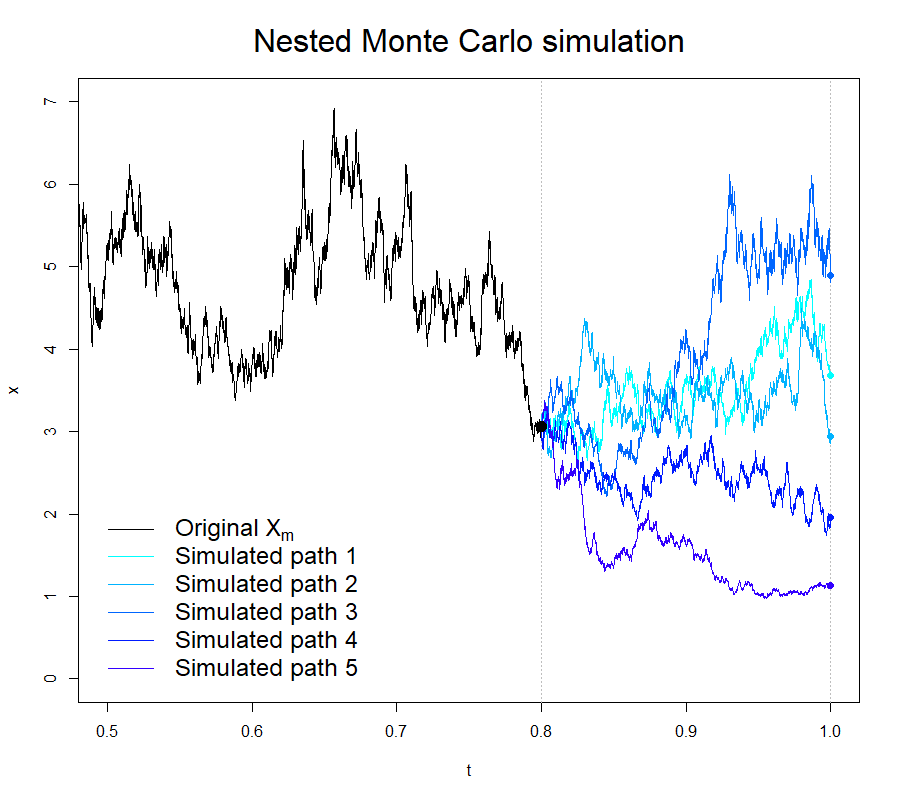
Figure 1: Nested Monte Carlo approach, $t_{k}=0.8$, $T=1$. Given the values $X_{m}(t_{k})$, $Y_{m}(t_{k})$, $U_{m,1}(t_{k})$, …, $U_{m,m}(t_{k})$, we simulate a number of trajectories $X^{(i)}_{m}$ on $(t_{k},T]$ (blue), use each of those to compute $F(X^{(i)}_{m}(T))(X^{(i)}_{m}(t_{k+1})-X^{(i)}_{m}(t_{k}))$ and $(X^{(i)}_{m}(t_{k+1})-X^{(i)}_{m}(t_{k}))^{2}$. The means of the latter values are then used as approximations of the required conditional expectations.

• given $X_{m}(t_{k})=x$, $Y_{m}(t_{k})=y$, $U_{m,1}(t_{k})=u_{1}$, …, $U_{m,m}(t_{k})=u_{m}$, simulate $N$ independent trajectories $\{X^{(i)}_{m}(t),~{}t\in(t_{k},T]\}$, $i=1,...,N$;

• for each trajectory, compute $F(X^{(i)}_{m}(T))(X^{(i)}_{m}(t_{k+1})-X^{(i)}_{m}(t_{k}))$ and $(X^{(i)}_{m}(t_{k+1})-X^{(i)}_{m}(t_{k}))^{2}$, $i=1,...,N$;

• put

  $$\widehat{\Phi}_{1}(t_{k},x,y,u_{1},...,u_{m}) :=\frac{1}{N}\sum_{i=1}^{N}F(X^{(i)}_{m}(T))(X^{(i)}_{m}(t_{k+1})-X^{(i)}_{m}(t_{k})),$$

  $$\widehat{\Phi}_{2}(t_{k},x,y,u_{1},...,u_{m}) :=\frac{1}{N}\sum_{i=1}^{N}(X^{(i)}_{m}(t_{k+1})-X^{(i)}_{m}(t_{k}))^{2}.$$

Example 5.1.

(Hölder continuous kernel) Consider the SVV model

$$X(t) =X(0)+\int_{0}^{t}Y(s)X(s)\left(\rho dB_{1}(s)+\sqrt{1-\rho^{2}}dB_{2}(s)\right),$$

$$Y(t) =Y(0)+\int_{0}^{t}b(s,Y(s))ds+\int_{0}^{t}\mathcal{K}(t,s)dB_{1}(s),$$

with $X(0)=5$, $Y(0)=1$, $\rho=0.5$, $b(t,y)=\frac{1}{(y-0.01)^{4}}-\frac{1}{(5-y)^{4}}$ and $\mathcal{K}(t,s)=\mathcal{K}(t-s)=(t-s)^{0.4}$. The approximation $(X_{m},Y_{m},U_{m,0},U_{m,1},...,U_{m,m})$ is constructed using the Bernstein polynomials as described in Subsection 4.3.

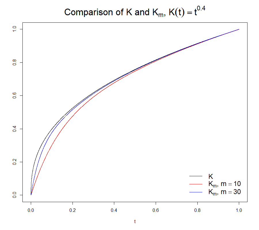
(a) Kernels $\mathcal{K}$ and $\mathcal{K}_{m}$

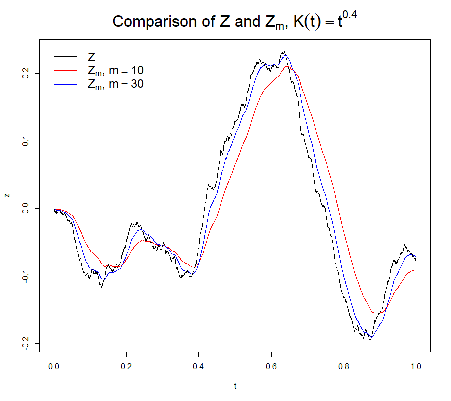
(b) Volterra noises $Z$ and $Z_{m}$

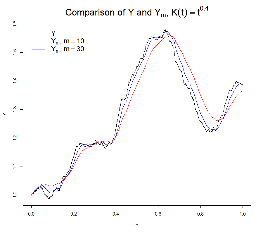
(c) Volatility processes $Y$ and $Y_{m}$

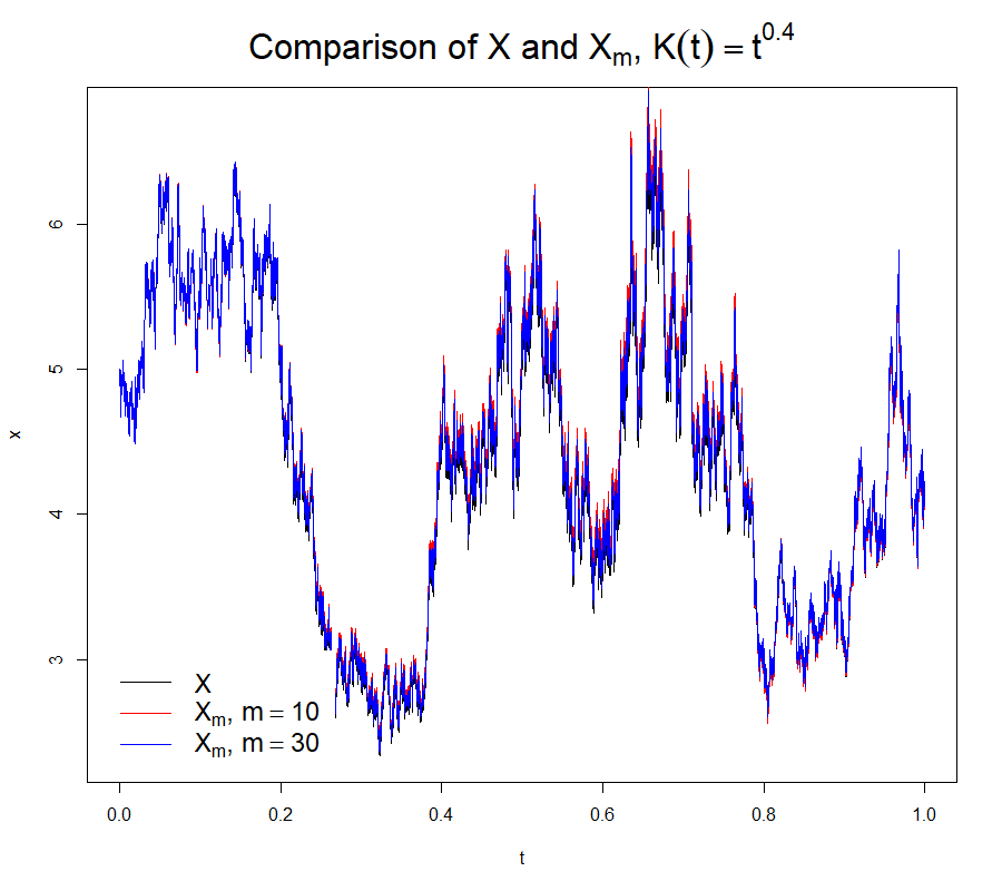
(d) Price processes $X$ and $X_{m}$

Figure 2: Approximation of the SVV model with Hölder continuous kernel

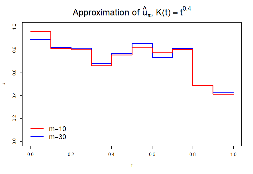
Figure 2 illustrates approximation of the SVV model; original kernel and generated sample paths of the corresponding processes are depicted in black whereas approximations using the Bernstein polynomials are depicted in red (of order $m=10$) and blue (of order $m=30$). Note that the path of $X$ simulated using the original noise (black) is not visible on Figure 2(d) due to the high degree of overlapping with the approximations (red and blue trajectories). Figure 3 contains a path of the process

$$\widehat{u}_{\pi}(t) :=\sum_{k=0}^{9}\frac{\widehat{\Phi}_{1}\left(\frac{k}{10},X_{m}\left(\frac{k}{10}\right),Y_{m}\left(\frac{k}{10}\right),U_{m,0}\left(\frac{k}{10}\right),...,U_{m,m}\left(\frac{k}{10}\right)\right)}{\widehat{\Phi}_{2}\left(\frac{k}{10},X_{m}\left(\frac{k}{10}\right),Y_{m}\left(\frac{k}{10}\right),U_{m,0}\left(\frac{k}{10}\right),...,U_{m,m}\left(\frac{k}{10}\right)\right)}\mathbbm{1}_{\left(\frac{k}{10},\frac{k+1}{10}\right]}(t),$$ (5.1)

with the European call payoff function $F(x):=\max\{x-4,0\}$ and the values $X_{m}\left(\frac{k}{10}\right)$, $Y_{m}\left(\frac{k}{10}\right)$, $U_{m,0}\left(\frac{k}{10}\right)$, …, $U_{m,m}\left(\frac{k}{10}\right)$ coming exactly from the trajectory depicted on Figure 2. In order to estimate

$$\widehat{\Phi}_{1}\left(\frac{k}{10},X_{m}\left(\frac{k}{10}\right),Y_{m}\left(\frac{k}{10}\right),U_{m,0}\left(\frac{k}{10}\right),...,U_{m,m}\left(\frac{k}{10}\right)\right),$$

$$\widehat{\Phi}_{2}\left(\frac{k}{10},X_{m}\left(\frac{k}{10}\right),Y_{m}\left(\frac{k}{10}\right),U_{m,0}\left(\frac{k}{10}\right),...,U_{m,m}\left(\frac{k}{10}\right)\right),$$

100000 simulations were used for each $k=0,1,...,9$.

Figure 3: Hedging strategy estimated for the path from Fig. 2 for $m=10$ (red) and $m=30$ (blue). The corresponding partition is $k/10$, $k=0,1,...,10$. Simulating the red line took 63231 seconds whereas the blue line – 73410 seconds.

Example 5.2.

(Rough kernel) Consider the SVV model

$$X(t) =X(0)+\int_{0}^{t}Y(s)X(s)\left(\rho dB_{1}(s)+\sqrt{1-\rho^{2}}dB_{2}(s)\right),$$

$$Y(t) =Y(0)+\int_{0}^{t}b(s,Y(s))ds+\int_{0}^{t}\mathcal{K}(t,s)dB_{1}(s),$$

with $X(0)=5$, $Y(0)=1$, $\rho=0.5$, $b(t,y)=\frac{1}{(y-0.01)^{4}}-\frac{1}{(5-y)^{4}}$ and $\mathcal{K}(t,s)=\mathcal{K}(t-s)=\frac{1}{\Gamma(0.8)(t-s)^{0.2}}$. The approximation $(X_{m},Y_{m},U_{m,1},...,U_{m,m})$ is constructed by approximating the Volterra noise $Z(t):=\frac{1}{\Gamma(0.8)}\int_{0}^{t}\frac{1}{(t-s)^{0.2}}dB_{1}(s)$ by a linear combination of standard Ornstein-Uhlenbeck processes as described in Subsection 4.2.

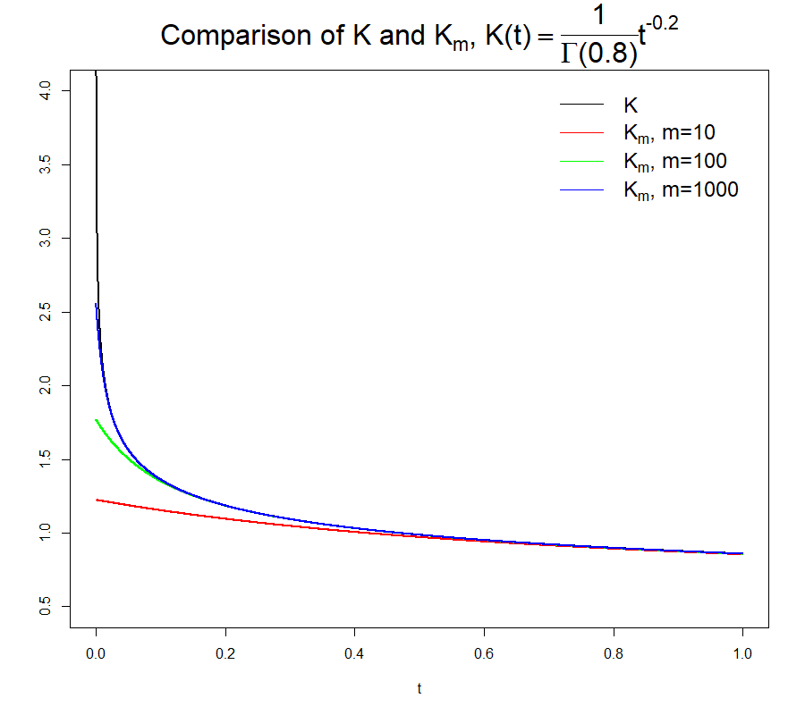
(a) Kernels $\mathcal{K}$ and $\mathcal{K}_{m}$

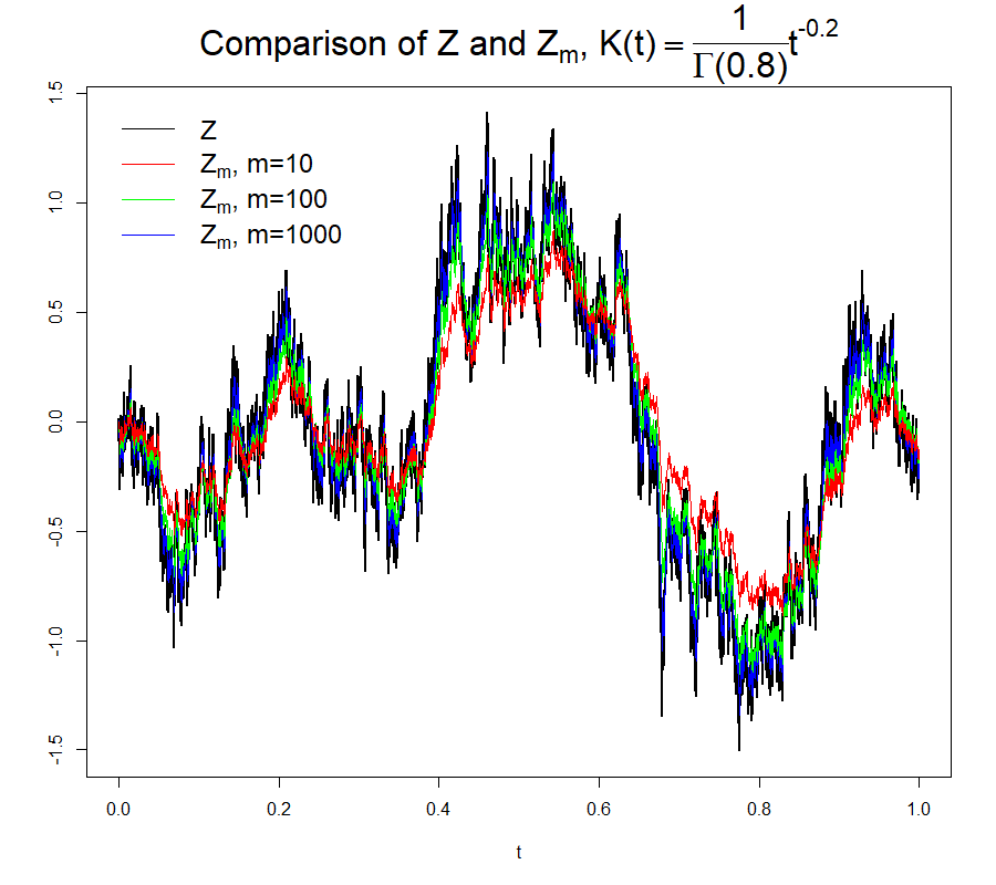
(b) Volterra noises $Z$ and $Z_{m}$

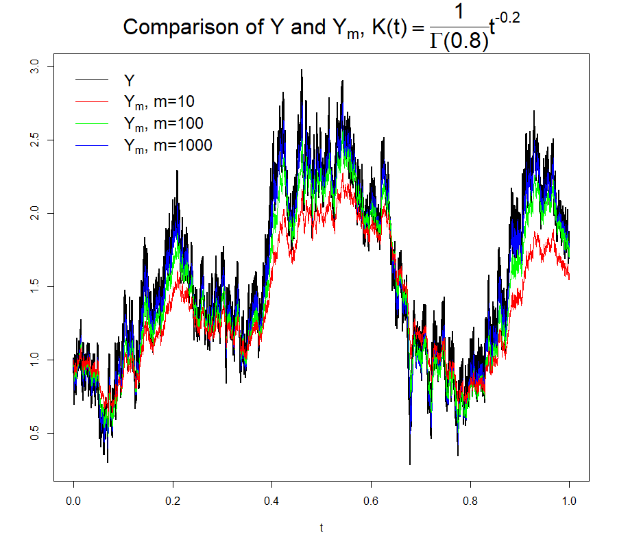
(c) Volatility processes $Y$ and $Y_{m}$

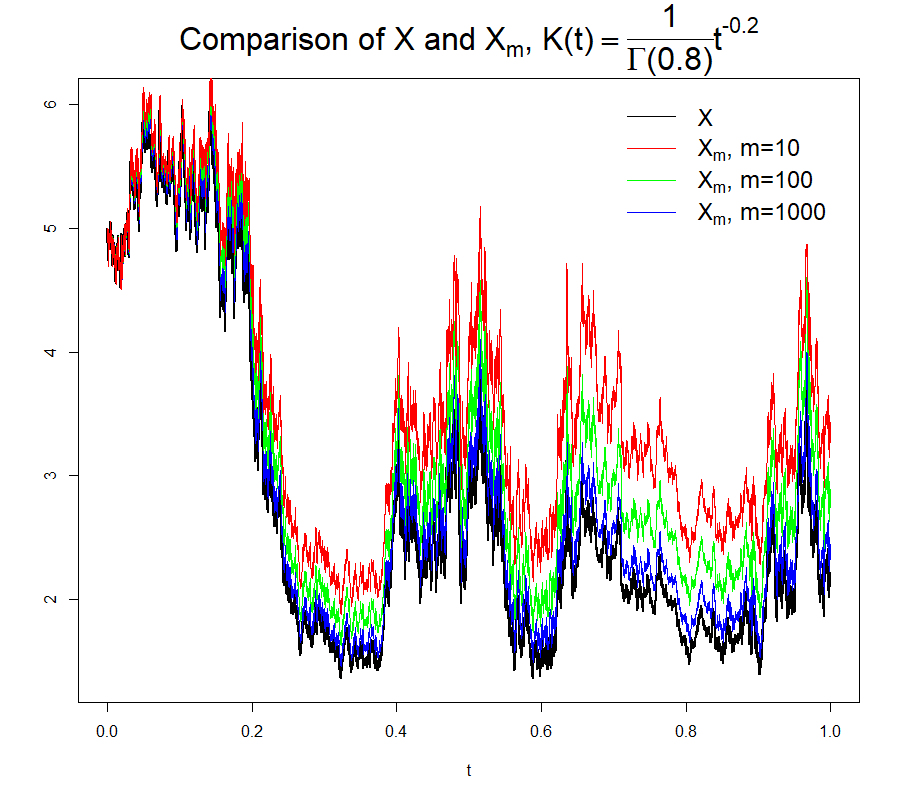
(d) Price processes $X$ and $X_{m}$

Figure 4: Approximation of the SVV model with rough fractional kernel

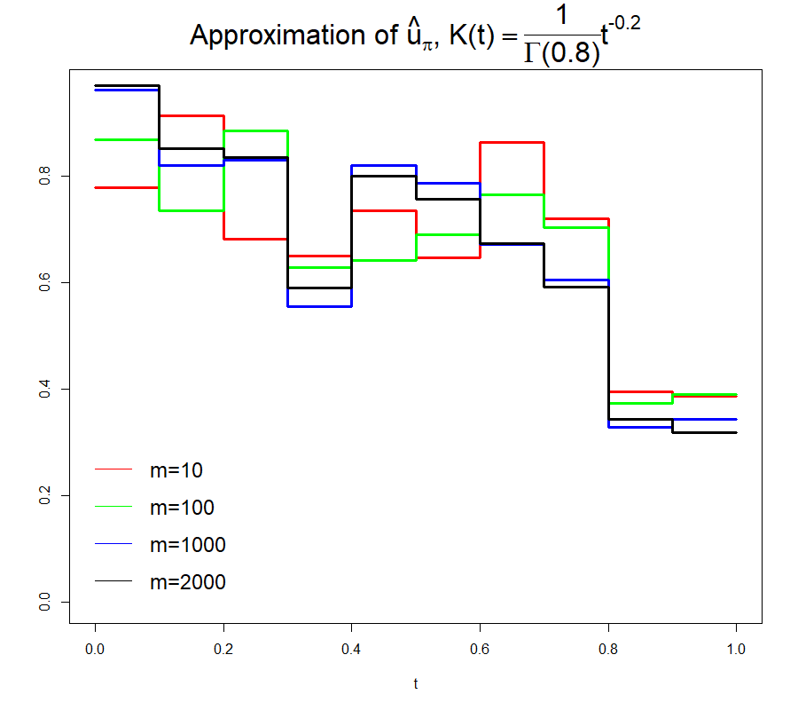
Just as in Example 5.1, Figure 4 illustrates approximation of the SVV model; original kernel and generated sample paths of the corresponding processes are depicted in black whereas approximations are depicted in red ($m=10$ summands), green ($m=100$ summands) and blue ($m=1000$ summands). Note that rough volatility requires much higher values of $m$ in order to ensure a decent level of approximation in comparison to Example 5.1.

Figure 5 contains a path of the process

$$\widehat{u}_{\pi}(t) :=\sum_{k=0}^{9}\frac{\widehat{\Phi}_{1}\left(\frac{k}{10},X_{m}\left(\frac{k}{10}\right),Y_{m}\left(\frac{k}{10}\right),U_{m,0}\left(\frac{k}{10}\right),...,U_{m,m}\left(\frac{k}{10}\right)\right)}{\widehat{\Phi}_{2}\left(\frac{k}{10},X_{m}\left(\frac{k}{10}\right),Y_{m}\left(\frac{k}{10}\right),U_{m,0}\left(\frac{k}{10}\right),...,U_{m,m}\left(\frac{k}{10}\right)\right)}\mathbbm{1}_{\left(\frac{k}{10},\frac{k+1}{10}\right]}(t),$$ (5.2)

$t\in[0,1]$, where the payoff function $F(x):=\max\{x-4,0\}$ and the values $X_{m}\left(\frac{k}{10}\right)$, $Y_{m}\left(\frac{k}{10}\right)$, $U_{m,1}\left(\frac{k}{10}\right)$, …, $U_{m,m}\left(\frac{k}{10}\right)$ are exactly the ones from the trajectory depicted on Figure 4. In order to estimate

$$\widehat{\Phi}_{1}\left(\frac{k}{10},X_{m}\left(\frac{k}{10}\right),Y_{m}\left(\frac{k}{10}\right),U_{m,0}\left(\frac{k}{10}\right),...,U_{m,m}\left(\frac{k}{10}\right)\right),$$

$$\widehat{\Phi}_{2}\left(\frac{k}{10},X_{m}\left(\frac{k}{10}\right),Y_{m}\left(\frac{k}{10}\right),U_{m,0}\left(\frac{k}{10}\right),...,U_{m,m}\left(\frac{k}{10}\right)\right),$$

100000 simulations were used for each $k=0,1,...,9$.

Figure 5: Hedging strategy estimated for the path from Fig. 4 for $m=10$ (red), $m=100$ (green), $m=1000$ (blue) and $m=2000$ (black). The corresponding partition is $k/10$, $k=0,1,...,10$. The figure also illustrates slower rate of convergence in comparison to the Hölder kernel case: the black and blue lines are close to each other but the red and green lines (corresponding to relatively low values of $m$) differ substantially. Computation time: 24162 seconds for $m=10$, 25348 seconds for $m=100$, 38530 seconds for $m=1000$ and 42431 seconds for $m=2000$.

5.2 Least squares Monte Carlo method

Despite its simplicity and clear theoretical justification, the nested Monte Carlo approach has a substantial disadvantage: it takes long to compute and thus requires powerful computational resources in order to be used in practice. In order to overcome this issue, one can use the Least Squares Monte Carlo (LSMC) method instead:

• simulate $N$ independent realizations

  $$(X^{(i)}_{m},Y^{(i)}_{m},U^{(i)}_{m,1},...,U^{(i)}_{m,m})=\left\{\big{(}X^{(i)}_{m}(t),Y^{(i)}_{m}(t),U^{(i)}_{m,1}(t),...,U^{(i)}_{m,m}(t)\big{)},~{}t\in[0,T]\right\},$$

  $i=1,...,N$;

• for each path, evaluate

  $$\big{(}X^{(i)}_{m}(t_{k}),Y^{(i)}_{m}(t_{k}),U^{(i)}_{m,1}(t_{k}),...,U^{(i)}_{m,m}(t_{k})\big{)},$$

  $$F(X^{(i)}_{m}(T))(X^{(i)}_{m}(t_{k+1})-X^{(i)}_{m}(t_{k}))$$

  and

  $$(X^{(i)}_{m}(t_{k+1})-X^{(i)}_{m}(t_{k}))^{2},$$

  $i=1,...,N$;

• apply an appropriate non-parametric regression (with a mean squared error loss function) to the generated “dataset” treating

  $$\big{(}X^{(i)}_{m}(t_{k}),Y^{(i)}_{m}(t_{k}),U^{(i)}_{m,1}(t_{k}),...,U^{(i)}_{m,m}(t_{k})\big{)},\quad i=1,...,N,$$

  as “input” and

  $$F(X^{(i)}_{m}(T))(X^{(i)}_{m}(t_{k+1})-X^{(i)}_{m}(t_{k})),\quad(X^{(i)}_{m}(t_{k+1})-X^{(i)}_{m}(t_{k}))^{2},\quad i=1,...,N,$$

  as “output” variables. The resulting estimates $\widehat{\Phi}_{1}(t_{k},\cdot)$, $\widehat{\Phi}_{2}(t_{k},\cdot)$ of the regression functions are then used to calculate $\widehat{u}_{\pi}$ on the interval $(t_{k},t_{k+1}]$.

Remark 5.3.

The Least Squares Monte Carlo method described above can be regarded as a simplified version of the approach suggested in [11, 33, 38] for pricing American options or in [30, 31, 32] for modeling of life insurance companies.

Example 5.4.

Fig. 6 contains approximations of the optimal hedging strategy constructed for the path of $X_{m}$ from Example 5.1 that corresponds to $m=10$. In order to obtain the dark green line, we simulated the “dataset” containing the “input” variables

$$\big{(}X^{(i)}_{m}(t_{k}),Y^{(i)}_{m}(t_{k}),U^{(i)}_{m,0}(t_{k}),...,U^{(i)}_{m,m}(t_{k})\big{)},\quad i=1,...,N,$$

together with the corresponding “output” variables

$$F(X^{(i)}_{m}(T))(X^{(i)}_{m}(t_{k+1})-X^{(i)}_{m}(t_{k})),\quad(X^{(i)}_{m}(t_{k+1})-X^{(i)}_{m}(t_{k}))^{2},\quad i=1,...,N,$$

with $N=1000000$ for each $k=0,1,...,9$. In order to compute $\widehat{\Phi}_{1}(t_{k},\cdot)$, $\widehat{\Phi}_{2}(t_{k},\cdot)$, we used the idea from [31] and utilized a neural network with 3 hidden layers and 20 nods in each layer. The red line is exactly the path of $\hat{u}_{\pi}$ for $m=10$ from Fig. 3 and is treated as a reference.

Figure 6: Approximation of the optimal hedge using the Nested Monte Carlo method for $m=10$ from Fig. 3 (red) and using the Least Squares Monte Carlo method (dark green).

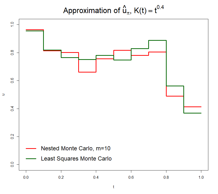
Note that the Nested approach described in Example 5.1 required 63231 seconds to simulate a path of $\hat{u}_{\pi}$ corresponding to a single realization of $(X_{m},Y_{m},U_{m,0},...U_{m,m})$ whereas the Least Squares modification took roughly 6 days to simulate the initial dataset and about 5 hours to fit the neural network. Once ready, the actual computations were conducted almost instantly.

Remark 5.5.

The neural network architecture in Example 5.4 is not optimal. It is fairly clear from Fig. 6: even though the LSMC Monte Carlo estimate preserves in general the shape of the reference optimal hedge simulated using the NMC approach, the difference between the two is still quite substantial. We emphasize that performance of the NMC method heavily depends on the chosen non-parametric regression method, and therefore a separate investigation on performance of different regression approaches is required.

Remark 5.6.

Similar method can theoretically be applied for the SVV model with a rough fractional kernel. However, as noted in Example 5.2, one may need a very high dimensionality of the “input” variables vector (over 1000) which requires a dataset with possibly unrealistically huge number of observations.

References

- [1] Abi Jaber, E., and El Euch, O. Multifactor approximation of rough volatility models. SIAM journal on financial mathematics 10, 2 (2019), 309–349.
- [2] Abi Jaber, E., Miller, E., and Pham, H. Linear-quadratic control for a class of stochastic Volterra equations: Solvability and approximation. The annals of applied probability 31, 5 (2021).
- [3] Alòs, E., and Garcia Lorite, D. Malliavin calculus in finance: Theory and practice. CRC Press, London, England, 2021.
- [4] Alòs, E., León, J. A., and Vives, J. On the short-time behavior of the implied volatility for jump-diffusion models with stochastic volatility. Finance and stochastics 11, 4 (2007), 571–589.
- [5] Andersen, L. B. G., and Piterbarg, V. V. Moment explosions in stochastic volatility models. Finance Stoch. 11, 1 (2007), 29–50.
- [6] Avikainen, R. On irregular functionals of SDEs and the Euler scheme. Finance and stochastics 13, 3 (2009), 381–401.
- [7] Azmoodeh, E., Sottinen, T., Viitasaari, L., and Yazigi, A. Necessary and sufficient conditions for Hölder continuity of Gaussian processes. Statistics & Probability Letters 94 (2014), 230 – 235.
- [8] Bayer, C., Friz, P., and Gatheral, J. Pricing under rough volatility. Quantitative finance 16, 6 (2016), 887–904.
- [9] Bäuerle, N., and Desmettre, S. Portfolio optimization in fractional and rough Heston models. SIAM journal on financial mathematics 11, 1 (2020), 240–273.
- [10] Carmona, P., and Coutin, L. Fractional Brownian motion and the Markov property. Electronic communications in probability 3 (1998), 95–107.
- [11] Carriere, J. F. Valuation of the early-exercise price for options using simulations and nonparametric regression. Insurance, mathematics & economics 19, 1 (1996), 19–30.
- [12] Chronopoulou, A., and Viens, F. G. Estimation and pricing under long-memory stochastic volatility. Annals of finance 8, 2–3 (2012), 379–403.
- [13] Comte, F., Coutin, L., and Renault, E. Affine fractional stochastic volatility models. Annals of finance 8, 2–3 (2012), 337–378.
- [14] Comte, F., and Renault, E. Long memory in continuous-time stochastic volatility models. Mathematical Finance 8, 4 (1998), 291–323.
- [15] Cont, R. Long range dependence in financial markets. In Fractals in Engineering. Springer-Verlag, 2005, p. 159–179.
- [16] Cont, R. Volatility clustering in financial markets: Empirical facts and agent-based models. In Long Memory in Economics. Springer Berlin Heidelberg, 2006, p. 289–309.
- [17] Di Nunno, G. Stochastic integral representations, stochastic derivatives and minimal variance hedging. Stoch. Stoch. Rep. 73, 1-2 (2002), 181–198.
- [18] Di Nunno, G., Mishura, Y., and Yurchenko-Tytarenko, A. Drift-implicit Euler scheme for sandwiched processes driven by Hölder noises. To appear in Numerical Algorithms (2022).
- [19] Di Nunno, G., Mishura, Y., and Yurchenko-Tytarenko, A. Option pricing in Volterra Sandwiched Volatility model. arXiv:2209.10688 [q-fin.MF] (2022).
- [20] Di Nunno, G., Mishura, Y., and Yurchenko-Tytarenko, A. Sandwiched SDEs with unbounded drift driven by Hölder noises. To appear in Advances in Applied Probability 55 (2023).
- [21] Di Nunno, G., Øksendal, B., and Proske, F. Malliavin calculus for Lévy processes with applications to finance. Springer, Berlin, Heidelberg, 2009.
- [22] El Euch, O., and Rosenbaum, M. The characteristic function of rough Heston models. Mathematical Finance. An International Journal of Mathematics, Statistcs and Financial Economics 29, 1 (2019), 3–38.
- [23] Fukasawa, M. Asymptotic analysis for stochastic volatility: martingale expansion. Finance and stochastics 15, 4 (2011), 635–654.
- [24] Fukasawa, M. Volatility has to be rough. Quantitative finance 21, 1 (2021), 1–8.
- [25] Fukasawa, M., and Gatheral, J. A rough SABR formula. Frontiers of Mathematical Finance 1, 1 (2022), 81.
- [26] Funahashi, H., and Kijima, M. A solution to the time-scale fractional puzzle in the implied volatility. Fractal and fractional 1, 1 (2017), 14.
- [27] Garsia, A., Rodemich, E., and Rumsey, H. A real variable lemma and the continuity of paths of some Gaussian processes. Indiana Univ. Math. J. 20 (1970), 565–578.
- [28] Gatheral, J., Jaisson, T., and Rosenbaum, M. Volatility is rough. Quantitative finance 18, 6 (2018), 933–949.
- [29] Harms, P., and Stefanovits, D. Affine representations of fractional processes with applications in mathematical finance. Stochastic processes and their applications 129, 4 (2019), 1185–1228.
- [30] Krah, A.-S., Nikolić, Z., and Korn, R. A least-squares Monte Carlo framework in proxy modeling of life insurance companies. Risks 6, 2 (2018), 62.
- [31] Krah, A.-S., Nikolić, Z., and Korn, R. Least-squares Monte Carlo for proxy modeling in life insurance: Neural networks. Risks 8, 4 (2020), 116.
- [32] Krah, A.-S., Nikolić, Z., and Korn, R. Machine learning in least-squares Monte Carlo proxy modeling of life insurance companies. Risks 8, 1 (2020), 21.
- [33] Longstaff, F. A., and Schwartz, E. S. Valuing american options by simulation: A simple least-squares approach. The review of financial studies 14, 1 (2001), 113–147.
- [34] Mathé, P. Approximation of Hölder continuous functions by Bernstein polynomials. The American mathematical monthly: the official journal of the Mathematical Association of America 106, 6 (1999), 568–574.
- [35] Nualart, D. The Malliavin calculus and related topics, 2 ed. Springer, Berlin, Germany, 2006.
- [36] Pham, H. On quadratic hedging in continuous time. Mathematical methods of operations research 51, 2 (2000), 315–339.
- [37] Schweizer, M. A guided tour through quadratic hedging approaches. In Handbooks in Mathematical Finance: Option Pricing, Interest Rates and Risk Management, E. Jouini, J. Cvitanic, and Musiela, Eds. Cambridge University Press, 2001, p. 538–574.
- [38] Tsitsiklis, J. N., and Van Roy, B. Regression methods for pricing complex American-style options. IEEE transactions on neural networks 12, 4 (2001), 694–703.
- [39] Wang, R., and Xiao, Y. Exact uniform modulus of continuity and Chung’s LIL for the generalized fractional Brownian motion. Journal of theoretical probability (2022).
- [40] Zhu, Q., Loeper, G., Chen, W., and Langrené, N. Markovian approximation of the rough Bergomi model for Monte Carlo option pricing. Mathematics 9, 5 (2021), 528.