Iterating sum of power divisor function and New equivalence to the Riemann hypothesis

Abstract

Mathematicians have been interested in the problem of grasping odd perfect numbers and multiperfect numbers for more than one millennium and it is not known whether or not odd perfect numbers can exist. However it is known that there is no such number below $10^{300}$ Moreover it has been proved by Hagis and Chein independently that an odd perfect number must have at least $8$ prime factors. In fact results of this latter type can in principle be obtained solely by calculation, in view of the result of Pomerance who showed that if $N$ is an odd perfect number with at most $k$ prime factors, then

$$N\leq{{(4k)^{(4k)}}^{2}}^{k^{2}}$$

it is a long-standing open question whether an odd perfect $N$ number exists , several authors gave necessary conditions for the existence of an odd perfect number using advanced techniques and theories in analytic number theory which uses arithmetic sequences like sum divisor function and Euler totionent function also Aliquot sequence ,One may ask what is the fast way among these techniques to get an odd perfect number ? however, we can’t give an affirmative answer to this question but we may give an acceptable answer , namely, thinking about iterative of sum power divisor function which it is the aim of this paper and we wouldn’t investigate about existence of odd perfect number just we may investigate the behavior of iterative sum power divisor function and its periodicity .

Inspired by the question of Graeme L. Cohen and Herman J. J. te Riele , The Authors of [4] who they investigated a question :Given $m$ is there an integer $k$ for which $\sigma^{k}(m)=0\bmod m$? They did this in a $1995$ paper and asserted through computation that the answer was yes for $m\leq 400$,We were able in this paper to give a negative answer to the reverse question of Graeme L. Cohen and Herman J. J. te Riele such that we showed that there is no fixed integer $m$ for which $\sigma^{k}(m)=0\bmod m$ for all iterations $k$ of sum divisor function using H.Lenstra problem result for Aliquot sequence and we showed that there exists some integers $m$ such that $\sigma_{k}(m)\bmod m$ is periodic with small period $L=2$(periodicity with small period dividing $L$ the lcm the least common multiple of $1$+each exponents in the prime factorization of $m$ ).A new equivalence to the Riemann hypothesis has been added using congruence and divisibility among sum of power divisor function where some numerical evidence in the stochastic and statistics context are presented such we were able to derive new fit distribution model from the behavior of the sequence $\sigma_{k}(m)\bmod m$

Keywords Iterative sum power divisor function  $\cdot$ Aliquot sequence  $\cdot$ Squarefree integers  $\cdot$ periodic sequences

1 Introduction

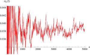
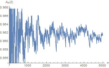
Early mathematicians were particularly interested in perfect numbers, defined as numbers where $s(n)=n$. The first few perfect numbers are $6,28,496$ and $8128$; Around $300$ B.C., Euclid showed showed that if $2^{p-1}-1$ is prime, then $2^{p-1}(2^{p}-1)$ is perfect [1]. However, it took another two millennia for Euler to show that all even perfect numbers are of the form discovered by Euclid [2]. It is not known if there are any odd perfect numbers, but if they do exist, then they must be greater than $101500$ [3]. Numbers where $s(n)<n$ are known as deficient, whilst those where $s(n)>n$ are abundant. Deficient numbers (density function) is shown in Figure (2) with blue plot points, whilst abundant numbers is shown in figure (1) above it with red plot points. Deficient numbers appear to be more common than abundant numbers.

Figure 1: Density function for abundant numbers

Figure 2: Density function for deficient numbers

In all of this paper $s(m)=\sigma(m)-m$ denote the sum of propre divisor function ,namely ,Aliquot sequence and $s^{0}(m)=m,s^{k}(m)=s(s^{k-1}))$ the iteration of Aliquot sequence ,We define $\sigma$ is sum of divisor function such that:$\sigma^{0}(m)=m,\sigma^{k}(m)=\sigma(\sigma^{k-1}(m)),m\geq 1$ the iterated of sum of divisor function and $\sigma_{k}{(n)}=\sum_{d\mid n}d^{k}$ the sum of divisors function of the $k$ th power, where $k\in\mathbb{N_{0}}$

There is a great deal of literature concerning the iteration of the function $s(m)=\sigma(m)-m$ , much of it concerned with whether the iterated values eventually terminate at zero, cycle or become unbounded depending on the value of $m$ see [5] and see ([6],p.64 ) ,[31] ,for details ,Less work has been done on $\sigma$ iterate itself.Many problems on iterate of sum divisor function remain open ,proving or disproving them using numerical evidence are beyond of current technology .Some of these open problems are :

• 1) for any $n>1$,$\frac{\sigma^{m+1}(n)}{\sigma(m)}\to 1$ as , $m\to\infty$

• 2) for any $n>1$,$\frac{\sigma^{m+1}(n)}{\sigma^{m}(n)}\to\infty$ as , $m\to\infty$

• 3) for any $n>1$,$\sigma^{1/m}(n)\to\infty$ as $m\to\infty$

• 4) for any $n>1$,there is $m$ with $n|\sigma^{m}(n)$

• 5) for any $n,l>1$,there is $m$ with $l|\sigma^{m}(n)$

• 6) for any $n_{1},n_{2}>1$ , there are $m_{1},m_{2}$ with : $\sigma^{m_{1}}(n_{1})=\sigma^{m_{1}}(n_{2})$

• 7)Is $\liminf\frac{\sigma_{k}(n)}{n}$ finite for every $k$ ?

  We can neither prove nor disprove any of these statements, for more details about these statments see [5, 8] and see ([7],p.169)

2 Main results

• 1) There is no integer $m$ for which $\sigma^{k}(m)=0\bmod m$ , for all iterations $k$ ,with $\sigma^{k}(m)$ is the $k$-fold iterate of $\sigma$ the sum divisor function

• 2) If $m$ is multiperfect number with $L$ the lcm of $1$+ each exponents in the prime factorisation of $m$ , and with $L$ prime then $m=6$

• 3) Riemann hypothesis is false if and only if there exist a pair of positive integers $(m,k)$ such that $\sigma_{k}(m)\bmod m$ is not periodic in $k$

2.1 Proof of result 1

Firstly,The congruence $\sigma(m)=0\bmod m$ means $m$ is a multiply perfect number. To avoid trivialities we assume $m>1$. Note that $\frac{\sigma(m)}{m}$ is bounded above by the product over all primes $q$ dividing $m$ of $\frac{q}{q-1}$, which is $\mathcal{O}(\log p)$ with $p$ the largest prime divisor of $m$, and strictly less than $p$ when $p>3$. (Indeed, it is less than $\omega(m)$, the number of distinct prime divisors of $m$, when $\omega(m)>4$.) While $\sigma(m)$ itself does not have to be multiperfect, We suspect there are finitely many numbers with $\sigma(\sigma(m))$ a multiple of $m$. In particular, let $g_{0}=m_{0}=m$, $m_{n+1}=\sigma(m_{n})$, and $g_{n+1}=\gcd(g_{n},m_{n+1})$. We suspect $g_{3}<m$. We base this suspicion on the observation that the power of $2$ exactly dividing $m_{n}$ appears to change between $m_{n},m_{n+1}$, and $m_{n+2}$.

Let us write $w$ for $\omega(m)$ and let us note that for a multiperfect $m$, $m_{1}$ will differ from $m$ by having less than $\mathcal{O}(\log(w))$ additional prime factors, some in common with the prime factors of $m$. So the prime factorization of $m_{1}$ looks very much like the prime factorization of $m$.

We would like to argue that the prime factorization of $m_{2}$ should be quite different from that of $m_{1}$, because any additional powers of $q$ for $q$ a small prime dividing $n$ will affect $\sigma(q^{n})$ and thus remove some prime factors. However, it is possible that there are (insanely large) odd multiperfect numbers which would be factors of $m$ and not be affected by this. Indeed, this question may be equivalent to the question of the existence of large odd multiperfect numbers.

Let us look at $S(m)=\frac{\sigma(m)}{m}$. Letting the following products run over the distinct primes $q$ dividing $m$, we have $\prod\frac{q+1}{q}<S(m)<\prod\frac{q}{q-1}$. (And the lower bound is at least half the upper bound, so we have $S(m)\simeq\prod\frac{q}{q-1}$.) As observed above, $S(m)<\omega(m)$ when $4<\omega(m)$ and $S(m)<2\omega(m)$ the rest of the time. So $S(m)$ is pretty small compared to $m$ and often small compared to $\log p$ where $p$ is the greatest prime factor of $m$.

Let $r_{n}=m_{n+1}/m_{n}=S(m_{n})$. The assumption in the problem implies $r_{n}>r_{0}$, for if $m$ properly divides $k$ then $S(m)<S(k)$. Then $m_{n}>mr_{0}^{n}$ for all $n$, since $m_{n}$ is an increasing sequence. We believe we can’t have both conditions hold indefinitely. However, We now switch ground on our assertion above that $g_{3}<m$ always happens: We think it can, We just don’t think we will see an example with fewer than a 1000 decimal digits (which isn’t insanely large).

Here is two examples ,probably they encourage us to think that we have high chance to have metaperfect number for all iteration $k$, The number $m=13188979363639752997731839211623940096$ satisfies $\sigma(m)=5m$ and since $\gcd(5,m)=1$ $\sigma^{2}(m)=\sigma(5m)=6\sigma(m)=30m$,so at least there’s one example where $m_{1}$ and $m_{2}$ are multiples of $m$. Whether $m$ qualifies as very large indeed is a matter of taste,Another example $\sigma^{32}(2)=564210119465811\equiv 1\bmod 2$ we don’t think so if it has been proved that $\sigma^{k}(2)\equiv 0\bmod 2$ for all $k\geq 33$, One can check the data in this sequence at OEIS :http://oeis.org/A007497/b007497.txt .

Now , When $S(m)$ is coprime to $m$, we clearly have $m\mid m_{2}$ as well as $m\mid m_{1}$, and by multiplicativity of $S$ we also have $S(S(m)m)=S(S(m))S(m)$. What if $S(m)$ is not coprime to $m$? We still have

$$S(S(m)m)<S(m)S(S(m)).$$ (1)

This last is the crux. $S()$ grows slower than $\log()$, so we need to show this contradicts the growth rate implied by all $m_{n}$ being multiples of $m$. We may rewrite the last inequality (1) in the context of Lenstra sharper result ,Lenstra proved in [11, 9] that for every $k$ there is an $m$ so that ($s^{1}(m)$) will for simplicity be denoted by $s(m))$ :

$$s^{0}(m)<s(m)<s^{2}(m)<\cdots<s^{k}(m)$$ (2)

The sharper result were derived from Lenstra result ,namely inequality (2) is reformulated as a Theorem in,see Theorem1 in ([10],p.642) which states :

Theorem1: For every $k$ and $\delta>0$ and for all $m$ except a sequence of density $0$

$$(1-\delta)m\bigg{(}\frac{s(m)}{m}\bigg{)}^{i}<s^{i}(m)<(1+\delta)m\bigg{(}\frac{s(m)}{m}\bigg{)}^{i},1\leq i\leq k$$ (3)

We shall show that the right hand side of inequality (1) behave like the upper bound of $s^{i}(m)$ in (3) , (1) can be rewritten as:

$$\frac{\sigma(\sigma(m))}{\sigma(m)}<\sigma\bigg{(}\frac{\sigma(m)}{m}\bigg{)}$$ (4)

With the assumption that $m$ is not coprime to $S(m)=\frac{\sigma(m)}{m}$ means that $S(m)$ must be an integer thus $m|S(m)$ in the same time $m|\sigma(m)$ ,thus $m$ is metaperfect number for the first iteration ,let $d$ be the largest prime divisor of $\sigma(m)$ and since $m|\sigma(m)$ the inequality which is defined in (4) becomes :

$$\frac{\sigma(\sigma(m))}{\sigma(m)}<\sigma\bigg{(}\frac{\sigma(m)}{m}\bigg{)}=\sigma(d)\leq d\bigg{(}\frac{d}{d-1}\bigg{)}^{\omega(d)}$$ (5)

Here $\omega(d)$ denote the number of divisor of $d$ which is $1$ in this case since $d$ is assumed to be a prime number , Finally we can come up to the final inequality using (5) such that

$$\frac{\sigma(\sigma(m))}{\sigma(m)}<\sigma(d)\leq d\bigg{(}1+\frac{1}{d-1}\bigg{)}^{\omega(d)}$$ (6)

let $\delta=\frac{1}{d-1},s(m)=\sigma(m)-m$ and the symbole of iteration $i$ must be denote $\omega(d)$, yield to have (5) hold.

The same steps would work in the case of $d$ is not a prime divisor .We may let this case as a short exercise for readers.We have showed in the case of $S(m)$ is not coprime to $m$ that we have the similar inequality with the inequality defined in Theorem1 ,namely,The sharper result which it were proved by H Lenstra ,thus we have always the same upper bound as given in (3) ,thus lead to the proof of the first result rather than that there is no integer $m$ satisfies the congruence $\sigma^{k}(m)=0\bmod m$, for all iteration $k$ .

A weak affirmation to show that we still have inequality (1) hold is Robin’s criterion [12], In [12] ,Theorem 1.3, (page 358) states the following by the assumption of RH to be true

Theorem2: The RH is true if and only if for all even non-squarefree integers $m\geq 5044$ Robin’s inequality

$$\sigma(m)<e^{\gamma}m\log\log m$$ (7)

is satisfied.The inequality defined in (7) means that for all $n>5040,S(m)=\frac{\sigma(m)}{m}$ can’t grow too fast,And Robin also proved in [13] that :

$$\ \sigma(n)<e^{\gamma}n\log\log n+\frac{0.6483\ n}{\log\log n},n\geq 3$$ (8)

both of inequalities (7) and (8) show to us that (1) still hold for some even non square free integers .

2.2 Proof of result 2

Key idea:

The key idea in showing $m=6$ is the only multiperfect number with $L$ prime is to show all prime factors of $\sigma(m)$ and thus of $m$ are $0$ or $1\bmod L$ all with multiplicity $L-1$ and thus $\bigg{(}\frac{L}{(L-1)}\bigg{)}^{n+1}\geq\frac{\sigma(m)}{m}\geq L$ where $n$ is the number of distinct prime factors of $m$ that are $1\bmod L$. This quickly leads to $L=2$, and then showing the largest prime factor of $m$ must be at most one more than the second largest prime factor.

Proof: Note that if $L$ is prime, then the prime factors of$m$ all occur with the same multiplicity, namely $L-1$. Thus $\sigma(m)$ is a product of terms of the form $\sigma(p^{L-1})$, which means (since $L$ is prime) that each factor of $\sigma(p^{L-1})$ is either $L$ or is a prime which is $1\bmod L$. This means $m$ and $\sigma(m)$ both have as prime factors only numbers $q$ which are either$0$ or $1\bmod L$. If $L$ is a factor of $m$, then it occurs to the Lth power, by hypothesis. If $q=kL+1$ is a factor of $m$, then $\sigma(q^{L-1})$ is divisible by $L$ exactly once, using standard elementary results. Thus $\sigma(m)$ is divisible by $L^{n}$ or by $L^{n+L}$ exactly,where $n$ counts the number of distinct prime factors of $m$ that are $1\bmod L$.

Suppose $m$ is at least as large as $L$. Then $\frac{\sigma(m)}{m}$ is at least $L^{m}/L^{L-1}$, but also $\frac{\sigma(m)}{m}$ is less than $(L/(L-1))^{m+1}$, by standard inequalities for $\sigma()$. Taking logs, we have $(m+1-L)\log L$ is less than or equal to $\frac{\sigma(m)}{m}$ which is less than $(m+1)/(L-1)$, or $\log L$ is less than $(1+\frac{L}{(m+1-L))(L-1)})$ which is at most $3$ when $L$ is $2$ , is at most $2$ when$L$ is $3$, and is at most $1.5$ when $L$ is $5$ or larger. The only solutions to the inequality with $L$ a prime are$L=3$ and $m$ at most $4$, and $L=2$.

If $m$ is smaller than $L$, then we have $\frac{\sigma(m)}{m}$ is no more than $\bigg{(}\frac{L}{(L-1)}\bigg{)}$ which is at most $4$. But $\frac{\sigma(m)}{m}$ is at least $L$, since all prime factors of $\sigma(m)$ are $0$ or $1\bmod L$, so again $L$ is $2$ or $3$.

If $L$ is $3$, we now are faced with $3$ less than or equal $\frac{\sigma(m)}{m}$ less than $(3/2)(7/6)^{m}$ for $m$ at most $4$, since we have to take the primes which are $1\bmod 3$ into account. But $(7/6)^{4}$ is less than $2$. So $L$ cannot be $3$

So if $m$ is multiperfect and $L$ is prime, then $L$ must be $2$, and thus $m$ is squarefree. It is now easy to show $m$ must be $6$, for instance by considering the largest prime factor of $m$ has to be at most one more than the second largest prime factor of $m$.We leave this as exercice for readers .

Another hard method to show that $6$ is the only multiperfect number which satisfies periodicity in $k$ with small prime period $L=2$ using divisibility and congruence among sum power divisor function . for starting point let $r=\gcd(k,e+1)$, and $p$ a prime. Then $\sigma_{k}(p^{e})\equiv r\frac{p^{e+1}-1}{p^{r}-1}\bmod\sigma(p^{e})$. Also, $r=1$ if and only if $\sigma(p^{e})$ divides $\sigma_{k}(p^{e})$. Thus for $k$ coprime to $\tau(m)$, we have $\sigma(m)$ divides $\sigma_{k}(m)$. The relation also suggests that for a given $m$ the sequence $\sigma_{k}(n)\bmod\sigma(n)$ is periodic in $k$ with a period dividing $L$, the least common multiple of ($1+$ each exponent) in the prime factorization of $m$. Once can show a nonreduced representation $\sigma_{k}(m)=a_{k}\sigma(m)/b_{k}$ where the $b_{k}$ are integers not necessarily coprime to the integers $a_{k}$ or to $a_{k}\sigma(m)$, with the property that the $b_{k}$ are bounded and periodic with period $L$. This is not enough to show $\sigma_{k}(m)\bmod\sigma(m)$ is periodic with small period, unfortunately.

If now $m$ is multiperfect (so $m$ divides $\sigma(m)$) we have $m$ divides $\sigma_{k}(m)$ for $k$ coprime to $\tau(m)$. In particular if $\tau(m)$ is a power of $2$, then $m$ divides $\sigma_{k}(m)$ for all odd $k>0$.

It is still possible that $m$ can divide $\sigma_{k}(m)$ for $k$ not coprime to $\tau(m)$. However if $L$ is not prime, it seems likely that there will be more than one nonzero value of $\sigma_{k}(m)\bmod\sigma(m)$. If this is so, it would be one ingredient in a proof that $6$ is the unique number having the claimed properties in result2, the other ingredient being that $6$ is the only nontrivial multiperfect number with $L$ a prime.

We have noted some flaws in our analysis about claiming that $6$ is the only integer satisfies periodicity with small period $L=2$, one expects multiperfect numbers other than $1$ and $6$ to be a multiple of $4$; when $m$ satisfies $\sigma(m)\bmod m=0$ and $\sigma_{2}(m)\bmod m=2$, and in addition $m\bmod 4=0$, then all odd prime factors of $m$ except one must occur to an even multiplicity, and the remaining odd prime factor must occur to a multiplicity of $1\bmod 4$ and must be a prime that is $3\bmod 4$. While simple, these observations say a lot about $m$ and suggest that any numbers satisfying the title congruences are rare indeed, perhaps more so than odd multiperfect numbers.Other new discovred numbers which satisfying periodicity with smalll period ,namely,$L=2$ are :$12,24$,Analysis and discussion about these two numbers is presented in the following section with some numerical evidence using mathematica code up to $10^{12}$ .

3 Analysis and discussion:

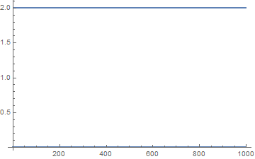
Let’s start with $m=6$ , this integer as discussed above satisfies periodicity with prime prime $L=2$ such that $\sigma_{k}(m)\bmod m=2$ for even $k$ integer and $\sigma_{k}(m)\bmod m=0$ ,for odd $k$ .see discret plot Figure 3.

$$\{0,2,0,2,0,2,0,2,0,2,0,2,0,2,0,2,0,2,0,2,0,2,0,2,0,2,0,2,0,2,0,2$$

$$,0,2,0,2,0,2,0,2,0,2,0,2,0,2,0,$$

$$2,0,2,0,2,0,2,0,2,0,2,0,2$$

$$,0,2,0,2,0,2,0,2,0,2,0,2,0,2,0,2,0,2,0,$$

$$2,0,2,0,2,0,2,0,2,0,2,0,2,0,2,0,2,0,2,$$

$$0,2,0,2,0,2,0,2,0,2,0,2,0,2,0,2$$

$$\}$$

Figure 3: Discrete plot for $\sigma_{k}(6)\bmod 6$,$k=0,10^{3}$

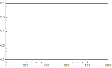
Now for $m=12$, Also this integer satisfies periodicity with prime $L=2$ such that $\sigma_{k}(m)\bmod m=6$ for even $k$ integer and $\sigma_{k}(m)\bmod m=4$ ,for odd $k$ .see discrete plot Figure 4.

$$\{4,6,4,6,4,6,4,6,4,6,4,6,4,6,4,6,4$$

$$,6,4,6,4,6,4,6,4,6,4,6,4,6,4,6,4,6,$$

$$4,6,4,6,4,6,4,6,4,6,4,6,4,6,4,6,4,6,4,6,4,6,4,6,$$

$$4,6,4,6,4,6,4,6,4,6,4,6,4,6,4,6,4,6,4,6,4,6,4,6,4,6,4,6,4,6,4,6,4,$$

$$6,4,6,4,6,4,6,4,6\}$$

Figure 4: Discrete plot for $\sigma_{k}(12)\bmod 12$,$k=0,10^{3}$

for $m=24$, Also this integer satisfies periodicity with prime $L=2$ such that $\sigma_{k}(24)\bmod 24=12$ for even $k$ integer and $\sigma_{k}(m)\bmod m=10$ ,for odd $k$ .see discrete plot Figure 5.

Figure 5: Discrete plot for $\sigma_{k}(12)\bmod 12$,$k=0,10^{3}$

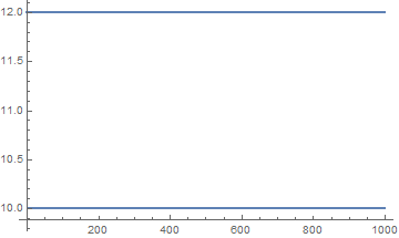
We may discuss in the following section statistics and the fitting distribution which is describe the behavior of the sequence $\sigma_{k}(m)\bmod m=0$ for some values of integers $m$,the interesting values in this paper are values whose satisfies periodicity with small period say:$m=6,12,24$.

4 Statistics and fit distribution of $\sigma_{k}(m)\bmod m$

Probability distribution fitting or simply distribution fitting is the fitting of a probability distribution to a series of data concerning the repeated measurement of a variable phenomenon.[14] The aim of distribution fitting is to predict the probability or to forecast the frequency of occurrence of the magnitude of the phenomenon in a certain interval.Distribution fitting is the procedure of selecting a statistical distribution that best fits to a data set generated by some random process.In other words, if we have some random data available, and would like to know what particular distribution can be used to describe our data, then distribution fitting is what we are looking for .

We consider the problem of selecting a probability distribution to represent a set of data , namely ,the data generated from the sequence $\sigma_{k}(m)\bmod m$,It has been pointed out that there are several criteria that can be considered when making this choice [16].

The aim is to use all of these criteria when making the choice, rather than select one criterion for this purpose. To illustrate, Wang et al provided data from an engineering problem involving machine tool [15]. They present five criteria:

• deviation in skewness and kurtosis,

• average deviation between the theoretical probability distribution function and the empirical one,

• average deviation between the theoretical cumulative distribution function and the empirical one,

• the Kolmogorov-Smirnov test statistic

• a subjective score (obtained from a group of experts in the field of study and statistics) on the user friendliness of the distribution and the frequency of its use in the field, and the fitness of properties and characteristics of the distribution to the sampled data

Our purpose in the present paper is attempt for making the final choice of distribution of the sequence $\sigma_{k}(m)\bmod m$ for some integers $m$ . let’s start with $m=6$,the given data for this case is already given in the precedent section ,recall :

data=

$$\begin{split}\{0,2,0,2,0,2,0,2,0,2,0,2,0,2,0,2,0,2,0,2,0,2,0,2,0,2,0,2,0,2,0,2&\\ ,0,2,0,2,0,2,0,2,0,2,0,2,0,2,0,&\\ 2,0,2,0,2,0,2,0,2,0,2,0,2&\\ ,0,2,0,2,0,2,0,2,0,2,0,2,0,2,0,2,0,2,0,&\\ 2,0,2,0,2,0,2,0,2,0,2,0,2,0,2,0,2,0,2,&\\ 0,2,0,2,0,2,0,2,0,2,0,2,0,2,0,2\\ \}\end{split}$$ (9)

We may start by giving the smooth histogram data which is defined in (9). Using mathematica Code we obtained the following smooth histogram for the given data $(casem=6)$ such that it seems looks follow the normal distribution , see Figure6:

Figure 6: Smooth Histogram for $\sigma_{k}(6)\bmod 6$ ,$k,0,10^{2}$

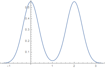
An important aspect of the description of a variable is the shape of its distribution, which tells you the frequency of values from different ranges of the variable.

Typically, a researcher is interested in how well the distribution can be approximated by the normal distribution [17]. Simple descriptive statistics can provide some information relevant to this issue. For example, if the skewness (which measures the deviation of the distribution from symmetry) is clearly different from 0, then that distribution is asymmetrical, while normal distributions are perfectly symmetrical. If the kurtosis (which measures peakedness of the distribution) is clearly different from $0$, then the distribution is either flatter or more peaked than normal; the kurtosis of the normal distribution is $0$.

More precise information can be obtained by performing one of the tests of normality to determine the probability that the sample came from a normally distributed population of observations. For example, the so-called Kolmogorov-Smirnov test [18], or the Shapiro-Wilk W test. However, none of these tests can entirely substitute for a visual examination of the data using a histogram (i.e., a graph that shows the frequency distribution of a variable). To easily generate a histogram from a spreadsheet, right-click on a cell within the desired variable and select Histogram from the Graphs of Input Data shortcut menu .For significance tests including tests of fit there is a hypothesized condition (called null hypothesis or $H_{0}$) that one is testing to see if it is true. For a test of fit the hypothesized condition is that the selected distribution generated the data. For a test that the means are equal, the hypothesized condition is equal means. The p-value is then probability that the data or one more extreme than it would have been generated under the hypothesized condition. A p-value of $0.05$ would indicate that the chance of the observed data is low, $1$ in $20$, due to variation alone. This is good evidence that the data was not generated under the hypothesized condition. The hypothesized condition is rejected if the p-value is $0.05$ or below. This provides $95\%$confidence the hypothesized condition is not true, i.e., the data does not fit the selected distribution or the means are not the equal.

The smaller the $p-value$, the greater the evidence that the data did not come from the selected distribution. For tests of fit and other tests, the confidence level is calculated from the p-value as 100*(1 - p-value).

The Shapiro-Wilks test for normality [27] is one of three general normality tests designed to detect all departures from normality. It is comparable in power to the other two tests.

The test rejects the hypothesis of normality when the p-value is less than or equal to $0.05$. Failing the normality test allows us to state with $95\%$ confidence the data does not fit the normal distribution. Passing the normality test only allows us to state no significant departure from normality was found.

The fit distribution of the sequence $\sigma_{k}(6)\bmod 6$ is presented in the following table. for $k=1$ to $10^{3}$

$$\left(\begin{array}[]{ccc}\text{}&\text{Statistic}&\text{P-Value}\\ \text{Anderson-Darling}&17.9641&\text{8.001946345268845$\grave{}$*${}^{\wedge}$-10}\\ \text{Baringhaus-Henze}&-\frac{200\exp\left(-\frac{99\ 3^{2/5}}{80\sqrt[5]{5}\left(1+\frac{1}{2}3^{2/5}5^{4/5}\right)}\right)}{\sqrt{1+\frac{1}{2}3^{2/5}5^{4/5}}}+\frac{1}{50}\left(2450+2500e^{-\frac{99\ 3^{2/5}}{20\sqrt[5]{5}}}\right)+\frac{100}{\sqrt{1+3^{2/5}5^{4/5}}}+1&\text{3.894223832290322$\grave{}$*${}^{\wedge}$-10}\\ \text{Cram{\'{e}}r-von Mises}&2.91772&0.\\ \text{Jarque-Bera ALM}&18.2108&0.00668519\\ \text{Mardia Combined}&18.2108&0.00668519\\ \text{Mardia Kurtosis}&-5\sqrt{\frac{2}{3}}&0.0000445571\\ \text{Mardia Skewness}&0&1.\\ \text{Pearson }\chi^{2}&550.&\text{8.96348580211817$\grave{}$*${}^{\wedge}$-112}\\ \text{Shapiro-Wilk}&0.636401&\text{2.233601575749124$\grave{}$*${}^{\wedge}$-14}\\ \end{array}\right)$$

Analysis of the obtained tests in the above table show that all tests regarding distribution of the sequence $\sigma_{k}(6)\bmod 6$ except skewness seem to have very small $p$ values close to $0$, suggesting they think this or more extreme data (in a sense appropriate to that test) is unlikely to be seen in a sample from a normal distribution , We used mathematica code to find five best distributions for the given data we got Empirical distribution [26] and discrete uniform distribution.

More than that one can use Kolmogorov Smirnov test which gives $0.561124$ using mathematica thus the probability that the sample (the given data) came from a Empirical distributed population of observations. see Figure 7

Figure 7: Kolmogorov Smirnov test for $\sigma_{k}(6)\bmod 6$ ,$k,0,10^{2}$, Kst=0.561124

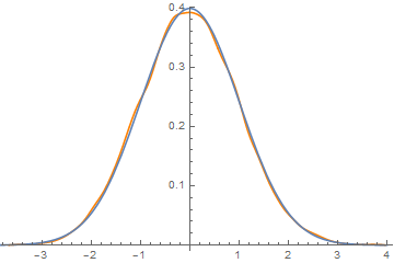
we obtained similar test analysis with $m=12,24$ by means the obtained tests indicate that the given data also follow the normal distribution.We have calculated the correspending PDF(probability density function) for $m=6,12,24$ are defined by order as :

$$f_{6}(x)=\frac{e^{-\frac{1}{2}(x-1)^{2}}}{\sqrt{2\pi}}$$

the mean is $1$ and variance $1$

$$f_{12}(x)=0.398942e^{-0.5(x-5.)^{2}}$$

the mean is $5$ and variance $1$

$$f_{24}(x)=0.398942e^{-0.5(x-11.)^{2}}$$

the mean is $11$ and variance $1$ When $m$ is selected to be a prime number ,every prime number satisfied periodicity with period $0$, it is easy to show that , one can calculate $\sigma_{k}(p)\bmod p$ thus gives $p^{k}+1\bmod p=1$ for every positive integer $k$.

Now, one can investigate about linear model which describes the relationship between a continuous response variable and one or more explanatory variables using a linear function.We were able to determine the linear model for the distribution of the sequence $\sigma_{k}(m)\bmod m$ for interesting numbers which satisfies periodicity with small period in $k$, The fit linear model for $m=6,12,24$ are the following affine function by order:

$$y=0.000150004x+0.984925$$

$$y=0.000150004x+4.98492$$

$$y=11.0151\,-0.000150004x$$

In the case $m=p$ the linear fit model given by this affine equation: $y=1$

we noted that the coefficient $a$ of the linear fit model for known integers with small periodictiy very close to $0$ with the same value of $b=0.000150004$ and identically $0$ with $b=1$ for the case $m$ is a prime number .For the correlation matrix (one can see the definition of this matrix in ([19]) is obtained and it is the same for all integers which are satisfying periodicity with small period such that it is given by the following form:

$$\left(\begin{array}[]{cc}1.&-0.867105\\ -0.867105&1.\\ \end{array}\right)$$

The Eigenvalues of this matrix are :$\{1.8671,0.132895\}$ it is symetric and definite positive matrix ,Where the eigenvectors of this matrix is :

$$\left(\begin{array}[]{cc}-0.707107&0.707107\\ -0.707107&-0.707107\\ \end{array}\right)$$

As our first eigenvector is $(\sqrt{2},\sqrt{2})$, the other eigenvector is uniquely (we’re in 2D) up to factor $1$/$-1$ the vector $(\sqrt{2}-\sqrt{2})$. So you get your diagonalizing orthogonal matrix as

$$\sqrt{2}\left[\begin{array}[]{cc}1&1\\ 1&-1\end{array}\right]$$

No we can reconstruct the covariance matrix to have the shape

$$\left[\begin{array}[]{cc}a+b&a-b\\ a-b&a+b\end{array}\right]$$

$a$ and $b$ are the eigenvalues. We would suggest to look closely on our model or the origin of the data. Then we might find a reason why our data may be distributed as $X_{1}=X_{a}+X_{b}$ and $X_{2}=X_{a}-X_{b}$, where $Var(X_{a})=a$ and $Var(X_{b})=b$ and $X_{a}$ and $X_{b}$ are independent.

If our data would follow a continuous multivariate distribution, it is almost sure that our correlation matrix follows from this sum/difference relation. If the data follow a discrete distribution, it is still very likely that the model $X_{1}=X_{a}+X_{b}$ and $X_{2}=X_{a}-X_{b}$ describes our data properly.

The distribution chart of this matrix is ploted in the following Figure ,see Figure 8:

Figure 8: Distribution chart of the given correlation matrix of our model

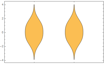
CookDistances Here is the plot of our model " CookDistances " up to 200 data .see Figure 9

Figure 9: Model plot "Cook distance" of the given data

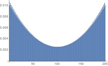
We may generate the random matrix [21] for this model ,namely , for the data genertaed by the sequence $\sigma_{k}(m)\bmod m$ such that $m$ always satisfies periodicity with small periode , we were able to generate the random matrix for the model correspending to the behavior of the sequence $\sigma_{k}(m)\bmod m$ , with the random choice $2$ and with symetric with the random domain ,Dom=$\{-2,2\}$ ,the correspending random matrix of dimension $(4\times 4)$is given as follow ( for $m=6$ ):

$$\left(\begin{array}[]{cccc}0.672103&0.00470158&-0.841173&-0.550396\\ 4.29385&0.387436&-0.531577&-1.47103\\ 0.110922&1.06249&-0.0840228&2.14514\\ 0.324367&0.113398&-0.969011&0.105082\\ \end{array}\right)$$

The eigenvalues of the obtained random matrix are :$\{0.555432\,+1.82595i,0.555432\,-1.82595i,-0.53802+0.i,0.507754\,+0.i\}$, According to our computations on many examples using mathematic it seems that the behavior of eigenvalues of random matrix very related to the Random domain this mean that if we would have small length Random domain we would have real eigenvalues between $(0,1)$ as we noted in the precedent random matrix., we may discuss this point in the last section which related to the equivalence of the Riemann hypothesis . as a conclusion of this section and based on the achieved numerical evidence that we have done the behavior of the iterative sequence $\sigma_{k}(m)\bmod m$ follows the normal distribution for integers satisfying periodicity with small period and also even for large period.

5 discussion and analysis of result 3

We all know what prime numbers are. Euclid has proven that there are infinitely many of them. Experience has taught us that they get more rare when we come to ever higher numbers. Of course mathematicians want to describe the "statistics" of the primes in more precise terms. The prime number theorem (proven at the end of the $19^{\rm th}$ century) tells us that there are about $n/\log n$ primes $\leq n$ when $n$ is large. The next question then is: How much can the true number $\pi(n)$ deviate from this estimate? Working on this problem already Riemann has remarked that there is a huge technical stumbling block, nowadays called the "Riemann Hypothesis"[28]. So far nobody has managed to move this block away. Therefore mathematicians go around it: Many papers have a proviso in their introduction: "Assuming that the Riemann Hypothesis is true, we prove the following: $\>\ldots\>$,One may interpret the Riemann Hypothesis by saying that the primes are distributed as egularly as possible: for any real number $x$ the number of prime numbers less than $x$ is approximately $Li(x)$ and this approximation is essentially square root accurate. More precisely,

$$\pi(x)=Li(x)+O(\sqrt{x}\log(x)).$$

The Riemann Hypothesis says that all non-trivial zeros of the Riemann zeta function lie on $Re(z)=\frac{1}{2}$ line instead this region $Re(z)\in(0,1)$.

We claimed above that the Riemann hypothesis is false if and only if there exist a pair of positive integers $(m,k)$ such that $\sigma_{k}(m)\bmod m$ is not periodic in $k$ , we may consider this result as unconditional equivalence such that no strong proof exists for instance but we may explain this result based on our numerical evidence and using some obtained results in random matrix theory .Firstly we may need to give a brief survey about random matrices ,In probability theory and mathematical physics, a random matrix is a matrix-valued random variable—that is, a matrix in which some or all elements are random variables. Many important properties of physical systems can be represented mathematically as matrix problems. For example, the thermal conductivity of a lattice can be computed from the dynamical matrix of the particle-particle interactions within the lattice.Random matrices have been a very active area of research for the last few decades and have found enormous applications in various areas of modern mathematics, physics, engineering, biological modeling, and other fields.[24]

A random symmetric $2\times 2$ matrix $A=\begin{pmatrix}a_{11}&a_{12}\\ a_{12}&a_{22}\end{pmatrix}$ is a member of the gaussian orthogonal ensemble (GOE), if it satisfies three conditions:

• 1) for any $2\times 2$ orthogonal transformation $OO^{T}=I=O^{T}O$, $A^{\prime}=OAO^{T}$ is also a member of the GOE.

• 2) the matrix elements $a_{11},a_{12}$ and $a_{22}$ are statistically independent.

• 3) the probability density $P(A)dA$, where $dA=da_{11}da_{12}da_{22}$ is given by

  $$P(A)\propto e^{-aTrA^{2}+bTrA+c}$$

  where $a>0,b$ and $c$ are real numbers.

Let $x=\sigma_{k}(m)\bmod m$ be a random integer more than that we may consider $x$ as a complex random variable by the assumption of $m$being Gaussian integers iid(independent identicaly distributed),with non zero finit variance , we are already showed in the precedent section that $x$ follow Empirical distribution and its variable are independent using numerical evidence(fit test model) ,now assume the generated data by $x$ would follow a continuous multivariate distribution thus we have continuous uniforme distribution thus their spectra converge to the semicircular law when $m$ grows, the case of $n=2^{m}-1$ which called Golomb sequences is already shown in [25], Assume the sequence $\sigma_{k}(m)\bmod m$ is not periodic in $k$ for some integers $(m,k)$ this means for some integer $(m,k)$ the sequence $\sigma_{k}(m)\bmod m$ is unbounded one can show this easly using the extreme value theorem for continuous functions which states that every continuous function defined on a closed and bounded interval attains its maximum and minimum value. Thus, $f(x)$ is bounded on the closed bounded interval $[0,p]$

Therefore there exists a positive rel number B such that

$$|f(x)|\leq B$$

for

$$x\in[0,p]$$

The periodicity implies that it is bounded on real line because

$$|f(kp+x)|=|f(x)|\leq B$$

for all integers $k.$

Note that every real number could be represented as $x+kp$ where $k$ is an integer and $x\in[0,p].$ Now by the assumption of the sequence $\sigma_{k}(m)\bmod m$ being unbounded this $x$ is unbounded this contradict the famous Circular law conjecture which it is proved by Terence Tao and VAN VU in [22] using strong version which states that :The strong circular law holds for any complex variable $x$ with zero mean and finite non-zero variance. and they considered the spectral density for empirical distribution ,In [23] , Bai proved the claim under the assumption that $x$ has finite sixth moment $(E|x|^{6}<\infty)$ and that the joint distribution of the real and imaginary parts of $x$ has a bounded density.The sequence $\sigma_{k}(m)\bmod m$ is unbounded lead the random complex variable $x$ to be unbounded which gives immediately both of imaginary part and its real part with unbounded density .The well known relationship between circular law and Riemann zeta zeros is that it has been conjectured that the limiting distribution of the non-trivial zeros of the Riemann zeta function (and other L-functions), on the scale of their mean spacing, is the same as that of the eigenphases $\theta_{n}$ of matrices in the CUE(circular unitary ensemble) in the limit as $n\to\infty$ [32],[33] ,[34]

A weaker reason to show that result hold ,namely , the equivalence of the Riemann hypothesis is to find such relationship between periodicity of the sequence $x=\sigma_{k}(m)\bmod m$ and the orthogonality and symmetry (entries of Random variable iid) of the expected random matrice for the Riemann hypothesis to be hold ,one can refer to [25] .

6 Futur work (New model to proof RH)

We may use our new fit model which uses periodicity of the sequence $\sigma_{k}(m)\bmod m$to expect and predict the random matrix to proof the Riemann hypothesis such that we may attempt to investigate about the behavior of its eigenvalues comparing it with behavior of nontrivial zero of Riemann zeta functon and for only one purpose which is to get such random matrix where its eigenvalues are real [29] , we may suggest $x$ as a complex random variable such that follow the empirical distribution with bounded density such that we may consider : $x_{i+1}=\sigma_{k}(m+1)\bmod(m+1),x_{i}=\sigma_{k}(m)\bmod(m)$, let $m$ be Gaussian integers , we define a new complex random variable $y$ distributed as : $Y_{i}=x_{i+1}-x_{i}$ , $i$ is positive integer $j,i=0,n$ and $Y_{j}=x_{j+1}+x_{j}$looking to its periodicity in $k$ , The complex random variable $Y_{i}=x_{i+1}-x_{i}$ will tel us much about distribution of prime numbers ,in particularly gaps between primes [30] which it is recently the aim of researchers .

6.1 Appendix for result 1

A more challenging problem is to ask for integers $m$ and $p$ such that for all integers $k$, $p_{0}=p,p_{k+1}=\sigma(p_{k}),$ and $p_{k}=0\bmod m$. The current problem adds the restriction that $p=m$, which implies $m$ is a multiperfect number. Since multiperfect numbers are rare, it should be hard to find a metaperfect number, a number $m$ that satisfies $\sigma^{k}(m)=0\bmod m$ for all iterations of $\sigma$.

Indeed, $\sigma(m)<m\omega(m)$ for most values of $m$, so for a potentially metaperfect number to exist, we can’t depend on $\sigma(p_{k})/m$ to be coprime to $m$ for very many $k$. More likely, $\sigma(p_{k})/m$, if integral, will share a small factor with $m$ and further iterations of $\sigma$ will avoid certain large prime factors of $m$. This is what was observed, and what I hoped to prove and did not in the other answer.

It is an interesting side question to determine $\min_{k}g_{k}$ where $g_{0}=p_{0}$ and $g_{k+1}=\gcd(p_{k+1},g_{k})$. In particular, do the iterates of $\sigma$ encounter a square or twice a square, regardless of the starting point? If so, then the minimum is odd and likely 1. Otherwise $p$ is a seed for $m$, and $p$ might be useful in looking for multiperfect numbers which are multiples of $m$.

Cohen and te Riele investigated a weaker question: Given $n$ is there a $k$ for which $\sigma^{k}(n)=0\bmod n$? They did this in a 1996 paper and asserted through computation that the answer was yes for $n\leq 400$. Their data suggest to us both that the weaker question has an affirmative answer, and that there are no metaperfect numbers or even seeds for a number.

Aknowledjements I would like to thank Gerarld .R. Paseman From MO for his great contributions to this paper(Indication for proofs, Appendix) and for his encouragements to produce the best of the best for number theory field .

References

- [1] Euclid The Thirteen Books of Euclid’s Elements, translated by T.L. Heath, Cambridge University Press, vol. 2, 1908.
- [2] L. Euler De numeris amicabilibus, in Opera Postuma mathematica et physica, 1862 p. 88, Saint Petersburg Academy of Science
- [3] P. Ochem and M. Rao Odd perfect numbers are greater than 101500, Comp. 81 (2012), 1869–1877
- [4] Graeme L. Cohen and Herman J. J. te Riele . Iterating the Sum of Divisors Function. 1991 Mathematics Subject Classification: 11A25, 11Y70, the c A K Peters, Ltd. 1058,6458/96
- [5] P. Erdos, A. Granville, C. Pomerance, and C. Spiro. On the normal behavior of the iterates of some arithmetical functions.204 in Analytic Number Theory, Allerton Park, 1989
- [6] R. K. Guy Unsolved Problems in Number Theory. Springer, New York, , 1994.
- [7] P.Erdos ,A.Granville ,C.pomerance and S.Spiro on the normal behavior of the iterates of some arithmitic function printed in the united states of americain . Edited by :Brace C Berndt, Harold G Diamond , Heini Helberstam, Adolf Hildebrand , 1990.
- [8] Maier On the third iterates of the phi, and sigma functions. Institute of Mathematics Polish Academy of Sciences,Colloquium Mathematicum , 1984 ,1985 | 49 | 1 | 123,130
- [9] Paul Pollack and Carl Pomerance Some problems of Erdős on the sum of divisors function. AMS Journal: Trans. Amer. Math. Soc. Ser. B 3 (2016), 1, 26,DOI: https://doi.org/10.1090/btran/10 , April 5, 2016
- [10] P.Erdos On the asymptotic properties of aliquot sequences. A MATHEMATICS OF COMPUTATION, VOLUME 30, NUMBER 135 JULY 1976, PAGES 641,645, 1976
- [11] Lenstra Problem 6064, Amer. Math. Monthly 82 (1975). , 1016. Solution by the proposer, op. cite. 84 (1977), 580, 1977
- [12] YoungJu CHOIE, Nicolas LICHIARDOPOL, Pieter MOREE et Patrick SOLE On Robin’s criterion for the Riemann hypothesis , Journal de Th´eorie des Nombres de Bordeaux 19 (2007), 357–372
- [13] Robin, Guy Frequency and Regression Analysis Journal de Mathématiques Pures et Appliquées, Neuvième Série, 63 (2): 187–213,1984
- [14] H.P.Ritzema Drainage Principles and Applications, Publ. 16, pp. 175–224 International Institute for Land Reclamation and Improvement (ILRI), Wageningen, The Netherlands. ISBN 9070754339.
- [15] Wang, Y., Yam, R.C.M., and Zuo, M.J. A multi-criterion evaluation approach to selection of the best statistical distribution Computers and Industrial Engineering, 47, 165-180.
- [16] Pomerol, J-C, and Barba-Romero Multicriterion Decision in Management – Principles and Practice Kluwer, Boston.2000
- [17] Richard G. Brereton The normal distribution Wiley Analytical Science journal 2014 ,https://doi.org/10.1002/cem.2655
- [18] Galen R. Shorack et Jon A. Wellner Empirical Processes With Applications to Statistics Philadelphie, Society for Industrial Applied Mathematics, 4 septembre 2009, 998 p. (ISBN 978-0-89871-684-9 et 0-89871-684-5, LCCN 2009025143
- [19] J.Ferré 3.02 - Regression Diagnostics Comprehensive Chemometrics Chemical and Biochemical Data Analysis 2009, Pages 33-89
- [20] Alan Edelman Random matrix theory Acta numerica 2005,pp 1. 165,campridge university press ,printed in the united kingdom
- [21] Alan Edelman Random matrix theory Acta numerica 2005,pp 1. 165,campridge university press ,printed in the united kingdom
- [22] TERENCE TAO AND VAN Vu RANDOM MATRICES: THE CIRCULAR LAW https://arxiv.org/pdf/0708.2895.pdf
- [23] Z. D. Bai Circular law Ann. Probab. 25 (1997), 494–529
- [24] G. Akemann, J. Baik, and P. Di Francesco The Oxford handbook of random matrix theory, Oxford University Press, 2011.
- [25] Ilya Soloveychik, Yu Xiang and Vahid Tarokh Symmetric Pseudo-Random Matrices John A. Paulson School of Engineering and Applied Sciences, Harvard University Dedicated to the memory of Solomon W. Golomb (1932-2016)
- [26] Peter Gaenssler, Pál Révész Empirical Distributions and Processes selected Papers from a Meeting at Oberwolfach, March 28 - April 3, 1976,springer
- [27] Elizabeth González-Estrada, José A. Villasenor and Rocio Acosta-Pech Shapiro-Wilk test for multivariate skew-normality Computational Statistics volume 37, pages1985–2001 (2022),springer
- [28] J. P. Keating, N. C. Snaith Random Matrix Theory and BRIMS, Hewlett-Packard Laboratories, Filton Road, Stoke Gifford, Bristol BS34 6QZ, UK Received: 20 December 1999 / Accepted: 24 March 2000
- [29] john Peca-Medlin An Approach to the Riemann Hypothesis through Random Matrix Theory Department of Mathematics University of California, Irvine June 10, 2018
- [30] James Maynard Large gaps between primes https://arxiv.org/abs/1408.5110
- [31] Zeraoulia Rafik On congruence of the iterated form https://arxiv.org/abs/2102.09941
- [32] Montgomery, H.L The pair correlation of the zeta function. Proc. Symp. Pure Math. 24, 181–93 (1973)
- [33] Odlyzko, A.M The 10 power 20 th zero of the Riemann zeta function and 70 million of its neighbors. Preprint, 1989
- [34] Rudnick,Z. and Sarnak, P Zeros of principal L-functions and random-matrix theory Duke Math. J. 81, 269–322 (1996)