Best-Response Dynamics in Two-Person Random Games with Correlated Payoffs

Abstract

We consider finite two-player normal form games with random payoffs. Player $\mathrm{A}$’s payoffs are i.i.d. from a uniform distribution. Given $p\in[0,1]$, for any action profile, player $\mathrm{B}$’s payoff coincides with player $\mathrm{A}$’s payoff with probability $p$ and is i.i.d. from the same uniform distribution with probability $1-p$. This model interpolates the model of i.i.d. random payoff used in most of the literature and the model of random potential games. First we study the number of pure Nash equilibria in the above class of games. Then we show that, for any positive $p$, asymptotically in the number of available actions, best response dynamics reaches a pure Nash equilibrium with high probability.

[labelLuiss]organization=Dipartimento di Economia e Finanza, Luiss University, addressline=Viale Romania 32, city=Roma, postcode=00197, state=RM, country=Italy

[labelSapienza]organization=Dipartimento di Matematica “Guido Castelnuovo”, Sapienza Università di Roma, addressline=Piazzale Aldo Moro 5, city=Roma, postcode=00185, state=RM, country=Italy

1 Introduction

1.1 The problem

Consider the class of two-person normal-form finite games. Some properties hold for the entire class, for instance, the mixed extension of each game in the class admits a Nash equilibrium (Nash,, 1950, 1951). Some properties hold generically, for instance, generically the number of Nash equilibria is finite and odd (Wilson,, 1971; Harsanyi,, 1973). Some properties do not hold generically and neither does their negation; for instance having a pure Nash equilibrium or not having a pure Nash equilibrium is a not a generic property of finite games. Still, it may be relevant to know how likely it is for a finite game to admit a pure equilibrium. Along a similar line of investigation, how likely is a recursive procedure—such as best response dynamics—to reach a pure Nash equilibrium in finite time?

One way to formalize these questions is to assume that the game is drawn at random according to some probability measure. It is not clear what a natural probability measure is in this setting; a good part of the literature on the topic has focused on measures that make the payoffs i.i.d. with zero probability of ties. Few papers have relaxed this assumption. For instance, Rinott and Scarsini, (2000) considered payoff vectors that are i.i.d. across different action profiles, but can have some positive or negative dependence within the same action profile. Amiet et al., 2021b considered i.i.d. payoffs whose distribution may have atoms and, as a consequence, may produce ties. Durand and Gaujal, (2016) studied the class of random potential games, i.e., a class of games that admit a potential having i.i.d. entries.

1.2 Our contribution

In this paper we want to study two-person games with random payoffs where the stochastic model for the payoffs parametrically interpolates the case of i.i.d. payoffs with no ties and the case of random potential games. In particular, we start with a model where all payoffs are i.i.d. according to a continuous distribution function (without loss of generality, uniform on $[0,1]$) and we consider an i.i.d. set of coin tosses, one for each action profile. If the toss gives head, then the original payoff of the second player is made equal to the payoff of the first player; if the toss gives tail, the payoff remains unchanged. The relevant parameter is the probability $p$ of getting heads in the coin toss. If $p=0$, we obtain the classical model of random games with continuous i.i.d. payoffs. If $p=1$, we get the model of common-interest random games. From the viewpoint of pure Nash equilibria any potential game is strategically equivalent to a common-interest game. Therefore, the above class of games parametrically interpolates the case of i.i.d. payoffs with no ties and the case of random potential games. When $p$ is small, the game is close to a game with i.i.d. payoffs; when $p$ is large, the game is close to a potential game.

For this parametric class of games we first compute the expected number of PNE as a function of $p$, and then study its asymptotic behavior as the numbers of actions of the two players diverge, possibly at different speeds. It is well known (Powers,, 1990) that, as the number of action increases, the asymptotic distribution of the number of PNE is a $\operatorname{\mathsf{Poisson}}(1)$ distribution, for i.i.d. random payoffs. Our result shows an interesting phase transition around $p=0$, in the sense that for every $p>0$ the expected number of PNE diverges.

We then consider best response dynamics (BRD) for the above class of games. Durand and Gaujal, (2016) considered BRD for random potential games with an arbitrary number of players and the same number of actions for each player. In this class of games a PNE is reached by a BRD in finite time. Durand and Gaujal, (2016) studied the asymptotic behavior of the expectation of this random time. In our paper we first consider potential games and we compute the distribution of the time that the BRD needs to reach a PNE. Moreover we compute exactly the first two moments of this random time, when the two players have the same action set.

Amiet et al., 2021a showed that, for games with i.i.d. continuous payoffs, when players have the same action set, as the number of actions increases, the probability that a BRD reaches a PNE goes to zero. Here we generalize the result of Amiet et al., 2021a to the case of possibly different action sets for the two players. Moreover, we prove that for every positive $p$, asymptotically in the number of actions, a BRD reaches a PNE in finite time with probability arbitrarily close to $1$. Again this shows a phase transition in $p=0$ for the behavior of the BRD.

1.3 Related literature

Games with random payoffs have been studied for more than sixty years. We refer the reader to Amiet et al., 2021b ; Heinrich et al., (2023) for an extensive survey of the literature on the topic. Here we mention just some recent papers and some articles that are more directly connected with the results of our paper. Powers, (1990) proved that in random games with i.i.d. payoffs having a continuous distribution, as the number of actions of at least two players diverges, the asymptotic distribution of the number of PNE is $\operatorname{\mathsf{Poisson}}(1)$. Stanford, (1995) computed the exact nonasymptotic form of this distribution, from which the result in Powers, (1990) can be obtained as a corollary. Rinott and Scarsini, (2000) retained the i.i.d. assumptions for payoff vectors corresponding to different action profiles, but allowed dependence for payoffs within the same profile. They proved an interesting phase transition in terms of the payoffs’ correlation: asymptotically in either the number of players or the number of actions, for negative dependence the number of PNE goes to $0$, for positive dependence it diverges, and for independence it is $\operatorname{\mathsf{Poisson}}(1)$, as proved by Powers, (1990). Baldi et al., (1989) studied the distribution of the number of local maxima on a graph, which—by choosing a suitable graph—can be translated into the number of PNE in a random potential game.

Pei and Takahashi, (2019) studied point-rationalizable strategies in two-person random games. Since the number of point-rationalizable strategies for each player is weakly larger than the number of PNE, they were interested in the typical magnitude of the difference between these two numbers. A game is dominance solvable if iterated elimination of strictly dominated strategies leads to a unique action profile, which must be a PNE. Alon et al., (2021) used recent combinatoric results to prove that the probability that a two-person random game is dominance solvable vanishes with the number of actions.

Several papers studied the behavior of various learning dynamics BRD in games with random payoffs. For instance, Galla and Farmer, (2013) studied a type of reinforcement learning called experience-weighted attraction in two-person games and showed the existence of three different regimes in terms of convergence to equilibria. Sanders et al., (2018) extended their analysis to games with an arbitrary finite number of players. Pangallo et al., (2019) compared through simulation the behavior of various adaptive learning procedures in games whose payoffs are drawn at random. Heinrich et al., (2023) compared the behavior of BRD in games with random payoffs, when the order of acting players is fixed vs when it is random and they showed that, asymptotically in either the number of players or the number of strategies, the fixed-order BRD converges with vanishing probability, whereas the random-order does converge to a PNE whenever it exists. Similar results were obtained by Wiese and Heinrich, (2022).

Coucheney et al., (2014); Durand and Gaujal, (2016); Durand et al., (2019) focused on random potential games and measured the speed of convergence of BRD to a PNE. Amiet et al., 2021a dealt with two-person games where the players have the same action set and payoffs are i.i.d. with a continuous distribution. They compared the behavior of best response dynamics and better response dynamics. They proved that, asymptotically in the number of actions, the first reaches a PNE only with vanishing probability, whereas the second does reach it, whenever it exists. Amiet et al., 2021b studied a class of games with $n$ players and two actions for each player where the payoffs are i.i.d. but their distribution may have atoms. They proved that the relevant parameter for the analysis of this class of games is the probability of ties in the payoffs, called $\alpha$. They showed that, whenever this parameter is positive, the number of PNE diverges, as $n\to\infty$ and proved a central limit theorem for this random variable. Moreover, using percolation techniques, they studied the asymptotic behavior of BRD, as a function of $\alpha$, and they showed a phase transition at $\alpha=1/2$. Johnston et al., (2023) considered the class of games whose random payoffs are i.i.d. with a continuous distribution; they showed that in almost every game in this class that has a pure Nash equilibrium, asymptotically in the number of players, best response dynamics can lead from every action profile that is not a pure Nash equilibrium to every pure Nash equilibrium.

Potential functions in games were introduced by Rosenthal, (1973) and their properties were extensively studied by Monderer and Shapley, (1996). Among them, existence of PNE and convergence to one of these equilibria of the most common learning procedures, including BRD.

Goemans et al., (2005) introduced the concept of sink equilibrium. Sink equilibria are strongly connected stable sets of action profiles that are never abandoned once reached by a BRD. A sink equilibrium that is not a PNE is what in this paper is called a trap.

Fabrikant et al., (2013) studied the class of weakly acyclical games, i.e., the class of games for which from every action profile, there exists some better-response improvement path that leads from that action profile to a PNE. This class includes potential games and dominance solvable games as particular cases.

The goal of our paper is to consider probability measures on spaces of finite noncooperative games that go beyond the usual assumption of i.i.d. payoffs. In particular, we define a parametric family of probability measures that interpolates random games with i.i.d. payoffs and random potential games. The interpolation is achieved locally by acting on each action profile of the game and replacing—with some fixed probability and independently across profiles—the payoff of the second player with the payoff of the first player. A different interpolation could be achieved by considering a convex combination of a game with i.i.d. payoffs and a random potential game. This was done, e.g., in Rinott and Scarsini, (2000), where in each action profile the payoffs are obtained by summing a Gaussian vector with i.i.d. components and an independent Gaussian vector with identical components (which plays the role of the random potential). This approach is somehow comparable with the idea of decomposing the space of finite games proposed by Candogan et al., (2011). This decomposition was then used by Candogan et al., (2013) to analyze BRD in games that are close to potential games.

1.4 Organization of the paper

Section 2 introduces some basic game theoretic concepts. Section 3 defines the parametric family of distributions on the space of games and deals with the number of PNE in games with random payoffs. Section 4 studies the behavior of BRD in games with random payoffs in the above parametric class, for different values of the parameter. Section 5 contains all the proofs. Conclusions and open problems can be found in Section 6. Appendix A lists the symbols used throughout the paper. Appendix B contains two well-known results about the Beta distribution.

1.5 Notation

Given an integer $n$, the symbol $[n]$ indicates the set $\{1,\dots,n\}$. Given a finite set $A$, the symbol $\lvert A\rvert$ denotes its cardinality. The symbol $\sqcup$ denotes the union of disjoint sets. We use the notation $x\wedge y\coloneqq\min\{x,y\}$. The symbol $\xrightarrow{\mathsf{P}}$ denotes convergence in probability.

Given two nonnegative sequences $h_{n},g_{n}$, we use the following common asymptotic notations:

$$h_{n}=o(g_{n})\quad \text{if}\quad\lim_{n\to\infty}\frac{h_{n}}{g_{n}}=0,$$ (1.1)

$$h_{n}=\mathcal{O}(g_{n})\quad \text{if}\quad\limsup_{n\to\infty}\frac{h_{n}}{g_{n}}<\infty,$$ (1.2)

$$h_{n}=\Omega(g_{n})\quad \text{if}\quad\liminf_{n\to\infty}\frac{h_{n}}{g_{n}}>0,$$ (1.3)

$$h_{n}=\omega(g_{n})\quad \text{if}\quad\lim_{n\to\infty}\frac{h_{n}}{g_{n}}=\infty,$$ (1.4)

$$h_{n}=\Theta(g_{n})\quad \text{if}\quad h_{n}=\mathcal{O}(g_{n})\quad\text{and}\quad h_{n}=\Omega(g_{n}).$$ (1.5)

2 Preliminaries

We consider two-person normal-form games where, for $i\in\{\mathrm{A},\mathrm{B}\}$, player $i$’s action set is $[K^{i}]\coloneqq\left\{1,\dots,K^{i}\right\}$ and $U^{i}\colon[K^{\mathrm{A}}]\times[K^{\mathrm{B}}]\to\mathbb{R}$ is player $i$’s payoff function. The game is defined by the payoff bimatrix

$$\boldsymbol{U}\coloneqq(\boldsymbol{U}^{\mathrm{A}},\boldsymbol{U}^{\mathrm{B}}),$$ (2.1)

where, for $i\in\{\mathrm{A},\mathrm{B}\}$,

$$\boldsymbol{U}^{i}\coloneqq(U^{i}(a,b))_{a\in[K^{\mathrm{A}}],b\in[K^{\mathrm{B}}]}.$$ (2.2)

A pure Nash equilibrium (PNE) of the game is a pair $(a^{\ast},b^{\ast})$ of actions such that, for all $a\in[K^{\mathrm{A}}],b\in[K^{\mathrm{B}}]$ we have

$$U^{\mathrm{A}}(a^{\ast},b^{\ast})\geq U^{\mathrm{A}}(a,b^{\ast})\quad\text{and}\quad U^{\mathrm{B}}(a^{\ast},b^{\ast})\geq U^{\mathrm{B}}(a^{\ast},b).$$ (2.3)

As is well known, PNE are not guaranteed to exist. A class of games that admits PNE is the class of potential games, i.e., games for which there exists a potential function $\Psi\colon[K^{\mathrm{A}}]\times[K^{\mathrm{B}}]\to\mathbb{R}$ such that for all $a,a^{\prime}\in[K^{\mathrm{A}}]$, for all $b,b^{\prime}\in[K^{\mathrm{B}}]$, we have

$$U^{\mathrm{A}}(a,b)-U^{\mathrm{A}}(a^{\prime},b)=\Psi(a,b)-\Psi(a^{\prime},b),$$ (2.4a)

$$U^{\mathrm{B}}(a,b)-U^{\mathrm{B}}(a,b^{\prime})=\Psi(a,b)-\Psi(a,b^{\prime}).$$ (2.4b)

Games of common interest, i.e., games for which $U^{\mathrm{A}}=U^{\mathrm{B}}$, are a particular case of potential games. As far as PNE are concerned, every potential game is strategically equivalent to a common interest game, for instance to the game where $U^{\mathrm{A}}=U^{\mathrm{B}}=\Psi$. For the properties of potential games with an arbitrary number of players, we refer the reader to Monderer and Shapley, (1996).

Given a finite game, it is interesting to see whether an equilibrium can be reached iteratively by allowing players to deviate whenever they have an incentive to do so. In particular, we will consider a procedure where, starting from a fixed action profile, players in alternation choose their best response to the other player’s action. If the procedure gets stuck in an action profile, then it has reached a pure Nash equilibrium. In general, there is no guarantee that this occurs.

Assume that the payoffs of each player are all different, i.e., $U^{\mathrm{A}}(a,b)\neq U^{\mathrm{A}}(a^{\prime},b)$ for all $a\neq a^{\prime}$ and all $b$ (and similarly for the second player). The best response dynamics (BRD) is a learning algorithm taking as input a two-player game $(U^{\mathrm{A}},U^{\mathrm{B}})$ and a starting action profile $(a_{0},b_{0})$. For each $t\geq 0$ we consider the process $\operatorname{\mathsf{BRD}}(t)$ on $[K^{\mathrm{A}}]\times[K^{\mathrm{B}}]$ such that

$$\operatorname{\mathsf{BRD}}(0) =(a_{0},b_{0})$$ (2.5)

and, if $$\operatorname{\mathsf{BRD}}(t)=(a^{\prime},b^{\prime}) t$$, then, for even,

$$\operatorname{\mathsf{BRD}}(t+1) =(a^{\prime\prime},b^{\prime}),$$ (2.6)

where $$a^{\prime\prime}\in\operatorname*{arg\,max}_{a\in[K^{\mathrm{A}}]}U^{\mathrm{A}}(a,b^{\prime})\setminus\left\{a^{\prime}\right\}$$, if the latter set is not empty, otherwise

$$\operatorname{\mathsf{BRD}}(t+1) =\operatorname{\mathsf{BRD}}(t);$$ (2.7)

for $$t$$ odd,

$$\operatorname{\mathsf{BRD}}(t+1) =(a^{\prime},b^{\prime\prime}),$$ (2.8)

where $$b^{\prime\prime}\in\operatorname*{arg\,max}_{b\in[K^{\mathrm{B}}]}U^{\mathrm{B}}(a^{\prime},b)\setminus\left\{b^{\prime}\right\}$$, if the latter set is not empty, otherwise

$$\operatorname{\mathsf{BRD}}(t+1) =\operatorname{\mathsf{BRD}}(t).$$ (2.9)

It is easy to see that, if, for some positive $\hat{t}$, we have

$$\operatorname{\mathsf{BRD}}(\hat{t})=\operatorname{\mathsf{BRD}}(\hat{t}+1)=(a^{\ast},b^{\ast}),$$ (2.10)

then $\operatorname{\mathsf{BRD}}(t)=(a^{\ast},b^{\ast})$ for all $t\geq\hat{t}$ and $(a^{\ast},b^{\ast})$ is a PNE of the game.

The algorithm stops when it visits an action profile for the second time. If this profile is the same as the one visited at the previous time, then a PNE has been reached.

Inspired by the concept of sink equilibrium of Goemans et al., (2005), we give a definition of trap in a way that is suitable for our two-player environment.

Definition 2.1.

A trap is a finite set $M$ of action profiles such that

1. $\lvert M\rvert\geq 2$,

2. if $\operatorname{\mathsf{BRD}}(t)\in M$, then $\operatorname{\mathsf{BRD}}(t+1)\in M$;

3. for every $(a,b)\in M$, there exists $t$ such that $\operatorname{\mathsf{BRD}}(t+k\lvert M\rvert)=(a,b)$, for every $k\in\mathbb{N}$.

Moreover, the definition of BRD implies that for every trap $M$ we have $\lvert M\rvert\geq 4$ and $\lvert M\rvert$ even. Moreover, for every game $(U^{\mathrm{A}},U^{\mathrm{B}})$ and every initial profile $(a,b)$, the BRD eventually visits a PNE or a trap in finite time, say $\tau$.

Even if the game admits PNE, there is no guarantee that a BRD reaches one of them; it could cycle over a trap, i.e., it could start to periodically visit the same set of action profiles and never stabilize. On the other hand, if the game is a potential game, then a BRD always reaches a PNE. This is due to the fact that at every iteration of the BRD the payoff of one player increases, and so does the potential. Since the game is finite, in finite time the BRD reaches a local maximum, which is a PNE (see, e.g., Karlin and Peres,, 2017, proposition 4.4.6).

The goal of this paper is to study the number of PNE and the behavior of BRD in a “typical” game. To make sense of the above sentence, we need to formalize the meaning of the term typical. The approach that we will take is stochastic. That is, we will assume the bimatrix $\boldsymbol{U}$ to be random and drawn from a distribution that will be specified later. In any game with random payoffs, the set $\operatorname{\mathsf{NE}}$ of pure Nash equilibria is a (possibly empty) random set of action profiles, i.e., a random subset of $[K^{\mathrm{A}}]\times[K^{\mathrm{B}}]$. Therefore, since the game is finite, the number of PNE is an integer-valued random variable. Moreover, we will be able to speak about the probability that a BRD converges (to a PNE).

3 Number of pure Nash equilibria in random games

As mentioned in the Introduction, several attempts have been made in the literature to put a probability measure on a space of games. Most of the existing papers assume all the entries of $\boldsymbol{U}$ to be i.i.d. with a continuous marginal distribution. There are some notable exceptions to the independence assumption. Rinott and Scarsini, (2000) considered a setting where the payoff vectors of different action profiles have a continuous distribution and are i.i.d. ​​, but some dependence is allowed within each profile. Durand and Gaujal, (2016) studied random potential games where the entries of the potential are i.i.d. with a continuous distribution.

Our stochastic model is quite general, since—in a sense that will be made precise—it interpolates the i.i.d. payoffs and the random potential.

By definition, the concept of pure Nash equilibrium is ordinal, that is, if all payoffs in a game are transformed according to a strictly increasing function, then the set of pure Nash equilibria remains the same. Assume that each entry of $\boldsymbol{U}$ has a marginal distribution that is uniform on the interval $[0,1]$. Its distribution function will be denoted by $F$. The above consideration implies that this uniformity assumption is without loss of generality, i.e., any other continuous distribution would produce the same conclusions.

Start with $(\boldsymbol{U}^{\mathrm{A}},\boldsymbol{U}^{\mathrm{B}})$, where all the entries are i.i.d. with distribution $F$. Then, for each action profile $(a,b)$, with probability $p$ set $U^{\mathrm{B}}(a,b)$ to be equal to $U^{\mathrm{A}}(a,b)$, independently of the other action profiles. In other words, for every pair $(a,b)$,

• with probability $1-p$, the random payoffs $U^{\mathrm{A}}(a,b)$ and $U^{\mathrm{B}}(a,b)$ are independent,

• with probability $p$, we have $U^{\mathrm{A}}(a,b)=U^{\mathrm{B}}(a,b)$.

The larger $p$, the closer the game is to a potential game. The smaller $p$, the closer the game is to a random game with i.i.d. payoffs. The game whose payoff bimatrix is obtained as above will be denoted by $\boldsymbol{U}(p)$.

We now compute the expected number of PNE in the above-defined class of random games.

Proposition 3.1.

If $W$ is the number of PNE in the game $\boldsymbol{U}(p)$, then

$$\mathsf{E}\left[W\right]=p\frac{K^{\mathrm{A}}K^{\mathrm{B}}}{K^{\mathrm{A}}+K^{\mathrm{B}}-1}+(1-p).$$ (3.1)

The analysis of this class of games is quite complicated for fixed $K^{\mathrm{A}},K^{\mathrm{B}}$. Therefore, as it is done in much of the literature, we will take an asymptotic approach, letting the number of actions grow. More formally, we will consider a sequence $(\boldsymbol{U}_{n})_{n\in\mathbb{N}}$ of payoff bimatrices, where the numbers of actions in game $\boldsymbol{U}_{n}$ are $K_{n}^{\mathrm{A}}$ and $K_{n}^{\mathrm{B}}$, and these two integer sequences are increasing in $n$ and diverge to $\infty$. In particular, we allow the number of actions of the two players to diverge at different speeds.

The following proposition shows the asymptotic behavior of the random number of PNE where the parameter $p$ may vary with $n$. We write $p_{n}$ to highlight this dependence. In what follows, every asymptotic equality holds for $n\to\infty$. The proof uses a second-moment argument.

For every $n\in\mathbb{N}$, let $W_{n}$ be the number of PNE in the game $\boldsymbol{U}_{n}$ and

$$K_{n}\coloneqq\min(K_{n}^{\mathrm{A}},K_{n}^{\mathrm{B}}).$$ (3.2)

Proposition 3.2.

If $p_{n}=\omega(1/K_{n})$, then

$$\frac{K_{n}^{\mathrm{A}}+K_{n}^{\mathrm{B}}}{p_{n}K_{n}^{\mathrm{A}}K_{n}^{\mathrm{B}}}W_{n}\xrightarrow{\mathsf{P}}1.$$ (3.3)

The following corollary deals with the case of fixed $p$.

Corollary 3.3.

If $p_{n}=p$ for all $n\in\mathbb{N}$ and $K_{n}^{\mathrm{B}}=\omega(K_{n}^{\mathrm{A}})$, then

$$\frac{W_{n}}{K_{n}^{\mathrm{A}}}\xrightarrow{\mathsf{P}}p.$$ (3.4)

If $K_{n}^{\mathrm{B}}=\alpha_{n}K_{n}^{\mathrm{A}}$, with $\alpha_{n}\to\alpha$, then

$$\frac{W_{n}}{K_{n}^{\mathrm{A}}}\xrightarrow{\mathsf{P}}\frac{\alpha}{\alpha+1}p.$$ (3.5)

In particular, if $K_{n}^{\mathrm{A}}=K_{n}^{\mathrm{B}}$, then

$$\frac{W_{n}}{K_{n}}\xrightarrow{\mathsf{P}}\frac{p}{2}.$$ (3.6)

When $p=0$, i.e., the payoffs are i.i.d. the number of PNE converges in distribution to a Poisson with parameter $1$ (see Powers,, 1990). When the payoffs within the same action profile are positively correlated, Rinott and Scarsini, (2000) showed that the number of PNE diverges. A similar phenomenon happens here when $p>0$.

4 Best Response Dynamics

We now want to study the behavior of BRD in the class of random games introduced in Section 3. First notice that the continuity of $F$ implies that the probability of ties in the payoffs of the same player is zero; as a consequence, once the game is realized, a BRD is almost surely deterministic. In this respect, the symbols $\mathsf{P}$ and $\mathsf{E}$ refer solely to the randomness of the payoffs, not to any randomness in the BRD. Moreover, the symmetry of our model implies that, without loss of generality, we can assume the starting position of the BRD to be any fixed profile. In the rest of the paper, without loss of generality, the starting point of any BRD will always be the profile $(1,1)$, i.e., for every $n\in\mathbb{N}$

$$\mathsf{P}(\operatorname{\mathsf{BRD}}_{n}(0)=(1,1))=1.$$ (4.1)

4.1 BRD and related stopping times

As stressed above, for a given realization of the payoffs and a starting point, the BRD is a deterministic algorithm that decides its next step only on the basis of local information. In what follows we will exploit this fact by revealing the players’ payoffs only when this information is needed to select the next position of the BRD. This whole process, in which the BRD moves on a sequentially sampled random game, can be thought of as a non-Markov stochastic process, and the time at which the BRD stops can be seen as a stopping time for such a stochastic process.

We will focus our attention on the distribution of the first time the BRD reaches a PNE. For the sake of brevity, we write $\operatorname{\mathsf{NE}}_{n}$ for the (random) set of PNE in the game $\boldsymbol{U}_{n}(p_{n})$, and we define

$$\tau_{n}^{\operatorname{\mathsf{NE}}}\coloneqq\min\left\{t\colon\operatorname{\mathsf{BRD}}_{n}(t)\in\operatorname{\mathsf{NE}}_{n}\right\}.$$ (4.2)

In words, $\tau_{n}^{\operatorname{\mathsf{NE}}}$ is the first time the process $\operatorname{\mathsf{BRD}}_{n}(t)$ visits a PNE. Notice that the first step of the BRD is somehow different from the following, because, by the definition of the model, at time $0$ no player is assumed to be already in a best response. Contrarily, for any $t\geq 1$ odd (resp. even) we have that the first (resp. second) player is in a best response, and the other player’s action can be changed at the following step, if it is not itself a best response. As a consequence of this fact, the forthcoming definitions that depend on the step $t$ of the BRD, require a special treatment for the first few steps, i.e., $t=0,1,2$. Clearly, this issue could be solved by assuming that at $t=0$ the second player is in best response. The latter assumption has been made, e.g., in Amiet et al., 2021a . For the sake of generality, we prefer to avoid this assumption and rather treat the case of $t=0,1,2$ separately. We will make use of the following sequence of random sets:

$$\begin{split}R_{n}(t)&\coloneqq\left\{(a,b)\colon\text{either }\operatorname{\mathsf{BRD}}_{n}(s)=(a^{\prime},b)\text{ or }\operatorname{\mathsf{BRD}}_{n}(s)=(a,b^{\prime}),\right.\\ &\left.\quad\text{ for some }a^{\prime}\in[K_{n}^{\mathrm{A}}],b^{\prime}\in[K_{n}^{\mathrm{B}}]\text{ and }1\leq s\leq t\right\},\quad t\geq 1,\end{split}$$ (4.3)

$$R_{n}(0) \coloneqq\left\{(a,1):\ a\in[K_{n}^{\mathrm{A}}]\right\}.$$ (4.4)

Roughly speaking, the random set $R_{n}(t)$ is the set of all rows and columns that contain one element that has been visited by the BRD up to time $t$. More precisely, for $t\geq 1$, in order to determine where $\operatorname{\mathsf{BRD}}_{n}(t)$ is and whether it is in a PNE or not, for each action profile $(a,b)\in R_{n}(t)$, at least one of the payoffs $U^{\mathrm{A}}(a,b)$ and $U^{\mathrm{B}}(a,b)$, at some time $s\leq t$, needs to be revealed.

For instance, $\operatorname{\mathsf{BRD}}_{n}(t)=(a,1)$ for some $a\in[K_{n}^{\mathrm{A}}]$. To determine whether this profile $(a,1)$ is a PNE or not, the payoff $U^{\mathrm{B}}(a,1)$ has to be compared with all payoffs $U^{\mathrm{B}}(a,b)$ for each $b\in[K_{n}^{\mathrm{B}}]$.

To better understand the above definition, consider the random time

$$\tau^{R}_{n}\coloneqq\min\left\{t\geq 2:\ \operatorname{\mathsf{BRD}}_{n}(t)\in R_{n}(t-2)\right\}.$$ (4.5)

By the definitions in (4.3) and (4.4), at time $\tau_{n}^{R}$

1. either the BRD has reached an equilibrium, i.e., $\operatorname{\mathsf{BRD}}_{n}(\tau^{R}_{n})=\operatorname{\mathsf{BRD}}_{n}(\tau^{R}_{n}-1)\in\operatorname{\mathsf{NE}}_{n}$;

2. or the BRD has reached a trap, i.e., there exists some $t\leq\tau_{n}^{R}-3$ such that $\operatorname{\mathsf{BRD}}_{n}(\tau_{n}^{R}+1)=\operatorname{\mathsf{BRD}}_{n}(t)$.

An example of the first steps of the BRD is given in Fig. 1. The red (respectively blue) dots are the action profiles whose payoff is compared by the row (respectively column) player. The red (respectively blue) lines helps visualize the action profiles that the BRD considers when the row (respectively column) player is active in the BRD. The intersections between these lines are action profiles in which the payoffs of both the column and row player have been examined by the BRD. Such points are represented by two overlapping dots of different size: the color of the biggest (respectively smallest) one is associated to the first (respectively second) player that compares the payoff of such action profiles. The numbers indicate the positions of the BRD at the various times. The odd (respectively even) numbers are in red (respectively blue) since the associated action profiles are visited for the first time when the row (respectively column) player is active. The left side of Fig. 1 shows an instance of what occurs in case (i) in the above list, whereas the right side of the figure contains a graphical explanation of what happens in case  (ii).

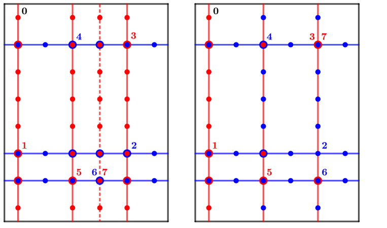
Figure 1: Both figures show an instance of the first seven steps in the BRD. The figure on the left describes the case in which $\tau^{\operatorname{\mathsf{NE}}}_{n}=6$. To compute $\operatorname{\mathsf{BRD}}_{n}(7)$, the row player visits the action profiles on the red dashed lines and finds the maximum payoff at $\operatorname{\mathsf{BRD}}_{n}(6)$; hence $\operatorname{\mathsf{BRD}}_{n}(6)\in\operatorname{\mathsf{NE}}_{n}$. In this case $R_{n}(5)$ consists of all the action profiles on the solid red and blue lines in the figure. Hence, $\tau^{R}_{n}=7$ and, consequently, $\tau^{R}_{n}-1=\tau^{\operatorname{\mathsf{NE}}}_{n}$. The figure on the right describes the case in which the BRD discovers a trap. Since $\operatorname{\mathsf{BRD}}_{n}(6)$ and $\operatorname{\mathsf{BRD}}_{n}(3)$ are in the same column, we have $\operatorname{\mathsf{BRD}}_{n}(7)=\operatorname{\mathsf{BRD}}_{n}(3)$. In this case $\tau^{R}_{n}=6$ because $R_{n}(4)$ consists of all the action profiles on the solid lines in the figure, except for the blue line passing through the action profiles labeled $5$ and $6$. Hence, $\operatorname{\mathsf{BRD}}_{n}(\tau^{R}_{n}+1)=\operatorname{\mathsf{BRD}}_{n}(t)$ for $t=3\leq\tau^{R}_{n}-3$.

In general, the trajectory of the BRD for all $t\geq 0$ is completely determined by the trajectory up to the random time $\tau_{n}^{R}$. Concerning the random time $\tau_{n}^{\operatorname{\mathsf{NE}}}$ defined in (4.2), notice that

1. in the case described in (i), we have $\tau_{n}^{\operatorname{\mathsf{NE}}}=\tau_{n}^{R}-1$ if $\tau_{n}^{R}>2$, and $\tau_{n}^{\operatorname{\mathsf{NE}}}=0$ if $\tau_{n}^{R}=2$ (see Fig. 1 on the left);

2. whereas, in the case in (ii), $\tau_{n}^{\operatorname{\mathsf{NE}}}=\infty$.

By (4.3) and (4.5), we have

$$\mathsf{P}(\tau_{n}^{R}\leq 2K_{n})=1\ ,$$ (4.6)

Moreover, by (4.6) and (a), if a PNE is eventually reached, then the BRD must visit the set $\operatorname{\mathsf{NE}}_{n}$ for the first time within $2K_{n}-1$ steps. Formally,

$$\mathsf{P}(\tau_{n}^{\operatorname{\mathsf{NE}}}\leq 2K_{n}-1)=1-\mathsf{P}(\tau_{n}^{\operatorname{\mathsf{NE}}}=\infty)\ .$$ (4.7)

As shown in the following lemma, another relevant feature of (4.3) and (4.4) is that, for all $t\geq 1$, conditionally on the event $\{\tau_{n}^{R}>t\}$, even if the set $R_{n}(t)$ is random, its cardinality $\left\lvert R_{n}(t)\right\rvert$ is almost surely equal to the deterministic value $r_{n}$.

Lemma 4.1.

Fix any $n\in\mathbb{N}$ and $p_{n}\in[0,1]$. Call, for every $t\geq 1$,

$$r_{n}(t)\coloneqq\left\lceil\dfrac{t+1}{2}\right\rceil K_{n}^{\mathrm{A}}+\left\lfloor\dfrac{t+1}{2}\right\rfloor K_{n}^{\mathrm{B}}-\left\lfloor\dfrac{t+1}{2}\right\rfloor\left\lceil\dfrac{t+1}{2}\right\rceil.$$ (4.8)

Then, for every $t\geq 1$,

$$\mathsf{P}\left(\lvert R_{n}(t)\rvert=r_{n}(t)\mid\tau_{n}^{R}>t\right)=1.$$ (4.9)

4.2 Potential games

We start studying the case of $p=1$, i.e., the case of potential games. A potential game cannot have traps. Therefore, thanks to (a),

$$\left\{\tau_{n}^{R}=t\right\}=\left\{\tau_{n}^{\operatorname{\mathsf{NE}}}=t-1\right\},\quad\text{for }t>2,$$ (4.10)

and, together with (4.7) and (4.6), we recover the well-known fact

$$\mathsf{P}(\tau_{n}^{\operatorname{\mathsf{NE}}}<\infty)=1\,,\qquad n\geq 1.$$ (4.11)

Define

$$q_{t,n} \coloneqq\mathsf{P}\left(\tau_{n}^{\operatorname{\mathsf{NE}}}=t\mid\tau_{n}^{\operatorname{\mathsf{NE}}}\geq t\right)\quad\text{for all }t\in\left\{0,\dots,2K_{n}-1\right\}.$$ (4.12)

In words, $q_{t,n}$ represents the conditional probability that a PNE is reached at time $t$, given that it was not reached before. Notice that if $t=2K_{n}-1$, then $q_{t,n}=1$. We start with a non-asymptotic result, which, for every $n\in\mathbb{N}$, provides the value of $q_{t,n}$ for all $t\leq 2K_{n}-1$.

Lemma 4.2.

Fix $n\in\mathbb{N}$, let $p_{n}=1$ and recal the definition of $r_{n}(t)$ in (4.8). Then,

$$q_{0,n} =\frac{1}{K_{n}^{\mathrm{A}}+K_{n}^{\mathrm{B}}-1},$$ (4.13)

$$q_{1,n} =\frac{K_{n}^{\mathrm{A}}-1}{K_{n}^{\mathrm{A}}+K_{n}^{\mathrm{B}}-2},$$ (4.14)

and, for $$t\geq 2$$,

$$q_{t,n} =\frac{r_{n}(t-1)}{r_{n}(t)}.$$ (4.15)

As an immediate consequence of the previous lemma, we obtain the exact form of the distribution of the random time $\tau_{n}^{\operatorname{\mathsf{NE}}}$.

Theorem 4.3.

With the definitions of Lemma 4.2, we have

$$\mathsf{P}\left(\tau_{n}^{\operatorname{\mathsf{NE}}}>t\right)=\prod_{j=0}^{t}(1-q_{j,n}).$$ (4.16)

The following proposition provides the asymptotic expectation and variance of $\tau_{n}^{\operatorname{\mathsf{NE}}}$ when the two players have the same action set.

Proposition 4.4.

If $p_{n}=1$ and $K_{n}^{\mathrm{A}}=K_{n}^{\mathrm{B}}$ for every $n\in\mathbb{N}$. Then

$$\lim_{n\to\infty}\mathsf{E}\left[\tau_{n}^{\operatorname{\mathsf{NE}}}\right] =\operatorname{e}-1$$ (4.17)

$$\lim_{n\to\infty}\operatorname{\mathsf{Var}}\left[\tau_{n}^{\operatorname{\mathsf{NE}}}\right] \approx 0.767.$$ (4.18)

We point out that our expression for $\mathsf{E}\left[\tau_{n}^{\operatorname{\mathsf{NE}}}\right]$ coincides with the one in Durand and Gaujal, (2016, theorem 4), but the proof techniques exploited in Theorem 4.3 are completely different from the ones used by Durand and Gaujal, (2016); moreover, our analysis considers the whole distribution of $\tau_{n}^{\operatorname{\mathsf{NE}}}$ and not just its expectation.

4.3 Games with i.i.d. payoffs

In a recent paper Amiet et al., 2021a (, theorem 2.3) showed that, when $p_{n}=0$ and $K_{n}^{\mathrm{A}}=K_{n}^{\mathrm{B}}$, with high probability as $n\to\infty$, the BRD does not converge to the set $\operatorname{\mathsf{NE}}_{n}$. We start by generalizing their result to the general setting $K_{n}^{\mathrm{A}}\neq K_{n}^{\mathrm{B}}$.

Theorem 4.5.

Let $p_{n}=0$ for all $n\in\mathbb{N}$. Then

$$\lim_{n\to\infty}\mathsf{P}(\tau_{n}^{\operatorname{\mathsf{NE}}}<\infty)=0.$$ (4.19)

Even though the result in Theorem 4.5 can be achieved by naturally adapting the proof of Amiet et al., 2021a (, theorem 2.3) to the rectangular case, for completeness we present a detailed proof in Section 5. It is worth stressing that, contrarily to our setting, Amiet et al., 2021a assume that the BRD starts at an action profile in which the second player is already at best-response. The fact that we dispense with this assumption makes the quantities appearing in our proof slightly different from those in Amiet et al., 2021a .

4.4 The general case

The main purpose of this paper is to complement the negative result in Theorem 4.5 by showing that a tiny bit of (positive) correlation in the players payoffs, namely $p_{n}>0$, is enough to dramatically change the picture and make it similar to the case of a potential game, i.e., $p_{n}=1$.

More precisely, the following result shows that, if $p_{n}$ is not too small compared to $K_{n}$, then the probability of the event $\left\{\tau_{n}^{\operatorname{\mathsf{NE}}}=\infty\right\}$ vanishes as $n$ goes to infinity.

Theorem 4.6.

Fix a positive sequence $p_{n}$. If

$$\lim_{n\to\infty}\frac{\log(p_{n})}{\log(K_{n})}=0,$$ (4.20)

then

$$\lim_{n\to\infty}\mathsf{P}\left(\tau_{n}^{\operatorname{\mathsf{NE}}}=\infty\right)=0.$$ (4.21)

Notice that the latter result is qualitative in nature: it tells us that the BRD will eventually converge to a Nash equilibrium rather than to a trap, but does not provide any bound on the rate of convergence beyond the trivial one presented in (4.7). The following result—which implies Theorem 4.6—provides a much better bound on the time of convergence. Indeed, it states that, under the condition in (4.20), the time of convergence of the BRD to an equilibrium can be upper bounded, with high probability, by any function diverging exponentially faster than $p_{n}^{-1}$.

Proposition 4.7.

Fix a positive sequence $p_{n}$ satisfying (4.20). Then, for any sequence $\ell_{n}$ such that

$$\lim_{n\rightarrow\infty}\ell_{n}=\infty\quad\text{and}\quad\lim_{n\rightarrow\infty}\frac{\log(p_{n})}{\log(\ell_{n})}=0,$$ (4.22)

we have

$$\lim_{n\to\infty}\mathsf{P}\left(\tau_{n}^{\operatorname{\mathsf{NE}}}>\ell_{n}\right)=0\,.$$ (4.23)

Notice that Theorem 4.6 follows from Proposition 4.7 by choosing $\ell_{n}=2K_{n}-1$. In the particular case when $p_{n}=p>0$ for all $n\in\mathbb{N}$, Proposition 4.7 states that, with high probability, a PNE is reached by the BRD in at most $\ell_{n}$ steps, no matter how slowly the sequence $\ell_{n}$ diverges.

Remark 4.8.

Notice that, whenever $p_{n}<1$, the random variable $\tau_{n}^{\operatorname{\mathsf{NE}}}$ takes value $+\infty$ with positive probability. Therefore, even though (4.21) holds true, the random variable $\tau_{n}^{\operatorname{\mathsf{NE}}}$ cannot have a finite expectation.

5 Proofs

Proofs of Section 3

Proof of Proposition 3.1.

By linearity of expectation, we have

$$\mathsf{E}\left[W\right]=K^{\mathrm{A}}K^{\mathrm{B}}\mathsf{P}((1,1)\in\operatorname{\mathsf{NE}}).$$ (5.1)

Conditioning on the event $\left\{U^{\mathrm{A}}(1,1)=U^{\mathrm{B}}(1,1)\right\}$ and using the law of total probability, we get

$$\mathsf{P}((1,1)\in\operatorname{\mathsf{NE}})=p\frac{1}{K^{\mathrm{A}}+K^{\mathrm{B}}-1}+(1-p)\frac{1}{K^{\mathrm{A}}K^{\mathrm{B}}}.$$ (5.2)

To see that (5.2) holds, consider the following: when $U^{\mathrm{A}}(1,1)=U^{\mathrm{B}}(1,1)$, the profile $(1,1)$ is a PNE if and only if $U^{\mathrm{A}}(1,1)$ is larger than or equal to all payoffs $U^{\mathrm{A}}(a,1)$ and all payoffs $U^{\mathrm{B}}(1,b)$ for all $a\in[K^{\mathrm{A}}]$ and all $b\in[K^{\mathrm{B}}]$. By symmetry, this happens with probability $1/(K^{\mathrm{A}}+K^{\mathrm{B}}-1)$. On the other hand, when $U^{\mathrm{A}}(1,1)\neq U^{\mathrm{B}}(1,1)$, the profile $(1,1)$ is a PNE if and only if $U^{\mathrm{A}}(1,1)$ is larger than or equal to all payoffs $U^{\mathrm{A}}(a,1)$ for all $a\in[K^{\mathrm{A}}]$ and $U^{\mathrm{B}}(1,1)$ is larger than or equal to all payoffs $U^{\mathrm{B}}(1,b)$ for all $b\in[K^{\mathrm{B}}]$. By independence of the payoffs and by symmetry, this happens with probability $1/K^{\mathrm{A}}K^{\mathrm{B}}$. Plugging (5.2) into (5.1), we get the result. ∎

Proof of Proposition 3.2.

By Proposition 3.1 we get

$$\mathsf{E}\left[W_{n}\right]=p_{n}\frac{K_{n}^{\mathrm{A}}K_{n}^{\mathrm{B}}}{K_{n}^{\mathrm{A}}+K_{n}^{\mathrm{B}}-1}+(1-p_{n})=(1+o(1))p_{n}\frac{K_{n}^{\mathrm{A}}K_{n}^{\mathrm{B}}}{K_{n}^{\mathrm{A}}+K_{n}^{\mathrm{B}}},$$ (5.3)

where, in the asymptotic equality we used the fact that $p_{n}K_{n}\to\infty$. This shows that $\mathsf{E}\left[W_{n}\right]\to\infty$.

We now show that $W_{n}$ concentrates around its expectation. To this end, we use an upper bound on the second moment of $W_{n}$. Notice that

$$\begin{split}\mathsf{E}\left[W_{n}^{2}\right]&=\mathsf{E}\left[\left(\sum_{(a,b)\in[K_{n}^{\mathrm{A}}]\times[K_{n}^{\mathrm{B}}]}\mathds{1}_{(a,b)\in\operatorname{\mathsf{NE}}_{n}}\right)^{2}\right]\\ &=\sum_{(a,b)\in[K_{n}^{\mathrm{A}}]\times[K_{n}^{\mathrm{B}}]}\sum_{(a^{\prime},b^{\prime})\in[K_{n}^{\mathrm{A}}]\times[K_{n}^{\mathrm{B}}]}\mathsf{P}\left((a,b),(a^{\prime},b^{\prime})\in\operatorname{\mathsf{NE}}_{n}\right).\end{split}$$ (5.4)

From (5.4) it follows immediately that the computation of the second moment amounts to studying probabilities of the form

$$\mathsf{P}\left((a,b),(a^{\prime},b^{\prime})\in\operatorname{\mathsf{NE}}_{n}\right)\ ,\qquad a,a^{\prime}\in[K_{n}^{\mathrm{A}}],\>b,b^{\prime}\in[K_{n}^{\mathrm{B}}].$$

We argue that there are only three relevant cases:

1. $a=a^{\prime}$ and $b=b^{\prime}$;

2. $a=a^{\prime}$ and $b\neq b^{\prime}$ or vice versa;

3. $a\neq a^{\prime}$ and $b\neq b^{\prime}$;

Case (a) is trivial:

$$\mathsf{P}\left((a,b),(a^{\prime},b^{\prime})\in\operatorname{\mathsf{NE}}_{n}\right)=\mathsf{P}\left((a,b)\in\operatorname{\mathsf{NE}}_{n}\right)\ .$$ (5.5)

The continuity of $F$ implies that in Case (b) we have

$$\mathsf{P}\left((a,b),(a^{\prime},b^{\prime})\in\operatorname{\mathsf{NE}}_{n}\right)=0.$$ (5.6)

To analyze Case (c), we remark that, if $a\neq a^{\prime}$ and $b\neq b^{\prime}$, then the event $\left\{(a^{\prime},b^{\prime})\in\operatorname{\mathsf{NE}}_{n}\right\}$ depends on the event $\left\{(a,b)\in\operatorname{\mathsf{NE}}_{n}\right\}$ only through the payoffs $U^{\mathrm{A}}(a^{\prime},b)$ and $U^{\mathrm{B}}(a,b^{\prime})$. Therefore

$$\begin{split}\mathsf{P}\left((a,b),(a^{\prime},b^{\prime})\in\operatorname{\mathsf{NE}}_{n}\right)&=\mathsf{P}\left((a,b)\in\operatorname{\mathsf{NE}}_{n}\right)\mathsf{P}\left((a^{\prime},b^{\prime})\in\operatorname{\mathsf{NE}}_{n}\mid(a,b)\in\operatorname{\mathsf{NE}}_{n}\right)\\ &\leq\mathsf{P}\left((a,b)\in\operatorname{\mathsf{NE}}_{n}\right)\mathsf{P}\left(U^{\mathrm{A}}(a^{\prime},b^{\prime})=\max_{a^{\prime\prime}\in\left[K_{n}^{\mathrm{A}}\right]\setminus\{a\}}U^{\mathrm{A}}(a^{\prime\prime},b^{\prime}),\right.\\ &\left.\qquad U^{\mathrm{B}}(a^{\prime},b^{\prime})=\max_{b^{\prime\prime}\in[K_{n}^{\mathrm{B}}]\setminus\{b\}}U^{\mathrm{B}}(a^{\prime},b^{\prime\prime})\right)\\ &=\mathsf{P}\left((a,b)\in\operatorname{\mathsf{NE}}_{n}\right)\left(p_{n}\frac{1}{K_{n}^{\mathrm{A}}+K_{n}^{\mathrm{B}}-3}+(1-p_{n})\frac{1}{(K_{n}^{\mathrm{A}}-1)(K_{n}^{\mathrm{B}}-1)}\right)\\ &=(1+o(1))\left(\mathsf{P}\left((a,b)\in\operatorname{\mathsf{NE}}_{n}\right)\right)^{2}.\end{split}$$ (5.7)

The inequality in (5.7) stems from the fact that the event $(a^{\prime},b^{\prime})\in\operatorname{\mathsf{NE}}_{n}$ coincides with the event $\left\{U^{\mathrm{A}}(a^{\prime},b^{\prime})=\max_{a^{\prime\prime}\in\left[K_{n}^{\mathrm{A}}\right]}U^{\mathrm{A}}(a^{\prime\prime},b^{\prime}),\,U^{\mathrm{B}}(a^{\prime},b^{\prime})=\max_{b^{\prime\prime}\in[K_{n}^{\mathrm{B}}]}U^{\mathrm{B}}(a^{\prime},b^{\prime\prime})\right\}$, which in turn implies the event $\left\{U^{\mathrm{A}}(a^{\prime},b^{\prime})=\max_{a^{\prime\prime}\in\left[K_{n}^{\mathrm{A}}\right]\setminus\{a\}}U^{\mathrm{A}}(a^{\prime\prime},b^{\prime}),\,U^{\mathrm{B}}(a^{\prime},b^{\prime})=\max_{b^{\prime\prime}\in[K_{n}^{\mathrm{B}}]\setminus\{b\}}U^{\mathrm{B}}(a^{\prime},b^{\prime\prime})\right\}$. The independence between this latter event and $\{(a,b)\in\operatorname{\mathsf{NE}}_{n}\}$ proves the inequality. The second equality in (5.7), follows from the fact that, when $U^{\mathrm{A}}(a^{\prime},b^{\prime})=U^{\mathrm{B}}(a^{\prime},b^{\prime})$, which happens with probability $p_{n}$, the event

$$\left\{U^{\mathrm{A}}(a^{\prime},b^{\prime})=\max_{a^{\prime\prime}\in[K_{n}^{\mathrm{A}}]\setminus\{a\}}U^{\mathrm{A}}(a^{\prime\prime},b^{\prime})\,,\,U^{\mathrm{B}}(a^{\prime},b^{\prime})=\max_{b^{\prime\prime}\in[K_{n}^{\mathrm{B}}]\setminus\{b\}}U^{\mathrm{B}}(a^{\prime},b^{\prime\prime})\right\}$$ (5.8)

has the same probability as the event of picking the maximum among $K_{n}^{\mathrm{A}}+K_{n}^{\mathrm{B}}-3$ equally probable objects; on the other hand, when $U^{\mathrm{A}}(a^{\prime},b^{\prime})\neq U^{\mathrm{B}}(a^{\prime},b^{\prime})$, the event in (5.8) has the same probability of picking independently the maximum of $K_{n}^{\mathrm{A}}-1$ equally probably objects and the maximum of $K_{n}^{\mathrm{B}}-1$ equally probably objects. The last equality stems from (5.2).

In conclusion, plugging Eqs. 5.5, 5.6 and 5.7 into (5.4), we obtain

$$\begin{split}\mathsf{E}\left[W_{n}^{2}\right]&=\sum_{(a,b)\in[K_{n}^{\mathrm{A}}]\times[K_{n}^{\mathrm{B}}]}\mathsf{P}\left((a,b)\in\operatorname{\mathsf{NE}}_{n}\right)\\ &\quad+(1+o(1))\sum_{(a,b)\in[K_{n}^{\mathrm{A}}]\times[K_{n}^{\mathrm{B}}]}\sum_{\begin{subarray}{c}(a^{\prime},b^{\prime})\in[K_{n}^{\mathrm{A}}]\times[K_{n}^{\mathrm{B}}]\\ a\neq a^{\prime},b\neq b^{\prime}\end{subarray}}\left(\mathsf{P}\left((a,b)\in\operatorname{\mathsf{NE}}_{n}\right)\right)^{2}\\ &<\mathsf{E}\left[W_{n}\right]+(1+o(1))(\mathsf{E}\left[W_{n}\right])^{2}\\ &=(1+o(1))(\mathsf{E}\left[W_{n}\right])^{2},\end{split}$$ (5.9)

where the last equality stems from the fact that $\mathsf{E}\left[W_{n}\right]\to\infty$, which implies $\mathsf{E}\left[W_{n}\right]=o((\mathsf{E}\left[W_{n}\right])^{2})$.

By Chebyshev’s inequality, we have that, for every $\varepsilon>0$,

$$\mathsf{P}\left(\left\lvert W_{n}-\mathsf{E}[W_{n}]\right\rvert\geq\varepsilon\mathsf{E}[W_{n}]\right)\leq\frac{\mathsf{E}\left[W_{n}^{2}\right]-\left(\mathsf{E}\left[W_{n}\right]\right)^{2}}{\varepsilon^{2}\left(\mathsf{E}\left[W_{n}\right]\right)^{2}}=o(1),$$ (5.10)

where the asymptotic upper bound follows from (5.9). ∎

Proofs of Section 4.1

Proof of Lemma 4.1.

We prove (4.9) by induction. For $t=1$ we have $\lvert R_{n}(1)\rvert=K_{n}^{\mathrm{A}}+K_{n}^{\mathrm{B}}-1$, which is trivially true. Assume now that (4.9) holds up to $t-1<\tau_{n}^{R}$. Notice that, conditioning on $\{\tau_{n}^{R}>t\}$, $\operatorname{\mathsf{BRD}}_{n}(t)$ cannot visit a row or column visited at time $1,2,\ldots,t-1$. Since player $\mathrm{A}$ plays first, by the inductive hypothesis and thanks to the conditioning, for $0<t<\tau_{n}^{R}$, we have almost surely,

$$\lvert R_{n}(t)\rvert=\begin{cases}r_{n}(t-1)+K_{n}^{\mathrm{B}}-\left\lfloor\dfrac{t+1}{2}\right\rfloor\,,&\text{if $t$ is odd};\\ \\ r_{n}(t-1)+K_{n}^{\mathrm{A}}-\left\lfloor\dfrac{t+1}{2}\right\rfloor\,,&\text{if $t$ is even}.\end{cases}$$ (5.11)

Since

$$r_{n}(t-1)=\left\lceil\dfrac{t}{2}\right\rceil K_{n}^{\mathrm{A}}+\left\lfloor\dfrac{t}{2}\right\rfloor K_{n}^{\mathrm{B}}-\left\lfloor\dfrac{t}{2}\right\rfloor\left\lceil\dfrac{t}{2}\right\rceil,$$ (5.12)

we can rewrite the right hand side of (5.11) as (4.8). Hence, (4.9) holds. ∎

Proofs of Section 4.2

Proof of Lemma 4.2.

Since $p_{n}=1$, we have $\boldsymbol{U}_{n}^{\mathrm{A}}=\boldsymbol{U}_{n}^{\mathrm{B}}$ almost surely. Therefore, to simplify the notation, we write

$$U_{n}(a,b)\coloneqq U^{\mathrm{A}}_{n}(a,b)=U^{\mathrm{B}}_{n}(a,b).$$ (5.13)

Moreover, in a potential game $\left\{\tau_{n}^{R}=t\right\}=\left\{\tau_{n}^{\operatorname{\mathsf{NE}}}=t-1\right\}$, for $t>2$, as in (4.10). We start with $t=0$. We have

$$\begin{split}q_{0,n}&=\mathsf{P}\left(\tau_{n}^{\operatorname{\mathsf{NE}}}=0\right)\\ &=\mathsf{P}\left(U_{n}(1,1)=\max\left\{\max_{a\in[K_{n}^{\mathrm{A}}]}U_{n}(a,1),\max_{b\in[K_{n}^{\mathrm{B}}]}U_{n}(1,b)\right\}\right)\\ &=\frac{1}{K_{n}^{\mathrm{A}}+K_{n}^{\mathrm{B}}-1}.\end{split}$$ (5.14)

Let now $t=1$. We have

$$\mathsf{P}\left(\tau_{n}^{\operatorname{\mathsf{NE}}}\geq 1\right)=\mathsf{P}\left(\tau_{n}^{\operatorname{\mathsf{NE}}}\geq 0\right)-\mathsf{P}\left(\tau_{n}^{\operatorname{\mathsf{NE}}}=0\right)=1-\frac{1}{K_{n}^{\mathrm{A}}+K_{n}^{\mathrm{B}}-1}=\frac{K_{n}^{\mathrm{A}}+K_{n}^{\mathrm{B}}-2}{K_{n}^{\mathrm{A}}+K_{n}^{\mathrm{B}}-1}.$$ (5.15)

Moreover, if we define the event

$$A_{a}\coloneqq\left\{\text{player $\mathrm{A}$'s best response to action $1$ is $a$}\right\},$$ (5.16)

we have

$$\begin{split}\mathsf{P}\left(\tau_{n}^{\operatorname{\mathsf{NE}}}=1\right)&=\sum_{a\in[K_{n}^{\mathrm{A}}]}\mathsf{P}\left(\tau_{n}^{\operatorname{\mathsf{NE}}}=1\mid A_{a}\right)\mathsf{P}(A_{a})\\ &=\sum_{a=2}^{K_{n}^{\mathrm{A}}}\mathsf{P}\left(\operatorname{\mathsf{Beta}}\left(K_{n}^{\mathrm{A}},1\right)\geq\operatorname{\mathsf{Beta}}\left(K_{n}^{\mathrm{B}}-1,1\right)\right)\frac{1}{K_{n}^{\mathrm{A}}}\\ &=\sum_{a=2}^{K_{n}^{\mathrm{A}}}\frac{K_{n}^{\mathrm{A}}}{K_{n}^{\mathrm{A}}+K_{n}^{\mathrm{B}}-1}\cdot\frac{1}{K_{n}^{\mathrm{A}}}\\ &=\frac{K_{n}^{\mathrm{A}}-1}{K_{n}^{\mathrm{A}}+K_{n}^{\mathrm{B}}-1},\end{split}$$ (5.17)

where, with an abuse of notation, we have identified a random variable with its distribution. Conditionally on $A_{a}$, we have $\tau_{n}^{\operatorname{\mathsf{NE}}}=1$ if the payoff in $(a,1)$ is the largest among all payoffs in the same row. To get the result we have applied Proposition B.1 about the maximum of uniform independent random variables and Proposition B.2 about the probability that a $\operatorname{\mathsf{Beta}}(a,1)$ is larger than an independent $\operatorname{\mathsf{Beta}}(b,1)$. This result can be applied because the payoffs, and consequently the two Beta random variables, are independent. Therefore, combining (5.15) and (5.17), we obtain

$$\begin{split}q_{1,n}&=\mathsf{P}\left(\tau_{n}^{\operatorname{\mathsf{NE}}}=1\mid\tau_{n}^{\operatorname{\mathsf{NE}}}\geq 1\right)\\ &=\frac{\mathsf{P}\left(\tau_{n}^{\operatorname{\mathsf{NE}}}=1\right)}{\mathsf{P}\left(\tau_{n}^{\operatorname{\mathsf{NE}}}\geq 1\right)}\\ &=\frac{K_{n}^{\mathrm{A}}+K_{n}^{\mathrm{B}}-1}{K_{n}^{\mathrm{A}}+K_{n}^{\mathrm{B}}-2}\cdot\frac{K_{n}^{\mathrm{A}}-1}{K_{n}^{\mathrm{A}}+K_{n}^{\mathrm{B}}-1}\\ &=\frac{K_{n}^{\mathrm{A}}-1}{K_{n}^{\mathrm{A}}+K_{n}^{\mathrm{B}}-2}.\end{split}$$ (5.18)

Let now $t\geq 2$. Call $\Pi_{t}$ the set of sequences $\pi=(\pi_{0},\pi_{1},\ldots,\pi_{t})$ such that

• $\pi_{i}=(a_{i},b_{i})\in[K_{n}^{\mathrm{A}}]\times[K_{n}^{\mathrm{B}}]$ for $i\geq 0$,

• $\pi_{0}=(1,1)$,

• if $i$ is odd, then $b_{i}=b_{i-1}$, whereas, if $i>0$ is even, then $a_{i}=a_{i-1}$,

• there is no pair of distinct odd indices $i,j$ such that $b_{i}=b_{j}$,

• there is no pair of distinct even indices $i,j$ such that $a_{i}=a_{j}$.

Notice that the set $\Pi_{t}$ coincides with all possible trajectories of length $t$ of $\operatorname{\mathsf{BRD}}_{n}$ satisfying the event $\left\{\tau_{n}^{\operatorname{\mathsf{NE}}}\geq t\right\}$. Define the event

$$G_{t}^{\pi}=\left\{\operatorname{\mathsf{BRD}}_{n}(s)=\pi_{s}\text{ for }0\leq s\leq t\right\}.$$ (5.19)

Notice that

$$q_{t,n}\coloneqq\mathsf{P}\left(\tau_{n}^{\operatorname{\mathsf{NE}}}=t\mid\tau_{n}^{\operatorname{\mathsf{NE}}}\geq t\right)=\sum_{\pi\in\Pi_{t}}\mathsf{P}\left(\tau_{n}^{\operatorname{\mathsf{NE}}}=t\mid G_{t}^{\pi},\,\tau_{n}^{\operatorname{\mathsf{NE}}}\geq t\right)\mathsf{P}\left(G_{t}^{\pi}\mid\tau_{n}^{\operatorname{\mathsf{NE}}}\geq t\right).$$ (5.20)

The conditional probability $\mathsf{P}\left(\tau_{n}^{\operatorname{\mathsf{NE}}}=t\mid G_{t}^{\pi},\,\tau_{n}^{\operatorname{\mathsf{NE}}}\geq t\right)$ equals the probability that the maximum of $r_{n}(t-1)$ i.i.d. uniform random variables is bigger than the maximum of $K^{\ast}_{n}-\left\lfloor\frac{t+1}{2}\right\rfloor$ uniform random variables, where

$$K^{\ast}_{n}=\begin{cases}K_{n}^{\mathrm{A}}&\text{if $t$ is even,}\\ K_{n}^{\mathrm{B}}&\text{if $t$ is odd.}\end{cases}$$ (5.21)

The conditioning event $G_{t}^{\pi}\cap\{\tau_{n}^{\operatorname{\mathsf{NE}}}\geq t\}$ determines the position of $\operatorname{\mathsf{BRD}}_{n}(t)$ and the fact that the payoffs associated to $r_{n}(t-1)$ action profiles up to time $t$ have been computed by the BRD. The payoff associated to $\operatorname{\mathsf{BRD}}_{n}(t)$ is the maximum of $r_{n}(t-1)$ i.i.d. uniform random variables. The probability that the action profile $\operatorname{\mathsf{BRD}}_{n}(t)$ is a PNE is the probability that its payoff is larger than all the previously uncomputed payoffs associated to action profiles in its same column (if $t$ is even) or in its same row (if $t$ is odd). This requires a comparison with $K^{\ast}_{n}-\left\lfloor\frac{t+1}{2}\right\rfloor$ uniformly distributed payoffs. So

$$\mathsf{P}\left(\tau_{n}^{\operatorname{\mathsf{NE}}}=t\mid G_{t}^{\pi},\,\tau_{n}^{\operatorname{\mathsf{NE}}}\geq t\right) =\mathsf{P}\left(\operatorname{\mathsf{Beta}}(r_{n}(t-1),1)>\operatorname{\mathsf{Beta}}\left(K^{\ast}_{n}-\left\lfloor\frac{t+1}{2}\right\rfloor,1\right)\right)$$

$$=\frac{r_{n}(t-1)}{r_{n}(t-1)+K^{\ast}_{n}-\left\lfloor\frac{t+1}{2}\right\rfloor}$$

$$=\frac{r_{n}(t-1)}{r_{n}(t)}\,,$$

where the last identity is due to (5.11). Using (5.20) we get

$$\begin{split}\mathsf{P}\left(\tau_{n}^{\operatorname{\mathsf{NE}}}=t\mid\tau_{n}^{\operatorname{\mathsf{NE}}}\geq t\right)&=\sum_{\pi\in\Pi_{t}}\mathsf{P}\left(\tau_{n}^{\operatorname{\mathsf{NE}}}=t\mid G_{t}^{\pi},\,\tau_{n}^{\operatorname{\mathsf{NE}}}\geq t\right)\mathsf{P}\left(G_{t}^{\pi}\mid\tau_{n}^{\operatorname{\mathsf{NE}}}\geq t\right)\\ &=\frac{r_{n}(t-1)}{r_{n}(t)}\sum_{\pi\in\Pi_{t}}\mathsf{P}\left(G_{t}^{\pi}\mid\tau_{n}^{\operatorname{\mathsf{NE}}}\geq t\right)\,.\end{split}$$ (5.22)

Note that $\{\tau_{n}^{\operatorname{\mathsf{NE}}}\geq t\}=\sqcup_{\pi\in\Pi_{t}}G_{t}^{\pi}$. Hence

$$\sum_{\pi\in\Pi_{t}}\mathsf{P}\left(G_{t}^{\pi}\mid\tau_{n}^{\operatorname{\mathsf{NE}}}\geq t\right)=\mathsf{P}\left(\tau_{n}^{\operatorname{\mathsf{NE}}}\geq t\mid\tau_{n}^{\operatorname{\mathsf{NE}}}\geq t\right)=1\,.$$ (5.23)

Therefore, (5.22) becomes

$$\mathsf{P}\left(\tau_{n}^{\operatorname{\mathsf{NE}}}=t\mid\tau_{n}^{\operatorname{\mathsf{NE}}}\geq t\right)=\frac{r_{n}(t-1)}{r_{n}(t)}\,.\qed$$

Proof of Theorem 4.3.

Note that

$$\mathsf{P}\left(\tau_{n}^{\operatorname{\mathsf{NE}}}>t\right)=\mathsf{P}\left(\tau_{n}^{\operatorname{\mathsf{NE}}}>t\mid\tau_{n}^{\operatorname{\mathsf{NE}}}>t-1\right)\mathsf{P}\left(\tau_{n}^{\operatorname{\mathsf{NE}}}>t-1\right)=(1-q_{t,n})\mathsf{P}\left(\tau_{n}^{\operatorname{\mathsf{NE}}}>t-1\right)\,.$$ (5.24)

Hence, by iteration, we get

$$\mathsf{P}\left(\tau_{n}^{\operatorname{\mathsf{NE}}}>t\right)=\prod_{j=1}^{t}(1-q_{j,n})\cdot\mathsf{P}\left(\tau_{n}^{\operatorname{\mathsf{NE}}}>0\right)=\prod_{j=0}^{t}(1-q_{j,n})\,.\qed$$

Proof of Proposition 4.4.

We first compute $\mathsf{E}\left[\tau_{n}^{\operatorname{\mathsf{NE}}}\right]$. By Theorem 4.3 we have

$$\mathsf{E}\left[\tau_{n}^{\operatorname{\mathsf{NE}}}\right]=\sum_{t=0}^{2K_{n}-2}\mathsf{P}\left(\tau_{n}^{\operatorname{\mathsf{NE}}}>t\right)=\sum_{t=0}^{2K_{n}-2}\prod_{j=0}^{t}(1-q_{j,n})\,.$$ (5.25)

We split the first sum in (5.25) into two parts: $t\in\left\{0,\dots,\ell_{n}-1\right\}$ and $t\in\left\{\ell_{n},\dots,2K_{n}-2\right\}$, where $\ell_{n}=\lfloor\left(\log K_{n}\right)^{2}\rfloor$. We start by showing that

$$\lim_{n\to\infty}\sum_{t=\ell_{n}}^{2K_{n}-2}\prod_{j=0}^{t}(1-q_{j,n})=0,$$ (5.26)

for which it suffices to show that for $t\geq\ell_{n}$

$$\mathsf{P}(\tau_{n}^{\operatorname{\mathsf{NE}}}>t)=\prod_{j=0}^{t}(1-q_{j,n})=o\left(K_{n}^{-1}\right).$$ (5.27)

Notice that the sequence $q_{t,n}$, defined in (4.12), is increasing in $t$. Hence, for $t\geq\ell_{n}$, we have

$$\mathsf{P}\left(\tau_{n}^{\operatorname{\mathsf{NE}}}>t\right)\leq(1-q_{0,n})(1-q_{1,n})^{\ell_{n}}\leq\frac{1}{2^{\ell_{n}}}=o\left(K_{n}^{-1}\right)\,,$$ (5.28)

where in the last asymptotic equality we used $q_{1,n}=1/2$ and $\ell_{n}=\omega(\log(K_{n}))$.

We are left to show that

$$\lim_{n\to\infty}\sum_{t=0}^{\ell_{n}}\prod_{j=0}^{t}(1-q_{j,n})=\operatorname{e}-1\,.$$ (5.29)

Notice that

$$1-q_{0,n}=\frac{2K_{n}-2}{2K_{n}-1}=1-\mathcal{O}\left(K_{n}^{-1}\right)\quad\text{and}\quad 1-q_{1,n}=\frac{1}{2}\,.$$ (5.30)

Moreover, since

$$r_{n}(t)-r_{n}(t-1)=K_{n}-\left\lceil\frac{t}{2}\right\rceil\,,$$ (5.31)

we have, for all $t\leq\ell_{n}$,

$$\begin{split}1-q_{t,n}&=\frac{r_{n}(t)-r_{n}(t-1)}{r_{n}(t)}\\ &=\frac{K_{n}-\left\lceil\frac{t}{2}\right\rceil}{(t+1)K_{n}-\left\lceil\frac{t+1}{2}\right\rceil\left\lfloor\frac{t+1}{2}\right\rfloor}\\ &=\frac{1}{t+1}\cdot\frac{1-\Theta(t/K_{n})}{1-\Theta(t/K_{n})}\\ &=\frac{1}{t+1}\cdot\left(1+\mathcal{O}\left(\frac{\ell_{n}}{K_{n}}\right)\right).\end{split}$$ (5.32)

Hence, by (5.30) and (5.32), for all $t\leq\ell_{n}$,

$$\begin{split}\prod_{j=0}^{t}(1-q_{j,n})=&(1+o(1))\cdot 1\cdot\frac{1}{2}\cdot\prod_{j=2}^{t}\left[\frac{1}{j+1}\cdot\left(1+\mathcal{O}\left(\frac{\ell_{n}}{K_{n}}\right)\right)\right]\\ =&\frac{1}{(t+1)!}\left(1+\mathcal{O}\left(\frac{\ell_{n}^{2}}{K_{n}}\right)\right)\\ =&(1+o(1))\frac{1}{(t+1)!},\end{split}$$ (5.33)

where in the last two steps we used that, by definition, $\ell_{n}=o(\sqrt{K_{n}})$. Hence

$$\left(1+\mathcal{O}\left(\frac{\ell_{n}}{K_{n}}\right)\right)^{t-1}\leq\left(1+\mathcal{O}\left(\frac{\ell_{n}}{K_{n}}\right)\right)^{\ell_{n}}\leq\left(1+\mathcal{O}\left(\frac{\ell_{n}^{2}}{K_{n}}\right)\right)=(1+o(1)),\qquad 2\leq t\leq\ell_{n}.$$ (5.34)

Notice that (5.33) implies

$$\sum_{t=0}^{\ell_{n}}\prod_{j=0}^{t}(1-q_{j,n})=(1+o(1))\sum_{t=0}^{\ell_{n}}\frac{1}{(t+1)!}=(1+o(1))(\operatorname{e}-1)\,,$$ (5.35)

and (5.29) follows by taking the limit as $n\to\infty$. At this point (4.17) follows from (5.26) and (5.29).

We now prove (4.18). Call $H_{n}$ the distribution function of $\tau_{n}^{\operatorname{\mathsf{NE}}}$. By (5.33), we have, for $t\leq\ell_{n}$,

$$H_{n}(t)=1-\mathsf{P}\left(\tau_{n}^{\operatorname{\mathsf{NE}}}>t\right)=(1+o(1))\cdot\left(1-\frac{1}{(t+1)!}\right).$$ (5.36)

In what follows, we will use the following lemma, whose proof can be found, for instance, in Ogryczak and Ruszczyński, (1999, corollary 3).

Lemma 5.1.

Let $X$ be a random variable with finite expectation $\mu$, finite variance, and distribution function $G$. Define the function $\Phi(x)\coloneqq\int_{0}^{x}G(t)\ \textup{d}t$. Then

$$\frac{1}{2}\operatorname{\mathsf{Var}}[X]=\int_{0}^{+\infty}(\Phi(t)-[t-\mu]_{+})\ \textup{d}t,$$ (5.37)

where $[t-\mu]_{+}=\max\{t-\mu,0\}$.

We now go back to the proof of (4.18). Since the random variable $\tau_{n}^{\operatorname{\mathsf{NE}}}$ is bounded, we can apply Lemma 5.1 to get

$$\operatorname{\mathsf{Var}}\left[\tau_{n}^{\operatorname{\mathsf{NE}}}\right]=2\int_{0}^{\mu}\Phi_{n}(t)\ \textup{d}t+2\int_{\mu}^{+\infty}[\Phi_{n}(t)-(t-\mu)]\ \textup{d}t\,,$$ (5.38)

where, thanks to (5.36), for all $t\leq\ell_{n}$,

$$\Phi_{n}(t)=\int_{0}^{t}H_{n}(s)\ \textup{d}s\sim\int_{0}^{t}\left(1-\frac{1}{\lfloor s+1\rfloor!}\right)\ \textup{d}s,$$ (5.39)

By explicit numerical integration, using (5.39) and the fact that $\mu\coloneqq\mathsf{E}\left[\tau_{n}^{\operatorname{\mathsf{NE}}}\right]\sim\operatorname{e}-1\leq\ell_{n}$ for all $n$ sufficiently large, we get

$$2\int_{0}^{\mu}\Phi_{n}(t)\ \textup{d}t\sim 2\int_{0}^{\mu}\ \textup{d}t\int_{0}^{t}\left(1-\frac{1}{\lfloor s+1\rfloor!}\right)\ \textup{d}s\approx 0.258\,.$$ (5.40)

Moreover, for all $t\geq 0$,

$$\begin{split}\Phi_{n}(t)-(t-\mu)&=\int_{0}^{t}(H_{n}(s)-1)\ \textup{d}s+\int_{0}^{+\infty}(1-H_{n}(s))\ \textup{d}s\\ &=\int_{t}^{+\infty}(1-H_{n}(s))\ \textup{d}s\\ &=\int_{t}^{\ell_{n}\vee t}(1-H_{n}(s))\ \textup{d}s+\int_{\ell_{n}\vee t}^{+\infty}(1-H_{n}(s))\ \textup{d}s\,.\end{split}$$ (5.41)

Since the sequence $q_{t,n}$, defined in (4.12), is increasing in $t$ and $q_{1,n}=1/2$, by (5.27) we get, for all $s\geq 0$

$$1-H_{n}(s)=\mathsf{P}\left(\tau_{n}^{\operatorname{\mathsf{NE}}}>s\right)\leq\frac{1}{2^{s}}.$$ (5.42)

Hence, for all $t\geq 0$,

$$\int_{\ell_{n}\vee t}^{+\infty}(1-H_{n}(s))\ \textup{d}s\leq\frac{1}{\log 2}{2^{-(\ell_{n}\vee t)}},$$ (5.43)

which goes to zero when $n\rightarrow\infty$. Therefore, by (5.36), (5.41), and (5.43), we conclude that

$$\Phi_{n}(t)-(t-\mu)=\begin{cases}(1+o(1))\int_{t}^{\ell_{n}}\frac{1}{\lfloor s+1\rfloor!}\ \textup{d}s+\mathcal{O}(2^{-\ell_{n}})&\text{if }t\leq\ell_{n},\\ \mathcal{O}(2^{-t})&\text{if }t>\ell_{n}.\end{cases}$$ (5.44)

It is now convenient to split the second integral in (5.38) as follows

$$\begin{split}2\int_{\mu}^{+\infty}[\Phi_{n}(t)-(t-\mu)]\ \textup{d}t&=2\int_{\mu}^{\ell_{n}}[\Phi_{n}(t)-(t-\mu)]\ \textup{d}t+2\int_{\ell_{n}}^{+\infty}[\Phi_{n}(t)-(t-\mu)]\ \textup{d}t.\end{split}$$ (5.45)

At this point, using (5.44), we can bound the second integral on the right hand side of (5.45) as follows

$$\begin{split}\int_{\ell_{n}}^{\infty}[\Phi_{n}(t)-(t-\mu)]\ \textup{d}t&=\int_{\ell_{n}}^{+\infty}\mathcal{O}(2^{-t})\ \textup{d}t=\mathcal{O}(2^{-\ell_{n}}).\end{split}$$ (5.46)

On the other hand, the first integral on the right hand side of (5.45) can be bounded by

$$\begin{split}\int_{\mu}^{\ell_{n}}[\Phi_{n}(t)-(t-\mu)]\ \textup{d}t&=(1+o(1))\int_{\mu}^{\ell_{n}}\int_{t}^{\ell_{n}}\frac{1}{\lfloor s+1\rfloor!}\ \textup{d}s\ \textup{d}t+\mathcal{O}(\ell_{n}2^{-\ell_{n}})\\ &=(1+o(1))\int_{\mu}^{\ell_{n}}\int_{t}^{\ell_{n}}\frac{1}{\lfloor s+1\rfloor!}\ \textup{d}s\ \textup{d}t\\ &=(1+o(1))\int_{\mu}^{\infty}\int_{t}^{\infty}\frac{1}{\lfloor s+1\rfloor!}\ \textup{d}s\ \textup{d}t.\end{split}$$ (5.47)

In conclusion, by (5.45), (5.46), and (5.47) and numerical integration, we have

$$2\int_{\mu}^{+\infty}[\Phi_{n}(t)-(t-\mu)]\ \textup{d}t\sim 2\int_{\mu}^{+\infty}\ \textup{d}t\int_{t}^{+\infty}\frac{1}{\lfloor s+1\rfloor!}\ \textup{d}s\approx 0.509\,.$$ (5.48)

The combination of (5.38), (5.40), and (5.48) gives

$$\operatorname{\mathsf{Var}}\left[\tau_{n}^{\operatorname{\mathsf{NE}}}\right]\approx 0.767\,.\qed$$

Proofs of Section 4.3

Proof of Theorem 4.5.

First observe that either $\tau_{n}^{\operatorname{\mathsf{NE}}}\leq 2K_{n}-1$ or $\tau_{n}^{\operatorname{\mathsf{NE}}}=\infty$. Call

$$C_{n}(t)\coloneqq\left\{\operatorname{\mathsf{BRD}}_{n}(t)\in\operatorname{\mathsf{NE}}_{n}\right\},\quad\text{and}\quad D_{n}(t)\coloneqq C_{n}(t)^{c}\cap\left\{\operatorname{\mathsf{BRD}}_{n}(t)\not\in R_{n}(t-2)\right\},$$ (5.49)

where $R_{n}(t)$ is defined as in (4.8). Therefore, the statement in (4.19) is equivalent to

$$\lim_{n\to\infty}\mathsf{P}(C_{n}(2K_{n}-1))=0.$$ (5.50)

Notice that

$$\mathsf{P}(C_{n}(0))=\frac{1}{K_{n}^{\mathrm{A}}K_{n}^{\mathrm{B}}}\quad\text{and}\quad\mathsf{P}(C_{n}(1))=\mathsf{P}(C_{n}(0))+\mathsf{P}(C_{n}(1)\mid C_{n}(0)^{c})\mathsf{P}(C_{n}(0)^{c}).$$ (5.51)

We have

$$\begin{split}\mathsf{P}(C_{n}(1)\mid C_{n}(0)^{c})&=\sum_{a=1}^{K_{n}^{\mathrm{A}}}\mathsf{P}\left(C_{n}(1)\mid C_{n}(0)^{c}\cap\operatorname{\mathsf{BRD}}_{n}(1)=(a,1)\right)\mathsf{P}\left(\operatorname{\mathsf{BRD}}_{n}(1)=(a,1)\mid C_{n}(0)^{c}\right)\\ &=\sum_{a=2}^{K_{n}^{\mathrm{A}}}\mathsf{P}\left(C_{n}(1)\mid C_{n}(0)^{c}\cap\operatorname{\mathsf{BRD}}_{n}(1)=(a,1)\right)\mathsf{P}\left(\operatorname{\mathsf{BRD}}_{n}(1)=(a,1)\mid C_{n}(0)^{c}\right)\\ &=\sum_{a=2}^{K_{n}^{\mathrm{A}}}\frac{1}{K_{n}^{\mathrm{B}}}\mathsf{P}\left(\operatorname{\mathsf{BRD}}_{n}(1)=(a,1)\mid C_{n}(0)^{c}\right)\\ &=\frac{1}{K_{n}^{\mathrm{B}}}\left(1-\mathsf{P}\left(\operatorname{\mathsf{BRD}}_{n}(1)=(1,1)\mid C_{n}(0)^{c}\right)\right)\\ &=\frac{1}{K_{n}^{\mathrm{B}}}\left(1-\frac{\mathsf{P}\left(C_{n}(0)^{c}\mid\operatorname{\mathsf{BRD}}_{n}(1)=(1,1)\right)\mathsf{P}\left(\operatorname{\mathsf{BRD}}_{n}(1)=(1,1)\right)}{\mathsf{P}\left(C_{n}(0)^{c}\right)}\right)\\ &=\frac{1}{K_{n}^{\mathrm{B}}}\left(1-\frac{\frac{K_{n}^{\mathrm{B}}-1}{K_{n}^{\mathrm{B}}}\frac{1}{K_{n}^{\mathrm{A}}}}{1-\frac{1}{K_{n}^{\mathrm{A}}K_{n}^{\mathrm{B}}}}\right)=\frac{K_{n}^{\mathrm{A}}-1}{K_{n}^{\mathrm{A}}K_{n}^{\mathrm{B}}-1}\,.\end{split}$$ (5.52)

This implies

$$\mathsf{P}(C_{n}(1))=\frac{1}{K_{n}^{\mathrm{A}}K_{n}^{\mathrm{B}}}+\frac{K_{n}^{\mathrm{A}}-1}{K_{n}^{\mathrm{A}}K_{n}^{\mathrm{B}}-1}\left(1-\frac{1}{K_{n}^{\mathrm{A}}K_{n}^{\mathrm{B}}}\right)=\frac{1}{K_{n}^{\mathrm{B}}}\,.$$ (5.53)

Notice that

$$C_{n}(t)\cap C_{n}^{c}(t-1)=\left\{\operatorname{\mathsf{BRD}}_{n}(t-1)\neq\operatorname{\mathsf{BRD}}_{n}(t)=\operatorname{\mathsf{BRD}}_{n}(t+1)\right\}\subseteq\left\{\operatorname{\mathsf{BRD}}_{n}(t)\not\in R_{n}(t-2)\right\}.$$ (5.54)

Hence, by definition of $D_{n}(t-1)$, we get

$$C_{n}(t)\cap C_{n}^{c}(t-1)=C_{n}(t)\cap D_{n}(t-1).$$ (5.55)

Moreover, since

$$C_{n}(t-1)\subseteq C_{n}(t),$$ (5.56)

by (5.55) and (5.56) we conclude that, for $t\geq 1$,

$$\mathsf{P}(C_{n}(t))=\mathsf{P}(C_{n}(t-1))+\mathsf{P}(C_{n}(t)\mid D_{n}(t-1))\mathsf{P}(D_{n}(t-1)).$$ (5.57)

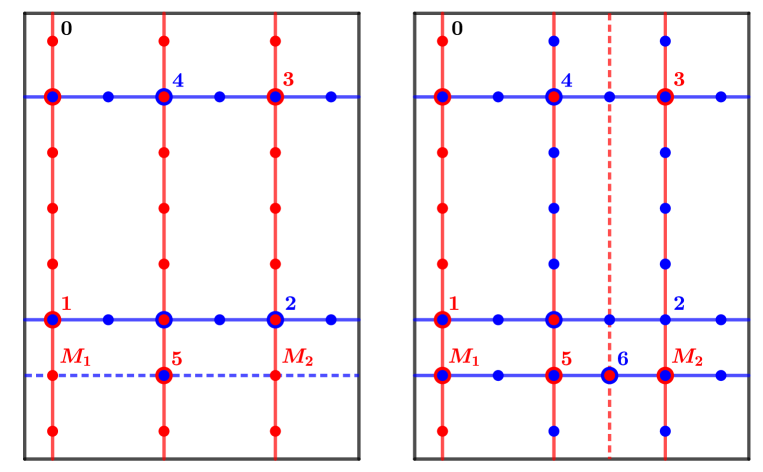
Figure 2: The figure on the left shows an instance of the first five steps of the BRD, whereas the one on the right considers an additional step. Given the position of $\operatorname{\mathsf{BRD}}(t)$ for $t=1,\ldots,5$ in the figure on the left, $D_{n}(5)$ coincides with the event that the payoff of player $\mathrm{B}$ at $5$ is not the maximum of its row (the blue dashed line). Conditioning on $D_{n}(5)$, the probability of $D_{n}(6)$ is the product between the probability that $\operatorname{\mathsf{BRD}}(6)$ is not at the action profiles $M_{1}$ and $M_{2}$, that is $(K_{n}^{\mathrm{B}}-3)/(K_{n}^{\mathrm{B}}-1)$, and, given this, the probability that the payoff of player $\mathrm{A}$ at $6$ is not the maximum of its column (the red dashed line), i.e., $(K_{n}^{\mathrm{A}}-1)/K_{n}^{\mathrm{A}}$. This explains (5.61) when $t=6$. Similarly, conditioning on $D_{n}(5)$, $C_{n}(6)$ is the intersection between two events: the first one is that the position of $\operatorname{\mathsf{BRD}}(6)$ does not coincide with $M_{1}$ and $M_{2}$, which has probability $(K_{n}^{\mathrm{B}}-3)/(K_{n}^{\mathrm{B}}-1)$; the second one is that the payoff of player $\mathrm{A}$ at $6$ is the maximum of its column (the red dashed line), which, conditioning on the first event, has probability $1/K_{n}^{\mathrm{A}}$. This justifies (5.58) when $t=6$.

By explicit computation (see Fig. 2), we get

$$\mathsf{P}\left(C_{n}(t)\mid D_{n}(t-1)\right) =\begin{cases}\frac{1}{K_{n}^{\mathrm{A}}}\frac{K_{n}^{\mathrm{B}}-\left\lfloor\frac{t}{2}\right\rfloor}{K_{n}^{\mathrm{B}}-1}&\text{for $t$ even,}\\ \frac{1}{K_{n}^{\mathrm{B}}}\frac{K_{n}^{\mathrm{A}}-\left\lfloor\frac{t}{2}\right\rfloor}{K_{n}^{\mathrm{A}}-1}&\text{for $t$ odd.}\end{cases}$$ (5.58)

On the other hand, since

$$D_{n}(t)\subseteq D_{n}(t-1),$$ (5.59)

we have

$$\mathsf{P}\left(D_{n}(t)\right)=\mathsf{P}\left(D_{n}(t)\cap D_{n}(t-1)\right)=\mathsf{P}\left(D_{n}(t-1)\right)\mathsf{P}\left(D_{n}(t)\mid D_{n}(t-1)\right).$$ (5.60)

The latter conditional probability can be explicitly computed (see Fig. 2), obtaining

$$\mathsf{P}\left(D_{n}(t)\mid D_{n}(t-1)\right)=\begin{cases}\frac{K_{n}^{\mathrm{A}}-1}{K_{n}^{\mathrm{A}}}\frac{K_{n}^{\mathrm{B}}-\left\lfloor\frac{t}{2}\right\rfloor}{K_{n}^{\mathrm{B}}-1}&\text{for $t$ even,}\\ \frac{K_{n}^{\mathrm{B}}-1}{K_{n}^{\mathrm{B}}}\frac{K_{n}^{\mathrm{A}}-\left\lfloor\frac{t}{2}\right\rfloor}{K_{n}^{\mathrm{A}}-1}&\text{for $t$ odd.}\end{cases}$$ (5.61)

By iterating (5.60) and (5.61), we deduce that, for all $t\leq 2K_{n}-1$ odd,

$$\begin{split}\mathsf{P}\left(D_{n}(t)\right)&=\mathsf{P}\left(D_{n}(t-2)\right)\frac{K_{n}^{\mathrm{A}}-\left\lfloor\frac{t}{2}\right\rfloor}{K_{n}^{\mathrm{A}}}\frac{K_{n}^{\mathrm{B}}-\left\lfloor\frac{t}{2}\right\rfloor}{K_{n}^{\mathrm{B}}}\\ &=\frac{K_{n}^{\mathrm{B}}-1}{K_{n}^{\mathrm{B}}}\prod_{\begin{subarray}{c}j=1\\ j\text{ odd}\end{subarray}}^{\left\lfloor\frac{t}{2}\right\rfloor}\frac{K_{n}^{\mathrm{B}}-j}{K_{n}^{\mathrm{B}}}\frac{K_{n}^{\mathrm{A}}-j}{K_{n}^{\mathrm{A}}}\\ &\leq\prod_{\begin{subarray}{c}j=1\\ j\text{ odd}\end{subarray}}^{\left\lfloor\frac{t}{2}\right\rfloor}\left(1-\frac{j}{K_{n}}\right)\leq\exp\left(-\sum_{\begin{subarray}{c}j=1\\ j\text{ odd}\end{subarray}}^{\left\lfloor\frac{t}{2}\right\rfloor}\frac{j}{K_{n}}\right)\leq\exp\left(-\frac{(t-1)^{2}}{4K_{n}}\right),\end{split}$$ (5.62)

where we have used the inequality $1-x\leq\operatorname{e}^{-x}$.

Moreover, by (5.61), $\mathsf{P}\left(D_{n}(t)\right)$ is decreasing in $t$ and, by (5.58), $\mathsf{P}\left(C_{n}(t)\mid D_{n}(t-1)\right)\leq 1/K_{n}$ for all $t$. Hence, iterating (5.57), we can write

$$\begin{split}\mathsf{P}\left(C_{n}(t)\right)&=\mathsf{P}\left(C_{n}(t-2)\right)+\mathsf{P}\left(C_{n}(t-1)\mid D_{n}(t-2)\right)\mathsf{P}\left(D_{n}(t-2)\right)\\ &\quad+\mathsf{P}\left(C_{n}(t)\mid D_{n}(t-1)\right)\mathsf{P}\left(D_{n}(t-1)\right)\\ &\leq\mathsf{P}\left(C_{n}(t-2)\right)+\frac{2}{K_{n}}\mathsf{P}\left(D_{n}(t-2)\right).\end{split}$$ (5.63)

By applying the estimate in (5.62) to $\mathsf{P}\left(D_{n}(t-2)\right)$, we obtain, for $t$ odd,

$$\mathsf{P}\left(C_{n}(t)\right)\leq\mathsf{P}\left(C_{n}(t-2)\right)+\frac{2}{K_{n}}\exp\left(-\frac{(t-3)^{2}}{4K_{n}}\right),$$ (5.64)

whose iteration leads to

$$\mathsf{P}\left(C_{n}(t)\right)\leq\mathsf{P}\left(C_{n}(1)\right)+\frac{2}{K_{n}}\sum_{\begin{subarray}{c}j=1\\ j\text{ odd}\end{subarray}}^{t-3}\exp\left(-\frac{j^{2}}{4K_{n}}\right)\leq\frac{1}{K_{n}}+\frac{2}{K_{n}}\sum_{\begin{subarray}{c}j=1\\ j\text{ odd}\end{subarray}}^{t-3}\exp\left(-\frac{j^{2}}{4K_{n}}\right)\,,$$ (5.65)

where in the last inequality we have used (5.53).

Taking $t=2K_{n}-1$ and using the estimate $\sum_{j=0}^{H}\exp\left\{-j^{2}/H\right\}=\mathcal{O}(\sqrt{H})$ for $H\to\infty$, we conclude that

$$\mathsf{P}\left(C_{n}(2K_{n}-1)\right)\leq\mathcal{O}\left(\frac{1}{\sqrt{K_{n}}}\right),$$ (5.66)

which implies (4.19). ∎

Proofs of Section 4.4

We now prove the following result, and then show that Proposition 4.7 immediately follows from it.

Proposition 5.2.

Fix a positive sequence $p_{n}$. Then, for every sequence $\ell_{n}$ such that

$$\lim_{n\to\infty}\ell_{n}=\infty,\quad\lim_{n\to\infty}\frac{\log(p_{n})}{\log(\ell_{n})}=0,\quad\text{and}\quad\lim_{n\to\infty}\frac{\ell_{n}}{\sqrt{K_{n}^{\mathrm{A}}\wedge K_{n}^{\mathrm{B}}}}=0,$$ (5.67)

we have

$$\lim_{n\to\infty}\mathsf{P}\left(\tau_{n}^{\operatorname{\mathsf{NE}}}<\ell_{n}\right)=1.$$ (5.68)

The proof of Proposition 5.2 relies on the following lemma.

Lemma 5.3.

Given a sequence $\left\{X_{i}\right\}_{i\in\mathbb{N}_{+}}$ of i.i.d. random variables having a uniform distribution on $[0,1]$, consider the event

$$L=\{X_{1}<\max\{X_{1},\ldots,X_{k}\}\}\,.$$ (5.69)

Then for all $x\in[0,1]$ we have

$$\mathsf{P}(X_{1}\leq x\mid L)\geq x=\mathsf{P}(X_{1}\leq x).$$ (5.70)

Proof.

The conditional distribution of $X_{1}$, given $L^{c}$, is $\operatorname{\mathsf{Beta}}(k,1)$, i.e.,

$$\mathsf{P}(X_{1}\leq x\,|\,L^{c})=x^{k}\leq x\,.$$ (5.71)

Then

$$\begin{split}\mathsf{P}(X_{1}\leq x\mid L)&=\frac{\mathsf{P}(X_{1}\leq x)-\mathsf{P}(X_{1}\leq x\,|\,L^{c})\mathsf{P}(L^{c})}{\mathsf{P}(L)}\\ &=\frac{x-x^{k}\mathsf{P}(L^{c})}{1-\mathsf{P}(L^{c})}\\ &\geq\frac{x-x\mathsf{P}(L^{c})}{1-\mathsf{P}(L^{c})}=x\,,\end{split}$$ (5.72)

where the last inequality is due to (5.71). ∎

Proof of Proposition 5.2.

Define the events

$$E_{n}(t) \coloneqq\left\{\operatorname{\mathsf{BRD}}_{n}(t)\in R_{n}(t-2)\right\},\quad\text{for }t\geq 2,$$ (5.73)

$$Z_{n}(t) \coloneqq\left\{\operatorname{\mathsf{BRD}}_{n}(t)\neq\operatorname{\mathsf{BRD}}_{n}(t-1)\right\},\quad\text{for }t\geq 1,$$ (5.74)

In words, $E_{n}(t)$ represents the event that at time $t$ the process $\operatorname{\mathsf{BRD}}_{n}(t)$ visits a previously visited row or column, that is, $E_{n}(t)=\{\tau_{n}^{R}\leq t\}$, whereas $Z_{n}(t)$ represents the event that $\operatorname{\mathsf{BRD}}_{n}(t-1)$ is not a PNE. Therefore, the sequence $E_{n}(t)$ is increasing in $t$, i.e.,

$$E_{n}(t-1)\subseteq E_{n}(t),$$ (5.75)

whereas the sequence $Z_{n}(t)$ is decreasing in $t$, i.e.,

$$Z_{n}(t-1)\supseteq Z_{n}(t).$$ (5.76)

Then

$$\begin{split}\mathsf{P}\left(E_{n}(t)\cap Z_{n}(t)\right)&=\mathsf{P}\left(E_{n}(t-1)\cap E_{n}(t)\cap Z_{n}(t)\right)+\mathsf{P}\left(E_{n}(t-1)^{c}\cap E_{n}(t)\cap Z_{n}(t)\right)\\ &=\mathsf{P}\left(E_{n}(t-1)\cap Z_{n}(t)\right)+\mathsf{P}\left(E_{n}(t-1)^{c}\cap E_{n}(t)\cap Z_{n}(t)\right)\\ &\leq\mathsf{P}\left(E_{n}(t-1)\cap Z_{n}(t-1)\right)+\mathsf{P}\left(E_{n}(t-1)^{c}\cap E_{n}(t)\cap Z_{n}(t)\right)\\ &\leq\mathsf{P}\left(E_{n}(t-1)\cap Z_{n}(t-1)\right)+\mathsf{P}\left(E_{n}(t)\mid E_{n}(t-1)^{c}\cap Z_{n}(t)\right),\end{split}$$ (5.77)

where the first equality is just the law of total probabilities, the second derives from (5.75), the first inequality is a consequence of (5.76), and the last stems from the definition of conditional probability. Moreover, we claim that, for $t\geq 3$, we have

$$\mathsf{P}\left(E_{n}(t)\mid E_{n}(t-1)^{c}\cap Z_{n}(t)\right)\leq\begin{cases}\frac{\lfloor\frac{t}{2}\rfloor-1}{K_{n}^{\mathrm{B}}-1}&\text{if $t$ is even,}\\ \frac{\lfloor\frac{t}{2}\rfloor-1}{K_{n}^{\mathrm{A}}-1}&\text{if $t$ is odd.}\end{cases}$$ (5.78)

The conditioning event on the l.h.s. of (5.78) represents the fact that $\operatorname{\mathsf{BRD}}_{n}(t-1)$ is neither a PNE nor an element of $R_{n}(t-3)$. Therefore (5.78) provides a bound for the conditional probability that $\operatorname{\mathsf{BRD}}_{n}(t)$ is an element of $R_{n}(t-2)$. To see why the bound holds, start considering the case $p_{n}=0$, where the inequality in (5.78) holds as an equality. This is due to the fact that all payoffs are i.i.d. ​​. On the other extreme, when $p_{n}=1$, the left hand side equals zero, since potential games do not admit traps. In the intermediate case when $p_{n}\in(0,1)$, the payoffs in the row (column) of interest are not i.i.d. ​​. Consider an $\mathrm{A}$ payoff in a previously visited row; with probability $1-p_{n}$ it is uniformly distributed on $[0,1]$ and with probability $p_{n}$ it has the law of a uniform random variable, conditioned on not being the largest payoff in its row. A similar argument holds for $\mathrm{B}$ payoffs, replacing row with column. By Lemma 5.3, the distribution of a $\mathrm{B}$ payoff on a previously visited row ($\mathrm{A}$ payoff on a previously visited column) is stochastically dominated by a uniform distribution on $[0,1]$. This proves the inequality in (5.78).

Iterating (5.77) we obtain

$$\begin{split}\mathsf{P}\left(E_{n}(t)\cap Z_{n}(t)\right)&\leq\mathsf{P}\left(E_{n}(2)\cap Z_{n}(2)\right)+\sum_{i=3}^{t}\frac{\lfloor\frac{i}{2}\rfloor-1}{K_{n}^{\mathrm{A}}\wedge K_{n}^{\mathrm{B}}-1}\\ &\leq\sum_{i=1}^{t}\frac{i}{K_{n}^{\mathrm{A}}\wedge K_{n}^{\mathrm{B}}-1}\leq\frac{t^{2}}{K_{n}^{\mathrm{A}}\wedge K_{n}^{\mathrm{B}}-1},\end{split}$$ (5.79)

where for the last bound we used the fact that $\mathsf{P}\left(E_{n}(2)\cap Z_{n}(2)\right)=0$ (since $\{E_{n}(2)\}=\{Z_{n}(2)^{c}\}$) and the fact $\sum_{i=1}^{t}i=t(t+1)/2$. Call $\tau_{n}^{\operatorname{\mathsf{cycle}}}$ the stopping time

$$\tau_{n}^{\operatorname{\mathsf{cycle}}}\coloneqq\inf\left\{t\geq 4\colon E_{n}(t)\cap Z_{n}(t)\text{ holds}\right\},$$ (5.80)

that is, $\tau_{n}^{\operatorname{\mathsf{cycle}}}$ is the first time that the BRD re-visits an element of a trap. Hence, (5.79) says that for all $p_{n}\in[0,1]$, if $\ell_{n}=o(\sqrt{K_{n}^{\mathrm{A}}\wedge K_{n}^{\mathrm{B}}})$, then, as $n\to\infty$,

$$\mathsf{P}(\tau_{n}^{\operatorname{\mathsf{cycle}}}\leq\ell_{n})\to 0.$$ (5.81)

By definition of $\tau_{n}^{\operatorname{\mathsf{cycle}}}$, the stopping time $\tau_{n}^{R}$ defined in (4.5) can be rewritten as

$$\tau_{n}^{R}\coloneqq\begin{cases}\tau_{n}^{\operatorname{\mathsf{cycle}}}\wedge(\tau_{n}^{\operatorname{\mathsf{NE}}}+1)\,,&\text{if }(1,1)\not\in\operatorname{\mathsf{NE}}_{n}\,,\\ 2\,,&\text{if }(1,1)\in\operatorname{\mathsf{NE}}_{n}\,.\end{cases}$$ (5.82)

Notice that, for every sequence $\ell_{n}=o\left(\sqrt{K_{n}^{\mathrm{A}}\wedge K_{n}^{\mathrm{B}}}\right)$, if we show that

$$\mathsf{P}\left(\tau_{n}^{R}\leq\ell_{n}\right)\to 1,$$ (5.83)

then from (5.81) and (5.82) it follows that

$$\mathsf{P}\left(\tau_{n}^{\operatorname{\mathsf{NE}}}\leq\ell_{n}\right)\to 1.$$ (5.84)

Let

$$S_{n}\coloneqq\left\{(a,b)\in[K_{n}^{\mathrm{A}}]\times[K_{n}^{\mathrm{B}}]\colon U^{\mathrm{A}}_{n}(a,b)=U^{\mathrm{B}}_{n}(a,b)\right\},$$ (5.85)

be the set of action profiles that give the same payoff to the two players. Fix now a sequence $\ell_{n}=o\left(\sqrt{K_{n}^{\mathrm{A}}\wedge K_{n}^{\mathrm{B}}}\right)$ and define, for every integer $s\in\left\{1,\dots,\ell_{n}-1\right\}$,

$$J_{n}^{s,\ell_{n}}\coloneqq\left\{\exists t\leq\ell_{n}-s\ \text{ s.t. }\operatorname{\mathsf{BRD}}_{n}(t+s^{\prime})\in S_{n},\quad\forall s^{\prime}\in\{0,\dots,s\}\right\}.$$ (5.86)

The event $J_{n}^{s,\ell_{n}}$ occurs if there exists an interval of $s$ consecutive steps before $\ell_{n}$ in which the BRD visits only elements in $S_{n}$.

For every sequence $(s_{n})_{n\in\mathbb{N}}$ such that $s_{n}\leq\ell_{n}$ for every $n$, we have

$$\mathsf{P}(\tau_{n}^{R}>\ell_{n})=\mathsf{P}\left(\left\{\tau_{n}^{R}>\ell_{n}\right\}\cap J_{n}^{s_{n},\ell_{n}}\right)+\mathsf{P}\left(\left\{\tau_{n}^{R}>\ell_{n}\right\}\cap\left\{J_{n}^{s_{n},\ell_{n}}\right\}^{c}\right).$$ (5.87)

First we show that the first term on the r.h.s. of (5.87) goes to zero as $s_{n}\to\infty$. To this end, it is enough to show that, under the event $J_{n}^{s_{n},\ell_{n}}$, there exists some $t\leq\ell_{n}-s_{n}$ such that the best-responding player’s payoff at time $t+s_{n}$ is stochastically larger than a $\operatorname{\mathsf{Beta}}(u,1)$ random variable, with

$$u\coloneqq r_{n}(s_{n})-\frac{\ell_{n}^{2}}{4}.$$ (5.88)

Notice that, for $n\in\mathbb{N}$ large enough,

$$u\geq\frac{s_{n}}{2}(K_{n}^{\mathrm{A}}+K_{n}^{\mathrm{B}})-\frac{\ell_{n}^{2}}{2}\geq\frac{s_{n}}{3}(K_{n}^{\mathrm{A}}+K_{n}^{\mathrm{B}}),$$ (5.89)

where in the first inequality we used (4.8) and the fact that $s_{n}\leq\ell_{n}$; the second inequality holds for all sufficiently large $n$ by our choice of $\ell_{n}$. Indeed, after the interval of $s_{n}$ consecutive steps in which the BRD visits only elements of $S_{n}$, the BRD visits an action profile $(a,b)$ such that

• $(a,b)\in S_{n}$, that is, both players receive the same payoff;

• this common payoff is the largest of a set of random variables, among which at least $u$ are i.i.d. $\operatorname{\mathsf{Unif}}([0,1])$ (see Fig. 3 for more details);

hence, the stochastic domination follows.

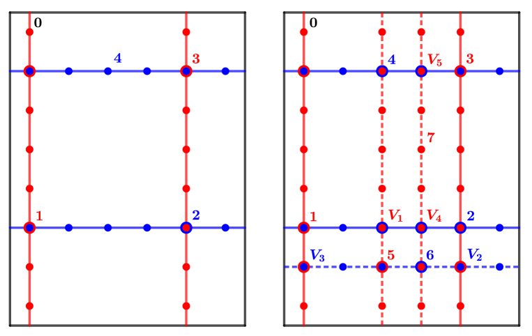
Figure 3: The left figure shows an instance of the first four steps of the BRD. The right figure shows how the dynamics proceeds after time $4$. The numbered action profiles lying on the dashed lines, i.e., $5$, $6$, and $7$, give the same payoff to the row and column player. Note that in this case the event $J_{n}^{s_{n},\ell_{n}}$ occurs with $\ell_{n}=7$ and $s_{n}=3$. Indeed, there exists $t\leq\ell_{n}-s_{n}$ (in this case $t=4$) such that the BRD visits only action profiles in $S_{n}$ for $s_{n}$ consecutive steps. As a consequence, the payoff of the row player at the action profile $7$ is the maximum of the payoffs of the row player in the action profiles lying on the red dashed lines and of the payoffs of the column player in the action profiles lying on the blue dashed lines. Such payoffs are all i.i.d. $\operatorname{\mathsf{Unif}}([0,1])$ except for the payoffs associated to the action profiles $4,V_{1},\ldots,V_{5}$, for which we have additional information. Since the number of such exceptional action profiles is at most $\left(\ell_{n}/2\right)^{2}$ and the total number of action profiles lying on the dashed lines is $r_{n}(s_{n})$, we have that the payoff of the row player at the action profile $7$ is the maximum of at least $u$ i.i.d. $\operatorname{\mathsf{Unif}}([0,1])$ random variables, where $u$ is defined as in (5.88).

Therefore, by Proposition B.1, the probability that $\operatorname{\mathsf{BRD}}_{n}(t+s_{n})=\operatorname{\mathsf{BRD}}_{n}(t+s_{n}+1)$, that is, $\operatorname{\mathsf{BRD}}_{n}(t+s_{n})$ is a PNE, is bounded from below by the probability that a $\operatorname{\mathsf{Beta}}(u,1)$ random variable is larger than the maximum of $K_{n}^{\mathrm{A}}\vee K_{n}^{\mathrm{B}}-1$ i.i.d. random variables with a uniform distribution on $[0,1]$. Hence, by Proposition B.2, we get

$$\mathsf{P}\left(\left\{\tau_{n}^{R}>\ell_{n}\right\}\cap J_{n}^{s_{n},\ell_{n}}\right)\leq 1-\frac{\left\lfloor\frac{s_{n}}{3}\right\rfloor(K_{n}^{\mathrm{A}}+K_{n}^{\mathrm{B}})}{\left\lfloor\frac{s_{n}}{3}\right\rfloor(K_{n}^{\mathrm{A}}+K_{n}^{\mathrm{B}})+(K_{n}^{\mathrm{A}}\vee K_{n}^{\mathrm{B}}-1)}\leq\frac{3}{s_{n}+3},$$ (5.90)

which goes to zero as $s_{n}\to\infty$. We now show that, under the assumption in (5.67), it is possible to find a sequence $(s_{n})_{n}$ such that

$$\lim_{n\to\infty}s_{n}=\infty,\qquad\lim_{n\to\infty}\frac{s_{n}}{\ell_{n}}=0,$$ (5.91)

and

$$\lim_{n\to\infty}\mathsf{P}\left(\left\{\tau_{n}^{R}>\ell_{n}\right\}\cap\left\{J_{n}^{s_{n},\ell_{n}}\right\}^{c}\right)\to 0.$$ (5.92)

Notice that under the event $\left\{\tau_{n}^{R}>\ell_{n}\right\}$, the probability of the event $\left\{J_{n}^{s_{n},\ell_{n}}\right\}^{c}$ can be upper bounded by the probability that, splitting the interval $\left\{0,\dots,\ell_{n}\right\}$ into subintervals of length $s_{n}$, none of them is such that the BRD visits only $S_{n}$ in that subinterval. Therefore,

$$\mathsf{P}\left(\left\{\tau_{n}^{R}>\ell_{n}\right\}\cap\left\{J_{n}^{s_{n},\ell_{n}}\right\}^{c}\right)\leq\mathsf{P}\left(\operatorname{\mathsf{Binomial}}\left(\left\lfloor\frac{\ell_{n}}{s_{n}}\right\rfloor,p_{n}^{s_{n}}\right)=0\right)=(1-p_{n}^{s_{n}})^{\left\lfloor\ell_{n}/s_{n}\right\rfloor}.$$ (5.93)

If $\ell_{n}=o(\sqrt{K_{n}^{\mathrm{A}}\wedge K_{n}^{\mathrm{B}}})$, then the term on the r.h.s. of (5.93) goes to zero whenever

$$\lim_{n\to\infty}\frac{\ell_{n}}{s_{n}}p_{n}^{s_{n}}=\infty.$$ (5.94)

A necessary and sufficient condition for (5.94) is

$$\lim_{n\to\infty}\log(\ell_{n})-\log(s_{n})-s_{n}\log(p_{n}^{-1})=\infty,$$ (5.95)

or, equivalently,

$$\lim_{n\to\infty}\log(\ell_{n})\left[1-\frac{\log(s_{n})}{\log(\ell_{n})}-\frac{s_{n}\log(p_{n}^{-1})}{\log(\ell_{n})}\right]=\infty.$$ (5.96)

Thanks to (5.67), we can choose, e.g.,

$$s_{n}=\log(\ell_{n})\wedge\log\left(\frac{\log(\ell_{n})}{\log(p_{n}^{-1})}\right)\to\infty.$$ (5.97)

Since, for every diverging positive sequence $(a_{n})_{n\geq 0}$, it holds that $\log(a_{n})/a_{n}\to 0$, by the definition in (5.97) we deduce that

$$\frac{\log(s_{n})}{\log(\ell_{n})}\leq\frac{\log(\log\ell_{n})}{\log(\ell_{n})}\to 0\quad\text{as}\quad n\to\infty\,,$$ (5.98)

and

$$\frac{s_{n}\log(p_{n}^{-1})}{\log(\ell_{n})}\leq\frac{\log\left(\dfrac{\log(\ell_{n})}{\log(p_{n}^{-1})}\right)}{\dfrac{\log(\ell_{n})}{\log(p_{n}^{-1})}}\to 0\quad\text{as}\quad n\to\infty\,.$$ (5.99)

Coupling (5.98) and (5.99), we immediately validate (5.96). ∎

Proof of Proposition 4.7.

Assume that (4.20) is satisfied. Choose any sequence $\ell_{n}$ such that

$$\lim_{n\to\infty}\frac{\log(p_{n})}{\log(\ell_{n})}=0.$$ (5.100)

There are two cases:

• If

  $$\lim_{n\to\infty}\frac{\ell_{n}}{\sqrt{K_{n}^{\mathrm{A}}\wedge K_{n}^{\mathrm{B}}}}=0,$$

  then (4.23) follows by Proposition 5.2.

• If instead

  $$\limsup_{n\to\infty}\frac{\ell_{n}}{\sqrt{K_{n}^{\mathrm{A}}\wedge K_{n}^{\mathrm{B}}}}>0,$$ (5.101)

  then we can define the $\ell_{n}^{\prime}=\ell_{n}\wedge\lceil K_{n}^{\mathrm{A}}\wedge K_{n}^{\mathrm{B}}\rceil^{1/3}$. Notice that

  • $\lim_{n\to\infty}\ell_{n}^{\prime}=\infty$;

  • by the fact that $\log(\ell_{n}^{\prime})\geq\frac{1}{3}\log(K_{n}^{\mathrm{A}}\wedge K_{n}^{\mathrm{B}})\wedge\log(\ell_{n})$, combined with (4.20) and (5.100), we deduce that

    $$\lim_{n\to\infty}\frac{\log(p_{n})}{\log(\ell_{n}^{\prime})}=0;$$

  • moreover, by the definition of $\ell_{n}^{\prime}$ we have

    $$\lim_{n\to\infty}\frac{\ell_{n}^{\prime}}{\sqrt{K_{n}^{\mathrm{A}}\wedge K_{n}^{\mathrm{B}}}}=0.$$

  Hence, thanks to Proposition 5.2 we get

  $$\lim_{n\to\infty}\mathsf{P}\left(\tau_{n}^{\operatorname{\mathsf{NE}}}<\ell_{n}^{\prime}\right)=1.$$ (5.102)

  To conclude the proof, it is enough to see that for every $n\in\mathbb{N}$

  $$\mathsf{P}\left(\tau_{n}^{\operatorname{\mathsf{NE}}}<\ell_{n}\right)\geq\mathsf{P}\left(\tau_{n}^{\operatorname{\mathsf{NE}}}<\ell_{n}^{\prime}\right).\qed$$

6 Conclusions and open problems

We have considered a model of two-person games with random payoffs that parametrically interpolates potential games and games with i.i.d. payoffs. The interpolation acts locally on each payoff profile. We have studied both the asymptotic behavior of the random number of pure Nash equilibria of the game and the asymptotic behavior of best response dynamics, as the number of actions for each player diverges. The type of model that we chose requires combinatorial tools for its analysis.

We see this paper as a first attempt to provide a parametric model for random games where the payoffs are not independent, but have some structure that depends on a locally acting parameter. Several extensions and variations of this model are conceivable and will be the object of our future research. For instance:

1. It would be interesting to have a clearer view of the phase transition taking place at $p=0$. In particular, it would be important to investigate the existence of a sequence $p_{n}\to 0$ such that the probability that a BRD does not lead to a PNE converges to a value smaller than $1$.

2. Games with more than two players could be studied.

3. With more than two players, different types of deviator rules in BRD could be considered, e.g., round-robin, random order, etc..

4. The behavior of better-response dynamics could be studied and compared to best response dynamics, along the lines of Amiet et al., 2021a .

5. When we deal with the number of pure Nash equilibria, we studied a form of Law of Large Numbers. The existence of a Central Limit Theorem could be explored.

Appendix A List of symbols

$A_{a}$	$\left\{\text{player $\mathrm{A}$'s best response to action $1$ is $a$}\right\}$, defined in (5.16)
$\operatorname{\mathsf{BRD}}$	best response dynamics
$C_{n}(t)$	$\left\{\operatorname{\mathsf{BRD}}_{n}(t)\in\operatorname{\mathsf{NE}}_{n}\right\}$, defined in (5.49)
$D_{n}(t)$	$\left\{\operatorname{\mathsf{BRD}}_{n}(t)\not\in\operatorname{\mathsf{NE}}_{n},\ \operatorname{\mathsf{BRD}}_{n}(t)\not\in R_{n}(t-2)\right\}$, defined in (5.49)
$E_{n}(t)$	$\left\{\operatorname{\mathsf{BRD}}(t)\in R_{n}(t-2)\right\}$, defined in (5.73)
$F$	uniform distribution function on $[0,1]$
$G_{t}^{\pi}$	$\left\{\operatorname{\mathsf{BRD}}_{n}(s)=\pi_{s}\text{ for }0\leq s\leq t\right\}$, defined in (5.19)
$H_{n}$	distribution function of $\tau_{n}^{\operatorname{\mathsf{NE}}}$
$J_{n}^{s,\ell_{n}}$	$\left\{\exists t\leq\ell_{n}-s\ \text{ s.t. }\operatorname{\mathsf{BRD}}_{n}(t+s^{\prime})\in S_{n},\forall s^{\prime}\in\{0,\dots,s\}\right\}$, defined in (5.86)
$K_{n}^{\mathrm{A}}$	number of player $\mathrm{A}$’s actions in the game $\boldsymbol{U}_{n}$
$K_{n}^{\mathrm{B}}$	number of player $\mathrm{B}$’s actions in the game $\boldsymbol{U}_{n}$
$K_{n}$	$\min(K_{n}^{\mathrm{A}},K_{n}^{\mathrm{B}})$, defined in (3.2)
$[K^{\mathrm{A}}]$	action set of player $\mathrm{A}$
$[K^{\mathrm{B}}]$	action set of player $\mathrm{B}$
$L$	$\{X_{1}<\max\{X_{1},\ldots,X_{k}\}\}$, defined in (5.69)
$M$	trap, defined in Definition 2.1
$\operatorname{\mathsf{NE}}$	set of pure Nash equilibria
$p_{n}$	probability that $U^{\mathrm{A}}(a,b)=U^{\mathrm{B}}(a,b)$ in the game $\boldsymbol{U}_{n}$
$q_{t,n}$	$\mathsf{P}\left(\tau_{n}^{\operatorname{\mathsf{NE}}}=t\mid\tau_{n}^{\operatorname{\mathsf{NE}}}\geq t\right)$, defined in (4.12)
$r_{n}(t)$	$\left\lceil\dfrac{t+1}{2}\right\rceil K_{n}^{\mathrm{A}}+\left\lfloor\dfrac{t+1}{2}\right\rfloor K_{n}^{\mathrm{B}}-\left\lfloor\dfrac{t+1}{2}\right\rfloor\left\lceil\dfrac{t+1}{2}\right\rceil$, defined in (4.8)
$R_{n}(t)$	defined in (4.3)
$S_{n}$	$\left\{(a,b)\in[K_{n}^{\mathrm{A}}]\times[K_{n}^{\mathrm{B}}]\colon U^{\mathrm{A}}_{n}(a,b)=U^{\mathrm{B}}_{n}(a,b)\right\}$, defined in (5.85)
$t$	(discrete) time
$U^{\mathrm{A}}$	player $\mathrm{A}$’s payoff function
$U^{\mathrm{B}}$	player $\mathrm{B}$’s payoff function
$W_{n}$	number of pure Nash equilibria in $\boldsymbol{U}_{n}$
$Z_{n}(t)$	$\left\{\operatorname{\mathsf{BRD}}_{n}(t)\neq\operatorname{\mathsf{BRD}}_{n}(t-1)\right\}$, defined in (5.74)
$\Pi_{t}$	set of possible paths for $\operatorname{\mathsf{BRD}}_{n}$ up to time $t$
$\tau_{n}^{\operatorname{\mathsf{NE}}}$	first time the BRD visits a PNE, defined in (4.2)
$\tau_{n}^{\operatorname{\mathsf{cycle}}}$	first time the BRD re-visits an element of a trap, defined in (5.80)
$\tau^{R}_{n}$	$\min\left\{t\geq 2:\ \operatorname{\mathsf{BRD}}_{n}(t)\in R_{n}(t-2)\right\}$, defined in (4.5)
$\Phi_{n}(t)$	$\int_{0}^{t}H_{n}(s)\ \textup{d}s$, defined in (5.39)
$\Psi$	potential function, defined in (2.4)

Appendix B Beta distribution

We report two well-known results about Beta distributions. For the sake of completeness, we add their simple proofs.

Proposition B.1.

Let $X_{1},\ldots,X_{k}$ be i.i.d. random variables having a uniform distribution on $[0,1]$ and let $M_{k}\coloneqq\max_{i\in\{1,\dots,k\}}X_{i}$. Then $M_{k}$ has distribution $\operatorname{\mathsf{Beta}}(k,1)$.

Proof.

For any $t\in[0,1]$ we have

$$\mathsf{P}(M_{k}\leq t)=[\mathsf{P}(X_{1}\leq t)]^{k}=t^{k},$$

i.e., a $\operatorname{\mathsf{Beta}}(k,1)$ distribution function. ∎

Proposition B.2.

Let $X$ and $Y$ be independent random variables with distributions $\operatorname{\mathsf{Beta}}(a,1)$ and $\operatorname{\mathsf{Beta}}(b,1)$, respectively. Then

$$\mathsf{P}(X>Y)=\frac{a}{a+b}\,.$$ (B.1)

Proof.

We have

$$\mathsf{P}(X>Y) =\int_{0}^{1}\left(\int_{0}^{t}at^{a-1}\cdot bs^{b-1}\ \textup{d}s\right)\ \textup{d}t=\int_{0}^{1}at^{a-1}\cdot t^{b}\ \textup{d}t=\frac{a}{a+b}\,.\qed$$

References

• Alon et al., (2021) Alon, N., Rudov, K., and Yariv, L. (2021). Dominance solvability in random games. Technical report, arXiv 2105.10743.
• (2) Amiet, B., Collevecchio, A., and Hamza, K. (2021a). When “better” is better than “best”. Oper. Res. Lett., 49(2):260–264.
• (3) Amiet, B., Collevecchio, A., Scarsini, M., and Zhong, Z. (2021b). Pure Nash equilibria and best-response dynamics in random games. Math. Oper. Res., 46(4):1552–1572.
• Baldi et al., (1989) Baldi, P., Rinott, Y., and Stein, C. (1989). A normal approximation for the number of local maxima of a random function on a graph. In Probability, Statistics, and Mathematics, pages 59–81. Academic Press, Inc.
• Candogan et al., (2011) Candogan, O., Menache, I., Ozdaglar, A., and Parrilo, P. A. (2011). Flows and decompositions of games: harmonic and potential games. Math. Oper. Res., 36(3):474–503.
• Candogan et al., (2013) Candogan, O., Ozdaglar, A., and Parrilo, P. A. (2013). Dynamics in near-potential games. Games Econom. Behav., 82:66–90.
• Coucheney et al., (2014) Coucheney, P., Durand, S., Gaujal, B., and Touati, C. (2014). General revision protocols in best response algorithms for potential games. In Netwok Games, Control and OPtimization (NetGCoop), Trento, Italy. IEEE Explore.
• Durand et al., (2019) Durand, S., Garin, F., and Gaujal, B. (2019). Distributed best response dynamics with high playing rates in potential games. Performance Evaluation, 129:40–59.
• Durand and Gaujal, (2016) Durand, S. and Gaujal, B. (2016). Complexity and optimality of the best response algorithm in random potential games. In Algorithmic Game Theory, volume 9928 of Lecture Notes in Comput. Sci., pages 40–51. Springer, Berlin.
• Fabrikant et al., (2013) Fabrikant, A., Jaggard, A. D., and Schapira, M. (2013). On the structure of weakly acyclic games. Theory Comput. Syst., 53(1):107–122.
• Galla and Farmer, (2013) Galla, T. and Farmer, J. D. (2013). Complex dynamics in learning complicated games. Proc. Natl. Acad. Sci. USA, 110(4):1232–1236.
• Goemans et al., (2005) Goemans, M., Mirrokni, V., and Vetta, A. (2005). Sink equilibria and convergence. In 46th Annual IEEE Symposium on Foundations of Computer Science (FOCS’05), pages 142–151.
• Harsanyi, (1973) Harsanyi, J. C. (1973). Oddness of the number of equilibrium points: a new proof. Internat. J. Game Theory, 2:235–250.
• Heinrich et al., (2023) Heinrich, T., Jang, Y., Mungo, L., Pangallo, M., Scott, A., Tarbush, B., and Wiese, S. (2023). Best-response dynamics, playing sequences, and convergence to equilibrium in random games. Internat. J. Game Theory, 52(3):703–735.
• Johnston et al., (2023) Johnston, T., Savery, M., Scott, A., and Tarbush, B. (2023). Game connectivity and adaptive dynamics. Technical report, arXiv 2309.10609.
• Karlin and Peres, (2017) Karlin, A. R. and Peres, Y. (2017). Game Theory, Alive. American Mathematical Society, Providence, RI.
• Monderer and Shapley, (1996) Monderer, D. and Shapley, L. S. (1996). Potential games. Games Econom. Behav., 14(1):124–143.
• Nash, (1951) Nash, J. (1951). Non-cooperative games. Ann. of Math. (2), 54:286–295.
• Nash, (1950) Nash, Jr., J. F. (1950). Equilibrium points in $n$-person games. Proc. Nat. Acad. Sci. U.S.A., 36:48–49.
• Ogryczak and Ruszczyński, (1999) Ogryczak, W. and Ruszczyński, A. (1999). From stochastic dominance to mean-risk models: Semideviations as risk measures. European J. Oper. Res., 116(1):33–50.
• Pangallo et al., (2019) Pangallo, M., Heinrich, T., and Farmer, J. D. (2019). Best reply structure and equilibrium convergence in generic games. Science Advances, 5(2):eaat1328.
• Pei and Takahashi, (2019) Pei, T. and Takahashi, S. (2019). Rationalizable strategies in random games. Games Econom. Behav., 118:110–125.
• Powers, (1990) Powers, I. Y. (1990). Limiting distributions of the number of pure strategy Nash equilibria in $N$-person games. Internat. J. Game Theory, 19(3):277–286.
• Rinott and Scarsini, (2000) Rinott, Y. and Scarsini, M. (2000). On the number of pure strategy Nash equilibria in random games. Games Econom. Behav., 33(2):274–293.
• Rosenthal, (1973) Rosenthal, R. W. (1973). A class of games possessing pure-strategy Nash equilibria. Internat. J. Game Theory, 2:65–67.
• Sanders et al., (2018) Sanders, J. B. T., Farmer, J. D., and Galla, T. (2018). The prevalence of chaotic dynamics in games with many players. Scientific Reports, 8(1):4902.
• Stanford, (1995) Stanford, W. (1995). A note on the probability of $k$ pure Nash equilibria in matrix games. Games Econom. Behav., 9(2):238–246.
• Wiese and Heinrich, (2022) Wiese, S. C. and Heinrich, T. (2022). The frequency of convergent games under best-response dynamics. Dyn. Games Appl., 12(2):689–700.
• Wilson, (1971) Wilson, R. (1971). Computing equilibria of $N$-person games. SIAM J. Appl. Math., 21:80–87.