Learning Provably Stable Local Volt/Var Controllers for Efficient Network Operation

Abstract

This paper develops a data-driven framework to synthesize local Volt/Var control strategies for distributed energy resources (DERs) in power distribution networks (DNs). Aiming to improve DN operational efficiency, as quantified by a generic optimal reactive power flow (ORPF) problem, we propose a two-stage approach. The first stage involves learning the manifold of optimal operating points determined by an ORPF instance. To synthesize local Volt/Var controllers, the learning task is partitioned into learning local surrogates (one per DER) of the optimal manifold with voltage input and reactive power output. Since these surrogates characterize efficient DN operating points, in the second stage, we develop local control schemes that steer the DN to these operating points. We identify the conditions on the surrogates and control parameters to ensure that the locally acting controllers collectively converge, in a global asymptotic sense, to a DN operating point agreeing with the local surrogates. We use neural networks to model the surrogates and enforce the identified conditions in the training phase. AC power flow simulations on the IEEE 37-bus network empirically bolster the theoretical stability guarantees obtained under linearized power flow assumptions. The tests further highlight the optimality improvement compared to prevalent benchmark methods.

I Introduction

The deployment of a massive number of distributed energy resources (DERs) in power distribution networks (DNs) is dramatically changing the electric power grid. Primarily driven by sustainability and economic incentives, DERs present additional opportunities including reduction of the power generation cost and of greenhouse gas emissions. Nevertheless, DERs’ uncoordinated power injections or sudden generation changes could pose challenges to system operations and stability, e.g., induce undesirable voltage deviations in distribution grids. To facilitate their integration in power grids, DERs are being provided with sensing and computation capabilities, hence becoming smart agents. DERs can exploit the flexibility of their power electronic interface to perform, among other ancillary services, reactive power control. They can also take advantage of the widespread availability of data from DNs and the increased capabilities for storing and processing it to learn effective control policies. This paper aims to leverage learning in the synthesis of local Volt/Var controllers for voltage regulation incorporating optimality considerations and rigorous performance guarantees.

Literature Review

The goal of Volt/Var control strategies is to keep voltages within safe preassigned limits. Even though pertinent standards allow DERs to provide reactive power compensations following static Volt/VAR control rules, see, the IEEE Std. 1547 [1], the literature has provided a variety of options for voltage regulation. Given the massive number of DERs envisioned to be hosted in future DNs, decentralized approaches are often advocated for practical applications. Among decentralized solutions, we have the notable class of distributed algorithms, in which agents can communicate and share information with some peers (e.g., their neighbors), and local algorithms, in which each agent makes decision based only on information available locally. Several distributed schemes have been proposed to solve various instances of optimal power flow (OPF) problems, see e.g. [2]. Optimization-based feedback controllers that steer the network towards equilibrium points that are solutions to OPF problems based on the cyclical alternation of sensing, communication, and actuation have become recently popular [3, 4, 5, 6]. Nevertheless, distributed strategies usually have precise and strict requirements on the communication network. For instance, in many works, each generator is required to share information with all its neighbors in the power network. In local schemes, reactive power compensations are adjusted based merely on measurements taken at the point of connection of the power inverter to the grid [3, 7, 8, 9]. Though much simpler than distributed strategies, local schemes in general do not bring the network towards optimal configurations and have intrinsic performance limitations, e.g., they might fail to regulate voltages even if the overall generation resources are enough [10].

Recent advances in data-driven and learning-based control seek to leverage data from DNs to enhance the performance of local control schemes and reduce its gap with distributed and/or optimal controllers. Reinforcement learning (RL) has emerged as an attractive method to learn optimal control policies from data obtained by interacting with the environment [11]. The works most closely related to this paper include [12] and [13], where RL is used to learn stability-guaranteed local Volt/Var control schemes. However, the former enforces too stringent derivative constraints on the policies to be searched, while the latter only guarantees the voltages converge to a region, instead of an equilibrium point, and both of them require the control policy to be continuously differentiable. Furthermore, neither of them takes into account the reactive power capacity limitations, which are critical when dealing with small-size generators. Another appealing method is to learn deep neural network (DNN)-based predictor of OPF minimizers. A dataset for learning predictors can be created by solving OPF problems using historical consumption and generation data, e.g., smart meter data. Then, DNN-based surrogates are trained to predict the solutions of OPF problems. This has resulted in fruitful results, e.g., [14, 15, 16], to mention a few. In particular, [17, 18] train DNNs to fit not only OPF minimizers, but also their sensitivities with respect to the problem inputs, which significantly improve the prediction accuracy. However, these works still require information across the network as the inputs of the DNNs. Recent works [19, 20] leverage segmented linear regression techniques to learn local surrogates that predict OPF solutions. Though only local measurements are needed to perform the prediction, there is no provable stability guarantees.

Statement of Contributions

We propose a data-driven framework for synthesizing local Volt/Var controllers aiming to improve DN operation efficiency. We formulate a generic optimal reactive power flow (ORPF) problem whose solutions describe optimal network configurations. Our idea starts from using the solutions to the ORPF problem as experts to learn functions of voltages acting as surrogates (one per DER) that characterize efficient operating points of DN. We propose a local control scheme that steers the DN to efficient operating points defined by the surrogates, and identify conditions on the surrogates and control parameters that ensure the algorithm convergence. Compared to the recent literature[3, 7, 8], our synthesis of the local control scheme is neither forced to be linear nor to satisfy stringent slope limitations. This leads to an enlarged search space of potential candidates of desired surrogates. Building on the above idea, we construct a labeled dataset of ORPF solutions with different power profiles and parameterize the surrogates using single hidden layer neural networks, which satisfy the identified conditions by design. We train the neural networks to find the surrogates that minimize the prediction error compared to ORPF solutions. AC power flow simulations on the IEEE 37-bus power system using the proposed data-driven local Volt/Var control design validate the guaranteed stability and significantly improved optimality with respect to prevalent benchmark methods. This work differs from its preliminary version [21] mainly in: relaxing the differentiability requirement on the control rule, allowing it to be just Lipschitz; establishing global, rather than local, stability guarantee for the control scheme; providing a more general design of neural networks in the learning process; and introducing the concept of fictional data points to enhance the voltage regulation capability of learned controllers when voltages are not within desired limits.

Notation

Throughout the paper, $\mathbb{R}$ and $\mathbb{C}$ denote the set of real and complex numbers, respectively. Upper and lower case boldface letters denote matrices and column vectors, respectively. Sets are represented by calligraphic symbols. Given a vector $\mathbf{a}$ (a diagonal matrix $\mathbf{A}$), its $n$-th (diagonal) entry is denoted by $a_{n}$ $(A_{n})$. $\mathbf{A}\succ(\succeq)0$ denotes that matrix $\mathbf{A}$ is positive (semi-) definite, and $\mathbf{A}\prec(\preceq)0$ denotes that matrix $\mathbf{A}$ is negative (semi-) definite. The symbol $(\cdot)^{\top}$ stands for transposition, and $\mathbf{1},\mathbf{0},\mathbf{I}$ denote vectors of all ones and zeros and identity matrix with appropriate dimensions, respectively. Operators $\Re(\cdot)$ and $\Im(\cdot)$ extract the real and imaginary parts of a complex-valued argument, and act element-wise. With a slight abuse of notation, we use $|\cdot|$ to denote the absolute value for real-valued arguments, the magnitude for complex-valued arguments, and the cardinality when the argument is a set. $\|\cdot\|$ represents the Euclidean norm. Given a symmetric matrix $\mathbf{A}$, $\lambda_{\max}(\mathbf{A})$ and $\lambda_{\min}(\mathbf{A})$ represent its largest and smallest eigenvalue, respectively. For any matrix $\mathbf{B}$, it holds that $\|\mathbf{B}\|=\sqrt{\lambda_{\max}(\mathbf{B}^{\top}\mathbf{B})}$. The graph of a function $\phi:\mathbb{R}\rightarrow\mathbb{R}$ is the set of all points of the form $(x,\phi(x))$, whereas the range of $\phi$ is the set of its possible output values.

II Power distribution grid model

Consider a power distribution network with $N+1$ buses modeled by an undirected graph $\mathcal{G}=(\mathcal{N},\mathcal{E})$, where $\mathcal{N}=\{0,1,\dots,N\}$ are associated with the electrical buses and $\mathcal{E}$ represents the set of the electrical lines between these buses. We label the substation node as 0, and assume that it behaves as an ideal voltage source imposing the nominal voltage of 1 p.u. Define the following quantities:

• $u_{n}\in\mathbb{C}$ is the voltage phasor at bus $n\in\mathcal{N}$;

• $v_{n}\in\mathbb{R}$ is the voltage magnitude at bus $n\in\mathcal{N}$;

• $i_{n}\in\mathbb{C}$ is the injected current phasor at bus $n\in\mathcal{N}$;

• $s_{n}=p_{n}+iq_{n}\in\mathbb{C}$ is the nodal complex power injection at bus $n\in\mathcal{N}$, where $p_{n},q_{n}\in\mathbb{R}$ are the active and reactive powers, respectively. Powers take positive (negative) values, i.e., $p_{n},q_{n}\geq 0$ ($p_{n},q_{n}\leq 0$), when they are injected into (absorbed from) the grid.

We use vectors $\mathbf{u},\mathbf{i},\mathbf{s}\in\mathbb{C}^{N}$ to collect the complex voltages, currents, and complex powers of buses $1,2,\ldots,N$, and vectors $\mathbf{v},\mathbf{p},\mathbf{q}\in\mathbb{R}^{N}$ to collect their voltage magnitudes, active and reactive power injections. Denote by $z_{e}\in\mathbb{C}$ and by $y_{e}=z_{e}^{-1}\in\mathbb{C}$ respectively the impedance and the admittance of line $e=(m,n)\in\mathcal{E}$. The network bus admittance matrix $\mathbf{Y}\in\mathbb{C}^{(N+1)\times(N+1)}$ is a symmetric matrix that can be expressed as $\mathbf{Y}=\mathbf{Y}_{L}+{\rm diag}(\mathbf{y}_{T})$, where

$$(\mathbf{Y}_{L})_{mn}=\begin{cases}-y_{(m,n)}&\text{ if }(m,n)\in\mathcal{E},m\neq n,\\ 0&\text{ if }(m,n)\notin\mathcal{E},m\neq n,\\ \sum_{k\neq n}y_{(k,n)}&\text{ if }m=n,\end{cases}$$

and the vector $\mathbf{y}_{T}$ collects the shunt components of each bus. The matrix $\mathbf{Y}_{L}$ is a complex Laplacian matrix, and hence satisfies $\mathbf{Y}_{L}\mathbf{1}=\mathbf{0}$. We partition the bus admittance matrix by separating the components associated with the substation and the ones associated with the other nodes, obtaining

$$\mathbf{Y}=\begin{bmatrix}y_{0}&\mathbf{y}_{0}^{\top}\\ \mathbf{y}_{0}&\tilde{\mathbf{Y}}\end{bmatrix},$$

with $y_{0}\in\mathbb{C}$, $\mathbf{y}_{0}\in\mathbb{C}^{N}$, and $\tilde{\mathbf{Y}}\in\mathbb{C}^{N\times N}$. If the network is connected, then $\tilde{\mathbf{Y}}$ is invertible [22]. Let $\tilde{\mathbf{Z}}:=\tilde{\mathbf{Y}}^{-1}$, and define $\tilde{\mathbf{R}}:=\Re(\tilde{\mathbf{Z}})$ and $\tilde{\mathbf{X}}:=\Im(\tilde{\mathbf{Z}})\in\mathbb{C}^{N\times N}$. The power flow equation is described by

$$\mathbf{u} =\tilde{\mathbf{Z}}\mathbf{i}+\hat{\mathbf{u}},$$ (1a)

$$u_{0} =1,$$ (1b)

$$i_{0} =\mathbf{1}^{\top}\mathbf{i},$$ (1c)

$$u_{n}\bar{i}_{n} =p_{n}+jq_{n},\qquad n\neq 0,$$ (1d)

where $\bar{i}_{n}$ denotes the complex conjugate of $i_{n}$ and $\hat{\mathbf{u}}:=\tilde{\mathbf{Z}}\mathbf{y}_{0}$. Eq. (1a) represents the Kirchoff equations and provides the relation between voltages and currents. Eqs. (1b) and (1c) hold because the substation is modeled as the slack bus. Eq. (1d) comes from the fact that all the nodes, except the substation, are modeled to be constant power buses. Voltage magnitudes are nonlinear functions of the nodal power injections. Using a first-order Taylor expansion, the power flow equation can be linearized to obtain

$$\mathbf{v}=\tilde{\mathbf{R}}\mathbf{p}+\tilde{\mathbf{X}}\mathbf{q}+|\hat{\mathbf{u}}|,$$ (2)

and the power losses as a scalar quadratic function of the power injections [3].

$$\ell=\mathbf{q}^{\top}\tilde{\mathbf{R}}\mathbf{q}+\mathbf{p}^{\top}\tilde{\mathbf{R}}\mathbf{p}.$$ (3)

Assume a subset $\mathcal{C}\subseteq\mathcal{N}$ of buses host DERs, with $|\mathcal{C}|=C$. The remaining nodes constitute the set $\mathcal{L}=\mathcal{N}\setminus\mathcal{C}$. Every DER corresponds to a smart agent that measures its voltage magnitude and performs reactive power compensation. For convenience, we partition reactive powers and voltage magnitudes by grouping together the nodes belonging to the load and generation sets

$$\mathbf{q}=\begin{bmatrix}\mathbf{q}_{\mathcal{C}}^{\top}&\mathbf{q}_{\mathcal{L}}^{\top}\end{bmatrix}^{\top},\quad\mathbf{v}=\begin{bmatrix}\mathbf{v}_{\mathcal{C}}^{\top}&\mathbf{v}_{\mathcal{L}}^{\top}\end{bmatrix}^{\top}.$$

Also, the matrices $\tilde{\mathbf{R}}$ and $\tilde{\mathbf{X}}$ can be decomposed according to the former partition, yielding

$$\tilde{\mathbf{R}}=\begin{bmatrix}\mathbf{R}&\mathbf{R}_{\mathcal{L}}\\ \mathbf{R}_{\mathcal{L}}^{\top}&\mathbf{R}_{\mathcal{L}\mathcal{L}}\end{bmatrix},\quad\tilde{\mathbf{X}}=\begin{bmatrix}\mathbf{X}&\mathbf{X}_{\mathcal{L}}\\ \mathbf{X}_{\mathcal{L}}^{\top}&\mathbf{X}_{\mathcal{L}\mathcal{L}}\end{bmatrix},$$

with $\mathbf{R},\mathbf{X}\succ 0$ [8]. Fixing the active and reactive loads along with the active generation, from (2), voltage magnitudes become functions exclusively of $\mathbf{q}_{\mathcal{C}}$:

$$\mathbf{v}(\mathbf{q}_{\mathcal{C}})=\begin{bmatrix}\mathbf{X}\\ \mathbf{X}_{\mathcal{L}}^{\top}\end{bmatrix}\mathbf{q}_{\mathcal{C}}+\hat{\mathbf{v}},$$ (4)

where

$$\hat{\mathbf{v}} :=\begin{bmatrix}\hat{\mathbf{v}}_{\mathcal{C}}\\ \hat{\mathbf{v}}_{\mathcal{L}}\end{bmatrix}=\begin{bmatrix}\mathbf{X}_{\mathcal{L}}\\ \mathbf{X}_{\mathcal{L}\mathcal{L}}\end{bmatrix}\mathbf{q}_{\mathcal{L}}+\tilde{\mathbf{R}}\mathbf{p}+|\hat{\mathbf{u}}|.$$ (5)

III Problem Formulation and Motivation

The massive deployment of DERs in DNs might induce voltage quality issues. For example, sudden generation drops could lead the voltages of a network with high penetration of renewables below desired operational limits and even close to collapse. Since DERs are able to provide ancillary services, reactive power compensation can be used to regulate voltage profiles. Ideally, one would like the DER reactive power setpoints to be the solution of an optimal reactive power flow (ORPF) problem of the form

$$\mathbf{q}_{\mathcal{C}}^{\star}(\mathbf{p},\mathbf{q}_{\mathcal{L}}):=\arg\min_{\mathbf{q}_{\mathcal{C}}}\ ~{}f(\mathbf{q}_{\mathcal{C}})$$ (6a)

$$\mathrm{s.t.}\ ~{}\eqref{eq:volt-approx}-\eqref{eq:hatv-def}$$

$$~{}\mathbf{v}_{\min}\leq\mathbf{v}(\mathbf{q}_{\mathcal{C}})\leq\mathbf{v}_{\max}$$ (6b)

$$~{}\mathbf{q}_{\min}\leq\mathbf{q}_{\mathcal{C}}\leq\mathbf{q}_{\max}$$ (6c)

where $\mathbf{q}_{\min},\mathbf{q}_{\max}\in\mathbb{R}^{C}$ are the minimum and maximum DERs’ reactive power injections, and $\mathbf{v}_{\min},\mathbf{v}_{\max}\in\mathbb{R}^{N}$ are desired voltage lower and upper bounds on all the network buses. In the following, we restrict our attention to the case in which $\mathbf{q}_{\mathcal{C}}\mapsto f(\mathbf{q}_{\mathcal{C}})$ is a strictly convex cost function. Hence, Problem (6) is strictly convex and admits a unique minimizer. Moreover, the minimizer is a function of the uncontrolled variables $\mathbf{p}$ and $\mathbf{q}_{\mathcal{L}}$, which appear implicitly in the constraint (6b) via (5).

In principle, solving (6) given a tuple $(\mathbf{p},\mathbf{q}_{\mathcal{L}})$ is tractable, thanks to the problem convexity. However, due to high penetration of renewable generation, DNs are witnessing increased variability. This requires solving numerous instances of (6) within a limited timeframe. Aiming at tackling this challenge, several learning-based approaches have been put forth to predict approximates of $\mathbf{q}_{\mathcal{C}}^{\star}$. For instance, in [17], pairs of the form $(\mathbf{p},\mathbf{q}_{\mathcal{L}})$ feed a neural network providing surrogates of $\mathbf{q}_{\mathcal{C}}^{\star}$. Once trained, the time required for neural network inference when presented with a new input is minimal. While this alleviates the computational burden of solving ORPFs, the need for the network-wide quantities $(\mathbf{p},\mathbf{q}_{\mathcal{L}})$ still imposes significant communication burden for implementation. In contrast, local control rules do not suffer from such computational and communication burdens, and provide fast control, e.g., linear droop control [1]. Inspired by the recently reported success of learning-based surrogates for ORPF solutions and ongoing efforts towards designing local control rules for DERs, in this paper we seek to combine them by devising neural network-based local Volt/Var controllers. Specifically, for each $n\in\mathcal{C}$, we aim to learn a function

$$\phi_{n}:\mathbb{R}\rightarrow\mathbb{R},\;v_{n}\mapsto\phi_{n}(v_{n})$$

that takes as an input the local voltage $v_{n}$ and provides as an output the approximated ORPF solution. Specifically, given any voltage $v_{n}$, $\phi_{n}(v_{n})$ represents an approximation of the reactive power that the DER at node $n$ would inject if its voltage was $v_{n}$ and the network was operating at a solution of (6). The graph of $\phi_{n}$, namely, points of the form $(v_{n},\phi_{n}(v_{n}))$, consists then of ORPF solutions’ surrogates and describes desirable network configurations. At the same time, we also aim to design a stable local control scheme that steers the network toward the learned desirable configurations.

We introduce first in Section IV in the local control scheme and derive conditions ensuring system stability. We build on these conditions in Section V to guide the learning of $\{\phi_{n}\}_{n\in\mathcal{C}}$ to promote the efficient operation of the DN.

IV Provably Stable Local Volt/Var Control

Here, we propose a local Volt/Var control scheme for DNs and analyze its stability properties. For each $n\in\mathcal{C}$, consider the reactive power update rule

$$q_{n}(t+1)=q_{n}(t)+\epsilon(\phi_{n}(v_{n}(t))-q_{n}(t)),$$ (7)

where the parameter $\epsilon$ is suitably chosen from $[0,1]$, and $\phi_{n}$ is a function of ORPF solution surrogates. Collecting the $\{\phi_{n}\}_{n\in\mathcal{C}}$ in the vector-valued function $\boldsymbol{\phi}$, and adopting the linearization (4), the system dynamics can be described in compact form as

$$\mathbf{q}_{\mathcal{C}}(t+1)=\mathbf{q}_{\mathcal{C}}(t)+\epsilon(\boldsymbol{\phi}(\mathbf{v}_{\mathcal{C}}(t))-\mathbf{q}_{\mathcal{C}}(t)),$$ (8a)

$$\mathbf{v}_{\mathcal{C}}(t+1)=\mathbf{X}\mathbf{q}_{\mathcal{C}}(t+1)+\hat{\mathbf{v}}_{\mathcal{C}},$$ (8b)

where it is tacitly assumed that, at the timescale of the above iterates, the exogenous variables $(\mathbf{p},\mathbf{q}_{\mathcal{L}})$ remain constant, resulting in a constant term $\hat{\mathbf{v}}_{\mathcal{C}}$ from (5). Let $(\mathbf{q}_{\mathcal{C}}^{\sharp},\mathbf{v}_{\mathcal{C}}^{\sharp})$ an equilibrium point of (8). By definition, it must satisfy

$$\mathbf{q}_{\mathcal{C}}^{\sharp} =\boldsymbol{\phi}(\mathbf{v}_{\mathcal{C}}^{\sharp}),$$ (9a)

$$\mathbf{v}_{\mathcal{C}}^{\sharp} =\mathbf{X}\mathbf{q}_{\mathcal{C}}^{\sharp}+\hat{\mathbf{v}}_{\mathcal{C}}.$$ (9b)

In particular, it holds that $q_{n}^{\sharp}=\phi_{n}(v_{n}^{\sharp})$ for each $n\in\mathcal{C}$. Hence, the functions $\{\phi_{n}\}_{n\in\mathcal{C}}$ describe all the possible equilibrium points of the proposed local scheme and, for this reason, are referred to as equilibrium functions in the following. Define $\mathcal{Q}:=\times_{n\in\mathcal{C}}\mathcal{Q}_{n}$, with $\mathcal{Q}_{n}=\{q_{n}:q_{\min,n}\leq q_{n}\leq q_{\max,n}\}$, and assume that each $\phi_{n}$ meets the following properties

1. $\phi_{n}$ is Lipschitz, i.e., there exists $L_{n}<\infty$ such that $|\phi_{n}(v)-\phi_{n}(v^{\prime})|\leq L_{n}|v-v^{\prime}|$, for all $v,v^{\prime}\in\mathbb{R}$;

2. $\phi_{n}$ is non-increasing in $v_{n}$;

3. $\text{range}(\phi_{n})\subseteq\mathcal{Q}_{n}$, i.e., $\phi_{n}:\mathbb{R}\rightarrow\mathcal{Q}_{n}$.

The next result characterizes the equilibrium point of (8) under the reactive power update (7).

Proposition IV.1.

(Feasibility of the reactive power update and uniqueness of the equilibrium): Let $\{\phi_{n}\}_{n\in\mathcal{C}}$ satisfy the conditions C1) – C3), and assume $q(0)\in\mathcal{Q}_{n}$ for each $n\in\mathcal{C}$. Then the reactive power update (7) is feasible, i.e., $q_{n}(t+1)\in\mathcal{Q}_{n}$, for all $t\geq 0$ and $n\in\mathcal{C}$. Moreover, for fixed uncontrolled variables $\mathbf{q}_{\mathcal{L}}$ and $\mathbf{p}$, the system (8) has an unique equilibrium point $(\mathbf{q}_{\mathcal{C}}^{\sharp},\mathbf{v}_{\mathcal{C}}^{\sharp})$.

Proof.

We first show by induction the feasibility of the reactive power update (7). The initial power injection $q_{n}(0)$ belongs to $\mathcal{Q}_{n}$ by hypothesis. Assume now that $q_{n}(t)\in\mathcal{Q}_{n}$ and C3) holds. Then $q_{n}(t+1)$ is the convex combination of two elements of $\mathcal{Q}_{n}$. We next show that (8) has an unique equilibrium point. From (9), the equilibrium exists if $\mathbf{q}_{\mathcal{C}}=\mathbf{h}(\mathbf{q}_{\mathcal{C}})$ has a solution, where $\mathbf{h}:\mathcal{Q}\rightarrow\mathcal{Q}$ is a continuous vector function with $\mathbf{h}(\mathbf{q}_{\mathcal{C}})=\boldsymbol{\phi}(\mathbf{X}\mathbf{q}_{\mathcal{C}}+\hat{\mathbf{v}}_{\mathcal{C}})$. Since $\mathcal{Q}$ is convex and compact, according to Brouwer’s Fixed Point Theorem [23, Corollary 6.6], such solution exists. Finally, to show uniqueness, we reason by contradiction. Assume both $(\mathbf{q}_{\mathcal{C}}^{\sharp},\mathbf{v}_{\mathcal{C}}^{\sharp})$ and $(\mathbf{q}_{\mathcal{C}}^{\natural},\mathbf{v}_{\mathcal{C}}^{\natural})$ are equilibrium points for (8) with $\mathbf{q}_{\mathcal{C}}^{\sharp}\neq\mathbf{q}_{\mathcal{C}}^{\natural}$. From (9a),

$$\mathbf{q}_{\mathcal{C}}^{\natural}-\mathbf{q}_{\mathcal{C}}^{\sharp} =\boldsymbol{\phi}(\mathbf{v}_{\mathcal{C}}^{\natural})-\boldsymbol{\phi}(\mathbf{v}_{\mathcal{C}}^{\sharp})=\mathbf{D}(\mathbf{v}_{\mathcal{C}}^{\natural}-\mathbf{v}_{\mathcal{C}}^{\sharp}),$$ (10)

where $\mathbf{D}\in\mathbb{R}^{C\times C}$ is a diagonal matrix with

$$D_{n}=\begin{cases}\frac{\phi_{n}(v_{n}^{\natural})-\phi_{n}(v_{n}^{\sharp})}{v_{n}^{\natural}-v_{n}^{\sharp}}&v_{n}^{\natural}\neq v_{n}^{\sharp},\\ \hfil 0&v_{n}^{\natural}=v_{n}^{\sharp}.\end{cases}$$

Since $\phi_{n}$ is non-increasing in $v_{n}$ for all $n\in\mathcal{C}$, it follows that $D_{n}\leq 0,\forall n\in\mathcal{C}$, and hence $\mathbf{D}\preceq 0$. On the other hand, (9b) yields

$$\mathbf{q}_{\mathcal{C}}^{\natural}-\mathbf{q}_{\mathcal{C}}^{\sharp}=\mathbf{X}^{-1}(\mathbf{v}_{\mathcal{C}}^{\natural}-\mathbf{v}_{\mathcal{C}}^{\sharp}).$$

It then follows that

$$(\mathbf{X}^{-1}-\mathbf{D})(\mathbf{v}_{\mathcal{C}}^{\natural}-\mathbf{v}_{\mathcal{C}}^{\sharp})=\mathbf{0}.$$

Since $\mathbf{X}\succ 0$, it holds that $\mathbf{X}^{-1}\succ 0$, $\mathbf{X}^{-1}-\mathbf{D}\succ 0$. Hence, $\mathbf{v}_{\mathcal{C}}^{\natural}-\mathbf{v}_{\mathcal{C}}^{\sharp}=\mathbf{0}$, and consequently $\mathbf{q}_{\mathcal{C}}^{\natural}-\mathbf{q}_{\mathcal{C}}^{\sharp}=\mathbf{0}$, cf. (9a), which is a contradiction. This completes the proof. ∎

The next result characterizes the stability properties of the equilibrium point identified in Proposition IV.1.

Proposition IV.2.

(Global asymptotic stability of the equilibrium under reactive power update): Let $\{\phi_{n}\}_{n\in\mathcal{C}}$ satisfy the conditions C1) – C3), and assume $q(0)\in\mathcal{Q}_{n}$ for each $n\in\mathcal{C}$. Define $L=\max_{n\in\mathcal{C}}L_{n}$. If $\epsilon$ satisfies

$$0<\epsilon<\min\Big{\{}1,\frac{2}{(\|\mathbf{X}\|L+1)^{2}}\Big{\}},$$ (11)

then the equilibrium of (8) is globally asymptotically stable.

Proof.

Consider the voltage evolution under (8),

$$\mathbf{v}_{\mathcal{C}}(t+1)=\mathbf{X}\mathbf{q}_{\mathcal{C}}(t+1)+\hat{\mathbf{v}}_{\mathcal{C}}$$

$$=(1-\epsilon)\mathbf{X}\mathbf{q}_{\mathcal{C}}(t)+\epsilon\mathbf{X}\boldsymbol{\phi}(\mathbf{v}_{\mathcal{C}}(t))+(1-\epsilon)\hat{\mathbf{v}}_{\mathcal{C}}+\epsilon\hat{\mathbf{v}}_{\mathcal{C}}$$

$$=(1-\epsilon)\mathbf{v}_{\mathcal{C}}(t)+\epsilon(\mathbf{X}\boldsymbol{\phi}(\mathbf{v}_{\mathcal{C}}(t))+\hat{\mathbf{v}}_{\mathcal{C}}):=\mathbf{g}(\mathbf{v}_{\mathcal{C}}(t)).$$

We show that, for small enough values of $\epsilon$, the operator $\mathbf{g}:\mathbb{R}^{C}\to\mathbb{R}^{C}$ is a contraction, i.e.,

$$\frac{\|\mathbf{g}(\mathbf{v}_{\mathcal{C}})-\mathbf{g}(\mathbf{v}_{\mathcal{C}}^{\prime})\|}{\|\mathbf{v}_{\mathcal{C}}-\mathbf{v}_{\mathcal{C}}^{\prime}\|}<1,$$ (12)

for any $\mathbf{v}_{\mathcal{C}},\mathbf{v}_{\mathcal{C}}^{\prime}\in\mathbb{R}^{C}$. Indeed, define a diagonal matrix $\mathbf{M}\in\mathbb{R}^{C\times C}$ with the $n$-th diagonal entry being

$$M_{n}=\begin{cases}\frac{|\phi_{n}(v_{n})-\phi(v_{n}^{\prime})|}{|v_{n}-v_{n}^{\prime}|}&v_{n}\neq v_{n}^{\prime},\\ \hfil 0&v_{n}=v_{n}^{\prime}.\end{cases}$$

Then, it follows that

$$\|\mathbf{g}(\mathbf{v}_{\mathcal{C}})-\mathbf{g}(\mathbf{v}_{\mathcal{C}}^{\prime})\|$$

$$=\big{\|}(1-\epsilon)(\mathbf{v}_{\mathcal{C}}-\mathbf{v}_{\mathcal{C}}^{\prime})+\epsilon\mathbf{X}(\boldsymbol{\phi}(\mathbf{v}_{\mathcal{C}})-\boldsymbol{\phi}(\mathbf{v}_{\mathcal{C}}^{\prime})\big{\|}$$

$$=\big{\|}(1-\epsilon)\rm{sign}(\mathbf{v}_{\mathcal{C}}-\mathbf{v}_{\mathcal{C}}^{\prime})|\mathbf{v}_{\mathcal{C}}-\mathbf{v}_{\mathcal{C}}^{\prime}|$$

$$\qquad\qquad\qquad-\epsilon\mathbf{X}\rm{sign}(\mathbf{v}_{\mathcal{C}}-\mathbf{v}_{\mathcal{C}}^{\prime})|\boldsymbol{\phi}(\mathbf{v}_{\mathcal{C}})-\boldsymbol{\phi}(\mathbf{v}_{\mathcal{C}}^{\prime})|\big{\|}$$

$$=\big{\|}(1-\epsilon)|\mathbf{v}_{\mathcal{C}}-\mathbf{v}_{\mathcal{C}}^{\prime}|-\epsilon\mathbf{X}|\boldsymbol{\phi}(\mathbf{v}_{\mathcal{C}})-\boldsymbol{\phi}(\mathbf{v}_{\mathcal{C}}^{\prime})|\big{\|}$$

$$\leq\|(1-\epsilon)\mathbf{I}-\epsilon\mathbf{X}\mathbf{M}\|\|\mathbf{v}_{\mathcal{C}}-\mathbf{v}_{\mathcal{C}}^{\prime}\|,$$

where we have used the fact that $\phi_{n}$ is non-increasing in $v_{n}$ for each $n\in\mathcal{C}$, and thus $\rm{sign}(\boldsymbol{\phi}(\mathbf{v}_{\mathcal{C}})-\boldsymbol{\phi}(\mathbf{v}_{\mathcal{C}}^{\prime}))=-\rm{sign}(\mathbf{v}_{\mathcal{C}}-\mathbf{v}_{\mathcal{C}}^{\prime})$ in the second equality. To prove (12), it is sufficient to show that there always exists $\epsilon$ such that $\|(1-\epsilon)\mathbf{I}-\epsilon\mathbf{X}\mathbf{M}\|<1$, which is equivalent to proving that $\lambda_{\max}(\boldsymbol{\Gamma})<1$, where $\boldsymbol{\Gamma}\succeq 0$ is

$$\boldsymbol{\Gamma}\triangleq \left[(1-\epsilon)\mathbf{I}-\epsilon\mathbf{X}\mathbf{M}\right]^{\top}\left[(1-\epsilon)\mathbf{I}-\epsilon\mathbf{X}\mathbf{M}\right]$$

$$= (1-\epsilon)^{2}\mathbf{I}-\epsilon(1-\epsilon)(\mathbf{M}\mathbf{X}^{\top}+\mathbf{X}\mathbf{M})+\epsilon^{2}\mathbf{M}\mathbf{X}^{\top}\mathbf{X}\mathbf{M}.$$

Rewrite $\boldsymbol{\Gamma}$ as

$$\boldsymbol{\Gamma}= \underbrace{(1-2\epsilon)\mathbf{I}-\epsilon(\mathbf{M}\mathbf{X}^{\top}+\mathbf{X}\mathbf{M})}_{:=\mathbf{A}}$$

$$\qquad+\epsilon^{2}\underbrace{(\mathbf{I}+\mathbf{X}\mathbf{M}+\mathbf{M}\mathbf{X}^{\top}+\mathbf{M}\mathbf{X}^{\top}\mathbf{X}\mathbf{M})}_{:=\mathbf{E}}.$$

Note that $\mathbf{A}$ is symmetric. According to Lemma A.1, provided in the Appendix, it holds that $0\leq\lambda_{\max}(\boldsymbol{\Gamma})\leq\lambda_{\max}(\mathbf{A})+\epsilon^{2}\|\mathbf{E}\|$. Now it remains to show that there always exists $\epsilon$ such that

$$\lambda_{\max}(\mathbf{A})+\epsilon^{2}\|\mathbf{E}\|<1.$$

Let $\underline{\lambda}=\lambda_{\min}(\mathbf{M}\mathbf{X}^{\top}+\mathbf{X}\mathbf{M})$. According to Lemma A.2, provided in the Appendix, $\mathbf{M}\mathbf{X}^{\top},\mathbf{X}\mathbf{M}\succeq 0$, and therefore $\underline{\lambda}\geq 0$. The above condition is then equivalent to

$$1-\epsilon(2+\underline{\lambda})+\epsilon^{2}\|\mathbf{E}\|<1,$$

which yields

$$0<\epsilon<\frac{(2+\underline{\lambda})}{\|\mathbf{E}\|}.$$

Finally, according to Lemma A.2, it holds

$$\|\mathbf{E}\| \leq 1+2\|\mathbf{X}\mathbf{M}\|+\|\mathbf{X}\mathbf{M}\|^{2}$$

$$\leq 1+2\|\mathbf{X}\|L+\|\mathbf{X}\|^{2}L^{2}=(\|\mathbf{X}\|L+1)^{2},$$

and hence

$$\frac{2+\underline{\lambda}}{\|\mathbf{E}\|}\geq\frac{2}{\|\mathbf{E}\|}\geq\frac{2}{(\|\mathbf{X}\|L+1)^{2}}.$$

Combining with the definition that $\epsilon\in[0,1]$, (11) follows, concluding the proof. ∎

Proposition IV.2 indicates that, as long as $\{\phi_{n}\}_{n\in\mathcal{C}}$ meet the conditions C1) – C3), one can always find $\epsilon>0$ so that $(\mathbf{q}_{\mathcal{C}},\mathbf{v}_{\mathcal{C}})$ converges to the unique equilibrium point $(\mathbf{q}_{\mathcal{C}}^{\sharp},\mathbf{v}_{\mathcal{C}}^{\sharp})$ under the reactive power update rule (7). Since $\mathbf{q}_{\mathcal{L}}$ and $\mathbf{p}$ are fixed, the convergence of $\mathbf{q}_{\mathcal{C}}$ leads, cf. (4), to the global asymptotic convergence of $\mathbf{v}$. Finally, we note that the proposed reactive power update rule (7) is a generalized version of the local control scheme proposed in [3] which only consider linear functions (instead of arbitrary nonlinear $\{\phi_{n}\}_{n\in\mathcal{C}}$ satisfying C1) – C3)).

Remark IV.3.

(Global vs. local asymptotic stability of the equilibrium): In our previous work [21], the equilibrium point of (8) under the reactive power update rule (7) was shown to be locally asymptotically stable if $0<\epsilon<\min\{1,\frac{2}{\|\mathbf{X}\|L+1}\}$. The previous claim roughly implies that if $\mathbf{q}_{\mathcal{C}}(0)$ is close enough to $\mathbf{q}_{\mathcal{C}}^{\sharp}$, then it converges to $\mathbf{q}_{\mathcal{C}}^{\sharp}$. Our result here extends the stability properties from local to global, at the cost of reducing the selection range of $\epsilon$, as $\frac{2}{\|\mathbf{X}\|L+1}>\frac{2}{(\|\mathbf{X}\|L+1)^{2}}$. $\bullet$

Remark IV.4.

(Non-incremental vs. incremental reactive power update rules): As an alternative to (7), one could also update the reactive power using the following rule

$$q_{n}(t+1) =\phi_{n}(v_{n}(t)).$$ (13)

Following [24], we refer to reactive power update rules like (13) as non-incremental, as the new reactive power setpoints are determined based on the local voltage without explicitly exploiting a memory of past setpoints. Such rules can thus result in large variations in reactive power setpoints across timesteps. Instead, we refer to rules like (7) as incremental since they compute small (as determined by $\epsilon$) adjustments to the current reactive power setpoints, which includes the non-incremental case as a special case ($\epsilon=1$). While algorithms based on non-incremental updates are frequently advocated, e.g., see [7] or the IEEE 1547 standard [1], ensuring convergence of such schemes may be more challenging. Several works, e.g. [21, 9, 3], provide conditions that guarantee local convergence of non-incremental algorithms, usually expressed as constraints on the slope of equilibrium functions of the form $\|\mathbf{X}\|L<1$. In fact, one can see from the proof of Proposition IV.2 that global asymptotic convergence can be ensured under the non-incremental algorithms if

$$\|\mathbf{X}\|L<\sqrt{2}-1.$$ (14)

To use (13), in addition to requiring $\{\phi_{n}\}_{n\in\mathcal{C}}$ to satisfy the conditions C1) – C3), one also needs to enforce (14) for ensuring global asymptotic stability. This condition makes the search space of potential candidates of $\{\phi_{n}\}_{n\in\mathcal{C}}$ that render the closed-loop system stable smaller compared to that of using (7). We show later in simulations that the use of non-incremental algorithm can degrade the optimality of system performance. $\bullet$

V Learning Equilibrium Functions For Efficient Network Operation

Having established the conditions on equilibrium functions for system stability, here we lay out a data-driven approach to synthesize the functions $\{\phi_{n}\}_{n\in\mathcal{C}}$ improving operational efficiency of the DN. Specifically, our goal is to learn local equilibrium functions $\{\phi_{n}\}_{n\in\mathcal{C}}$ under which the system equilibrium $\mathbf{q}_{\mathcal{C}}^{\sharp}(\mathbf{p},\mathbf{q}_{\mathcal{L}})$ is as close as possible to the ORPF problem solution $\mathbf{q}_{\mathcal{C}}^{\star}(\mathbf{p},\mathbf{q}_{\mathcal{L}})$. The learning process consists of the following steps. First, given that the solution of (6) depends on $(\mathbf{p},\mathbf{q}_{\mathcal{L}})$, we build a set $\{(\mathbf{p}^{k},\mathbf{q}_{\mathcal{L}}^{k})\}_{k=1}^{K}$ of $K$ load-generation scenarios. One can obtain the aforementioned scenarios via random sampling from assumed probability distributions, historical data, or from forecasted conditions for a look-ahead period. Second, we solve the ORPF problem (6) for these $K$ scenarios to obtain a labeled dataset of corresponding minimizers $\mathcal{D}=\{(\mathbf{q}_{\mathcal{C},k}^{\star},\mathbf{v}_{\mathcal{C},k}^{\star})\}_{k=1}^{K}$, where the parametric dependencies are omitted for notational ease. Third, the entries for these minimizers are then separated for each $n\in\mathcal{C}$ to obtain datasets of the form $\mathcal{D}_{n}=\{(v_{n,k}^{\star},q_{n,k}^{\star})\}_{k=1}^{K}$, and each equilibrium function $\phi_{n}$ is then trained by solving

$$\min_{\phi_{n}}\ ~{}\sum_{k=1}^{K}|q_{n,k}^{\star}-\phi_{n}(v_{n,k}^{\star})|^{2}$$ (15)

$$\mathrm{s.t.}\ ~{}\phi_{n}~{}\text{meets the conditions C1) -- C3)}.$$

Typical approaches to solve (15) include, e.g., polynomial regression and neural network approximation methods. Here we adopt the latter one. Enforcing the properties C1) – C3) is in general not trivial and depends on many aspects, e.g., the number of considered layers and the used activation functions. In particular, designing monotone neural network may require additional considerations. Approaches to do so include, for instance, structure-based [25], gradient-constrained [26], and verification-based [27] methods. In the following, we provide a single hidden layer neural network design framework that achieves C1) – C3) and uses the ReLU function

$${\rm ReLU}(x)=\max(0,x)$$

as activation function. Note however that, in principle, any continuous and monotonic activation function could be used in our framework, e.g., the Sigmoid or the Tanh.

Each equilibrium function $\phi_{n}$ is then approximated by a single hidden layer neural network with $H$ neuron units of the form

$$\phi_{n}(x)=q_{\max,n}-{\rm ReLU}( q_{\max,n}-\mathsf{N}(x))$$

$$+{\rm ReLU}(q_{\min,n}-\mathsf{N}(x)),$$ (16)

where

$$\mathsf{N}(x)=\sum_{h=1}^{H}w_{h}{\rm ReLU}(x-b_{h})+\beta,$$ (17)

with $w_{h}$ and $b_{h}$ the weight and bias of $h$-th neuron unit, respectively, and $\beta$ an additional bias term applied in the output layer. To further motivate the use of the ReLU activation function, notice that any Lipschitz function can be approximated up to an arbitrary level of precision using (17) with the number of neurons of order $O(1/\eta)$, where $\eta$ is the maximum approximation error, as shown in Lemma A.3. Note that conditions C1) and C3) for $\phi_{n}$ are automatically met because of the Lipschitzness of the ReLU function and the fact that the output of the neural network $\phi_{n}$ is constrained to the set $\mathcal{Q}_{n}$, cf. (V). Condition C2) is instead encoded by the next result.

Proposition V.1.

(Encoding the non-increasing property): Consider the single hidden layer neural network (V), and reorder the neuron units such that $b_{1}\leq b_{2}\leq\cdots\leq b_{H}$. $\phi_{n}$ is non-increasing if

$$\sum_{j=1}^{J}w_{j}\leq 0,\quad\forall J\in\{1,2,\dots,H\}.$$ (18)

Proof.

Notice that, for any $x\in\mathbb{R}$, if $x<b_{1}$, then $\mathsf{N}(x)=\beta$; and for $x\geq b_{1}$, $\mathsf{N}(x)$ is divided to $H$ segments of linear functions with the slope of the $J$-th segment being $\sum_{j=1}^{J}w_{j}$ for $J\in\{1,2,\dots,H\}$. According to (18), it follows that $\mathsf{N}$ is non-increasing. We complete the proof by noting that the monotonicity remains after the projection (V). ∎

The above design poses weight constraints (18) and output constraints (V) to a single hidden layer neural network (17) so that it meets the conditions C1) – C3) by construction. Thus, by incorporating these constraints in the neural network parameterization of equilibrium functions $\{\phi_{n}\}_{n\in\mathcal{C}}$, the optimization problem (15) can be solved by training these neural networks using suitable renditions of (stochastic) gradient descent. Also, exploiting the fact that the ReLU function is used as activation function, the Lipschitz constant $L_{n}$ of each $\phi_{n}$ can be easily computed, see (18), as

$$L_{n}=\max_{J\in\{1,..,H\}}\Big{|}\sum_{j=1}^{J}w_{j}\Big{|}.$$

Remark V.2.

(Enhancing the capability to regulate voltages when they are not within desired limits through fictional data points): In the above exposition, the dataset points are solutions to the ORPF problem (6), which are subject to the constraint (6b). This is to say, for each $n\in\mathcal{C}$, the equilibrium function $\phi_{n}$ is trained only using data points such that $v_{\min,n}\leq v_{n,k}^{\star}\leq v_{\max,n}$, i.e., not when the voltages exceed the limits. Nevertheless, in practical implementation, a DN might experience load-generation scenarios in which (6) is infeasible and the voltages do not meet the desired constraints. Engineering considerations suggest that in such cases the available reactive power capability should be maximally utilized to alleviate as much as possible the voltage violations. Namely, for each $n\in\mathcal{C}$, if $v_{n}<v_{\min,n}$ ($v_{n}>v_{\max,n}$), then $q_{n}=q_{\max,n}$ $(q_{n}=q_{\min,n})$, see [3, 7]. To ensure that the learned function $\phi_{n}$ meets this condition, we can add a certain number of additional fictional data points to the dataset, e.g., $\underline{K}$ points of the form $\{(\underline{v}_{n,k},q_{\max,n})\}_{k=1}^{\underline{K}}$, and $\overline{K}$ points of the form $\{(\overline{v}_{n,k},q_{\min,n})\}_{k=1}^{\overline{K}}$, with $\underline{v}_{n,k}\leq v_{\min,n},\overline{v}_{n,k}\geq v_{\max,n}$. These points could be uniformly spaced or randomly sampled. Here we adopt the former method, illustrated in Fig. 1. $\bullet$

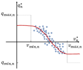
(a) Without fictional data points

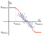
(b) With fictional data points

Figure 1: An illustration of the role of the fictional data points for DER at node $n$. Blue and orange points respectively represent true and fictional data points, while the dark red curves are instances of learned equilibrium functions. Adding fictional data points helps the equilibrium function reach maximum reactive power compensation capability when voltage exceeds the limits.

Remark V.3.

(Deep neural network parameterization of non-increasing function via gradient penalization): Though the single hidden layer neural network parameterization of (17) achieves universal approximation, it requires the “width” of the neural networks, i.e., $H$ to be sufficiently large. Instead, in certain situations, deeper neural networks could achieve better approximations than the shallower ones even if they are much narrower [28]. On the other hand, the structure-based restrictions enforced on the neural networks to guarantee monotonicity may in some cases restrict expressibility and lead to unsatisfactory approximation results [27]. To overcome the aforementioned challenges, we describe here a deep neural network parameterization approach by incorporating the monotonicity requirement as a penalization in the cost function of learning process. Suppose for each $n\in\mathcal{C}$, $\phi_{n}$ is parameterized by a deep neural network, and denote by $d\phi_{n}(v_{n})\in\mathbb{R}$ the (sub)gradient of $\phi_{n}$ with respect to $v_{n}$. The cost function in (15) is then replaced by

$$\sum_{k=1}^{K}|q_{n,k}^{\star}-\phi_{n}(v_{n,k}^{\star})|^{2}+\gamma_{n}\max(0,d\phi_{n}(v_{n,k}^{\star})),$$

where $\gamma_{n}>0$ is a tuning parameter. During implementation, one can gradually increase $\gamma_{n}$ until $\phi_{n}$ is verified to be non-increasing. $\bullet$

Remark V.4.

(On the comparison with existing reinforcement learning approaches): Recent literature has also investigated reinforcement learning (RL) approaches for learning stability guaranteed local Volt/Var controllers, e.g., [12, 13]. However, due to the lack of communication in the training phase, the cost function that the whole system seeks to minimize in such settings can only be separable, i.e., the summation of all the local cost functions at each node. Therefore, these approaches generally can not cope with cost functions like (3), which shows coupling among nodes. In contrast, since our approach only uses off-line collected data, any type of cost function could in principle be considered when solving the ORPF problem (6). $\bullet$

VI Numerical tests

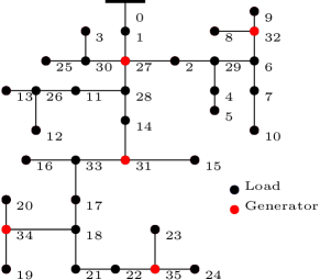
Figure 2: The IEEE 37-bus feeder.

We conduct case studies on the IEEE 37-bus feeder. We omit regulators, incorporate five solar generators, and convert it to its single-phase equivalent, see Fig. 2. The feeder has 25 buses with non-zero load, and the five solar generators are the DERs participating in reactive power compensation.

Real-world dataset. We extract minute-based load and solar generation data for June 1, 2018 from the Pecan Street dataset [29], and the first 75 non-zero load buses from the dataset are aggregated every 3 loads and normalized to obtain 25 load profiles. Similarly, we obtain 5 solar generation profiles for the active power of DERs. The normalized load profiles for the 24-hour period are scaled so that 97% of the total load duration curve coincides with the total nominal load. This scaling results in a peak aggregate load being 1.1 times the total nominal load. We synthesize reactive loads by scaling active demand to match the power factors of the IEEE 37-bus feeder. Fig. 3 shows the total demand and solar generation across the feeder.

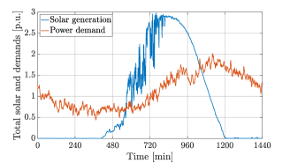
Figure 3: Minute-based data for the total (feeder-wise) solar power generation and active power demand.

ORPF problem and training setups. We consider the cost function in (6a) to be

$$f(\mathbf{q}_{\mathcal{C}}) =\alpha\underbrace{\|\mathbf{v}(\mathbf{q}_{\mathcal{C}})-\mathbf{1}\|}_{\text{\char 172}}+(1-\alpha)\underbrace{\ell(\mathbf{q}_{\mathcal{C}})}_{\text{\char 173}},$$

where ① and ② correspond to the minimization of voltage deviations and power losses, respectively, and the parameter $\alpha$ trades-off those two objectives. We assume the 5 DERs have uniform generation capabilities, precisely, $\mathbf{q}_{\max}=0.4\cdot\mathbf{1}$ MVAR and $\mathbf{q}_{\min}=-\mathbf{q}_{\max}$. The voltage limit vectors are set to $\mathbf{v}_{\max}=1.03\cdot\mathbf{1}$ p.u. and $\mathbf{v}_{\min}=0.97\cdot\mathbf{1}$ p.u. We use the Matlab CVX toolbox [30] to solve the ORPF problem (6). Although we utilize the linearized power flow equation (8b) for technical analysis, here we instead use Matpower [31] to compute the solution of the AC power flow equation so that the tests are more practical. We add the fictional data points to the obtained dataset as described in Remark V.2 with $\underline{K}=\overline{K}=700$, which results in a total of $2840$ data points for each DER. We implement the neural network approach according to Proposition V.1 using TensorFlow 2.7.0 and conduct the training process in Google Colab with a single TPU with 32 GB memory. The number of episodes and the number of neurons $H$ are 2000 and 1000, respectively, and the neural networks are trained using the Adam optimizer [32] with the learning rate initialized at 0.005 and decays every 500 steps with a base of 0.5.

Fig. 4 plots the learned equilibrium function along with the exact optimal solutions to the ORPF problem (6) for the DER at node 34 with $\alpha=\frac{2}{7}$. In contrast to the cases in which no fictional data points are added in the learning process, the learned equilibrium function with fictional data points reaches maximum reactive power compensation capability when voltage exceeds the limits. To guarantee the convergence of the non-incremental algorithm, i.e., $\epsilon=1$, one needs to further enforce an additional slope constraint (14) on the learned equilibrium functions, cf. Remark IV.4. Fig. 5 further shows that this additional slope constraint leads to larger approximation errors of the learned equilibrium functions in fitting the dataset (we do not consider the fictional data points here to exclude the possible impact of them for fairness), and thus degrades the optimality of system performance.

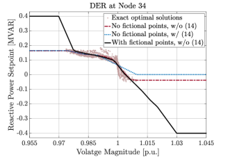
Figure 4: The black solid curve is the learned equilibrium function with fictional data points considered. The blue dotted and red dashdotted curves are respectively learned equilibrium functions with and without incorporating the additional slope constraint (14) when no fictional data points are added in the learning process. The comparison between black solid and red dashed curves illustrates the role of fictional data points in learning equilibrium functions. The former reaches the maximum reactive power compensation capability when the voltage exceeds the limits, while the latter does not. The comparison between blue dotted and red dashdotted curves instead shows the limitations of using non-incremental algorithms as they achieve worse fitting performance because of the additional slope constraint (14).

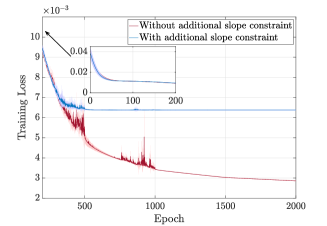
Figure 5: Comparison of training loss with and and without the additional slope constraint (14) on the equilibrium functions as described in Remark IV.4. The mean and standard deviations are evaluated based on 5 random seeds. This additional slope constraint leads to larger approximation error of the learned equilibrium functions in fitting the data points.

Simulation results. We run the following simulations using the learned equilibrium functions for the case $\alpha=\frac{2}{7}$ with fictional data points considered and assume that $\mathbf{q}_{\mathcal{C}}(0)=\mathbf{0}$. We first verify the convergence properties of the proposed reactive power update rule (7) stated in Proposition IV.2. Consider the scenario where load-generation profiles are fixed, Fig. 6 reports the evolution of the DERs’ reactive power setpoints using load-generation profiles of the 795-th minute and consider 120 iterations of (7). For $\epsilon=0.1$, the reactive power setpoint trajectories converge to their final values, cf. Fig. 6(a), while the case that $\epsilon=1$ fails, cf. Fig. 6(b). This is consistent with the sufficient condition $0<\epsilon<\min\{1,\frac{2}{(\|\mathbf{X}\|L+1)^{2}}\}=0.3691$ derived in Proposition IV.2.

Next, we test the proposed data-based control method in a scenario where load-generation profiles are time-varying. Specifically, we obtain load-generation profiles by randomly perturbing the consumption data used to learn the equilibrium functions. This can be interpreted as having the data from the dataset prescribing a day-ahead forecast, whereas their random perturbation act as the true realization of the load-generation scenarios. These loads and generations are minute-based and we consider 120 iterations of (7) per minute with $\epsilon=0.1$. Fig. 7 compares the evolution of minimum voltages and cost increases w.r.t. ORPF approach under the proposed data-based control method, linear droop control method, and the case where no control action is taken. Specifically, we adopt the linear droop control design from [3, 7] as

$$q_{n}(t+1)=\begin{cases}q_{\max,n}&v_{n}(t)\leq v_{\min,n},\\ q_{\min,n}&v_{n}(t)\geq v_{\max,n},\\ -c_{n}(v_{n}(t)\!-\!v_{\min,n})\!+\!q_{\max,n}&\text{otherwise},\end{cases}$$

where $c_{n}=\frac{q_{\max,n}-q_{\min,n}}{v_{\max,n}-v_{\min,n}}$. In contrast to the uncontrolled case, the proposed data-based control as well as linear droop control methods both keep the voltages within the desired voltage region, while the former significantly reduces the cost compared to the latter. To further illustrate the effectiveness and advantages of the proposed data-based control method, Table I summarizes the comparison results of the proposed data-based control method against the linear droop control method and the case where no control action is taken for different values of $\alpha$. It can be observed that the proposed data-based control method outperforms the linear droop control method for all cases.

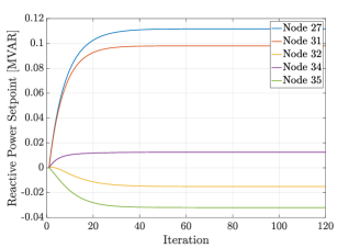
(a) $\epsilon=0.1$

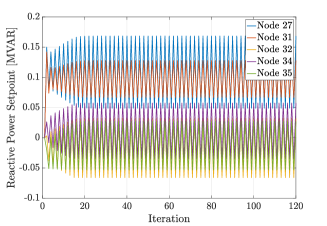
(b) $\epsilon=1$

Figure 6: Evolution of reactive power setpoints under the proposed reactive power update rule (7) with (a) $\epsilon=0.1$ and (b) $\epsilon=1$, where we use the power data profiles of the 795-th minute and consider 120 iterations. This verifies the sufficient condition $0<\epsilon<\min\{1,\frac{2}{(\|\mathbf{X}\|L+1)^{2}}\}=0.3691$ in Proposition IV.2 to ensure global asymptotic stability.

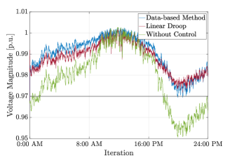
(a) Minimum voltages

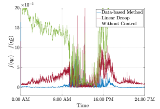
(b) Cost increases

Figure 7: Evolution of the (a) minimum voltages and (b) cost increases w.r.t. the ORPF approach of the IEEE 37-bus network under the proposed data-based, linear droop, and without control methods. For all minute-based data profiles, the ORPF problem is always feasible and thus the voltages under the ORPF approach are always within limits and $\mathbf{q}_{\mathcal{C}}^{\star}$ always exists.

TABLE I: Relative increase of total cost during evolution w.r.t. the ORPF solution

$\alpha$	Data-based	Linear Droop	Without Control
$0$	$\mathbf{4.94\%}$	$30.66\%$	$25.31\%$
$1/3$	$\mathbf{1.14\%}$	$8.15\%$	$52.35\%$
$1/2$	$\mathbf{6.16\%}$	$28.33\%$	$96.13\%$
$2/3$	$\mathbf{11.85\%}$	$49.99\%$	$137.52\%$
$1$	$\mathbf{63.86\%}$	$200.22\%$	$420.71\%$

Discussion. Our simulation results above validate the improved performance of the proposed data-based method compared to the linear droop control method for different control goals. In fact, apart from considering the minimization of voltage deviations and power losses, our framework allows the users to consider any other type of cost functions, depending on specific control goals, to learn purely local controllers that steer system operating points to approximated ORPF solutions. However, as one can observe in Table I, different cost functions may result in very different optimality gaps between the proposed data-based method and the ORPF approach. Since the dataset we construct only maps the local voltage to the local optimal reactive power setpoint, it is possible that one fixed voltage corresponds to multiple optimal reactive power setpoints. On the other hand, it is also possible that the optimal solution pairs are not so close to the non-increasing shape as we require the equilibrium functions to be. We refer to these phenomena as data inconsistency. We note that different selections of cost function significantly influence the data inconsistency, and thus leads to very different optimality gaps. For example, as Table I suggests, the data becomes significantly more inconsistent when the minimization of voltage deviations takes a more important role in the cost function. As part of our follow-up work, we plan to include other available local information to alleviate the data inconsistency challenge, e.g., prevailing (re)active power injections as additional inputs of the equilibrium function. Another important observation is that, although the ORPF approach strictly guarantees that the voltages are within limits, our approach does not. For instance, for the case $\alpha=0$, the voltage nadir during evolution under the proposed data-based method slightly violates the voltage limits. The reason is that when $\alpha$ is very small, many of the optimal solutions given by the ORPF problem lie on the boundary of the voltages limits. Since the local surrogates only provide approximations of the optimal solutions, the actual converged voltages can easily go out of limits in such situations. On the other hand, as pointed out in [10], purely local control strategies generally have no guarantee on desired regulation, in the sense that the equilibrium $\mathbf{q}_{\mathcal{C}}^{\sharp}$ of (8) could result in a $\mathbf{v}(\mathbf{q}_{\mathcal{C}}^{\sharp})\notin[\mathbf{v}_{\min},\mathbf{v}_{\max}]$, even if there indeed exists $\mathbf{q}_{\mathcal{C}}$ such that $\mathbf{v}(\mathbf{q}_{\mathcal{C}})\in[\mathbf{v}_{\min},\mathbf{v}_{\max}]$.

VII Conclusions

We have presented a data-driven framework to design local Volt/Var controllers capable of steering a power distribution network towards efficient network configurations. Building on the idea of learning local surrogates that map local voltages to reactive power setpoints that approximate the ORPF solution, we have proposed a local control update scheme and identified conditions on surrogates and control parameters so that the reactive power point converges in a global asymptotic sense. By constructing a labeled dataset of ORPF solutions with different load and generation profiles, we have trained neural networks whose resulting parameterized functions meet the conditions on surrogates by design to fit the dataset. We have shown in AC power flow simulation tests that the proposed framework guarantees the voltage stability and significantly reduces operation cost compared to prevalent local control approaches. Future research directions include enhancing data consistency by making use of other local information in building the dataset, reducing the optimality gap during the learning process, and extending the proposed framework to more general scenario where we take advantage of communication among neighboring agents.

Appendix A Technical Lemmas

Lemma A.1.

(Bauer and Fike Theorem [33, Corollary 6.3.4]): Let $\mathbf{A},\mathbf{E}\in\mathbb{R}^{n\times n}$ with $\mathbf{A}$ normal. If $\hat{\lambda}$ is an eigenvalue of $\mathbf{A}+\mathbf{E}$, then there exists an eigenvalue $\lambda$ of $\mathbf{A}$ such that $|\hat{\lambda}-\lambda|\leq\|\mathbf{E}\|$.

Lemma A.2.

(Positive semidefiniteness of $\mathbf{X}\mathbf{M}$ and upper bound of $\|\mathbf{X}\mathbf{M}\|$): The matrix $\mathbf{X}\mathbf{M}$ is positive semidefinite. Moreover, it holds

$$\|\mathbf{X}\mathbf{M}\|\leq\|\mathbf{X}\|L.$$

Proof.

Let $(\lambda_{i},\boldsymbol{\xi}_{i})$ be a left eigenpair for $\mathbf{X}\mathbf{M}$. Then, $(\lambda_{i},\boldsymbol{\xi}_{i}\mathbf{X}^{\frac{1}{2}})$ is a left eigenpair for the symmetric matrix $\mathbf{X}^{\frac{1}{2}}\mathbf{M}\mathbf{X}^{\frac{1}{2}}\succeq 0$. Indeed,

$$\boldsymbol{\xi}_{i}\mathbf{X}^{\frac{1}{2}}\mathbf{X}^{\frac{1}{2}}\mathbf{M}\mathbf{X}^{\frac{1}{2}} =\boldsymbol{\xi}_{i}\mathbf{X}\mathbf{M}\mathbf{X}^{\frac{1}{2}}=\lambda_{i}\boldsymbol{\xi}_{i}\mathbf{X}^{\frac{1}{2}}.$$

Therefore, $\mathbf{X}\mathbf{M}$ is positive semidefinite as well. Also, it holds that

$$\|\mathbf{X}\mathbf{M}\|\leq\|\mathbf{X}\|\|\mathbf{M}\|\leq\|\mathbf{X}\|L,$$

which completes the proof. ∎

Lemma A.3.

(Universal approximation to Lipschitz function using ReLU activation function): Consider the neural network (17). For any Lipschitz function $g:\mathbb{R}\rightarrow\mathbb{R}$ and given any compact domain $\mathcal{X}\in\mathbb{R}$ and $\eta>0$, there exist $H$, $w_{h}$, $b_{h}$, and $\beta$ such that $|\mathsf{N}(x)-g(x)|\leq\eta$ for all $x\in\mathcal{X}$.

Proof.

Given a compact domain $\mathcal{X}$ of the form $\underline{x}\leq x\leq\overline{x}$, consider an equispaced partition of $\mathcal{X}$ into $H$ segments, with the length of each segment being $s=\frac{\overline{x}-\underline{x}}{H}$. Let $\beta=g(\underline{x})$, $b_{h}=\underline{x}+(h-1)s$ and $\sum_{k=1}^{h}w_{k}=\frac{g(\underline{x}+hs)-g(\underline{x}+(h-1)s)}{s}$ for $h\in\{1,2,\dots,H\}$. It follows that

$$|\mathsf{N}(x)-g(x)|\leq L_{g}s,$$

where $L_{g}$ is the Lipschitz constant of $g$. Hence, by setting $H\geq\frac{L_{g}(\overline{x}-\underline{x})}{\eta}=O(1/\eta)$, it holds that $|\mathsf{N}(x)-g(x)|\leq L_{g}s\leq\eta$ for all $x\in\mathcal{X}$. This completes the proof. ∎

References

- [1] “IEEE standard for interconnection and interoperability of distributed energy resources with associated electric power systems interfaces,” IEEE Std 1547-2018 (Revision of IEEE Std 1547-2003), pp. 1–138, 2018.
- [2] E. Dall’Anese, H. Zhu, and G. B. Giannakis, “Distributed optimal power flow for smart microgrids,” IEEE Transactions on Smart Grid, vol. 4, no. 3, pp. 1464–1475, 2013.
- [3] G. Cavraro and R. Carli, “Local and distributed voltage control algorithms in distribution networks,” IEEE Transactions on Power Systems, vol. 33, no. 2, pp. 1420–1430, 2017.
- [4] E. Dall’Anese and A. Simonetto, “Optimal power flow pursuit,” IEEE Transactions on Smart Grid, vol. 9, no. 2, pp. 942–952, 2018.
- [5] G. Qu and N. Li, “Optimal distributed feedback voltage control under limited reactive power,” IEEE Transactions on Power Systems, vol. 35, no. 1, pp. 315–331, 2020.
- [6] M. K. Singh, S. Taheri, V. Kekatos, K. P. Schneider, and C. C. Liu, “Joint grid topology reconfiguration and design of Watt-VAR curves for DERs,” in IEEE Power & Energy Society General Meeting, (Denver, CO, USA), July 2022. To appear.
- [7] K. Turitsyn, P. Sulc, S. Backhaus, and M. Chertkov, “Options for control of reactive power by distributed photovoltaic generators,” Proceedings of the IEEE, vol. 99, no. 6, pp. 1063–1073, 2011.
- [8] H. Zhu and H. J. Liu, “Fast local voltage control under limited reactive power: Optimality and stability analysis,” IEEE Transactions on Power Systems, vol. 31, no. 5, pp. 3794–3803, 2015.
- [9] X. Zhou, M. Farivar, Z. Liu, L. Chen, and S. H. Low, “Reverse and forward engineering of local voltage control in distribution networks,” IEEE Transactions on Automatic Control, vol. 66, no. 3, pp. 1116–1128, 2021.
- [10] S. Bolognani, R. Carli, G. Cavraro, and S. Zampieri, “On the need for communication for voltage regulation of power distribution grids,” IEEE Transactions on Control of Network Systems, vol. 6, no. 3, pp. 1111–1123, 2019.
- [11] X. Chen, G. Qu, Y. Tang, S. H. Low, and N. Li, “Reinforcement learning for selective key applications in power systems: Recent advances and future challenges,” IEEE Transactions on Smart Grid, 2022. To appear.
- [12] W. Cui, J. Li, and B. Zhang, “Decentralized safe reinforcement learning for inverter-based voltage control,” Electric Power Systems Research, vol. 211, p. 108609, 2022.
- [13] Y. Shi, G. Qu, S. H. Low, A. Anandkumar, and A. Wierman, “Stability constrained reinforcement learning for real-time voltage control,” in American Control Conference, (Atlanta, GA), pp. 2715–2721, June 2022.
- [14] X. Pan, T. Zhao, M. Chen, and S. Zhang, “DeepOPF: A deep neural network approach for security-constrained DC optimal power flow,” IEEE Transactions on Power Systems, vol. 36, no. 3, pp. 1725–1735, 2021.
- [15] A. S. Zamzam and K. Baker, “Learning optimal solutions for extremely fast AC optimal power flow,” in IEEE Int. Conf. on Communications, Control, and Computing Technologies for Smart Grids, (Tempe, AZ, USA), Nov. 2020.
- [16] D. Owerko, F. Gama, and A. Ribeiro, “Optimal power flow using graph neural networks,” in IEEE Int. Conf. on Acoustics, Speech and Signal Processing, (Barcelona, Spain), pp. 5930–5934, 2020.
- [17] M. K. Singh, S. Gupta, V. Kekatos, G. Cavraro, and A. Bernstein, “Learning to optimize power distribution grids using sensitivity-informed deep neural networks,” in IEEE Int. Conf. on Communications, Control, and Computing Technologies for Smart Grids, (Tempe, AZ, USA), Nov. 2020.
- [18] M. K. Singh, V. Kekatos, and G. B. Giannakis, “Learning to solve the AC-OPF using sensitivity-informed deep neural networks,” IEEE Transactions on Power Systems, vol. 37, no. 4, pp. 2833–2846, 2022.
- [19] S. Karagiannopoulos, P. Aristidou, and G. Hug, “Data-driven local control design for active distribution grids using off-line optimal power flow and machine learning techniques,” IEEE Transactions on Smart Grid, vol. 10, no. 6, pp. 6461–6471, 2019.
- [20] P. S. Torre and P. Hidalgo-Gonzalez, “Decentralized optimal power flow for time-varying network topologies using machine learning,” Electric Power Systems Research, vol. 212, p. 108575, 2022.
- [21] G. Cavraro, Z. Yuan, M. K. Singh, and J. Cortés, “Learning local Volt/Var controllers towards efficient network operation with stability guarantees,” in IEEE Conf. on Decision and Control, (Cancun, Mexico), Dec. 2022. To appear.
- [22] A. M. Kettner and M. Paolone, “On the properties of the compound nodal admittance matrix of polyphase power systems,” IEEE Transactions on Power Systems, vol. 34, no. 1, pp. 444–453, 2019.
- [23] K. C. Border, Fixed Point Theorems with Applications to Economics and Game Theory. Cambridge, UK: Cambridge University Press, 1985.
- [24] M. Farivar, X. Zhou, and L. Chen, “Local voltage control in distribution systems: An incremental control algorithm,” in IEEE Int. Conf. on Communications, Control, and Computing Technologies for Smart Grids, (Miami, FL, USA), pp. 732–737, Nov. 2015.
- [25] H. Daniels and M. Velikova, “Monotone and partially monotone neural networks,” IEEE Transactions on Neural Networks, vol. 21, no. 6, pp. 906–917, 2010.
- [26] A. Wehenkel and G. Louppe, “Unconstrained monotonic neural networks,” in Conference on Neural Information Processing Systems, vol. 32, (Vancouver, Canada), pp. 1543–1553, Dec. 2019.
- [27] X. Liu, X. Han, N. Zhang, and Q. Liu, “Certified monotonic neural networks,” in Conference on Neural Information Processing Systems, vol. 33, (Vancouver, Canada), pp. 15427–15438, Dec. 2020.
- [28] I. Safran and O. Shamir, “Depth-width tradeoffs in approximating natural functions with neural networks,” in International Conference on Machine Learning, (Sydney, Australia), pp. 2979–2987, Aug. 2017.
- [29] “Dataport: The world’s largest energy data resource,” Pecan Street Inc, 2015. Available at https://dataport.pecanstreet.org/.
- [30] M. Grant and S. Boyd, “CVX: Matlab software for disciplined convex programming, version 2.1,” Mar. 2014. Available at http://cvxr.com/cvx.
- [31] R. D. Zimmerman, C. E. Murillo-Sánchez, and R. J. Thomas, “Matpower: Steady-state operations, planning and analysis tools for power systems research education,” IEEE Transactions on Power Systems, vol. 26, no. 1, pp. 12–19, 2011.
- [32] D. P. Kingma and J. Ba, “Adam: A method for stochastic optimization,” in International Conference on Learning Representations, (San Diego, CA, USA), May 2015.
- [33] R. A. Horn and C. R. Johnson, Matrix Analysis. Cambridge University Press, 2012.