Anomalous and axial $Z^{\prime}$ contributions to $g-2$

Abstract

We study the effects of an anomalous $Z^{\prime}$ boson on the anomalous magnetic moment of the muon $(g-2)$, and especially the impact of its axial coupling. We mainly evaluate the negative contribution to $(g-2)$ of such couplings at one-loop and look at the anomalous couplings generated at two loops. We find areas of the parameter space, where the anomalous contribution becomes comparable and even dominant compared to the one-loop contribution. We show that in such cases, the cutoff of the theory is sufficiently low, so that new charged fermions can be found in the next round of collider experiments. We comment on the realization of such a context in string theory orientifolds.

1 Introduction

The Standard Model (SM) is the most accurate physical theory ever made. It predicts, among others, the anomalous magnetic moment of the muon to be Aoyama:2020ynm (see also other SM g-2 1 ; other SM g-2 2 ; other SM g-2 3 ; other SM g-2 4 ; other SM g-2 5 ; other SM g-2 6 ; other SM g-2 7 ; other SM g-2 8 ; other SM g-2 9 ; other SM g-2 10 ; other SM g-2 11 ; other SM g-2 12 ; other SM g-2 13 ; other SM g-2 14 ; other SM g-2 15 ; other SM g-2 16 ; other SM g-2 17 ; other SM g-2 18 ; other SM g-2 19 ; other SM g-2 20 ; other SM g-2 21 ; other SM g-2 22 ; other SM g-2 23 ; Crivellin:2020zul ; other SM g-2 24 ; other SM g-2 25 )

$$a^{\mathrm{SM}}_{\mu}=$116\,591\,810(43)\text{\times}{10}^{-11}\text{\,}$~{}.$$ (1.1)

In comparison, the latest experimental measured value of the Fermilab National Accelerator Laboratory (FNAL) Muon $g-2$ Experiment (E$989$) Abi:2021gix

$$a^{\mathrm{exp}}_{\mu}(\mathrm{FNAL})=$116\,592\,061(41)\text{\times}{10}^{-11}\text{\,}$~{},$$ (1.2)

with a precision of $(0.35\;\mathrm{ppm})$, gives

$$a_{\mu}^{\mathrm{exp}}-a_{\mu}^{\mathrm{SM}}=$251(59)\text{\times}{10}^{-11}\text{\,}$~{}.$$ (1.3)

The discrepancy is roughly of magnitude $4.2\sigma$ and although not fully incompatible with the SM, it indicates the possibility of “new physics” contributions Jackiw:1972jz ; Bardeen:1972vi ; Leveille:1977rc ; Holdom:1985ag ; Kukhto:1992qv ; AK ; Armillis:2008bg ; Pospelov:2008zw ; Freitas:2014pua ; Davoudiasl:2014kua ; Dorsner:2016wpm ; 1511.07447 ; 1712.09360 ; Kamada:2018zxi ; Crivellin:2018qmi ; Liu:2018xkx ; Dutta:2018fge ; Han:2018znu ; 1906.11297 ; CarcamoHernandez:2019ydc ; Jho:2019cxq ; Endo:2019bcj ; Badziak:2019gaf ; Hiller:2019mou ; Bauer:2019gfk ; Gardner:2019mcl ; Cornella:2019uxs ; Crivellin:2019mvj ; Abdullah:2019ofw ; Criado:2019tzk ; Dutta:2020scq ; Yang:2020bmh ; Bigaran:2020jil ; Dorsner:2020aaz ; Botella:2020xzf ; Jana:2020pxx ; CarcamoHernandez:2020pxw ; Haba:2020gkr ; Calibbi:2020emz ; Arbelaez:2020rbq ; Chen:2020jvl ; Hati:2020fzp ; Jana:2020joi ; Chen:2020tfr ; Chun:2020uzw ; Li:2020dbg ; Banerjee:2020zvi ; Antoniadis:2021mqz ; Hernandez:2021tii ; Capdevilla:2021kcf ; Barman:2021xeq ; Hammad:2021mpl ; Chowdhury:2021tnm ; Yu:2021suw ; Athron:2021iuf ; Cadeddu:2021dqx ; Bodas:2021fsy ; Coy:2021wfs ; Li:2021koa ; Li:2021lnz ; Han:2021gfu ; Cao:2021lmj ; Botella:2022rte ; Kriewald:2022erk ; DAlise:2022ypp ; Panda:2022kbn ; Chowdhury:2022jde ; Anastasopoulos:2022wob ; Crivellin:2021rbq . Some works tried to reconciliate the $g-2$ excess with dark matter constraints Arcadi:2021zdk , $B-$anomalies Calibbi:2021vcq or the $M_{W}$ curiosity Arcadi:2022dmt . In searching for new physics, one possible and rather generic scenario involves the extension of the SM with an additional massive gauge boson $Z^{\prime}$. This gauge boson may couple to all or some SM fields (fermions and the Higgs) and presents one of the most popular scenarios for physics beyond the SM at the LHC. Among all the possible extensions of the SM, the introduction of an additional gauge group is also one of the most motivated. It can for instance serve as a mediator between the dark sector and the visible world, in order to explain the dark matter production in the early Universe Arcadi:2013qia and appear in unified theories Mambrini:2015vna .

In this paper, we study an extension of the SM with a more general type of $Z^{\prime}$ bosons, which are superficially anomalous. With the term “superficially anomalous” we refer to the fact that the associated gauge symmetry is anomaly-free in the ultraviolet (UV) fundamental theory, but appears anomalous in the low-energy effective field theory, that is obtained after integrating out an anomalous set of heavier states ABDK . Such gauge symmetries are typically associated with gauged baryon, lepton number, or some Peccei-Quinn symmetry. Therefore, they are crucial for realizing the SM global symmetries and the associated constraints on baryon and lepton number conservation.

Depending on the realization of the UV theory, the interpretation of the appearance of low-energy anomalous gauge symmetries can be different. In string theory realizations, such gauge symmetries are broken by the Stückelberg mechanism tied to the Green-Schwarz-type cancellation of their anomalies, and the associated gauge fields become massive ABDK ; Kiritsis:2003mc ; au1 ; AKR ; PA2 ; MambriniGS ; CIK ; PA ; Anastasopoulos:2008jt ; Armillis:2008vp ; Accomando:2016sge ; Dudas:2012pb . Additional generalized Chern-Simons terms (GCS) appear in the low energy theory to cure the model of all types of mixed anomalies, ABDK ; AKT . Such anomalous $U(1)$’s in the effective theory, can also be interpreted as a UV completion in the context of QFT ABDK ; NC . The $U(1)$ gauge boson obtains a mass from one or more Higgs scalars, whereas the Higgs mechanism gives masses to an anomalous subset of fermions. In the limit where the anomalous subset of fermions and the physical Higgses become heavy, the low-energy theory is that of anomalous $U(1)$’s, with the Stückelberg scalar being the phase of the Higgs ABDK .

The difference between anomalous and non-anomalous $Z^{\prime}$s lies in a set of special, anomaly-related three-gauge-boson couplings which are not present in the non-anomalous case AK ; Armillis:2008bg ; CIK ; ABDK ; PA ; Anastasopoulos:2008jt ; Armillis:2008vp ; Accomando:2016sge and can have observable consequences on low energy phenomenology CIK ; Anastasopoulos:2008jt ; Dudas:2012pb . Note that such effective theories can appear anomalous or non-anomalous at different scales. Therefore, studying the phenomenological consequences of such models is exciting and relevant.

Adding abelian factors that couple to some or all of the SM fields produces very popular extensions of the SM. In this category, we have lepton-flavor violating $Z^{\prime}$, leptophilic $Z^{\prime}$s (abelian factors that couple only to leptons), $U(1)_{T3R}$ (an abelian field that couples to all right-handed fermions of the SM), etc. The non-anomalous versions of these constructions have been extensively studied. It becomes then interesting to look at the phenomenological consequences of their anomalous versions. It is also worth mentioning that studying anomalous $U(1)$s is very timely due to upcoming experiments. The Forward Physics Facility (FPF) is planned to operate near the ATLAS interaction point during the LHC high-luminosity era FPF . It will investigate long-lived particles that might escape the apparatus, and new abelian gauge fields have a prominent position in these searches.

The present paper aims to evaluate the contribution of a $Z^{\prime}$ boson to the $g-2$ of the muon including the possibility of anomalous couplings AK ; Armillis:2008bg . In particular, we focus on the leading contribution of the anomalous three-gauge-boson coupling to the $g-2$, comparing it to the contribution evaluated in the non-anomalous case. The anomalous couplings being generated at one-loop, the difference in the $g-2$ appears at two-loop order. We focus on the most straightforward class of models, in which we extend the SM with a single additional anomalous abelian $U(1)$ gauge symmetry, an associated axion, and generalized Chern-Simons terms necessary to cancel all the possible anomalies. After electroweak symmetry breaking, we obtain the SM fields plus an additional massive $Z^{\prime}$ whose non-minimal couplings are entirely determined by the anomaly cancellation conditions. In a sense, any phenomenological constraints on the couplings give direct information on the content of the UV completion due to anomaly matching, and vice-versa.

Results and outlook

After parametrizing the anomalous three-gauge-boson couplings, we evaluate their contribution to the $g-2$ of the muon, first presented in general terms without using any assumption for the values of the parameters of our model. Then, we proceed to a phenomenological analysis, where we consider a low-mass $Z^{\prime}$ model (with $m_{Z^{\prime}}\ll m_{Z}$), and we show that the anomalous contribution can dominate the two-loop diagrams while lying within the error zone of the discrepancy (1.3).

Indeed, in the leading one-loop contribution of a $Z^{\prime}$ to the $g-2$, the axial and vectorial parts compete with a negative relative sign. Consequently, regions in the parameter space exist where the one-loop contribution can be highly suppressed, becoming subdominant compared to higher-order contributions. In such a case, the anomalous (two-loop) diagrams that depend on the anomaly become dominant. The anomalous contributions can be considered a litmus test for higher energy physics that filters to low energy via the anomalies.

We then calculate the anomalous contribution to the $g-2$, performing numerical integrations for a specific range of the mass of the $m_{Z^{\prime}}$ and the couplings and compare the anomalous contribution to the non-anomalous one.

• At one-loop, because the vectorial and axial couplings of the muon to an anomalous $Z^{\prime}$ can be arbitrary and are not constrained by anomaly cancellation, the result is less constrained than non-anomalous models.

• The anomalous $U(1)$ has an extra anomalous cubic coupling which depends on the overall anomaly, a property of the theory in the UV regime. Any chiral fermion of the fundamental theory charged under the anomalous abelian factors contributes to the anomalous coupling. Therefore, apart from the SM fermions, the heavier fermions that are integrated out and are charged under the anomalous $Z^{\prime}$, can give a very large value to this coupling, with significant phenomenological consequences. This contribution can be comparable to the one-loop effects. We show that it is much more significant to the standard non-anomalous $Z^{\prime}$ two-loop contributions.

• We also show that in the interesting cases, the cutoff of the theory is in the tens of TeV range, implying that there may be charged fermions to be discovered in the next generation of colliders.

In this paper, we evaluate the anomalous contribution to the $g-2$ of fermions, and we provide generic formulas as functions of the mass, the couplings of the $Z^{\prime}$, and the anomalies. Some numerical examples show that the axionic and GCS contributions are leading compared to the fermionic triangle-loop.

We then explore some phenomenologically interesting models where the anomalous $Z^{\prime}$ couples to the muon and tau (and maybe to other heavy fermions) but not to the electron, to avoid experimental constraints on the couplings and masses of the anomalous $Z^{\prime}$.

Finally, we investigate whether an anomalous leptonic abelian factor that couples to the muon and tau and not to the electron can be found in semi-realistic D-brane configurations. We analyze models with three, four, five, and more D-branes stacks, and we conclude that this scenario can be observed only in the six D-brane stack models.

The paper is organized as follows. In Sec. 2 we present our EFT model, i.e., the SM extended with an anomalous $U(1)$ and an axion. We explain our methodology to compute the anomalous three-gauge boson coupling diagrams in Sec. 3 and evaluate analytically the contribution of the anomalous coupling to the $(g-2)$ of the muon in Sec. 4. We then lead a complete numerical analysis on the corresponding parameter space in Sec. 5. Finally, Sec. 6 is devoted to a discussion about D-brane realizations of the SM, which could accommodate anomalous $U(1)$s with the properties mentioned in the previous sections.

In the appendixes, we provide some of the necessary ingredients of our model and give some more details on our computations.

2 Extending the Standard Model with a single anomalous $U(1)_{A}$ and an axion

In this section, we introduce the effective theory of an extension of the SM with a single (massive) $U(1)_{A}$ and an associated axion. This theory can be obtained as an effective theory, from a class of theories described in appendix A where first we describe the generic properties. In In subsection A.1, we provide values to obtain a low mass anomalous $Z^{\prime}$ model, which will be used in the later phenomenological part of this work.

2.1 Building the Lagrangian

When one extends the Standard Model by an extra “anomalous" $U(1)_{A}$ and an axion $a$. The charges of the SM fields under this extra $U(1)_{A}$ are assumed to be family-non-universal. The transformations of the SM fields under this extra gauge symmetry, as well as the hypercharge symmetry, are

$$\begin{array}[]{llllllllll}&A^{\mu}&\to&A^{\mu}+\partial^{\mu}\varepsilon,&{}{}{}&Y^{\mu}&\to&Y^{\mu}+\partial^{\mu}\zeta,\\ &a&\to&a-M\varepsilon,&{}{}{}&\\ &\psi&\to&e^{ig_{A}q^{\psi-A}\varepsilon}\psi,&{}{}{}&\psi&\to&e^{ig_{Y}q^{\psi-Y}\zeta}\psi,\\ &H&\to&e^{ig_{A}q^{H-A}\varepsilon}H,&{}{}{}&H&\to&e^{ig_{Y}q^{H-Y}\zeta}H,\end{array}$$ (2.8)

where $M=g_{A}q^{S-A}V$ is the mass of the anomalous $U(1)_{A}$, $A^{\mu}$, and $\psi$ denotes all SM fermions collectively. $H$ is the SM Higgs doublet of the SM and ($\varepsilon$,$\zeta$) are the $U(1)_{A}$ and $U(1)_{Y}$ transformation parameters, respectively.

The charges of the SM fields are written

$$\begin{array}[]{llccccrrcccccc}&&&SU(3)&&SU(2)&&U(1)_{Y}&&U(1)_{A}&&\\ &Q^{i}_{L}&~{}:{}&{\bf 3}&&{\bf 2}&&1/6{}{}&&q_{i}^{Q-A}&&\\ &u_{R}^{i,c}&~{}:{}&\bar{\bf 3}&&{\bf 1}&&-2/3{}{}&&q_{i}^{u-A}&&\\ &d_{R}^{i,c}&~{}:{}&\bar{\bf 3}&&{\bf 1}&&1/3{}{}&&q_{i}^{d-A}&&\\ &L_{L}^{i}&~{}:{}&{\bf 1}&&{\bf 2}&&-1/2{}{}&&q_{i}^{L-A}&&\\ &l_{R}^{i,c}&~{}:{}&{\bf 1}&&{\bf 1}&&1{}{}&&q_{i}^{l-A}&&\\ &H&~{}:{}&{\bf 1}&&{\bf 2}&&1/2{}{}&&q^{H-A}&&\end{array}$$ (2.16)

with $i=1,2,3$ for the three SM families, and we use the hypercharge definition $Y=Q-T^{3}_{L}$. Assuming that the Yukawa terms are allowed by all symmetries, we obtain the constraints

$$\begin{array}[]{llllllll}\bar{Q}_{L}^{i}u_{R}^{j}H^{*}&{}{}{}&:&{}{}{}&-q_{i}^{Q-A}-q_{j}^{u-A}-q^{H-A}=0\\ \bar{Q}_{L}^{i}d_{R}^{j}H&&:&&-q_{i}^{Q-A}-q_{j}^{d-A}+q^{H-A}=0\\ \bar{L}_{L}^{i}l_{R}^{j}H&&:&&-q_{i}^{L-A}-q_{j}^{l-A}+q^{H-A}=0\end{array}$$ (2.20)

Therefore, only few charges remain free. However, this extension might suffer from mixed anomalies. For the generic charges, the anomaly-related traces are given below.

$$\begin{array}[]{llllllll}Tr[q_{Y}]=Tr[q_{Y}q_{Y}q_{Y}]=Tr[q_{Y}T_{SU(2/3)}^{a}T_{SU(2/3)}^{a}]&=0\\ Tr[q_{A}q_{Y}q_{Y}]=\sum_{i}\frac{q_{i}^{Q-A}}{6}+\frac{4q_{i}^{u-A}}{3}+\frac{q_{i}^{d-A}}{3}+\frac{q_{i}^{L-A}}{2}+{q^{l-A}_{i}{}{}}&=t_{AYY}\\ Tr[q_{Y}q_{A}q_{A}]=\sum_{i}(q_{i}^{Q-A})^{2}-2(q_{i}^{u-A})^{2}+(q_{i}^{d-A})^{2}-(q_{i}^{L-A})^{2}+(q_{i}^{l-A})^{2}{}{}&=t_{YAA}\\ Tr[q_{A}q_{A}q_{A}]=\sum_{i}6(q_{i}^{Q-A})^{3}+3(q_{i}^{u-A})^{3}+3(q_{i}^{d-A})^{3}+2(q_{i}^{L-A})^{3}+(q_{i}^{l-A})^{3}&=t_{AAA}{}{}{}\\ Tr[q_{A}T^{a}_{SU(2)}T^{a}_{SU(2)}]=\sum_{i}3q_{i}^{Q-A}+q_{i}^{L-A}{}{}{}{}{}{}{}{}{}{}{}{}{}{}{}{}{}{}{}{}{}{}{}{}{}{}{}&=T_{A,2}\\ Tr[q_{A}T^{a}_{SU(3)}T^{a}_{SU(3)}]=\sum_{i}2q_{i}^{Q-A}+q_{i}^{u-A}+q_{i}^{d-A}{}{}{}{}{}{}{}{}{}{}{}{}{}{}{}{}{}{}{}{}&=T_{A,3}\end{array}$$ (2.27)

where the traces are over all the SM fermions circulating in the anomalous loop and $T^{a}_{SU(2/3)}$ the generators of the non-abelian gauge groups of the SM. In our conventions, the $T^{a}_{SU(2/3)}$ normalization is $Tr[T^{a}_{i}T^{b}_{j}]=\delta^{ab}\delta_{ij}/2$ where $ij$ run over the different gauge groups, and $ab$ over the different generators of the relevant gauge groups. As we have already mentioned, these non-vanishing anomalies in the effective action are canceled via axionic and GCS terms, which appeared after integrating out the heavy fermions. The Lagrangian can then be written

$${\cal L} = {\cal L}_{\textrm{SM}}+{\cal L}_{\textrm{extra~{}fields}}$$ (2.28)

where ${\cal L}_{\textrm{SM}}$ is the SM Lagrangian and

$${\cal L}_{\textrm{extra~{}fields}} = -{1\over 4}F^{A}_{\mu\nu}F_{A}^{\mu\nu}+{1\over 2}(\partial_{\mu}a+MA_{\mu})^{2}+g_{A}q^{\psi-A}A_{\mu}\bar{\psi}\gamma^{\mu}\psi$$ (2.29)

$$+2ig_{A}q^{H-A}A^{\mu}H^{\dagger}\Big{(}\partial_{\mu}-ig_{2}{T^{\alpha}W^{\alpha}_{\mu}-ig_{Y}q^{H-Y}Y_{\mu}-{i\over 2}g_{A}q^{H-A}A_{\mu}}\Big{)}H$$

$$+{1\over 24\pi^{2}}a\Big{(}C_{YY}F_{Y}\wedge F_{Y}+C_{YA}~{}F_{Y}\wedge F_{A}+C_{AA}~{}F_{A}\wedge F_{A}+\sum_{i=2,3}D_{i}~{}Tr_{i}[G\wedge G]\Big{)}$$

$$+{1\over 24\pi^{2}}A\wedge Y\wedge\Big{(}E_{AY,A}F_{A}+E_{AY,Y}F_{Y}\Big{)}$$

$$+{1\over 24\pi^{2}}\sum_{i=2,3}Z_{i}~{}A\wedge Tr_{i}\Big{[}A\wedge(dA-{2\over 3}A\wedge A\Big{)}\Big{]}$$

where

$$F_{i}\wedge F_{j}={1\over 4}\varepsilon_{\mu\nu\rho\sigma}F_{i}^{\mu\nu}F_{j}^{\rho\sigma}\;\;\;,\;\;\;A_{i}\wedge A_{j}\wedge F_{k}\equiv{1\over 2}\varepsilon_{\mu\nu\rho\sigma}A_{i}^{\mu}A_{j}^{\nu}F_{k}^{\rho\sigma}$$ (2.30)

with $F_{X}^{\mu\nu}=\partial^{\mu}X^{\nu}-\partial^{\nu}X^{\mu}$ the field strength of the field $X_{\mu}$. Also, by $i=2,3$ we denote the non-abelian sectors of SU(2) and SU(3). $Tr_{i}$ is the appropriate non-abelian trace in the fundamental representation and $G$ stands for the non-abelian field strength. Note that the two last lines in (2.29) are the GCS terms for the abelian and abelian-non abelian factors, whereas GCS terms between the hypercharge $Y$ and the non-abelian factors vanish ABDK .

In the second line of (2.29) we have the minimal couplings of the anomalous $U(1)_{A}$ to the SM fields, fermions $\psi$ = quarks, leptons with charges $q^{\psi-A}$ and to the Higgs field $H$ with charge $q^{H-A}$ (see (2.16)). Notice the square $A^{\mu}A_{\mu}$ term from the Higgs coupling, which provides an extra contribution to the mass of the anomalous $U(1)_{A}$. We should also mention the presence of instanton-generated couplings between the fermions and the axion, which we omit here, as they will not be relevant for our calculation.

At 1-loop, the gauge symmetries are broken due to the anomalous diagrams, i.e., the non-vanishing traces of (2.27). Therefore, the effective theory is not invariant due to the triangle contributions of the low-energy fermions that give

$$\delta S_{\rm one-loop} = -{1\over 24\pi^{2}}\int\bigg{\{}\epsilon\Big{(}t_{AYY}F_{Y}\wedge F_{Y}+t_{YAA}F_{A}\wedge F_{Y}+{t_{AAA}}F_{A}\wedge F_{A}+T_{A,i}Tr[G_{i}\wedge G_{i}]\Big{)}$$ (2.31)

$$~{}~{}~{}~{}~{}~{}~{}~{}~{}~{}~{}+\zeta\Big{(}t_{YAA}F_{A}\wedge F_{A}+t_{AYY}F_{A}\wedge F_{Y}\Big{)}\bigg{\}}$$

where the coefficients are related to the low-energy charges via (2.27). We shall assume that such coefficients are generically non-zero.

Because of this, not only the extra $U(1)_{A}$ is anomalous, but also hypercharge has an anomaly, as testified by the terms in (2.31) that are proportional to $\zeta$. Of course, these anomalies should be canceled if we also include the anomalous variation of the tree level effective action in (2.29). Imposing anomaly cancellation gives (where $i=2,3$ for the non-abelian factors)

$$\delta S_{\textrm{one-loop}}+\delta S_{\rm extra~{}fields}=0~{}\to~{}\left\{\begin{array}[]{llllllll}MC_{YY}=-2{g_{A}g_{Y}^{2}}t_{AYY}&&MC_{YA}=-2{g_{A}^{2}g_{Y}}t_{YAA}\\ MC_{AA}=-{g_{A}^{3}}t_{AAA}&&2MD_{i}=-3Z_{i}=-6{g_{A}g_{i}^{2}}T_{A,i}\\ E_{AY,A}={g_{A}^{2}g_{Y}}t_{YAA}&&E_{AY,Y}={g_{A}g_{Y}^{2}}t_{AYY}\end{array}\right.~{}~{}~{}~{}~{}~{}~{}$$ (2.35)

The conditions (2.35) fix the coefficients of the axionic and the GCS terms in (2.29). Note that when there are at least two Stükelberg gauge fields and an analogous number of axions in the action, an extra gauge-invariant term involving the generalized Chern-Simons terms is available, ABDK ,

$${\cal L}_{inv}={1\over 2}\varepsilon_{\mu\nu\rho\sigma}(\partial^{\mu}a_{I}+M_{I}A_{I}^{\mu})(\partial^{\nu}a_{J}+M_{J}A_{J}^{\nu})({\mathbbm{d}}_{4}^{IJK}F^{\rho\sigma}_{A_{K}}+{\mathbbm{d}}^{IJ}_{5}F^{\rho\sigma}_{Y})$$ (2.36)

The ${\mathbbm{d}}_{4,5}$ are constants, which we call gauge-invariant GCS. These couplings are not determined by the anomalies (like the GCS). The low energy coefficient for such a term cannot be obtained by anomaly considerations alone. In our model (with just one Stükelberg field $A^{\mu}$ and a single axion $a$), a term like (2.36) is not present due to antisymmetry.

2.2 The mass spectrum

The electroweak symmetry breaking alters the situation significantly because the Higgs is also charged under the extra $U(1)_{A}$ gauge symmetry:

• We have five real scalar fields putting together the electroweak Higgs (4) and the axion (1). The Higgs field mixes with the axion. We obtain

  • The actual Standard Model Higgs with a mass $m\simeq 125$ GeV whereas

  • The other four combinations are Goldstone modes which will become the longitudinal polarization of the four gauge bosons $W^{\pm},Z,Z^{\prime}$.

• We have the breaking of $SU(2)\times U(1)_{Y}\times U(1)_{A}\to U(1)_{em}$.

  • $W^{+},W^{-}$ are the same combinations of $W^{1,2}$ with the original SM case. They absorb two Goldstone modes and become massive.

  • The rest of the $Y_{\mu}$, $A_{\mu}$, and $W^{3}_{\mu}$ are mixed. Upon diagonalization, they give a massless gauge field, the photon $\gamma$, and two massive fields $Z,Z^{\prime}$ (for a more detailed discussion, see section (4.1) in CIK ).

Expanding the Higgs and axionic sector of (2.28)

$$|D_{\mu}H|^{2}+{1\over 2}(\partial_{\mu}a+MA_{\mu})^{2}$$ (2.37)

with

$$D_{\mu}H=\scalebox{0.97}{$\left(\begin{array}[]{cccccc}\partial_{\mu}+{i\over 2}g_{2}W_{3\mu}+{i\over 2}g_{Y}Y_{\mu}+{i\over 2}g_{A}q^{H-A}A_{\mu}&{i\over\sqrt{2}}g_{2}W^{+}_{\mu}\\ {i\over\sqrt{2}}g_{2}W^{-}_{\mu}&\partial_{\mu}-{i\over 2}g_{2}W_{3\mu}+{i\over 2}g_{Y}Y_{\mu}+{i\over 2}g_{A}q^{H-A}A_{\mu}\end{array}\right)$}H$$ (2.40)

and assuming that the vev of the Higgs has the form $\langle H\rangle=(0,v)^{T}$, the mass matrix of the neutral gauge bosons reads

$$M^{2}_{V} ={1\over 4}\left(\begin{array}[]{cccccc}g_{Y}^{2}v^{2}&&-g_{2}g_{Y}v^{2}&&g_{Y}vN\\ -g_{2}g_{Y}v^{2}&&g_{2}^{2}v^{2}&&-g_{2}vN\\ g_{Y}vN&&-g_{2}vN&&2M^{2}+{N^{2}}\\ \end{array}\right).$$ (2.45)

where, $M=g_{A}q^{S-A}V$, $N=g_{A}q^{H-A}v$ and the field basis is taken as $(Y,W_{3},A)$ CIK ; Buras . By a real orthogonal matrix

$${\cal O} =\left(\begin{array}[]{cccccc}\cos\theta_{W}^{0}&&\sin\theta_{W}^{0}&&0\\ -\cos\zeta_{+}\sin\theta_{W}^{0}&&\cos\zeta_{+}\cos\theta_{W}^{0}&&\sin\zeta_{+}\\ \cos\zeta_{-}\sin\theta_{W}^{0}&&\cos\zeta_{-}\cos\theta_{W}^{0}&&\sin\zeta_{-}\end{array}\right),$$ (2.49)

the mass matrix can be diagonalized as

$${\cal O}M^{2}_{V}{\cal O}^{T} ={\rm diag}\left[0,\frac{m_{-}^{2}+2g^{2}v^{2}}{8},\frac{m_{+}^{2}+2g^{2}v^{2}}{8}\right],$$ (2.50)

where we defined

$$g^{2}\equiv g_{Y}^{2}+g_{2}^{2},~{}~{}~{}\sin\theta_{W}^{0}\equiv g_{Y}/g,~{}~{}~{}\cos\theta_{W}^{0}\equiv g_{2}/g,$$ (2.51)

$$m_{\pm}^{2}\equiv 2M^{2}+N^{2}-g^{2}v^{2}\pm\sqrt{(2M^{2}+N^{2}-g^{2}v^{2})^{2}+4g^{2}v^{2}N^{2}},$$ (2.52)

$$\sin\zeta_{\pm}\equiv\frac{2gvN}{\sqrt{m_{\pm}^{4}+4g^{2}v^{2}N^{2}}},~{}~{}~{}\cos\zeta_{\pm}\equiv\frac{m_{\pm}^{2}}{\sqrt{m_{\pm}^{4}+4g^{2}v^{2}N^{2}}}.$$ (2.53)

Notice that for small coupling $q^{H-A}$, $N\to 0$ and we restore the pure SM couplings.

In the various limits we have

• At $M\to\infty$, it is

  $$m_{+}^{2}\simeq 4M^{2}+{\cal O}(1)\;\;\;,\;\;\;m_{-}^{2}\simeq-{g^{2}v^{2}N^{2}\over M^{2}}+{\cal O}(M^{-4})\;,$$ (2.54)

  $$\sin\zeta_{+}\simeq{gvN\over 2M^{2}}+{\cal O}(M^{-4})\;\;\;,\;\;\;\cos\zeta_{+}\simeq 1+{\cal O}(M^{-4})\;\;\;,\;\;\;$$ (2.55)

  $$\sin\zeta_{-}\simeq 1+{\cal O}(M^{-4})\;\;\;,\;\;\;\cos\zeta_{-}\simeq-{gvN\over 2M^{2}}+{\cal O}(M^{-4}).$$ (2.56)

  We, therefore, recover the mass spectrum

  $$(m_{-}^{2}+2g^{2}v^{2})/8\simeq g^{2}v^{2}/4-g^{2}v^{2}N^{2}/8M^{2}\;\;\;,\;\;\;(m_{+}^{2}+2g^{2}v^{2})/8\simeq M^{2}/2\;.$$ (2.57)

• On the other hand, in the limit $M\to 0$, we obtain instead

  $$m_{+}^{2}\simeq 2g_{A}^{2}(q^{H-A})^{2}v^{2}+{4g_{A}^{2}(q^{H-A})^{2}\over g_{A}^{2}(q^{H-A})^{2}+g^{2}}M^{2}+{\cal O}(M^{4}),$$ (2.58)

  $$m_{-}^{2}\simeq-2g^{2}v^{2}+{4g^{2}\over g_{A}^{2}(q^{H-A})^{2}+g^{2}}M^{2}+{\cal O}(M^{4}),$$ (2.59)

  $$\sin\zeta_{+}\simeq{gvN\over\sqrt{g^{2}v^{2}N^{2}+(N^{2}+g^{2}v^{2})^{2}}}+{\cal O}(M^{2}),$$ (2.60)

  $$\cos\zeta_{-}\simeq{2g\over g_{A}q_{A}^{H}}{M^{2}\over N^{2}+g^{2}v^{2}}+{\cal O}(M^{4}).$$ (2.61)

  Thus, the mass spectrum becomes

  $$(m_{-}^{2}+2g^{2}v^{2})/8\simeq{1\over 2}{g^{2}M^{2}\over g^{2}+g_{A}^{2}(q^{H-A})^{2}}+{\cal O}(M^{4}),$$ (2.62)

  $$(m_{+}^{2}+2g^{2}v^{2})/8\simeq{1\over 4}(g^{2}+g_{A}^{2}(q^{H-A})^{2})v^{2}+{\cal O}(M^{4})\;.$$ (2.63)

For small $M$, we have an important constraint on the validity of the effective theory derived first in Preskill . The cutoff $\Lambda$ for the effective description must be smaller than

$$\Lambda\lesssim 64\pi^{3}{M\over g_{A}(g_{A}^{2}t_{AAA}+2g_{A}g_{Y}t_{YAA}+g_{Y}^{2}t_{AYY}+\sum_{i=2}^{3}g_{i}^{2}T_{A,i})}$$ (2.64)

This must be estimated for the cases of interest, which is done later in subsection 5.3. As is clear, the cutoff lowers as the mass becomes smaller, or the traces become larger, or the gauge couplings become stronger. Finally, the relations between gauge fields in the unbroken and the broken phase $(\gamma,Z,Z^{\prime})$ are given by

$$Y = \cos\theta_{W}^{0}\gamma-\cos\zeta_{+}\sin\theta_{W}^{0}Z+\cos\zeta_{-}\sin\theta_{W}^{0}Z^{\prime},$$

$$W_{3} = \sin\theta_{W}^{0}\gamma+\cos\theta_{W}^{0}\cos\zeta_{+}Z-\cos\theta_{W}^{0}\cos\zeta_{-}Z^{\prime},$$

$$A = \sin\zeta_{+}Z-\sin\zeta_{-}Z^{\prime}.$$ (2.65)

and the couplings/charges in the two basis are

$$g_{Y}q^{f-Y} = \cos\theta_{W}^{0}g_{\gamma}q^{f-\gamma}-\cos\zeta_{+}\sin\theta_{W}^{0}g_{Z}q^{f-Z}+\cos\zeta_{-}\sin\theta_{W}^{0}g_{Z^{\prime}}q^{f-Z^{\prime}},$$

$$g_{2}q^{f-W_{3}} = \sin\theta_{W}^{0}g_{\gamma}q^{f-\gamma}+\cos\theta_{W}^{0}\cos\zeta_{+}g_{Z}q^{f-Z}-\cos\theta_{W}^{0}\cos\zeta_{-}g_{Z^{\prime}}q^{f-Z^{\prime}},$$

$$g_{A}q^{f-A} = \sin\zeta_{+}g_{Z}q^{f-Z}-\sin\zeta_{-}g_{Z^{\prime}}q^{f-Z^{\prime}}.$$ (2.66)

Note that $A$ does not have a photon component, and therefore terms like $\gamma\wedge(Z/Z^{\prime})\wedge F_{\gamma}$ may appear only from $A\wedge Y\wedge F_{Y}$.

2.3 The generalized Chern-Simons terms in the mass-eigenstate basis

We can compute the effective couplings below the EWSB scale in the basis of mass eigenstates. We obtained

$$A\wedge Y\wedge F_{Y} = c_{ZZ^{\prime}Z}Z\wedge Z^{\prime}\wedge F_{Z}+c_{ZZ^{\prime}Z^{\prime}}Z\wedge Z^{\prime}\wedge F_{Z^{\prime}}+c_{Z\gamma\gamma}Z\wedge A_{\gamma}\wedge F_{A_{\gamma}}$$ (2.67)

$$+c_{Z^{\prime}\gamma\gamma}Z^{\prime}\wedge A_{\gamma}\wedge F_{A_{\gamma}}+c_{\gamma ZZ}A_{\gamma}\wedge Z\wedge F_{Z}+c_{\gamma Z^{\prime}Z^{\prime}}A_{\gamma}\wedge Z^{\prime}\wedge F_{Z^{\prime}}$$

$$+c_{\gamma Z^{\prime}Z}A_{\gamma}\wedge Z^{\prime}\wedge F_{Z}+c_{ZZ"\gamma}Z\wedge Z^{\prime}\wedge F_{A_{\gamma}}$$

with

$$c_{ZZ^{\prime}Z}=-\cos\zeta_{+}\sin(\zeta_{+}+\zeta_{-})\sin^{2}\theta^{0}_{W}\;\;\;,\;\;\;c_{ZZ^{\prime}Z^{\prime}}=\cos\zeta_{-}\sin(\zeta_{+}+\zeta_{-})\sin^{2}\theta^{0}_{W}~{}~{}~{}~{}~{}~{}~{}~{}$$ (2.69)

$$c_{Z\gamma\gamma}=\sin\zeta_{+}\cos^{2}\theta^{0}_{W}\;\;\;,\;\;\;c_{Z^{\prime}\gamma\gamma}=\sin\zeta_{-}\cos^{2}\theta^{0}_{W}$$ (2.70)

$$c_{\gamma ZZ}={1\over 4}\sin(2\zeta_{+})\sin(2\theta^{0}_{W})\;\;\;,\;\;\;c_{\gamma Z^{\prime}Z^{\prime}}=-{1\over 4}\sin(2\zeta_{-})\sin(2\theta^{0}_{W})$$ (2.71)

$$c_{\gamma Z^{\prime}Z}={1\over 2}\sin(\zeta_{+}+\zeta_{-})\sin(2\theta^{0}_{W})\;\;\;,\;\;\;c_{ZZ^{\prime}\gamma}=-{1\over 2}\sin\zeta_{-}\cos\zeta_{+}\sin(2\theta^{0}_{W})$$ (2.72)

and

$$A\wedge Y\wedge F_{A} = d_{ZZ^{\prime}Z}Z\wedge Z^{\prime}\wedge F_{Z}+d_{ZZ^{\prime}Z^{\prime}}Z\wedge Z^{\prime}\wedge F_{Z^{\prime}}+d_{Z\gamma\gamma}Z\wedge A_{\gamma}\wedge F_{A_{\gamma}}$$ (2.73)

$$+d_{Z^{\prime}\gamma\gamma}Z^{\prime}\wedge A_{\gamma}\wedge F_{A_{\gamma}}+d_{\gamma ZZ}A_{\gamma}\wedge Z\wedge F_{Z}+d_{\gamma Z^{\prime}Z^{\prime}}A_{\gamma}\wedge Z^{\prime}\wedge F_{Z^{\prime}}$$

$$+d_{\gamma Z^{\prime}Z}A_{\gamma}\wedge Z^{\prime}\wedge F_{Z}+d_{ZZ^{\prime}\gamma}Z\wedge Z^{\prime}\wedge F_{A_{\gamma}}$$

with

$$d_{ZZ^{\prime}Z}=\sin\zeta_{+}\sin(\zeta_{+}+\zeta_{-})\sin\theta^{0}_{W}\;\;\;,\;\;\;d_{ZZ^{\prime}Z^{\prime}}=\sin\zeta_{-}\sin(\zeta_{+}+\zeta_{-})\sin\theta^{0}_{W}~{}~{}~{}~{}~{}~{}~{}~{}$$ (2.74)

$$d_{Z\gamma\gamma}=d_{Z^{\prime}\gamma\gamma}=0$$ (2.75)

$$d_{\gamma ZZ}=-\sin^{2}(\zeta_{+})\sin(\theta^{0}_{W})\;\;\;,\;\;\;d_{\gamma Z^{\prime}Z^{\prime}}=-\sin^{2}(\zeta_{-})\sin(\theta^{0}_{W})$$ (2.76)

$$d_{\gamma Z^{\prime}Z}=0\;\;\;,\;\;\;d_{ZZ^{\prime}\gamma}=\sin\zeta_{-}\sin\zeta_{+}\cos(\theta^{0}_{W})$$ (2.77)

In particular, from (2.29), we can extract the two anomalous cubic vertices for the SM gauge bosons $\gamma$ and $Z$ as

$${\cal L}_{anom}^{cubic}={1\over 24\pi^{2}}\int\left[\xi_{Z\gamma\gamma}Z\wedge A_{\gamma}\wedge F_{A_{\gamma}}+\xi_{\gamma ZZ}A_{\gamma}\wedge Z\wedge F_{Z}\right]$$ (2.78)

with

$$\xi_{Z\gamma\gamma}=E_{AY,Y}\times c_{Z\gamma\gamma}+E_{AY,A}\times d_{Z\gamma\gamma}\;\;\;,\;\;\;\xi_{\gamma ZZ}=E_{AY,Y}\times c_{\gamma ZZ}+E_{AY,A}\times d_{\gamma ZZ}$$ (2.79)

Finally, we present the cubic terms between the abelian factors $\gamma,Z,Z^{\prime}$ coming from the abelian-non abelian GCS terms in (2.29). We will discuss separately mixed anomalies between the anomalous $A$ and $SU(2)$ and $SU(3)$

• For the SU(2), we have $A^{a,\mu}_{2}=W_{a}^{\mu}$ with $a=1,2,3$ and the GCS term is

  $$A\wedge Tr\Big{[}W\wedge(dW+{2\over 3}W\wedge W\Big{)}\Big{]}$$ (2.80)

  Using our normalization for the generators $Tr[T^{a}T^{b}]=\delta^{ab}/2$ and $Tr[T^{a}T^{b}T^{c}]=i/4$ for different $a,b,c$, otherwise the trace is zero, we find terms that mix $\gamma,Z,Z^{\prime}$ with the $W^{\pm}$ bosons.

  $${\cal L}^{GCS}_{SU(2)} = {1\over 12\pi^{2}}T_{2}~{}A\wedge Tr\Big{[}W\wedge(dW+{2\over 3}W\wedge W\Big{)}\Big{]}$$

  $$= {1\over 24\pi^{2}}T_{2}~{}\Big{(}\sin({\zeta_{2}})~{}{F_{W^{-}}}\wedge{{W^{+}}}\wedge Z^{\prime}-\sin(\zeta_{1})~{}{F_{W^{-}}}\wedge{{W^{+}}}\wedge Z$$

  $$~{}~{}~{}~{}~{}~{}~{}~{}~{}~{}~{}~{}+\sin({\zeta_{2}})~{}{F_{W^{+}}}\wedge{{W^{-}}}\wedge Z^{\prime}-\sin(\zeta_{1})~{}{F_{W^{+}}}\wedge{{W^{-}}}\wedge Z$$

  $$~{}~{}~{}~{}~{}~{}~{}~{}~{}~{}~{}~{}-\sin\theta^{0}_{W}\cos\theta^{0}_{W}\sin({\zeta_{1}})\cos({\zeta_{2}})~{}{F_{\gamma}}\wedge Z\wedge Z^{\prime}$$

  $$~{}~{}~{}~{}~{}~{}~{}~{}~{}~{}~{}~{}+\sin\theta^{0}_{W}\cos\theta^{0}_{W}\cos({\zeta_{1}})\sin({\zeta_{2}})~{}{F_{\gamma}}\wedge Z\wedge Z^{\prime}$$

  $$~{}~{}~{}~{}~{}~{}~{}~{}~{}~{}~{}~{}+\sin^{2}\theta^{0}_{W}\sin({\zeta_{2}})~{}{F_{\gamma}}\wedge\gamma\wedge Z^{\prime}+\sin^{2}\theta^{0}_{W}\sin({\zeta_{1}})~{}{F_{\gamma}}\wedge Z\wedge\gamma$$

  $$~{}~{}~{}~{}~{}~{}~{}~{}~{}~{}~{}~{}-\cos^{2}\theta^{0}_{W}\sin({\zeta_{1}})\cos^{2}({\zeta_{2}})~{}Z\wedge{F_{Z^{\prime}}}\wedge Z^{\prime}$$

  $$~{}~{}~{}~{}~{}~{}~{}~{}~{}~{}~{}~{}+\cos^{2}\theta^{0}_{W}\cos({\zeta_{1}})\sin({\zeta_{2}})\cos({\zeta_{2}})~{}Z\wedge{F_{Z^{\prime}}}\wedge Z^{\prime}$$

  $$~{}~{}~{}~{}~{}~{}~{}~{}~{}~{}~{}~{}+\sin\theta^{0}_{W}\cos\theta^{0}_{W}\sin({\zeta_{2}})\cos({\zeta_{2}})~{}\gamma\wedge{F_{Z^{\prime}}}\wedge Z^{\prime}$$

  $$~{}~{}~{}~{}~{}~{}~{}~{}~{}~{}~{}~{}-\sin\theta^{0}_{W}\cos\theta^{0}_{W}\sin({\zeta_{1}})\cos({\zeta_{2}})~{}Z\wedge\gamma\wedge{F_{Z^{\prime}}}$$

  $$~{}~{}~{}~{}~{}~{}~{}~{}~{}~{}~{}~{}+\sin\theta^{0}_{W}\cos\theta^{0}_{W}\cos({\zeta_{1}})\sin({\zeta_{2}})~{}{F_{Z}}\wedge\gamma\wedge Z^{\prime}$$

  $$~{}~{}~{}~{}~{}~{}~{}~{}~{}~{}~{}~{}-\cos^{2}\theta^{0}_{W}\sin({\zeta_{1}})\cos({\zeta_{1}})\cos({\zeta_{2}})~{}{F_{Z}}\wedge Z\wedge Z^{\prime}$$

  $$~{}~{}~{}~{}~{}~{}~{}~{}~{}~{}~{}~{}+\cos^{2}\theta^{0}_{W}\cos^{2}({\zeta_{1}})\sin({\zeta_{2}})~{}{F_{Z}}\wedge Z\wedge Z^{\prime}$$

  $$~{}~{}~{}~{}~{}~{}~{}~{}~{}~{}~{}~{}+\sin\theta^{0}_{W}\cos\theta^{0}_{W}\sin({\zeta_{1}})\cos({\zeta_{1}})~{}{F_{Z}}\wedge Z\wedge\gamma$$

  $$~{}~{}~{}~{}~{}~{}~{}~{}~{}~{}~{}~{}+\cos\theta^{0}_{W}\sin({\zeta_{1}}-{\zeta_{2}})~{}{W^{-}}\wedge{W^{+}}\wedge Z\wedge Z^{\prime}$$

  $$~{}~{}~{}~{}~{}~{}~{}~{}~{}~{}~{}~{}-\sin\theta^{0}_{W}\sin({\zeta_{2}})~{}{W^{-}}\wedge{W^{+}}\wedge\gamma\wedge Z^{\prime}$$

  $$~{}~{}~{}~{}~{}~{}~{}~{}~{}~{}~{}~{}-\sin\theta^{0}_{W}\sin({\zeta_{1}})~{}{W^{-}}\wedge{W^{+}}\wedge Z\wedge\gamma\Big{)}$$

• For SU(3), we have $A^{a,\mu}_{3}=G^{\mu}_{a}$ for $a=8$ and the GCS terms mix $\gamma,Z,Z^{\prime}$ bosons with the CS term of the gluons

  $${\cal L}^{GCS}_{SU(3)} = {1\over 12\pi^{2}}T_{3}~{}A\wedge Tr\Big{[}G\wedge(dG+{2\over 3}G\wedge G\Big{)}\Big{]}$$

  $$= {1\over 12\pi^{2}}T_{3}~{}\bigg{(}\sin(\zeta_{1})Z-\sin(\zeta_{2})Z^{\prime}\bigg{)}\wedge Tr\Big{[}G\wedge(dG+{2\over 3}G\wedge G\Big{)}\Big{]}$$

  which for non vanishing mixed anomaly $T_{3}$ we have couplings of the $Z,Z^{\prime}$ to the gluons.

That result is expected when there are mixed anomalies between $Y^{\mu}$ and $A^{\mu}$. Going to the photon basis, such anomalies will appear as anomalies between the photon and $Z$ and $Z^{\prime}$, which can only be canceled via GCS terms of the form (2.78) since no axionic terms are allowed for the photon (they would render the photon massive).

Using the results above, we find that in the limit $M\to\infty$, both $\xi_{Z\gamma\gamma}$ and $\xi_{\gamma ZZ}$ vanish as $1/M^{2}$, consistent with decoupling. On the other hand, in the opposite limit, $M\to 0$ both $\xi_{Z\gamma\gamma}$ and $\xi_{\gamma ZZ}$ reach finite non-zero limits.

The triple gauge boson coupling such as $\xi_{Z\gamma\gamma}$ and $\xi_{\gamma ZZ}$ may be constrained by collider experiments. The constraints are typically given to the triple gauge boson operators written in the $U(1)_{em}$ invariant form, namely, apparent $A_{\gamma}$ is replaced with $F_{A_{\gamma}}$ in the operators, which is, however, not exactly the case of the GCS terms Hagiwara:1986vm ; Barklow:1996in . Nevertheless, conservatively we estimate $\xi_{\gamma ZZ}$, $\xi_{Z\gamma\gamma}\lesssim 10^{-2}$ by incorporating the loop factor Biekotter:2021int , though one should be careful in using this limit since different momentum dependence than the GCS terms in the triple gauge boson coupling is assumed.

2.4 Fixing the Gauge

Expanding the Lagrangian in the broken phase (2.28), we obtain terms of the form

$$C_{i}X_{\mu}\partial^{\mu}{\cal G}_{i}$$ (2.83)

where $X_{\mu}\equiv Z,Z^{\prime},W^{\pm}$. $C_{i}$ are constants with the dimension of masse, and ${\cal G}_{i}$ are the 4 Goldstone bosons (three from the Higgs and one from the axion).

The terms in (2.83) can be removed in the $\xi$-gauge

$${\cal L}_{gauge~{}fixing} = -{1\over 2\xi_{\gamma}}\Big{(}\partial_{\mu}A_{\gamma}^{\mu})^{2}$$

$$-{1\over 2\xi_{Z}}\Big{(}\partial_{\mu}Z^{\mu}-\xi_{Z}\sum_{i}C_{Z,i}{\cal G}_{i}\Big{)}^{2}$$

$$-{1\over 2\xi_{Z^{\prime}}}\Big{(}\partial_{\mu}{Z^{\prime}}^{\mu}-\xi_{Z^{\prime}}\sum_{i}C_{{Z^{\prime}},i}{\cal G}_{i}\Big{)}^{2}$$

$$-{1\over\sqrt{\xi_{+}\xi_{-}}}\Big{(}\partial^{\mu}W^{+}_{\mu}+{i\over 2}g_{2}v\xi_{+}\sum_{i}C_{W^{+},i}{\cal G}_{i}\Big{)}\Big{(}\partial^{\mu}W^{-}_{\mu}-{i\over 2}g_{2}v\xi_{-}\sum_{i}C_{W^{-},i}{\cal G}_{i}\Big{)}.$$

Here, we want to raise some points concerning the gauge-fixing procedure:

• Thanks to this Lagrangian, all couplings (2.83) generated by the Goldstone modes are removed from the action.

• The gauge fields carry an extra term $-{1\over 2\xi}(\partial_{\mu}X^{\mu})^{2}$ which is inserted in their propagator so that

  $$D_{X}^{\mu\nu}(k)={i\over k^{2}-m_{X}^{2}}\Big{(}g^{\mu\nu}-(1-\xi){k^{\mu}k^{\nu}\over k^{2}-\xi m_{X}^{2}}\Big{)}$$ (2.85)

  where $D_{X}/m_{X}$ the propagator and the mass of the gauge field $X^{\mu}$.

• The ghosts associated with $U(1)_{Y}\times U(1)_{A}$ decouple from the rest (there is no coupling between ghosts and gauge fields); therefore, we can absorb the $U(1)_{Y}\times U(1)_{A}$ ghost partition function to an overall factor of the total partition function.

• The most convenient gauge for our purpose is the unitary gauge ($\xi_{i}\to\infty$), where the anomalous gauge fields absorb the Goldstone modes. Therefore, in the broken phase (unitary gauge), all Goldstone modes have been absorbed by the gauge fields, and we remain with

  • Massive fermions (quarks, leptons).

  • A massive scalar (massive Higgs - with $m=125$ GeV.).

  • A massless gauge boson (photon $\gamma$).

  • Two neutral massive bosons ($Z_{0}$, $Z^{\prime}$).

  • Two charged massive bosons ($W^{\pm}$).

  • Gluons.

To obtain the couplings of matter fields and gauge fields in the broken phase, we can use the unbroken couplings and make the change

$$G_{\mu}^{a},~{}W_{\mu}^{a},~{}Y_{\mu},~{}A_{\mu}~{}~{}~{}~{}\to~{}~{}~{}~{}~{}G_{\mu}^{a},~{}W_{\mu}^{\pm},~{}Z_{\mu},~{}Z^{\prime}_{\mu},~{}\gamma_{\mu}$$ (2.86)

Therefore, from the GCS terms in (2.29), can appear ${3\times 4\times 5\over 1\times 2\times 3}=10$ different terms. However, many cancel due to the antisymmetry of the GCS. Finally, we obtain the following GCS terms

$$Z\gamma\gamma~{},~{}~{}Z^{\prime}\gamma\gamma~{},~{}~{}\gamma ZZ~{},~{}~{}Z^{\prime}ZZ~{},~{}~{}\gamma Z^{\prime}Z^{\prime}~{},~{}~{}ZZ^{\prime}Z^{\prime}~{},~{}~{}\gamma ZZ^{\prime}~{}~{}~{}~{}$$ (2.87)

None of these terms are present in the classical computation of the $g-2$, and we shall show that they can be important in some regions of the parameter space. More importantly, their strengths are determined by the anomaly cancellation conditions, unveiling informations on the UV particle contents.

3 The triangle diagram

In this section, we shall discuss the properties of the effective vertex coming from the triangle diagram. As it is shown in the appendix, we can split the triangle diagram of a single fermion in the loop as

$$=\Big{\{}q^{f-A_{i}}q^{f-A_{j}}q^{f-A_{k}}\Big{\}}\bigg{(}{\cal C}^{(0)}_{\textrm{$\triangle$}}[p_{i},p_{j},p_{k}]+{\cal C}_{\textrm{$\triangle$}}^{(m_{f})}[p_{i},p_{j},p_{k}]\bigg{)}$$

where the $q_{V/A}^{f-A_{i/j/k}}$ are the vectrorial/axial charges of the fermion under the gauge bosons $A_{i,j,k}$ respectively, the $\{q^{f-A_{i}}q^{f-A_{j}}q^{f-A_{k}}\}$ is defined as the collective contribution of the different charges to the triangle diagram

$$\Big{\{}q^{f-A_{i}}q^{f-A_{j}}q^{f-A_{k}}\Big{\}} = q_{A}^{f-A_{i}}q_{V}^{f-A_{j}}q_{V}^{f-A_{k}}+q_{V}^{f-A_{i}}q_{A}^{f-A_{j}}q_{V}^{f-A_{k}}$$ (3.88)

$$+q_{V}^{f-A_{i}}q_{V}^{f-A_{j}}q_{A}^{f-A_{k}}+q_{A}^{f-A_{i}}q_{A}^{f-A_{j}}q_{A}^{f-A_{k}}$$

and $p_{i,j,k}$ the external momenta and

• the $m_{f}$-independent part of the effective vertex, after taking the limit $m_{f}\to\infty$, i.e., the part of decoupled fermions:

  $${\cal C}^{(0)}_{\textrm{$\triangle$}}[p_{i},p_{j},p_{k}]=\lim_{m_{f}\to\infty}{\cal C}^{(full)}_{\textrm{$\triangle$}}[p_{i},p_{j},p_{k}],$$ (3.89)

• the $m_{f}$-dependent part, which is taken after subtracting the $m_{f}$ independent part:

  $${\cal C}^{(m_{f})}_{\textrm{$\triangle$}}[p_{i},p_{j},p_{k}]={\cal C}_{\textrm{$\triangle$}}^{(full)}[p_{i},p_{j},p_{k}]-{\cal C}_{\textrm{$\triangle$}}^{(0)}[p_{i},p_{j},p_{k}].$$ (3.90)

Considering now several fermions $f$ in the triangle loop, the ${\cal C}^{(0)}_{\textrm{$\triangle$}}$ is common for all of them, and it factorizes out giving the vertex

$$\sum_{f}\Big{\{}q^{f-A_{i}}q^{f-A_{j}}q^{f-A_{k}}\Big{\}}\times{\cal C}^{(0)}_{\textrm{$\triangle$}}[p_{i},p_{j},p_{k}]=t_{ijk}~{}{\cal C}^{(0)}_{\textrm{$\triangle$}}[p_{i},p_{j},p_{k}]$$ (3.91)

We denote by $t_{ijk}$ the anomaly that is related to those defined in equation (2.27) on a different basis. Notice that since there is an odd number of $\gamma_{5}$’s in the anomalous coupling, the trace runs over all possible combinations of charges with one axial and two vectorial. Therefore, the anomaly is defined as

$$t_{ijk}=\sum_{f}\Big{\{}q^{f-A_{i}}q^{f-A_{j}}q^{f-A_{k}}\Big{\}} = \sum_{f}\bigg{(}q_{A}^{f-A_{i}}q_{V}^{f-A_{j}}q_{V}^{f-A_{k}}+q_{V}^{f-A_{i}}q_{A}^{f-A_{j}}q_{V}^{f-A_{k}}$$ (3.92)

$$~{}~{}~{}~{}~{}~{}+q_{V}^{f-A_{i}}q_{V}^{f-A_{j}}q_{A}^{f-A_{k}}+q_{A}^{f-A_{i}}q_{A}^{f-A_{j}}q_{A}^{f-A_{k}}\bigg{)}~{}~{}~{}~{}$$

Thus, the total contribution of the triangle anomaly vertex can be written

$$\scalebox{0.7}{ \leavevmode\hbox to0pt{\vbox to0pt{\text{[drawing]}}}}=t_{ijk}{\cal C}^{(0)}_{\textrm{$\triangle$}}[p_{i},p_{j},p_{k}]+\sum_{f}\Big{\{}q^{f-A_{i}}q^{f-A_{j}}q^{f-A_{k}}\Big{\}}~{}{\cal C}_{\textrm{$\triangle$}}^{(m_{f})}[p_{i},p_{j},p_{k}]~{}~{}~{}~{}~{} i j k \psi_{f} i j k \psi_{f}$$ (3.93)

where the ellipsis denotes that the axial charge should be taken for all $i,j,k$ and the ${\cal C}^{(m_{f})}_{\textrm{$\triangle$}}$ is different for each massive fermion. Note that when several fermions are charged under the gauge fields $A_{i,j,k}$, the effective vertex is the sum of all of them.

It is crucial to mention that

• In anomaly-free theories, the anomaly is zero $t_{ijk}=0$, and the mass independent part does not contribute.

• In superficially anomalous theories like the ones we consider in this work, where the anomaly is canceled by the Green-Schwarz mechanism and GCS terms, the anomalous triangle part contributes accompanied by the axionic and GCS terms necessary to cancel the anomalies. The effective three-gauge-field coupling will be denoted with a yellow blob with $\cal A$ inside

  $$\scalebox{0.7}{ \leavevmode\hbox to0pt{\vbox to0pt{\text{[drawing]}}}}=t_{ijk}\Bigg{(}\scalebox{0.7}{ \leavevmode\hbox to0pt{\vbox to0pt{\text{[drawing]}}}}~{}+~{}\scalebox{0.7}{ \leavevmode\hbox to0pt{\vbox to0pt{\text{[drawing]}}} }~{}+~{}\scalebox{0.7}{ \leavevmode\hbox to0pt{\vbox to0pt{\text{[drawing]}}}}\Bigg{)}~{}~{}~{}~{} \psi_{f} m_{f} \psi_{f} m_{f}$$ (3.94)

  and contains respectively the $m_{f}$-independent part of the triangle diagram (3.93) ${\cal C}^{(0)}_{\textrm{$\triangle$}}[p_{i},p_{j},p_{k}]$, the axionic and the GCS vertices.

• The value of $t_{ijk}$ can be huge. Either if all SM fermions contribute additive to the anomaly or if some of these fermions have substantial charges. Both cases are possible as soon as they do not violate any experimental bounds for the couplings $g_{A}q^{f-A}$.

  For example, assuming that all SM fermions have the same charge under the additional $U(1)_{A}$, we find for some indicative values

  $$\begin{array}[]{lll}q^{f-A}_{L}=2.6\\ q^{f-A}_{R}=2.0\end{array}~{}\to~{}t_{AAA}=100~{}~{}~{},~{}~{}~{}~{}~{}~{}~{}\begin{array}[]{lll}q^{f-A}_{L}=4.5\\ q^{f-A}_{R}=3.7\end{array}~{}\to~{}t_{AAA}=500$$ (3.99)

  where $q^{f-A}_{L/R}=q^{f-A}_{V}\pm q^{f-A}_{A}$ and we keep the relation between vectorial and axial charges to be $q^{f-A}_{V}=10q^{f-A}_{A}$ for purposes explained in the next sections. Relaxing this relation, we can obtain even larger values for the anomaly $t_{AAA}$.

The effective vertex (3.94) appears in anomalous theories even when none of the external bosons is the (anomalous) $Z^{\prime}$. For example, in the model studied in the previous sections, there are such vertices between $\gamma\gamma Z$ and $\gamma ZZ$ as has been shown in section 2.3. Note also that, even if the anomalous vertex (3.94) looks like being at tree-level (the last two vertices in the figure above), the axionic and GCS contributions are of the same order as the one-loop diagrams (the triangle) to ensure the anomaly cancellation condition (2.35). Therefore, any diagram that contains this vertex is of one-loop order more than what is effectively presented. We now have all the tools to evaluate the contribution of an anomalous $Z^{\prime}$ and the new effective vertices to the $g-2$ of the muon.

4 Contributions to $g-2$

Now that we have built our Lagrangian in the electroweak broken phase, we can evaluate the contribution of an anomalous gauge field $Z^{\prime}_{\mu}$ to the $g-2$. Several diagrams contribute to the muon anomalous moment, but only a few vertices in (2.87) dominate the process.

4.1 The diagrams

Typically, the $g-2$ contribution arises from radiative corrections to the vertex diagram

$$+\gamma^{5}{\sigma^{\mu\nu}q_{\nu}\over 2m_{\ell}}F_{3}(q)+\gamma^{5}(q^{2}\gamma^{\mu}-\raise 0.6458pt\hbox{$/$}\kern-5.70007ptqq^{\mu})F_{4}(q)\Big{)}u(p)$$

where $F_{1},F_{2},F_{3},F_{4}$ are the contributions to the charge renormalization, $g-2$, EDM and anapole moment respectively. Especially, $a_{\mu}={1\over 2}(g-2)=F_{2}(0)$.

Quantum corrections include the propagation of several fields (from the SM sector and the $Z^{\prime}$), creating various loops. We can split the extra diagrams that contribute to $g-2$ into three categories:

• Diagrams that contain only SM fields and SM vertices.

  These diagrams look like

  $$\scalebox{0.7}{ \leavevmode\hbox to0pt{\vbox to0pt{\text{[drawing]}}}}~{}+~{}\scalebox{0.7}{ \leavevmode\hbox to0pt{\vbox to0pt{\text{[drawing]}}}}~{}+~{}\scalebox{0.7}{ \leavevmode\hbox to0pt{\vbox to0pt{\text{[drawing]}}}}~{}+~{}\textrm{...}~{}~{}~{} \mu \gamma Z W^{\pm} q \mu q \mu W^{\pm} q \mu \gamma Z W^{\pm} q \mu q \mu W^{\pm} q$$ (4.101)

  Notice that at two loops, we also have the contribution from the fermionic triangle sub-diagram

  $$\scalebox{0.7}{ \leavevmode\hbox to0pt{\vbox to0pt{\text{[drawing]}}}}+\scalebox{0.7}{ \leavevmode\hbox to0pt{\vbox to0pt{\text{[drawing]}}}}+\scalebox{0.7}{ \leavevmode\hbox to0pt{\vbox to0pt{\text{[drawing]}}}} \mu Z \gamma \psi_{f} \mu \gamma Z \psi_{f} \mu Z Z \psi_{f} \mu Z \gamma \psi_{f} \mu \gamma Z \psi_{f} \mu Z Z \psi_{f}$$ (4.102)

  which depend on the mass of the SM fermion in the triangle loop and the individual couplings of the fermions under the $\gamma,Z$. As we already mentioned, if the theory is anomaly free, the $m_{f}$ independent part of the triangle diagrams cancels out after summing over all SM fermions in the loop. The contribution of these diagrams gives the SM prediction for the $g-2$ (1.1) Aoyama:2020ynm .

  The couplings between SM matter fields and $\gamma$ and $Z$ are defined in the broken phase of the model. Pure SM and SM with an additional $A$ (or any other extension of the SM) have different expressions for the couplings in the broken phase due to the contribution of the extra fields. However, the values of these effective couplings are fixed to the experimental data in terms of the couplings that appear in the unbroken phase. Thus, the values of the minimal couplings between SM fermions and $\gamma$ and $Z$ are independent of the underline theory difference in the unbroken phase. The values of the tree level couplings of the unbroken theory, do depend on the realization.

• Diagrams that contain the $Z^{\prime}$ but not the anomalous coupling.

  Such diagrams can be obtained from diagrams of the previous set that contain propagating $Z$ bosons by replacing at least one of them $Z\to Z^{\prime}$. At one loop, we have one diagram (where the red vector propagator denotes the $Z^{\prime}$)

  (4.103)

  and at two loops, we have

  $$\scalebox{0.7}{ \leavevmode\hbox to0pt{\vbox to0pt{\text{[drawing]}}}}~{}+~{}\scalebox{0.7}{ \leavevmode\hbox to0pt{\vbox to0pt{\text{[drawing]}}}}~{}+~{}\textrm{...}~{}~{}~{} \mu \gamma Z W^{\pm} Z^{\prime} q \mu \gamma Z W^{\pm} q \mu \gamma Z W^{\pm} Z^{\prime} q \mu \gamma Z W^{\pm} q$$ (4.104)

  as well as the fermionic triangle sub-diagram (similar to (4.102)) with at least one of the internal bosons to be the $Z^{\prime}$

  $$\scalebox{0.7}{ \leavevmode\hbox to0pt{\vbox to0pt{\text{[drawing]}}}}+\scalebox{0.7}{ \leavevmode\hbox to0pt{\vbox to0pt{\text{[drawing]}}}}+\scalebox{0.7}{ \leavevmode\hbox to0pt{\vbox to0pt{\text{[drawing]}}}} \mu Z^{\prime} \gamma/Z \psi_{f} \mu \gamma/Z Z^{\prime} \psi_{f} \mu Z^{\prime} Z^{\prime} \psi_{f} \mu Z^{\prime} \gamma/Z \psi_{f} \mu \gamma/Z Z^{\prime} \psi_{f} \mu Z^{\prime} Z^{\prime} \psi_{f}$$ (4.105)

  Again, these diagrams depend on the mass $m_{f}$ and the couplings of the SM fermion with the $\gamma,Z,Z^{\prime}$. In this category, we could include the anomalous coupling (3.94); however, we shall separate it from (4.105) and include it in the next class of diagrams.

  The contributions in (4.103), (4.104) and (4.105) are present independently of the anomalous or non-anomalous nature of the $Z^{\prime}$. They have been evaluated in various works in the past Leveille:1977rc ; Pospelov:2008zw ; Davoudiasl:2014kua ; 1511.07447 ; 1712.09360 ; 1906.11297 ; CarcamoHernandez:2019ydc ; Jho:2019cxq ; Hammad:2021mpl ; Chowdhury:2021tnm ; Yu:2021suw ; Athron:2021iuf ; Cadeddu:2021dqx ; Bodas:2021fsy ; Kriewald:2022erk ; DAlise:2022ypp ; Panda:2022kbn . On the other hand, we can argue that the contribution of the diagrams (4.104) as well as the mass-dependent part of the diagrams (4.105) are much smaller than the mass-independent part of the (4.105) diagrams.

  The diagrams (4.104) in the parameter space we are interested in can be estimated as follows, using the results of Kukhto:1992qv . When $m_{Z^{\prime}}\ll m_{\mu}$, the contribution of (4.104) is

  $$\delta a_{\mu}\text{\eqref{Z' anomalous-nonanomalous contributions}}\sim\delta a_{\mu}^{\rm SM,two-loop}(\frac{m_{Z}}{m_{\mu}})^{2}(\frac{g_{Z^{\prime}}\sin\theta_{W}}{e})^{2}\sim\delta a_{\mu}^{\rm SM,two-loop}(\frac{g_{Z^{\prime}}}{10^{-3}})^{2}$$ (4.106)

  For $\delta a_{\mu}^{\rm SM,two-loop}\sim 10^{-10}$ Kukhto:1992qv , and taking $g_{Z^{\prime}}\sim 10^{-4}$ (value chosen for the evaluation of the $(g-2)_{\mu}$) later on) we have

  $$\delta a_{\mu}\text{\eqref{Z' anomalous-nonanomalous contributions}}\big{|}_{g_{Z^{\prime}}=10^{-4}}\sim 10^{-12}$$ (4.107)

  The second claim, namely that the mass-dependent parts of the diagrams (4.105) are much smaller than the mass-independent part of the (4.105) diagrams will be discussed in section 5.3 and explicitly shown in the appendix D.1.

• Diagrams that are present only if the additional $Z^{\prime}$ is anomalous.

  Such diagrams can be obtained from diagrams of the previous sets that contain at least one fermionic triangle sub-diagram, by replacing this subdiagram with the anomalous vertex (3.94). As we have already mentioned, these diagrams are proportional to the anomaly $t_{ijk}$ and they are absent in anomaly-free models where $t_{ijk}=0$. We schematically draw a few examples below,

  $$\scalebox{0.75}{ \leavevmode\hbox to0pt{\vbox to0pt{\text{[drawing]}}}}+\scalebox{0.7}{ \leavevmode\hbox to0pt{\vbox to0pt{\text{[drawing]}}}}+\scalebox{0.7}{ \leavevmode\hbox to0pt{\vbox to0pt{\text{[drawing]}}}}+\textrm{...}~{}~{}~{} q q q q q q$$ (4.108)

  Diagrams in this set may or may not contain the anomalous $Z^{\prime}$. Therefore, we can replace the red propagator (propagating $Z^{\prime}$) in (4.108) with a black one (propagating $\gamma$ or $Z$), and the diagram will still belong in this category.

  The first diagram represents several different diagrams where the internal (red) bosonic propagators can be $\gamma$, $Z$ or $Z^{\prime}$. They are eight in total (the diagram with only photons is zero), and they are of the lowest order that contain the effective anomalous vertex ${\cal A}$ (3.94). These diagrams effectively appear at one-loop, however they are two-loop diagrams. We focus on them. Notice also that among these eight diagrams, three have $\gamma$ and $Z$ in the internal boson lines and consist of only SM fields.

We now have all the tools to evaluate the contribution to the $g-2$ of the muon from anomalous $Z^{\prime}$ gauge bosons, focusing on the first diagram in (4.108) which is the lowest-order diagram (effectively one-loop) that contains the anomalous coupling. But before, one should compute the leading contribution, depicted in Fig.(4.103).

4.2 The one-loop contribution

The one-loop contribution of the $Z^{\prime}$ boson to the $g-2$ can be written as Leveille:1977rc ; Bodas:2021fsy

$$\delta a_{\mu} = {1\over 4\pi^{2}}{m^{2}_{\mu}\over m_{Z^{\prime}}^{2}}g^{2}_{Z^{\prime}}\Bigg{(}(q_{V}^{\mu-Z^{\prime}})^{2}{\cal F}_{V}\Big{[}{m^{2}_{\mu}\over m_{Z^{\prime}}^{2}}\Big{]}-(q_{A}^{\mu-Z^{\prime}})^{2}{\cal F}_{A}\Big{[}{m^{2}_{\mu}\over m_{Z^{\prime}}^{2}}\Big{]}\Bigg{)}~{}~{}~{}~{}~{}$$ (4.109)

where

$${\cal F}_{V}\Big{[}{m^{2}_{\mu}\over m_{Z^{\prime}}^{2}}\Big{]}=\int_{0}^{1}dx{x^{2}(1-x)\over 1-x+x^{2}m^{2}_{\mu}/m^{2}_{Z^{\prime}}}$$ (4.110)

$${\cal F}_{A}\Big{[}{m^{2}_{\mu}\over m_{Z^{\prime}}^{2}}\Big{]}=\int_{0}^{1}dx{x(1-x)(4-x)+2x^{3}m^{2}_{\mu}/m^{2}_{Z^{\prime}}\over 1-x+x^{2}m^{2}_{\mu}/m^{2}_{Z^{\prime}}}.~{}~{}~{}~{}~{}$$ (4.111)

We observe that $\delta a_{\mu}$ is a function of the squares of the vectorial and axial couplings of the muon to the $Z^{\prime}$, whereas $m_{\mu}$, $q_{V/A}^{\mu-Z^{\prime}}$ Note that the vectorial and the axial contributions have opposite signs.

The result (4.109) has been obtained from Leveille:1977rc ; Bodas:2021fsy . In this work, the authors explicitly mention an ambiguity in such 1-loop diagrams (discussed by Jackiw and Weinberg Jackiw:1972jz ). However, they also mention that this ambiguity has been resolved in a more rigorous treatment using $R_{\xi}$ gauge. At the same time, a consistent result has also been obtained when the unitary gauge is used jointly with dimensional regularization Bardeen:1972vi . That procedure was used in the rest of our paper below.

4.3 The anomalous coupling contribution

The relevant anomalous diagram contributing to the $g-2$ of the muon is

$${\cal A}[A,B]~{}=~{}\scalebox{0.8}{ \leavevmode\hbox to0pt{\vbox to0pt{\text{[drawing]}}}}+\{A\leftrightarrow B\} \mu p^{\prime} p-k p A(k+q) B(k) \gamma(q)$$ (4.112)

where $A,B$ are any of the $\gamma,Z,Z^{\prime}$ bosons. Moreover, we exclude the diagram with both bosons in the loop to be the photon $A=B=\gamma$. By the $\{A\leftrightarrow B\}$ we denote the diagram with exchanged $A$ and $B$ bosons when $A$ and $B$ are different. Therefore, the corresponding eight diagrams can be grouped as

• Diagrams with at least one $Z^{\prime}$ propagating in the loop

  $${\cal A}[Z^{\prime},\gamma] = g_{Z^{\prime}}g_{EM}\int{d^{4}k\over(2\pi)^{4}}\Bigg{\{}\bar{u}(p^{\prime})(-i\gamma^{a}q^{\mu-Z^{\prime}})S(k-p)(-i\gamma^{b}q^{\mu-\gamma})u(p)$$

  $$~{}~{}~{}~{}~{}~{}~{}~{}~{}~{}~{}~{}~{}~{}~{}~{}~{}~{}~{}~{}~{}~{}~{}~{}~{}~{}\times D^{Z^{\prime}}_{a\nu}(k+q)\Gamma_{AYY}^{\nu\mu\rho}[-k-q,q,k]~{}D^{\gamma}_{\rho b}(k)$$

  $$~{}~{}~{}~{}~{}~{}~{}~{}~{}~{}~{}~{}~{}~{}~{}~{}~{}~{}~{}~{}+\bar{u}(p^{\prime})(-i\gamma^{a}q^{\mu-\gamma})S(k-p)(-i\gamma^{b}q^{\mu-Z^{\prime}})u(p)$$

  $$~{}~{}~{}~{}~{}~{}~{}~{}~{}~{}~{}~{}~{}~{}~{}~{}~{}~{}~{}~{}~{}~{}~{}~{}~{}~{}\times D^{\gamma}_{a\rho}(k+q)~{}\Gamma_{AYY}^{\nu\mu\rho}[k,q,-k-q]~{}D^{Z^{\prime}}_{\nu b}(k)\Bigg{\}}~{}~{}~{}~{}~{}~{}~{}~{}~{}$$

  $${\cal A}[Z^{\prime},Z] = g_{Z^{\prime}}g_{Z}\int{d^{4}k\over(2\pi)^{4}}\Bigg{\{}\bar{u}(p^{\prime})(-i\gamma^{a}q^{\mu-Z^{\prime}})S(k-p)(-i\gamma^{b}q^{\mu-Z})u(p)$$

  $$~{}~{}~{}~{}~{}~{}~{}~{}~{}~{}~{}~{}~{}~{}~{}~{}~{}~{}~{}~{}~{}~{}~{}~{}~{}~{}\times D^{Z^{\prime}}_{a\nu}(k+q)\Gamma_{YAA}^{\nu\mu\rho}[-k-q,q,k]~{}D^{Z}_{\rho b}(k)$$

  $$~{}~{}~{}~{}~{}~{}~{}~{}~{}~{}~{}~{}~{}~{}~{}~{}~{}~{}+\bar{u}(p^{\prime})(-i\gamma^{a}q^{\mu-Z})S(k-p)(-i\gamma^{b}q^{\mu-Z^{\prime}})u(p)$$

  $$~{}~{}~{}~{}~{}~{}~{}~{}~{}~{}~{}~{}~{}~{}~{}~{}~{}~{}~{}~{}~{}~{}~{}~{}~{}~{}\times D^{Z}_{a\rho}(k+q)~{}\Gamma_{YAA}^{\nu\mu\rho}[k,q,-k-q]~{}D^{Z^{\prime}}_{\nu b}(k)\Bigg{\}}~{}~{}~{}~{}~{}~{}~{}~{}~{}$$

  $${\cal A}[Z^{\prime},Z^{\prime}] = g_{Z^{\prime}}^{2}\int{d^{4}k\over(2\pi)^{4}}\Big{\{}\bar{u}(p^{\prime})(-i\gamma^{a}q^{\mu-Z^{\prime}})S(k-p)(-i\gamma^{b}q^{\mu-Z^{\prime}})u(p)\Big{\}}$$

  $$~{}~{}~{}~{}~{}~{}~{}~{}~{}~{}~{}~{}~{}~{}~{}~{}~{}~{}~{}~{}\times D^{Z^{\prime}}_{a\nu}(k+q)~{}\Gamma_{YAA}^{\mu\nu\rho}[q,-k-q,k]~{}D^{Z^{\prime}}_{\rho b}(k)~{}~{}~{}~{}~{}~{}~{}~{}~{}$$

• Diagrams without $Z^{\prime}$ propagating in the loop

  $${\cal A}[Z,\gamma] = g_{Z}g_{EM}\int{d^{4}k\over(2\pi)^{4}}\Bigg{\{}\bar{u}(p^{\prime})(-i\gamma^{a}q^{\mu-Z})S(k-p)(-i\gamma^{b}q^{\mu-\gamma})u(p)$$

  $$~{}~{}~{}~{}~{}~{}~{}~{}~{}~{}~{}~{}~{}~{}~{}~{}~{}~{}~{}~{}~{}~{}~{}~{}~{}~{}\times D^{Z}_{a\nu}(k+q)\Gamma_{AYY}^{\nu\mu\rho}[-k-q,q,k]~{}D^{\gamma}_{\rho b}(k)$$

  $$~{}~{}~{}~{}~{}~{}~{}~{}~{}~{}~{}~{}~{}~{}~{}~{}~{}~{}~{}+\bar{u}(p^{\prime})(-i\gamma^{a}q^{\mu-\gamma})S(k-p)(-i\gamma^{b}q^{\mu-Z})u(p)$$

  $$~{}~{}~{}~{}~{}~{}~{}~{}~{}~{}~{}~{}~{}~{}~{}~{}~{}~{}~{}~{}~{}~{}~{}~{}~{}~{}\times D^{\gamma}_{a\rho}(k+q)~{}\Gamma_{AYY}^{\nu\mu\rho}[k,q,-k-q]~{}D^{Z}_{\nu b}(k)\Bigg{\}}~{}~{}~{}~{}~{}~{}~{}~{}~{}$$

  $${\cal A}[Z,Z] = g_{Z}^{2}\int{d^{4}k\over(2\pi)^{4}}\Big{\{}\bar{u}(p^{\prime})(-i\gamma^{a}q^{\mu-Z})S(k-p)(-i\gamma^{b}q^{\mu-Z})u(p)\Big{\}}$$ (4.117)

  $$~{}~{}~{}~{}~{}~{}~{}~{}~{}~{}~{}~{}~{}~{}~{}~{}~{}~{}~{}~{}\times D^{Z}_{a\nu}(k+q)~{}\Gamma_{YAA}^{\mu\nu\rho}[q,-k-q,k]~{}D^{Z}_{\rho b}(k)~{}~{}~{}~{}~{}~{}~{}~{}~{}$$

where $D^{\prime}$s are the gauge propagators defined in (B.145, B.146) and $S(p)$ the fermion propagator (B.148). The couplings $\Gamma_{AYY}$ and $\Gamma_{YAA}$ are given in Eqs.(C.175, C.176, C.177) and (C.181, C.182, C.183) respectively. The charges $q^{f-A}$ contain both the vectorial $q_{V}^{f-A}$ and axial $q_{A}^{f-A}$ contributions of any fermions $f$ of the SM (B.152).

Note that in the diagrams (• ‣ 4.3,• ‣ 4.3), we use the coupling $\Gamma_{AYY}$ (C.173, C.176, C.177) since two photons are involved in the anomalous coupling. The rest, contain $Z,Z^{\prime}$ in the loop and the $\Gamma_{YAA}$ (C.179, C.182, C.183) is used.

After some algebra, it is possible to extract the coefficient $F_{2}(q)$ of (4.1) from the amplitudes (• ‣ 4.3-4.117) whose procedure (performed with Mathematica and the use of package-X Patel:2015tea ) is tedious and is described in detail in the appendix D. We have obtained the contribution of the axionic and GCS terms to $g-2$

$$\delta a_{\mu}^{\textrm{axion$\&$GCS}} = \delta a_{\mu}^{\textrm{axion$\&$GCS}}[Z^{\prime},\gamma]+\delta a_{\mu}^{\textrm{axion$\&$GCS}}[Z^{\prime},Z^{\prime}]+\delta a_{\mu}^{\textrm{axion$\&$GCS}}[Z^{\prime},Z]$$ (4.118)

$$+\delta a_{\mu}^{\textrm{axion$\&$GCS}}[Z,\gamma]+\delta a_{\mu}^{\textrm{axion$\&$GCS}}[Z,Z]$$

where the axionic $\&$ GCS contribution from each diagram (• ‣ 4.3-4.117) is listed below

$$\delta a_{\mu}^{\textrm{axion$\&$GCS}}[Z^{\prime},\gamma] = t_{Z^{\prime},\gamma,\gamma}q_{A}^{\mu-Z^{\prime}}g_{Z^{\prime}}^{2}g_{EM}^{2}{m_{\mu}^{2}\over 192\pi^{4}}\int_{0}^{1}dx\int_{0}^{1-x}dy$$

$$~{}~{}~{}~{}~{}~{}~{}~{}~{}~{}~{}~{}~{}~{}~{}~{}~{}~{}~{}\Bigg{(}{(x+y-2)(2x+y)\over m_{Z^{\prime}}^{2}(x+y-1)-m_{\mu}^{2}y^{2}}-{(1+x+y)(2x+y-2)\over m_{Z^{\prime}}^{2}x+m_{\mu}^{2}y^{2}}\Bigg{)}$$

$$\delta a_{\mu}^{\textrm{axion$\&$GCS}}[Z^{\prime},Z] = -t_{\gamma,Z^{\prime},Z}\frac{q_{A}^{\mu-Z}q_{V}^{\mu-Z^{\prime}}}{q_{V}^{\mu-\gamma}}g_{Z}^{2}g_{Z^{\prime}}^{2}{m_{\mu}^{2}\over 192\pi^{4}}\int_{0}^{1}dx\int_{0}^{1-x}dy$$

$$~{}~{}~{}~{}~{}~{}~{}~{}~{}~{}~{}~{}~{}~{}~{}~{}~{}~{}~{}~{}\Bigg{(}\frac{(x+y-2)((2x+y)~{}{\cal Q}+2x+y-2)}{m_{\mu}^{2}y^{2}+m_{Z}^{2}x-m_{Z^{\prime}}^{2}(x+y-1)}$$

$$~{}~{}~{}~{}~{}~{}~{}~{}~{}~{}~{}~{}~{}~{}~{}~{}~{}~{}~{}~{}~{}~{}+\frac{(x+y+1)((2x+y-2)~{}{\cal Q}+2x+y)}{m_{\mu}^{2}y^{2}-m_{Z}^{2}(x+y-1)+m_{Z^{\prime}}^{2}x}$$

$$~{}~{}~{}~{}~{}~{}~{}~{}-\frac{1}{3m_{Z^{\prime}}^{2}}\int_{0}^{1-x-y}dz\bigg{(}\frac{(m^{2}_{\mu}z^{2}-m_{Z^{\prime}}^{2})}{m_{\mu}^{2}z^{2}-m_{Z}^{2}(x+y+z-1)+m_{Z^{\prime}}^{2}y}$$

$$~{}~{}~{}~{}~{}~{}~{}~{}~{}~{}~{}~{}~{}~{}~{}~{}~{}~{}~{}~{}~{}~{}~{}~{}~{}~{}~{}~{}~{}~{}~{}~{}~{}~{}~{}~{}-\frac{(m_{Z^{\prime}}-m_{\mu}z)(m_{\mu}z+m_{Z^{\prime}})}{m_{\mu}^{2}z^{2}+ym_{Z}^{2}+m_{Z^{\prime}}^{2}(1-x+y+z)}\bigg{)}\Bigg{)}$$

$$\delta a_{\mu}^{\textrm{axion$\&$GCS}}[Z^{\prime},Z^{\prime}]=t_{\gamma,Z^{\prime},Z^{\prime}}\frac{q_{A}^{\mu-Z^{\prime}}q_{V}^{\mu-Z^{\prime}}}{3q_{V}^{\mu-\gamma}}g_{Z^{\prime}}^{4}{m_{\mu}^{2}\over 192\pi^{4}}\int_{0}^{1}dx\int_{0}^{1-x}dy$$ (4.121)

$$~{}~{}~{}~{}~{}~{}~{}~{}~{}~{}~{}~{}~{}~{}~{}~{}~{}~{}~{}~{}~{}~{}\Bigg{(}\frac{(2x+y-1)(2x+2y-1)}{m_{\mu}^{2}y^{2}-m_{Z^{\prime}}^{2}(y-1)}+\int_{0}^{1-x-y}dz\frac{3(m_{Z^{\prime}}-m_{\mu}z)(m_{\mu}z+m_{Z^{\prime}})}{m_{Z^{\prime}}^{4}(x+z-1)-m_{\mu}^{2}m_{Z^{\prime}}^{2}z^{2}}\Bigg{)}$$

$$\delta a_{\mu}^{\textrm{axion$\&$GCS}}[Z,\gamma] = t_{Z,\gamma,\gamma}q_{A}^{\mu-Z}g_{Z}^{2}g_{EM}^{2}{m_{\mu}^{2}\over 192\pi^{4}}\int_{0}^{1}dx\int_{0}^{1-x}dy$$

$$~{}~{}~{}~{}~{}~{}~{}~{}~{}~{}~{}~{}~{}~{}~{}~{}~{}~{}~{}~{}~{}\Bigg{(}{(x+y-2)(2x+y)\over m_{Z}^{2}(x+y-1)-m_{\mu}^{2}y^{2}}-{(1+x+y)(2x+y-2)\over m_{Z}^{2}x+m_{\mu}^{2}y^{2}}\Bigg{)}$$

$$\delta a_{\mu}^{\textrm{axion$\&$GCS}}[Z,Z]=t_{\gamma,Z,Z}\frac{q_{A}^{\mu-Z}q_{V}^{\mu-Z}}{3q_{V}^{\mu-\gamma}}g_{Z}^{4}{m_{\mu}^{2}\over 192\pi^{4}}\int_{0}^{1}dx\int_{0}^{1-x}dy$$ (4.123)

$$~{}~{}~{}~{}~{}~{}~{}~{}~{}~{}~{}~{}~{}~{}~{}~{}~{}~{}~{}~{}~{}~{}~{}~{}\Bigg{(}\frac{(2x+y-1)(2x+2y-1)}{m_{\mu}^{2}y^{2}-m_{Z}^{2}(y-1)}+\int_{0}^{1-x-y}dz\frac{3(m_{Z}-m_{\mu}z)(m_{\mu}z+m_{Z})}{m_{Z}^{4}(x+z-1)-m_{\mu}^{2}m_{Z}^{2}z^{2}}\Bigg{)}$$

while the $m_{f}$ independent part of the triangle diagrams gives

$$\delta a_{\mu}^{\textrm{$\triangle$(mass ind)}} = \delta a_{\mu}^{\textrm{$\triangle$(mass ind)}}[Z^{\prime},\gamma]+\delta a_{\mu}^{\textrm{$\triangle$(mass ind)}}[Z^{\prime},Z]+\delta a_{\mu}^{\textrm{$\triangle$(mass ind)}}[Z^{\prime},Z^{\prime}]$$ (4.124)

$$+\delta a_{\mu}^{\textrm{$\triangle$(mass ind)}}[Z,\gamma]+\delta a_{\mu}^{\textrm{$\triangle$(mass ind)}}[Z,Z]$$

separated into the different diagrams (• ‣ 4.3-4.117)

$$\delta a_{\mu}^{\textrm{$\triangle$(mass ind)}}[Z^{\prime},\gamma] = t_{Z^{\prime},\gamma,\gamma}q_{A}^{\mu-Z^{\prime}}{g_{Z^{\prime}}^{2}g^{2}_{EM}}\frac{m_{\mu}^{2}}{576\pi^{4}}$$

$$\int_{0}^{1}dx\int_{0}^{1-x}dy\bigg{(}\frac{(x+y+1)(2x+y-2)}{m_{\mu}^{2}y^{2}+m_{Z^{\prime}}^{2}x}-\frac{(x+y-2)(2x+y)}{m_{Z^{\prime}}^{2}(x+y-1)-m_{\mu}^{2}y^{2}}\bigg{)}$$

$$\delta a_{\mu}^{\textrm{$\triangle$(mass ind)}}[Z^{\prime},Z] = t_{\gamma,Z^{\prime}Z}{q_{A}^{\mu-Z}q_{V}^{\mu-Z^{\prime}}\over{q_{A}^{\mu-\gamma}}}{g_{Z}^{2}g_{Z^{\prime}}^{2}}\frac{m_{\mu}^{2}}{576\pi^{4}}$$

$$\int_{0}^{1}dx\int_{0}^{1-x}dy\bigg{(}\frac{(x+y-2)((2x+y)~{}{\cal Q}+2x+y-2)}{m_{\mu}^{2}y^{2}+m_{Z}^{2}x-m_{Z^{\prime}}^{2}(x+y-1)}$$

$$~{}~{}~{}~{}~{}~{}~{}~{}~{}~{}~{}~{}~{}~{}~{}~{}~{}~{}~{}~{}~{}~{}+\frac{(x+y+1)((2x+y-2){\cal Q}+2x+y)}{m_{\mu}^{2}y^{2}-m_{Z}^{2}(x+y-1)+m_{Z^{\prime}}^{2}x}\bigg{)}$$

$$\delta a_{\mu}^{\textrm{$\triangle$(mass ind)}}[Z^{\prime},Z^{\prime}] = -t_{\gamma,Z^{\prime},Z^{\prime}}\frac{q_{A}^{\mu-Z^{\prime}}q_{V}^{\mu-Z^{\prime}}}{q_{V}^{\mu-\gamma}}g^{4}_{Z^{\prime}}\frac{m_{\mu}^{2}}{288\pi^{4}}$$

$$\int_{0}^{1}dx\int_{0}^{1-x}dy\frac{(2x+y-1)(2x+2y-1)}{m_{\mu}^{2}y^{2}-m_{Z^{\prime}}^{2}(y-1)}$$

$$\delta a_{\mu}^{\textrm{$\triangle$(mass ind)}}[Z,\gamma] = t_{Z,\gamma,\gamma}q_{A}^{\mu-Z}g^{2}_{Z}g_{EM}^{2}\frac{m_{\mu}^{2}}{576\pi^{4}}$$

$$\int_{0}^{1}dx\int_{0}^{1-x}dy\bigg{(}\frac{(x+y+1)(2x+y-2)}{m_{\mu}^{2}y^{2}+m_{Z}^{2}x}-\frac{(x+y-2)(2x+y)}{m_{Z}^{2}(x+y-1)-m_{\mu}^{2}y^{2}}\bigg{)}$$

$$\delta a_{\mu}^{\textrm{$\triangle$(mass ind)}}[Z,Z] = -t_{\gamma,Z,Z}\frac{q_{A}^{\mu-Z}q_{V}^{\mu-Z}}{q_{V}^{\mu-\gamma}}g^{4}_{Z}\frac{m_{\mu}^{2}}{288\pi^{4}}$$

$$\int_{0}^{1}dx\int_{0}^{1-x}dy\frac{(2x+y-1)(2x+2y-1)}{m_{\mu}^{2}y^{2}-m_{Z}^{2}(y-1)}$$

where ${\cal Q}=\frac{q_{A}^{\mu-Z^{\prime}}q_{V}^{\mu-Z}}{q_{A}^{\mu-Z}q_{V}^{\mu-Z^{\prime}}}$, $m_{\mu/f}$ and $q^{\mu/f-{\gamma/Z/Z^{\prime}}}_{V/A}$ are the masses and the charges (vectorial/axial) of the muon $\mu$ and the lightest SM fermion $f$ charged under $\gamma,Z,Z^{\prime}$ respectively.

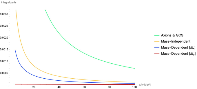
${\cal A}[Z^{\prime},Z]$    

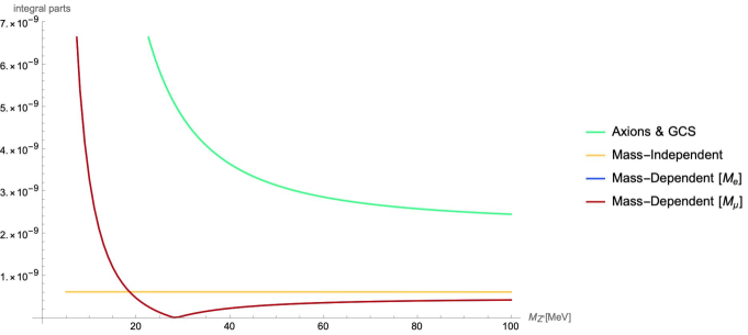
${\cal A}[Z^{\prime},Z^{\prime}]$    

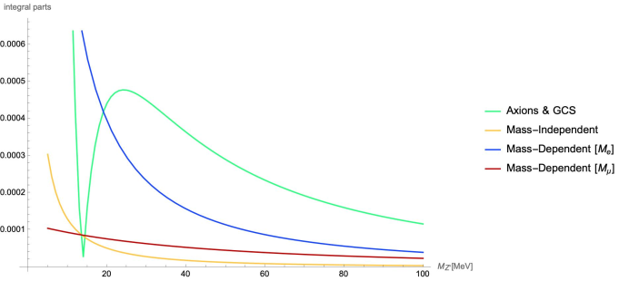
Figure 6: In these plot we compare the absolute value of the contribution coming from the amplitudes ${\cal A}[Z^{\prime},\gamma]$, ${\cal A}[Z^{\prime},Z]$, ${\cal A}[Z^{\prime},Z^{\prime}]$ excluding the anomalies $t_{ijk}$, the couplings $g_{i}$’s and charges $q^{f-A_{i}}$’s, and splitting them in the Axionic and GCS, the mass-independent and the mass-dependent contributions (for the fermion in the loop to be the electron or the muon $f=e/\mu$).

Finally, the $m_{f}$ dependant part of the triangle diagrams has a very long expression, which is omitted here. Even though we try to be generic in this stage of our analysis, we shall use some numerical results to compare each term’s contribution. In appendix D.1, we compare the contributions of each part (the axionic and GCS contribution, the mass-independent part contribution and the mass-dependent part) of the diagrams (• ‣ 4.3 - 4.117). We drop the charges and couplings and focus on the integrals in each case. These contributions depend on the mass of the $Z^{\prime}$. For reasons explained in the following section, we consider a low mass $Z^{\prime}$ model with $m_{Z^{\prime}}=5-100$ MeV, the mass of the muon $m_{\mu}$ and the mass of the $Z$, $m_{Z}$. In fig.6, we plot the absolute values of these contributions, and we conclude that the leading one is coming from the ${\cal A}[Z^{\prime},\gamma]$ and especially from the axionic and GCS parts.

5 A low mass $Z^{\prime}$ model and the $g-2$ of the muon

In this section, we apply our results to a low mass $Z^{\prime}$ model. We choose some values for the parameters of the model discussed in section 2 (a discussion of a toy-model and the chosen values is provided in the appendix A), and we evaluate the contribution of an anomalous $Z^{\prime}$ to the $g-2$ of the muon.

5.1 Justifying our choices

In the generic theory, the quarks are charged under the $Z^{\prime}$. In this case, the $Z^{\prime}$ can be abundantly produced in a hadron collider and the constraints on the $Z^{\prime}$ mass and coupling are rather stringent, its contribution to the $g-2$ is then relatively small. The situation becomes more interesting if we suppose that the anomalous $Z^{\prime}$ couples only to the lepton sector, i.e. leptophilic $Z^{\prime}$, Buras . In that case, we may classify $Z^{\prime}$ models into two categories, depending on whether $Z^{\prime}$ couples to the electron (a) or not (b).

1. In generic models of this category, the couplings to leptons can be independent. As there are strong constraints on the coupling to the electron, as mentioned above, in all such models the contributions to $g-2$ are also small. The only exception is to assume that the quantized charge of the electron is much smaller than that of the muon and tau, a highly unusual situation.

   A simple example of this class of models is a dark $U(1)$ gauge boson with a kinetic mixing. The kinetic mixing parameter $\epsilon$ may be defined such that the coupling of $Z^{\prime}$ to the electromagnetic current $J_{\rm em}^{\mu}$ is given by

   $${\cal L}_{\rm int} =-\epsilon eZ^{\prime}_{\mu}J_{\rm em}^{\mu}.$$ (5.130)

   The muon $g-2$ can be explained at one loop in this model with a parameter space $\epsilon\gtrsim 10^{-3}$ and $m_{Z^{\prime}}\lesssim 1$ GeV, which is however excluded by the search for a single $\gamma$ event in $e^{+}e^{-}\to\gamma Z^{\prime}$ followed by $Z^{\prime}\to$ invisible (such as neutrinos) at Babar BaBar:2017tiz . In particular, this channel constrains the $Z^{\prime}$ coupling to the electron as this is t-/u-channel process by exchanging electrons and emitting $Z^{\prime}$.

2. A typical example of this class of models contains a $Z^{\prime}$ that couples to $\mu$ (as well as $\tau$), but to no other fermions of the SM. The extra $U(1)$ symmetry is the gauged $U(1)_{L_{\mu}-L_{\tau}}$ symmetry. The experimental constraints are discussed in Jho:2019cxq (see also Kamada:2018zxi ), where the parameter space with $5~{}{\rm MeV}\lesssim m_{Z^{\prime}}\lesssim 200~{}{\rm MeV}$ and the gauge coupling $\sim 5\times 10^{-4}$ are compatible with this $Z^{\prime}$ giving a correction to the muon $g-2$ that has the right size to explain the discrepancy, as in (1.3).

It is important to note that in the anomalous $U(1)_{A}$ models, different flavors may, in principle, have different $U(1)_{A}$ charges as the anomaly cancellation required in most phenomenological models is not necessary. Therefore, for instance, the charges under the muon number $U(1)_{L_{\mu}}$ and the tau number $U(1)_{L_{\tau}}$ can be different, as opposed to the anomaly-free $U(1)_{L_{\mu}-L_{\tau}}$ model. We shall come back to this point later.

5.2 The one-loop contribution

We have evaluated the contribution of a leptonic $Z^{\prime}$ that couples only to the muon $\mu$ and tau $\tau$ fermions of the SM (class (b)). In this case, the lightest fermion that couples to $Z^{\prime}$ is the muon setting $f=\mu$.

We used the values

$$m_{\mu}=105~{}\textrm{MeV},~{}m_{Z}=91~{}\textrm{GeV},$$ (5.131)

$$g_{EM}q_{V}^{f-\gamma}=-e=-\sqrt{4\pi\alpha}=-0.30$$ (5.132)

$$g_{Z}q_{V}^{f-Z}={e-4e\sin^{2}\theta_{W}\over 4\sin\theta_{W}\cos\theta_{W}}=0.014,$$ (5.133)

$$g_{Z}q_{A}^{f-Z}=-{e\over 4\sin\theta_{W}\cos\theta_{W}}=-0.18,$$ (5.134)

where $\theta_{W}$ the Weinberg angle with $\sin^{2}\theta_{W}=0.23$, and $\alpha=1/137$ is the fine structure constant.

Assuming that the one-loop correction to the muon $g-2$ corresponds to the right magnitude (1.3), from (4.109) we may obtain the relation between $q_{V}^{\mu-Z^{\prime}}$, $q_{A}^{\mu-Z^{\prime}}$ and $m_{Z^{\prime}}$:

$$(g_{Z^{\prime}}q_{A}^{\mu-Z^{\prime}})^{2}\simeq{1\over{\cal F}_{A}[m^{2}_{\mu}/m^{2}_{Z^{\prime}}]}\left((g_{Z^{\prime}}q_{V}^{\mu-Z^{\prime}})^{2}{\cal F}_{V}[m^{2}_{\mu}/m^{2}_{Z^{\prime}}]-4\pi^{2}\frac{m_{Z^{\prime}}^{2}}{m_{\mu}^{2}}\delta a_{\mu}\right),$$ (5.135)

which means that for a given vectorial coupling, one can deduce the axial coupling necessary to fit the experimental constraint. We show in Fig.(1) the points in the plane ($q_{V}^{\mu-Z^{\prime}}$, $q_{A}^{\mu-Z^{\prime}}$) respecting the observed value $\delta a_{\mu}=2.5\times 10^{-9}$ for different values of $m_{Z^{\prime}}$ (1, 20 and 100 MeV).

For comparison, we also draw the corresponding line, which ensures a cancellation between the axial and vectorial charges ($\delta a_{\mu}=0$). The influence of the axial charge becomes stronger for small values of $q_{V}^{\mu-Z^{\prime}}$. For instance, for $m_{Z^{\prime}}=20$ MeV, we clearly see an asymptote around $g_{Z^{\prime}}q_{V}^{\mu-Z^{\prime}}=5.6\times 10^{-4}$ for $q_{A}^{\mu-Z^{\prime}}=0$, which value is in accordance with the result of Jho:2019cxq . On the other hand, as $q_{V}^{\mu-Z^{\prime}}$ increases, the value of $q_{A}^{\mu-Z^{\prime}}$ needed to respect, the $g-2$ measurement also increases due to its negative contribution, reaching $g_{Z^{\prime}}q_{A}^{\mu-Z^{\prime}}\simeq 5\times 10^{-5}$ for $g_{Z^{\prime}}q_{V}^{\mu-Z^{\prime}}\simeq 10^{-3}$.

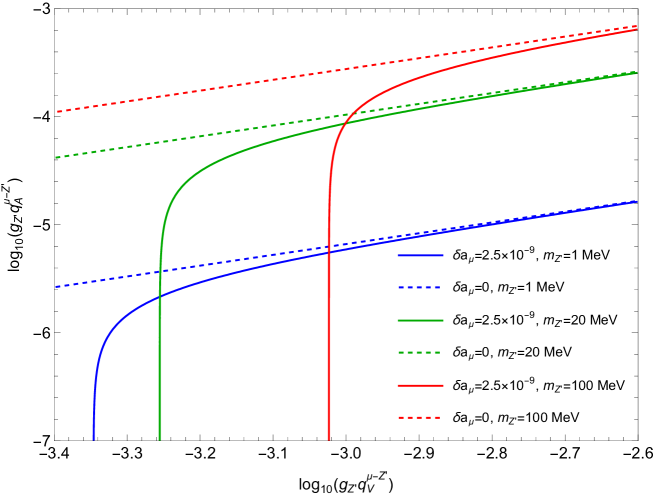
Figure 1: $g_{Z^{\prime}}q_{A}^{\mu-Z^{\prime}}$ as a function of $g_{Z^{\prime}}q_{V}^{\mu-Z^{\prime}}$, for fixed values of $\delta a_{\mu}$. Solid lines have fixed $\delta a_{\mu}=2.5\times 10^{-9}$ (1.3) and dashed lines have $\delta a_{\mu}=0$ for $m_{Z^{\prime}}=1,20,100$ MeV.

To understand the dependence of the $g-2$ on the vectorial and axial charges for light $Z^{\prime}$, it is easy to see that for $m_{Z^{\prime}}\ll m_{\mu}$, Eq.(5.135) reduces to

$$(g_{Z^{\prime}}q_{A}^{\mu-Z^{\prime}})^{2}\simeq\left(\frac{(g_{Z^{\prime}}q_{V}^{\mu-Z^{\prime}})^{2}}{8\pi^{2}}-\delta a_{\mu}\right)\times 4\pi^{2}\frac{m_{Z^{\prime}}^{2}}{m_{\mu}^{2}}.$$ (5.136)

This indicates that for $(g_{Z^{\prime}}q_{V}^{\mu-Z^{\prime}})^{2}\simeq 8\pi^{2}\delta a_{\mu}\simeq(5\times 10^{-4})^{2}$ (for the measured value $\delta a_{\mu}\simeq 3\times 10^{-9}$), $q_{A}^{\mu-Z^{\prime}}\simeq 0$. This is compatible with our numerical result obtained in Fig.(1).

The one-loop contribution can even vanish, i.e. $\delta a_{\mu}=0$, for $q_{V}^{\mu-Z^{\prime}}\simeq(\sqrt{2}m_{\mu}/m_{Z^{\prime}})q_{A}^{\mu-Z^{\prime}}\simeq 15\times q^{\mu-Z^{\prime}}_{A}$ for $m_{Z^{\prime}}=10$ MeV. In other words, for a 10 MeV $Z^{\prime}$, if $q_{V}^{\mu-Z^{\prime}}\simeq 15\times q_{A}^{\mu-Z^{\prime}}$, axial and vectorial contributions cancel, and higher-order effects, like those generated by the anomalies, should be considered.

This behavior of $g_{Z^{\prime}}q_{A}^{\mu-Z^{\prime}}$ is in accordance with Fig.(1), where we see that the $\delta a_{\mu}=0$ lines follow $\log(q_{A}^{\mu-Z^{\prime}})=\log(q_{V}^{\mu-Z^{\prime}})+$cst. The situation is different for heavier $Z^{\prime}$. In fact, one can observe from Eq.(4.110) that if $m_{Z^{\prime}}\gg m_{\mu}$, ${\cal F}_{V}\simeq\frac{1}{3}$, or the axial contribution needed to obtain the right $\delta a_{\mu}$ vanishes for

$$g_{Z^{\prime}}q_{V}^{\mu-Z^{\prime}}\simeq 6\times 10^{-4}\frac{m_{Z^{\prime}}}{m_{\mu}}\sqrt{\frac{\delta a_{\mu}}{3\times 10^{-9}}}.$$ (5.137)

An interesting feature is also that for a given pair ($q_{V}^{\mu-Z^{\prime}}$,$q_{A}^{\mu-Z^{\prime}}$), two values of $m_{Z^{\prime}}$ are allowed (the lines in Fig.(1) intersect). This comes from the features of Eq.(4.109), where the anomalous moment of the muon first increases with $m_{Z^{\prime}}$ for $m_{Z^{\prime}}\ll m_{\mu}$, whereas it decreases when $m_{Z^{\prime}}\gg m_{\mu}$. We illustrate this behavior on the upper panel of Fig.(2) where we plot $\delta a_{\mu}$ as function of $m_{Z^{\prime}}$ for different values of $q_{V}^{\mu-Z^{\prime}}$ and $g_{Z^{\prime}}q_{A}^{\mu-Z^{\prime}}=g_{Z^{\prime}}q_{V}^{\mu-Z^{\prime}}/10$, and the lower panel, the corresponding anomalous contribution of the $Z^{\prime}$. It is interesting to notice that the contribution of a $Z^{\prime}$ to $g-2$ reaches a maximum for a $Z^{\prime}$ mass of $\sim 40$ MeV, much below the electroweak scale. The $4.2\sigma$ discrepancy (1.3) can even be obtained for $m_{Z^{\prime}}=40$ MeV and $g_{Z^{\prime}}(q_{V}^{\mu-Z^{\prime}},q_{A}^{\mu-Z^{\prime}})$ = ($0.81\times 10^{-3}$, $0.81\times 10^{-4}$).

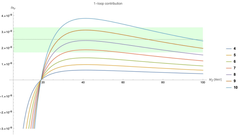
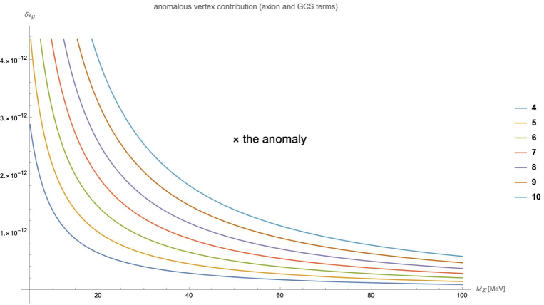
Figure 2: The two plots give the contribution to the $g-2$ from the one-loop and the two-loop (anomalous) amplitudes, for different $g_{Z^{\prime}}q_{V}^{\mu-Z^{\prime}}=10\times g_{Z^{\prime}}q_{A}^{\mu-Z^{\prime}}=(4-10)\times 10^{-4}$, represented by different colored lines. In the first plot, the dashed line is the $\delta a$ (1.3) and the green zone the $1\sigma$ uncertainty ($\delta\sigma=\sqrt{63^{2}+43^{2}}\times 10^{-11}$). Notice that the contribution from $Z^{\prime}$ with masses below the 20 MeV becomes negative. In the second diagram, we present the contribution of the anomalous diagram without the overall anomalous factor $t_{ijk}$. For an anomaly equal to 100, this contribution is within the experimental error and for even larger anomaly values becomes dominant.

For the specific choice of parameters, $g_{Z^{\prime}}q_{V}^{\mu-Z^{\prime}}=10\times g_{Z^{\prime}}q_{A}^{\mu-Z^{\prime}}=(4-10)\times 10^{-4}$, the axial and vectorial contributions arise with an opposite sign, there exists a region of the parameter space $m_{Z^{\prime}}\simeq 20$ MeV, where both contributions cancel exactly, rendering the contribution generated by the anomalies (4.118) dominant (fig 2, upper plot). The values of the couplings fitting $\delta a_{\mu}$ are of the order of $\sim 10^{-4}$ and do not enter into conflict with other $Z^{\prime}$ searches such as the neutrino trident production, which rules out the coupling greater than $10^{-3}$ for $m_{Z^{\prime}}\lesssim{\cal O}(10)$ MeV Altmannshofer:2014pba .

5.3 The anomaly contribution

As we have already mentioned, we have three different sets of diagrams depending on the type of the bosons $A$ and $B$ in (4.112). These diagrams can be grouped as

• ${\cal A}[Z^{\prime},\gamma]$ given in (• ‣ 4.3)

• ${\cal A}[Z^{\prime},Z]$ given in (• ‣ 4.3)

• ${\cal A}[Z^{\prime},Z^{\prime}]$ given in (• ‣ 4.3)

• ${\cal A}[Z,\gamma]$ given in (• ‣ 4.3)

• ${\cal A}[Z,Z]$ given in (4.117)

Each of these sets of diagrams can be split in

• the axionic $\&$ GCS contribution,

• the $m_{f}$ independent part of the triangle diagram and

• the $m_{f}$ dependent part.

According to (2.64), the typical cutoff of our model is $\Lambda\sim 40$ TeV, where we took, $m_{Z^{\prime}}\simeq 20$ MeV, $g_{A}\simeq 10^{-4}$ and $t_{ijk}\simeq 100$. This is 1-2 orders of magnitude above the experimental scales. In retrospect, it implies that in such a case there is new physics (new massive charged fermions) within the reach of the next generation of experiments.

Next, we make comparisons between the five different diagrams and the three different contributions per diagram in order to find the leading one.

We start by comparing the contributions from the a, b and c parts in each diagram separately. We drop the overall factor that contains the charges and the couplings, and we focus on the integrals. These formulae depend only on the masses of the fields involved. We present our results in appendix D. In all cases, the leading contribution per diagram comes from the axionic and GCS vertices.

Next, comparing the full diagrams (with the couplings and charges) (• ‣ 4.3 - 4.117) we find that the leading contribution to the $g-2$ is coming from ${\cal A}[Z^{\prime},\gamma]$ diagram, with one photon and an anomalous $Z^{\prime}$ in the loop. The rest are suppressed by extra massive gauge fields in the loop (the photon is replaced by $Z$ or $Z^{\prime}$). Additionally, the contribution of the ${\cal A}[Z,\gamma]$, ${\cal A}[Z,Z]$ are suppressed by the mass of the $Z$, which is the heaviest boson in our analysis.

The leading anomalous contribution

According to our previous discussion, we focus on the leading contribution coming from the diagram ${\cal A}[Z^{\prime},\gamma]$ and especially the axion & GCS vertex in the loop. This contribution depends on four parameters. The mass of the $Z^{\prime}$, $m_{Z^{\prime}}$, the vectorial/axial couplings of the $Z^{\prime}$ to the muon $q_{V/A}^{\mu-Z^{\prime}}$ and the anomaly trace $t_{Z^{\prime}\gamma\gamma}$. To illustrate our results, we shall scan our parameter space $m_{Z^{\prime}}\in(5-100)$ MeV with $g_{Z^{\prime}}q_{V}^{\mu-Z^{\prime}}=10\times g_{Z^{\prime}}q_{A}^{\mu-Z^{\prime}}=(4-10)\times 10^{-4}$.

The overall anomaly $t_{ijk}$ is a free parameter that can take any positive or negative value, depending on the number of fermions charged under the relevant gauge bosons. If we assume that the charges of the fermions under the anomalous $A^{\mu}$ are big (bigger than 4), the anomaly $t_{ijk}$ can be huge.

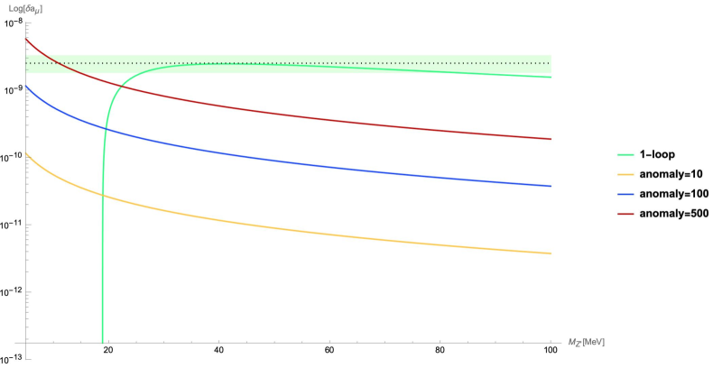
Figure 3: In this plot, we present the one-loop contribution of an anomalous $Z^{\prime}$ to the $g-2$ of the muon for masses $m_{Z^{\prime}}=5-100$ MeV and fixed couplings $g_{Z^{\prime}}q_{V}^{\mu-Z^{\prime}}=10\times g_{Z^{\prime}}q_{A}^{\mu-Z^{\prime}}=8\times 10^{-4}$. We also provide the contribution from the anomalous coupling for an anomaly $t_{ijk}=10,100,500$.

Alternatively, $t_{ijk}$ could take huge values if the coupling-full charges $q^{f-Z^{\prime}}_{V/A}$ of a fermion $f$ is many orders of magnitude larger than $q^{\mu-Z^{\prime}}_{V/A}$. Notice for example, that the coupling between $Z^{\prime}$ and $\tau$ is the least constrained interaction in experiments if $Z^{\prime}$ is purely leptonic force, which allows us to take $q^{\tau-Z^{\prime}}_{V/A}$ up to ${\cal O}(1)$.

In fig 2 we present two plots. The upper plot gives the one-loop contribution for different values of $g_{Z^{\prime}}q_{V}^{\mu-Z^{\prime}}=10\times g_{Z^{\prime}}q_{A}^{\mu-Z^{\prime}}=(4-10)\times 10^{-4}$. The upper plot shows the contribution of the anomalous diagrams without the overall anomaly $t_{ijk}$ for similar values of $g_{Z^{\prime}}q_{V}^{\mu-Z^{\prime}}$, $g_{Z^{\prime}}q_{A}^{\mu-Z^{\prime}}$. For large values of the anomaly, the contribution of the anomalous diagram becomes leading and can absorb the full experimental discrepancy (1.3). As an example, we fix the values $g_{Z^{\prime}}q_{V}^{\mu-Z^{\prime}}=10\times g_{Z^{\prime}}q_{A}^{\mu-Z^{\prime}}=8\times 10^{-4}$ and we compare the one-loop contribution with the anomalous contribution for values of the anomalous trace $t_{ijk}=10,100,500$ in fig 3, and in fig 4 we add the one-loop and the anomalous contributions for the above values of the anomaly.

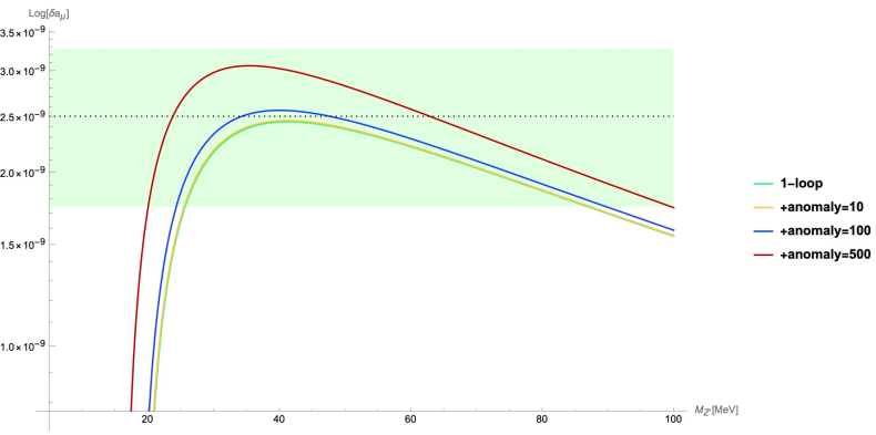
Figure 4: In this plot, we add the one-loop and the anomalous contributions to the $g-2$ of the muon for masses $m_{Z^{\prime}}=5-100$ MeV and fixed couplings $g_{Z^{\prime}}q_{V}^{\mu-Z^{\prime}}=10\times g_{Z^{\prime}}q_{A}^{\mu-Z^{\prime}}=8\times 10^{-4}$. We use for the anomaly $t_{ijk}=10,100,500$.

It is very interesting to note that for $m_{Z^{\prime}}\sim 20$ MeV and $g_{Z^{\prime}}q_{V}^{\mu-Z^{\prime}}=10\times g_{Z^{\prime}}q_{A}^{\mu-Z^{\prime}}$ the one-loop contribution becomes very small due to the competing vectorial and axial coupling, and higher loop non-anomalous effects cannot contribute enough. However, if the $Z^{\prime}$ is anomalous, with a large anomaly, the axionic and GCS terms take the lead, and they can reproduce the full discrepancy (1.3).

As a final but important remark, we stress that the anomaly contribution is an effect that also reflects the UV properties of the theory. Although its contribution to $g-2$ is of two-loop order, it is of a different nature than the other two-loop contributions. In particular, if the standard two-loop contribution is comparable to the one-loop contribution, this signals the breakdown of perturbation theory. If the anomalous contribution is comparable to the one-loop contribution, this is not a signal of the breakdown of perturbation theory, as the anomaly is one loop only.

6 Leptophilic $Z^{\prime}$ in D-brane realizations of the SM

In this section, we shall discuss to what extent string theory models are possible where the $Z^{\prime}$ couples only to leptons and, most importantly, to $\mu$ and $\tau$ but not the electron.

Anomalous $U(1)$’s are common in D-brane realizations of the SM, Kiritsis:2003mc ; rev1 ; rev2 and are the generic low-energy states with non-zero masses in perturbative string theory, as their masses are one-loop effects, AK . In this section, we discuss the possibility that the extension of the SM with one or more anomalous U(1)’s that couple to leptons (and specifically to the muon and tau and not to the electron) with a coupling of the order of $10^{-4}$, can be realized in semi-realistic D-brane configurations.

In this framework, SM particles are fluctuations of a “local set of D-branes”. “Local” means a set of branes wrapping various cycles of the internal compact six-dimensional manifold and intersecting in an area in transverse space whose linear size is of the order of or smaller than the string length. The SM particles, in this context, are realized by the lightest fluctuations of open strings stretched between the local stack of D-branes, AKT ; AIQU ; AKRT ; AD ; ADKS ; Anastasopoulos:2009mr ; Anchordoqui:2021lmm ; Anchordoqui:2022kuw . This, as a result, realizes the Standard model spectrum in terms of only bi-fundamental representations of the local D-brane gauge group. In particular, the general rules can be summarised as follows:

• strings with both ends on a stack of $N$ parallel D-branes transform in the adjoin of $U(N)$ which splits in $SU(N)\times U(1)_{N}$ and

• strings stretched from a stack of $N$ to a stack of $M$ D-branes transform under $(N,+1;\bar{M},-1)$, where $\pm 1$ are the charges under the abelian parts.

The SM’s $SU(3)\times SU(2)\times Y$ is typically described by a stack of three, two, and some single D-branes. Next, we would like to analyze different cases according to the number of stacks where the SM strings/particles are located:

• Three stack models AD .

  If the SM particles are described by strings stretched between three different stacks of D-branes AD , there is no linear combination between these three abelian factors that describes the lepton number. Therefore, a model which contains a leptophilic $Z^{\prime}$ cannot be realized with three D-brane stacks.

• Four stack models ADKS .

  In four stack models, the hypercharge and the Lepton number can be realized as a linear combination of the four abelian factors coming from each stack. The different hypercharge and lepton number embeddings are given in ADKS . However, in all these cases, the hypercharge and the Lepton numbers are not orthogonal, allowing for large kinetic mixing and questioning the viability of such a model at the phenomenological level.

  We also searched cases where an “approximate” Lepton number, orthogonal to the hypercharge, is realized, where leptons have almost $\pm 1$ changes and the rest of the SM particles are almost zero. However, no such case was found.

• Five stack models or more.

  In this case, configurations where the hypercharge is a linear combination of four U(1)’s, and a universal Lepton number is coming from the fifth D-brane are possible Antoniadis:2021mqz . Here, $Y$ and $L$ are orthogonal by construction. A sixth D-brane is required to have a non-universal Lepton number where the muon and tau are charged, and the electron is not. The muon and tau are strings with one endpoint on the fifth D-brane (where the Lepton number lives), and the electron is a string with one endpoint on the sixth D-brane. The leptophilic U(1) coupling can take values of the order of $10^{-4}$ depending on the volumes that this D-brane wraps.

7 Conclusions

In this work, we have computed several contributions from an extra anomalous gauge boson $Z^{\prime}$ to the $g-2$ of the muon. We supplemented the one-loop contribution with additional contributions that are due to anomalous couplings of the Chern-Simons type. These higher-order contributions are unavoidable if the SM spectrum is anomalous concerning the U(1) of the $Z^{\prime}$. Such (gauge) anomalies are cancelled by the effective generalized CS terms. In the UV theory, the anomalies are cancelled by extra groups of fermions with masses well above the UV cutoff of the EFT. Integrating out these anomaly cancelling fermions induces the anomaly cancelling generalized CS terms in the EFT. We have shown that the anomalous contributions to $g-2$ are of two-loop order and therefore generically subleading to the one-loop (non-anomalous) contributions. In this generic case, once a $Z^{\prime}$ is discovered, measuring the subleading contributions provides a window into the anomalous massive spectrum of the theory.

However, depending on the $Z^{\prime}$ charges of leptons, the one-loop contribution may be unnaturally small due to cancellations. In such a case, the anomalous contributions may become comparable or dominant to the one-loop ones. This does not signal the breakdown of perturbation theory as the anomalous vertex is one loop only and does not obtain higher loop corrections. In this second case, the $g-2$ excess could be explained in the region of parameter spaces $m_{Z^{\prime}}\simeq 40$ MeV, and charges of the muon to the $Z^{\prime}$, $g_{Z^{\prime}}(q_{V}^{\mu-Z^{\prime}},q_{A}^{\mu-Z^{\prime}})\simeq(10^{-3},10^{-4})$. The axial and vectorial contributions arise with negative relative signs, and there are regions of the parameter space where the anomalous higher-order contributions do dominate. If the overall anomaly traces are large, the anomalous contribution is leading, and it can even reproduce the whole discrepancy (1.3). We also note that in such cases the cutoff of the theory is low enough and this implies that new charged fermions are within the reach of future colliders.

APPENDIX

Appendix A A UV completion of the effective model

In this appendix, we present a UV completion of the effective model presented in section 2.

We consider an anomaly-free model with the SM fermions (massless) and several extra massless fermions $\chi_{i}$. We also have two Higgs fields, $H$ the doublet Higgs field of the SM and a extra scalar field $S$.

• The SM fermions $\psi_{SM,i}$ and Higgs $H$ are generically charged under $U(1)_{A}$ beyond the charges they gave under the SM gauge group.

• The extra fermions $\chi_{i}$ are charged under the $U(1)_{Y}\times U(1)_{A}\times SU(2)_{W}$ .

• The extra scalar $S$ is charged only under $U(1)_{A}$, and it has Yukawa couplings only with the extra fermions $\chi_{i}$.

The action schematically is

$${\cal L}={\cal L}_{SM}-{1\over 4}F^{2}_{A}+\bar{\chi}_{i}\gamma_{\mu}D^{\mu}\chi_{i}+|DS|^{2}+\lambda_{S}(|S|^{2}-V^{2})^{2}+Y_{ij}\bar{\chi}_{i}\chi_{j}S+c.c.$$ (A.138)

where ${\cal L}_{SM}$ is the action of the SM augmented by the minimal couplings of the SM fields to $U(1)_{A}$.

Anomaly conditions require that the contribution to the anomalies from all triangle diagrams (SM plus the extra fermions) cancel out.

We assume that $V\gg v_{H}$, where $v_{H}$ is the SM HIggs vev, and there is very small mixing between $H$ and $S$.

• Upon $S$-induced symmetry breaking, the additional U(1)_A gauge field ($A^{\mu}$) becomes massive with mass $M=g_{A}q^{S-A}V$, where $q^{S-A}$ is the charge of $S$ under $A^{\mu}$.

• $S$ becomes massive with $m_{S}=\sqrt{2\lambda_{S}}V$.

• The fermions $\chi_{i}$ become massive, forming in pairs Dirac fermions, with masses $Y_{ij}V$, where $Y_{ij}$ are the Yukawa couplings in (A.138).

We assume that the S-mass as well as the extra fermion masses are much larger than the mass $M$ of $A_{\mu}$

$$M\ll\Lambda_{S,\chi}\equiv min\{\sqrt{2\lambda_{S}}V,Y_{ij}V\}$$ (A.139)

and we integrate out the $S$ field as well as the extra massive fermions $\chi_{i}$. This defines our effective field theory. It contains the Standard model fields, the $U(1)_{A}$ gauge boson , and the phase of $S$ that appears as a low-energy axion field. (see a schematic representation of our toy-model in fig. 5).

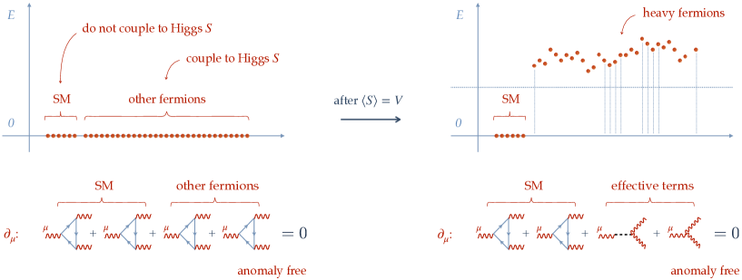
Figure 5: A schematic representation of the toy-model.

The theory described above is rather general. In many cases, the subset of fermion $\chi_{i}$ that become heavy and are integrated out, may have non-zero anomaly contributions to the symmetries of the effective field theory, ABDK .These contributions must be visible in the effective theory and indeed they appear from the axionic, and GCS effective terms ABDK ; PA ; Anastasopoulos:2008jt .

A.1 Obtaining a low mass $Z^{\prime}$ (toy) model

As mentioned above, some of the parameters of our fundamental theory are

• the large vev of the Higgs field $S$ which we denote by $\langle S\rangle=V$,

• the parameter $\lambda_{S}$ which also controls the mass $m_{S}=\sqrt{2\lambda_{S}}V$ of the heavy scalar $S$,

• the Yukawa couplings $Y_{ij}$ responsible for giving heavy masses to all extra fermions $\chi_{i}$, and

• the mass of $A^{\mu}$, $m_{A}=g_{A}q^{S-A}V$.

Next, we assign some values to the parameters above.

We assume that the Yukawa couplings $Y_{ij}$ and the coupling $\lambda_{S}$ are in the perturbation regime, $Y_{ij},\lambda_{S}\sim 10^{-1}$. For the masses of the heavy fermions and the extra scalar to be above the 40 TeV, we obtain a value

$$V\sim 400\textrm{TeV}~{}~{}~{}~{}\to~{}~{}~{}~{}m_{\textrm{heavy fermions}},m_{S}\sim 40\textrm{TeV}$$ (A.140)

With this value of the vev of $S$, and a coupling $g_{Z^{\prime}}\sim 10^{-4}$, we obtain

$$g_{Z^{\prime}}q^{S-Z^{\prime}}V\sim 10-100\textrm{MeV}~{}~{}~{}~{}\to~{}~{}~{}~{}q^{S-Z^{\prime}}\sim 2.5\times 10^{-3}-2.5\times 10^{-2}$$ (A.141)

where $q^{S-Z^{\prime}}$ is the charge of the scalar $S$ under the $A_{\mu}$ vector field.

Finally, we would like to make some comments about the value of the tree-level anomaly of the effective theory. In our effective theory, among the anomaly-related contributions to $g-2$ , the dominant one is originating from ${\cal A}[Z^{\prime},\gamma]$ (• ‣ 4.3). This contributions is proportional to the anomaly trace $t_{Z^{\prime}\gamma\gamma}$. Since we assume in the main text that the only SM fermions charged under the anomalous $Z^{\prime}$ are the muon and tau leptons, we can evaluate

$$t_{Z^{\prime}\gamma\gamma}=\sum_{f=\mu,\tau}q_{A}^{f-Z^{\prime}}q_{V}^{f-\gamma}q_{V}^{f-\gamma}=q_{A}^{\mu-Z^{\prime}}+q_{A}^{\tau-Z^{\prime}}$$ (A.142)

since $q_{A}^{f-\gamma}=0$ for all SM fermions and $q_{V}^{\mu/\tau-\gamma}=-1$. Assuming also that $q_{A}^{\tau-Z^{\prime}}\gg q_{A}^{\mu-Z^{\prime}}$, the axial charge of the tau lepton controls the anomaly. Finally, imposing the unitarity bound $g_{Z^{\prime}}q^{\tau-Z^{\prime}}<{\cal O}(1)$, and $g_{Z^{\prime}}\sim 10^{-4}$, we obtain

$$t_{Z^{\prime}\gamma\gamma}\sim q_{A}^{\tau-Z^{\prime}}<10^{4}\;.$$ (A.143)

This allows for large anomaly values, that control the anomalous contribution of the $g-2$ of the muon. In the main part of the paper, we shall explore the range

$$50<t_{Z^{\prime}\gamma\gamma}<500$$ (A.144)

Appendix B Feynman rules

These are the Feynman rules needed for our computation:

• Propagators (unitary gauge)

  $$\gamma~{}~{}~{}:~{}~{}~{}~{}~{}~{}~{}~{}D_{\gamma}^{\mu\nu}(k)={-ig^{\mu\nu}\over k^{2}}$$ (B.145)

  $$Z/Z^{\prime}~{}:~{}~{}~{}~{}~{}~{}~{}D_{\tilde{A}}^{\mu\nu}(k)={i\over k^{2}-m_{\tilde{A}}^{2}}\left(g^{\mu\nu}-{k^{\mu}k^{\nu}\over m_{\tilde{A}}^{2}}\right)$$ (B.146)

  The fermions and bosons (Higgs) in the broken phase have propagators

  $$\textrm{scalar}~{}:~{}~{}~{}~{}~{}~{}\Delta(p)={i\over p^{2}-m^{2}_{s}}$$ (B.147)

  $$\textrm{lepton}~{}:~{}~{}~{}~{}~{}S(p)={i\over\raise 0.6458pt\hbox{$/$}\kern-5.70007ptp-m_{l}}$$ (B.148)

• Minimal couplings

  $$\begin{array}[]{llllllllll}\textrm{lepton $\ell$ with photon}&&\to&&-ig_{EM}q^{\ell-\gamma}_{V}\gamma_{\mu}\\ \textrm{lepton $\ell$ with $Z$}&&\to&&-ig_{Z}q^{\ell-Z}\gamma_{\mu}=-ig_{Z}\left(q^{\ell-Z}_{V}\mathbb{I}-q^{\ell-Z}_{A}\gamma_{5}\right)\gamma_{\mu}\\ \textrm{lepton $\ell$ with $Z^{\prime}$}&&\to&&-ig_{Z^{\prime}}q^{\ell-Z^{\prime}}\gamma_{\mu}=-ig_{Z^{\prime}}\left(q^{\ell-Z^{\prime}}_{V}\mathbb{I}-q^{\ell-Z^{\prime}}_{A}\gamma_{5}\right)\gamma_{\mu}\end{array}$$ (B.152)

  where $g_{EM}$, $g_{Z}=g_{2}/2\cos\theta_{W}$, $g_{Z^{\prime}}$ the coupling constants of the electromagnetism the $Z$ and the $Z^{\prime}$ (see (B.153)).

B.1 SM leptons and gauge fields in the broken (photon) basis

Applying the rotation matrix $O$ to the SM part of (2.28) and we collect the couplings between leptons and gauge bosons (in the broken phase)

$${\cal L}_{leptons} = e\bar{e}_{i}\gamma_{\mu}e_{i}A^{\mu}_{\gamma}-{g_{2}\over 2\sqrt{2}}W^{+}_{\mu}\bar{e}_{j}\gamma^{\mu}(1-\gamma_{5})\nu_{i}{\cal U}^{\nu}_{ji}-{g_{2}\over 2\sqrt{2}}W^{-}_{\mu}\bar{\nu}_{j}\gamma^{\mu}(1-\gamma_{5})e_{i}{\cal U}^{\nu\dagger}_{ji}$$ (B.153)

$$-{g_{2}\over 2\cos\theta_{W}}Z_{\mu}\bar{e}_{i}(q_{V}^{e-Z}\gamma^{\mu}-q_{A}^{e-Z}\gamma^{\mu}\gamma_{5})e_{i}-{g_{2}\over 2\cos\theta_{W}}Z_{\mu}\bar{\nu}_{i}(q_{V}^{\nu-Z}\gamma^{\mu}-q_{A}^{\nu-Z}\gamma^{\mu}\gamma_{5})\nu_{i}$$

$$-g_{Z^{\prime}}Z^{\prime}_{\mu}\bar{e}_{i}(q_{V}^{e-Z^{\prime}}\gamma^{\mu}-q_{A}^{e-Z^{\prime}}\gamma^{\mu}\gamma_{5})e_{i}-g_{Z^{\prime}}Z^{\prime}_{\mu}\bar{\nu}_{i}(q_{V}^{\nu-Z^{\prime}}\gamma^{\mu}-q_{A}^{\nu-Z^{\prime}}\gamma^{\mu}\gamma_{5})\nu_{i}$$

where $ij=1,2,3$ for the different families of the SM and ${\cal U}^{\nu}_{ji}$ the mixing matrix of the leptons.

Appendix C The anomalous coupling

As we have already mentioned, the anomalous coupling splits into two parts

$$\Gamma_{\mu\nu\rho}^{ijk}|_{\textrm{total}} = \Gamma_{\mu\nu\rho}^{ijk}|_{\textrm{one-loop}}+\Gamma_{\mu\nu\rho}^{ijk}|_{\textrm{axion}}+\Gamma_{\mu\nu\rho}^{ijk}|_{\textrm{GCS}}$$

$$= \Big{(}\Gamma_{\mu\nu\rho}^{ijk}|^{\textrm{C=even}}_{\textrm{one-loop}}\Big{)}+\Big{(}\Gamma_{\mu\nu\rho}^{ijk}|^{\textrm{C=odd}}_{\textrm{one-loop}}+\Gamma_{\mu\nu\rho}^{ijk}|_{\textrm{axion}}+\Gamma_{\mu\nu\rho}^{ijk}|_{\textrm{GCS}}\Big{)}$$

where the C even part identically vanishes due to Furry’s theorem. Therefore, in diagrams

$$+\scalebox{0.7}{ \leavevmode\hbox to0pt{\vbox to0pt{\text{[drawing]}}}}+\scalebox{0.7}{ \leavevmode\hbox to0pt{\vbox to0pt{\text{[drawing]}}}}+... A_{i}^{\mu} A_{k}^{\rho} A_{j}^{\nu} k_{3} a k_{2} k_{1} A_{i}^{\mu} A_{k}^{\rho} A_{j}^{\nu} k_{3} k_{2} k_{1} A_{i}^{\mu} A_{k}^{\rho} A_{j}^{\nu} k_{3} a k_{2} k_{1} A_{i}^{\mu} A_{k}^{\rho} A_{j}^{\nu} k_{3} k_{2} k_{1}$$

where the ellipsis indicates that we should take all permutations of the axionic propagator with all other legs. The parametrization has been analytically evaluated in ABDK , and here we present the results

$$\Gamma^{ijk}_{\mu\nu\rho}|_{\textrm{one-loop}}^{\textrm{CP=odd}}=g_{i}g_{j}g_{k}t^{ijk}\Big{(}\varepsilon_{\mu\nu\rho\sigma}(A_{1}k_{2}^{\sigma}+A_{2}k_{1}^{\sigma})$$ (C.156)

$$~{}~{}~{}~{}~{}~{}~{}~{}~{}~{}~{}~{}~{}~{}~{}~{}~{}~{}~{}~{}~{}~{}~{}+(B_{1}k_{2\nu}+B_{2}k_{1\nu})\varepsilon_{\mu\rho\sigma\tau}k_{2}^{\sigma}k_{1}^{\tau}+(B_{3}k_{2\rho}+B_{4}k_{1\rho})\varepsilon_{\mu\nu\sigma\tau}k_{2}^{\sigma}k_{1}^{\tau}\Big{)}$$

$$\Gamma^{ijk}_{\mu\nu\rho}|_{\textrm{axion}}=-g_{i}g_{j}g_{k}\Big{(}M^{i}_{I}C^{jk}_{I}{k_{3\mu}\over k_{3}^{2}}\varepsilon_{\nu\rho\sigma\tau}k_{2}^{\sigma}k_{1}^{\tau}$$

$$~{}~{}~{}~{}~{}~{}~{}~{}~{}~{}~{}~{}~{}~{}~{}~{}~{}~{}~{}~{}~{}~{}~{}~{}~{}~{}~{}~{}+M^{j}_{I}C^{ki}_{I}{k_{1\nu}\over k_{1}^{2}}\varepsilon_{\rho\mu\tau\sigma}k_{2}^{\sigma}k_{3}^{\tau}+M^{k}_{I}C^{ij}_{I}{k_{2\rho}\over k_{2}^{2}}\varepsilon_{\mu\nu\tau\sigma}k_{3}^{\sigma}k_{1}^{\tau}\Big{)}~{}~{}~{}~{}~{}~{}~{}~{}$$ (C.157)

$$\Gamma^{ijk}_{\mu\nu\rho}|_{\textrm{GCS}}=-g_{i}g_{j}g_{k}\Big{(}E^{ij,k}\varepsilon_{\mu\nu\rho\sigma}k_{2}^{\sigma}+E^{jk,i}\varepsilon_{\nu\rho\mu\sigma}k_{3}^{\sigma}+E^{ki,j}\varepsilon_{\rho\mu\nu\sigma}k_{1}^{\sigma}\Big{)}$$ (C.158)

where the anomaly coefficient $t^{ijk}$ contains the trace anomaly and $g_{i/j/k}$ the minimal couplings between the fermions in the loop and the gauge fields $A^{\mu}_{i/j/k}$. The $B_{1},B_{2},B_{3},B_{4}$ are finite coefficients (functions of $k_{1},k_{2}$)

$$B_{1}(k_{1},k_{2})=-B_{4}(k_{2},k_{1})=-{i\over 8\pi^{2}}\int^{1}_{0}d\alpha\int^{1-\alpha}_{0}d\beta{2\alpha\beta\over\alpha k^{2}_{2}+\beta k^{2}_{1}-(\alpha k_{2}-\beta k_{1})^{2}-{m_{f}^{2}}}~{}~{}~{}~{}~{}~{}~{}~{}~{}$$ (C.159)

$$B_{2}(k_{1},k_{2})=-B_{3}(k_{2},k_{1})=-{i\over 8\pi^{2}}\int^{1}_{0}d\alpha\int^{1-\alpha}_{0}d\beta{2\beta(1-\beta)\over\alpha k^{2}_{2}+\beta k^{2}_{1}-(\alpha k_{2}-\beta k_{1})^{2}-{m_{f}^{2}}}~{}~{}~{}~{}~{}~{}$$ (C.160)

Note that the above coefficients (in particular (C.160)) contain an IR divergence in the massless $m_{f}\to 0$ limit.

We should mention that the (scheme-dependant) coefficients $A_{1},A_{2}$ can be eliminated in terms of the finite and unambiguous coefficients $B_{i}$’s, by using Bose symmetry and $C_{A}$ the standard anomaly coefficient ABDK .

$$A_{1}=-{C_{A}\over 3}-k_{1}\cdot k_{2}B_{1}-k_{1}^{2}B_{2}$$ (C.161)

$$A_{2}=+{C_{A}\over 3}-k_{2}^{2}B_{3}-k_{1}\cdot k_{2}B_{4}$$ (C.162)

$$A_{1}-A_{2}={C_{A}\over 3}$$ (C.163)

Requiring that the Ward identities be satisfied, we obtain the anomaly conditions for the most generic case to be ABDK

$$\left.\begin{array}[]{lllll}&k_{1}^{\nu}\Gamma^{ijk}_{\mu\nu\rho}|_{\textrm{total}}=0\\ &k_{2}^{\rho}\Gamma^{ijk}_{\mu\nu\rho}|_{\textrm{total}}=0\\ &k_{3}^{\mu}\Gamma^{ijk}_{\mu\nu\rho}|_{\textrm{total}}=0\end{array}\right\}~{}~{}\to~{}~{}\begin{array}[]{rlllll}&C_{A}~{}t_{ijk}&=&M_{I}^{k}C^{ij}_{I}+M_{I}^{j}C^{ki}_{I}+M_{I}^{i}C^{jk}_{I}\\ &3E^{ij,k}&=&M_{I}^{i}C^{jk}_{I}-M_{I}^{j}C^{ki}_{I}\\ &3E^{jk,i}&=&M_{I}^{j}C^{ki}_{I}-M_{I}^{k}C^{ij}_{I}\\ &3E^{ki,j}&=&M_{I}^{k}C^{ij}_{I}-M_{I}^{i}C^{jk}_{I}\end{array}$$ (C.171)

where summation over $I$ is understood. In these conditions, we have considered the coefficients’ structure. Therefore, the symmetric combination of the $M_{I}^{(i}C_{I}^{jk)}$ cancels the democratically distributed anomaly, and the antisymmetric part $M_{I}^{[i}C_{I}^{j]k}$ cancels the GCS terms.

The anomalous coupling in our case

In this section, we use the anomalous conditions found in (2.35) to give the form of the different couplings (we use that $k_{3}=-k_{1}-k_{2}$)

• The $AYY$ anomalous coupling

  Using the anomaly conditions (2.35) we obtain the anomaly relations

  $$E_{AY,Y}={C_{A}}t_{AYY}~{},~{}~{}~{}~{}MC_{YY}=-2C_{A}t_{AYY}$$ (C.172)

  and inserting them in (C.156), (C.157), (C.158) and using (C.159), (C.160), we obtain the contributions from the triangle, the axionic and GCS terms as

  $$\Gamma^{AYY}_{\mu\nu\rho}|_{\textrm{one-loop}}^{\textrm{CP=odd}}=\Gamma^{AYY}_{\mu\nu\rho}|_{\textrm{one-loop}}^{\textrm{mass-independent}}+\Gamma^{AYY}_{\mu\nu\rho}|_{\textrm{one-loop}}^{\textrm{mass-dependent}}$$ (C.173)

  $$\Gamma^{AYY}_{\mu\nu\rho}|_{\textrm{one-loop}}^{\textrm{mass-independent}}=-g_{A}g_{Y}^{2}t_{AYY}{C_{A}\over 3}\varepsilon_{\mu\nu\rho\sigma}(k_{2}^{\sigma}-k_{1}^{\sigma})$$ (C.174)

  $$\Gamma^{AYY}_{\mu\nu\rho}|_{\textrm{one-loop}}^{\textrm{mass-dependent}}=g_{A}g_{Y}^{2}\sum_{f}q^{f-A}q^{f-Y}q^{f-Y}\Big{(}-\Big{(}k_{1}\cdot k_{2}B_{1}^{f}+k_{1}^{2}B^{f}_{2}\Big{)}\varepsilon_{\mu\nu\rho\sigma}k_{2}^{\sigma}$$

  $$~{}~{}~{}~{}~{}~{}~{}~{}~{}~{}~{}~{}~{}~{}~{}~{}~{}~{}~{}~{}~{}~{}~{}~{}~{}~{}~{}~{}~{}~{}~{}~{}~{}~{}~{}~{}~{}~{}~{}~{}~{}~{}~{}~{}~{}~{}~{}~{}~{}~{}~{}~{}-\Big{(}k_{2}^{2}B^{f}_{3}+k_{1}\cdot k_{2}B^{f}_{4}\Big{)}\varepsilon_{\mu\nu\rho\sigma}k_{1}^{\sigma}~{}~{}~{}~{}~{}~{}$$

  $$~{}~{}~{}~{}~{}~{}~{}~{}~{}~{}~{}~{}~{}~{}~{}~{}~{}~{}~{}~{}~{}~{}~{}~{}~{}~{}~{}~{}~{}~{}~{}~{}~{}~{}~{}~{}~{}~{}~{}~{}~{}~{}~{}~{}~{}~{}~{}~{}~{}~{}~{}~{}+(B^{f}_{1}k_{2\nu}+B_{2}^{f}k_{1\nu})\varepsilon_{\mu\rho\sigma\tau}k_{2}^{\sigma}k_{1}^{\tau}$$

  $$~{}~{}~{}~{}~{}~{}~{}~{}~{}~{}~{}~{}~{}~{}~{}~{}~{}~{}~{}~{}~{}~{}~{}~{}~{}~{}~{}~{}~{}~{}~{}~{}~{}~{}~{}~{}~{}~{}~{}~{}~{}~{}~{}~{}~{}~{}~{}~{}~{}~{}~{}~{}+(B_{3}^{f}k_{2\rho}+B_{4}^{f}k_{1\rho})\varepsilon_{\mu\nu\sigma\tau}k_{2}^{\sigma}k_{1}^{\tau}\Big{)}$$ (C.175)

  $$\Gamma^{AYY}_{\mu\nu\rho}|_{\textrm{axion}}=2g_{A}g_{Y}^{2}t_{AYY}C_{A}~{}{k_{3\mu}\over k_{3}^{2}}\varepsilon_{\nu\rho\sigma\tau}k_{2}^{\sigma}k_{1}^{\tau}~{}~{}~{}~{}~{}~{}~{}~{}$$ (C.176)

  $$\Gamma^{AYY}_{\mu\nu\rho}|_{\textrm{GCS}}=-g_{A}g_{Y}^{2}t_{AYY}{C_{A}}\varepsilon_{\mu\nu\rho\sigma}(k_{2}^{\sigma}-k_{1}^{\sigma})$$ (C.177)

  where we use for compactness $B_{i}^{f}=B_{i}^{f}[k_{1},k_{2}]$ for $i=1,..,4$, for each different fermion $f$ in the loop.

  On the other hand, the axionic and GCS terms contribute with the full anomaly $t^{AYY}$ in both the unbroken and broken phases.

• The $YAA$ anomalous coupling

  Similarly to the above, for the case of one anomalous and two hypercharges, the anomaly conditions give

  $$E_{YA,A}={C_{A}}t_{YAA}~{},~{}~{}~{}~{}MC_{YA}=-2{C_{A}}t_{YAA}$$ (C.178)

  and the $YAA$ coupling is given by

  $$\Gamma^{YAA}_{\mu\nu\rho}|_{\textrm{one-loop}}^{\textrm{CP=odd}}=\Gamma^{YAA}_{\mu\nu\rho}|_{\textrm{one-loop}}^{\textrm{mass-independent}}+\Gamma^{YAA}_{\mu\nu\rho}|_{\textrm{one-loop}}^{\textrm{mass-dependent}}$$ (C.179)

  $$\Gamma^{YAA}_{\mu\nu\rho}|_{\textrm{one-loop}}^{\textrm{mass-independent}}=-g_{Y}g_{A}^{2}t_{YAA}{C_{A}\over 3}\varepsilon_{\mu\nu\rho\sigma}(k_{2}^{\sigma}-k_{1}^{\sigma})$$ (C.180)

  $$\Gamma^{YAA}_{\mu\nu\rho}|_{\textrm{one-loop}}^{\textrm{mass-dependent}}=g_{Y}g_{A}^{2}\sum_{f}q^{f-Y}q^{f-A}q^{f-A}\Big{(}-\Big{(}k_{1}\cdot k_{2}B_{1}^{f}+k_{1}^{2}B^{f}_{2}\Big{)}\varepsilon_{\mu\nu\rho\sigma}k_{2}^{\sigma}$$

  $$~{}~{}~{}~{}~{}~{}~{}~{}~{}~{}~{}~{}~{}~{}~{}~{}~{}~{}~{}~{}~{}~{}~{}~{}~{}~{}~{}~{}~{}~{}~{}~{}~{}~{}~{}~{}~{}~{}~{}~{}~{}~{}~{}~{}~{}~{}~{}~{}~{}~{}~{}~{}-\Big{(}k_{2}^{2}B^{f}_{3}+k_{1}\cdot k_{2}B^{f}_{4}\Big{)}\varepsilon_{\mu\nu\rho\sigma}k_{1}^{\sigma}~{}~{}~{}~{}~{}~{}$$

  $$~{}~{}~{}~{}~{}~{}~{}~{}~{}~{}~{}~{}~{}~{}~{}~{}~{}~{}~{}~{}~{}~{}~{}~{}~{}~{}~{}~{}~{}~{}~{}~{}~{}~{}~{}~{}~{}~{}~{}~{}~{}~{}~{}~{}~{}~{}~{}~{}~{}~{}~{}~{}+(B^{f}_{1}k_{2\nu}+B_{2}^{f}k_{1\nu})\varepsilon_{\mu\rho\sigma\tau}k_{2}^{\sigma}k_{1}^{\tau}$$

  $$~{}~{}~{}~{}~{}~{}~{}~{}~{}~{}~{}~{}~{}~{}~{}~{}~{}~{}~{}~{}~{}~{}~{}~{}~{}~{}~{}~{}~{}~{}~{}~{}~{}~{}~{}~{}~{}~{}~{}~{}~{}~{}~{}~{}~{}~{}~{}~{}~{}~{}~{}~{}+(B_{3}^{f}k_{2\rho}+B_{4}^{f}k_{1\rho})\varepsilon_{\mu\nu\sigma\tau}k_{2}^{\sigma}k_{1}^{\tau}\Big{)}$$ (C.181)

  $$\Gamma^{YAA}_{\mu\nu\rho}|_{\textrm{axion}}=2g_{Y}g_{A}^{2}t_{YAA}{C_{A}}~{}\Big{(}{k_{1\nu}\over k_{1}^{2}}\varepsilon_{\rho\mu\tau\sigma}+{k_{2\rho}\over k_{2}^{2}}\varepsilon_{\mu\nu\tau\sigma}\Big{)}k_{2}^{\sigma}k_{1}^{\tau}~{}~{}~{}~{}~{}~{}~{}~{}$$ (C.182)

  $$\Gamma^{YAA}_{\mu\nu\rho}|_{\textrm{GCS}}=-g_{Y}g_{A}^{2}t_{YAA}{C_{A}}\varepsilon_{\mu\nu\rho\sigma}(k_{2}^{\sigma}-k_{1}^{\sigma})$$ (C.183)

  with the same definitions of $B_{i}^{f}$.

From the above expressions, we can evaluate the anomalous couplings in the broken phase by the rotation (2.65). That will just modify the anomaly coefficients.

Appendix D Extracting the contributions for the $g-2$ from the anomalous diagrams

In this section, we provide some technical details of the extraction of the contribution of the anomalous diagrams to $g-2$ of the leptons.

The diagrams (• ‣ 4.3-4.117) are lengthy and complicated. Here, we intend to search for the specific terms within these diagrams that correspond to $g-2$, without evaluating the full diagrams.

The couplings $q^{\ell}_{\gamma/Z/Z^{\prime}}$ should be taken in accordance with the propagating gauge fields in the loop. Note that $q^{\ell}_{Z/Z^{\prime}}$ contains $P_{L}/P_{R}$ projection operators. We should also include the diagram with exchanged propagating gauge fields in the loop.

The steps for this lengthy procedure are the following:

• Before we start manipulating the diagrams, we split the anomalous coupling (triangle, axion and GCS) into three parts:

  • the contribution of the axion and GCS terms,

  • the $m_{f}$ independent triangle part and

  • the $m_{f}$ dependent triangle part.

  The first two depend on the full anomaly (and they are absent in the non-anomalous case); however, the last one is proportional to the charges of each massive fermion in the loop and is also present in the non-anomalous case.

• Next, we expand the different diagrams (• ‣ 4.3-4.117). The result is several terms with different spinorial lines. We classify them according to the number of gamma matrices $\gamma_{\mu}$ between the spinors $\bar{u}(p^{\prime})...u(p)$.

  For this purpose, we use Mathematica and the package FeynCalc.

• Next, we use the Feynman parametrization that leads to integration over loop momentum $k$.

  Note that we have three propagating gauge fields in the loop. However, within the anomalous couplings, there are extra axionic propagations and the coefficients $B_{1}$,..,$B_{4}$ (C.159), (C.160) where the loop momentum appears in the denominator. We consider these coefficients $B_{1}$,..,$B_{4}$ as effective propagators, and we perform the Feynman parametrization for three or (effectively) four propagating fields.

  Schematically, we have (propagators are provided in section B and $\Delta_{axion}^{-1}(k)=-ik^{2}$)

  $$D_{\gamma,Z,Z^{\prime}}[k]~{}S_{fermion}[p-k]~{}D_{\gamma,Z,Z^{\prime}}[-k-q]\times(\Delta_{axion},B_{1},B_{2},B_{3},B_{4})$$ (D.184)

  leading to different denominators. For example, the Feynman parametrization for one of them will be

  $$D_{\gamma}[k]~{}S_{fermion}[p-k]~{}D_{Z^{\prime}}[-k-q]~{}B_{1}[q,k]$$ (D.185)

  $$~{}~{}~{}~{}~{}\sim\Big{(}(k^{2})((p-k)^{2}-m_{l}^{2})((k+q)^{2}-m^{2}_{Z^{\prime}})(\alpha k^{2}+\beta q^{2}-(\alpha k-\beta q)^{2}-{m^{2}_{f}})\Big{)}^{-1}~{}~{}~{}~{}~{}$$

  $$~{}~{}~{}~{}~{}=\int dxdydzdw~{}3!~{}\delta(x+y+z+w-1)$$

  $$~{}~{}~{}~{}~{}~{}~{}~{}\times\Big{(}xk^{2}+y((p-k)^{2}-m_{l}^{2})+z((k+q)^{2}-m^{2}_{Z^{\prime}})$$

  $$~{}~{}~{}~{}~{}~{}~{}~{}~{}~{}~{}~{}~{}~{}~{}~{}~{}~{}~{}~{}~{}~{}~{}~{}~{}~{}~{}~{}~{}~{}~{}~{}~{}~{}~{}~{}~{}~{}~{}~{}~{}~{}~{}~{}+w(\alpha k^{2}+\beta q^{2}-(\alpha k-\beta q)^{2}-{m^{2}_{f}})\Big{)}^{-4}~{}~{}~{}~{}$$

  leading to

  $$\textrm{momentum shift :}~{}~{}~{}k\to K-(abw+z)q+yp$$ (D.186)

  $$\textrm{denominator ~{}~{}~{}~{}~{}:}~{}~{}~{}(K^{2}-(y^{2}m^{2}+wm^{2}+zm_{Z^{\prime}}^{2}))^{4}$$ (D.187)

  after applying equations of motion for the external fields

  $$q^{2}=0~{},~{}~{}~{}~{}p^{2}=p^{\prime 2}=m_{f}^{2}~{},~{}~{}~{}~{}q\cdot p=0$$ (D.188)

  The above is applied five times for each of the five different diagrams (• ‣ 4.3-4.117).

• After Feynman parametrization, we drop odd terms of the shifted loop momentum $K$ from the numerator, and we apply the following identities

  $$\sigma^{\mu\nu}={i\over 2}(\gamma^{\mu}\gamma^{\nu}-\gamma^{\nu}\gamma^{\mu})~{}~{}\textrm{and}~{}~{}\sigma^{\mu\nu}\gamma_{5}={i\over 2}\sigma_{\rho\sigma}\varepsilon^{\mu\nu\rho\sigma}$$ (D.189)

  $$~{}~{}~{}~{}~{}\gamma^{\mu}\gamma^{\nu}=g^{\mu\nu}-i\sigma^{\mu\nu}$$ (D.190)

  $$~{}~{}~{}~{}~{}\gamma^{\mu}\gamma^{\nu}\varepsilon_{\mu\nu\rho\sigma}=-i\sigma^{\mu\nu}\varepsilon_{\mu\nu\rho\sigma}=-2\sigma_{\rho\sigma}\gamma_{5}$$ (D.191)

  $$~{}~{}~{}~{}~{}\gamma^{\mu}\gamma^{\nu}\gamma_{5}\varepsilon_{\mu\nu\rho\sigma}=-2\sigma_{\rho\sigma}\gamma_{5}\gamma_{5}=-2\sigma_{\rho\sigma}$$ (D.192)

  as well as the Gordon identity

  $$\bar{u}(p^{\prime})\gamma^{\mu}u(p)=\bar{u}(p^{\prime})\left({(p^{\prime}+p)^{\mu}\over 2m}+{i\sigma^{\mu\nu}q_{\nu}\over 2m}\right)u(p)$$ (D.193)

  in order to extract the contributions to $g-2$ $F_{2}(q)$ (4.1).

• Next, we integrate over loop momenta $K$. Since the divergent part is cancelled, we use the standard integrals

  $$\int{d^{4}K\over(2\pi)^{4}}{1\over(K^{2}-M^{2})^{4}}={i\over(4\pi)^{2}}{\Gamma[2]\over\Gamma[4]}(M^{2})^{-2}$$

  $$\int{d^{4}K\over(2\pi)^{4}}{K^{\mu}K^{\nu}\over(K^{2}-M^{2})^{4}}=-{i\over(4\pi)^{2}}{g^{\mu\nu}\over 2}{\Gamma[1]\over\Gamma[4]}(M^{2})^{-1}$$ (D.194)

• The last step is to integrate over five different Feynman parameters. Two parameters, $a,b$, are coming from the coefficients $B_{1},...,B_{4}$ and three, $x,y,z$, from the second parametrization (D.185).

  Integrals over $a,b$ can be performed using Mathematica.

The final results for specific values for the masses and couplings of the contributing fields are given in section 4.3.

${\cal A}[Z^{\prime},\gamma]$    

D.1 Comparing contributions

In this section, we compare the contribution of the Axionic and GCS, the mass-independent and the mass-dependent contributions to the $g-2$ of the muon, for each of the diagrams ${\cal A}[Z^{\prime},\gamma]$, ${\cal A}[Z^{\prime},Z]$, ${\cal A}[Z^{\prime},Z^{\prime}]$. We focus on the absolute value of the contribution excluding the couplings $g_{i}$’s and charges $q^{f-A_{i}}$’s and leaving the integrals. We present our results in the plots 6.

• The green line is the axionic and GCS contributions.

• The orange line is the contribution of the mass-independent part of the triangle.

• The blue/red lines are the contribution of the mass-dependent part of the triangle for circulating the electron/muon.

  In our analysis, we do not allow the electron to couple to the $Z^{\prime}$, therefore, this plot is irrelevant for our phenomenological analysis, however, we present it as a comparison to the rest of the plots in order to signify its importance.

Also, we evaluate the same coupling and charge independent parts for the diagrams where only SM fields are involved.

$$\begin{array}[]{lllllllllllllll}\textrm{Amplitude}&{}{}{}&&{}{}{}&\textrm{Axions\&GCS}&{}{}{}&\textrm{mass-ind}&{}{}{}&\textrm{mass-dep ($f=e$ or $\mu$)}\\ {\cal A}[Z,\gamma]&&:&&1.82\times 10^{-10}&&~{}~{}5.27\times 10^{-12}&&-1.92\times 10^{-11}\\ {\cal A}[Z,Z]&&:&&2.30\times 10^{-11}&&-5.27\times 10^{-12}&&-7.23\times 10^{-11}\end{array}~{}~{}~{}~{}$$ (D.198)

where, at this level of accuracy, the contribution of the mass-dependent part either for $f=e$ or $f=\mu$ is the same.

Therefore, from the plots in 6 and the results in (D.198), we conclude that the leading contribution to the $g-2$ is coming from the ${\cal A}[Z^{\prime},\gamma]$ diagram and especially from the Axionic and GCS part.

Remember that these contributions are multiplied with all the couplings, charges, and anomalies in order to evaluate the full contribution to the $g-2$, presented in section 5.3.

References

- (1) T. Aoyama et al., The anomalous magnetic moment of the muon in the Standard Model, Phys. Rept. 887 (2020) 1–166, [arXiv:2006.04822].
- (2) T. Aoyama, M. Hayakawa, T. Kinoshita and M. Nio, “Complete Tenth-Order QED Contribution to the Muon g-2,” Phys. Rev. Lett. 109 (2012), 111808 [arXiv:1205.5370 [hep-ph]];
- (3) T. Aoyama, T. Kinoshita and M. Nio, “Theory of the Anomalous Magnetic Moment of the Electron,” Atoms 7 (2019) no.1, 28
- (4) A. Czarnecki, W. J. Marciano and A. Vainshtein, “Refinements in electroweak contributions to the muon anomalous magnetic moment,” Phys. Rev. D 67 (2003), 073006 [erratum: Phys. Rev. D 73 (2006), 119901] [arXiv:hep-ph/0212229 [hep-ph]];
- (5) C. Gnendiger, D. Stöckinger and H. Stöckinger-Kim, “The electroweak contributions to after the Higgs boson mass measurement,” Phys. Rev. D 88 (2013), 053005 doi:10.1103/PhysRevD.88.053005 [arXiv:1306.5546 [hep-ph]];
- (6) M. Davier, A. Hoecker, B. Malaescu and Z. Zhang, “Reevaluation of the hadronic vacuum polarisation contributions to the Standard Model predictions of the muon and using newest hadronic cross-section data,” Eur. Phys. J. C 77 (2017) no.12, 827 [arXiv:1706.09436 [hep-ph]];
- (7) A. Keshavarzi, D. Nomura and T. Teubner, “Muon and : a new data-based analysis,” Phys. Rev. D 97 (2018) no.11, 114025 [arXiv:1802.02995 [hep-ph]];
- (8) G. Colangelo, M. Hoferichter and P. Stoffer, “Two-pion contribution to hadronic vacuum polarization,” JHEP 02 (2019), 006 [arXiv:1810.00007 [hep-ph]];
- (9) M. Hoferichter, B. L. Hoid and B. Kubis, “Three-pion contribution to hadronic vacuum polarization,” JHEP 08 (2019), 137 [arXiv:1907.01556 [hep-ph]];
- (10) M. Davier, A. Hoecker, B. Malaescu and Z. Zhang, “A new evaluation of the hadronic vacuum polarisation contributions to the muon anomalous magnetic moment and to ,” Eur. Phys. J. C 80 (2020) no.3, 241 [erratum: Eur. Phys. J. C 80 (2020) no.5, 410] [arXiv:1908.00921 [hep-ph]];
- (11) A. Keshavarzi, D. Nomura and T. Teubner, “ of charged leptons, , and the hyperfine splitting of muonium,” Phys. Rev. D 101 (2020) no.1, 014029 [arXiv:1911.00367 [hep-ph]];
- (12) A. Kurz, T. Liu, P. Marquard and M. Steinhauser, “Hadronic contribution to the muon anomalous magnetic moment to next-to-next-to-leading order,” Phys. Lett. B 734 (2014), 144-147 [arXiv:1403.6400 [hep-ph]];
- (13) K. Melnikov and A. Vainshtein, “Hadronic light-by-light scattering contribution to the muon anomalous magnetic moment revisited,” Phys. Rev. D 70 (2004), 113006 [arXiv:hep-ph/0312226 [hep-ph]];
- (14) P. Masjuan and P. Sanchez-Puertas, “Pseudoscalar-pole contribution to the : a rational approach,” Phys. Rev. D 95 (2017) no.5, 054026 [arXiv:1701.05829 [hep-ph]];
- (15) G. Colangelo, M. Hoferichter, M. Procura and P. Stoffer, “Dispersion relation for hadronic light-by-light scattering: two-pion contributions,” JHEP 04 (2017), 161 [arXiv:1702.07347 [hep-ph]];
- (16) M. Hoferichter, B. L. Hoid, B. Kubis, S. Leupold and S. P. Schneider, “Dispersion relation for hadronic light-by-light scattering: pion pole,” JHEP 10 (2018), 141 [arXiv:1808.04823 [hep-ph]];
- (17) A. Gérardin, H. B. Meyer and A. Nyffeler, “Lattice calculation of the pion transition form factor with Wilson quarks,” Phys. Rev. D 100 (2019) no.3, 034520 [arXiv:1903.09471 [hep-lat]];
- (18) J. Bijnens, N. Hermansson-Truedsson and A. Rodrίguez-Sánchez, “Short-distance constraints for the HLbL contribution to the muon anomalous magnetic moment,” Phys. Lett. B 798 (2019), 134994 [arXiv:1908.03331 [hep-ph]];
- (19) G. Colangelo, F. Hagelstein, M. Hoferichter, L. Laub and P. Stoffer, “Longitudinal short-distance constraints for the hadronic light-by-light contribution to with large- Regge models,” JHEP 03 (2020), 101 [arXiv:1910.13432 [hep-ph]];
- (20) T. Blum, N. Christ, M. Hayakawa, T. Izubuchi, L. Jin, C. Jung and C. Lehner, “Hadronic Light-by-Light Scattering Contribution to the Muon Anomalous Magnetic Moment from Lattice QCD,” Phys. Rev. Lett. 124 (2020) no.13, 132002 doi:10.1103/PhysRevLett.124.132002 [arXiv:1911.08123 [hep-lat]];
- (21) G. Colangelo, M. Hoferichter, A. Nyffeler, M. Passera and P. Stoffer, “Remarks on higher-order hadronic corrections to the muon g2,” Phys. Lett. B 735 (2014), 90-91 [arXiv:1403.7512 [hep-ph]];
- (22) S. Borsanyi et al., Leading-order hadronic vacuum polarization contribution to the muon magnetic moment from lattice QCD, Nature 593 (2021) no.7857, 51-55, [arXiv:2002.12347];
- (23) M. Cè, A. Gérardin, G. von Hippel, R. J. Hudspith, S. Kuberski, H. B. Meyer, K. Miura, D. Mohler, K. Ottnad and P. Srijit, et al. “Window observable for the hadronic vacuum polarization contribution to the muon from lattice QCD,” [arXiv:2206.06582 [hep-lat]];
- (24) C. Alexandrou, S. Bacchio, P. Dimopoulos, J. Finkenrath, R. Frezzotti, G. Gagliardi, M. Garofalo, K. Hadjiyiannakou, B. Kostrzewa and K. Jansen, et al. “Lattice calculation of the short and intermediate time-distance hadronic vacuum polarization contributions to the muon magnetic moment using twisted-mass fermions,” [arXiv:2206.15084 [hep-lat]].
- (25) A. Crivellin, M. Hoferichter, C. A. Manzari and M. Montull, “Hadronic Vacuum Polarization: versus Global Electroweak Fits,” Phys. Rev. Lett. 125 (2020) no.9, 091801 [arXiv:2003.04886 [hep-ph]];
- (26) A. Keshavarzi, W. J. Marciano, M. Passera and A. Sirlin, “Muon and connection,” Phys. Rev. D 102 (2020) no.3, 033002 [arXiv:2006.12666 [hep-ph]];
- (27) G. Colangelo, M. Hoferichter and P. Stoffer, “Constraints on the two-pion contribution to hadronic vacuum polarization,” Phys. Lett. B 814 (2021), 136073 [arXiv:2010.07943 [hep-ph]].
- (28) Muon g-2 Collaboration, B. Abi et al., Measurement of the Positive Muon Anomalous Magnetic Moment to 0.46 ppm, Phys. Rev. Lett. 126 (2021), no. 14 141801, [arXiv:2104.03281].
- (29) Muon g-2 Collaboration, G. W. Bennett et al., Final Report of the Muon E821 Anomalous Magnetic Moment Measurement at BNL, Phys. Rev. D 73 (2006) 072003, [hep-ex/0602035].
- (30) Muon g-2 Collaboration, J. Grange et al., Muon (g-2) Technical Design Report, arXiv:1501.06858.
- (31) M. Abe et al., A New Approach for Measuring the Muon Anomalous Magnetic Moment and Electric Dipole Moment, PTEP 2019 (2019), no. 5 053C02, [arXiv:1901.03047].
- (32) H. Sako, T. Chujo, T. Gunji, H. Harada, K. Imai, M. Kaneta, M. Kinsho, Y. Liu, S. Nagamiya and K. Nishio, et al. “Towards the heavy-ion program at J-PARC,” Nucl. Phys. A 931 (2014), 1158-1162
- (33) R. Jackiw and S. Weinberg, “Weak interaction corrections to the muon magnetic moment and to muonic atom energy levels,” Phys. Rev. D 5 (1972), 2396-2398 doi:10.1103/PhysRevD.5.2396
- (34) W. A. Bardeen, R. Gastmans and B. E. Lautrup, “Static quantities in Weinberg’s model of weak and electromagnetic interactions,” Nucl. Phys. B 46 (1972), 319-331 doi:10.1016/0550-3213(72)90218-0
- (35) J. P. Leveille, “The Second Order Weak Correction to (G-2) of the Muon in Arbitrary Gauge Models,” Nucl. Phys. B 137 (1978), 63-76
- (36) B. Holdom, Two U(1)’s and Epsilon Charge Shifts, Phys. Lett. B 166 (1986) 196–198.
- (37) T. V. Kukhto, E. A. Kuraev, Z. K. Silagadze and A. Schiller, “The Dominant two loop electroweak contributions to the anomalous magnetic moment of the muon,” Nucl. Phys. B 371 (1992), 567-596
-
(38)
P. Anastasopoulos and E. Kiritsis,
“The Anomalous magnetic moment of the muon in the D-brane realization of the standard model,” JHEP 05 (2002), 054; [ArXiv:hep-ph/0201295]. - (39) R. Armillis, C. Coriano, M. Guzzi and S. Morelli, “Axions and Anomaly-Mediated Interactions: The Green-Schwarz and Wess-Zumino Vertices at Higher Orders and g-2 of the muon,” JHEP 10 (2008), 034 [arXiv:0808.1882 [hep-ph]].
- (40) M. Pospelov, Secluded U(1) below the weak scale, Phys. Rev. D 80 (2009) 095002, [arXiv:0811.1030].
- (41) A. Freitas, J. Lykken, S. Kell, and S. Westhoff, Testing the Muon g-2 Anomaly at the LHC, JHEP 05 (2014) 145, [arXiv:1402.7065]. [Erratum: JHEP 09, 155 (2014)].
- (42) H. Davoudiasl, H.-S. Lee, and W. J. Marciano, Muon , rare kaon decays, and parity violation from dark bosons, Phys. Rev. D 89 (2014), no. 9 095006, [arXiv:1402.3620].
- (43) I. Doršner, S. Fajfer, A. Greljo, J. F. Kamenik, and N. Košnik, Physics of leptoquarks in precision experiments and at particle colliders, Phys. Rept. 641 (2016) 1–68, [arXiv:1603.04993].
- (44) B. Allanach, F. S. Queiroz, A. Strumia, and S. Sun, models for the LHCb and muon anomalies, Phys. Rev. D 93 (2016), no. 5 055045, [arXiv:1511.07447]. [Erratum: Phys.Rev.D 95, 119902 (2017)].
- (45) S. Raby and A. Trautner, Vectorlike chiral fourth family to explain muon anomalies, Phys. Rev. D 97 (2018), no. 9 095006, [arXiv:1712.09360].
- (46) A. Kamada, K. Kaneta, K. Yanagi and H. B. Yu, “Self-interacting dark matter and muon in a gauged U model,” JHEP 06 (2018), 117; [ArXiv:1805.00651][hep-ph].
- (47) A. Crivellin, M. Hoferichter, and P. Schmidt-Wellenburg, Combined explanations of and implications for a large muon EDM, Phys. Rev. D 98 (2018), no. 11 113002, [arXiv:1807.11484].
- (48) J. Liu, C. E. M. Wagner, and X.-P. Wang, A light complex scalar for the electron and muon anomalous magnetic moments, JHEP 03 (2019) 008, [arXiv:1810.11028].
- (49) B. Dutta and Y. Mimura, Electron with flavor violation in MSSM, Phys. Lett. B 790 (2019) 563–567, [arXiv:1811.10209].
- (50) X.-F. Han, T. Li, L. Wang, and Y. Zhang, Simple interpretations of lepton anomalies in the lepton-specific inert two-Higgs-doublet model, Phys. Rev. D 99 (2019), no. 9 095034, [arXiv:1812.02449].
- (51) J. Kawamura, S. Raby, and A. Trautner, Complete vectorlike fourth family and new U(1)’ for muon anomalies, Phys. Rev. D 100 (2019), no. 5 055030, [arXiv:1906.11297].
- (52) A. E. Cárcamo Hernández, S. F. King, H. Lee, and S. J. Rowley, Is it possible to explain the muon and electron in a model?, Phys. Rev. D 101 (2020), no. 11 115016, [arXiv:1910.10734].
- (53) Y. Jho, Y. Kwon, S. C. Park and P. Y. Tseng, “Search for muon-philic new light gauge boson at Belle II,” JHEP 10, 168 (2019) [arXiv:1904.13053 [hep-ph]].
- (54) M. Endo and W. Yin, Explaining electron and muon anomaly in SUSY without lepton-flavor mixings, JHEP 08 (2019) 122, [arXiv:1906.08768].
- (55) M. Badziak and K. Sakurai, Explanation of electron and muon g 2 anomalies in the MSSM, JHEP 10 (2019) 024, [arXiv:1908.03607].
- (56) G. Hiller, C. Hormigos-Feliu, D. F. Litim, and T. Steudtner, Anomalous magnetic moments from asymptotic safety, Phys. Rev. D 102 (2020), no. 7 071901, [arXiv:1910.14062].
- (57) M. Bauer, M. Neubert, S. Renner, M. Schnubel, and A. Thamm, Axionlike Particles, Lepton-Flavor Violation, and a New Explanation of and , Phys. Rev. Lett. 124 (2020), no. 21 211803, [arXiv:1908.00008].
- (58) S. Gardner and X. Yan, Light scalars with lepton number to solve the anomaly, Phys. Rev. D 102 (2020), no. 7 075016, [arXiv:1907.12571].
- (59) C. Cornella, P. Paradisi, and O. Sumensari, Hunting for ALPs with Lepton Flavor Violation, JHEP 01 (2020) 158, [arXiv:1911.06279].
- (60) A. Crivellin and M. Hoferichter, Combined explanations of , and implications for a large muon EDM, in An Alpine LHC Physics Summit 2019, pp. 29–34, SISSA, 2019. [arXiv:1905.03789].
- (61) M. Abdullah, B. Dutta, S. Ghosh, and T. Li, and the ANITA anomalous events in a three-loop neutrino mass model, Phys. Rev. D 100 (2019), no. 11 115006, [arXiv:1907.08109].
- (62) J. C. Criado, F. Feruglio, and S. J. D. King, Modular Invariant Models of Lepton Masses at Levels 4 and 5, JHEP 02 (2020) 001, [arXiv:1908.11867].
- (63) B. Dutta, S. Ghosh, and T. Li, Explaining , the KOTO anomaly and the MiniBooNE excess in an extended Higgs model with sterile neutrinos, Phys. Rev. D 102 (2020), no. 5 055017, [arXiv:2006.01319].
- (64) J.-L. Yang, T.-F. Feng, and H.-B. Zhang, Electron and muon in the B-LSSM, J. Phys. G 47 (2020), no. 5 055004, [arXiv:2003.09781].
- (65) I. Bigaran and R. R. Volkas, Getting chirality right: Single scalar leptoquark solutions to the puzzle, Phys. Rev. D 102 (2020), no. 7 075037, [arXiv:2002.12544].
- (66) I. Doršner, S. Fajfer, and S. Saad, selecting scalar leptoquark solutions for the puzzles, Phys. Rev. D 102 (2020), no. 7 075007, [arXiv:2006.11624].
- (67) F. J. Botella, F. Cornet-Gomez, and M. Nebot, Electron and muon anomalies in general flavour conserving two Higgs doublets models, Phys. Rev. D 102 (2020), no. 3 035023, [arXiv:2006.01934].
- (68) S. Jana, V. P. K., and S. Saad, Resolving electron and muon within the 2HDM, Phys. Rev. D 101 (2020), no. 11 115037, [arXiv:2003.03386].
- (69) A. E. Cárcamo Hernández, Y. Hidalgo Velásquez, S. Kovalenko, H. N. Long, N. A. Pérez-Julve, and V. V. Vien, Fermion spectrum and anomalies in a low scale 3-3-1 model, [arXiv:2002.07347].
- (70) N. Haba, Y. Shimizu, and T. Yamada, Muon and electron and the origin of the fermion mass hierarchy, PTEP 2020 (2020), no. 9 093B05, [arXiv:2002.10230].
- (71) L. Calibbi, M. L. López-Ibáñez, A. Melis, and O. Vives, Muon and electron and lepton masses in flavor models, JHEP 06 (2020) 087, [arXiv:2003.06633].
- (72) C. Arbeláez, R. Cepedello, R. M. Fonseca, and M. Hirsch, anomalies and neutrino mass, Phys. Rev. D 102 (2020), no. 7 075005, [arXiv:2007.11007].
- (73) C.-H. Chen and T. Nomura, Electron and muon , radiative neutrino mass, and in a model, Nucl. Phys. B 964 (2021) 115314, [arXiv:2003.07638].
- (74) C. Hati, J. Kriewald, J. Orloff, and A. M. Teixeira, Anomalies in 8Be nuclear transitions and : towards a minimal combined explanation, JHEP 07 (2020) 235, [arXiv:2005.00028].
- (75) S. Jana, P. K. Vishnu, W. Rodejohann, and S. Saad, Dark matter assisted lepton anomalous magnetic moments and neutrino masses, Phys. Rev. D 102 (2020), no. 7 075003, [arXiv:2008.02377].
- (76) K.-F. Chen, C.-W. Chiang, and K. Yagyu, An explanation for the muon and electron anomalies and dark matter, JHEP 09 (2020) 119, [arXiv:2006.07929].
- (77) E. J. Chun and T. Mondal, Explaining anomalies in two Higgs doublet model with vector-like leptons, JHEP 11 (2020) 077, [arXiv:2009.08314].
- (78) S.-P. Li, X.-Q. Li, Y.-Y. Li, Y.-D. Yang, and X. Zhang, Power-aligned 2HDM: a correlative perspective on , JHEP 01 (2021) 034, [arXiv:2010.02799].
- (79) H. Banerjee, B. Dutta, and S. Roy, Supersymmetric gauged U(1) model for electron and muon anomaly, arXiv preprint arXiv:2011.05083 (11, 2020) [arXiv:2011.05083].
- (80) I. Antoniadis and F. Rondeau, “Minimal embedding of the Standard Model into intersecting D-brane configurations with a bulk leptonic ,” [arXiv:2112.07587 [hep-th]].
- (81) A. E. C. Hernández, S. F. King, and H. Lee, Fermion mass hierarchies from vector-like families with an extended 2HDM and a possible explanation for the electron and muon anomalous magnetic moments, [arXiv:2101.05819].
- (82) R. Capdevilla, D. Curtin, Y. Kahn and G. Krnjaic, “Systematically testing singlet models for (g-2)μ,” JHEP 04 (2022), [arXiv:2112.08377 [hep-ph]].
- (83) R. K. Barman, R. Dcruz and A. Thapa, “Neutrino masses and magnetic moments of electron and muon in the Zee Model,” JHEP 03 (2022), 183 [arXiv:2112.04523 [hep-ph]].
- (84) A. Hammad, A. Rashed and S. Moretti, “The dark Z’ and sterile neutrinos behind current anomalies,” Phys. Lett. B 827 (2022), 136945 [arXiv:2110.08651 [hep-ph]].
- (85) T. A. Chowdhury and S. Saad, “Non-Abelian vector dark matter and lepton g-2,” JCAP 10 (2021), 014 [arXiv:2107.11863 [hep-ph]].
- (86) B. Yu and S. Zhou, “General remarks on the one-loop contributions to the muon anomalous magnetic moment,” Nucl. Phys. B 975 (2022), 115674 [arXiv:2106.11291 [hep-ph]].
- (87) P. Athron, C. Balázs, D. H. J. Jacob, W. Kotlarski, D. Stöckinger and H. Stöckinger-Kim, “New physics explanations of aμ in light of the FNAL muon g 2 measurement,” JHEP 09 (2021), 080 [arXiv:2104.03691 [hep-ph]].
- (88) M. Cadeddu, N. Cargioli, F. Dordei, C. Giunti and E. Picciau, “Muon and electron g-2 and proton and cesium weak charges implications on dark Zd models,” Phys. Rev. D 104 (2021) no.1, 011701 [arXiv:2104.03280 [hep-ph]].
- (89) A. Bodas, R. Coy and S. J. D. King, “Solving the electron and muon anomalies in models,” Eur. Phys. J. C 81 (2021) no.12, 1065 [arXiv:2102.07781 [hep-ph]].
- (90) R. Coy and X. J. Xu, “Probing the muon g 2 with future beam dump experiments,” JHEP 10 (2021), 189 arXiv:2108.05147 [hep-ph].
- (91) S. Li, Y. Xiao and J. M. Yang, “Can electron and muon anomalies be jointly explained in SUSY?,” Eur. Phys. J. C 82 (2022) no.3, 276 [arXiv:2107.04962 [hep-ph]].
- (92) T. Li, M. A. Schmidt, C. Y. Yao and M. Yuan, “Charged lepton flavor violation in light of the muon magnetic moment anomaly and colliders,” Eur. Phys. J. C 81 (2021) no.09, 811 [arXiv:2104.04494 [hep-ph]].
- (93) X. F. Han, T. Li, H. X. Wang, L. Wang and Y. Zhang, “Lepton-specific inert two-Higgs-doublet model confronted with the new results for muon and electron g-2 anomalies and multilepton searches at the LHC,” Phys. Rev. D 104 (2021) no.11, 115001 [arXiv:2104.03227 [hep-ph]].
- (94) J. Cao, Y. He, J. Lian, D. Zhang and P. Zhu, “Electron and muon anomalous magnetic moments in the inverse seesaw extended NMSSM,” Phys. Rev. D 104 (2021) no.5, 055009 [arXiv:2102.11355 [hep-ph]].
- (95) F. J. Botella, F. Cornet-Gomez, C. Miró and M. Nebot, “Muon and electron anomalies in a flavor conserving 2HDM with an oblique view on the CDF value,” [arXiv:2205.01115 [hep-ph]].
- (96) J. Kriewald, J. Orloff, E. Pinsard and A. M. Teixeira, “Prospects for a flavour violating explanation of ,” [arXiv:2204.13134 [hep-ph]].
- (97) A. D’Alise, G. De Nardo, M. G. Di Luca, G. Fabiano, D. Frattulillo, G. Gaudino, D. Iacobacci, M. Merola, F. Sannino and P. Santorelli, et al. “Standard model anomalies: Lepton flavour non-universality, g-2 and W-mass,” [arXiv:2204.03686 [hep-ph]].
- (98) P. Panda, P. Mishra, M. K. Behera and R. Mohanta, “Neutrino phenomenology, muon and electron (g-2) under gauged symmetries in an extended inverse seesaw model,” [arXiv:2203.14536 [hep-ph]].
- (99) T. A. Chowdhury, M. Ehsanuzzaman and S. Saad, “Dark Matter and in radiative Dirac neutrino mass models,” [arXiv:2203.14983 [hep-ph]].
- (100) P. Anastasopoulos, E. Niederwieser and F. Rondeau, “Light stringy states and the of the muon,” [arXiv:2209.11152 [hep-ph]].
- (101) A. Crivellin and M. Hoferichter, “Consequences of chirally enhanced explanations of (g 2) for h → and Z → ,” JHEP 07 (2021), 135 [arXiv:2104.03202 [hep-ph]].
- (102) G. Arcadi, A. Djouadi and F. Queiroz, “Models with two Higgs doublets and a light pseudoscalar:a portal to dark matter and the possible excess,” [arXiv:2112.11902 [hep-ph]].
- (103) P. Arnan, A. Crivellin, M. Fedele and F. Mescia, “Generic Loop Effects of New Scalars and Fermions in , and a Vector-like Generation,” JHEP 06 (2019), 118 [arXiv:1904.05890 [hep-ph]]; A. Crivellin, D. Müller and F. Saturnino, “Flavor Phenomenology of the Leptoquark Singlet-Triplet Model,” JHEP 06 (2020), 020 [arXiv:1912.04224 [hep-ph]]; L. Calibbi, A. Crivellin and T. Li, “Model of vector leptoquarks in view of the -physics anomalies,” Phys. Rev. D 98 (2018) no.11, 115002 [arXiv:1709.00692 [hep-ph]]; G. Arcadi, L. Calibbi, M. Fedele and F. Mescia, “Muon and -anomalies from Dark Matter,” Phys. Rev. Lett. 127 (2021) no.6, 061802 [arXiv:2104.03228 [hep-ph]]; L. Calibbi, G. Arcadi, M. Fedele and F. Mescia, “B anomalies and muon g-2 from Dark Matter,” PoS EPS-HEP2021 (2022), 182 [arXiv:2110.13605 [hep-ph]].
- (104) G. Arcadi and A. Djouadi, “The 2HD+a model for a combined explanation of the possible excesses in the CDF measurement and with Dark Matter,” [arXiv:2204.08406 [hep-ph]].
- (105) G. Arcadi, Y. Mambrini, M. H. G. Tytgat and B. Zaldivar, “Invisible and dark matter: LHC vs LUX constraints,” JHEP 03 (2014), 134 [arXiv:1401.0221 [hep-ph]]; X. Chu, Y. Mambrini, J. Quevillon and B. Zaldivar, “Thermal and non-thermal production of dark matter via Z’-portal(s),” JCAP 01 (2014), 034 [arXiv:1306.4677 [hep-ph]]; O. Lebedev and Y. Mambrini, “Axial dark matter: The case for an invisible ,” Phys. Lett. B 734 (2014), 350-353 [arXiv:1403.4837 [hep-ph]]; G. Bhattacharyya, M. Dutra, Y. Mambrini and M. Pierre, “Freezing-in dark matter through a heavy invisible Z’,” Phys. Rev. D 98 (2018) no.3, 035038 [arXiv:1806.00016 [hep-ph]]; Y. Mambrini, “The Kinetic dark-mixing in the light of CoGENT and XENON100,” JCAP 09 (2010), 022 [arXiv:1006.3318 [hep-ph]].
- (106) Y. Mambrini, N. Nagata, K. A. Olive, J. Quevillon and J. Zheng, “Dark matter and gauge coupling unification in nonsupersymmetric SO(10) grand unified models,” Phys. Rev. D 91 (2015) no.9, 095010 [arXiv:1502.06929 [hep-ph]]; Y. Mambrini, K. A. Olive, J. Quevillon and B. Zaldivar, “Gauge Coupling Unification and Nonequilibrium Thermal Dark Matter,” Phys. Rev. Lett. 110 (2013) no.24, 241306 [arXiv:1302.4438 [hep-ph]].
- (107) P. Anastasopoulos, M. Bianchi, E. Dudas and E. Kiritsis, “Anomalies, anomalous U(1)’s and generalized Chern-Simons terms,” JHEP 11 (2006), 057; [ArXiv:hep-th/0605225].
-
(108)
E. Kiritsis,
“D-branes in standard model building, gravity and cosmology,”
Phys. Rept. 421 (2005), 105-190;
[erratum: Phys. Rept. 429 (2006), 121-122];
[ArXiv:hep-th/0310001];
“D-branes in Standard Model building, gravity and cosmology,” Fortsch. Phys. 52 (2004) no.2-3, 200-263. - (109) L. E. Ibanez, R. Rabadan and A. M. Uranga, “Anomalous U(1)’s in type I and type IIB D = 4, N=1 string vacua,” Nucl. Phys. B 542 (1999), 112-138; [ArXiv:hep-th/9808139].
- (110) I. Antoniadis, E. Kiritsis and J. Rizos, “Anomalous U(1)s in type 1 superstring vacua,” Nucl. Phys. B 637 (2002), 92-118; [ArXiv:hep-th/0204153].
- (111) P. Anastasopoulos, “4-D anomalous U(1)’s, their masses and their relation to 6-D anomalies,” JHEP 08 (2003), 005; [ArXiv:hep-th/0306042]; “Anomalous U(1)s masses in nonsupersymmetric open string vacua,” Phys. Lett. B 588 (2004), 119-126; [ArXiv:hep-th/0402105].
- (112) Y. Mambrini, “A Clear Dark Matter gamma ray line generated by the Green-Schwarz mechanism,” JCAP 12 (2009), 005; [ArXiv:0907.2918][hep-ph];
- (113) C. Coriano, N. Irges and E. Kiritsis, “On the effective theory of low scale orientifold string vacua,” Nucl. Phys. B 746 (2006), 77-135; [ArXiv:hep-ph/0510332].
- (114) P. Anastasopoulos, “Anomalous U(1)’s, Chern-Simons couplings and the Standard Model,” Fortsch. Phys. 55 (2007), 633-638 [ArXiv:hep-th/0701114].
- (115) P. Anastasopoulos, F. Fucito, A. Lionetto, G. Pradisi, A. Racioppi and Y. S. Stanev, “Minimal Anomalous U(1)-prime Extension of the MSSM,” Phys. Rev. D 78 (2008), 085014 [[arXiv:0804.1156 [hep-th]]].
- (116) R. Armillis, C. Coriano, M. Guzzi and S. Morelli, “An Anomalous Extra Z Prime from Intersecting Branes with Drell-Yan and Direct Photons at the LHC,” Nucl. Phys. B 814 (2009), 156-179 [[arXiv:0809.3772 [hep-ph]]].
- (117) E. Accomando, C. Coriano, L. Delle Rose, J. Fiaschi, C. Marzo and S. Moretti, “, Higgses and heavy neutrinos in U(1)′ models: from the LHC to the GUT scale,” JHEP 07 (2016), 086 [[arXiv:1605.02910 [hep-ph]]].
- (118) E. Dudas, Y. Mambrini, S. Pokorski and A. Romagnoni, “Extra U(1) as natural source of a monochromatic gamma ray line,” JHEP 10 (2012), 123 [arXiv:1205.1520 [hep-ph]]; E. Dudas, L. Heurtier, Y. Mambrini and B. Zaldivar, “Extra U(1), effective operators, anomalies and dark matter,” JHEP 11 (2013), 083 [arXiv:1307.0005 [hep-ph]]; E. Dudas, Y. Mambrini, S. Pokorski and A. Romagnoni, “(In)visible Z-prime and dark matter,” JHEP 08 (2009), 014 [arXiv:0904.1745 [hep-ph]].
-
(119)
I. Antoniadis, E. Kiritsis and T. Tomaras,
“A D-brane alternative to unification,” Phys. Lett. B 486 (2000), 186-193; [ArXiv:hep-ph/0004214]; “D-brane standard model,” Fortsch. Phys. 49 (2001), 573-580; [ArXiv:hep-th/0111269]. - (120) N. Craig, I. Garcia Garcia and G. D. Kribs, “The UV fate of anomalous U(1)s and the Swampland,” JHEP 11 (2020), 063; [ArXiv:1912.10054][hep-ph].
- (121) J. L. Feng, F. Kling, M. H. Reno, J. Rojo, D. Soldin, L. A. Anchordoqui, J. Boyd, A. Ismail, L. Harland-Lang and K. J. Kelly, et al. “The Forward Physics Facility at the High-Luminosity LHC,” [arXiv:2203.05090 [hep-ex]].
- (122) A. J. Buras, A. Crivellin, F. Kirk, C. A. Manzari and M. Montull, “Global analysis of leptophilic Z’ bosons,” JHEP 06 (2021), 068; [ArXiv:2104.07680][hep-ph].
- (123) J. Preskill, “Gauge anomalies in an effective field theory,” Annals Phys. 210 (1991), 323-379.
- (124) K. Hagiwara, R. D. Peccei, D. Zeppenfeld and K. Hikasa, “Probing the Weak Boson Sector in e+ e- — W+ W-,” Nucl. Phys. B 282 (1987), 253-307
- (125) T. Barklow, U. Baur, F. Cuypers, S. Dawson, D. Errede, S. Errede, S. Godfrey, T. Han, P. Kalyniak and K. Riles, et al. “Anomalous gauge boson couplings,” eConf C960625 (1996), STC127 [arXiv:hep-ph/9611454 [hep-ph]].
- (126) A. Biekötter, P. Gregg, F. Krauss and M. Schönherr, “Constraining CP violating operators in charged and neutral triple gauge couplings,” Phys. Lett. B 817 (2021), 136311 [arXiv:2102.01115 [hep-ph]].
- (127) H. H. Patel, “Package-X: A Mathematica package for the analytic calculation of one-loop integrals,” Comput. Phys. Commun. 197 (2015), 276-290 [arXiv:1503.01469 [hep-ph]].
- (128) R. Essig, J. A. Jaros, W. Wester, P. Hansson Adrian, S. Andreas, T. Averett, O. Baker, B. Batell, M. Battaglieri and J. Beacham, et al. “Working Group Report: New Light Weakly Coupled Particles,” [[arXiv:1311.0029 [hep-ph]]].
- (129) J. P. Lees et al. [BaBar], “Search for Invisible Decays of a Dark Photon Produced in Collisions at BaBar,” Phys. Rev. Lett. 119, no.13, 131804 (2017) [[arXiv:1702.03327 [hep-ex]]].
- (130) W. Altmannshofer, S. Gori, M. Pospelov and I. Yavin, “Neutrino Trident Production: A Powerful Probe of New Physics with Neutrino Beams,” Phys. Rev. Lett. 113 (2014), 091801 [arXiv:1406.2332 [hep-ph]].
- (131) K. Kodama et al. [DONuT], “Final tau-neutrino results from the DONuT experiment,” Phys. Rev. D 78 (2008), 052002 [arXiv:0711.0728 [hep-ex]].
- (132) F. Kling, “Probing light gauge bosons in tau neutrino experiments,” Phys. Rev. D 102 (2020) no.1, 015007 [arXiv:2005.03594 [hep-ph]].
- (133) R. Blumenhagen, M. Cvetic, P. Langacker and G. Shiu, “Toward realistic intersecting D-brane models,” Ann. Rev. Nucl. Part. Sci. 55 (2005), 71-139 [ArXiv:hep-th/0502005].
- (134) R. Blumenhagen, B. Kors, D. Lust and S. Stieberger, “Four-dimensional String Compactifications with D-Branes, Orientifolds and Fluxes,” Phys. Rept. 445 (2007), 1-193; [ArXiv:hep-th/0610327].
- (135) G. Aldazabal, L. E. Ibanez, F. Quevedo and A. M. Uranga, “D-branes at singularities: A Bottom up approach to the string embedding of the standard model,” JHEP 08 (2000), 002; [ArXiv:hep-th/0005067]
- (136) I. Antoniadis, E. Kiritsis, J. Rizos and T. N. Tomaras, “D-branes and the standard model,” Nucl. Phys. B 660 (2003), 81-115; [ArXiv:hep-th/0210263].
- (137) I. Antoniadis and S. Dimopoulos, “Splitting supersymmetry in string theory,” Nucl. Phys. B 715 (2005), 120-140 [[arXiv:hep-th/0411032 [hep-th]]].
- (138) P. Anastasopoulos, T. P. T. Dijkstra, E. Kiritsis and A. N. Schellekens, “Orientifolds, hypercharge embeddings and the Standard Model,” Nucl. Phys. B 759 (2006), 83-146; [ArXiv:hep-th/0605226].
-
(139)
P. Anastasopoulos, E. Kiritsis and A. Lionetto,
“On mass hierarchies in orientifold vacua,”
JHEP 08 (2009), 026
[[arXiv:0905.3044 [hep-th]]].
P. Anastasopoulos and A. Lionetto, “Quark mass hierarchies in D-brane realizations of the Standard Model,” Fortsch. Phys. 58 (2010), 703-707 [[arXiv:0912.0121 [hep-ph]]]. - (140) L. A. Anchordoqui, I. Antoniadis, X. Huang, D. Lüst, F. Rondeau and T. R. Taylor, “Leptophilic U(1) Massive Vector Bosons from Large Extra Dimensions: Reexamination of Constraints from LEP Data,” Phys. Lett. B 828 (2022), 137014 [[arXiv:2110.01247 [hep-ph]]].
- (141) L. A. Anchordoqui, I. Antoniadis, K. Benakli and D. Lust, “Anomalous U(1) Gauge Bosons and String Physics at the Forward Physics Facility,” [[arXiv:2204.06469 [hep-ph]]].
- (142) P. Betzios, E. Kiritsis and V. Niarchos, “Emergent gravity from hidden sectors and TT deformations,” JHEP 02 (2021), 202 [[arXiv:2010.04729 [hep-th]]].
- (143) P. Anastasopoulos, P. Betzios, M. Bianchi, D. Consoli and E. Kiritsis, “Emergent/Composite axions,” JHEP 10 (2019), 113 [arXiv:1811.05940 [hep-ph]]. P. Anastasopoulos, P. Betzios, M. Bianchi, D. Consoli and E. Kiritsis, “Emergent Axions,” [PoS CORFU2019 (2020), 114]
- (144) P. Betzios, E. Kiritsis, V. Niarchos and O. Papadoulaki, “Global symmetries, hidden sectors and emergent (dark) vector interactions,” JHEP 12 (2020), 053 [[arXiv:2006.01840 [hep-ph]]].
- (145) P. Anastasopoulos, M. Bianchi, D. Consoli and E. Kiritsis, “String (Gravi)photons, “Dark Brane Photons”, Holography and the Hypercharge Portal,” Fortsch. Phys. 69 (2021) no.6, 2100034 [[arXiv:2010.07320 [hep-ph]]].
- (146) P. Anastasopoulos and E. Kiritsis, “Emergent neutrinos from heavy messengers,” JHEP 06 (2022), 128 [[arXiv:2201.11641 [hep-ph]]].
- (147) P. Anastasopoulos, K. Kaneta, Y. Mambrini and M. Pierre, “Energy-momentum portal to dark matter and emergent gravity,” Phys. Rev. D 102 (2020) no.5, 055019 [arXiv:2007.06534 [hep-ph]].
- (148) P. Anastasopoulos, “Emergent fields from hidden sectors,” [J. Phys. Conf. Ser. 2105 (2021) no.1, 012002].