Symmetric Wannier states and tight-binding model for quantum spin Hall bands in $AB$-stacked MoTe₂/WSe₂

Abstract

Motivated by the observation of topological states in $AB$-stacked MoTe₂/WSe₂, we construct the symmetry-adapted Wannier states and tight-binding model for the quantum spin Hall bands in this system. Our construction is based on the symmetry analysis of Bloch states obtained from the continuum moiré Hamiltonian. For model parameters extracted from first-principles calculations, we find that the quantum spin Hall bands can be described by a tight-binding model defined on a triangular lattice with two Wannier states per site per valley. The two Wannier states in a given valley have the same Wannier center but different angular momenta under threefold rotation. The tight-binding model reproduces the energy spectrum and accurately describes the topological phase transition induced by the out-of-plane displacement field. Our study sheds light on the topological states in moiré transition metal dichalcogenides bilayers, and provides a route to addressing the many-body physics in $AB$-stacked MoTe₂/WSe₂.

I introduction

The discovery of correlated insulators and superconductors in magic angle twisted bilayer graphene [1, 2] has demonstrated vast opportunities provided by moiré materials to design quantum phases of matter, including superconductors [3, 4, 5, 6, 7, 8, 9, 10, 11, 12, 13, 14, 15, 16], correlated insulators [17, 18, 19, 20, 21, 22, 23, 24], and nontrivial topological states [25, 26, 27, 28, 29, 30, 31, 32, 33]. One promising direction is to study the interplay between many-body interactions and band topology, since moiré superlattices can often host topological flatbands with enhanced interaction effects. A prominent example of topological states is the quantum anomalous Hall insulator (QAHI), which has been realized in various graphene-based moiré systems [30, 32, 31, 34, 35, 36, 37, 38].

Moiré superlattices formed in bilayers of semiconducting transition metal dichalcogenides (TMD) can host moiré flatbands in a wider range of twist angles [18]. Interaction-driven quantum phases [21, 20, 39, 40, 24] such as Mott insulators and generalized Wigner crystals have been observed in moiré TMD bilayers. A theoretical work [27] predicted that moiré bands in twisted TMD homobilayers can realize quantum spin Hall insulators (QSHI), which is possible because of the strong spin-orbit coupling in TMD. Although topological states have so far not been experimentally observed in twisted TMD homobilayers, an experiment [41] on $AB$-stacked TMD heterobilayer MoTe₂/WSe₂ reported signatures of QSHI at filling factor $\nu=2$ (two holes per moiré unit cell) and QAHI at $\nu=1$. Here both topological states were induced by an external out-of-plane displacement field. This experiment [41] is remarkable as it clearly demonstrates that distinct types of topological states can be realized within one system.

The displacement field-induced topological moiré bands in AB-stacked MoTe₂/WSe₂ have been theoretically established by large-scale first-principles calculations [42]. The external displacement field induces topological band inversion between moiré bands derived, respectively, from MoTe₂ and WSe₂. The QSHI at $\nu=2$ is consistent with the band structure calculations. A recent experiment further demonstrated that a small out-of-plane magnetic field drives the QSHI at $\nu=2$ into a Chern insulator [43], which can also be understood within single-particle physics. On the other hand, the QAHI at $\nu=1$ is a manifestation of electron correlation effects in topological bands, since interaction-induced spontaneous time-reversal symmetry breaking is necessary for the QAHI. The exact nature of the QAHI at $\nu=1$ is under active study and different types of symmetry-breaking states are proposed [44, 45, 46, 47, 48, 49, 50]. An optical spectroscopy measurement suggested that the QAHI at $\nu=1$ in AB-stacked MoTe₂/WSe₂ is valley coherent rather than valley polarized [51], but the microscopic mechanism remains an open question.

Tight-binding (TB) description of the topological moiré bands provides not only insights to the band structure, but also an important starting point to study the interaction physics. For $AB$ stacked MoTe₂/WSe₂, previous works [42, 52] proposed a tight-binding model without explicitly constructing the Wannier states, where the proposed model is a generalization of the Kane-Mele model. Recently, several works [46, 50] started from the interacting Kane-Mele model to study interaction-driven topological phases in AB-stacked MoTe₂/WSe₂. However, the tight-binding model description for the quantum spin Hall bands in this system remains an open question since the Wannier states have not been constructed in previous studies.

In this paper, we construct the symmetry-adapted Wannier states and the effective TB model for the quantum spin Hall bands of AB-stacked MoTe₂/WSe₂. We perform a detailed symmetry analysis of the moiré Hamiltonian and the moiré bands. The symmetry eigenvalues of the Bloch states at high-symmetry momenta uniquely determine the center of the Wannier states [53]. For model parameters extracted from the first-principles calculations [42], we find that the Wannier states for AB-stacked MoTe₂/WSe₂ in the topological regime form an effective triangular lattice. We construct the Wannier states and the TB model defined on the triangular lattice. The constructed TB model is distinct from the generalized Kane-Mele model [42, 52], but similar to the Bernevig-Hughes-Zhang model [54]. The TB model not only reproduces the energy spectrum of the moiré bands, but also accurately describes the topological phase transition induced by the displacement field. Our TB model can be used for addressing the electron interaction effects in AB-stacked MoTe₂/WSe₂.

The rest of the paper is organized as follows. In Sec. II, we present the moiré Hamiltonian and the topological phase diagram characterized by valley Chern numbers. In Sec. III, we analyze the symmetries of the moiré Hamiltonian and Bloch states. In Sec. IV, we construct the symmetric Wannier states informed by the symmetry eigenvalues of Bloch states at high-symmetry momenta. In Sec. V, we build the TB model based on the obtained Wannier states. In Sec. VI, we conclude with a discussion and summary. Appendixes A – D complement the main text by providing additional technical details.

II moiré band structure

II.1 Moiré Hamiltonian

We study AB-stacked MoTe₂/WSe₂ with an exact 180^∘ twist angle. The lattice constant mismatch generates a moiré superlattice with a period of $a_{M}=a_{{b}}a_{{t}}/|{a_{{b}}-a_{{t}}}|$, where $a_{{b}}=3.575\text{ \AA}$ and $a_{{t}}=3.32\text{ \AA}$ are the lattice constants of the bottom ($b$) MoTe₂ layer and the top ($t$) WSe₂ layer, respectively. The moiré superlattice, shown in Fig. 1(a), has the $C_{3v}$ point group symmetry, which is generated by the threefold rotation around $z$ axis ($C_{3}$) and the mirror operation ($M_{x}$) that flips $x$ to $-x$. In the superlattice, there are three high-symmetry locations labeled by MM, XX, and MX. Here, MX refers to the location where the metal (M) atom of the bottom layer is vertically aligned with the chalcogen atom (X) of the top layer, and likewise for MM and XX locations. The momentum space structure is illustrated in Fig. 1(b), which shows the Brillouin zones of each layer and the moiré superlattice.

Figure 1: (a) Moiré superlattices of AB-stacked MoTe₂/WSe₂ heterobilayer. (b) Schematic plot of the Brillouin zones. The gray and orange hexagons are the Brillouin zones of MoTe₂ and WSe₂, respectively. The left (right) black hexagon represents the moiré Brillouin zone in $-K$ ($+K$) valley. (c) Schematic illustration of valence states in $\pm K$ valleys. Only states in the dashed box are retained in the Hamiltonian $H_{\tau}$.

The low-energy continuum Hamiltonian for AB-stacked MoTe₂/WSe₂ has been constructed in Ref. 42 informed by first-principles band structures and is given by

$$H_{\tau}(\bm{r})=\begin{pmatrix}\mathcal{H}_{b,\tau}(\bm{r})+\Delta_{{b}}(\bm{r})&\Delta_{{T},\tau}(\bm{r})\\ \Delta_{{T},\tau}^{\dagger}(\bm{r})&\mathcal{H}_{t,\tau}(\bm{r})+\Delta_{t}(\bm{r})+V_{z}\end{pmatrix},$$ (1)

where $H_{\tau}$ is the valley-dependent moiré Hamiltonian for valence band states in $\tau K$ valley and $\tau=\pm 1$ is the valley index. Here $+K$ and $-K$ indicate corners of Brillouin zones associated with each monolayer and represent the valley degree of freedom. The valley index $\tau$ is a good quantum number in the low-energy Hamiltonian. As schematically demonstrated in Fig. 1(c), the basis states of Hamiltonian $H_{\pm}$ are

$$\begin{aligned} \{|b,d_{+},\uparrow\rangle,|t,d_{-},\downarrow\rangle\}\,\,\,\,\,\,\text{for}\,\,\,\,\,\,H_{+},\\ \{|b,d_{-},\downarrow\rangle,|t,d_{+},\uparrow\rangle\}\,\,\,\,\,\,\text{for}\,\,\,\,\,\,H_{-},\end{aligned}$$ (2)

where $(b,t)$ are the layer indices, $|d_{\pm}\rangle=\frac{1}{\sqrt{2}}(|d_{x^{2}-y^{2}}\rangle\pm i|d_{xy}\rangle)$ represent the predominant atomic $d-$orbitals of the metal atoms, and $(\uparrow,\downarrow)$ are, respectively, for spin up and down. In a given valley, the basis states have layer-contrast orbital and spin characters, which is a result of the 180^∘ rotation between the two layers.

$\mathcal{H}_{b,\tau}$ and $\mathcal{H}_{t,\tau}$ in Eq. (1) represent, respectively, the kinetic energy for the bottom and top layers,

$$\mathcal{H}_{b,\tau} =-\frac{\hbar^{2}\left(\hat{\bm{k}}-\tau\bm{\kappa}\right)^{2}}{2m_{b}},$$ (3)

$$\mathcal{H}_{t,\tau} =-\frac{{\hbar^{2}\left(\hat{\bm{k}}-\tau\bm{\kappa}^{\prime}\right)^{2}}}{{2m_{t}}},$$

where $\hat{\bm{k}}=-i\partial_{\bm{r}}$ is the momentum operator, $\bm{\kappa}=(4\pi/3a_{M})(-1/2,\sqrt{3}/2)$, $\bm{\kappa}^{\prime}=(4\pi/3a_{M})(1/2,\sqrt{3}/2)$, and $(m_{b},m_{t})=(0.65m_{e},0.35m_{e})$ are the effective masses for the two layers ($m_{e}$ is the rest electron mass). The momenta $\bm{\kappa}$ and $\bm{\kappa}^{\prime}$ are located at the corners of the moiré Brillouin zone and account for the momentum shift of the band extrema associated with the two layers (Fig. 1(b)).

Figure 2: (a), (b) The Chern numbers of the first and second moiré band at $+K$ valley in the parameters space $(V_{z},w)$. (c) The phase diagram characterized by the Chern numbers $(C_{+K}^{(1)},C_{+K}^{(2)})$. The white dashed line obtained from Eq. (13) represents an analytical approximation for the phase boundary between (ii) and (iii). Similarly, the blue dashed line obtained from Eq. (15) closely follows the numerical phase boundary between (ii^′) and (i). (d) The energy gap $\varepsilon_{12}(\bm{\kappa}^{\prime})$ between the first and the second bands at $\bm{\kappa}^{\prime}$ point as a function of $V_{z}$ at $w=5$ meV. (e), (f) The moiré bands in phases (ii) and (iii) with different values of $V_{z}$ at $w=5$ meV.

$\Delta_{b,t}$ and $\Delta_{{T},\tau}$ in Eq. (1) are, respectively, the intralayer potential and interlayer tunneling, which are parametrized as follows,

$$\begin{aligned} &\Delta_{{b,t}}(\bm{r})=2V_{{b,t}}\sum_{j=1,3,5}\cos(\bm{g}_{j}\cdot\bm{r}+\phi_{{b,t}}),\\ &\Delta_{{T},\tau}(\bm{r})=\tau w\left(1+\omega^{\tau}e^{i\tau\bm{g}_{2}\cdot\bm{r}}+\omega^{2\tau}e^{i\tau\bm{g}_{3}\cdot\bm{r}}\right),\end{aligned}$$ (4)

where $(V_{b,t},\phi_{{b,t}},w)$ are model parameters, and $\bm{g}_{j}=4\pi/(\sqrt{3}a_{M})\{-\sin[\pi(j-1)/3],\cos[\pi(j-1)/3]\}$ are the moiré reciprocal lattice vectors in the first shell. The form of $\Delta_{b,t}$ and $\Delta_{{T},\tau}$ is constrained by symmetry. In particular, the phase factor $\omega$ is fixed to be $e^{i2\pi/3}$ by the threefold rotation symmetry $C_{3}$. Therefore, the tunneling term $\Delta_{{T},\tau}$ has a finite value at the XX location, but vanishes at the MM and MX locations.

$V_{z}$ in Eq. (1) is the band offset between different layers and can be tuned by an applied vertical displacement field. At zero displacement field, the intrinsic band offset $V_{z}$ is around $-110$ meV [42]. The other model parameters have been determined in Ref. 42 from fitting to the first-principles band structures, and take the following values, $V_{b}=4.1$ meV, $\phi_{b}=14^{\circ}$, $V_{t}=0$, and $w=1.3$ meV. Here, $V_{t}$ is set to be 0, because the low-energy physics only involves the valence band maximum of WSe₂, and the potential $\Delta_{t}(\bm{r})$ can be neglected. We note that the first-principles calculation might not be accurate enough to precisely determine $w$ that is on the scale of 1 meV. Experimentally, $w$ could be modified by pressure [8]. Therefore, we take $w$ and $V_{z}$ as adjustable theoretical parameters to study the topological phase diagram, but keep the values of other parameters fixed.

The moiré Hamiltonians $H_{+}$ and $H_{-}$ are related by the time-reversal symmetry $\mathcal{T}=i\tau_{y}\sigma_{z}\mathcal{K}$, where $\sigma_{z}$ and $\tau_{y}$ are Pauli matrices in the layer and valley spaces, and $\mathcal{K}$ is the complex conjugation operator. We present a detailed discussion of the $\mathcal{T}$ symmetry in Appendix A. In the following, we mainly focus on the physics of $H_{+}$ in $+K$ valley, unless otherwise stated.

Figure 3: The amplitude and phase of states ${\psi}_{\bm{\gamma}}^{(n)}(\bm{r})=[{\psi}_{\bm{\gamma},b}^{(n)}(\bm{r}),{\psi}_{\bm{\gamma},t}^{(n)}(\bm{r})]^{T}$ at $\bm{\gamma}$ point. (a)-(d) The amplitude of ${\psi}_{\bm{\gamma},l}^{(n)}(\bm{r})/\Lambda$, where $l=b,t$ is the layer index, and $\Lambda=\psi_{\bm{\gamma},b}^{(1)}(\bm{r}=0)$ is a normalization factor. (e)-(h) The phase of $\tilde{\psi}_{\bm{\gamma},l}^{(n)}(\bm{r})$, where $\tilde{\psi}_{\bm{\gamma},b}^{(n)}(\bm{r})=e^{-i\bm{\kappa}\bm{\cdot}\bm{r}}\psi_{\bm{\gamma},b}^{(n)}(\bm{r})$ and $\tilde{\psi}_{\bm{\gamma},t}^{(n)}(\bm{r})=e^{-i\bm{\kappa}^{\prime}\bm{\cdot}\bm{r}}\psi_{\bm{\gamma},t}^{(n)}(\bm{r})$. The black lines mark the effective triangular lattice formed by the MM points. Parameter values are the same as those used for Fig. 2(f).

II.2 Topological phase diagram

The topology of the moiré bands can be tuned by the band offset $V_{z}$. In the intrinsic case without external displacement field $(V_{z}\sim-110\text{meV})$, the topmost moiré valence bands are mainly derived from the MoTe₂ layer and topologically trivial. When $|V_{z}|$ is reduced by an applied displacement field, there can be band inversion between bands derived from different layers, which can drive topological phase transitions [42, 44].

To characterize the band topology, we calculate $C_{+K}^{(1)}$ and $C_{+K}^{(2)}$ in the parameter space of $(V_{z},w)$, as shown in Figs. 2(a) and 2(b), respectively. Here $C_{+K}^{(n)}$ is the Chern number of the $n$th moiré valance band at $+K$ valley. Based on the Chern numbers, the parameter space $(V_{z},w)$ in Fig. 2(c) can be classified into five regions; $(C_{+K}^{(1)},C_{+K}^{(2)})$ take values of $(0,-1)$ in phase (i), $(0,0)$ in phases (ii) and (ii^′), $(1,-1)$ in phase (iii), and $(1,0)$ in phase (iv), respectively. Here phases (ii) and (ii^′) have identical Chern numbers for the first two bands, but we use the two different labels to emphasize that they are separated in the parameter space by phase (i). Phase (ii^′) appears in the lower-left corner of the parameter space with weak $w$ and sufficiently negative $V_{z}$, where both of the first two bands are mainly derived from the bottom layer and topologically trivial.

In this work, we focus particularly on phase (iii), since the first moiré valence bands in this phase realize the quantum spin Hall state when both valleys are considered. Because the valley index is a good quantum number in our low-energy continuum model and the $\pm K$ valleys are related by time-reversal symmetry, the $Z_{2}$ topological invariant for the quantum spin Hall state can be defined as $Z_{2}=(C_{+K}^{(1)}-C_{-K}^{(1)})/2$ mod 2. The valley Chern numbers are related by time-reversal symmetry as $C_{-K}^{(1)}=-C_{+K}^{(1)}$. Therefore, the $Z_{2}$ invariant is 1 (nontrivial) for the first moiré bands in phase (iii). Note that phase (iv) also generates the quantum spin Hall state in the first moiré valence bands. However, its existence requires a value of $w$ that is possibly too large for AB-stacked MoTe₂/WSe₂. We keep phase (iv) in the phase diagram for completeness but do not study it further in this work.

Phase (ii) is separated from phase (iii) by a topological phase transition tuned by $V_{z}$. At the critical point $V_{z}=V_{z}^{c}$ for the transition, the energy gap $\varepsilon_{12}(\bm{\kappa}^{\prime})$ between the first and the second moiré bands closes at $\bm{\kappa}^{\prime}$ point in $+K$ valley, as shown in Fig. 2(d). This phase transition is further revealed by the moiré band structures in Figs. 2(e) and 2(f) for phases (ii) and (iii), respectively. The color of the bands encodes the layer polarization $P_{\bm{k}}^{(n)}$, which is defined by

$$P_{\bm{k}}^{(n)}=\langle\psi_{\bm{k}}^{(n)}|\sigma_{z}|\psi_{\bm{k}}^{(n)}\rangle.$$ (5)

Here $\psi_{\bm{k}}^{(n)}$ is the Bloch state for the $n$th band at momentum $\bm{k}$ and is obtained by diagonalizing the moiré Hamiltonian $H_{+}(\bm{r})$ in plane wave basis. In the layer pseudospin space, $\psi_{\bm{k}}^{(n)}$ is a two-component spinor $[\psi_{\bm{k},{b}}^{(n)},\psi_{\bm{k},{t}}^{(n)}]^{T}$. The layer polarization clearly reveals the topological phase transition. When $V_{z}<V_{z}^{c}$, $P_{\bm{k}}^{(1)}$ approaches 1 at every $\bm{k}$, indicating that the first band is mainly derived from MoTe₂ layer. After the topological phase transition ($V_{z}>V_{z}^{c}$), both $P_{\bm{k}}^{(1)}$ and $P_{\bm{k}}^{(2)}$ change sign for $\bm{k}$ around $\bm{\kappa}^{\prime}$ point. Therefore, the band inversion at $\bm{\kappa}^{\prime}$ point, which drives the topological phase transition, is characterized by the layer inversion.

Figure 4: The amplitude and phase of Wannier states ${W}^{(n)}(\bm{r})=[{W}_{b}^{(n)}(\bm{r}),{W}_{t}^{(n)}(\bm{r})]^{T}$. (a)-(d) The amplitude of ${W}_{l}^{(n)}(\bm{r})$, where $l=b,t$ is the layer index. (e)-(h) The phase of $e^{-i\bm{\kappa}\cdot\bm{r}}{W}_{b}^{(n)}(\bm{r})$ and $e^{-i\bm{\kappa}^{\prime}\cdot\bm{r}}{W}_{t}^{(n)}(\bm{r})$. We take the gauge such that ${W}_{b}^{(1)}(\bm{r})$ and ${W}_{t}^{(2)}(\bm{r})$ are real and positive at $\bm{r}=0$. The black lines mark the effective triangular lattice. The parameter values are the same as those used for Fig. 2(f).

II.3 Analytical phase boundaries

To gain a deeper insight into the topological phase diagram, we construct an analytical theory for the phase boundary between phases (ii) and (iii). The approximate analytical theory is derived by truncating the moiré Hamiltonian at $\bm{\kappa}^{\prime}$ in the plane-wave basis to the first shell. In this approximation, we keep the following four low-energy plane-wave states, $\left\{\left|\bm{\kappa}^{\prime},b\right\rangle,\left|\bm{\kappa}^{\prime}+\bm{g}_{2},b\right\rangle,\left|\bm{\kappa}^{\prime}+\bm{g}_{3},b\right\rangle,\left|\bm{\kappa}^{\prime},t\right\rangle\right\}$, where $b$ and $t$ refer to the layer degree of freedom. In the basis of these four states, the moiré Hamiltonian is

$$H_{\bm{\kappa}^{\prime},\tau=+}\approx\left(\begin{array}[]{cccc}-E_{\kappa}&V_{b}e^{i\phi_{b}}&V_{b}e^{-i\phi_{b}}&w\\ V_{b}e^{-i\phi_{b}}&-E_{\kappa}&V_{b}e^{i\phi_{b}}&we^{\frac{i2\pi}{3}}\\ V_{b}e^{i\phi_{b}}&V_{b}e^{-i\phi_{b}}&-E_{\kappa}&we^{-\frac{i2\pi}{3}}\\ w&we^{-\frac{i2\pi}{3}}&we^{\frac{i2\pi}{3}}&V_{z}\end{array}\right),$$ (10)

where $E_{\kappa}=\frac{\hbar^{2}\left|\bm{\kappa}^{\prime}-\bm{\kappa}\right|^{2}}{2m_{b}}=\frac{\hbar^{2}|\bm{\kappa}|^{2}}{2m_{b}}$. $H_{\bm{\kappa}^{\prime},\tau=+}$ can be block diagonalized by applying the following unitary transformation,

$$\Lambda=\begin{pmatrix}\frac{1}{\sqrt{3}}&\frac{1}{\sqrt{3}}&\frac{1}{\sqrt{3}}&0\\ \frac{1}{\sqrt{3}}&\frac{1}{\sqrt{3}}e^{-\frac{i2\pi}{3}}&\frac{1}{\sqrt{3}}e^{+\frac{i2\pi}{3}}&0\\ \frac{1}{\sqrt{3}}&\frac{1}{\sqrt{3}}e^{+\frac{i2\pi}{3}}&\frac{1}{\sqrt{3}}e^{-\frac{i2\pi}{3}}&0\\ 0&0&0&1\end{pmatrix},$$

$$\Lambda^{+}H_{\bm{\kappa}^{\prime},\tau=+}\Lambda=\begin{pmatrix}e_{0}&0&0&0\\ 0&e_{-1}&0&0\\ 0&0&e_{1}&\sqrt{3}w\\ 0&0&\sqrt{3}w&V_{z}\end{pmatrix},$$ (11)

where $e_{n}=-E_{\kappa}+2V_{b}\cos\left(\phi_{b}+\frac{2\pi n}{3}\right)$ with $n=0$ and $\pm 1$. The eigenvalues of $H_{\bm{\kappa}^{\prime},\tau=+}$ are $e_{0},e_{-1},\frac{e_{1}+V_{z}}{2}\pm\sqrt{3w^{2}+\left(\frac{e_{1}-V_{z}}{2}\right)^{2}}$. The gap $\varepsilon_{12}\left(\bm{\kappa}^{\prime}\right)$ closes when

$$e_{0}=\frac{e_{1}+V_{z}}{2}+\sqrt{3w^{2}+\left(\frac{e_{1}-V_{z}}{2}\right)^{2}},$$ (12)

which leads to an analytical expression for $V_{z}^{c}$,

$$V_{z}^{c}=e_{0}-\frac{3w^{2}}{e_{0}-e_{1}}.$$ (13)

Equation (13) agrees well with the numerical phase boundary between phases (ii) and (iii), as shown by the white dashed line in Fig. 2(c).

The Hamiltonian $H_{\bm{\kappa}^{\prime},\tau=+}$ in Eq. (10) also captures the transition from phase $\left(\mathrm{ii}^{\prime}\right)$ to (i), which is signaled by the closing of the energy gap $\varepsilon_{23}\left(\bm{\kappa}^{\prime}\right)$ between the second and third bands at the $\bm{\kappa}^{\prime}$ point. Using the eigenvalues of $H_{\bm{\kappa}^{\prime},\tau=+}$, we find that $\varepsilon_{23}\left(\bm{\kappa}^{\prime}\right)$ closes when

$$e_{-1}=\frac{e_{1}+V_{z}}{2}+\sqrt{3w^{2}+\left(\frac{e_{1}-V_{z}}{2}\right)^{2}},$$ (14)

which leads to another critical $V_{z}$,

$$V_{z}^{c^{\prime}}=e_{-1}-\frac{3w^{2}}{e_{-1}-e_{1}}.$$ (15)

Equation (15), which is represented by the blue dashed line in Fig. 2(c), agrees excellently with the numerical phase boundary between phases $(\text{ii}^{\prime})$ and (i).

The transition between phases (i) and (ii) is accompanied by the closing of the energy gap $\varepsilon_{23}(\bm{\kappa})$ between the second and third bands at the $\bm{\kappa}$ point. An approximate expression for $\varepsilon_{23}(\bm{\kappa})$ would require truncating the moiré Hamiltonian at $\bm{\kappa}$ in the plane-wave basis to the second shell; keeping more states would complicate the analysis, and therefore, we do not pursue to derive an analytical theory for the phase boundary between phases (i) and (ii).

III Symmetry

We study the symmetry properties of the Hamiltonian and the Bloch states. At high-symmetry points in the Brillouin zone, the Bloch states are classified by the symmetry group of the system. The symmetry representations of the bands at the high-symmetry momenta play an essential role in determining whether and how the bands can be decomposed into symmetric Wannier orbitals [53]. For example, in twisted bilayer graphene, the symmetry representations of the two low-energy bands near the charge neutrality point do not match with those of any atomic insulator, which leads to Wannier obstructions [4, 29]

For AB-stacked MoTe₂/WSe₂, symmetries include the threefold rotation $C_{3}$, the mirror operation $M_{x}$, and the time-reversal symmetry $\mathcal{T}$. The $C_{3}$ operation acts within one valley, while the $M_{x}$ and $\mathcal{T}$ operations change the valley index. However, the combined operation $M_{x}\mathcal{T}$ does not change the valley index. In the following, we analyze the $C_{3}$ and $M_{x}\mathcal{T}$ symmetries of $H_{+}(\bm{r})$ separately.

To study the ${C}_{3}$ symmetry, we first apply a unitary transformation to ${H}_{+}(\bm{r})$,

$$\begin{aligned} &\tilde{H}_{+}(\bm{r})\equiv U(\bm{r})H_{+}(\bm{r})U^{-1}(\bm{r}),\\ &U(\bm{r})=\begin{pmatrix}e^{-i\bm{\kappa}\bm{\cdot}\bm{r}}&0\\ 0&e^{-i\bm{\kappa}^{\prime}\bm{\cdot}\bm{r}}\end{pmatrix},\\ &\tilde{H}_{+}(\bm{r})=\begin{pmatrix}-\frac{\hbar^{2}\hat{\bm{k}}^{2}}{2m_{b}}+\Delta_{b}(\bm{r})&\tilde{\Delta}_{{T}}(\bm{r})\\ \tilde{\Delta}_{{T}}^{\dagger}(\bm{r})&-\frac{\hbar^{2}\hat{\bm{k}}^{2}}{2m_{t}}+\Delta_{t}(\bm{r})+V_{z}\end{pmatrix},\end{aligned}$$ (16)

where $\tilde{\Delta}_{{T}}(\bm{r})=w(e^{i\bm{q_{1}\cdot r}}+e^{i2\pi/3}e^{i\bm{q}_{2}\bm{\cdot}\bm{r}}+e^{i4\pi/3}e^{i\bm{q}_{3}\bm{\cdot}\bm{r}})$. Here $\bm{q}_{1}=\bm{\kappa}^{\prime}-\bm{\kappa},\bm{q}_{2}=\hat{R}_{3}\bm{q}_{1}$, $\bm{q}_{3}=\hat{R}_{3}\bm{q}_{2}$, and $\hat{R}_{3}$ is the anticlockwise rotation by $2\pi/3$. The new Hamiltonian $\tilde{H}_{+}(\bm{r})$ has a transparent threefold rotation symmetry represented by $\tilde{C}_{3}$,

$$\begin{aligned} &\tilde{C}_{3}\tilde{H}_{+}(\bm{r})\tilde{C}_{3}^{-1}\equiv D_{\tilde{C}_{3}}\tilde{H}_{+}(\hat{R}_{3}\bm{r})D_{\tilde{C}_{3}}^{-1},\\ &D_{\tilde{C}_{3}}=\begin{pmatrix}1&0\\ 0&e^{i\frac{2\pi}{3}}\end{pmatrix},\end{aligned}$$ (17)

where $\tilde{C}_{3}$ not only rotates $\bm{r}$ to $\hat{R}_{3}\bm{r}$, but also includes a unitary transformation $D_{\tilde{C}_{3}}$. Here $D_{\tilde{C}_{3}}$ is determined (up to an arbitrary phase) by requiring that $\tilde{C}_{3}\tilde{H}_{+}(\bm{r})\tilde{C}_{3}^{-1}=\tilde{H}_{+}(\bm{r})$.

The ${C}_{3}$ symmetry of the Hamiltonian ${H}_{+}(\bm{r})$ is, therefore, represented by $C_{3}=U^{-1}(\bm{r})\tilde{C}_{3}U(\bm{r})$, and acts on the Bloch state $\psi_{\bm{k}}^{(n)}$ in the following way,

$$C_{3}\psi_{\bm{k}}^{(n)}(\bm{r}) = U^{-1}(\bm{r})\tilde{C_{3}}\tilde{\psi}_{\bm{k}}^{(n)}(\bm{r})$$ (18)

$$= U^{-1}(\bm{r})D_{\tilde{C}_{3}}\tilde{\psi}_{\bm{k}}^{(n)}(\hat{R}_{3}\bm{r}),$$

where $\tilde{\psi}_{\bm{k}}^{(n)}(\bm{r})=U(\bm{r}){\psi}_{\bm{k}}^{(n)}(\bm{r})$. In the layer pseudospin space, $\tilde{\psi}_{\bm{k}}^{(n)}(\bm{r})=[\tilde{\psi}_{\bm{k},{b}}^{(n)}(\bm{r}),\tilde{\psi}_{\bm{k},{t}}^{(n)}(\bm{r})]^{T}$, where the two components are, respectively, given by

$$\tilde{\psi}_{\bm{k},{b}}^{(n)}(\bm{r})=e^{-i\bm{\kappa}\bm{\cdot}\bm{r}}{\psi}_{\bm{k},{b}}^{(n)}(\bm{r}),\quad\tilde{\psi}_{\bm{k},{t}}^{(n)}(\bm{r})=e^{-i\bm{\kappa}^{\prime}\bm{\cdot}\bm{r}}{\psi}_{\bm{k},{t}}^{(n)}(\bm{r}).$$

In the moiré Brillouin zone, there are three high-symmetry momenta $\bm{\kappa}$, $\bm{\kappa}^{\prime}$, and $\bm{\gamma}=(0,0)$, which are invariant under the threefold rotation. For $\bm{k}$ at one of these three momenta, ${\psi}_{\bm{k}}^{(n)}$ is the eigenstate of the symmetry operator ${C}_{3}$,

$${C}_{3}{\psi}_{\bm{k}}^{(n)}(\bm{r})=e^{i2\pi L_{\bm{k}}^{(n)}/3}{\psi}_{\bm{k}}^{(n)}(\bm{r}),$$ (20)

where $L_{\bm{k}}^{(n)}$ is the angular momentum of ${\psi}_{\bm{k}}^{(n)}$ under threefold rotation and is defined modulo 3. By combining Eqs. (18) and (20), we have

$$D_{\tilde{C}_{3}}\tilde{\psi}_{\bm{k}}^{(n)}(\hat{R}_{3}\bm{r})=e^{i2\pi L_{\bm{k}}^{(n)}/3}\tilde{\psi}_{\bm{k}}^{(n)}(\bm{r}).$$ (21)

We now take the first moiré band in Fig. 2(f) at $\bm{\gamma}$ point as an example to demonstrate the derivation of $L_{\bm{\gamma}}^{(1)}$. Figure 3 plots the amplitude and phase for each layer component of $\tilde{\psi}_{\bm{\gamma}}^{(n)}(\bm{r})$. Extracting the phase information from Figs. 3(e) and 3(f), we find that

$$\tilde{\psi}_{\bm{\gamma},b}^{(1)}(\hat{R}_{3}\bm{r})=\tilde{\psi}_{\bm{\gamma},b}^{(1)}(\bm{r}),\quad\tilde{\psi}_{\bm{\gamma},t}^{(1)}(\hat{R}_{3}\bm{r})=e^{-i2\pi/3}\tilde{\psi}_{\bm{\gamma},t}^{(1)}(\bm{r}).$$

Thus, following Eq. (21), we have

$$\begin{aligned} D_{\tilde{C}_{3}}\tilde{\psi}_{\bm{\gamma}}^{(1)}(\hat{R}_{3}\bm{r})&=D_{\tilde{C}_{3}}\left(\begin{array}[]{c}\tilde{\psi}_{\bm{\gamma},b}^{(1)}(\bm{r})\\ e^{-i2\pi/3}\tilde{\psi}_{\bm{\gamma},t}^{(1)}(\bm{r})\end{array}\right)\\ &=\left(\begin{array}[]{c}\tilde{\psi}_{\bm{\gamma},b}^{(1)}(\bm{r})\\ \tilde{\psi}_{\bm{\gamma},t}^{(1)}(\bm{r})\end{array}\right),\end{aligned}$$ (23)

which implies that $L_{\bm{\gamma}}^{(1)}$ is 0 in this case. $L_{\bm{k}}^{(n)}$ in other cases can be derived in a similar way (see Appendix B).

Table 1: The angular momentum $L_{\bm{k}}^{(n)}$ of state $\psi_{\bm{k}}^{(n)}(\bm{r})$ at high-symmetry momenta in phases (ii) and (iii).

Phase	$(C_{+K}^{(1)},C_{+K}^{(2)})$	states	${\psi}_{\bm{k}}^{(1)}(\bm{r})$	${\psi}_{\bm{k}}^{(2)}(\bm{r})$
(ii)	(0,0)	$\bm{\gamma}$	$0$	$1$
		$\bm{\kappa}$	$0$	$1$
		$\bm{\kappa}^{\prime}$	$0$	$1$
(iii)	(1,-1)	$\bm{\gamma}$	$0$	$1$
		$\bm{\kappa}$	$0$	$1$
		$\bm{\kappa}^{\prime}$	$1$	$0$

In Table 1, we list $L_{\bm{k}}^{(n)}$ of the first two moiré valence bands at the $C_{3}$ invariant momenta in phases (ii) and (iii). In phase (ii), $L_{\bm{k}}^{(n)}$ for a given $n\in\{1,2\}$ takes the same value, namely, $L_{\bm{k}}^{(1)}=0$ and $L_{\bm{k}}^{(2)}=1$ for $\bm{k}\in\{\bm{\gamma},\bm{\kappa},\bm{\kappa}^{\prime}\}$. In phase (iii), moiré bands have band inversion at $\bm{\kappa}^{\prime}$ point, which changes the values of $L_{\bm{\kappa}^{\prime}}^{(n)}$ to $(L_{\bm{\kappa}^{\prime}}^{(1)},L_{\bm{\kappa}^{\prime}}^{(2)})=(1,0)$. The above analysis of $L_{\bm{k}}^{(n)}$ is consistent with the calculation of Chern number $C_{+K}^{(n)}$, since $[C_{+K}^{(n)}-(L_{\bm{\gamma}}^{(n)}+L_{\bm{\kappa}}^{(n)}+L_{\bm{\kappa}^{\prime}}^{(n)})]$ mod 3 $=0$ in a system with $C_{3}$ symmetry [55].

We now turn to the $M_{x}\mathcal{T}$ symmetry. For the Hamiltonian $\tilde{H}_{+}(\bm{r})$, we note that $[\tilde{H}_{+}(-x,y)]^{*}=\tilde{H}_{+}(x,y)$. This identity implies that the $M_{x}\mathcal{T}$ symmetry of Hamiltonian $H_{+}(\bm{r})$ can be represented by $M_{x}\mathcal{T}=U^{-1}(\bm{r})\mathcal{M}_{x}\mathcal{K}U(\bm{r})$, where $\mathcal{M}_{x}$ is the operation that only flips $x$ to $-x$.

In the momentum space, the $M_{x}\mathcal{T}$ operator changes momentum $(k_{x},k_{y})$ to $(k_{x},-k_{y})$. Therefore, $E^{(n)}(k_{x},k_{y})=E^{(n)}(k_{x},-k_{y})$, where $E^{(n)}(\bm{k})$ is the energy of state $\psi_{\bm{k}}^{(n)}$ under $H_{+}(\bm{r})$. Moreover, the Bloch state $\psi_{\bm{k}}^{(n)}$ with $k_{y}=0$ is an eigenstate of the $M_{x}\mathcal{T}$ symmetry, but the eigenvalue is gauge dependent since $M_{x}\mathcal{T}$ is an antiunitary operator.

Figure 5: (a)-(c) The numerical values of hopping parameters $t_{11}^{+}(\bm{R})$, $t_{22}^{+}(\bm{R})$, and $t_{21}^{+}(\bm{R})$ for $\bm{R}\neq\bm{0}$. The color of the dots and the direction of the arrows at site $\bm{R}$ indicate the absolute value and the phase of $t_{nn^{\prime}}^{+}(\bm{R})$, respectively. We take the same model parameters as those used for Fig. 2(f). (d) The absolute values of nearest-neighbor ($|t_{nn^{\prime}}^{+,(1)}|$) and next nearest neighbor ($|t_{nn^{\prime}}^{+,(2)}|$) hopping parameters, as functions of $V_{z}$. (e), (f) Bands obtained from the TB model compared to those from the continuum model. (g) Chern numbers $C_{+K}^{(1)}$ and $C_{+K}^{(2)}$ given by the TB model compared to those given by the continuum model. (h) The numerical values of $h_{11}^{+}(\bm{\kappa}^{\prime})$, $h_{22}^{+}(\bm{\kappa}^{\prime})$, $t_{11}^{+}(\bm{0})$, and $t_{22}^{+}(\bm{0})$, as functions of $V_{z}$. The vertical black dashed line marks the topological phase transition point $V_{z}^{c}$. In (d), (g), and (h), we fix $w=5$ meV.

IV Wannier states

We construct Wannier states for the first two moiré bands in phases (ii) and (iii), which is feasible because $C_{+K}^{(1)}+C_{+K}^{(2)}=0$ in both phases. The two phases are separated by a single topological phase transition with the band gap closing and reopening at $\bm{\kappa}^{\prime}$ point. Therefore, we can construct a unified TB model to describe the two phases.

The center of the Wannier states can be determined by $C_{3}$ eigenvalues at the high-symmetry momenta. We start with phase (ii), where the first and second bands are both topologically trivial, and therefore, can be separately described by a single-orbital TB model on a triangular lattice. In the first (second) band of phase (ii), the $C_{3}$ eigenvalues take the same value at $\bm{\gamma},\bm{\kappa}$, and $\bm{\kappa}^{\prime}$ momenta, which implies that the Wannier center for the first (second) band is localized at MM sites (see Appendix C). By this argument, we can build a two-orbital TB model for the first two bands in phases (ii) and (iii), where the two Wannier orbitals are both localized at MM sites.

The Wannier states located at $\bm{R}=\bm{0}$ (one of the MM sites) can be formally constructed as

$$W^{(n)}(\bm{r}) = \frac{1}{\sqrt{N}}\sum_{\bm{k}}\phi_{\bm{k}}^{(n)}(\bm{r}),$$ (24)

where $n$ labels the two Wannier states $(n=1,2)$, $N$ is the number of moiré unit cells, and $\phi_{\bm{k}}^{(n)}(\bm{r})$ is defined by

$$\phi_{\bm{k}}^{(n)}(\bm{r})=\sum_{n^{\prime}=1,2}V_{\bm{k}}^{n^{\prime}n}\psi_{\bm{k}}^{(n^{\prime)}}(\bm{r}).$$ (25)

Here the $2\times 2$ unitary matrix $V_{\bm{k}}$ is used to disentangle the layer hybridization. We determine $V_{\bm{k}}$ such that ${\phi}_{\bm{k}}^{(1)}$ (${\phi}_{\bm{k}}^{(2)}$) is maximally polarized to the bottom (top) layer. This maximum value problem can be transformed to seek the eigenbasis of the layer polarization operator $\sigma_{z}$ projected to the subspace spanned by $\psi_{\bm{k}}^{(1)}$ and $\psi_{\bm{k}}^{(2)}$,

$${\Pi}_{\bm{k}}=\begin{pmatrix}\langle\psi_{\bm{k}}^{(1)}|\sigma_{z}|\psi_{\bm{k}}^{(1)}\rangle&\langle\psi_{\bm{k}}^{(1)}|\sigma_{z}|\psi_{\bm{k}}^{(2)}\rangle\\ \langle\psi_{\bm{k}}^{(2)}|\sigma_{z}|\psi_{\bm{k}}^{(1)}\rangle&\langle\psi_{\bm{k}}^{(2)}|\sigma_{z}|\psi_{\bm{k}}^{(2)}\rangle\end{pmatrix}.$$ (26)

The desired $V_{\bm{k}}$ is given by

$$V_{\bm{k}}^{\dagger}\Pi_{\bm{k}}V_{\bm{k}}=\begin{pmatrix}\rho_{\bm{k}}^{(1)}&0\\ 0&\rho_{\bm{k}}^{(2)}\end{pmatrix},$$ (27)

where $\rho_{\bm{k}}^{(1)}>\rho_{\bm{k}}^{(2)}$. We further fix the gauge such that the bottom (top) layer component of $\phi_{\bm{k}}^{(1)}$ ($\phi_{\bm{k}}^{(2)}$) is real and positive at $\bm{r}=0$.

The Wannier states constructed using the above procedures for the first two bands in Fig. 2(f) are shown in Fig. 4, which plots both the amplitude and phase for each layer component of $W^{(n)}(\bm{r})=[{W}_{b}^{(n)}(\bm{r}),{W}_{t}^{(n)}(\bm{r})]^{T}$. The Wannier state $W^{(1)}(\bm{r})$ mainly resides on the bottom layer, while $W^{(2)}(\bm{r})$ has significant weights on both layers.

The symmetry properties of the Wannier states can be analyzed in a similar way as that discussed in Sec. III. As illustrated in Fig. 4, the Wannier states are symmetric under $C_{3}$ symmetry with symmetry eigenvalues given by

$$\begin{aligned} &C_{3}W^{(1)}(\bm{r})=W^{(1)}(\bm{r}),\\ &C_{3}W^{(2)}(\bm{r})=e^{i2\pi/3}W^{(2)}(\bm{r}).\end{aligned}$$ (28)

Thus, $W^{(1)}(\bm{r})$ and $W^{(2)}(\bm{r})$ have angular momentum 0 and 1, respectively.

By construction, the Wannier states have a gauge such that $W^{(1)}_{b}(\bm{r}=\bm{0})>0$ and $W^{(2)}_{t}(\bm{r}=\bm{0})>0$. Under this gauge, both Wannier states are invariant under $M_{x}\mathcal{T}$ symmetry with symmetry eigenvalue 1,

$$\begin{aligned} &M_{x}\mathcal{T}W^{(1)}(\bm{r})=W^{(1)}(\bm{r}),\\ &M_{x}\mathcal{T}W^{(2)}(\bm{r})=W^{(2)}(\bm{r}).\end{aligned}$$ (29)

Therefore, the constructed Wannier states are symmetric with respect to the $C_{3}$ and $M_{x}\mathcal{T}$ symmetries. Finally, Wannier states located at a generic lattice site $\bm{R}$ are obtained through lattice translation, $W_{\bm{R}}^{(n)}(\bm{r})=W^{(n)}(\bm{r}-\bm{R})$.

Figure 6: The layer polarization of the two Wannier states as a function of $V_{z}$. The parameter values are the same as those used for Fig. 2(f).

V Tight-binding model

We further construct the TB model based on the obtained Wannier states,

$$H_{\tau,\text{TB}}=\sum_{\bm{R}\bm{R}^{\prime}}\sum_{nn^{\prime}}t_{nn^{\prime}}^{\tau}(\bm{R}-\bm{R}^{{}^{\prime}})c_{\bm{R},\tau,n}^{\dagger}c_{\bm{R}^{\prime},\tau,n^{\prime}},$$ (30)

where $c_{\bm{R},\tau,n}^{\dagger}$ ($c_{\bm{R}^{\prime},\tau,n^{\prime}}$) is the electron creation (annihilation) operator for the $n$th Wannier state in valley $\tau$ at the lattice position $\bm{R}$, and $t_{nn^{\prime}}^{\tau}$ is the hopping parameter. In Eq. (30), we reintroduce the valley index $\tau$ for completeness. Again, we first focus on the TB model in $+K$ valley. The hopping parameter is calculated in the following way

$$t_{nn^{\prime}}^{+}(\bm{R}) = \langle W_{\bm{R}}^{(n)}|H_{+}|W_{\bm{0}}^{(n^{\prime})}\rangle$$

$$= \frac{1}{N}\sum_{\bm{k}}e^{i\bm{k}\cdot\bm{R}}\sum_{n^{\prime\prime}}[V_{\bm{k}}^{n^{\prime\prime}n}]^{*}E^{(n^{\prime\prime})}(\bm{k})V_{\bm{k}}^{n^{\prime\prime}n^{\prime}},$$

where $E^{(n^{\prime\prime})}(\bm{k})$ is the energy of state $\psi_{\bm{k}}^{(n^{\prime\prime})}(\bm{r})$ under $H_{+}(\bm{r})$.

The symmetries of the Hamiltonian $H_{+}$ and the Wannier states impose restrictions on the hopping parameters. The hermiticity of the Hamiltonian requires that

$$t_{nn^{\prime}}^{+}(\bm{R})=[t_{n^{\prime}n}^{+}(-\bm{R})]^{*}.$$ (32)

The $C_{3}$ symmetry leads to the following constraints,

$$\begin{aligned} &t_{11}^{+}(\bm{R})=t_{11}^{+}(\hat{R}_{3}\bm{R}),\quad t_{22}^{+}(\bm{R})=t_{22}^{+}(\hat{R}_{3}\bm{R}),\\ &t_{21}^{+}(\bm{R})=e^{i2\pi/3}t_{21}^{+}(\hat{R}_{3}\bm{R}).\end{aligned}$$ (33)

Finally, the $M_{x}\mathcal{T}$ symmetry imposes that

$$t_{nn^{\prime}}^{+}(x,y)=[t_{nn^{\prime}}^{+}(-x,y)]^{*}.$$ (34)

At $\bm{R}=\bm{0}$, Eqs. (32) and (33) require that $t_{nn}^{+}(\bm{0})$ is real and $t_{12}^{+}(\bm{0})=t_{21}^{+}(\bm{0})=0$. Along $x=0$, Eq. (34) requires that $t_{nn^{\prime}}^{+}(0,y)$ is real.

Figures 5(a)-5(c) present the numerical values of the hopping parameters. It can be verified that the calculated $t_{nn^{\prime}}^{+}(\bm{R})$ obey the aforementioned symmetry constraints in Eqs. (32), (33), and (34). In Fig. 5(d), we present the absolute values of nearest-neighbor $(|t_{nn^{\prime}}^{+,(1)}|)$ and next-nearest-neighbor $(|t_{nn^{\prime}}^{+,(2)}|)$ hopping parameters as a function of $V_{z}$ at a fixed $w$; the numerical results show that $|t_{11}^{+,(1)}|$ and $|t_{11}^{+,(2)}|$ remain almost constants with varying $V_{z}$, but other hopping parameters in Fig. 5(d) slowly decrease with the decreasing of $|V_{z}|$. The dependence of the hopping parameters on $V_{z}$, can be revealed by the layer polarization of the Wannier states, which is defined as

$$P_{W}^{(n)} = \left\langle W^{(n)}\left|\sigma_{z}\right|W^{(n)}\right\rangle.$$ (35)

As shown in Fig. 6, $P_{W}^{(1)}$ for the first Wannier state almost does not change with $V_{z}$ and is saturated to be $\sim 1$, indicating that the first Wannier state is primarily in the bottom layer. This explains the weak dependence of $t_{11}^{+,(1)}$ and $t_{11}^{+(2)}$ on $V_{z}$. In contrast, $P_{W}^{(2)}$ decreases with decreasing of $\left|V_{z}\right|$, which implies that the top layer component of $W^{(2)}$ becomes larger. The dependence of $t_{22}^{+,(1)}$ on $V_{z}$ is consistent with the variation of $W^{(2)}$ as a function of $V_{z}$.

Figure 7: The amplitude and phase of Bloch states ${\psi}_{\bm{\kappa}}^{(n)}(\bm{r})=[{\psi}_{\bm{\kappa},b}^{(n)}(\bm{r}),{\psi}_{\bm{\kappa},t}^{(n)}(\bm{r})]^{T}$ at $\bm{\kappa}$ point. Parameter values are the same as those used for Fig. 2(f).

The Bloch Hamiltonian obtained by performing Fourier transformation to Hamiltonian $H_{+,\text{TB}}$ is given by

$$H_{+,\text{TB}}(\bm{k})=\begin{pmatrix}h_{11}^{+}(\bm{k})&h_{12}^{+}(\bm{k})\\ h_{21}^{+}(\bm{k})&h_{22}^{+}(\bm{k})\end{pmatrix}.$$ (36)

The matrix element $h_{nn^{\prime}}^{+}(\bm{k})$ of Hamiltonian $H_{+,\text{TB}}(\bm{k})$ can be written as

$$\begin{aligned} &h_{11}^{+}(\bm{k})=t_{11}^{+}(\bm{0})+\sum_{\bm{R}\neq 0}t_{11}^{+}(\bm{R})e^{-i\bm{k}\cdot\bm{R}},\\ &h_{22}^{+}(\bm{k})=t_{22}^{+}(\bm{0})+\sum_{\bm{R}\neq 0}t_{22}^{+}(\bm{R})e^{-i\bm{k}\cdot\bm{R}},\\ &h_{21}^{+}(\bm{k})=\sum_{\bm{R}\neq 0}t_{21}^{+}(\bm{R})e^{-i\bm{k}\cdot\bm{R}},\end{aligned}$$ (37)

and $h_{12}^{+}(\bm{k})=[h_{21}^{+}(\bm{k})]^{*}$ owing to the hermiticity of Hamiltonian. By combining Eqs. (LABEL:TB2) and (37), we can simplify $H_{+,\text{TB}}(\bm{k})$ to be

$$H_{+,\text{TB}}(\bm{k})=V_{\bm{k}}^{\dagger}\begin{pmatrix}E^{(1)}(\bm{k})&0\\ 0&E^{(2)}(\bm{k})\end{pmatrix}V_{\bm{k}}.$$ (38)

Figures 5(e) and 5(f) plot the energy bands obtained from $H_{+,\text{TB}}(\bm{k})$, which accurately reproduce the moiré bands in Fig. 2(e) and Fig. 2(f), respectively. The Chern numbers calculated using the TB model in Eq. (38) and the continuum model in Eq. (1) are compared in Fig. 5(g), which confirms that the constructed TB model can faithfully describe the topological phase transition tuned by $V_{z}$.

The topological phase transition of $H_{+,\text{TB}}(\bm{k})$ can also be understood by the $V_{z}$-tuned band inversion at $\bm{\kappa}^{\prime}$ point. The band gap at $\bm{\kappa}^{\prime}$ closes when $h_{11}^{+}(\bm{\kappa}^{\prime})=h_{22}^{+}(\bm{\kappa}^{\prime})$ because the off-diagonal term $h_{12}^{+}(\bm{\kappa}^{\prime})$ vanishes. The diagonal terms $h_{nn}^{+}(\bm{\kappa}^{\prime})$ as functions of $V_{z}$ are presented in Fig. 5(h), which verifies the band gap closing at the topological phase transition. Figure 5(h) shows that $h_{11}^{+}(\bm{\kappa}^{\prime})$ is almost a constant as a function of $V_{z}$, but $V_{z}$ significantly tunes the onsite potential $t_{22}^{+}(\bm{0})$ of the second Wannier state $W^{(2)}(\bm{r})$ and therefore, $h_{22}^{+}(\bm{\kappa}^{\prime})$. This is because $V_{z}$ only tunes the top layer potential in Eq. (1).

Finally, we discuss the Wannier states and the TB model in the other valley. In Appendix D, we explicitly construct the two Wannier states in $-K$ valley using the same procedure and gauge choice discussed in Sec. IV, and show that they can be expressed as $-\mathcal{T}W^{(1)}(\bm{r})$ and $\mathcal{T}W^{(2)}(\bm{r})$, respectively. Therefore, the $\mathcal{T}$ symmetry relates the hopping parameters of the TB models in the two valleys in the following way,

$$\begin{aligned} &t_{11}^{-}(\bm{R})=[t_{11}^{+}(\bm{R})]^{*},\quad t_{22}^{-}(\bm{R})=[t_{22}^{+}(\bm{R})]^{*},\\ &t_{12}^{-}(\bm{R})=-[t_{12}^{+}(\bm{R})]^{*},\end{aligned}$$ (39)

which fully determines the TB model in $-K$ valley.

VI Discussion and Conclusion

In summary, symmetry-adapted Wannier states and TB model are constructed for the quantum spin Hall bands in AB-stacked MoTe₂/WSe₂. For each valley, the TB model is defined on a triangular lattice with two Wannier states on each lattice site. The two Wannier states have the same Wannier center but different angular momenta. The difference in the angular momenta of the two Wannier states is crucial for the topological phase transition induced by the displacement field. The constructed TB model is similar to the Bernevig-Hughes-Zhang model with band inversion between $s$-type and $p$-type orbitals [54]. We emphasize that symmetry representation of the Bloch states at high-symmetry momenta essentially determines the Wannier centers.

Previously, the TB model for topological bands in twisted TMD bilayers has been shown to be a generalized Kane-Mele model [56, 57] on a honeycomb lattice for certain model parameters [27, 58, 59, 52]. Our study shows that the TB model for topological bands depends on system details, and should be constructed case by case based on symmetry analysis of Bloch states. The developed methods to analyze the symmetry of moiré Hamiltonian and construct Wannier states are applicable to other TMD moiré systems.

Figure 8: The amplitude and phase of Bloch states ${\psi}_{\bm{\kappa}^{\prime}}^{(n)}(\bm{r})=[{\psi}_{\bm{\kappa}^{\prime},b}^{(n)}(\bm{r}),{\psi}_{\bm{\kappa}^{\prime},t}^{(n)}(\bm{r})]^{T}$ at $\bm{\kappa}^{\prime}$ point. Parameter values are the same as those used for Fig. 2(f).

We also construct the maximally localized Wannier states (see Appendix E for details), which have less spread in real space but are qualitatively similar to the Wannier states before optimization. We expect that the constructed Wanner states and TB model can provide a basis to study the rich interaction-driven quantum phase diagrams in AB-stacked MoTe₂/WSe₂.

VII ACKNOWLEDGMENTS

F. W. thanks H. Pan and R.-X. Zhang for helpful discussions. This work is supported by National Natural Science Foundation of China (Grant No. 12274333), National Key Research and Development Program of China (Grant No. 2021YFA1401300), and start-up funding of Wuhan University.

Appendix A Time-reversal symmetry

The moiré Hamiltonian of AB-stacked MoTe₂/WSe₂ can be expressed in the second quantized form as follows,

$$\hat{\mathcal{H}}_{0}=\int d^{2}\bm{r}\Phi^{\dagger}(\bm{r})H_{0}(\bm{r})\Phi(\bm{r}),$$ (40)

where

$${H}_{0}(\bm{r})=\begin{pmatrix}H_{+}(\bm{r})&0\\ 0&H_{-}(\bm{r})\end{pmatrix},$$

$$H_{\tau}(\bm{r})=\begin{pmatrix}\mathcal{H}_{b,\tau}(\bm{r})+\Delta_{{b}}(\bm{r})&\Delta_{{T},\tau}(\bm{r})\\ \Delta_{{T},\tau}^{\dagger}(\bm{r})&\mathcal{H}_{t,\tau}(\bm{r})+\Delta_{t}(\bm{r})+V_{z}\end{pmatrix},$$

$${\Phi}(\bm{r})=(\varphi_{+,b,\uparrow}(\bm{r}),\,\,\,\varphi_{+,t,\downarrow}(\bm{r}),\,\,\,\varphi_{-,b,\downarrow}(\bm{r}),\,\,\,\varphi_{-,t,\uparrow}(\bm{r}))^{T}.$$

(41)

In Eq. (41), $\varphi_{\tau,l,s}(\bm{r})$ ( $\varphi_{\tau,l,s}^{\dagger}(\bm{r})$) is the electron annihilation (creation) operator, where $\tau=\pm$ is the valley index, $l=b,t$ is the layer index, and $s=\uparrow,\downarrow$ is the spin index. The time-reversal symmetry acts on $\varphi_{\tau,l,s}(\bm{r})$ in the following way

$$\begin{aligned} &\mathcal{T}\varphi_{+,b,\uparrow}(\bm{r})\mathcal{T}^{-1}=-\varphi_{-,b,\downarrow}(\bm{r}),\\ &\mathcal{T}\varphi_{+,t,\downarrow}(\bm{r})\mathcal{T}^{-1}=\varphi_{-,t,\uparrow}(\bm{r}),\\ &\mathcal{T}\varphi_{-,b,\downarrow}(\bm{r})\mathcal{T}^{-1}=\varphi_{+,b,\uparrow}(\bm{r}),\\ &\mathcal{T}\varphi_{-,t,\uparrow}(\bm{r})\mathcal{T}^{-1}=-\varphi_{+,t,\downarrow}(\bm{r}).\end{aligned}$$ (42)

Therefore, the time-reversal symmetry can be written as $\mathcal{T}=i\tau_{y}\sigma_{z}\mathcal{K}$ in the basis ${\Phi}(\bm{r})$ and acts on the Hamiltonian $H_{0}$ as

$$\mathcal{T}H_{0}(\bm{r})\mathcal{T}^{-1} = \begin{pmatrix}\sigma_{z}\mathcal{K}H_{-}(\bm{r})\sigma_{z}\mathcal{K}&0\\ 0&\sigma_{z}\mathcal{K}H_{+}(\bm{r})\sigma_{z}\mathcal{K}\end{pmatrix}$$ (43)

$$= H_{0}(\bm{r}).$$

Appendix B Angular momentum of Bloch states

In Fig. 7, we present the amplitude and phase for each layer component of ${\psi}_{\bm{\kappa}}^{(n)}(\bm{r})$, which represents the Bloch states of the first two bands $(n=1,2)$ in Fig. 2(f) at $\bm{\kappa}$ point. Figure 8 is similar to Fig. 7, but for the Bloch states ${\psi}_{\bm{\kappa}^{\prime}}^{(n)}(\bm{r})$ at $\bm{\kappa}^{\prime}$ point. The angular momentum under $C_{3}$ symmetry for Bloch states shown in Figs. 7 and 8 can be analyzed using the approach discussed in Sec. III, with results given by,

$$\begin{aligned} &{C}_{3}{\psi}_{\bm{\kappa}}^{(1)}(\bm{r})={\psi}_{\bm{\kappa}}^{(1)}(\bm{r}),\\ &{C}_{3}{\psi}_{\bm{\kappa}}^{(2)}(\bm{r})=e^{i2\pi/3}{\psi}_{\bm{\kappa}}^{(2)}(\bm{r}),\\ &{C}_{3}{\psi}_{\bm{\kappa}^{\prime}}^{(1)}(\bm{r})=e^{i2\pi/3}{\psi}_{\bm{\kappa}^{\prime}}^{(1)}(\bm{r}),\\ &{C}_{3}{\psi}_{\bm{\kappa}^{\prime}}^{(2)}(\bm{r})={\psi}_{\bm{\kappa}^{\prime}}^{(2)}(\bm{r}),\end{aligned}$$ (44)

which gives rise to the angular momentum listed in Table 1.

Appendix C Wannier center

For AB-stacked MoTe₂/MoSe₂, three are three high-symmetry positions in the moiré superlattices, namely MM, XX, and MX points. A Wannier state can be centered at one of these three points. For different choices of the Wannier center, the corresponding Bloch state at high-symmetry momenta $\bm{\gamma}$, $\bm{\kappa}$, and $\bm{\kappa}^{\prime}$ has different patterns of the $C_{3}$ symmetry eigenvalues.

Table 2: The angular momentum $L_{\bm{k}}$ at the high-symmetry momenta for Wannier states centered at different positions.

$\bm{r}_{\alpha}$	MM $\bm{r}_{1}=(0,0)$		${\begin{array}[c]{@{}c@{}}\text{MX}\\ \bm{r}_{3}=\\ a_{M}(1,1/\sqrt{3})\end{array}$}$
γ	ℓ	ℓ	ℓ
κ	ℓ	ℓ+1	ℓ-1
κ′	ℓ	ℓ-1	ℓ+1

We consider a Wannier state $\chi(\bm{r}-\bm{R}-\bm{r}_{\alpha})$ centered at $\bm{R}+\bm{r}_{\alpha}$, where $\bm{R}$ is the lattice translation vector and $\bm{r}_{\alpha}$ represents one of the three positions, namely, $\bm{r}_{\text{1}}=(0,0)$ for the MM site, $\bm{r}_{2}=a_{M}(1/2,1/2\sqrt{3})$ for the XX site , and $\bm{r}_{3}=a_{M}(1,1/\sqrt{3})$ for the MX site. The corresponding Bloch state can be written as

$$\Psi_{\bm{k}}(\bm{r})=\sum_{\bm{R}}e^{i\bm{k}\bm{\cdot}(\bm{R}+\bm{r}_{\alpha})}\chi(\bm{r}-\bm{R}-\bm{r}_{\alpha}).$$ (45)

The threefold rotation symmetry $\mathcal{C}_{3}$ acts on the Bloch state $\Psi_{\bm{k}}(\bm{r})$ as

$$\mathcal{C}_{3}\Psi_{\bm{k}}(\bm{r}) = \sum_{\bm{R}}e^{i\bm{k}\bm{\cdot}(\bm{R}+\bm{r}_{\alpha})}\mathcal{D}_{\mathcal{C}_{3}}\chi(\hat{R}_{3}\bm{r}-\bm{R}-\bm{r}_{\alpha})$$

$$= \sum_{\bm{R}}e^{i\bm{k}\bm{\cdot}(\bm{R}+\bm{r}_{\alpha})}\mathcal{D}_{C_{3}}\chi(\hat{R}_{3}[\bm{r}-\hat{R}_{3}^{-1}(\bm{R}+\bm{r}_{\alpha})])$$

$$= \sum_{\bm{R}}e^{i\bm{k}\bm{\cdot}(\bm{R}+\bm{r}_{\alpha})}\mathcal{D}_{C_{3}}\chi(\hat{R}_{3}[\bm{r}-\bm{R}^{\prime}-\bm{r}_{\alpha}])$$

$$= e^{i2\pi\ell/3}\sum_{\bm{R}}e^{i\bm{k}\bm{\cdot}(\bm{R}+\bm{r}_{\alpha})}\chi(\bm{r}-\bm{R}^{\prime}-\bm{r}_{\alpha}),$$

where $\bm{R}^{\prime}+\bm{r}_{\alpha}=\hat{R}_{3}^{-1}(\bm{R}+\bm{r}_{\alpha})$, $\mathcal{D}_{\mathcal{C}_{3}}$ is the representation matrix of $\mathcal{C}_{3}$ operation, and $\ell$ is the angular momentum of Wannier state $\chi$. Equation (LABEL:A10) can be further written as

$$\mathcal{C}_{3}\Psi_{\bm{k}}(\bm{r}) = e^{i2\pi\ell/3}\sum_{\bm{R}^{\prime}}e^{i\bm{k}\bm{\cdot}\hat{R}_{3}(\bm{R}^{\prime}+\bm{r}_{\alpha})}\chi(\bm{r}-\bm{R}^{\prime}-\bm{r}_{\alpha})$$

$$= e^{i2\pi\ell/3}\sum_{\bm{R}^{\prime}}e^{i(\hat{R}_{3}^{-1}\bm{k})\bm{\cdot}(\bm{R}^{\prime}+\bm{r}_{\alpha})}\chi(\bm{r}-\bm{R}^{\prime}-\bm{r}_{\alpha}).$$

Figure 9: The amplitude and phase of Wannier states ${W}_{-}^{(n)}(\bm{r})=[{W}_{-,b}^{(n)}(\bm{r}),{W}_{-,t}^{(n)}(\bm{r})]^{T}$ in $-K$ valley. (a)-(d) The amplitude of ${W}_{-,l}^{(n)}(\bm{r})$. (e)-(h) The phase of $e^{i\bm{\kappa}\cdot\bm{r}}{W}_{-,b}^{(n)}(\bm{r})$ and $e^{i\bm{\kappa}^{\prime}\cdot\bm{r}}{W}_{-,t}^{(n)}(\bm{r})$. We take the gauge such that $W_{-,b}^{(1)}(\bm{r})$ and $W_{-,t}^{(2)}(\bm{r})$ are real and positive at $\bm{r}=0$. Parameter values are the same as those used for Fig. 2(f).

At the high-symmetry momenta $\bm{k}=\bm{\gamma},\bm{\kappa},\bm{\kappa}^{\prime}$, we have $\hat{R}_{3}^{-1}\bm{k}=\bm{k}+{\bm{g}}_{\bm{k}}$, where ${\bm{g}}_{\bm{k}}$ is a reciprocal lattice vector, with ${\bm{g}}_{\bm{\gamma}}=\bm{0}$ for $\bm{k}=\bm{\gamma}$, ${\bm{g}}_{\bm{\kappa}}=\frac{4\pi}{\sqrt{3}a_{M}}(\sqrt{3}/2,-1/2)$ for $\bm{k}=\bm{\kappa}$, and ${\bm{g}}_{\bm{\kappa}^{\prime}}=\frac{4\pi}{\sqrt{3}a_{M}}(0,-1)$ for $\bm{k}=\bm{\kappa}^{\prime}$. At these three high-symmetry points, Eq. (LABEL:A11) can be further written as

$$\mathcal{C}_{3}\Psi_{\bm{k}}(\bm{r}) = e^{i2\pi\ell/3}\sum_{\bm{R}^{\prime}}e^{i(\bm{k}+{\bm{g}}_{\bm{k}})\bm{\cdot}(\bm{R}^{\prime}+\bm{r}_{\alpha})}\chi(\bm{r}-\bm{R}^{\prime}-\bm{r}_{\alpha})$$ (48)

$$= e^{i2\pi\ell/3}e^{i\bm{g_{k}\cdot\bm{r}_{\alpha}}}\sum_{\bm{R}^{\prime}}e^{i\bm{k}\bm{\cdot}(\bm{R}^{\prime}+\bm{r}_{\alpha})}\chi(\bm{r}-\bm{R}^{\prime}-\bm{r}_{\alpha})$$

$$= e^{i2\pi\ell/3}e^{i\bm{g_{k}\cdot\bm{r}_{\alpha}}}\Psi_{\bm{k}}(\bm{r})$$

$$= e^{i2\pi L_{\bm{k}}/3}\Psi_{\bm{k}}(\bm{r}),$$

where $L_{\bm{k}}=(\ell+3\bm{g_{k}\cdot r_{\alpha}}/2\pi)$ mod 3 is the angular momentum of the Bloch state $\Psi_{\bm{k}}$ under threefold rotation. In Table C, we list the angular momentum $L_{\bm{k}}$ at the high-symmetry momenta for different positions of the Wannier center.

As shown in Table C, $L_{\bm{k}}$ takes the same value at $\bm{\gamma},\bm{\kappa}$, and $\bm{\kappa}^{\prime}$ points for Wannier center at the MM site, but different values for Wannier center at the XX (MX) site. Therefore, only Wannier states centered at the MM sites are compatible with the pattern of angular momentum listed in Table 1.

Appendix D Wannier states of $-K$ valley

In this section, we present the Wannier states in $-K$ valley and show how time-reversal symmetry relates the Wannier states from $\pm K$ valleys.

For definiteness, we use $W_{+}^{(n)}(\bm{r})$ and $W_{-}^{(n)}(\bm{r})$ to denote the Wannier states at $+K$ and $-K$ valleys, respectively. The Wannier state $W_{\tau}^{(n)}(\bm{r})$ can be represented by a two-component spinor $[W_{\tau,b}^{(n)}(\bm{r}),W_{\tau,t}^{(n)}(\bm{r})]^{T}$ in the layer pseudospin space. If the valley degree of freedom is also taken into account, $W_{\tau}^{(n)}(\bm{r})$ is then represented by a four-component spinor in the combined layer and valley pseudospin space,

$$\begin{aligned} W_{+}^{(n)}(\bm{r})&=[W_{+,b}^{(n)}(\bm{r}),W_{+,t}^{(n)}(\bm{r}),0,0]^{T},\\ W_{-}^{(n)}(\bm{r})&=[0,0,W_{-,b}^{(n)}(\bm{r}),W_{-,t}^{(n)}(\bm{r})]^{T},\end{aligned}$$ (49)

where we take the same basis as that for Hamiltonian ${H}_{0}$ in Eq. (41).

We calculate the Wannier states $W_{-}^{(n)}(\bm{r})$ in $-K$ valley using the same approach as presented in Sec. IV. We also use the same gauge such that $W_{-,b}^{(1)}(\bm{r})$ and $W_{-,t}^{(2)}(\bm{r})$ are real and positive at $\bm{r}=0$. Figure 9 shows the calculated results for $W_{-}^{(n)}(\bm{r})$. It can be shown that $W_{-}^{(n)}(\bm{r})$ also satisfies the $C_{3}$ and $M_{x}\mathcal{T}$ symmetries, and the angular momentum of $W_{-}^{(n)}(\bm{r})$ is $0$ and $-1$ for $n=1$ and $2$, respectively.

We now turn to the time-reversal symmetry $\mathcal{T}$, which acts on the Wannier states $W_{+}^{(n)}(\bm{r})$ as

$$\begin{aligned} \mathcal{T}W_{+}^{(n)}(\bm{r})&=\begin{pmatrix}0&0&\mathcal{K}&0\\ 0&0&0&-\mathcal{K}\\ -\mathcal{K}&0&0&0\\ 0&\mathcal{K}&0&0\end{pmatrix}\left(\begin{array}[]{c}W_{+,b}^{(n)}(\bm{r})\\ W_{+,t}^{(n)}(\bm{r})\\ 0\\ 0\end{array}\right)\\ &=\left[0,0,-\mathcal{K}W_{+,b}^{(n)}(\bm{r}),\mathcal{K}W_{+,t}^{(n)}(\bm{r})\right]^{T}.\end{aligned}$$ (50)

By comparing Figs. 4 and 9, it can be verified following Eq. (50) that

$$\begin{aligned} &\mathcal{T}W_{+}^{(1)}(\bm{r})=-W_{-}^{(1)}(\bm{r}),\\ &\mathcal{T}W_{+}^{(2)}(\bm{r})=W_{-}^{(2)}(\bm{r}),\end{aligned}$$ (51)

which confirms that Wannier states from $\pm K$ valleys are connected by the $\mathcal{T}$ symmetry.

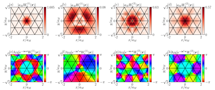
Figure 10: The amplitude (a)-(d) and phase (e)-(h) of maximally localized Wannier states at $+K$ valley. Parameter values are the same as those used for Fig. 2(f).

Appendix E Maximally localized Wannier states

We construct the maximally localized Wannier states by following the method in Refs. 60, 61. We take the Wannier states presented in Sec. IV as the initial guess, and then minimize the spread of the Wannier states. The obtained maximally localized Wannier states are illustrated in Fig. 10. It can be verified that the maximally localized Wannier states remain symmetric under the $C_{3}$ and $M_{x}\mathcal{T}$ symmetries.

The spread of the Wannier states is characterized by

$$\Omega=\sum_{n=1,2}\langle W^{(n)}|\bm{r}^{2}|W^{(n)}\rangle-(\langle W^{(n)}|\bm{r}|W^{(n)}\rangle)^{2},$$ (52)

where $W^{(n)}$ denotes the Wannier states. The spread $\Omega$ is $1.744a_{M}^{2}$ before the optimization and reduced to $1.347a_{M}^{2}$ after the optimization for parameters used in Fig. 4. As shown in Figs. 4 and 10, the optimization only leads to quantitative changes in the Wannier states.

References

• Cao et al. [2018a] Y. Cao, V. Fatemi, A. Demir, S. Fang, S. L. Tomarken, J. Y. Luo, J. D. Sanchez-Yamagishi, K. Watanabe, T. Taniguchi, E. Kaxiras, R. C. Ashoori, and P. Jarillo-Herrero, Correlated insulator behaviour at half-filling in magic-angle graphene superlattices, Nature 556, 80 (2018a).
• Cao et al. [2018b] Y. Cao, V. Fatemi, S. Fang, K. Watanabe, T. Taniguchi, E. Kaxiras, and P. Jarillo-Herrero, Unconventional superconductivity in magic-angle graphene superlattices, Nature 556, 43 (2018b).
• Xu and Balents [2018] C. Xu and L. Balents, Topological Superconductivity in Twisted Multilayer Graphene, Phys. Rev. Lett. 121, 087001 (2018).
• Po et al. [2018] H. C. Po, L. Zou, A. Vishwanath, and T. Senthil, Origin of Mott Insulating Behavior and Superconductivity in Twisted Bilayer Graphene, Phys. Rev. X 8, 031089 (2018).
• Liu et al. [2018] C.-C. Liu, L.-D. Zhang, W.-Q. Chen, and F. Yang, Chiral Spin Density Wave and $d+id$ Superconductivity in the Magic-Angle-Twisted Bilayer Graphene, Phys. Rev. Lett. 121, 217001 (2018).
• Isobe et al. [2018] H. Isobe, N. F. Q. Yuan, and L. Fu, Unconventional Superconductivity and Density Waves in Twisted Bilayer Graphene, Phys. Rev. X 8, 041041 (2018).
• Wu et al. [2018a] F. Wu, A. H. MacDonald, and I. Martin, Theory of Phonon-Mediated Superconductivity in Twisted Bilayer Graphene, Phys. Rev. Lett. 121, 257001 (2018a).
• Yankowitz et al. [2019] M. Yankowitz, S. Chen, H. Polshyn, Y. Zhang, K. Watanabe, T. Taniguchi, D. Graf, A. F. Young, and C. R. Dean, Tuning superconductivity in twisted bilayer graphene, Science 363, 1059 (2019).
• Wu et al. [2019a] F. Wu, E. Hwang, and S. Das Sarma, Phonon-induced giant linear-in-$T$ resistivity in magic angle twisted bilayer graphene: Ordinary strangeness and exotic superconductivity, Phys. Rev. B 99, 165112 (2019a).
• Wu [2019] F. Wu, Topological chiral superconductivity with spontaneous vortices and supercurrent in twisted bilayer graphene, Phys. Rev. B 99, 195114 (2019).
• Lian et al. [2019] B. Lian, Z. Wang, and B. A. Bernevig, Twisted Bilayer Graphene: A Phonon-Driven Superconductor, Phys. Rev. Lett. 122, 257002 (2019).
• Chen et al. [2019] G. Chen, A. L. Sharpe, P. Gallagher, I. T. Rosen, E. J. Fox, L. Jiang, B. Lyu, H. Li, K. Watanabe, T. Taniguchi, J. Jung, Z. Shi, D. Goldhaber-Gordon, Y. Zhang, and F. Wang, Signatures of tunable superconductivity in a trilayer graphene moiré superlattice, Nature 572, 215 (2019).
• Codecido et al. [2019] E. Codecido, Q. Wang, R. Koester, S. Che, H. Tian, R. Lv, S. Tran, K. Watanabe, T. Taniguchi, F. Zhang, M. Bockrath, and C. N. Lau, Correlated insulating and superconducting states in twisted bilayer graphene below the magic angle, Science Advances 5, eaaw9770 (2019).
• Shen et al. [2020] C. Shen, Y. Chu, Q. Wu, N. Li, S. Wang, Y. Zhao, J. Tang, J. Liu, J. Tian, K. Watanabe, T. Taniguchi, R. Yang, Z. Y. Meng, D. Shi, O. V. Yazyev, and G. Zhang, Correlated states in twisted double bilayer graphene, Nature Physics 16, 520 (2020).
• Saito et al. [2020] Y. Saito, J. Ge, K. Watanabe, T. Taniguchi, and A. F. Young, Independent superconductors and correlated insulators in twisted bilayer graphene, Nature Physics 16, 926 (2020).
• Stepanov et al. [2020] P. Stepanov, I. Das, X. Lu, A. Fahimniya, K. Watanabe, T. Taniguchi, F. H. L. Koppens, J. Lischner, L. Levitov, and D. K. Efetov, Untying the insulating and superconducting orders in magic-angle graphene, Nature 583, 375 (2020).
• Yuan and Fu [2018] N. F. Q. Yuan and L. Fu, Model for the metal-insulator transition in graphene superlattices and beyond, Phys. Rev. B 98, 045103 (2018).
• Wu et al. [2018b] F. Wu, T. Lovorn, E. Tutuc, and A. H. MacDonald, Hubbard Model Physics in Transition Metal Dichalcogenide Moiré Bands, Phys. Rev. Lett. 121, 026402 (2018b).
• Koshino et al. [2018] M. Koshino, N. F. Q. Yuan, T. Koretsune, M. Ochi, K. Kuroki, and L. Fu, Maximally Localized Wannier Orbitals and the Extended Hubbard Model for Twisted Bilayer Graphene, Phys. Rev. X 8, 031087 (2018).
• Regan et al. [2020] E. C. Regan, D. Wang, C. Jin, M. I. Bakti Utama, B. Gao, X. Wei, S. Zhao, W. Zhao, Z. Zhang, K. Yumigeta, M. Blei, J. D. Carlström, K. Watanabe, T. Taniguchi, S. Tongay, M. Crommie, A. Zettl, and F. Wang, Mott and generalized Wigner crystal states in WSe2/WS2 moiré superlattices, Nature 579, 359 (2020).
• Tang et al. [2020] Y. Tang, L. Li, T. Li, Y. Xu, S. Liu, K. Barmak, K. Watanabe, T. Taniguchi, A. H. MacDonald, J. Shan, and K. F. Mak, Simulation of Hubbard model physics in WSe2/WS2 moiré superlattices, Nature 579, 353 (2020).
• Xie and MacDonald [2020] M. Xie and A. H. MacDonald, Nature of the Correlated Insulator States in Twisted Bilayer Graphene, Phys. Rev. Lett. 124, 097601 (2020).
• Liu et al. [2020] X. Liu, Z. Hao, E. Khalaf, J. Y. Lee, Y. Ronen, H. Yoo, D. Haei Najafabadi, K. Watanabe, T. Taniguchi, A. Vishwanath, and P. Kim, Tunable spin-polarized correlated states in twisted double bilayer graphene, Nature 583, 221 (2020).
• Li et al. [2021a] H. Li, S. Li, E. C. Regan, D. Wang, W. Zhao, S. Kahn, K. Yumigeta, M. Blei, T. Taniguchi, K. Watanabe, S. Tongay, A. Zettl, M. F. Crommie, and F. Wang, Imaging two-dimensional generalized Wigner crystals, Nature 597, 650 (2021a).
• Wu et al. [2017] F. Wu, T. Lovorn, and A. H. MacDonald, Topological Exciton Bands in Moiré Heterojunctions, Phys. Rev. Lett. 118, 147401 (2017).
• Zou et al. [2018] L. Zou, H. C. Po, A. Vishwanath, and T. Senthil, Band structure of twisted bilayer graphene: Emergent symmetries, commensurate approximants, and Wannier obstructions, Phys. Rev. B 98, 085435 (2018).
• Wu et al. [2019b] F. Wu, T. Lovorn, E. Tutuc, I. Martin, and A. H. MacDonald, Topological Insulators in Twisted Transition Metal Dichalcogenide Homobilayers, Phys. Rev. Lett. 122, 086402 (2019b).
• Po et al. [2019] H. C. Po, L. Zou, T. Senthil, and A. Vishwanath, Faithful tight-binding models and fragile topology of magic-angle bilayer graphene, Phys. Rev. B 99, 195455 (2019).
• Song et al. [2019] Z. Song, Z. Wang, W. Shi, G. Li, C. Fang, and B. A. Bernevig, All Magic Angles in Twisted Bilayer Graphene are Topological, Phys. Rev. Lett. 123, 036401 (2019).
• Sharpe et al. [2019] A. L. Sharpe, E. J. Fox, A. W. Barnard, J. Finney, K. Watanabe, T. Taniguchi, M. A. Kastner, and D. Goldhaber-Gordon, Emergent ferromagnetism near three-quarters filling in twisted bilayer graphene, Science 365, 605 (2019).
• Chen et al. [2020] G. Chen, A. L. Sharpe, E. J. Fox, Y.-H. Zhang, S. Wang, L. Jiang, B. Lyu, H. Li, K. Watanabe, T. Taniguchi, Z. Shi, T. Senthil, D. Goldhaber-Gordon, Y. Zhang, and F. Wang, Tunable correlated Chern insulator and ferromagnetism in a moiré superlattice, Nature 579, 56 (2020).
• Serlin et al. [2020] M. Serlin, C. L. Tschirhart, H. Polshyn, Y. Zhang, J. Zhu, K. Watanabe, T. Taniguchi, L. Balents, and A. F. Young, Intrinsic quantized anomalous Hall effect in a moiré heterostructure, Science 367, 900 (2020).
• Chen et al. [2021] S. Chen, M. He, Y.-H. Zhang, V. Hsieh, Z. Fei, K. Watanabe, T. Taniguchi, D. H. Cobden, X. Xu, C. R. Dean, and M. Yankowitz, Electrically tunable correlated and topological states in twisted monolayer–bilayer graphene, Nature Physics 17, 374 (2021).
• Polshyn et al. [2020] H. Polshyn, J. Zhu, M. A. Kumar, Y. Zhang, F. Yang, C. L. Tschirhart, M. Serlin, K. Watanabe, T. Taniguchi, A. H. MacDonald, and A. F. Young, Electrical switching of magnetic order in an orbital Chern insulator, Nature 588, 66 (2020).
• Nuckolls et al. [2020] K. P. Nuckolls, M. Oh, D. Wong, B. Lian, K. Watanabe, T. Taniguchi, B. A. Bernevig, and A. Yazdani, Strongly correlated Chern insulators in magic-angle twisted bilayer graphene, Nature 588, 610 (2020).
• Das et al. [2021] I. Das, X. Lu, J. Herzog-Arbeitman, Z.-D. Song, K. Watanabe, T. Taniguchi, B. A. Bernevig, and D. K. Efetov, Symmetry-broken Chern insulators and Rashba-like Landau-level crossings in magic-angle bilayer graphene, Nature Physics 17, 710 (2021).
• Stepanov et al. [2021] P. Stepanov, M. Xie, T. Taniguchi, K. Watanabe, X. Lu, A. H. MacDonald, B. A. Bernevig, and D. K. Efetov, Competing Zero-Field Chern Insulators in Superconducting Twisted Bilayer Graphene, Phys. Rev. Lett. 127, 197701 (2021).
• Polshyn et al. [2022] H. Polshyn, Y. Zhang, M. A. Kumar, T. Soejima, P. Ledwith, K. Watanabe, T. Taniguchi, A. Vishwanath, M. P. Zaletel, and A. F. Young, Topological charge density waves at half-integer filling of a moiré superlattice, Nature Physics 18, 42 (2022).
• Xu et al. [2020] Y. Xu, S. Liu, D. A. Rhodes, K. Watanabe, T. Taniguchi, J. Hone, V. Elser, K. F. Mak, and J. Shan, Correlated insulating states at fractional fillings of moiré superlattices, Nature 587, 214 (2020).
• Wang et al. [2020] L. Wang, E.-M. Shih, A. Ghiotto, L. Xian, D. A. Rhodes, C. Tan, M. Claassen, D. M. Kennes, Y. Bai, B. Kim, K. Watanabe, T. Taniguchi, X. Zhu, J. Hone, A. Rubio, A. N. Pasupathy, and C. R. Dean, Correlated electronic phases in twisted bilayer transition metal dichalcogenides, Nature Materials 19, 861 (2020).
• Li et al. [2021b] T. Li, S. Jiang, B. Shen, Y. Zhang, L. Li, Z. Tao, T. Devakul, K. Watanabe, T. Taniguchi, L. Fu, J. Shan, and K. F. Mak, Quantum anomalous Hall effect from intertwined moiré bands, Nature 600, 641 (2021b).
• Zhang et al. [2021] Y. Zhang, T. Devakul, and L. Fu, Spin-textured Chern bands in AB-stacked transition metal dichalcogenide bilayers, Proc. Natl. Acad. Sci. U.S.A. 118, e2112673118 (2021).
• Zhao et al. [2022] W. Zhao, K. Kang, L. Li, C. Tschirhart, E. Redekop, K. Watanabe, T. Taniguchi, A. Young, J. Shan, and K. F. Mak, Realization of the Haldane Chern insulator in a moiré lattice, arXiv:2207.02312  (2022).
• Pan et al. [2022] H. Pan, M. Xie, F. Wu, and S. Das Sarma, Topological Phases in AB-Stacked MoTe2/WSe2 : $\mathbb{Z}_{2}$ Topological Insulators, Chern Insulators, and Topological Charge Density Waves, Phys. Rev. Lett. 129, 056804 (2022).
• Xie et al. [2022] Y.-M. Xie, C.-P. Zhang, J.-X. Hu, K. F. Mak, and K. T. Law, Valley-Polarized Quantum Anomalous Hall State in Moiré ${\text{MoTe}}_{2}/{\text{WSe}}_{2}$ Heterobilayers, Phys. Rev. Lett. 128, 026402 (2022).
• Devakul and Fu [2022] T. Devakul and L. Fu, Quantum Anomalous Hall Effect from Inverted Charge Transfer Gap, Phys. Rev. X 12, 021031 (2022).
• Chang and Chang [2022] Y.-W. Chang and Y.-C. Chang, Quantum anomalous Hall effect and electric-field-induced topological phase transition in AB-stacked ${\mathrm{MoTe}}_{2}/{\mathrm{WSe}}_{2}$ moiré heterobilayers, Phys. Rev. B 106, 245412 (2022).
• Xie et al. [2022a] Y.-M. Xie, C.-P. Zhang, and K. T. Law, Topological $p_{x}+ip_{y}$ inter-valley coherent state in Moiré MoTe2/WSe2 heterobilayers, arXiv:2206.11666  (2022a).
• Xie et al. [2022b] M. Xie, H. Pan, F. Wu, and S. Das Sarma, Nematic excitonic insulator in transition metal dichalcogenide moiré heterobilayers, arXiv:2206.12427  (2022b).
• Dong and Zhang [2022] Z. Dong and Y.-H. Zhang, Excitonic Chern insulator and kinetic ferromagnetism in MoTe2/WSe2 moiré bilayer, arXiv:2206.13567  (2022).
• Tao et al. [2022] Z. Tao, B. Shen, S. Jiang, T. Li, L. Li, L. Ma, W. Zhao, J. Hu, K. Pistunova, K. Watanabe, T. Taniguchi, T. F. Heinz, K. F. Mak, and J. Shan, Valley-coherent quantum anomalous Hall state in AB-stacked MoTe2/WSe2 bilayers, arXiv:2208.07452  (2022).
• Rademaker [2022] L. Rademaker, Spin-orbit coupling in transition metal dichalcogenide heterobilayer flat bands, Phys. Rev. B 105, 195428 (2022).
• Bradlyn et al. [2017] B. Bradlyn, L. Elcoro, J. Cano, M. G. Vergniory, Z. Wang, C. Felser, M. I. Aroyo, and B. A. Bernevig, Topological quantum chemistry, Nature 547, 298 (2017).
• Bernevig et al. [2006] B. A. Bernevig, T. L. Hughes, and S.-C. Zhang, Quantum Spin Hall Effect and Topological Phase Transition in HgTe Quantum Wells, Science 314, 1757 (2006).
• Fang et al. [2012] C. Fang, M. J. Gilbert, and B. A. Bernevig, Bulk topological invariants in noninteracting point group symmetric insulators, Phys. Rev. B 86, 115112 (2012).
• Kane and Mele [2005a] C. L. Kane and E. J. Mele, ${Z}_{2}$ Topological Order and the Quantum Spin Hall Effect, Phys. Rev. Lett. 95, 146802 (2005a).
• Kane and Mele [2005b] C. L. Kane and E. J. Mele, Quantum Spin Hall Effect in Graphene, Phys. Rev. Lett. 95, 226801 (2005b).
• Pan et al. [2020] H. Pan, F. Wu, and S. Das Sarma, Band topology, Hubbard model, Heisenberg model, and Dzyaloshinskii-Moriya interaction in twisted bilayer WSe2Phys. Rev. Research 2, 033087 (2020).
• Devakul et al. [2021] T. Devakul, V. Crépel, Y. Zhang, and L. Fu, Magic in twisted transition metal dichalcogenide bilayers, Nature Communications 12, 6730 (2021).
• Marzari and Vanderbilt [1997] N. Marzari and D. Vanderbilt, Maximally localized generalized Wannier functions for composite energy bands, Phys. Rev. B 56, 12847 (1997).
• Marzari et al. [2012] N. Marzari, A. A. Mostofi, J. R. Yates, I. Souza, and D. Vanderbilt, Maximally localized Wannier functions: Theory and applications, Rev. Mod. Phys. 84, 1419 (2012).