Turbulence via intermolecular potential: A weakly compressible model of gas flow at low Mach number

Abstract.

In our recent works we proposed a theory of turbulence in inertial gas flow via the mean field effect of an intermolecular potential. We found that, in inertial flow, turbulence indeed spontaneously develops from a laminar initial condition, just as observed in nature and experiments. However, we also found that density and temperature in our inertial flow model behave unrealistically. The goal of the current work is to demonstrate technical possibility of modeling compressible, turbulent flow at low Mach number where both density and temperature behave in a more realistic fashion. Here we focus on a new treatment of the pressure variable, which constitutes a compromise between compressible, incompressible and inertial flow. Similarly to incompressible flow, the proposed equation for the pressure variable is artificial, rather than derived directly from kinetic formulation. However, unlike that for incompressible flow, our pressure equation only damps the divergence of velocity, instead of setting it directly to zero. We find that turbulence develops in our weakly compressible model much like it does in the inertial flow model, but density and temperature behave more realistically.

1. Introduction

Observations of turbulence in flows of fluids go at least as far back as Leonardo da Vinci, however, the first mathematical (albeit somewhat primitive) model of turbulent momentum transfer was proposed by Boussinesq [1]. Six years later, Reynolds [2] discovered that an initially laminar flow of water in a straight smooth pipe spontaneously develops turbulent motions whenever the high Reynolds number condition is satisfied, even if all reasonable care is taken to not disturb the flow artificially. Almost sixty years later, Kolmogorov [3, 4, 5] and Obukhov [6] observed that the time-averaged Fourier spectra of the kinetic energy of an atmospheric wind possess universal decay structure, corresponding to the inverse five-thirds power of the Fourier wavenumber. Numerous attempts to explain the physical nature of turbulence have been made throughout the twentieth century [7, 8, 9, 10, 11, 12, 13, 14, 15, 16, 17, 18, 19, 20, 21], yet none successfully. So far, the process of spontaneous turbulence formation in an initially laminar flow, as well as power scaling of turbulent kinetic energy spectra, remained irreproducible, which points to a deficiency in the conventional equations of fluid mechanics. For an example, one can refer to relatively recent works by Avila et al. [22], Barkley et al. [23] and Khan et al. [24], where turbulent-like motions in a numerically simulated flow had to be created via deliberate perturbations.

In our recent works [25, 26, 27, 28] we proposed and investigated a theory of turbulence in a gas, where turbulent motions in an initially laminar, inertial (that is, constant pressure) flow were created via the average effect of gas molecules interacting by means of their intermolecular potential $\phi(r)$. In our theory, this average effect is expressed via the corresponding mean field potential $\bar{\phi}$, and constitutes a density-dependent correction to the pressure gradient in the momentum equation. This effect is absent from the conventional Euler and Navier–Stokes equations of fluid mechanics because, in the Boltzmann–Grad limit [29], it is tacitly assumed that the effect of $\bar{\phi}$ is negligible. However, we found that, in our model of inertial gas flow, turbulent motions spontaneously emerge in the presence of $\bar{\phi}$, while failing to do so in its absence [27].

In the past, a similar idea was proposed by Tsugé [30], who theorized that turbulence was created via long-range correlations between molecules, however, Tsugé’s result was restricted to incompressible flow. Yet, from what we discovered thus far, it appears that turbulence spontaneously emerges from density fluctuations in an initially laminar flow, which means that a model of turbulence must be compressible. In our past work [31], we also considered long-range interactions as a possible reason for the manifestation of turbulence. However, we later observed that even the short-range hard sphere potential creates turbulence in our model, which means that a typical intermolecular potential (e.g. the Lennard-Jones potential [32]) is also capable of the same effect.

At this stage, it is evident from our recent works [25, 26, 27, 28], that spontaneous turbulent motions in an otherwise laminar flow are created by the mean field effect of the intermolecular potential, which thus far was overlooked in the conventional equations of fluid mechanics. However, the new, subsequent, question has arisen in our study, which is how to treat the pressure variable? Conventional equations of fluid mechanics offer two options: either compressible flow, where pressure has its own transport equation, or incompressible flow, where it is artificially set to keep the divergence of velocity at zero. Unfortunately, neither of the two options seems to be compatible with the mechanics of turbulence creation; as we show below, compressible equations generally behave poorly at low Mach number (which is a well known problem), while the structure of incompressible equations precludes turbulence from developing. In our works [25, 26, 27, 28] we suggested a third option of setting the pressure to a constant (inertial flow). However, while turbulent motions indeed develop spontaneously in our inertial flow, we found that the dynamics of density and temperature can be unrealistic.

In the current work, we propose a novel treatment of the pressure variable, which, by its design, constitutes a compromise between compressible, incompressible and inertial flow. Similarly to incompressible flow, the proposed pressure equation is artificial, rather than derived directly from the kinetic formulation. However, unlike that for incompressible flow, our pressure equation only damps the divergence of velocity, instead of setting it directly to zero. In the resulting model, turbulence spontaneously develops from a laminar flow, and, at the same time, density and temperature behave more realistically.

The work is organized as follows. In Section 2 we propose a model for weakly compressible flow. In Section 3 we describe the computational implementation of the proposed model. In Section 4 we present the results of our numerical experiment with the proposed model. Section 5 summarizes the results of the work.

2. A new model of weakly compressible flow

For convenience, here we start with introducing the advective (or “material”) derivative operator for the flow velocity $\boldsymbol{u}$, given via

(2.1) $$\frac{\mathrm{D}f}{\mathrm{D}t}\equiv\frac{\partial f}{\partial t}+\boldsymbol{u}\cdot\nabla f,$$

whose geometric meaning is the directional derivative with respect to time $t$ along the direction of the flow. With the help of this operator, the transport equations for the density $\rho$ and velocity $\boldsymbol{u}$ are written, respectively, via

(2.2) $$\frac{\mathrm{D}\rho}{\mathrm{D}t}=-\rho\nabla\cdot\boldsymbol{u},\qquad\rho\frac{\mathrm{D}\boldsymbol{u}}{\mathrm{D}t}=-\nabla(p+\bar{\phi})+\nabla\cdot(\mu\nabla\boldsymbol{u}),$$

where $p$, $\mu$ and $\bar{\phi}$ are the pressure, viscosity and the mean field potential, respectively. The latter has been introduced in our recent works [25, 26, 27, 28], and is not a part of the conventional fluid mechanics equations. The general formula for the mean field potential $\bar{\phi}$ is given [27] via

(2.3) $$\bar{\phi}=\frac{2\pi p\rho}{3m}\int_{0}^{\infty}\big{(}1-e^{-\phi(r)/\theta}\big{)}\frac{\partial}{\partial r}\big{(}r^{3}Y(r)\big{)}\>\!\mathrm{d}r,$$

where $m$ is the mass of a gas molecule, $\phi(r)$ is the short-range intermolecular potential, $\theta=p/\rho$ is the kinetic temperature, and $Y(r)$ is the cavity distribution function [33] for a pair of molecules. Under the assumption that the gas is sufficiently dilute (i.e. $Y\approx 1$), and that the intermolecular potential $\phi(r)$ can be approximated via the hard sphere potential $\phi_{HS}$ with effective range $\sigma$, that is,

(2.4) $$\phi_{HS}(r)=\left\{\begin{array}[]{l@{,\qquad}l@{,}}\infty&r\leq\sigma\\ 0&r>\sigma\end{array}\right.$$

the general formula in (2.3) simplifies to

(2.5) $$\bar{\phi}_{HS}=\frac{4\rho p}{\rho_{HS}}.$$

Above, $\rho_{HS}=6m/\pi\sigma^{3}$ is the density of an equivalent hard sphere of mass $m$ and diameter $\sigma$. Upon substitution of (2.5) into (2.2), we arrive at

(2.6) $$\frac{\mathrm{D}\rho}{\mathrm{D}t}=-\rho\nabla\cdot\boldsymbol{u},\qquad\rho\frac{\mathrm{D}\boldsymbol{u}}{\mathrm{D}t}=-\nabla\left[p\left(1+\frac{4\rho}{\rho_{HS}}\right)\right]+\nabla\cdot(\mu\nabla\boldsymbol{u}).$$

Thus far, the pressure $p$ is the only variable which lacks an equation. This is intentional; while the transport equations for the density and velocity variables are universal, the treatment of the pressure variable depends on the dynamical regime of the flow.

In compressible flow at high Mach number, the pressure $p$ is equipped with its own transport equation, which is derived from the Boltzmann equation by computing velocity moments of the distribution function [34, 35]:

(2.7) $$\frac{1}{\gamma}\frac{\mathrm{D}p}{\mathrm{D}t}=-p\nabla\cdot\boldsymbol{u}+\nabla\cdot\left(\frac{\mu}{\mathit{Pr}}\nabla\theta\right).$$

Above, $\gamma$ and $\mathit{Pr}$ are the adiabatic exponent and the Prandtl number, respectively, and we also forgo the stress term for simplicity. The equations in (2.6) (with $\rho_{HS}$ set to infinity) and (2.7), taken together as a system, comprise the standard compressible Navier–Stokes equations [36, 37]. However, it is well known that these compressible equations do not constitute an accurate model of compressible flow at low Mach and high Reynolds numbers. In particular, if one attempts to model such a flow via a numerical simulation, the resulting numerical solution will be inundated with unrealistic amounts of acoustic waves, which clearly does not happen in nature.

2.1. Rescaling and non-dimensionalization

The reason for inaccurate behavior of the system in (2.6) and (2.7) at low Mach number can be seen with the help of a standard rescaling of variables. To this end, we introduce reference constants $L$ and $U$, which correspond to the spatial scale of the problem, and the characteristic speed of the flow, respectively. We then rescale the variables $\boldsymbol{x}$, $t$ and $\boldsymbol{u}$ as follows:

(2.8) $$\boldsymbol{x}=L\boldsymbol{\tilde{x}},\qquad t=\frac{L}{U}\tilde{t},\qquad\boldsymbol{u}=U\boldsymbol{\tilde{u}}.$$

It is easy to see that the advective derivative is rescaled via

(2.9) $$\frac{\mathrm{D}f}{\mathrm{D}t}=\frac{U}{L}\frac{\mathrm{D}f}{\mathrm{D}\tilde{t}}.$$

In addition, we introduce reference density $\rho_{0}$, temperature $T_{0}$ (in degrees K), and viscosity $\mu_{0}$. The corresponding rescalings for $\rho$, $p$ and $\mu$ are given via

(2.10) $$\rho=\rho_{0}\tilde{\rho},\qquad p=\rho_{0}\theta_{0}\tilde{p},\qquad\mu=\mu_{0}\tilde{\mu},\qquad\theta_{0}=\frac{RT_{0}}{M},$$

where $R$ and $M$ are the universal gas constant and the molar mass of gas, respectively. Upon substitution into (2.6) and (2.7), we obtain the following non-dimensional equations:

(2.11a) $$\frac{\mathrm{D}\tilde{\rho}}{\mathrm{D}\tilde{t}}=-\tilde{\rho}\tilde{\nabla}\cdot\boldsymbol{\tilde{u}},\qquad\tilde{\rho}\frac{\mathrm{D}\boldsymbol{\tilde{u}}}{\mathrm{D}\tilde{t}}=-\frac{1}{\mathit{Ma}^{2}}\tilde{\nabla}\tilde{p}-\frac{4\eta}{\mathit{Ma}^{2}}\tilde{\nabla}(\tilde{\rho}\tilde{p})+\frac{1}{\mathit{Re}}\tilde{\nabla}\cdot(\tilde{\mu}\tilde{\nabla}\boldsymbol{\tilde{u}}),$$

(2.11b) $$\frac{1}{\gamma}\frac{\mathrm{D}\tilde{p}}{\mathrm{D}\tilde{t}}=-\tilde{p}\tilde{\nabla}\cdot\boldsymbol{\tilde{u}}+\frac{1}{\mathit{Re}}\tilde{\nabla}\cdot\left(\frac{\tilde{\mu}}{\mathit{Pr}}\tilde{\nabla}\tilde{\theta}\right).$$

Above, $\mathit{Ma}$, $\mathit{Re}$ and $\eta$ are, respectively, the Mach number, the Reynolds number, and the packing fraction:

(2.12) $$\mathit{Ma}=\frac{U}{\sqrt{\theta_{0}}},\qquad\mathit{Re}=\frac{\rho_{0}UL}{\mu_{0}},\qquad\eta=\frac{\rho_{0}}{\rho_{HS}}.$$

At normal conditions, the packing fraction $\eta\sim 10^{-3}$ [26]. As a result, for typical low Mach number values, say, $\mathit{Ma}\sim 0.1$ (which corresponds to $U\sim$ 30 m/s at normal conditions), we have $\mathit{Ma}^{2}\ll 1$, while $4\eta/\mathit{Ma}^{2}\sim 1$. Additionally, for a flow to be turbulent, $\mathit{Re}\gg 1$ (see Reynolds [2]). It is thus apparent that, at low Mach numbers, the term with the pressure gradient dominates the momentum equation, if the non-dimensional pressure gradient itself is $\tilde{\nabla}\tilde{p}\sim 1$.

However, it is known from observations that gas flows at normal conditions and low Mach number do not exhibit any irregular behavior. This, in turn, means that, in order for the rescaled equations in (2.11) to accurately model real gas flows, the non-dimensional pressure gradient must at least satisfy $\tilde{\nabla}\tilde{p}\lesssim O(\mathit{Ma}^{2})$. However, at high Reynolds number, it can only happen, at least on the non-dimensional time scale $\tilde{t}\sim 1$, if $\tilde{\nabla}\cdot\boldsymbol{\tilde{u}}\sim O(\mathit{Ma}^{2})$. Irrespectively of physics, there are two principal technical approaches to control the gradient of the pressure:

• The direct approach: explicitly set the pressure gradient to a desired value (such as zero);

• The indirect approach: implicitly control the pressure gradient by appropriately restricting the magnitude of velocity divergence.

We already tested the direct approach in our recent works [25, 26, 27, 28] by setting the pressure variable to a constant, thus modeling inertial flow. Although this, rather primitive, model indeed reproduces main features of turbulent flow, there are some aspects of it which are unrealistic – in particular, variations of density and temperature are much larger than what is typically observed.

A form of the indirect approach is used in the conventional equations for incompressible flow, where the divergence of flow velocity is preserved along a streamline via an artificial choice of the pressure equation. Coupled with a divergence-free initial condition, the equations for incompressible flow produce solutions which tend to behave regularly at low Mach number. However, below we show that this approach is unsuitable for our purpose, because turbulent dynamics are not retained in the equations for incompressible flow.

2.2. Incompressible flow

A conventional way to control the divergence of velocity at low Mach number is to replace the pressure transport equation in (2.7) with an artificial constitutive relation, which deliberately sets the pressure in such a way so as to preserve the divergence of velocity along a streamline, which leads to the incompressible Navier–Stokes equations [36]. The same procedure can in fact also be used for our momentum equation in (2.6) with the additional mean field potential term. In order to proceed, first observe that, if we somehow ensure that $\nabla\cdot\boldsymbol{u}=0$, then constant density $\rho=\rho_{0}$ becomes a valid solution. Thus, presuming that the density variable is constant, we can write the momentum equation in (2.6) in the form

(2.13) $$\rho_{0}\frac{\mathrm{D}\boldsymbol{u}}{\mathrm{D}t}=-(1+4\eta)\nabla p+\nabla\cdot(\mu\nabla\boldsymbol{u}).$$

Let us now compute the divergence of both sides of the equation above, and, in addition, presume that viscosity $\mu=\mu_{0}$ is also constant:

(2.14) $$\rho_{0}\nabla\cdot\frac{\mathrm{D}\boldsymbol{u}}{\mathrm{D}t}=-(1+4\eta)\Delta p+\mu_{0}\Delta(\nabla\cdot\boldsymbol{u}).$$

Next, observe that

(2.15) $$\nabla\cdot\frac{\mathrm{D}\boldsymbol{u}}{\mathrm{D}t}=\frac{\partial(\nabla\cdot\boldsymbol{u})}{\partial t}+\nabla\cdot(\boldsymbol{u}\cdot\nabla\boldsymbol{u})=\frac{\mathrm{D}(\nabla\cdot\boldsymbol{u})}{\mathrm{D}t}+\nabla\boldsymbol{u}^{T}:\nabla\boldsymbol{u},$$

where “$:$” denotes the Frobenius product of two matrices. This leads to

(2.16) $$\rho_{0}\left(\frac{\mathrm{D}(\nabla\cdot\boldsymbol{u})}{\mathrm{D}t}+\nabla\boldsymbol{u}^{T}:\nabla\boldsymbol{u}\right)=-(1+4\eta)\Delta p+\mu_{0}\Delta(\nabla\cdot\boldsymbol{u}).$$

It is now clear that, in order to preserve $\nabla\cdot\boldsymbol{u}=0$ along the streamline, the pressure must satisfy

(2.17) $$\Delta p=-\frac{\rho_{0}}{1+4\eta}\nabla\boldsymbol{u}^{T}:\nabla\boldsymbol{u}.$$

This is the artificial pressure equation in the incompressible setting. In the conventional formulation without the mean field potential forcing, the packing fraction $\eta$ is not present. However, there is otherwise no difference in the dynamics – clearly, the velocity solution is the same for the same initial and boundary conditions, while the pressure variable functions as a “Lagrange multiplier” to ensure that the velocity field is divergence-free. Thus, the presence of the mean field potential does not affect the incompressible dynamics, and, therefore, does not produce turbulent flow.

2.3. New idea: weakly compressible flow

In the current work, we explore a more flexible approach, where the artificial pressure condition is chosen to constitute “middle ground” between the incompressible and inertial regimes. We refer to our new model as weakly compressible flow, because it aims to control the divergence of velocity by damping it, rather than setting it directly to zero.

Let us divide the momentum equation in (2.6) by $\rho$, and compute the divergence on both sides:

(2.18) $$\frac{\mathrm{D}(\nabla\cdot\boldsymbol{u})}{\mathrm{D}t}+\nabla\boldsymbol{u}^{T}:\nabla\boldsymbol{u}=-\nabla\cdot\left(\frac{1}{\rho}\nabla\left[p\left(1+\frac{4\rho}{\rho_{HS}}\right)\right]\right)+\nabla\cdot\left(\rho^{-1}\nabla\cdot(\mu\nabla\boldsymbol{u})\right).$$

After the rescaling and subsequent non-dimensionalization of the variables, the equation above becomes

(2.19) $$\frac{\mathrm{D}(\tilde{\nabla}\cdot\boldsymbol{\tilde{u}})}{\mathrm{D}\tilde{t}}+\tilde{\nabla}\boldsymbol{\tilde{u}}^{T}:\tilde{\nabla}\boldsymbol{\tilde{u}}=-\frac{1}{\mathit{Ma}^{2}}\nabla\cdot\left(\tilde{\rho}^{-1}\nabla\left[\tilde{p}(1+4\eta\tilde{\rho})\right]\right)+\frac{1}{\mathit{Re}}\tilde{\nabla}\cdot\left(\tilde{\rho}^{-1}\tilde{\nabla}\cdot(\tilde{\mu}\tilde{\nabla}\boldsymbol{\tilde{u}})\right).$$

Here, we propose to control the divergence of velocity by imposing linear damping on it via the following artificial pressure equation:

(2.20) $$\tilde{\nabla}\cdot\left(\tilde{\rho}^{-1}\tilde{\nabla}\tilde{p}\right)=\tilde{\tau}^{-1}\tilde{\nabla}\cdot\boldsymbol{\tilde{u}},$$

where $\tilde{\tau}\sim 1$ is the non-dimensional characteristic time of decay, chosen empirically. Then, the balance of terms in the right-hand side of (2.19) is given via

(2.21) $$\frac{\mathrm{D}(\tilde{\nabla}\cdot\boldsymbol{\tilde{u}})}{\mathrm{D}\tilde{t}}+\tilde{\nabla}\boldsymbol{\tilde{u}}^{T}:\tilde{\nabla}\boldsymbol{\tilde{u}}=-\frac{\tilde{\nabla}\cdot\boldsymbol{\tilde{u}}}{\mathit{Ma}^{2}\tilde{\tau}}+O\left(\frac{4\eta}{\mathit{Ma}^{2}}\right)+O\left(\mathit{Re}^{-1}\right),$$

that is, such substitution renders $\tilde{\nabla}\cdot\boldsymbol{\tilde{u}}\sim\mathit{Ma}^{2}$, at least on the non-dimensional time scale $\tilde{t}\sim 1$. Generally, to control the divergence, the right-hand side of (2.20) can be a linear (or even nonlinear) positive definite operator acting on $\tilde{\nabla}\cdot\boldsymbol{\tilde{u}}$, however, here we choose the simplest option in the form of linear damping. As we can see, the proposed pressure equation in (2.20) is completely artificial, just as the one for incompressible flow. However, in our case, the flow remains compressible (even if weakly), and thus still retains the turbulent effect induced by the mean field potential.

2.4. Simplified weakly compressible equations

Reverting back to dimensional variables, and expressing the advection terms in a conservative form, we arrive at

(2.22a) $$\frac{\partial\rho}{\partial t}+\nabla\cdot(\rho\boldsymbol{u})=0,\qquad\nabla\cdot\left(\frac{\tau}{\rho}\nabla p\right)=\nabla\cdot\boldsymbol{u},\qquad\tau=\frac{UL}{\theta_{0}}\tilde{\tau},$$

(2.22b) $$\frac{\partial(\rho\boldsymbol{u})}{\partial t}+\nabla\cdot(\rho\boldsymbol{u}^{2})+\left(1+\frac{4\rho}{\rho_{HS}}\right)\nabla p+\frac{4p}{\rho_{HS}}\nabla\rho=\nabla\cdot(\mu\nabla\boldsymbol{u}).$$

At normal conditions, observe that $\rho/\rho_{HS}\sim 10^{-3}$, which is a small correction to unity. Thus, we discard this small correction in the momentum equation, by setting

(2.23) $$1+4\rho/\rho_{HS}\to 1.$$

Additionally, noting that, at low Mach numbers, the pressure consists largely of its background state $p_{0}$ with small fluctuations, we replace $p$ with $p_{0}$ in the density gradient term of the momentum equation. The resulting simplified, weakly compressible equations are

(2.24a) $$\frac{\partial\rho}{\partial t}+\nabla\cdot(\rho\boldsymbol{u})=0,\qquad\nabla\cdot\left(\frac{\tau}{\rho}\nabla p\right)=\nabla\cdot\boldsymbol{u},\qquad\tau=\frac{UL}{\theta_{0}}\tilde{\tau},$$

(2.24b) $$\frac{\partial(\rho\boldsymbol{u})}{\partial t}+\nabla\cdot(\rho\boldsymbol{u}^{2})+\nabla p+\frac{4p_{0}}{\rho_{HS}}\nabla\rho=\nabla\cdot(\mu\nabla\boldsymbol{u}).$$

Note that, as a result of the simplifications above, the nonlinear coupling between $\rho$ and $p$ in the momentum equation has been eliminated. Also, observe that one can obtain the inertial flow system used in our recent works [25, 26, 27, 28] by setting $\nabla p=\boldsymbol{0}$ in (2.24b) and discarding the pressure equation from (2.24a).

3. Computational implementation of the model

Here we describe the computational implementation of the simplified weakly compressible equations in (2.24). As in our recent works [25, 26, 27, 28], we use OpenFOAM [38] to implement the computational code.

3.1. The time-stepping scheme

The spatial discretization of (2.24) is implemented in OpenFOAM via the standard second-order finite volume scheme using the van Leer flux limiter [39]. However, the time discretization is somewhat nontrivial, because $\nabla p$ in (2.24b) effectively constitutes a linear damping of momentum. It is well known that dissipative linear terms have to be treated implicitly during time stepping to avoid numerical instability. Here, we use a first order stepping with the time step denoted via $\Delta t$,

(3.1a) $$\frac{\rho_{*}-\rho}{\Delta t}+\nabla\cdot(\rho\boldsymbol{u})=0,\qquad\nabla\cdot\left(\frac{\tau}{\rho_{*}}\nabla p_{*}\right)=\nabla\cdot\boldsymbol{u}_{*},$$

(3.1b) $$\frac{\rho_{*}\boldsymbol{u}_{*}-\rho\boldsymbol{u}}{\Delta t}+\nabla\cdot(\rho\boldsymbol{u}\boldsymbol{u}_{*})+\nabla p_{*}+\frac{4p_{0}}{\rho_{HS}}\nabla\rho_{*}=\nabla\cdot(\mu\nabla\boldsymbol{u}_{*}),$$

where the variables subscripted with asterisks refer to the next time level. Above, observe that $\rho_{*}$ can be computed explicitly from the density equation in (3.1a), while $p_{*}$ and $\boldsymbol{u}_{*}$ are coupled into a linear system of equations for pressure in (3.1a) and momentum in (3.1b). We solve this system of equations via an underrelaxed fixed point iteration for the main diagonal of the discretized momentum equation (effectively amounting to a Jacobi iteration). At each time step, the computation proceeds as follows:

1. $\rho_{*}$ is evaluated from the density equation in (3.1a);

2. $\boldsymbol{u}_{*}^{(1)}$ is evaluated from the momentum equation in (3.1b) with $p_{*}^{(0)}=p$;

3. $p_{*}^{(k)}$ is evaluated from the pressure equation in (3.1a) for the current iterate $u_{*}^{(k)}$;

4. $\boldsymbol{u}_{*}^{(k+1)}$ is evaluated from an underrelaxed, diagonally dominant rearrangement of the momentum equation in (3.1b) for the current iterate $p_{*}^{(k)}$;

5. Steps (iii) and (iv) are repeated until the pressure equation in (3.1a) becomes identity for the iterates $p_{*}^{(k)}$ and $\boldsymbol{u}_{*}^{(k)}$, subject to a suitable tolerance. Then, $p_{*}^{(k)}$ and $\boldsymbol{u}_{*}^{(k)}$ are accepted as $p_{*}$ and $\boldsymbol{u}_{*}$, respectively, for the next time step.

In the context of OpenFOAM, the steps above are programmed similarly to the implementation of the PISO algorithm [40] in the standard icoFoam solver.

3.2. Description of the computational domain and parameters

In our recent works [25, 27, 28], the computational domain was a straight pipe of square cross-section, whose spatial discretization consisted of uniform cubes. In the current work, we “upgrade” the domain to be a cylindrical pipe instead, which is easily achievable via the finite-volume discretization, naturally provided by OpenFOAM. The pipe has 48 cm in length, and 7 cm in diameter. The three-dimensional “wire mesh” of the pipe, which illustrates the spatial discretization, is displayed in Figure 1.

In the longitudinal direction, the spatial discretization is uniform with step 0.8 mm, same as in our recent work [27], which, given the length of the pipe, yields 600 spatial discretization steps along the axis of the pipe. The discretization scheme in the transversal plane is shown separately in Figure 2; it consists of the central 2.8$\times$2.8 cm² “core”, with four adjacent quadrangular blocks, whose outer circular edges form the boundary of the pipe. The size of a discretization cell within the central core is 0.8$\times$0.8 mm², such that the core has uniform spatial discretization in all three dimensions. In the transversal plane, the central core contains 35$\times$35=1225 cells, while each of the four adjacent quadrangular blocks contains 35$\times$19=665 cells. Thus, the transversal plane contains 3885 cells in total, and the total number of cells in the domain is 3885$\times$600$=$2 331 000.

Figure 1. General structure of the finite-volume discretization mesh of the cylindrical pipe.

3.3. Initial and boundary conditions, and other parameters of the simulation

In the current work, we simulate air flow at normal conditions. Thus, the background pressure and the hard sphere density are set to $p_{0}=101.3$ kPa and $\rho_{HS}=1850$ kg/m³ [26], respectively. The scaling parameters in (2.24a) are set to $U=$ 30 m/s (the maximum speed difference in the jet), $L=$ 1 cm (the thickness of the jet) and $T_{0}=$ 293.15 K (20 ^∘C). The molar mass of air and the universal gas constant are set to $M=$ 28.97 g/mol and $R=$ 8.31446 kg m²/s² mol K, respectively.

The resulting reference kinetic temperature $\theta_{0}$ and Mach number $\mathit{Ma}$ are given via

(3.2) $$\theta_{0}=\frac{RT_{0}}{M}\approx 8.4\cdot 10^{4}\text{ m}^{2}/\text{s}^{2},\qquad\mathit{Ma}=\frac{U}{\sqrt{\theta_{0}}}\approx 0.1,$$

and we choose the non-dimensional empirical characteristic decay time to be $\tilde{\tau}=$ 2.5. The viscosity variable $\mu$ is set to

(3.3) $$\mu=\mu_{0}\sqrt{\frac{p}{\theta_{0}\rho}},$$

where the reference value of viscosity is set to $\mu_{0}=1.825\cdot 10^{-5}$ kg/m s, to match the viscosity of air at 293.15 K.

Figure 2. The structure of the spatial discretization mesh in the transverse plane of the pipe.

The boundary conditions of flow in the pipe are chosen similarly to those in our recent work [27]. Namely, the front end of the pipe is treated as a wall, which houses a round axisymmetric inlet of 1 cm in diameter. The back end of the pipe represents the outlet of the flow. The model variables are specified at the boundaries as follows:

• Inlet and walls: The Dirichlet boundary condition is set for velocity and temperature. The velocity variable has zero value at the walls, and a radially symmetric parabolic profile at the inlet, with the maximum value of 30 m/s at the center (as in the experiment of Buchhave and Velte [41]), directed along the longitudinal axis of the pipe. The temperature variable is set to 293.15 K at the inlet and the walls. The Neumann boundary condition (zero normal derivative) is specified for pressure.

• Outlet: For velocity and temperature, we set the Neumann boundary condition with zero normal derivative. The pressure variable is set to 101.3 kPa, which constitutes the Dirichlet boundary condition.

The initial state of the flow within the pipe is set as follows: the temperature and pressure variables are prescribed constant values of 293.15 K and 101.3 kPa, respectively, while the velocity variable is set to the laminar axisymmetric jet with parabolic profile matching the inlet boundary condition, which extends throughout the length of the pipe.

4. Results of the numerical simulation

Here we report the results of the numerical simulation of air flow within the cylindrical pipe, described above. What follows is separated into two parts: first, we demonstrate how turbulent flow develops from a laminar initial condition, and, second, we present the properties of fully developed turbulent flow. The snapshots of various quantities in Figures 3–7 are produced with help of ParaView, while the kinetic energy spectra in Figure 8 are computed and visualized using Octave.

4.1. Development of turbulent flow from a laminar initial condition

As Reynolds first observed in his experiment [2], the development of turbulence is characterized by spontaneous disintegration of laminar flow into chaotic motions across multiple scales. Thus, in Figure 3 we present the lateral view of the pipe, with velocity displayed as a vector field at times $t=$ 0.01, 0.02, 0.03, 0.04 and 0.05. The direction of arrows in Figure 3 correspond to the direction of flow velocity , while their length and color-coding match the flow speed in that location. As we can see, the initially laminar jet spontaneously transitions into chaotic flow on the time scale of 0.05 seconds. This is similar to what we observed in our recent works [25, 26, 27, 28].

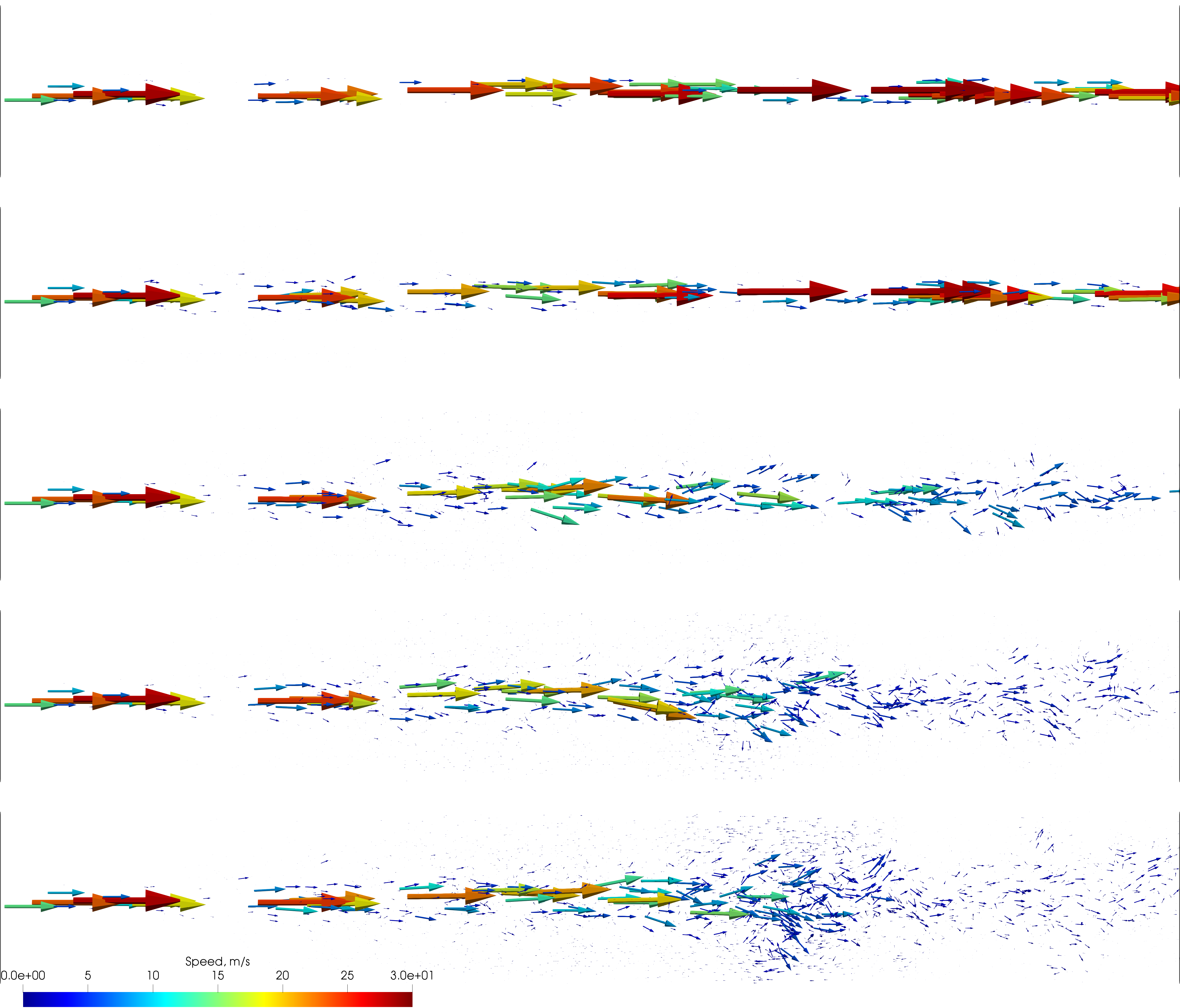
Figure 3. Velocity of the flow at times $t=0.01$, $0.02$, $0.03$, $0.04$ and $0.05$ s (top to bottom).

Figure 4. The density of the passive tracer at times $t=0.01$, $0.02$, $0.03$, $0.04$ and $0.05$ s (top to bottom).

While the velocity plots are quite illustrative, in practical observations the onset of turbulence is usually detected via a passive tracer – that is, a visually detectable substance, which is deliberately added to a gas or a liquid. This substance is chosen to be physically and chemically inert, to avoid interference with the dynamics of the flow. Here, we simulate the propagation of the passive tracer using the corresponding equation

(4.1) $$\frac{\partial(\rho s)}{\partial t}+\nabla\cdot(\rho s\boldsymbol{u})=0,$$

where $s=s(t,\boldsymbol{x})$ is the density of the tracer substance. We set the inlet boundary condition for $s$ to be of the Dirichlet type, with $s=1$ within 0.2 cm distance from the longitudinal axis, and zero otherwise (such that the initial diameter of the resulting streak is 0.4 cm). In Figure 4 we again present the lateral view of the pipe, where the density of the passive tracer is displayed at times $t=$ 0.01, 0.02, 0.03, 0.04 and 0.05. With help of ParaView, the plots in Figure 4 are produced via level surfaces of the tracer density, distributed logarithmically from 0.01 to 1, with the opacity of each level surface set proportionally to the corresponding value of $s$. The logarithmic distribution of level surfaces is chosen to mimic the logarithmic sensitivity of a human eye, for a more natural visualization. Again, we can see that the initially laminar streak of the passive tracer spontaneously dissolves into the surrounding flow, as typically observed in experiments (e.g. Reynolds [2], p. 942, Fig. 4).

4.2. Properties of fully developed turbulent flow

In the current computational setting, we observed that turbulent flow fully develops at the elapsed time $t=$ 0.15 s (that is, its statistical properties do not appear to change noticeably thereafter). Thus, in Figure 5 we show velocity of the flow and density of the passive tracer at time $t=$ 0.15 s, in the same fashion as in Figures 3 and 4 above. Observe that velocity has largely same pattern as at $t=$ 0.05 s, except that the complete breakdown of the jet occurs somewhat closer to the inlet (approximately in the middle of the pipe, or $\sim$ 24 cm from the inlet). The density of the passive tracer exhibits matching behavior; namely, it has laminar structure roughly for the first third of the length of the pipe, and then rather abruptly breaks down into a partially transparent cloud, inside which more dense structures are visible. Such behavior appears to be similar to what was observed by Reynolds, even though he experimented with turbulent flow of water, rather than air.

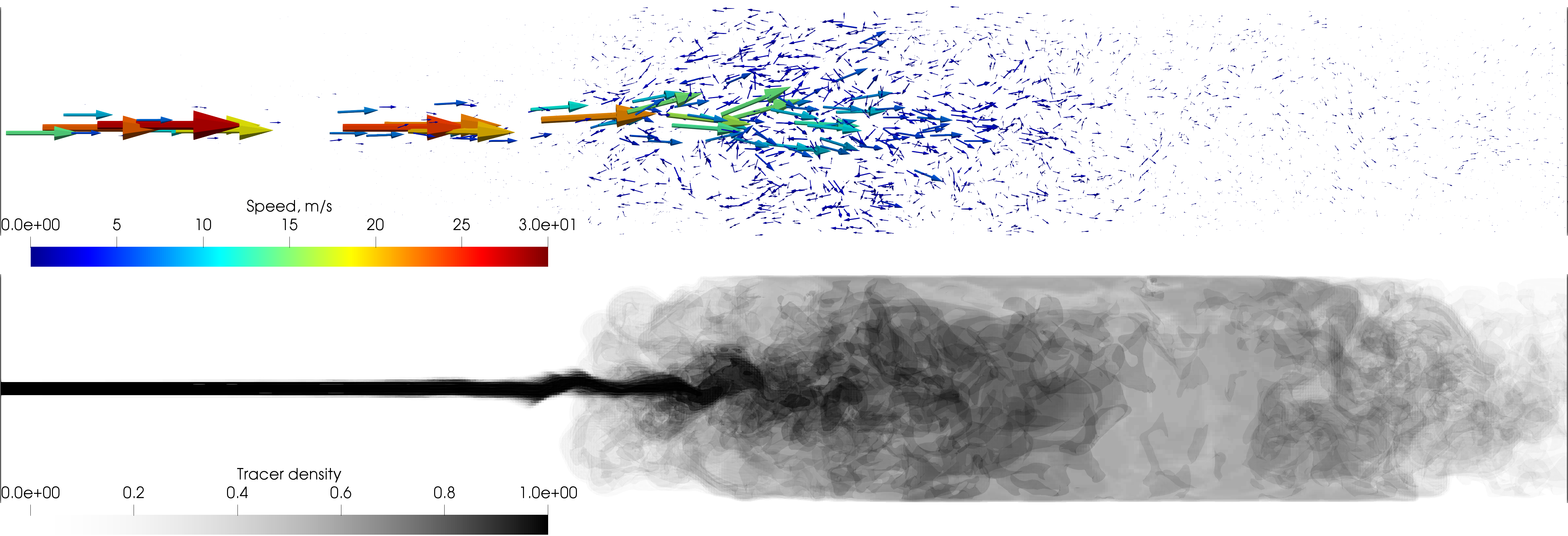
Figure 5. Velocity of the flow (top) and density of the passive tracer (bottom) at time $t=0.15$ s.

In Figure 6 we show the magnitude of pressure gradient $\|\nabla p\|$, the divergence of flow velocity $\nabla\cdot\boldsymbol{u}$, and compare the latter with the magnitude of vorticity $\|\nabla\times\boldsymbol{u}\|$. All three plots are made as follows: first, a set of uniformly (rather than logarithmically, as was the case for the passive tracer) distributed color-coded level surfaces is created in ParaView. Then, all parts of these level surfaces which are in front of the lateral plane of the pipe are deleted, thus revealing the “intestines” of the plot.

By design, the weakly compressible system in (2.24) aims to keep the non-dimensional pressure gradient and the velocity divergence at about $O(\mathit{Ma}^{2})$, while lacking direct mechanisms to restrict vorticity. Observe that the magnitude of the pressure gradient reaches, at the extreme, 20 kPa/m, which in the non-dimensional units (that is, after multiplying by $L/p_{0}$, with $L=$ 1 cm and $p_{0}=$ 101.3 kPa) constitutes $\sim$ 0.002, that is, clearly below $\mathit{Ma}^{2}$. Thus, the primary goal of (2.24) is achieved – the pressure gradient in the momentum equation (2.24b) does not become large at given Mach number. Additionally, observe that such extreme values of the pressure gradient are reached only in a few localized spots in the domain, whereas its bulk values are clearly much lower. In particular, the average value of $\|\nabla p\|$ over the domain is

(4.2) $$\frac{1}{V}\int_{D}\|\nabla p\|\>\!\mathrm{d}\boldsymbol{x}=210\text{ Pa}/\text{m},$$

where $V$ signifies the volume of the pipe, and which in the non-dimensional units totals $2.1\cdot 10^{-5}$, that is, much lower than $\mathit{Ma}^{2}$.

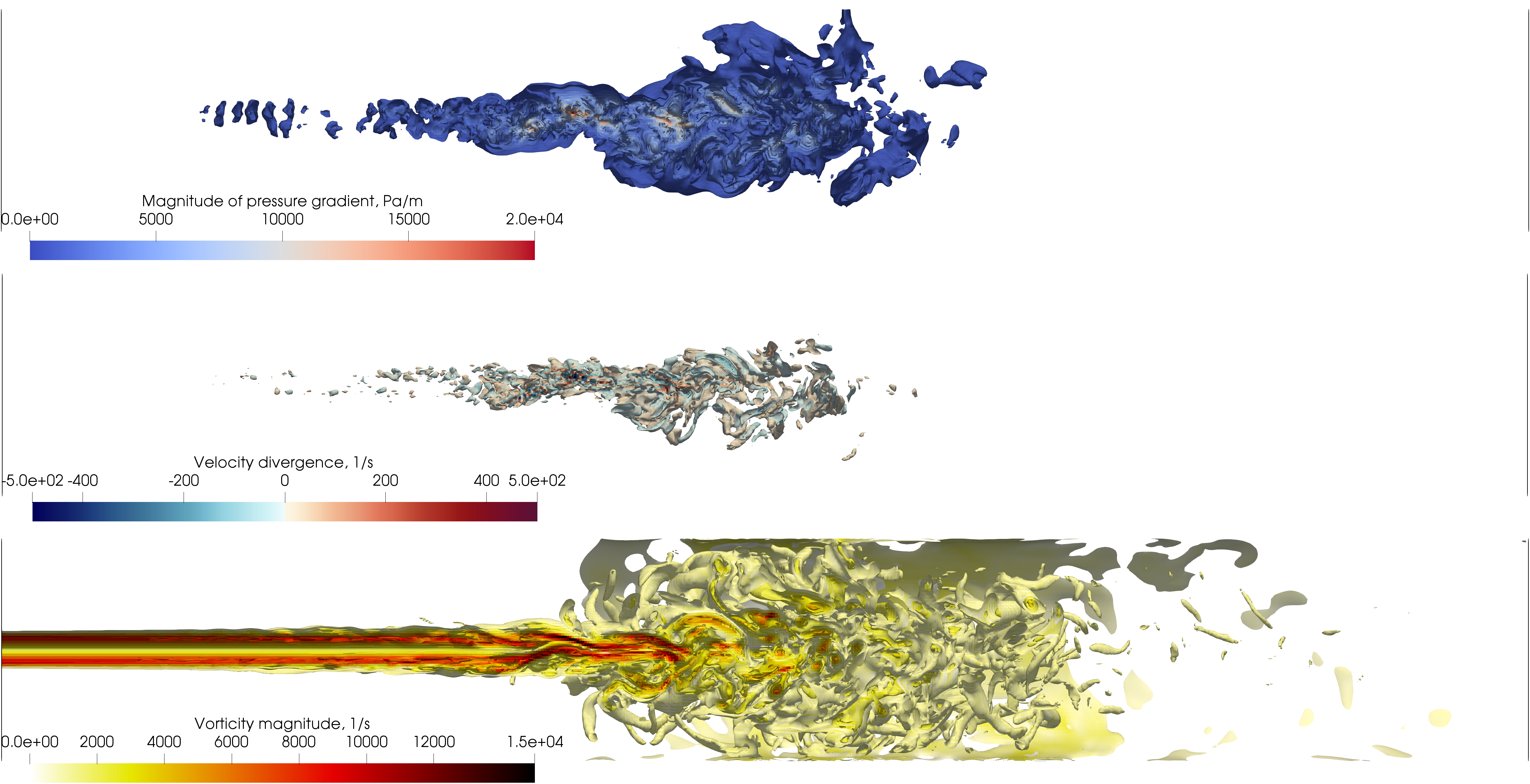
Figure 6. Magnitude of the pressure gradient (top), divergence of the velocity (middle) and magnitude of the vorticity (bottom) at time $t=0.15$ s.

For the divergence of velocity, observe that while its total scale is between $\pm 500$ s^-1, such extremal values manifest only in a few localized spots (just as for the pressure gradient above), whereas most values remain within $\pm 50$ s^-1, according to the colors of the level surfaces. The average value of $|\nabla\cdot\boldsymbol{u}|$ over the domain is

(4.3) $$\frac{1}{V}\int_{D}|\nabla\cdot\boldsymbol{u}|\>\!\mathrm{d}\boldsymbol{x}=0.932\text{ s}^{-1}.$$

In non-dimensional units, we have to multiply the result by $L/U\approx 3\cdot 10^{-4}$ s, which yields $\tilde{\nabla}\cdot\boldsymbol{\tilde{u}}\sim\pm 1.5\cdot 10^{-2}$, while the non-dimensional domain average of its absolute value is $\sim 3.2\cdot 10^{-4}$. These magnitudes are generally in agreement with $O(\mathit{Ma}^{2})\sim 10^{-2}$, as intended.

By contrast, the norm of vorticity is about two orders of magnitude larger than that of divergence throughout most of the domain; in particular, its domain average is

(4.4) $$\frac{1}{V}\int_{D}\|\nabla\times\boldsymbol{u}\|\>\!\mathrm{d}\boldsymbol{x}=408\text{ s}^{-1}.$$

This indicates that the overall structure of the flow is weakly compressible, and largely rotational.

In our recent works [25, 26, 27] we found that, in an inertial flow, the density and temperature variables could develop small scale fluctuations of as much as $\pm 60$% of their background values, which, of course, is unrealistic for low Mach number flows at normal conditions. We speculated that this happens because, in a realistic flow, the pressure gradient responds to large density and temperature fluctuations (thus allowing the flow to “compensate” for the latter), whereas in inertial flow the pressure gradient is zero.

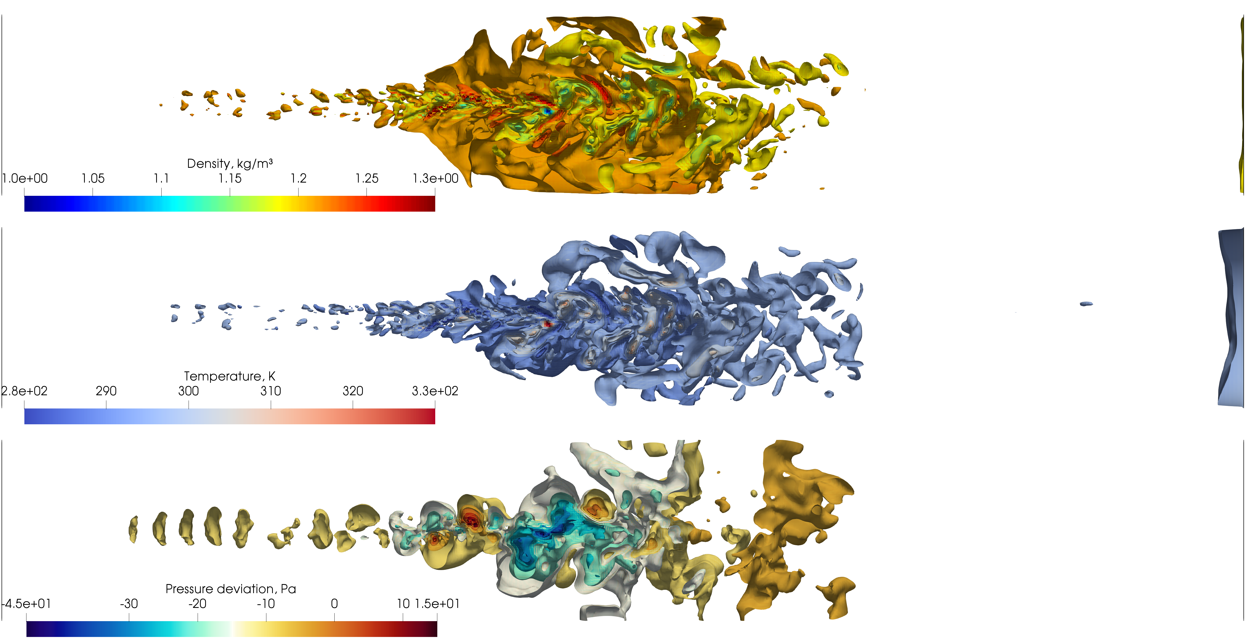
Figure 7. Density (top), temperature (middle) and pressure deviation (bottom) at time $t=0.15$ s.

Since in the weakly compressible model (2.24) the pressure is no longer constant, here we examine whether this modification has a beneficial effect on the density and temperature fluctuations. In Figure 7 we show the snapshots of density, temperature and the deviation of pressure from its background state of 101.3 kPa, produced in the same fashion as those of divergence and vorticity above. First, we note that the pressure deviations lie, at the extreme, between $-45$ Pa and $+15$ Pa; given the background state of $101.3$ kPa, this constitutes $-0.045$% and $+0.015$%, respectively, which indicates that the flow is still “almost” inertial. Yet, we can observe vast improvement in the fluctuations of density and temperature of the flow. For example, temperature now varies between $280$ K and $330$ K at the extreme (which for the background state of $293.15$ K constitutes only $-4.5$% and $+13$%, respectively) and even then, these extreme deviations are observed only at a few localized spots, while the majority of deviations are within the range of several degrees K. Moreover, the domain average of the temperature deviation from its background state of 293.15 K is

(4.5) $$\frac{1}{V}\int_{D}|T-293.15|\>\!\mathrm{d}\boldsymbol{x}=0.716\text{ K},$$

which constitutes 0.24% of the background state itself. A similar trend is observed for the density fluctuations. We conclude that the weakly compressible model in (2.24) produces notably more realistic behavior of density and temperature, than the inertial flow model in our recent works, while retaining the essential turbulent dynamics of the flow.

In addition to the snapshots of various properties of the flow, displayed above, we compute time averages of Fourier spectra of the streamwise kinetic energy. Each time average is computed in the same fashion as in our recent works [25, 26, 27, 28], within a cuboid region of 24 cm in length, and of 1$\times$1 cm² in cross-section. Six of these regions were placed inside the pipe, with their axes coinciding with the axis of the pipe, at 0, 4, 8, 16, 20 and 24 cm offsets from the inlet (such that the first region started at the inlet, while the sixth one ended at the outlet). In each region, the Fourier spectrum of the kinetic energy was computed as follows: first, the kinetic energy of the $x$-component of velocity, $E_{x}=u_{x}^{2}/2$, was averaged over the cross-section of the region, thus becoming the function of the $x$-coordinate only. Then, the linear trend was subtracted from the result in the same manner as was done by Nastrom and Gage [42] and also in our recent works [25, 26, 27, 28], to ensure that there was no sharp discontinuity between the energy values at the boundaries of the region. Finally, the one-dimensional discrete Fourier transformation was applied to the result. The subsequent time-averaging of the modulus of the Fourier transform was computed in the time interval $0.15\leq t\leq 0.25$ seconds of the elapsed model time.

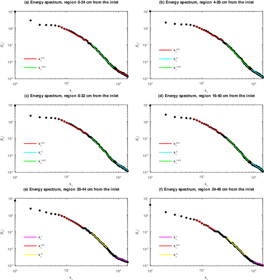
Figure 8. The Fourier spectra of the kinetic energy, computed within different regions, situated at (a) 0–24, (b) 4–28, (c) 8–32, (d) 16–40, (e) 20–44 and (f) 24–48 cm, counting from the inlet. The slope lines $k_{x}^{-1}$, $k_{x}^{-5/3}$, $k_{x}^{-2}$, $k_{x}^{-3}$ and $k_{x}^{-10/3}$ are given for reference.

We show the time averages of the kinetic energy spectra in Figure 8. Observe that, like in our recent works [25, 26, 27, 28], these spectra generally retain a power scaling structure. However, unlike our previous results (in particular, [27]), this structure appears to be somewhat different from what we observed before. While the Kolmogorov scaling $k_{x}^{-5/3}$ is still present at moderate scales (for $k_{x}$ roughly between 8 and 25), observe that at small scales ($k_{x}$ between 30 and 80) the slope of the plot corresponds to $k_{x}^{-10/3}$ for the first four regions, and to $k_{x}^{-3}$ for the last two regions. Additionally, at very small scales ($k_{x}>100$) the power scaling varies between $k_{x}^{-2}$ and $k_{x}^{-1}$, which has not been observed in our previous works. Additionally, Kolmogorov’s $k_{x}^{-5/3}$ scaling at moderate scales is present in all measurement regions, whereas in our recent work [27] it disappeared in the regions which approached the outlet. Given that the only difference between the weakly compressible system in (2.24) and the fully inertial flow in [25, 26, 27, 28] is a different treatment of the pressure variable, we have to conclude that the power structure of the kinetic energy spectrum is rather sensitive to the behavior of the pressure variable (recall from Figure 7 that pressure fluctuations constitute only a tiny fraction of its background value).

5. Summary

In the current work, we propose a new approach for treating the pressure variable, which we refer to as weakly compressible flow. Instead of setting the pressure so as to preserve the divergence of velocity along the streamline (as is done for incompressible flow), we instead formulate the pressure equation so that the divergence is linearly damped towards zero at an appropriate time rate. Our new approach is a compromise between compressible, incompressible and inertial flows, in the sense that it controls the pressure gradient at low Mach number, while simultaneously allowing the flow to be compressible, and has a more realistic density and temperature behavior than inertial flow. We find that, in the presence of the mean field effect of the intermolecular potential, our new model of weakly compressible flow spontaneously develops turbulent motions and power structures in its kinetic energy spectra, just like the inertial flow model did in our recent works [25, 26, 27, 28].

The results of the current work are rather encouraging. Clearly, our main finding here is that the spontaneous development of turbulence via the mean field effect of the intermolecular potential is robust under different treatments of the pressure variable; indeed, turbulence reliably develops in the same realistic fashion irrespectively of whether the flow is inertial (which usually happens at large scales, such as planetary scales) or weakly compressible (which is more realistic at small scales). This is in agreement with experiments and observations, where turbulent motions manifest similarly across a broad range of spatial scales, from centimeters to thousands of kilometers. This is also in sharp contrast with the conventional equations of fluid mechanics, both compressible and incompressible, where the spontaneous development of turbulence has not ever been observed despite overwhelming research efforts spanning more than a century.

The next step in this direction would be the development of an appropriate pressure model from fundamental physical principles, rather than technical considerations. Observe that, in the current work, the pressure treatment is “engineered”, rather than derived – the main argument is that we need to somehow keep the pressure gradient under control at low Mach number, and the proposed model is artificially tailored for that purpose. While at the current stage it is nevertheless a good result (at least in the particular case studied here), a systematic treatment of pressure, grounded in physical foundation, is essential for our turbulence model to provide reliable predictions in a broad range of real-world scenarios.

Acknowledgment

This work was supported by the Simons Foundation grant #636144.

References

- Boussinesq [1877] J. Boussinesq. Essai sur la théorie des eaux courantes. Mémoires présentés par divers savants à l’Académie des Sciences, XXIII(1):1–680, 1877.
- Reynolds [1883] O. Reynolds. An experimental investigation of the circumstances which determine whether the motion of water shall be direct or sinuous, and of the law of resistance in parallel channels. Proc. R. Soc. Lond., 35(224–226):84–99, 1883.
- Kolmogorov [1941a] A.N. Kolmogorov. Local structure of turbulence in an incompressible fluid at very high Reynolds numbers. Dokl. Akad. Nauk SSSR, 30:299–303, 1941a.
- Kolmogorov [1941b] A.N. Kolmogorov. Decay of isotropic turbulence in an incompressible viscous fluid. Dokl. Akad. Nauk SSSR, 31:538–541, 1941b.
- Kolmogorov [1941c] A.N. Kolmogorov. Energy dissipation in locally isotropic turbulence. Dokl. Akad. Nauk SSSR, 32:19–21, 1941c.
- Obukhov [1941] A.M. Obukhov. On the distribution of energy in the spectrum of a turbulent flow. Izv. Akad. Nauk SSSR Ser. Geogr. Geofiz., 5:453–466, 1941.
- Richardson [1926] L.F. Richardson. Atmospheric diffusion shown on a distance-neighbour graph. Proc. Roy. Soc. London A, 110:709–737, 1926.
- Taylor [1935] G.I. Taylor. Statistical theory of turbulence. Proc. Roy. Soc. London A, 151(873):421–444, 1935.
- Taylor [1938] G.I. Taylor. The spectrum of turbulence. Proc. Roy. Soc. London A, 164:476–490, 1938.
- de Kármán and Howarth [1938] T. de Kármán and L. Howarth. On the statistical theory of isotropic turbulence. Proc. Roy. Soc. London A, 164:192–215, 1938.
- Prandtl [1938] L. Prandtl. Beitrag zum Turbulenzsymposium. In J.P. Den Hartog and H. Peters, editors, Proceedings of the Fifth International Congress on Applied Mechanics, pages 340–346, Cambridge MA, 1938. John Wiley, New York.
- Obukhov [1949] A.M. Obukhov. Structure of the temperature field in turbulent flow. Izv. Akad. Nauk SSSR Ser. Geogr. Geofiz., 13:58–69, 1949.
- Chandrasekhar [1949] S. Chandrasekhar. On Heisenberg’s elementary theory of turbulence. Proc. Roy. Soc., 200:20–33, 1949.
- Corrsin [1951] S. Corrsin. On the spectrum of isotropic temperature fluctuations in an isotropic turbulence. J. Appl. Phys., 22(4):469–473, 1951.
- Kolmogorov [1962] A.N. Kolmogorov. A refinement of previous hypotheses concerning the local structure of turbulence in a viscous incompressible fluid at high Reynolds number. J. Fluid Mech., 13(1):82–85, 1962.
- Obukhov [1962] A.M. Obukhov. Some specific features of atmospheric turbulence. J. Geophys. Res., 67(8):3011–3014, 1962.
- Kraichnan [1966a] R.H. Kraichnan. Isotropic turbulence and inertial range structure. Phys. Fluids, 9:1728–1752, 1966a.
- Kraichnan [1966b] R.H. Kraichnan. Dispersion of particle pairs in homogeneous turbulence. Phys. Fluids, 9:1937–1943, 1966b.
- Saffman [1967] P.G. Saffman. The large-scale structure of homogeneous turbulence. J. Fluid Mech., 27(3):581–593, 1967.
- Saffman [1970] P.G. Saffman. A model for inhomogeneous turbulent flow. Proc. Roy. Soc. London A, 317:417–433, 1970.
- Mandelbrot [1974] B.B. Mandelbrot. Intermittent turbulence in self-similar cascades; divergence of high moments and dimension of the carrier. J. Fluid Mech., 62(2):331–358, 1974.
- Avila et al. [2011] K. Avila, D. Moxey, A. de Lozar, M. Avila, D. Barkley, and B. Hof. The onset of turbulence in pipe flow. Science, 333:192–196, 2011.
- Barkley et al. [2015] D. Barkley, B. Song, V. Mukund, G. Lemoult, M. Avila, and B. Hof. The rise of fully turbulent flow. Nature, 526:550–553, 2015.
- Khan et al. [2021] H.H. Khan, S.F. Anwer, N. Hasan, and S. Sanghi. Laminar to turbulent transition in a finite length square duct subjected to inlet disturbance. Phys. Fluids, 33:065128, 2021.
- Abramov [2021a] R.V. Abramov. Macroscopic turbulent flow via hard sphere potential. AIP Adv., 11(8):085210, 2021a.
- Abramov [2021b] R.V. Abramov. Turbulence in large-scale two-dimensional balanced hard sphere gas flow. Atmosphere, 12(11):1520, 2021b.
- Abramov [2022a] R.V. Abramov. Creation of turbulence in polyatomic gas flow via an intermolecular potential. Phys. Rev. Fluids, 7(5):054605, 2022a.
- Abramov [2022b] R.V. Abramov. Turbulence via intermolecular potential: Viscosity and transition range of the Reynolds number. Preprint: https://arxiv.org/abs/2202.04624, 2022b.
- Grad [1949] H. Grad. On the kinetic theory of rarefied gases. Comm. Pure Appl. Math., 2(4):331–407, 1949.
- Tsugé [1974] S. Tsugé. Approach to the origin of turbulence on the basis of two-point kinetic theory. Phys. Fluids, 17(1):22–33, 1974.
- Abramov [2020] R.V. Abramov. Turbulent energy spectrum via an interaction potential. J. Nonlinear Sci., 30:3057–3087, 2020.
- Lennard-Jones [1924] J.E. Lennard-Jones. On the determination of molecular fields. – II. From the equation of state of a gas. Proc. R. Soc. Lond. A, 106(738):463–477, 1924.
- Boublík [2006] T. Boublík. Hard-sphere radial distribution function from the residual chemical potential. Mol. Phys., 104(22–24):3425–3433, 2006.
- Cercignani et al. [1994] C. Cercignani, R. Illner, and M. Pulvirenti. The mathematical theory of dilute gases. In Applied Mathematical Sciences, volume 106. Springer-Verlag, 1994.
- Hirschfelder et al. [1964] J.O. Hirschfelder, C.F. Curtiss, and R.B. Bird. The Molecular Theory of Gases and Liquids. Wiley, 1964.
- Batchelor [2000] G.K. Batchelor. An Introduction to Fluid Dynamics. Cambridge University Press, New York, 2000.
- Golse [2005] F. Golse. The Boltzmann Equation and its Hydrodynamic Limits, volume 2 of Handbook of Differential Equations: Evolutionary Equations, chapter 3, pages 159–301. Elsevier, 2005.
- Weller et al. [1998] H.G. Weller, G. Tabor, H. Jasak, and C. Fureby. A tensorial approach to computational continuum mechanics using object-oriented techniques. Computers in Physics, 12(6):620–631, 1998.
- van Leer [1974] B. van Leer. Towards the ultimate conservative difference scheme, II: Monotonicity and conservation combined in a second order scheme. J. Comput. Phys., 17:361–370, 1974.
- Issa [1986] R.I. Issa. Solution of the implicitly discretised fluid flow equations by operator-splitting. J. Comput. Phys., 62(1):40–65, 1986.
- Buchhave and Velte [2017] P. Buchhave and C.M. Velte. Measurement of turbulent spatial structure and kinetic energy spectrum by exact temporal-to-spatial mapping. Phys. Fluids, 29(8):085109, 2017.
- Nastrom and Gage [1985] G.D. Nastrom and K.S. Gage. A climatology of atmospheric wavenumber spectra of wind and temperature observed by commercial aircraft. J. Atmos. Sci., 42(9):950–960, 1985.