On Efficient Online Imitation Learning
via Classification

Abstract

Imitation learning (IL) is a general learning paradigm for tackling sequential decision-making problems. Interactive imitation learning, where learners can interactively query for expert demonstrations, has been shown to achieve provably superior sample efficiency guarantees compared with its offline counterpart or reinforcement learning. In this work, we study classification-based online imitation learning (abbrev. COIL) and the fundamental feasibility to design oracle-efficient regret-minimization algorithms in this setting, with a focus on the general nonrealizable case. We make the following contributions: (1) we show that in the COIL problem, any proper online learning algorithm cannot guarantee a sublinear regret in general; (2) we propose Logger, an improper online learning algorithmic framework, that reduces COIL to online linear optimization, by utilizing a new definition of mixed policy class; (3) we design two oracle-efficient algorithms within the Logger framework that enjoy different sample and interaction round complexity tradeoffs, and conduct finite-sample analyses to show their improvements over naive behavior cloning; (4) we show that under the standard complexity-theoretic assumptions, efficient dynamic regret minimization is infeasible in the Logger framework. Our work puts classification-based online imitation learning, an important IL setup, into a firmer foundation.

1 Introduction

Imitation learning (IL), also known as learning from expert demonstrations pomerleau1988alvinn ; osa2018algorithmic , is a general paradigm for training intelligent behavior for sequential decision making tasks. IL has been successfully deployed in many applications, such as autonomous driving pomerleau1988alvinn ; pan2020imitation , robot arm control wang2017robust , game playing silver2016mastering , and sequence prediction daume2009search ; bengio2015scheduled . It is now well-known that with the help of a demonstrating expert, an IL agent can bypass the exploration challenges of reinforcement learning, achieving a much lower sample requirement than reinforcement learning agents sun2017deeply .

Two major IL paradigms have been studied in the literature: offline and interactive. In offline IL abbeel2004apprenticeship ; syed2007game ; ziebart2008maximum ; ho2016generative , the learner receives a set of expert demonstrations ahead of time; in contrast, in interactive IL daume2009search ; ross2011reduction ; ross2014reinforcement ; judah2014active , the learner has the ability to interactively query the expert for demonstrations on states at its disposal, allowing expert feedback to be provided in a targeted manner. In both settings, the goal of the learner is to output a policy $\hat{\pi}$ that competes with the expert’s policy $\pi^{E}$, by consuming as few resources (e.g. expert annotations) as possible. Between these two, interactive IL is known to be able to achieve superior policy performance than its offline counterpart under certain favorable assumptions on the expert policy and the environment, in that learning agents can use interaction to address the compounding error challenge ross2010efficient ; rajaraman2021value .

Despite the recent progress in the fundamental limits of the interactive imitation learning in the realizable setting sun2017deeply ; rajaraman2020toward ; rajaraman2021value , the statistical and computational limits of the interactive imitation learning in the general nonrealizable setting remain open. One promising and influential algorithmic framework for studying and analyzing interactive IL in the nonrealizable setting is DAgger (Data Aggregation) ross2011reduction , whose key insight is to reduce interactive IL to regret minimization in online learning shalev2011online . Specifically, it constructs a $N$-round online learning game, where at every round $n\in[N]$, the learner outputs some policy $\pi_{n}$ from a policy class $\mathcal{B}$, and incurs a loss $F_{n}(\pi)$; the loss is carefully constructed so that the learner’s instantaneous loss $F_{n}(\pi_{n})$ characterizes current policy $\pi_{n}$’s competitiveness compared to the expert $\pi^{E}$. A representative example of $F_{n}(\pi)$ is the expected disagreement between $\pi$ and $\pi^{E}$ on the state occupancy distribution induced by $\pi_{n}$, used in the original DAgger paper ross2011reduction , which can be expressed as the expected zero-one loss of $\pi$ on a distribution of classification examples – we call such setting Classification-based Online Imitation Learning (abbrev. COIL). The DAgger reduction framework has spurred an active line of research on IL ross2014reinforcement ; sun2017deeply ; cheng2018convergence ; cheng2019accelerating ; cheng2019predictor ; lee2021dynamic : it enables conversions from stochastic online optimization algorithms with static or dynamic regret guarantees to IL algorithms with different output policy suboptimality guarantees, allowing the research community to directly translate new results in online learning to the field of IL.

Perhaps surprisingly, from a fundamental perspective, rigorous design of efficient regret minimization algorithms for COIL has been largely overlooked by the prior literature. Specifically, many works assume a fixed parameterization of policies in $\mathcal{B}$, and assume that $F_{n}(\pi)$’s are convex in $\pi$’s underlying parameters to allow for no-regret online convex optimization ross2011reduction ; sun2017deeply ; cheng2018convergence . Although natural, this viewpoint has two issues: (1) in DAgger’s reduction, the learner uses finite-sample approximations of $F_{n}(\pi)$, which are often discontinuous in $\pi$’s underlying parameters (e.g. given a policy $\pi_{\theta}(s)=\mathrm{sign}(\left\langle\theta,s\right\rangle)$ as a linear classifier, its zero-one loss on a state, $I(\pi_{\theta}(s)\neq\pi^{E}(s))$ is discontinuous in $\theta$), making stochastic gradient-based methods inapplicable. Convex surrogate loss functions has been proposed as a popular workaround ross2011reduction , but it is well-known that in the nonrealizable setting, even for the special case of supervised learning, minimizing convex surrogate losses can result in very different models compared to minimizing the original zero-one classification loss ben2012minimizing ; (2) it makes the usage of policy classes with complex parameterization (e.g. rule-based policies such as decision trees) difficult, as convexity is hard to establish for such classes.

An overview of our results.

In this paper, we bridge the above-mentioned gaps by studying the fundamental feasibility of designing efficient regret minimization algorithms for COIL, putting the study of statistical and computational limits of interactive imitation learning in the general nonrealizable setting into a firmer foundation. Our first result is that, analogous to Cover’s impossibility result in online classification cover1966behavior , in the COIL setting, any proper online learning algorithm (that outputs a sequence of policies $\{\pi_{n}\}_{n=1}^{N}$ from the original class $\mathcal{B}$) cannot guarantee sublinear regret in general (§ 3.1).

The above negative result motivates the design of improper learning algorithms for regret minimization. To this end, we propose to choose policies from a mixed policy class $\Pi_{\mathcal{B}}$, and provide an algorithmic framework, Logger, that reduces COIL to online linear optimization. In a nutshell, Logger uses a natural parameterization on $\Pi_{\mathcal{B}}$ that allows to express $F_{n}(\pi)$ as a linear function of the underyling parameters of $\pi\in\Pi_{\mathcal{B}}$. We show that any online linear optimization algorithm with (high-probability) regret guarantees can be plugged into Logger to obtain an algorithm for COIL with policy suboptimality guarantees (§ 3.2).

Next, enabled by the Logger framework, we design computationally efficient algorithms for static regret minimization. Assuming access to an offline cost-sensitive classification (CSC) oracle $\mathcal{O}$, and a set of unlabeled separator examples for $\mathcal{B}$ syrgkanis2016efficient ; dudik2020oracle , we design Logger-M, a sample and computationally efficient algorithm. Using $O(1/\epsilon^{2})$ interaction rounds and $O(1/\epsilon^{2})$ expert annotations, Logger-M enjoys a per-round static regret of $\epsilon$ (§ 4.1). Underlying Logger-M is a delicate utilization of the connection between Follow-the-Perturbed-Leader and Follow-the-Regularized-Leader, two well-known online learning algorithm families, first observed by abernethy2014online . Moreover, by exploiting the predictability of the COIL problem rakhlin2013online ; cheng2019accelerating ; cheng2019predictor , we design an efficient algorithm Logger-ME, that enjoys a per-round static regret of $\epsilon$, with $O(1/\epsilon)$ interaction rounds and $O(1/\epsilon^{2})$ expert annotations (§ 4.2). Its reduced number of interaction rounds can enable a more practical deployment of IL agents, especially when interactive expert annotations come in batches or with delays.

Finally, we study efficient dynamic regret minimization in the Logger framework (§ 5). We show that this is unlikely to be feasible: under a standard complexity-theoretic assumption, no oracle-efficient algorithms can output policies in $\Pi_{\mathcal{B}}$ with sublinear dynamic regret. Due to space constraints, we discuss key related works throughout the paper, and defer additional related works to Appendix A.

2 Preliminaries

Basic definitions.

Define $[n]\mathrel{\mathop{\mathchar 58\relax}}=\mathinner{\left\{1,\ldots,n\right\}}$. Define indicator function $I(\cdot)$ such that $I(E)=1$ if condition $E$ is true, and $=0$ otherwise. We use $\Delta(W)$ to denote the set of probability distributions over a finite set $W$, and use $\operatorname{Onehot}(w,W)\in\Delta(W)$ to denote the delta mass on $w\in W$. For a finite $W$, we will oftentimes treat $u\in\mathbb{R}^{|W|}$ (e.g. $u\in\Delta(W)$) as a $\left|W\right|$-dimensional vector; for $w\in W$, denote by $u[w]$ the $w$-th coordinate of $u$. We abuse the notation of $\{\cdot\}$ to denote multisets.

Episodic MDPs.

We study imitation learning in episodic Markov decision processes (MDPs). An episodic MDP $\mathcal{M}$ is a tuple $({\mathcal{S}},\mathcal{A},H,c,\rho,P)$, where ${\mathcal{S}}$ is a finite state space (that can be exponentially large), $\mathcal{A}$ is a finite action set, $H\in\mathbb{N}^{+}$ is the episode length, $c\mathrel{\mathop{\mathchar 58\relax}}{\mathcal{S}}\times\mathcal{A}\rightarrow[0,1]$ is the cost function, and $\rho\in\Delta({\mathcal{S}})$ is the initial state distribution. Also, $P=\{P_{t}\}_{t=1}^{H-1}$ denotes $\mathcal{M}$’s transition dynamics, with $P_{t}\mathrel{\mathop{\mathchar 58\relax}}{\mathcal{S}}\times\mathcal{A}\to\Delta({\mathcal{S}})$ being the transition probability at step $t$. Throughout, we use $S$ and $A$ to denote $|{\mathcal{S}}|$ and $|\mathcal{A}|$, respectively. Without loss of generality, we assume that $\mathcal{M}$ is layered, where ${\mathcal{S}}$ can be partitioned into $H$ disjoint sets $\{{\mathcal{S}}_{t}\}_{t=1}^{H}$; the initial distribution $\rho$ is supported on ${\mathcal{S}}_{1}$, and transition distribution $P_{t}(\cdot\mid s,a)$ is supported on ${\mathcal{S}}_{t+1}$ for all $t,s,a$. For state $s\in{\mathcal{S}}$, define $\mathrm{Step}(s)$ as the step $t$ such that $s\in{\mathcal{S}}_{t}$.

A learning agent interacts with $\mathcal{M}$ for one episode using the following protocol: for every step $t\in[H]$: it observes a state $s_{t}\in{\mathcal{S}}_{t}$, takes an action $a_{t}\in\mathcal{A}$, incurs cost $c(s_{t},a_{t})$, and transitions to next state $s_{t+1}\sim P_{t}(\cdot\mid s_{t},a_{t})$ except for the last step when it stops. Given a stationary policy $\pi\mathrel{\mathop{\mathchar 58\relax}}{\mathcal{S}}\rightarrow\Delta(\mathcal{A})$, we use $\pi(\cdot|s)$ to denote the action distribution of $\pi$ on $s$. Denote by $\mathbb{E}_{\pi}$ and $\mathbb{P}_{\pi}$ the expectation and probability over executing (i.e. rolling out) policy $\pi$ in $\mathcal{M}$. Given policy $\pi$, its state occupancy distribution at step $t$ is defined as $d_{\pi}^{t}(\cdot)\mathrel{\mathop{\mathchar 58\relax}}=\mathbb{P}_{\pi}(s_{t}=\cdot)$; its average state occupancy distribution is denoted as $d_{\pi}\mathrel{\mathop{\mathchar 58\relax}}=\frac{1}{H}\sum_{t=1}^{H}d_{\pi}^{t}$. Let $J(\pi)\mathrel{\mathop{\mathchar 58\relax}}=\mathbb{E}_{\pi}\left[\sum_{t=1}^{H}c(s_{t},a_{t})\right]=H\cdot\mathbb{E}_{s\sim d_{\pi}}\mathbb{E}_{a\sim\pi(\cdot|s)}\left[c(s,a)\right]$ denote the expected cumulative cost of $\pi$ over an episode. For policy $\pi$, we denote its value function $V_{\pi}(s)\mathrel{\mathop{\mathchar 58\relax}}=\mathbb{E}\left[\sum_{t=\mathrm{Step}(s)}^{H}c(s_{t},a_{t})\mid s,\pi\right]$ and action-value function $Q_{\pi}(s,a)\mathrel{\mathop{\mathchar 58\relax}}=c(s,a)+\mathbb{E}\left[\sum_{t=\mathrm{Step}(s)+1}^{H}c(s_{t},a_{t})\mid s,a,\pi\right]$; in words, they are the expected costs of rolling out $\pi$ starting from $s$ and $(s,a)$, respectively. For policy $\pi$, define its advantage function as $A_{\pi}(s,a)\mathrel{\mathop{\mathchar 58\relax}}=Q_{\pi}(s,a)-V_{\pi}(s)$, which measures the expected performance difference by one step deviation of $\pi$ by taking action $a$ at state $s$. Also, we define the recoverability constant as the ability of $\pi$ to recover from deviation when rolled out in $\mathcal{M}$:

Definition 1 ($\mu$-recoverability).

A (MDP, policy) pair $(\mathcal{M},\pi)$ is said to be $\mu$-recoverable, if $\forall s\in{\mathcal{S}},a\in\mathcal{A}$, $\left|A_{\pi}(s,a)\right|\leq\mu$. 

Interactive IL.

We study interactive imitation learning daume2009search ; ross2010efficient , where the learner has access to a stationary deterministic demonstrating expert $\pi^{E}$ and would like to learn a policy with low expected cost. Throughout, we assume that $(\mathcal{M},\pi^{E})$ is $\mu$-recoverable, for some $\mu\leq H$ that can potentially be $\ll H$. At each interaction round, the learner interacts with $\mathcal{M}$ for a few episodes, obtaining trajectories of the form $\tau=(s_{1},a_{1},s_{2},a_{2},\ldots,s_{H},a_{H})$ and queries the expert for feedback on some of the states. Specifically, given a state $s$, the feedback given by the expert is of the form $(\zeta_{E}(s,a))_{a\in\mathcal{A}}\in\mathbb{R}^{A}$. Two notable examples are: (1) direct expert annotation ross2011reduction , i.e. given state $s$, expert provides demonstration $\pi^{E}(s)$, and we use it to construct an $A$-dimensional feedback $(\zeta_{E}(s,a))_{a\in\mathcal{A}}=(\mu\cdot I(a\neq\pi^{E}(s)))_{a\in\mathcal{A}}$; (2) estimates of value functions based on experts’ rollout ross2014reinforcement , i.e. $(\zeta_{E}(s,a))_{a\in\mathcal{A}}=(A^{E}(s,a))_{a\in\mathcal{A}}\mathrel{\mathop{\mathchar 58\relax}}=(A_{\pi^{E}}(s,a))_{a\in\mathcal{A}}$. Throughout, we assume $\zeta_{E}(s,a)$ satisfies $\forall s\in{\mathcal{S}},a\in\mathcal{A}$, $A^{E}(s,a)\leq\zeta_{E}(s,a)\leq\mu\cdot I(a\neq\pi^{E}(s))$; this is satisfied by the two examples above. Define a policy $\pi$’s imitation loss as: $L(\pi)\mathrel{\mathop{\mathchar 58\relax}}=\mathbb{E}_{s\sim d_{\pi}}\mathbb{E}_{a\sim\pi(\cdot|s)}\left[\zeta_{E}(s,a)\right]$. By the performance difference lemma Kakade2002ApproximatelyOA (see Lemma 55 in Appendix H), $J(\pi)-J(\pi^{E})\leq H\cdot L(\pi)$, implying that if $\pi$ has a small imitation loss, it will have expected cost competitive with $\pi^{E}$. In light of this connection, in interactive IL, the learner would like to obtain policy $\hat{\pi}$ with low $L(\hat{\pi})$. Subject to this, throughout the paper, we consider the learner to optimize two measures of data efficiency:

• Sample complexity: the total number of expert annotations $\zeta_{E}$ requested. A smaller sample complexity reduces the total cost of expert annotations (which often takes human effort).

• Interaction round complexity: total number of adaptive interaction rounds. A small number of interaction rounds enables more parallelized annotations within an interaction round, and mitigates the delayed annotation issue yang2013buy ; wang2021one .

The DAgger reduction framework for interactive IL.

The DAgger framework reduces minimizing $L(\pi)$ to no-regret online learning ross2011reduction ; ross2014reinforcement . It constructs a $N$-round online learning game, where at every round $n\in[N]$, the learner outputs some policy $\pi_{n}$, which induces a loss function $F_{n}(\pi)=\mathbb{E}_{s\sim d_{\pi_{n}}}\mathbb{E}_{a\sim\pi(\cdot|s)}\left[\zeta_{E}(s,a)\right]$ . Its key insight is that, by the definition of $\mathinner{\left\{F_{n}\right\}}_{n=1}^{N}$, minimizing the online learning cumulative loss $\sum_{n=1}^{N}F_{n}(\pi_{n})$ is equivalent to minimizing the cumulative imitation losses of $\pi_{n}$’s, i.e. $\sum_{n=1}^{N}L(\pi_{n})$. Research efforts in online learning shalev2011online have focused on the design of algorithms that can output $\mathinner{\left\{\pi_{n}\right\}}_{n=1}^{N}$ with static regret $\mathrm{SReg}_{N}(\mathcal{B})$ or dynamic regret $\mathrm{DReg}_{N}(\mathcal{B})$ against some benchmark policy class $\mathcal{B}$, formally:

$$\mathrm{SReg}_{N}(\mathcal{B})\mathrel{\mathop{\mathchar 58\relax}}=\sum_{n=1}^{N}F_{n}(\pi_{n})-\min_{\pi\in\mathcal{B}}\sum_{n=1}^{N}F_{n}(\pi),\quad\mathrm{DReg}_{N}(\mathcal{B})\mathrel{\mathop{\mathchar 58\relax}}=\sum_{n=1}^{N}\left(F_{n}(\pi_{n})-\min_{\pi\in\mathcal{B}}F_{n}(\pi)\right).$$ (1)

Protocol 1 Classification-based Online Imitation Learning (COIL)

  for $n=1,\ldots,N$ do

     Learner outputs policy $\pi_{n}$.

     Loss function $F_{n}(\pi)\mathrel{\mathop{\mathchar 58\relax}}=\mathbb{E}_{s\sim d_{\pi_{n}}}\mathbb{E}_{a\sim\pi(\cdot\mid s)}\left[\zeta_{E}(s,a)\right]$.

     Learner draws samples from $\mathcal{D}^{E}_{\pi_{n}}$ to obtain information about loss $F_{n}$, via interacting with $\mathcal{M}$ and querying the expert for annotation $\zeta_{E}$.

  end for

  Goal of learner: minimize $\sum_{n=1}^{N}F_{n}(\pi_{n})=\sum_{n=1}^{N}L(\pi_{n})$.

Assuming that the learner chooses policies $\mathinner{\left\{\pi_{n}\right\}}_{n=1}^{N}$ from another stationary policy class $\mathcal{B}_{0}$ (which may or may not be $\mathcal{B}$), the following proposition shows that static and dynamic regret guarantees in the induced online learning game can be converted to policy suboptimality guarantees:

Proposition 2 (e.g. cheng2018convergence ).

For any $N\in\mathbb{N}^{+}$ and online learner that outputs $\mathinner{\left\{\pi_{n}\right\}}_{n=1}^{N}\in\mathcal{B}_{0}^{N}$, define $\mathrm{Bias}(\mathcal{B},\mathcal{B}_{0},N)\mathrel{\mathop{\mathchar 58\relax}}=\mathop{\max}\limits_{\{\upsilon_{n}\}_{n=1}^{N}\in\mathcal{B}_{0}^{N}}\min\limits_{\pi\in\mathcal{B}}\mathbb{E}_{s\sim\bar{d}_{N}}\mathbb{E}_{a\sim\pi(\cdot\mid s)}\left[I(a\neq\pi^{E}(s))\right]$, where $\bar{d}_{N}\mathrel{\mathop{\mathchar 58\relax}}=\frac{1}{N}\sum_{n=1}^{N}d_{\upsilon_{n}}$. Then, choosing $\hat{\pi}$ uniformly at random from $\mathinner{\left\{\pi_{n}\right\}}_{n=1}^{N}$ has guarantee:

$$\mathbb{E}\left[J(\hat{\pi})-J(\pi^{E})\right]\leq H\cdot\min\mathinner{\left\{\mu\cdot\mathrm{Bias}(\mathcal{B},\mathcal{B}_{0},N)+\frac{\mathbb{E}[\mathrm{SReg}_{N}(\mathcal{B})]}{N},\;\mu\cdot\mathrm{Bias}(\mathcal{B},\mathcal{B}_{0},1)+\frac{\mathbb{E}[\mathrm{DReg}_{N}(\mathcal{B})]}{N}\right\}}.$$

In the above proposition, $\mathrm{Bias}(\mathcal{B},\mathcal{B}_{0},N)$ takes the worst-case mixture of state occupancy distributions $\mathinner{\left\{d_{\upsilon_{n}}\right\}}_{n=1}^{N}$ induced by $N$ policies from $\mathcal{B}_{0}$, and measures the expected disagreement between $\pi^{E}$ and its best approximating policy in $\mathcal{B}$. Informally, it measures the “approximation error” of benchmark class $\mathcal{B}$: it is always nonnegative, and when $\pi^{E}\in\mathcal{B}$ (which we call the realizable case), $\mathrm{Bias}(\mathcal{B},\mathcal{B}_{0},N)=0$. Proposition 2 gives two ways to obtain a competitive imitation policy: (1) choose $(\mathcal{B},\mathcal{B}_{0})$ with a small $\mathrm{Bias}(\mathcal{B},\mathcal{B}_{0},N)$ and achieve a low static regret; (2) choose $(\mathcal{B},\mathcal{B}_{0})$ with a small $\mathrm{Bias}(\mathcal{B},\mathcal{B}_{0},1)$ and achieve a low dynamic regret. Although achieving low dynamic regret can be significantly more challenging than achieving low static regret, minimizing dynamic regret has the advantage that its approximation error term $\mathrm{Bias}(\mathcal{B},\mathcal{B}_{0},1)$ is smaller than the static regret formulation’s counterpart $\mathrm{Bias}(\mathcal{B},\mathcal{B}_{0},N)$.

Classification-based Online Imitation Learning (COIL).

As we consider a finite action space $\mathcal{A}$, a policy $\pi$ can be equivalently viewed as a (possibly randomized) multiclass classifier. A cost-sensitive classification (CSC) example is defined to be a pair $(x,\vec{c})$, where $x\in{\mathcal{S}}$ is its feature part, and $\vec{c}\in\mathbb{R}^{A}$ is its cost part. Under the DAgger reduction framework, the loss at iteration $n$, $F_{n}(\pi)=\mathbb{E}_{s\sim d_{\pi_{n}}}\mathbb{E}_{a\sim\pi(\cdot|s)}\left[\zeta_{E}(s,a)\right]$, can be viewed as the expected cost of policy $\pi$ on a distribution of cost-sensitive examples $\mathcal{D}^{E}_{\pi_{n}}$ (formally, $\mathbb{E}_{(s,\vec{c})\sim\mathcal{D}^{E}_{\pi_{n}}}\left[\vec{c}(h(s))\right]$), where a sample $(s,\vec{c})$ is drawn from $\mathcal{D}^{E}_{\pi}$ by first rolling out $\pi$ and drawing $s\sim d_{\pi}$, and query the expert on $s$ to obtain $(\zeta_{E}(s,a))_{a\in\mathcal{A}}$ as its associated $\vec{c}$. The learner can obtain a finite-sample approximation to $F_{n}(\pi)$ by interacting with $\mathcal{M}$ and the expert to draw samples from $\mathcal{D}^{E}_{\pi_{n}}$. We will focus on designing efficient regret-minimizing algorithms in the COIL setting; see Protocol 1 for a summary.

In addition to data efficiency, we also consider the design of imitation learning algorithms with computational efficiency guarantees. To this end, following a sequence of empirically and theoretically successful works on oracle-efficient learning syrgkanis2016efficient ; dudik2011efficient ; agarwal2014taming ; dann2018oracle , we assume access to the benchmark policy class $\mathcal{B}$, which is a collection of $B$ stationary deterministic policies $h\mathrel{\mathop{\mathchar 58\relax}}{\mathcal{S}}\rightarrow\mathcal{A}$. Throughout this paper, we assume access to the following computational oracle for class $\mathcal{B}$ and measure an algorithm’s computational efficiency by its number of calls to this oracle.

Definition 3 (CSC oracle).

A CSC oracle $\mathcal{O}$ for policy class $\mathcal{B}$ is such that: given any input multiset of cost-sensitive examples $D=\{(x_{1},\vec{c}_{1}),\ldots,(x_{K},\vec{c}_{K})\}\in({\mathcal{S}}\times\mathbb{R}^{A})^{K}$, it outputs the policy in $\mathcal{B}$ that has the smallest empirical cost, formally,

$$\mathcal{O}(D)\mathrel{\mathop{\mathchar 58\relax}}=\mathop{\mathrm{argmin}}_{h\in\mathcal{B}}\mathbb{E}_{(x,\vec{c})\sim D}\left[\vec{c}(h(x))\right],$$

where we slightly abuse the notation and and use $D$ to also denote the uniform distribution over it.

3 Logger: reducing COIL to online linear optimization

In this section, we introduce our main algorithmic framework, Logger (an abbreviation for Linear lOss aGGrEgation) for designing regret-minimizing algorithms in the COIL setting. Section 3.1 motivates our approach by showing that natural proper learning-based approaches fail to achieve sublinear regret in general; Section 3.2 introduces the main idea of performing improper learning using a carefully-defined mixture policy class, via a reduction to online linear optimization.

3.1 Can we achieve sublinear regret using proper learning?

A natural idea for minimizing regret is proper learning: at round $n$, the learner chooses some policy $\pi_{n}$ (possibly at random) from $\mathcal{B}_{0}=\mathcal{B}$, our benchmark policy class, using some online learning algorithm, based on all information collected in the first $n-1$ rounds; the learner collects information on $F_{n}$ via rollouts of $\pi_{n}$ and expert annotations, and continue to the next iteration.

While this approach has demonstrated sharp online regret guarantees in classical online cost-sensitive classification settings littlestone1994weighted ; freund1997decision , perhaps subtly, we show in the following theorem that, this approach is insufficient to guarantee sublinear regret in the COIL setting.

Theorem 4.

Suppose the expert’s feedback $\zeta_{E}(s,a)$ is of the form $\mu\cdot I(a\neq\pi^{E}(s))$ or $A^{E}(s,a)$. Then, for any $H\geq 3$, there exists an MDP $\mathcal{M}$ of episode length $H$, a deterministic expert policy $\pi^{E}$, a benchmark policy class $\mathcal{B}$, such that for any learner that sequentially and possibly at random generates a sequence of policies $\{\pi_{n}\}_{n=1}^{N}\in\mathcal{B}^{N}$, its static regret satisfies $\mathrm{SReg}_{N}(\mathcal{B})=\Omega(N).$

The proof of the theorem can be found at Appendix D.1. Its key insight is that, distinct from the classical online CSC setting, in COIL, the loss at round $n$, $F_{n}$, depends on the policy chosen at that round $\pi_{n}$, making standard regret minimization results in online classification littlestone1994weighted ; freund1997decision inapplicable. In more detail, we construct MDPs that act “adversarially” to policies in $\mathcal{B}$, such that any $\pi_{n}\in\mathcal{B}$ has $F_{n}(\pi_{n})\geq\frac{N(H-1)}{H}$, whereas $\min_{\pi\in\mathcal{B}}\sum_{n}^{N}F_{n}(\pi)\leq\frac{N}{2}$. Our theorem is similar in spirit to Cover’s impossibility result in online classification cover1966behavior , which shows that an adversary that adapts to the randomness of the learner at each round can force the learner to suffer linear regret.

3.2 A new hypothesis class and the Logger algorithmic framework

To sidestep the impossibility result in Theorem 4, we apply the “convexification by randomization” technique in online convex optimization shalev2011online by improper learning on a mixed policy class, defined below.

Definition 5 (Mixed policy class).

Given policy class $\mathcal{B}$, define its induced mixed policy class

$$\Pi_{\mathcal{B}}\mathrel{\mathop{\mathchar 58\relax}}=\mathinner{\left\{\pi_{u}(\cdot|s)\mathrel{\mathop{\mathchar 58\relax}}=\sum_{h\in\mathcal{B}}u[h]\cdot h(\cdot|s)\mathrel{\mathop{\mathchar 58\relax}}u\in\Delta(\mathcal{B})\right\}}.$$

We slightly abuse notation and use $h(\cdot\mid s)\in\Delta(\mathcal{A})$ to denote the delta mass on $h(s)\in\mathcal{A}$.

Algorithm 2 Logger: reducing COIL to online linear optimization

1:  Input: MDP $\mathcal{M}$, Expert feedback $\zeta_{E}$, sample size per iteration $K$, Online linear optimization algorithm $\mathrm{OLOA}$ with decision set $\Delta(\mathcal{B})$.

2:  for $n=1,2,\ldots,N$ do

3:     Choose $u_{n}\leftarrow\mathrm{OLOA}(\{g_{i}\}_{i=1}^{n-1})$, which induces policy $\pi_{n}\mathrel{\mathop{\mathchar 58\relax}}=\pi_{u_{n}}$.

4:     Draw $K$ examples $D_{n}=\mathinner{\left\{(s,\vec{c})\right\}}$ iid from $\mathcal{D}^{E}_{\pi_{n}}$, via interaction with $\mathcal{M}$ and expert $\zeta_{E}$.

5:     $D_{n}$ induces $g_{n}=\left(\mathbb{E}_{(s,\vec{c})\sim D_{n}}\mathbb{E}_{a\sim h(\cdot\mid s)}\left[\vec{c}(a)\right]\right)_{h\in\mathcal{B}}$, an unbiased estimate of $\theta(u_{n})$.

6:  end for

At a cursory glance, choosing a policy from $\Pi_{\mathcal{B}}$ seems equivalent to choosing some policy at random from $\mathcal{B}$, which also falls into the failure mode of proper learning (Theorem 4). We remark that this is not true: rolling out a policy from $\pi_{u}\in\Pi_{\mathcal{B}}$ is equivalent to drawing new policies in the i.i.d. manner from $\mathcal{B}$ at every step of the episode instead. As we will see next, using $\Pi_{\mathcal{B}}$ enables the design of algorithms with sublinear regret.

The key observation is with the learner outputting policies from the mixed policy class $\Pi_{\mathcal{B}}$, online regret minimization in IL becomes an online linear optimization problem. Recall that in online IL, the loss at round $n$ is $F_{n}(\pi)=\mathbb{E}_{s\sim d_{\pi_{n}}}\mathbb{E}_{a\sim\pi(\cdot\mid s)}\left[\zeta_{E}(s,a)\right]$. By choosing $\pi_{n}=\pi_{u_{n}}\in\Pi_{\mathcal{B}}$ and $\pi=\pi_{u}\in\Pi_{\mathcal{B}}$ for $u_{n},u\in\Delta(\mathcal{B})$, $F_{n}(\pi_{u})$ can be viewed as a linear function of $u$:

$$F_{n}(\pi_{u})=\sum_{h\in\mathcal{B}}u[h]\cdot\mathbb{E}_{s\sim d_{\pi_{n}}}\mathbb{E}_{a\sim h(\cdot\mid s)}\left[\zeta_{E}(s,a)\right]=\left\langle\theta(u_{n}),u\right\rangle,$$

where $\theta(v)\mathrel{\mathop{\mathchar 58\relax}}=\left(\mathbb{E}_{s\sim d_{\pi_{v}}}\mathbb{E}_{a\sim h(\cdot\mid s)}\left[\zeta_{E}(s,a)\right]\right)_{h\in\mathcal{B}}$. We have

$$\sum_{n=1}^{N}\left\langle\theta(u_{n}),u_{n}\right\rangle=\sum_{n=1}^{N}F_{n}(\pi_{n}),\quad\min_{u\in\Delta(\mathcal{B})}\sum_{n=1}^{N}\left\langle\theta(u_{n}),u\right\rangle=\min_{u\in\Delta(\mathcal{B})}\sum_{n=1}^{N}F_{n}(\pi_{u})=\min_{\pi\in\mathcal{B}}\sum_{n=1}^{N}F_{n}(\pi),$$

and therefore, minimzing the static regret $\mathrm{SReg}_{N}(\mathcal{B})$ is equivalent to minimizing the regret in the online linear optimization problem with losses $\mathinner{\left\{u\mapsto\left\langle\theta(u_{n}),u\right\rangle\right\}}_{n=1}^{N}$.

This motivates Logger (Algorithm 2), our main algorithmic framework. Given input an online linear optimization algorithm $\mathrm{OLOA}$ and sample size $K$, Logger outputs policy sequence $\{\pi_{n}\}_{n=1}^{N}$. Specifically, at round $n$, Logger calls $\mathrm{OLOA}$ to perform online linear optimization with respect to linear losses $\{u\mapsto\left\langle g_{i},u\right\rangle\}_{i=1}^{n-1}$ and obtains $u_{n}\in\Delta(\mathcal{B})$, which corresponds to a policy $\pi_{n}\in\Pi_{\mathcal{B}}$ (line 3); here for every $i$, $g_{i}$ is an unbiased estimator of $\theta(u_{i})$. It then rolls out $\pi_{n}$ in $\mathcal{M}$ for $K$ times to obtain $K$ samples iid from $d_{\pi_{n}}$, queries the expert on each sample $s$ to obtain $(\zeta_{E}(s,a))_{a\in\mathcal{A}}$ as its associated $\vec{c}$, and constructs dataset $D_{n}=\mathinner{\left\{(s,\vec{c})\right\}}$ (line 4). Finally Logger computes the empirical average loss on $D_{n}$, i.e. $g_{n}=\left(\mathbb{E}_{(s,\vec{c})\sim D_{n}}\mathbb{E}_{a\sim h(\cdot\mid s)}\left[\vec{c}(a)\right]\right)_{h\in\mathcal{B}}$ (line 5).

Comparison to prior works.

cheng2020online considers a general online convex optimization formulation for online IL, dubbed “continuous online learning”; our loss function $\left\langle\theta(u),\cdot\right\rangle$ can be viewed as a concrete instantiation of the loss function $f_{u}(\cdot)$ therein. However, their regret minimization results assume that $f_{u}(\cdot)$ is strongly convex, which do not cover our COIL setting where $f_{u}(\cdot)$ is linear.

Define $\mathrm{LReg}_{N}\mathrel{\mathop{\mathchar 58\relax}}=\sum_{n=1}^{N}\left\langle g_{n},u_{n}\right\rangle-\min_{u\in\Delta(\mathcal{B})}\sum_{n=1}^{N}\left\langle g_{n},u\right\rangle$ as $\mathrm{OLOA}$’s static regret with respect to $\{\left\langle g_{n},\cdot\right\rangle\}_{n=1}^{N}$. We have the following proposition that links $\mathrm{LReg}_{N}$ to $\mathrm{SReg}_{N}(\mathcal{B})$, the static regret of $\mathinner{\left\{\pi_{n}\right\}}_{n=1}^{N}$ in the online IL problem.

Proposition 6.

For any $\delta\in(0,1]$, if Logger uses some $\mathrm{OLOA}$ that outputs $\mathinner{\left\{u_{n}\right\}}_{n=1}^{N}\subset\Delta(\mathcal{B})^{N}$ such that with probability at least $1-\delta/3$, $\mathrm{LReg}_{N}\leq\mathrm{Reg}(N)$. Then, with probability at least $1-\delta$, its output policies $\mathinner{\left\{\pi_{n}\right\}}_{n=1}^{N}$ satisfy $\mathrm{SReg}_{N}(\mathcal{B})\leq\mathrm{Reg}(N)+O\left(\mu\sqrt{\frac{N\ln(B/\delta)}{K}}\right)$.

Proposition 6 shows that Algorithm 2 is a regret-preserving reduction from online IL to online linear optimization over $\Delta(\mathcal{B})$, a $B$-dimensional probability simplex. The latter is well-known as the “prediction with expert advice” problem freund1997decision (abbrev. expert problem), where algorithms with different guarantees abound, such as Follow the Regularized Leader (FTRL), Hedge freund1997decision and its adaptive and optimistic variants steinhardt2014adaptivity [Section 1], many of which have optimal worst-case regret bounds $\operatorname{Reg}(N)=O\left(\sqrt{N\ln(B)}\right)$. Instantiating Algorithm 2 with $\mathrm{OLOA}$ set as these algorithms, we obtain a family of online IL algorithms with expected regret of order $O(\sqrt{N})$.

Although satisfying from a statistical efficiency perspective, such online IL algorithms suffers from computational inefficiency: they require explicit calculation of $g_{n}$ and maintenance of $u_{n}$, which are $B$-dimensional (dense) vectors whose entries need to be updated separately. For instance, when Hedge is set as $\mathrm{OLOA}$, $u_{n}[h]\propto\exp(-\eta\sum_{i=1}^{n-1}g_{n}[h]))$ for all $h\in\mathcal{B}$, which naively requires $O(B)$ time per round to maintain. To address this computational efficiency issue, in the next section, we exploit the cost-sensitive classification nature of the COIL problem to design sublinear-regret algorithms that use implicit representations of $g_{n}$’s, i.e. $D_{n}$’s, that enjoy oracle-efficiency guarantees.

4 Efficient algorithms with static regret guarantees

Using the Logger framework, in this section, we propose two oracle-efficient COIL algorithms that have sublinear static regret guarantees against policy class $\mathcal{B}$, in Subsections 4.1 and 4.2 respectively.

4.1 Logger-M: an efficient algorithm with $O(\sqrt{N})$ static regret

The Logger reduction framework calls for a computationally and statistically efficient $\mathrm{OLOA}$, which, if devised, yields an computationally and statistically efficient online imitation learner. However, when viewed as a general adversarial online learning problem, computational hardness results hazan2016computational suggest that, even with access to classification oracle $\mathcal{O}$, a prohibitive $\Omega(\sqrt{B})$ time complexity is necessary for sublinear regret. Therefore, in subsequent sections, we adopt an assumption on $\mathcal{B}$ in syrgkanis2016efficient , which, to the best of our knowledge, is the state-of-the-art weakest assumption that allows the design of oracle-efficient online CSC algorithms in the adversarial setting:

Assumption 1 (Small separator set).

There exists a set $\mathcal{X}\subset{\mathcal{S}}$ (called the separator set) such that, for every pair of distinct policies $h,h^{\prime}\in\mathcal{B}$, $\exists x\in\mathcal{X}$, such that $h(x)\neq h^{\prime}(x)$. Denote by $X\mathrel{\mathop{\mathchar 58\relax}}=\left|\mathcal{X}\right|$.

Technical challenges.

Even under the small separator set assumption, the design of low-regret oracle-efficient algorithms for imitation learning still remains nontrivial. A naive application of existing oracle-efficient online CSC algorithms, such as Contextual Follow the Perturbed Leader (CFTPL) syrgkanis2016efficient ; dudik2020oracle , still falls into the failure mode of proper learning (Theorem 4 in Section 3.1), where an $\Omega(N)$ regret lower bound is unavoidable in the worst case. This is in sharp contrast to the classical online CSC setting, where CFTPL enjoys a $O(\sqrt{N})$ regret syrgkanis2016efficient ; dudik2020oracle . To recap, at round $n$, CFTPL first constructs a random set of “hallucinated” cost-sensitive examples $Z$ based on the separator set $\mathcal{X}$; it subsequently calls the CSC oracle $\mathcal{O}$ on the union of $Z$ and the accumulated dataset $\cup_{i=1}^{n-1}D_{i}$ to obtain policy $\pi_{n}\in\mathcal{B}$. CFTPL achieves computational efficiency by operating on $D_{n}$’s, an implicit representation of $g_{n}$’s, the linear losses of the underlying OLO problem.

Our approach.

The above difficulty motivates the need of a new algorithmic approach for efficient classification-based online IL. In view of Section 3.2’s observation that FTRL approaches enjoy a sublinear regret, we ask the question: is it possible to perform FTRL in an oracle-efficient manner? A positive answer will simultaneously address the computational and statistical challenges of COIL.

We answer this question in the affirmative, by utilizing a connection between FTRL and FTPL first observed in abernethy2014online : an in-expectation version of FTPL can be viewed as an FTRL algorithm. Using this observation, we design Algorithm 3, namely Mixed CFTPL (abbrev. MFTPL), which mimics FTRL by approximating the in-expectation version of CFTPL in an oracle-efficient manner. Similar to CFTPL, MFTPL keeps $g_{n}$ implicitly in $D_{n}$, and calls the CSC oracle. Different from CFTPL, MFTPL runs the oracle-call step in CFTPL for $T$ times and outputs the uniform mixture of the $T$ policies. We refer to $T$ as Algorithm 3’s sparsification parameter, due to the algorithm’s resemblance to Maurey’s sparsification pisier1981remarques .

Specifically, at each iteration $j\in[T]$, MFTPL first draws $(\ell_{x,j}(a))_{a\in\mathcal{A}}\sim\mathcal{N}(0,I_{A})$ iid for each $x$ in the separator set $\mathcal{X}$, where $I_{A}$ is the identity matrix of dimension $A$ (line 3). It then constructs a perturbation set of cost-sensitive examples $Z_{j}=\mathinner{\left\{(x,\frac{K}{\eta}\ell_{x,j})\mathrel{\mathop{\mathchar 58\relax}}x\in\mathcal{X}\right\}}$ that contains each $x$ within the separator set and $\frac{K}{\eta}\ell_{x,j}$ as associated $\vec{c}$, where $K$ accounts for the adjustment on dataset size and $\eta$ accounts for FTRL’s learning rate (line 4). By calling the oracle $\mathcal{O}$ with the so far accumulated datasets $\cup_{i=1}^{n-1}D_{i}$ together with perturbation set $Z_{j}$, the $h\in\mathcal{B}$ that achieves the smallest empirical cost on $(\cup_{i=1}^{n-1}D_{i})\cup Z_{j}$ is returned from the oracle and represented by $u_{n,j}$, which is a one-hot vector in $\Delta(\mathcal{B})$ that has weight $1$ on the $h$ returned and $0$ elsewhere (line 5). Finally, after $T$ iterations, MFTPL returns the mean value $u_{n}=\frac{1}{T}\sum_{j=1}^{T}u_{n,j}$ (line 7). MFTPL guarantees that:

Algorithm 3 MFTPL: an oracle-efficient approximation of FTRL

1:  Input: Linear losses $\{g_{i}\}_{i=1}^{n-1}$ represented by datasets $\mathinner{\left\{D_{i}\right\}}_{i=1}^{n-1}$ each of size $K$ (s.t. $g_{i}[h]=\mathbb{E}_{(s,\vec{c})\sim D_{i}}\left[\vec{c}(h(s))\right]$ for all $h\in\mathcal{B}$) , separator set $\mathcal{X}$, learning rate $\eta$, sparsification parameter $T$.

2:  for $j=1,2,\ldots,T$ do

3:     Draw $(\ell_{x,j}(a))_{a\in\mathcal{A}}\sim\mathcal{N}(0,I_{A})$ iid for each $x\in\mathcal{X}$.

4:     Define $Z_{j}=\mathinner{\left\{(x,\frac{K}{\eta}\ell_{x,j})\mathrel{\mathop{\mathchar 58\relax}}x\in\mathcal{X}\right\}}$.

5:     Compute $u_{n,j}\leftarrow\operatorname{Onehot}(\mathcal{O}((\cup_{i=1}^{n-1}D_{i})\cup Z_{j}),\mathcal{B})$.

6:  end for

7:  return  $u_{n}\leftarrow\frac{1}{T}\sum_{j=1}^{T}u_{n,j}$.

Lemma 7.

There exists some strongly convex function $R\mathrel{\mathop{\mathchar 58\relax}}\Delta(\mathcal{B})\to\mathbb{R}$, such that the following holds. Suppose MFTPL receives datasets $\mathinner{\left\{D_{i}\right\}}_{i=1}^{n-1}$, separator set $\mathcal{X}$, learning rate $\eta$, sparsification parameter $T$. Then, $\forall\delta\in(0,1]$, with probability at least $1-\delta$, MFTPL makes $T$ calls to the cost-sensitive oracle $\mathcal{O}$, and outputs $u_{n}\in\Delta(\mathcal{B})$ such that

$$\forall s\in{\mathcal{S}},\|\pi_{u_{n}}(\cdot|s)-\pi_{u^{*}_{n}}(\cdot|s)\|_{1}\leq\sqrt{\frac{2A\left(\ln(S)+\ln(\frac{2}{\delta})\right)}{T}},$$

with $u_{n}^{*}\mathrel{\mathop{\mathchar 58\relax}}=\mathop{\mathrm{argmin}}_{u\in\Delta(\mathcal{B})}\left(\langle{\eta\sum_{i=1}^{n-1}g_{i}},{u}\rangle+R(u)\right)$.

Therefore, by setting $T=\Omega(A\ln(S))$, the policy $\pi_{n}$ induced by the MFTPL’s output $u_{n}$ closely mimics $\pi_{u_{n}^{*}}$, a policy induced by the FTRL output $u_{n}^{*}$. The mild $\ln(\cdot)$ dependence on $S$ makes the lemma useful in large-state-space settings. Specifically, a naive attempt to show Lemma 7 is to establish the $\|\cdot\|_{1}$ closeness of $u_{n}$ and $u_{n}^{*}$, given that $T\cdot u_{n}\sim\mathrm{Multinomial}(T,u_{n}^{*})$. This unavoidably carries an impractical concentration factor of $O(\sqrt{B/T})$, as the bound requires $T$ to be $\Omega(B)$ to be non-vacuous. We get around this challenge by directly showing the closeness of the action distributions $\pi_{u_{n}}$ and $\pi_{u_{n}^{*}}$ for all states. We defer the full version of the lemma, including an explicit form of $R$, to Appendix E.1.

Lemma 8.

For any $\delta\in(0,1]$, MFTPL, if called for $N$ rounds, with input learning rate $\eta=\frac{1}{\mu\sqrt{NA}}\left(\frac{\ln(B)}{X}\right)^{\frac{1}{4}}$ and sparsification parameter $T=\frac{N\ln(2NS/\delta)}{\sqrt{X^{3}\ln(B)}}$, outputs a sequence $\mathinner{\left\{u_{n}\right\}}_{n=1}^{N}$, such that with probability at least $1-\delta$:

$$\mathrm{LReg}_{N}\leq O\left(\mu\sqrt{NA}\left(X^{3}\ln(B)\right)^{\frac{1}{4}}\right).$$

Composing Logger with MFTPL, we obtain an efficient online IL algorithm, Logger-M. Its regret guarantees immediately follow from combining Lemma 8 with Proposition 6:

Theorem 9.

For any $\delta\in(0,1]$, Logger-M, with $K=1$ and MFTPL setting its parameters as in Lemma 8, is such that: (1) with probability at least $1-\delta$, its output $\mathinner{\left\{\pi_{n}\right\}}_{n=1}^{N}$ satisfies: $\mathrm{SReg}_{N}(\mathcal{B})\leq O\left(\mu\sqrt{NA\ln(1/\delta)}(X^{3}\ln(B))^{\frac{1}{4}}\right)$; (2) it queries $N$ annotations from the expert; (3) it calls the CSC oracle $\mathcal{O}$ for $\frac{N^{2}\ln(6NS/\delta)}{\sqrt{X^{3}\ln(B)}}$ times.

4.2 Logger-ME: an efficient algorithm with $O\left(1\right)$ static regret

Although Logger-M is oracle-efficient, it is unclear whether its $O(\sqrt{N})$ regret guarantee is optimal. As a lower regret can translate to lower sample and interaction round complexity guarantees, it is of importance to design algorithms with regret as low as possible.

A key observation from prior works cheng2018convergence ; cheng2020online ; lee2021dynamic is that, online IL is a predictable online learning problem chiang2012online ; rakhlin2013online , and is thus not completely adversarial. This opens up possibilities to bypass the $O(\sqrt{N})$ worst-case regret barrier. Specifically, in the Logger framework, the coefficient of the linear loss at round $n$, $\theta(u_{n})$, depends continuously on $u_{n}$; more concretely, we can show:

Lemma 10.

For $u,v\in\Delta(\mathcal{B})$, $\|\theta(u)-\theta(v)\|_{\infty}\leq\mu H\cdot\underset{s\in{\mathcal{S}}}{\max}{\|\pi_{u}(\cdot|s)-\pi_{v}(\cdot|s)\|_{1}}\leq\mu H\|u-v\|_{1}$.

This property and its variants, termed distributional continuity, has been utilized in many online IL algorithms to achieve sharper regret guarantees. These works additionally exploit the strong convexity on the loss functions $F_{n}(\pi)$ cheng2018convergence ; cheng2020online ; lee2021dynamic , or use some external predictive model that can predict $\nabla F_{n}(\pi)$ well cheng2019accelerating ; cheng2019predictor . Unfortunately, in our COIL setting, neither is the loss function $F_{n}(\pi_{u})=\langle\theta(u_{n}),u\rangle$ strongly convex in the policy parameter $u$, nor do we have access to an external predictive model, rendering these approaches inapplicable.

We get around these challenges and design an oracle-efficient algorithm, namely MFTPL-EG (where EG stands for extra-gradient), with $O(1)$ regret for the online linear optimization problem, which, when composed with the Logger framework, yields the Logger-ME algorithm with $O(1)$ regret in the COIL setting. MFTPL-EG is largely inspired by the predictor-corrector framework for policy optimization cheng2019predictor and extragradient methods in smooth optimization nemirovski2004prox ; juditsky2011solving ; its details can be found in Appendix E.2. Its key insight is that, although we do not have a predictive model for $\theta(u_{n})$, we can use an extra round of interaction with $\mathcal{M}$ and expert annotations to obtain a good estimate of it. Based on this, we derive an online linear optimization regret guarantee of MFTPL-EG, deferred to Appendix E.2. This immediately implies the following guarantee of Logger-ME:

Theorem 11.

For any $\delta\in(0,1]$, Logger-ME, with $K$ and MFTPL-EG’s parameters set appropriately, is such that: (1) with probability at least $1-\delta$, its output $\mathinner{\left\{\pi_{n}\right\}}_{n=1}^{N}$ satisfies: $\mathrm{SReg}_{N}(\mathcal{B})\leq O(\mu HA\sqrt{X^{3}\ln(B)})$; (2) it queries $O\left(\frac{N^{2}\ln(NB/\delta)}{H^{2}A\sqrt{X^{3}\ln(B)}}\right)$ annotations from the expert; (3) it calls the CSC oracle $\mathcal{O}$ for $O\left(\frac{N^{3}\ln(NS/\delta)}{\mu HAX^{3}\ln(B)}\right)$ times.

Discussion and comparison.

We now compare the guarantees of Logger-M, Logger-ME, and the baseline of behavior cloning, where the learner simply draws iid examples from $\mathcal{D}^{E}_{\pi^{E}}$ and perform empirical risk minimization over $\mathcal{B}$ to learn a policy $\hat{\pi}$. All algorithms’ output policy suboptimality guarantees have the following decomposition:

$$\mathbb{E}\left[J(\hat{\pi})-J(\pi^{E})\right]\leq\mathrm{ApproxErr}+\mathrm{EstimErr},$$ (2)

where $\mathrm{ApproxErr}$ measures the approximation error of the policy class $\mathcal{B}$ to the expert policy $\pi^{E}$, and $\mathrm{EstimErr}$ is an estimation error term that vanishes with the number of expert annotation examples and iterations increasing. By Proposition 2, for Logger-M and Logger-ME, their $\mathrm{ApproxErr}$ terms are both $\mu H\cdot\mathrm{Bias}(\mathcal{B},\Pi_{\mathcal{B}},N)$. For their $\mathrm{EstimErr}=\frac{H\cdot\mathrm{SReg}_{N}(\mathcal{B})}{N}$, we use Theorems 9 and 11 to calculate the minimum total numbers of interaction rounds $I(\epsilon)$, expert annotations $A(\epsilon)$, and oracle calls $C(\epsilon)$, so that $\mathrm{EstimErr}$ is at most $\epsilon$ with probability at least $1-\delta$.

As presented in Table 1, Logger-ME has the same sample complexity order as Logger-M, but obtains a much lower interaction round complexity ($\mu H^{2}/\epsilon$ vs. $\mu^{2}H^{2}/\epsilon^{2}$).

On the other hand, by standard ERM analysis shalev2014understanding and conversion from supervised learning to imitation learning guarantees (syed2010reduction ; Kakade2002ApproximatelyOA ), behavior cloning on $\mathcal{B}$ using $K$ samples outputs a policy $\hat{\pi}$, such that Equation (2) holds with $\mathrm{ApproxErr}=H^{2}\cdot\mathrm{Bias}(\mathcal{B},\{\pi^{E}\},1)$, and $\mathrm{EstimErr}=H^{2}\sqrt{2\ln(2B/\delta)/K}$ (see Appendix E.3 for a detailed derivation), where $\mathrm{Bias}(\mathcal{B},\{\pi^{E}\},1)=\min_{h\in\mathcal{B}}\mathbb{E}_{s\sim d_{\pi^{E}}}\left[I(h(s)\neq\pi^{E}(s))\right]$. We also summarize behavior cloning’s performance guarantees in Table 1. Compared with the two interactive IL algorithms above, behavior cloning requires only one interaction round and one call to the oracle $\mathcal{O}$, however its $\mathrm{ApproxErr}$ has a larger coefficient on the optimal classification loss ($H^{2}$ vs. $\mu H$), and needs more expert annotations ($H^{4}/\epsilon^{2}$ vs. $H^{2}\mu^{2}/\epsilon^{2}$) to achieve approximation error smaller than $\epsilon$ with probability at least $1-\delta$.

Algorithm	$\mathrm{ApproxErr}$	$I(\epsilon)$	$A(\epsilon)$	$C(\epsilon)$
Logger-M	$\mu H\cdot\mathrm{Bias}(\mathcal{B},\Pi_{\mathcal{B}},N)$	$\tilde{O}(\frac{\mu^{2}H^{2}}{\epsilon^{2}})$	$\tilde{O}(\frac{\mu^{2}H^{2}}{\epsilon^{2}})$	$\tilde{O}(\frac{\mu^{4}H^{4}}{\epsilon^{4}})$
Logger-ME	$\mu H\cdot\mathrm{Bias}(\mathcal{B},\Pi_{\mathcal{B}},N)$	$\tilde{O}(\frac{\mu H^{2}}{\epsilon})$	$\tilde{O}(\frac{\mu^{2}H^{2}}{\epsilon^{2}})$	$\tilde{O}(\frac{\mu^{2}H^{5}}{\epsilon^{3}})$
Behavior cloning	$H^{2}\cdot\mathrm{Bias}(\mathcal{B},\{\pi^{E}\},1)$	1	$\tilde{O}(\frac{H^{4}}{\epsilon^{2}})$	1

Table 1: A comparison between our algorithms and the behavior cloning baseline, in terms of approximation error, and numbers of interaction rounds $I(\epsilon)$, expert annotations $A(\epsilon)$, oracle calls $C(\epsilon)$ needed for estimation error to be at most $\epsilon$ with probability $1-\delta$. Here $\tilde{O}(\cdot)$ hides dependences on $\ln(\mu H/\epsilon),X,A,\ln(S)$, $\ln(B),\ln(\mu),\ln(1/\delta)$. See Appendix E.3 for the full version of the table.

5 Computational hardness of sublinear dynamic regret guarantees

Finally, we study dynamic regret minimization for COIL in the Logger framework. Although in the abstract continuous online learning setup, dynamic regret minimization has recently been shown to be computationally hard cheng2020online , given the peculiar linear loss structure of the Logger framework, the computational tractability of dynamic regret minimization within this framework still remains open.

We fill this gap by showing that, under a standard complexity-theoretic assumption (that $\mathrm{PPAD}$-complete problems do not admit randomized polynomial-time algorithms), there do not exist polynomial-time algorithms that achieve sublinear dynamic regret in COIL. Specifically, we have:

Theorem 12.

Fix $\gamma>0$, if there exist a COIL algorithm such that for any $\mathcal{M}$ and expert $\pi^{E}$, it interacts with $\mathcal{M}$, CSC oracle $\mathcal{O}$, expert feedback $\zeta_{E}(s,a)=A^{E}(s,a)$, and outputs a sequence of $\mathinner{\left\{\pi_{n}\right\}}_{n=1}^{N}\in\Pi_{\mathcal{B}}^{N}$ s.t. with probability at least $1/2$,

$$\mathrm{DReg}_{N}(\mathcal{B})\leq O(\mathrm{poly}(S,A,B)\cdot N^{1-\gamma}),$$

in $\mathrm{poly}(N,S,A,B)$ time, then all problems in $\mathrm{PPAD}$ are solvable in randomized polynomial time.

The key insight behind our proof of Theorem 12 is that, achieving a sublinear dynamic regret in the COIL setup is at least as hard as finding an approximate Nash equilibrium in a two-player general-sum game, a well-known $\mathrm{PPAD}$-complete problem chen2006settling . To establish a reduction from a two-player general-sum game to a COIL problem, we carefully construct a tree-structured MDP whose leave states can be divided to two major groups: one group has costs encoding the two players’ payoffs, and the other group has a large constant cost, ensuring that any policy in $\Pi_{\mathcal{B}}$ with small dynamic regret encodes near-optimal strategies of both players. We refer the readers to Appendix F for details.

6 Conclusion

In this work, we investigate the fundamental statistical and computational limits of classification-based online imitation learning (COIL). On the positive side, we propose the Logger framework that enables the design of oracle and regret efficient COIL algorithms with different sample and interaction round complexity tradeoffs, outperforming the behavior cloning baseline. On the negative side, we establish impossibility results for sublinear static regret using proper learning in the COIL setting, a subtle but important observation overlooked by prior works. We also show the computational hardness of sublinear dynamic regret guarantees in the Logger framework.

Looking forward, it would be interesting to investigate the optimality of our sample complexity and interaction round complexity guarantees; we also speculate that it is possible to relax the small separator set assumption on $\mathcal{B}$ by utilizing very recent results on smoothed online learning block2022smoothed ; haghtalab2022oracle . Finally, we are also interested in empirically evaluating our algorithms.

Acknowledgments and Disclosure of Funding.

We thank the anonymous reviewers for their constructive comments. We thank Kwang-Sung Jun, Ryn Gray, Jason Pacheco, and members of the University of Arizona machine learning reading group for helpful discussions. We thank Wen Sun for helpful communications regarding sun2017deeply [Theorem 5.3] and pointing us to an updated version ajks20 [Section 15.5]. We thank Weijing Wang for helping with illustrative figures. This work is supported by a startup funding by the University of Arizona.

Appendix

Appendix A Additional related works

A.1 IL via reduction to offline learning

An algorithm is said to reduce IL to offline learning, if it interacts with the MDP and the expert to create a series of offline learning tasks, and outputs a policy whose suboptimality depends on the quality of solving the offline learning tasks. One representative example is the Behavior Cloning algorithm, where the learner learns a policy by performing offline supervised learning on a dataset drawn from the expert’s state-action occupancy distribution. By ross2010efficient [Theorem 2.1] (see also earlier work of syed2010reduction ), Behavior Cloning’s output policy’s suboptimality is bounded by $H^{2}$ times the classification loss with respect to the expert’s state-action occupancy distribution. Another example is the Forward Training algorithm of ross2010efficient , where a non-stationary policy is trained incrementally. For every step of the MDP, it trains a policy by performing offline supervised learning on a dataset drawn from the state occupancy distribution at this step induced by the nonstationary policy trained for all previous steps. The output policy’s suboptimality of Forward Training is bounded in terms of the averaged 0-1 loss of intermediate offline classification problems at all steps. The same paper ross2010efficient also proposed the SMILe algorithm, where the learned stationary policy is defined as a mixture of policies trained in the past, as well as the expert policy whose weight diminishes in the number of learning rounds. At each round, the learner trains a new policy component under the state distribution induced by the learned policy and uses it to update the learned policy. In the worst case, the output policy’s suboptimality guarantee is bounded in terms of the weighted average of 0-1 losses of intermediate offline classification problems. As made explicit by ross2010efficient , the SEARN daume2009search algorithm can be applied to imitation learning and its suboptimality guarantee can be bounded in terms of the averaged 0-1 loss of intermediate offline classification problems. Later, le2016smooth extends SEARN to continuous-action regime under the setting of exogenous input, following the similar reduction as in daume2009search .

IL via reduction to offline surrogate loss minimization.

A few works study IL via offline learning that performs minimization over surrogate losses of 0-1 loss.  xu2020error , ajks20 [Theorem 15.3] show that if the average KL divergence between a policy’s action distribution and the expert’s action distribution is bounded, the policy’s suboptimality can in turn be bounded. In addition, under a realizable setting, maximum likelihood estimation (log loss minimization) ensures that the above KL divergence goes to zero as the training sample size grows to infinity.  xu2020error also shows policy suboptimality bounds of generative adversarial imitation learning ho2016generative that depends on the approximation power of the policy class, and an estimation error term that depends on the sample size and the expressivity of the discriminator class.

A.2 IL via reduction to online learning

A major line of research ross2010efficient ; ross2011reduction ; ross2014reinforcement ; sun2017deeply ; cheng2018convergence ; cheng2019accelerating ; cheng2019predictor reduces interactive IL to an online learning problem, where a sequence of online losses are carefully constructed so that the cumulative online loss of a sequence of policies corresponds to the policy sequence’s cumulative imitation losses. In the discrete action setting, where policies can be viewed as classifiers, early works such as DAgger ross2010efficient do not directly provide an explicit algorithm for online cost-sensitive classification loss regret minimization, and instead perform regret minimization over convex surrogates of the classification losses. The convex surrogate minimization approach is well-known to be statistically inconsistent even in supervised learning, a special case of imitation learning ben2012minimizing . Subsequent works ross2014reinforcement reduces online cost-sensitive classification in imitation learning to online least squares regression.

In contrast to these works, we study the original regret minimization problem (induced by CSC losses) in online IL without relaxations, in the nonrealizable setting. Although Sun et al. sun2017deeply [Theorem 5.2] implicitly designs COIL algorithms for general policy classes by performing online linear optimization over the convex hull of benchmark policies, we identify a subtle technical issue in their approach; we discuss it in detail in Section D.2.

Online IL as predictable online learning:

In the above reduction from interactive IL to online learning, a key observation from prior works cheng2018convergence ; cheng2020online ; lee2021dynamic is that, online IL is a predictable online learning problem chiang2012online ; rakhlin2013online . This observation has enabled the design of more sample efficient cheng2020online ; lee2021dynamic ; cheng2019accelerating ; cheng2019predictor and convergent cheng2018convergence imitation learning algorithms. However, these works either assume access to an external predictive model cheng2019accelerating ; cheng2019predictor or assume strong convexity of the losses cheng2020online ; lee2021dynamic ; cheng2018convergence , neither of which is satisfied in the COIL setting. Our MFTPL-EG algorithm achieves $O(1)$ static regret without the strong convexity assumption on the losses, and is largely inspired by the predictor-corrector framework of cheng2019predictor , the Mirror-Prox algorithm and extragradient methods in smooth optimization nemirovski2004prox ; juditsky2011solving .

IL with dynamic regret guarantees:

Prior works in imitation learning lee2021dynamic ; cheng2020online have designed algorithms that achieve sublinear dynamic regret, under the assumption that the imitation losses are strongly convex in the policy parameters. While strong convexity of the losses naturally occurs in settings such as continuous control (e.g. square losses), in our COIL setting with mixed policies, the learner’s loss functions do not have strong convexity.

Cheng et al. cheng2020online show that, under an abstract continuous online learning setup, dynamic regret minimization is $\mathrm{PPAD}$-hard, by a reduction from Brouwer’s fixed point problem. Our computational hardness result Theorem 12 can be viewed as a strengthening of theirs, in that we show a concrete dynamic regret minimization problem induced by imitation learning in MDPs is $\mathrm{PPAD}$-hard. Our reduction is also significantly different from cheng2020online ’s, in that it reduces from the 2-player mixed Nash equilibrium problem: specifically, the reduction constructs a 3-layer MDP based on the payoff matrices of the two players.

In the general online learning setting, besbes2015non ; jadbabaie2015online design efficient gradient-based algorithms with sublinear dynamic regret guarantees, under the assumption that the sequence of online loss functions have bounded variations. While these results appear to be promising for designing efficient sublinear dynamic regret algorithms in COIL settings, our computational hardness result strongly suggests that additional structural assumptions on the COIL problem are necessary for such guarantees.

A.3 Other important related works

Fundamental sample complexity limits of IL:

Recent works of rajaraman2020toward ; rajaraman2021value study minimax sample complexities of realizable imitation learning in the tabular or linear policy class settings, and shows that in general, allowing the learning agent to interact with the environment does not improve the minimax sample complexity. In contrast, in settings where the (MDP, expert policy) pair has a low recoverability constant, interactivity helps reduce the minimax sample complexity. They also show that knowing the transition probability of the MDP helps reduce the minimax sample complexity. Different from their work, our work focuses on the general function approximation setting without realizability assumptions.

Oracle-efficient online and imitation learning:

A line of works dudik2011efficient ; agarwal2014taming ; syrgkanis2016efficient ; dudik2020oracle ; rakhlin2016bistro ; syrgkanis2016improved design oracle-efficient online learning algorithms for online classification and online contextual bandit learning. Most of these works either assume that the context distributions are iid, or the contexts are observed ahead of time (i.e. the transductive setting), which are inapplicable in the COIL setting. The only exceptions we are aware of are syrgkanis2016efficient ; dudik2020oracle , which utilize a small separator set assumption of the benchmark policy class. However, as we have seen, a direct application of syrgkanis2016efficient ; dudik2020oracle to the online IL setting results in a linear regret (Theorem 4), which motivates our design of MFTPL and MFTPL-EG algorithms. sun2019provably designs oracle-efficient imitation learning algorithms from experts’ state observations alone (without seeing experts’ actions). Different from ours, their work makes a (strong) realizability assumption: the learner is given access to a policy class and a value function class, that contain the expert’s policy and value function, respectively. Also, their algorithm requires regularized CSC oracle, for running FTRL.

Connections between FTRL and FTPL:

In online linear optimization, abernethy2014online first observe that an in-expectation version of FTPL is equivalent to FTRL, where the regularizer depends on the distribution of the noise perturbation. This viewpoint yields a productive line of work that designs new bandit and online learning algorithms abernethy2015fighting ; abernethy2019online . Our work utilizes this connection to design oracle-efficient online imitation learning algorithms with static regret guarantees.

Appendix B Recap of notations and additional notations used in the proofs

We provide a brief recap of the notations introduced outside Section 2.

In Section 3, we introduce mixed policy class $\Pi_{\mathcal{B}}\mathrel{\mathop{\mathchar 58\relax}}=\mathinner{\left\{\pi_{u}(\cdot|s)\mathrel{\mathop{\mathchar 58\relax}}=\sum_{h\in\mathcal{B}}u[h]\cdot h(\cdot|s)\mathrel{\mathop{\mathchar 58\relax}}u\in\Delta(\mathcal{B})\right\}}$, and cost vector $\theta(v)\mathrel{\mathop{\mathchar 58\relax}}=\left(\mathbb{E}_{s\sim d_{\pi_{v}}}\left[\zeta_{E}(s,h(s))\right]\right)_{h\in\mathcal{B}}$, which is induced by the distribution occupancy of $\pi_{v}\in\Pi_{\mathcal{B}}$, expert feedback $\zeta_{E}$, and $\mathcal{B}$. Also, we define cost vector induced by CSC dataset $D$ and $\mathcal{B}$ as $g\mathrel{\mathop{\mathchar 58\relax}}=\left(\mathbb{E}_{(s,\vec{c})\sim D}\left[\vec{c}(h(s))\right]\right)_{h\in\mathcal{B}}$.

In Section 4, we introduce algorithm MFTPL and separator set $\mathcal{X}$. Given a deterministic stationary benchmark policy class $\mathcal{B}$, its separator $\mathcal{X}$ satisfies $\forall h,h^{\prime}\in\mathcal{B}$, $\exists x\in\mathcal{X}$, s.t. $h(x)\neq h^{\prime}(x)$. Define sample based perturbation loss variables $\ell_{x}\sim\mathcal{N}(0,I_{A})$ for each $x\in\mathcal{X}$. Denote $\ell=\left(\ell_{x}\right)_{x\in\mathcal{X}}\sim\mathcal{N}(0,I_{XA})$, and the induced perturbation vector $q(\ell)\mathrel{\mathop{\mathchar 58\relax}}=(\sum_{x\in\mathcal{X}}\ell_{x}(h(x)))_{h\in\mathcal{B}}$, where $\ell_{x}(a)$ denotes the $a$-th term of $\ell_{x}$. When it is clear from context, we abbreviate $q(\ell)$ as $q$. Define perturbation samples set $Z=\mathinner{\left\{(x,\frac{K}{\eta}\cdot\ell_{x})\right\}}_{x\in\mathcal{X}}$, where $K$ is the sample budget per round and $\eta$ is the learning rate. Additionally, we use $Z_{j}=\mathinner{\left\{(x,\frac{K}{\eta}\cdot\ell_{x,j})\right\}}_{x\in\mathcal{X}}$, $j=1,\ldots,T$ to index $T$ perturbation sets induced by $T$ draws of $\ell_{j}=\left(\ell_{x,j}\right)_{x\in\mathcal{X}}\sim\mathcal{N}(0,I_{XA})$. Similarly, we abbreviate $q(\ell_{j})$ as $q_{j}$.

We denote by $\mathrm{Pr}(E)$ the probability of event $E$ happening. For function $f$, we say

1. $f(n)=O(\mathrm{poly}(n))$ if $\exists C>0$ s.t. $f(n)=O(n^{C})$;

2. $f(n_{1},\ldots,n_{k})=O(\mathrm{poly}(n_{1},\ldots,n_{k}))$ if $f(n_{1},\ldots,n_{k})=O(\mathrm{poly}(n_{1}\times\ldots\times n_{k}))$;

3. $f(n_{1},\ldots,n_{k})=O(\mathrm{polylog}(n_{1},\ldots,n_{k}))$ if $f(n_{1},\ldots,n_{k})=O(\mathrm{poly}(\ln n_{1},\ldots,\ln n_{k}))$.

We summarize frequently-used definitions in the main paper and the appendix in Table 2.

Table 2: A review of notations in this paper.

Name Description Name Description $\operatorname{\mathcal{M}}$ Markov decision process $(x,\vec{c})$ CSC example $H$ Episode length $\mathcal{D}^{E}_{\pi}$ $(x,\vec{c})$ distribution induced by $\pi$, $\mathcal{M}$ and $\pi^{E}$ $t$ Time step in $\operatorname{\mathcal{M}}$ $\mathcal{O}$ CSC oracle ${\mathcal{S}}$ State space $\Pi_{\mathcal{B}}$ Mixed policy class $S$ State space size $u$ Mixed policy probability weight $s$ State $\pi_{u}$ Mixed policy induced by $u$ $\mathrm{Step}(s)$ Time step of state $s$ $\theta(u)$ Linear loss vector induced by $\pi_{u}$ $\mathcal{A}$ Action space $K$ Sample budget per round $A$ Action space size $k$ Sample iteration index $a$ Action $D_{n}$ Set of CSC examples at iteration $n$ $\rho$ Initial distribution $\mathbb{E}_{D}$ Empirical average over set $D$ $P$ Transition dynamics $g_{n}$ Estimator for $\theta(u_{n})$ by $D_{n}$ $c$ Cost function $f_{n}(\pi)$ Estimator for $F_{n}(\pi)$ by $D_{n}$ $\pi$ Policy $\mathcal{X}$ Separator set for $\mathcal{B}$ $\mathbb{E}_{\pi}$ Expectation wrt $\pi$ $X$ Separator set size $\mathbb{P}_{\pi}$ Probability wrt $\pi$ $T$ Sparsification parameter $d_{\pi}^{t}$ State occupancy distribution $j$ Sparsification iteration number $d_{\pi}$ State occupancy distribution $Z_{j}$ Perturbation example set $\tau$ Trajectory $\mathcal{N}$ Gaussian distribution $J(\pi)$ Expected cumulative cost $I_{A}$ Identity matrix of dimension $A$ $Q_{\pi}$ Action value function $I_{XA}$ Identity matrix of dimension $X\cdot A$ $V_{\pi}$ State value function $\ell_{x}$ Perturbation vector drawn from $\mathcal{N}(0,I_{A})$ $A_{\pi}$ Advantage function $\ell$ $\{\ell_{x}\}_{x\in\mathcal{X}}\sim\mathcal{N}(0,I_{XA})$ $\mu$ Recoverability for $\pi^{E}$ in $\mathcal{M}$ $q(\ell)$ Perturbation vector in $\mathbb{R}^{B}$ induced by $\ell$ $\pi^{E}$ Expert policy $\eta$ Learning rate $A^{E}$ Expert advantage function $R$ Closed and strongly convex function $\zeta_{E}$ Expert feedback function $\mathrm{dom}(R)$ Effective domain of $R$ $L(\pi)$ Imitation loss of $\pi$ $R^{*}$ Fenchel conjugate of $R$ $N$ Number of learning rounds $D_{R^{*}}$ Bregman divergence of $R^{*}$ $n$ Learning round number $\Phi_{\mathcal{N}}$ Expected CFTPL objective function $i$ Learning round index $\nabla\Phi_{\mathcal{N}}$ Gradient of $\Phi_{\mathcal{N}}$ $F_{n}(\pi)$ Online loss function $R_{\mathcal{N}}$ $\Phi^{*}_{\mathcal{N}}$ (Fenchel conjugate of $\Phi_{\mathcal{N}}$) $\mathcal{B}$ Benchmark policy class $u^{*}_{n}$ Expectation of output from MFTPL $B$ Benchmark policy class size $u_{n}$ Output from MFTPL $h$ Policy in $\mathcal{B}$ $\hat{g}_{n}$ Optimistic estimation for $\theta(u_{n})$ $\mathrm{SReg}_{N}(\mathcal{B})$ Online static regret $\left[N\right]$ Set $\{1,2,\cdots,N\}$ $\mathrm{DReg}_{N}(\mathcal{B})$ Online dynamic regret $I(\cdot)$ Indicator function $\mathrm{LReg}_{N}$ Linear optimization regret $\Delta(W)$ All probability distributions over $W$ $\mathrm{Bias}(\mathcal{B},\mathcal{B}_{0},N)$ Approximation error $\operatorname{Onehot}(w,W)$ Delta mass (one-hot vector) on $w\in W$ $\delta$ Failure probability $u[w]$ $w$-th term of $u\in\mathbb{R}^{|W|}$ $\mathrm{Pr}(E)$ Probability of event $E$ $\Theta$ $\mathbb{R}^{d}$ or $\mathbb{R}^{B}$ vector

Appendix C Deferred materials from Section 2

Proposition 13 (Restatement of Proposition 2).

For any $N\in\mathbb{N}^{+}$ and online learner that outputs $\mathinner{\left\{\pi_{n}\right\}}_{n=1}^{N}\in\mathcal{B}_{0}^{N}$, define $\mathrm{Bias}(\mathcal{B},\mathcal{B}_{0},N)\mathrel{\mathop{\mathchar 58\relax}}=\mathop{\max}\limits_{\{\upsilon_{n}\}_{n=1}^{N}\in\mathcal{B}_{0}^{N}}\min\limits_{\pi\in\mathcal{B}}\mathbb{E}_{s\sim\bar{d}_{N}}\mathbb{E}_{a\sim\pi(\cdot\mid s)}\left[I(a\neq\pi^{E}(s))\right]$, where $\bar{d}_{N}\mathrel{\mathop{\mathchar 58\relax}}=\frac{1}{N}\sum_{n=1}^{N}d_{\upsilon_{n}}$. Then, choosing $\hat{\pi}$ uniformly at random from $\mathinner{\left\{\pi_{n}\right\}}_{n=1}^{N}$ has guarantee:

$$\mathbb{E}\left[J(\hat{\pi})-J(\pi^{E})\right]\leq H\cdot\min\mathinner{\left\{\mu\cdot\mathrm{Bias}(\mathcal{B},\mathcal{B}_{0},N)+\frac{\mathbb{E}[\mathrm{SReg}_{N}(\mathcal{B})]}{N},\;\mu\cdot\mathrm{Bias}(\mathcal{B},\mathcal{B}_{0},1)+\frac{\mathbb{E}[\mathrm{DReg}_{N}(\mathcal{B})]}{N}\right\}}.$$

Proof of Proposition 13.

By the performance difference lemma (Lemma 55), the definitions of $L$ and $F_{n}$, and the assumption that $A^{E}(s,a)\leq\zeta_{E}(s,a)$, we have

$$\frac{1}{N}\sum_{n=1}^{N}J(\pi_{n})-J(\pi^{E})=H\cdot\frac{1}{N}\sum_{n=1}^{N}\mathbb{E}_{s\sim d_{\pi_{n}}}\mathbb{E}_{a\sim\pi_{n}(\cdot|s)}\left[A^{E}(s,a)\right]\leq\frac{H}{N}\sum_{n=1}^{N}L(\pi_{n})=\frac{H}{N}\sum_{n=1}^{N}F_{n}(\pi_{n}).$$

Following the definition of $\mathrm{SReg}_{N}(\mathcal{B})$ and $\mathrm{DReg}_{N}(\mathcal{B})$ in Equation (1),

$$\frac{1}{N}\sum_{n=1}^{N}F_{n}(\pi_{n})=\frac{1}{N}\min_{\pi\in\mathcal{B}}\sum_{n=1}^{N}F_{n}(\pi)+\frac{\mathrm{SReg}_{N}(\mathcal{B})}{N}=\frac{1}{N}\sum_{n=1}^{N}\min_{\pi\in\mathcal{B}}F_{n}(\pi)+\frac{\mathrm{DReg}_{N}(\mathcal{B})}{N}.$$ (3)

Since $\mathrm{Bias}(\mathcal{B},\mathcal{B}_{0},N)=\mathop{\max}\limits_{\{\upsilon_{n}\}_{n=1}^{N}\in\mathcal{B}_{0}^{N}}\min\limits_{\pi\in\mathcal{B}}\mathbb{E}_{s\sim\bar{d}_{N}}\mathbb{E}_{a\sim\pi(\cdot\mid s)}\left[I(a\neq\pi^{E}(s))\right]$, $\mathinner{\left\{\pi_{n}\right\}}_{n=1}^{N}\in\mathcal{B}_{0}^{N}$, and our assumption that $\zeta_{E}(s,a)\leq\mu I(a\neq\pi^{E}(s))$, the static regret benchmark is bounded by:

$$\frac{1}{N}\min_{\pi\in\mathcal{B}}\sum_{n=1}^{N}F_{n}(\pi) =\min_{\pi\in\mathcal{B}}\frac{1}{N}\sum_{n=1}^{N}\mathbb{E}_{s\sim d_{\pi_{n}}}\mathbb{E}_{a\sim\pi(\cdot\mid s)}\left[\zeta_{E}(s,a)\right]$$

$$=\min_{\pi\in\mathcal{B}}\mathbb{E}_{s\sim\bar{d}_{N}}\mathbb{E}_{a\sim\pi(\cdot\mid s)}\left[\zeta_{E}(s,a)\right]$$

$$\leq\min_{\pi\in\mathcal{B}}\mathbb{E}_{s\sim\bar{d}_{N}}\mathbb{E}_{a\sim\pi(\cdot\mid s)}\left[\mu\cdot I(a\neq\pi^{E}(s))\right]$$

$$\leq\mu\cdot\mathop{\max}\limits_{\{\upsilon_{n}\}_{n=1}^{N}\in\mathcal{B}_{0}^{N}}\min\limits_{\pi\in\mathcal{B}}\mathbb{E}_{s\sim\bar{d}_{N}}\mathbb{E}_{a\sim\pi(\cdot\mid s)}\left[I(a\neq\pi^{E}(s))\right]$$

$$=\mu\cdot\mathrm{Bias}(\mathcal{B},\mathcal{B}_{0},N).$$

Similarly, $\forall n$,

$$\min_{\pi\in\mathcal{B}}F_{n}(\pi) =\min_{\pi\in\mathcal{B}}\mathbb{E}_{s\sim d_{\pi_{n}}}\mathbb{E}_{a\sim\pi(\cdot\mid s)}\left[\zeta_{E}(s,a)\right]$$

$$\leq\min_{\pi\in\mathcal{B}}\mathbb{E}_{s\sim d_{\pi_{n}}}\mathbb{E}_{a\sim\pi(\cdot\mid s)}\left[\mu\cdot I(a\neq\pi^{E}(s))\right]$$

$$\leq\mu\cdot\mathop{\max}\limits_{\upsilon\in\mathcal{B}_{0}}\min_{\pi\in\mathcal{B}}\mathbb{E}_{s\sim d_{\upsilon}}\mathbb{E}_{a\sim\pi(\cdot\mid s)}\left[I(a\neq\pi^{E}(s))\right]$$

$$=\mu\cdot\mathrm{Bias}(\mathcal{B},\mathcal{B}_{0},1).$$

By bringing our observations back to Equation (3), we obtain

$$\frac{1}{N}\sum_{n=1}^{N}J(\pi_{n})-J(\pi^{E})\leq\frac{1}{N}\sum_{n=1}^{N}F_{n}(\pi_{n})\leq\mu H\cdot\mathrm{Bias}(\mathcal{B},\mathcal{B}_{0},N)+\frac{H}{N}\mathrm{SReg}_{N}(\mathcal{B}),$$

$$\frac{1}{N}\sum_{n=1}^{N}J(\pi_{n})-J(\pi^{E})\leq\frac{H}{N}\sum_{n=1}^{N}F_{n}(\pi_{n})\leq\mu H\cdot\mathrm{Bias}(\mathcal{B},\mathcal{B}_{0},1)+\frac{H}{N}\mathrm{DReg}_{N}(\mathcal{B}).$$

Notice that $J(\pi^{E})$, $\mathrm{Bias}(\mathcal{B},\mathcal{B}_{0},N)$, and $\mathrm{Bias}(\mathcal{B},\mathcal{B}_{0},1)$ are constants, we apply the fact that given fixed sequence $\{\pi_{n}\}_{n=1}^{N}$ , $\mathbb{E}\left[J(\hat{\pi})|\{\pi_{n}\}_{n=1}^{N}\right]=\frac{1}{N}\sum_{n=1}^{N}J(\pi_{n})$ and the law of total expectation,

$$\mathbb{E}\left[J(\hat{\pi})-J(\pi^{E})\right]= \mathbb{E}_{\{\pi_{n}\}_{n=1}^{N}}\left[\mathbb{E}\left[J(\hat{\pi})|\{\pi_{n}\}_{n=1}^{N}\right]\right]-J(\pi^{E})$$

$$= \mathbb{E}_{\{\pi_{n}\}_{n=1}^{N}}\left[\frac{1}{N}\sum_{n=1}^{N}J(\pi_{n})\right]-J(\pi^{E})$$

$$\leq H\cdot\min\mathinner{\left\{\mu\cdot\mathrm{Bias}(\mathcal{B},\mathcal{B}_{0},N)+\frac{\mathbb{E}[\mathrm{SReg}_{N}(\mathcal{B})]}{N},\;\mu\cdot\mathrm{Bias}(\mathcal{B},\mathcal{B}_{0},1)+\frac{\mathbb{E}[\mathrm{DReg}_{N}(\mathcal{B})]}{N}\right\}},$$

which concludes the proof. ∎

Appendix D Deferred materials from Section 3

D.1 Deferred materials from Section 3.1

Theorem 14 (Restatement of Theorem 4).

Suppose the expert’s feedback is either of the form $\zeta_{E}(s,a)=\mu\cdot I(a\neq\pi^{E}(s))$ or $\zeta_{E}(s,a)=A^{E}(s,a)$. Then, for any $H\geq 3$, there exists an MDP $\mathcal{M}$ of episode length $H$, a deterministic expert policy $\pi^{E}$, a benchmark policy class $\mathcal{B}$, such that for any learner that sequentially and possibly at random generates a sequence of policies $\{\pi_{n}\}_{n=1}^{N}\in\mathcal{B}^{N}$, its static regret satisfies $\mathrm{SReg}_{N}(\mathcal{B})=\Omega(N).$

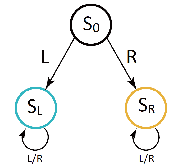
Figure 1: The MDP construction used in the proof of Theorem 14.

Proof.

Define MDP $\mathcal{M}$ with:

• State space ${\mathcal{S}}=\mathinner{\left\{S_{0},S_{L},S_{R}\right\}}$ and action space $\mathcal{A}=\{L,R\}$.

• Initial state distribution $\rho(S_{0})=1$

• Transition dynamics: $P_{1}(S_{L}|S_{0},L)=1$, $P_{1}(S_{R}|S_{0},R)=1$, i.e. playing $L$ at $S_{0}$ transitions to $S_{L}$ deterministically, while playing $R$ at $S_{0}$ transitions to $S_{R}$. Also, $\forall t\in[H-1]$, $\forall a\in\mathcal{A}$, $P_{t}(S_{L}|S_{L},a)=1$, $P_{t}(S_{R}|S_{R},a)=1$, i.e. $S_{L}$ and $S_{R}$ have transition dynamics that are self-absorbing before termination. See Figure 1 for an illustration.

• Cost function $c(S_{0},L)=c(S_{0},R)=c(S_{L},R)=c(S_{R},L)=0$, $c(S_{L},L)=c(S_{R},R)=1$.

Meanwhile, let:

• Benchmark policy class $\mathcal{B}=\{h_{L},h_{R}\}$, where $\forall s$, $h_{L}(s)=L$ and $h_{R}(s)=R$.

• Deterministic expert $\pi^{E}$ such that $\pi^{E}(S_{0})=L$, $\pi^{E}(S_{L})=R$ and $\pi^{E}(S_{R})=L$.

Notice that $\forall s\in{\mathcal{S}}$, $c(s,\pi^{E}(s))=0$, and therefore $V_{\pi^{E}}(s)=0$ for all $s$. Also, by observing $A^{E}(s,a)=Q_{\pi^{E}}(s,a)-V_{\pi^{E}}(s)=c(s,a)$, it can be seen that $A^{E}(S_{0},L)=A^{E}(S_{0},R)=A^{E}(S_{L},R)=A^{E}(S_{R},L)=0$, $A^{E}(S_{L},L)=A^{E}(S_{R},R)=1$.

By the transition dynamics, rolling out $h_{L}$ in $\mathcal{M}$ incurs trajectory $\tau_{h_{L}}=\left(S_{0},L,S_{L},L,\cdots,S_{L},L\right)$ with probability 1, where $A^{E}(S_{0},L)=I(L\neq\pi^{E}(S_{0}))=0$ and $A^{E}(S_{L},L)=I(L\neq\pi^{E}(S_{L}))=1$. Similarly, the trajectory induced by $h_{R}$ is $\tau_{h_{R}}=\left(S_{0},R,S_{R},R,\cdots,S_{R},R\right)$, where $A^{E}(S_{0},R)=0$, $I(R\neq\pi^{E}(S_{0}))=1$ and $A^{E}(S_{R},R)=I(R\neq\pi^{E}(S_{R}))=1$.

For the direct expert annotation feedback $\zeta_{E}(s,a)=\mu\cdot I(a\neq\pi^{E}(s)).$

To begin with, it can be seen from the advantage function values that $(\mathcal{M},\pi^{E})$ is 1-recoverable (i.e. $\forall s\in{\mathcal{S}},a\in\mathcal{A}$, $\left|A^{E}(s,a)\right|\leq 1$). Therefore, the feedback is of the form $\zeta_{E}(s,a)=I(a\neq\pi^{E}(s))$. Recall that $F_{n}(\pi)=\mathbb{E}_{s\sim d_{\pi_{n}}}\mathbb{E}_{a\sim\pi(\cdot|s)}\left[\zeta_{E}(s,a)\right]$, we follow the trajectories of $h_{L},h_{R}$ and obtain:

• when $\pi_{n}=h_{L}$, $F_{n}(h_{L})=\frac{H-1}{H}$, $F_{n}(h_{R})=\frac{1}{H}$.

• when $\pi_{n}=h_{R}$, $F_{n}(h_{R})=1$, $F_{n}(h_{L})=0$.

With this, we conclude that, $\forall\{\pi_{n}\}_{n=1}^{N}\in\{h_{L},h_{R}\}^{N}$, $\sum_{n=1}^{N}F_{n}(\pi_{n})\geq\frac{N(H-1)}{H}$.

On the other hand, $\forall\{\pi_{n}\}_{n=1}^{N}\in\{h_{L},h_{R}\}^{N}$, define $P_{L}\mathrel{\mathop{\mathchar 58\relax}}=\sum_{n=1}^{N}\mathbb{E}_{s\sim d_{\pi_{n}}}I(L=\pi^{E}(s))$, and $P_{R}\mathrel{\mathop{\mathchar 58\relax}}=\sum_{n=1}^{N}\mathbb{E}_{s\sim d_{\pi_{n}}}I(R=\pi^{E}(s))$. For the benchmark term, we have

$$\min_{\pi\in\mathcal{B}}\sum_{n=1}^{N}F_{n}(\pi)=\min\left(\sum_{n=1}^{N}F_{n}(\pi_{L}),\sum_{n=1}^{N}F_{n}(\pi_{R})\right)=\min\left(P_{L},P_{R}\right)\leq\frac{N}{2},$$

where the inequality uses the observation that $P_{L}+P_{R}=N$ and therefore $\min(P_{L},P_{R})\leq\frac{N}{2}$.

Together we obtain $SReg_{N}(\mathcal{B})=\sum_{n=1}^{N}F_{n}(\pi_{n})-\min_{\pi\in\mathcal{B}}\sum_{n=1}^{N}F_{n}(\pi)\geq\frac{N(H-1)}{H}-\frac{N}{2}=\frac{N(H-2)}{2H}$, which is linear in $N$ when $H\geq 3$.

For the feedback of the form $\zeta_{E}(s,a)=A^{E}(s,a).$

By bringing in $\zeta_{E}(s,a)=A^{E}(s,a)$, we obtain $F_{n}(\pi)=\mathbb{E}_{s\sim d_{\pi_{n}}}\mathbb{E}_{a\sim\pi(\cdot|s)}\left[A^{E}(s,a)\right]$, following the trajectories of $h_{L},h_{R}$, it can be seen that:

• when $\pi_{n}=h_{L}$, $F_{n}(h_{L})=\frac{H-1}{H}$,$F_{n}(h_{R})=0$.

• when $\pi_{n}=h_{R}$, $F_{n}(h_{R})=\frac{H-1}{H}$, $F_{n}(h_{L})=0$.

This implies $\forall\{\pi_{n}\}_{n=1}^{N}\in\{h_{L},h_{R}\}^{N}$, $\sum_{n=1}^{N}F_{n}(\pi_{n})=\frac{N(H-1)}{H}.$

On the other hand, $\forall\{\pi_{n}\}_{n=1}^{N}\in\{h_{L},h_{R}\}^{N}$, define $C_{L}\mathrel{\mathop{\mathchar 58\relax}}=\sum_{n=1}^{N}I(\pi_{n}=h_{L})$, and $C_{R}\mathrel{\mathop{\mathchar 58\relax}}=\sum_{n=1}^{N}I(\pi_{n}=h_{R})$, where $C_{L}+C_{R}=N$.

For the benchmark term, we have

$$\min_{\pi\in\mathcal{B}}\sum_{n=1}^{N}F_{n}(\pi)=\min\left(\sum_{n=1}^{N}F_{n}(\pi_{L}),\sum_{n=1}^{N}F_{n}(\pi_{R})\right)=\min\left(C_{L}\frac{H-1}{H},C_{R}\frac{H-1}{H}\right)\leq\frac{N}{2}\cdot\frac{H-1}{H},$$

where the inequality uses the observation that $C_{L}+C_{R}=N$ and therefore $\min(C_{L},C_{R})\leq\frac{N}{2}$.

In conclusion, any online proper learning algorithm satisfies $\mathrm{SReg}_{N}(\mathcal{B})=\sum_{n=1}^{N}F_{n}(\pi_{n})-\min_{\pi\in\mathcal{B}}\sum_{n=1}^{N}F_{n}(\pi)\geq\frac{N(H-1)}{H}-\frac{N(H-1)}{2H}=\frac{N(H-1)}{2H},$ i.e., it suffers regret $\mathrm{SReg}_{N}(\mathcal{B})=\Omega(N)$ which is linear in $N$ when $H\geq 2$. ∎

D.2 Deferred materials from Section 3.2

An alternative mixed policy class and its issues.

Prior work sun2017deeply [Theorem 5.3] propose to use an alternative definition of mixed policy class

$$\tilde{\Pi}_{\mathcal{B}}=\mathinner{\left\{\sigma_{u}\mathrel{\mathop{\mathchar 58\relax}}u\in\Delta(B)\right\}},$$

where policy $\sigma_{u}$ is executed in an an episode of an MDP by: draw $h\sim u$ at the beginning of the episode, and execute policy $h$ throughout the episode. Importantly, $\sigma_{u}$ is not a stationary policy; as a result, $\{a_{t}\}_{t=1}^{H}$ are dependent conditioned on $\{s_{t}\}_{t=1}^{H}$; $\{a_{t}\}_{t=1}^{H}$ are only conditionally independent given $\{s_{t}\}_{t=1}^{H}$ and $h$.

By the definition of $\sigma_{u}$, $J(\sigma_{u})$ is a weighted combination of $J(h)$ over $h\in\mathcal{B}$, which can be written as $J(\sigma_{u})=\sum_{h\in\mathcal{B}}u[h]\cdot J(h)$. sun2017deeply [Theorem 5.3] propose to perform online optimization over the following losses, $\tilde{F}_{n}(\sigma_{u})\mathrel{\mathop{\mathchar 58\relax}}=\mathbb{E}_{s\sim d_{\sigma_{n}}}\left[\sum_{h\in\mathcal{B}}u[h]\cdot A^{E}(s,h(s))\right]$, where $\sigma_{n}$ denotes $\sigma_{u_{n}}$; specifically, they output a sequence of $\mathinner{\left\{u_{n}\right\}}_{n=1}^{N}\subset\Delta(\mathcal{B})$,

$$\sum_{n=1}^{N}\tilde{F}_{n}(\sigma_{n})-\min_{u\in\Delta(\mathcal{B})}\sum_{n=1}^{N}\tilde{F}_{n}(\sigma_{u})\leq\mu\sqrt{N\log(B)}.$$

where $\mathop{\sup}\limits_{s,a}|A^{E}(s,a)|\leq\mu$.

We show by our MDP example in Figure 1 above, in general, $J(\sigma_{n})-J(\pi^{E})\neq H\cdot\tilde{F}_{n}(\sigma_{n}),$ which implies that, an online optimization guarantee for $\{\tilde{F}_{n}(\sigma_{u})\}_{n=1}^{N}$ cannot be converted to a policy suboptimality guarantee. In contrast, in our Logger framework, with the setting of $\zeta_{E}=A^{E}$, we always have that $J(\pi_{n})-J(\pi^{E})=H\cdot F_{n}(\pi_{n})$, which guarantees the conversion.

Consider the MDP in the proof of Theorem 14 and $u_{n}=(0.5,0.5)$. Here, policy $\sigma_{n}$ is executed by picking $h\in\{h_{L},h_{R}\}$ uniformly at random and executing $h$ through the whole episode. Since $J(h_{L})=J(h_{R})=H-1$ and $J(\pi^{E})=0$, we obtain $J(\sigma_{n})-J(\pi^{E})=\sum_{h\in\{h_{L},h_{R}\}}u_{n}[h]\cdot\left(J(h)-J(\pi^{E})\right)=H-1$. On the other side, it can be shown that $d_{\sigma_{n}}$ distributes on $\{S_{0},S_{L},S_{R}\}$ with probability weight $(\frac{1}{H},\frac{H-1}{2H},\frac{H-1}{2H})$, where

$$\sum_{h\in\{h_{L},h_{R}\}}u_{n}[h]\cdot A^{E}(S_{0},h(s))=0,$$

and

$$\sum_{h\in\{h_{L},h_{R}\}}u_{n}[h]\cdot A^{E}(S_{L},h(s))=\sum_{h\in\{h_{L},h_{R}\}}u_{n}[h]\cdot A^{E}(S_{R},h(s))=\frac{1}{2}.$$

Thus it can be verified that $\tilde{F}_{n}(\sigma_{n})=\mathbb{E}_{s\sim d_{\sigma_{n}}}\left[\sum_{h\in\{h_{L},h_{R}\}}u_{n}[h]\cdot A^{E}(s,h(s))\right]=2\cdot\frac{H-1}{2H}\cdot\frac{1}{2}=\frac{H-1}{2H}$. By this we conclude $J(\sigma_{n})-J(\pi^{E})\neq H\cdot\tilde{F}(\sigma_{n})$.

Proof of Proposition 6.

We begin by stating a more precise version of Proposition 6.

Proposition 15 (Restatement of Proposition 6).

For any $\delta\in(0,1]$, if Algorithm 2 uses online linear optimization algorithm $\mathrm{OLOA}$ that outputs $\mathinner{\left\{u_{n}\right\}}_{n=1}^{N}\subset\Delta(\mathcal{B})^{N}$ s.t. with probability at least $1-\delta/3$,

$$\mathrm{LReg}_{N}=\sum_{n=1}^{N}\langle g_{n},u_{n}\rangle-\min_{u\in\Delta(\mathcal{B})}\sum_{n=1}^{N}\langle g_{n},u\rangle\leq\mathrm{Reg}(N).$$

Then, with probability at least $1-\delta$, its output policies $\mathinner{\left\{\pi_{n}\right\}}_{n=1}^{N}$ satisfy

$$\mathrm{SReg}_{N}(\mathcal{B})\leq\mathrm{Reg}(N)+2\mu\sqrt{\frac{2N\ln(\frac{6}{\delta})}{K}}+2\mu\sqrt{2N\frac{\ln(B)+\ln(\frac{6}{\delta})}{K}}=\mathrm{Reg}(N)+O\left(\mu\sqrt{\frac{N\ln(B/\delta)}{K}}\right).$$

Proof.

Recall that in online IL, the loss at round $n$ is $F_{n}(\pi)=\mathbb{E}_{s\sim d_{\pi_{n}}}\mathbb{E}_{a\sim\pi(\cdot\mid s)}\left[\zeta_{E}(s,a)\right]$; For $\pi_{u}\in\Pi_{\mathcal{B}}$,

$$F_{n}(\pi_{u})=\sum_{h\in\mathcal{B}}u[h]\cdot\mathbb{E}_{s\sim d_{\pi_{v}}}\mathbb{E}_{a\sim h(\cdot\mid s)}\left[\zeta_{E}(s,a)\right]=\left\langle\theta(u_{n}),u\right\rangle,$$

where $\theta(v)\mathrel{\mathop{\mathchar 58\relax}}=\left(\mathbb{E}_{s\sim d_{\pi_{n}}}\mathbb{E}_{a\sim h(\cdot\mid s)}\left[\zeta_{E}(s,a)\right]\right)_{h\in\mathcal{B}}$.

In Logger, $g_{n}=\left(\mathbb{E}_{(s,\vec{c})\sim D_{n}}\mathbb{E}_{a\sim h(\cdot\mid s)}\left[\vec{c}(a)\right]\right)_{h\in\mathcal{B}}$ is our unbiased estimator for $\theta(u_{n})$. By defining $f_{n}(\pi)\mathrel{\mathop{\mathchar 58\relax}}=\mathbb{E}_{(s,\vec{c})\sim D_{n}}\mathbb{E}_{a\sim\pi(\cdot|s)}\left[\vec{c}(a)\right]$, it can be seen that $f_{n}(\pi_{u})=\sum_{h\in\mathcal{B}}u[h]\cdot\mathbb{E}_{(s,\vec{c})\sim D_{n}}\mathbb{E}_{a\sim h(\cdot\mid s)}\left[\vec{c}(a)\right]=\langle{g_{n}},{u}\rangle$.

Since the static regret is defined as $\mathrm{SReg}_{N}(\mathcal{B})=\sum_{n=1}^{N}F_{n}(\pi_{n})-\min_{h\in\mathcal{B}}\sum_{n=1}^{N}F_{n}(h)$, where

$$\min_{h\in\mathcal{B}}\sum_{n=1}^{N}F_{n}(h)=\min_{u\in\Delta(\mathcal{B})}\sum_{n=1}^{N}\left\langle\theta(u_{n}),u\right\rangle=\min_{u\in\Delta(\mathcal{B})}\sum_{n=1}^{N}F_{n}(\pi_{u})=\min_{\pi\in\Pi_{\mathcal{B}}}\sum_{n=1}^{N}F_{n}(\pi).$$

We write the static regret as

$$\mathrm{SReg}_{N}(\mathcal{B})=\sum_{n=1}^{N}F_{n}(\pi_{n})-\min_{\pi\in\Pi_{\mathcal{B}}}\sum_{n=1}^{N}F_{n}(\pi)$$

$$=\underbrace{\sum_{n=1}^{N}(F_{n}(\pi_{n})-f_{n}(\pi_{n}))}_{(1)}+\underbrace{\sum_{n=1}^{N}f_{n}(\pi_{n})-\min_{\pi\in\Pi_{\mathcal{B}}}\sum_{n=1}^{N}f_{n}(\pi)}_{(2)}+\underbrace{\min_{\pi\in\Pi_{\mathcal{B}}}\sum_{n=1}^{N}f_{n}(\pi)-\min_{\pi\in\Pi_{\mathcal{B}}}\sum_{n=1}^{N}F_{n}(\pi)}_{(3)}.$$

We will bound each term respectively. First, for (2), we recognize that it equals to $\mathrm{LReg}_{N}=\sum_{n=1}^{N}\langle g_{n},u_{n}\rangle-\min_{u\in\Delta(\mathcal{B})}\sum_{n=1}^{N}\langle g_{n},u\rangle$, which is at most $\mathrm{Reg}(N)$ with probability at least $1-\delta/3$ by the assumptions on $\mathrm{OLOA}$.

We now bound the remaining two terms. Before going into details, we index each cost-sensitive examples as $(s_{n,k},\vec{c}_{n,k})$ for the $k$-th sample that drawn from the $k$-th rollout trajectory at the $n$-th round, where $k\in[K]$, $n\in[N]$ and $\vec{c}_{n,k}=\left(\zeta_{E}(s_{n,k},a)\right)_{a\in\mathcal{A}}$. With this notation, we can write cost-sensitive examples generated at round $n$ as $D_{n}=\left((s_{n,k},\vec{c}_{n,k})\right)_{k=1}^{K}$ and write $f_{n}(\pi)=\mathbb{E}_{(s,\vec{c})\sim D_{n}}\mathbb{E}_{a\sim\pi(\cdot|s)}\left[\vec{c}(a)\right]=\frac{1}{K}\sum_{k=1}^{K}\mathbb{E}_{a\sim\pi(\cdot\mid s_{n,k})}\left[\zeta_{E}(s_{n,k},a)\right]$.

Also, denote $\mathbb{E}_{n,k}\left[Y\right]$ as the conditional expectation of random variable $Y$ on all history before the $k$-th rollout of the $n$-th round. More precisely, denote by $\mathcal{U}_{n,k}=\mathinner{\left\{s_{n^{\prime},k^{\prime}}\mathrel{\mathop{\mathchar 58\relax}}(n^{\prime},k^{\prime})\preceq(n,k)\right\}}$, where $\preceq$ denotes precedence in dictionary order, i.e., $(n_{1},k_{1})\preceq(n_{2},k_{2})$ if and only if $n_{1}<n_{2}$, or $n_{1}=n_{2}$ and $k_{1}\leq k_{2}$; and $\mathbb{E}_{n,k}\left[\cdot\right]\mathrel{\mathop{\mathchar 58\relax}}=\mathbb{E}\left[\cdot\mid\mathcal{U}_{n,k-1}\right]$. As a convention, denote by $\mathcal{U}_{n,0}\mathrel{\mathop{\mathchar 58\relax}}=\mathcal{U}_{n-1,K}$. By the assumption of $\forall s\in{\mathcal{S}},\forall a\in\mathcal{A}$, $A^{E}(s,a)\leq\zeta_{E}(s,a)\leq\mu\cdot I(a\neq\pi^{E}(s))$ and $\left|A^{E}(s,a)\right|\leq\mu$ (recall Section 2), we have that $|\zeta_{E}(s,a)|\leq\mu$ for all $s,a$.

Term (1): $\sum_{n=1}^{N}(F_{n}(\pi_{n})-f_{n}(\pi_{n}))$.

We define $Y_{n,k}\mathrel{\mathop{\mathchar 58\relax}}=F_{n}(\pi_{n})-\mathbb{E}_{a\sim\pi_{n}(\cdot\mid s_{n,k})}\left[\zeta_{E}(s_{n,k},a)\right]$ where $s_{n,k}\sim d_{\pi_{n}}$. It can be seen from the representation of $f_{n}(\pi)=\frac{1}{K}\sum_{k=1}^{K}\mathbb{E}_{a\sim\pi(\cdot\mid s_{n,k})}\left[\zeta_{E}(s_{n,k},a)\right]$ that

$$F_{n}(\pi_{n})-f_{n}(\pi_{n})=\frac{1}{K}\sum_{k=1}^{K}\left(F_{n}(\pi_{n})-\mathbb{E}_{a\sim\pi_{n}(\cdot\mid s_{n,k})}\left[\zeta_{E}(s_{n,k},a)\right]\right)=\frac{1}{K}\sum_{k=1}^{K}Y_{n,k}.$$

Since $\pi_{n}$ only depends on history until $n-1$ round, and $s_{n,k}$ are iid drawn from $d_{\pi_{n}}$, we have

$$\mathbb{E}_{n,k}\left[Y_{n,k}\right]= \mathbb{E}\left[F_{n}(\pi_{n})-\mathbb{E}_{a\sim\pi_{n}(\cdot\mid s_{n,k})}\left[\zeta_{E}(s_{n,k},a)\right]\mid\mathcal{U}_{n,k-1}\right]$$

$$= \mathbb{E}\left[F_{n}(\pi_{n})-\mathbb{E}_{s\sim d_{\pi_{n}}}\mathbb{E}_{a\sim\pi_{n}(\cdot\mid s_{n,k})}\left[\zeta_{E}(s,a)\right]\mid\mathcal{U}_{n-1,K}\right]$$

$$= \mathbb{E}\left[F_{n}(\pi_{n})-F_{n}(\pi_{n})\mid\mathcal{U}_{n-1,K}\right]=0.$$

By applying $\|\zeta_{E}(s_{n,k},\cdot)\|_{\infty}\leq\mu$, we have

$$|Y_{n,k}| =|F_{n}(\pi_{n})-\mathbb{E}_{a\sim\pi_{n}(\cdot\mid s_{n,k})}\left[\zeta_{E}(s_{n,k},a)\right]|$$

$$=|\mathbb{E}_{s\sim d_{\pi_{n}}}\mathbb{E}_{a\sim\pi_{n}(\cdot|s)}\left[\zeta_{E}(s,a)\right]-\left\langle\zeta_{E}(s_{n,k},\cdot),\pi_{n}(\cdot\mid s_{n,k})\right\rangle|$$

$$\leq|\mathbb{E}_{s\sim d_{\pi_{n}}}\left\langle\zeta_{E}(s,\cdot),\pi_{n}(\cdot\mid s)\right\rangle|+\|\zeta_{E}(s_{n,k},\cdot)\|_{\infty}$$

$$\leq 2\|\zeta_{E}(s_{n,k},\cdot)\|_{\infty}\leq 2\mu.$$

This implies the sequence of random variables $\{Y_{1,1},Y_{1,2},\cdots,Y_{1,K},Y_{2,1},\cdots,Y_{N,K}\}$ form a martingale difference sequence. Applying Azuma-Hoeffding’s inequality, we get with probability at least $1-\delta/3$,

$$\left|\sum_{n=1}^{N}(F_{n}(\pi_{n})-f_{n}(\pi_{n}))\right|=\frac{1}{K}\left|\sum_{n=1}^{N}\sum_{k=1}^{K}Y_{n,k}\right|\leq 2\mu\sqrt{\frac{2N{\ln}(\frac{6}{\delta})}{K}}.$$

Term (3): $\min_{\pi\in\Pi_{\mathcal{B}}}\sum_{n=1}^{N}f_{n}(\pi)-\min_{\pi\in\Pi_{\mathcal{B}}}\sum_{n=1}^{N}F_{n}(\pi)$.

Similar to term (1), for any $h\in\mathcal{B}$, we define $\hat{Y}_{n,k}(h)\mathrel{\mathop{\mathchar 58\relax}}=F_{n}(h)-c_{n,k}(h(s_{n,k}),s_{n,k})$ where $s_{n,k}\sim d_{\pi_{n}}$. Also, we have that $f_{n}(\pi)=\frac{1}{K}\sum_{k=1}^{K}\mathbb{E}_{a\sim\pi(\cdot\mid s_{n,k})}\left[\zeta_{E}(s_{n,k},a)\right]$ , which implies $F_{n}(h)-f_{n}(h)=\frac{1}{K}\sum_{k=1}^{K}\hat{Y}_{n,k}(h)$. Following the same analysis shown in term (1), it can be shown that $\mathbb{E}_{n,k}\left[\hat{Y}_{n,k}(h)\right]=0$ and $|\hat{Y}_{n,k}(h)|\leq 2\mu$. By applying Azuma-Hoeffding’s inequality, we get for any given $h\in\mathcal{B}$, with probability at least $1-\frac{\delta}{3B}$ (recall that $B=|\mathcal{B}|$),

$$\left|\sum_{n=1}^{N}(F_{n}(h)-f_{n}(h))\right|=\frac{1}{K}\left|\sum_{n=1}^{N}\sum_{k=1}^{K}\hat{Y}_{n,k}(h)\right|\leq 2\mu\sqrt{2N\frac{\ln(B)+\ln(\frac{6}{\delta})}{K}}.$$

By applying union bound over all $h\in\mathcal{B}$, we get with probability at least $1-\frac{\delta}{3}$, $\sum_{n=1}^{N}(F_{n}(h)-f_{n}(h))\leq 2\mu\sqrt{2N\frac{\ln(B)+\ln(\frac{6}{\delta})}{K}}$, $\forall h\in\mathcal{B}$. Also, by the fact that $f_{n}(\pi)=\langle{g_{n}},{u}\rangle$, it can be shown that

$$\min_{\pi\in\Pi_{\mathcal{B}}}\sum_{n=1}^{N}f_{n}(\pi)=\min_{u\in\Delta(\mathcal{B})}\sum_{n=1}^{N}\langle{g_{n}},{u}\rangle=\min_{h\in\mathcal{B}}\sum_{n=1}^{N}f_{n}(h).$$

Since $\min_{\pi\in\Pi_{\mathcal{B}}}\sum_{n=1}^{N}F_{n}(\pi)=\min_{h\in\mathcal{B}}\sum_{n=1}^{N}F_{n}(h)$, by denoting $h^{*}\in\mathop{\mathrm{argmin}}_{h\in\mathcal{B}}\sum_{n=1}^{N}F_{n}(h)$, we conclude with probability at least $1-\delta/3$ ,

$$\min_{\pi\in\Pi_{\mathcal{B}}}\sum_{n=1}^{N}f_{n}(\pi)-\min_{\pi\in\Pi_{\mathcal{B}}}\sum_{n=1}^{N}F_{n}(\pi)= \min_{h\in\mathcal{B}}\sum_{n=1}^{N}f_{n}(h)-\min_{h\in\mathcal{B}}\sum_{n=1}^{N}F_{n}(h)$$

$$= \min_{h\in\mathcal{B}}\sum_{n=1}^{N}f_{n}(h)-\sum_{n=1}^{N}f_{n}(h^{*})+\sum_{n=1}^{N}(f_{n}(h^{*})-F_{n}(h^{*}))$$

$$\leq 0+2\mu\sqrt{2N\frac{\ln(B)+\ln(\frac{6}{\delta})}{K}}.$$

Finally, by combining our high probability bounds on terms (1),(2), and (3), applying union bound, we conclude that with probability at least $1-\delta$,

$$\begin{aligned} \mathrm{SReg}_{N}(\mathcal{B})\leq&\mathrm{Reg}(N)+2\mu\sqrt{\frac{2N\ln(\frac{6}{\delta})}{K}}+2\mu\sqrt{2N\frac{\ln(B)+\ln(\frac{6}{\delta})}{K}}=\mathrm{Reg}(N)+O\left(\mu\sqrt{\frac{N\ln(B/\delta)}{K}}\right).\end{aligned}\qed$$

Appendix E Deferred materials from Section 4

E.1 Deferred materials from Section 4.1

A more precise version of Lemma 7.

Denote by $\ell=(\ell_{x})_{x\in\mathcal{X}}$ and $q(\ell)=(\sum_{x\in\mathcal{X}}\ell_{x}(h(x)))_{h\in\mathcal{B}}$. Define $\Phi_{\mathcal{N}}\mathrel{\mathop{\mathchar 58\relax}}\mathbb{R}^{B}\to\mathbb{R}$ as:

$$\Phi_{\mathcal{N}}(\Theta)=\mathbb{E}_{\ell\sim\mathcal{N}(0,I_{XA})}\left[\mathop{\max}\limits_{u\in\Delta(\mathcal{B})}\left\langle\Theta+q(\ell),u\right\rangle\right].$$ (4)

Also, define $R_{\mathcal{N}}\mathrel{\mathop{\mathchar 58\relax}}\mathbb{R}^{B}\to\mathbb{R}\cup\mathinner{\left\{+\infty\right\}}$ as $\Phi_{\mathcal{N}}$’s Fenchel conjugate:

$$R_{\mathcal{N}}(u)=\Phi_{\mathcal{N}}^{*}(u)=\sup_{\tilde{\Theta}\in\mathbb{R}^{B}}\left\langle\tilde{\Theta},u\right\rangle-\Phi_{\mathcal{N}}(\tilde{\Theta}).$$ (5)

We will need the following two lemmas that establish properties of $\Phi_{\mathcal{N}}$ and $R$ useful in the proof of Lemma 7; for their proofs, please refer to Section  G.3.

Lemma 16.

$\Phi_{\mathcal{N}}(\Theta)$ is differentiable and $\nabla\Phi_{\mathcal{N}}(\Theta)=\mathbb{E}_{\ell\sim\mathcal{N}(0,I_{XA})}\left[\mathop{\mathop{\mathrm{argmax}}}\limits_{u\in\Delta(\mathcal{B})}\left\langle\Theta+q(\ell),u\right\rangle\right]$.

Lemma 17.

$R_{\mathcal{N}}(u)$ is $\sqrt{\frac{\pi}{8}}{\frac{1}{AX}}$-strongly convex with respect to $\|\cdot\|_{1}$.

Lemma 18.

$\mathop{\mathop{\mathrm{argmin}}}\limits_{u\in\Delta(\mathcal{B})}\left(\langle{\Theta},{u}\rangle+R_{\mathcal{N}}(u)\right)=\nabla\Phi_{\mathcal{N}}(-\Theta)$.

We are now ready to present a more precise version of Lemma 7.

Lemma 19 (A more precise version of Lemma 7).

Suppose Mixed CFTPL receives datasets $\mathinner{\left\{D_{i}\right\}}_{i=1}^{n-1}$, separator set $\mathcal{X}$, learning rate $\eta$, sparsification parameter $T$. Then, $\forall\delta\in(0,1]$, with probability at least $1-\delta$, Mixed CFTPL makes $T$ calls to the cost-sensitive oracle $\mathcal{O}$, and outputs $u_{n}\in\Delta(\mathcal{B})$ s.t.

$$\|\pi_{u_{n}}(\cdot|s)-\pi_{u^{*}_{n}}(\cdot|s)\|_{1}\leq\sqrt{\frac{2A\left(\ln(S)+\ln(\frac{2}{\delta})\right)}{T}},\quad\forall s\in{\mathcal{S}},$$ (6)

with

$$u_{n}^{*}\mathrel{\mathop{\mathchar 58\relax}}=\mathop{\mathrm{argmin}}_{u\in\Delta(\mathcal{B})}\left(\left\langle\eta\sum_{i=1}^{n-1}g_{i},u\right\rangle+R_{\mathcal{N}}(u)\right)=\nabla\Phi_{\mathcal{N}}\left(-\eta\sum_{i=1}^{n-1}g_{i}\right),$$ (7)

for $\Phi_{\mathcal{N}}$ and $R$ defined in Equations (4) and (5).

Proof.

In the proof, we refer to results from online linear optimization, which can be checked in Section G. By Lemma 18 and Lemma 16, for $R_{\mathcal{N}}$ defined in Equation (5) and $\Phi_{\mathcal{N}}$ defined in Equation (4),

$$u_{n}^{*}= \mathop{\mathrm{argmin}}_{u\in\Delta(\mathcal{B})}\left(\left\langle\eta\sum_{i=1}^{n-1}g_{i},u\right\rangle+R_{\mathcal{N}}(u)\right)$$ (8)

$$= \nabla\Phi_{\mathcal{N}}\left(-\eta\sum_{i=1}^{n-1}g_{i}\right)=\mathbb{E}_{\ell\sim\mathcal{N}(0,I_{XA})}\left[\mathop{\mathop{\mathrm{argmax}}}\limits_{u\in\Delta(\mathcal{B})}\left\langle-\eta\sum_{i=1}^{n-1}g_{i}+q(\ell),u\right\rangle\right].$$

We now turn to proving Equation (6). Recall the definition of $u_{n}=\frac{1}{T}\sum_{j=1}^{T}u_{n,j}$ in Algorithm 3, where $u_{n,j}=\operatorname{Onehot}(\mathcal{O}((\cup_{i=1}^{n-1}D_{i})\cup\cup Z_{j}),\mathcal{B})$ and $Z_{j}$ is induced by Gaussian random variables $\ell_{x,j}\sim\mathcal{N}(0,I_{A})$ for each $x\in\mathcal{X}$. Denote by $\ell_{j}=(\ell_{x,j})_{x\in\mathcal{X}}$.

Our proof consists of two steps: first, showing that $\mathbb{E}_{\ell_{j}\sim\mathcal{N}(0,I_{XA})}\left[u_{n,j}\right]=u^{*}_{n}$; second, applying the concentration inequality for Multinoulli random variables on $\|\pi_{u_{n}}(\cdot|s)-\pi_{u_{n}^{*}}(\cdot|s)\|_{1}$ for all $s\in{\mathcal{S}}$.

To begin with, we first prove $\mathbb{E}_{\ell_{j}\sim\mathcal{N}(0,I_{XA})}\left[u_{n,j}\right]=u_{n}^{*}$.

Since each $D_{i}$ contains $K$ cost-sensitive examples, and $\mathcal{X}$ has size $X$, we have $(\cup_{i=1}^{n-1}D_{i})\cup Z_{j}$ contains in total $(n-1)K+X$ examples. Since $g_{i}[h]=\mathbb{E}_{(s,\vec{c})\sim D_{i}}\left[\vec{c}(h(s))\right]$ and $Z_{j}=\mathinner{\left\{(x,\frac{K}{\eta}\ell_{x,j})\mathrel{\mathop{\mathchar 58\relax}}x\in\mathcal{X}\right\}}$, by denoting $q_{j}[h]\mathrel{\mathop{\mathchar 58\relax}}=\sum_{x\in\mathcal{X}}\ell_{x,j}(h(x))$, it can be seen that

$$\mathbb{E}_{(x,\vec{c})\sim(\cup_{i=1}^{n-1}D_{i})\cup Z_{j}}\left[\vec{c}(h(x))\right]$$

$$= \frac{1}{(n-1)K+X}\left(\sum_{i=1}^{n-1}\sum_{(x,\vec{c})\in D_{i}}\vec{c}(h(x))+\sum_{(x,\vec{c})\in Z_{j}}\vec{c}(h(x))\right)$$

$$= \frac{K}{(n-1)K+X}\left(\sum_{i=1}^{n-1}\mathbb{E}_{(x,\vec{c})\sim D_{i}}\left[\vec{c}(h(x))\right]\right)+\frac{1}{(n-1)K+X}\left(\sum_{x\in\mathcal{X}}\frac{K}{\eta}\ell_{x,j}(h(x))\right)$$

$$= \frac{K}{\eta((n-1)K+X)}\left(\eta\sum_{i=1}^{n-1}g_{i}[h]+q_{j}[h]\right).$$

By the definition of oracle $\mathcal{O}$ Definition 3 and $u_{n,j}=\operatorname{Onehot}(\mathcal{O}((\cup_{i=1}^{n-1}D_{i})\cup Z_{j}),\mathcal{B})$,

$$u_{n,j} =\operatorname{Onehot}\left(\mathcal{O}((\cup_{i=1}^{n-1}D_{i})\cup Z_{j}),\mathcal{B}\right)$$

$$=\operatorname{Onehot}\left(\mathop{\mathop{\mathrm{argmin}}}\limits_{h\in\mathcal{B}}\mathbb{E}_{(x,\vec{c})\sim(\cup_{i=1}^{n-1}D_{i})\cup Z_{j}}\left[\vec{c}(h(x))\right],\mathcal{B}\right)$$

$$=\operatorname{Onehot}\left(\mathop{\mathop{\mathrm{argmin}}}\limits_{h\in\mathcal{B}}\frac{K}{\eta((n-1)K+X)}(\eta\sum_{i=1}^{n-1}g_{i}[h]+q_{j}[h]),\mathcal{B}\right)$$

$$=\operatorname{Onehot}\left(\mathop{\mathop{\mathrm{argmin}}}\limits_{h\in\mathcal{B}}(\eta\sum_{i=1}^{n-1}g_{i}[h]+q_{j}[h]),\mathcal{B}\right)$$

$$=\operatorname{Onehot}\left(\mathop{\mathop{\mathrm{argmax}}}\limits_{h\in\mathcal{B}}(-\eta\sum_{i=1}^{n-1}g_{i}[h]-q_{j}[h]),\mathcal{B}\right).$$

By this we obtain

$$\mathbb{E}_{\ell_{j}\sim\mathcal{N}(0,I_{XA})}\left[u_{n,j}\right]=\mathbb{E}_{\ell_{j}\sim\mathcal{N}(0,I_{XA})}\left[\operatorname{Onehot}\left(\mathop{\mathop{\mathrm{argmax}}}\limits_{h\in\mathcal{B}}(-\eta\sum_{i=1}^{n-1}g_{i}[h]-q_{j}[h]),\mathcal{B}\right)\right].$$

On the other hand, we have by Equation (8) that $u_{n}^{*}=\mathbb{E}_{\ell\sim\mathcal{N}(0,I_{XA})}\left[\mathop{\mathop{\mathrm{argmax}}}\limits_{u\in\Delta(\mathcal{B})}\left\langle-\eta\sum_{i=1}^{n-1}g_{i}+q(\ell),u\right\rangle\right]$. By lemma 44 in Section G, under the distribution of $\ell\sim\mathcal{N}(0,I_{XA})$, $\mathop{\mathop{\mathrm{argmin}}}\limits_{u\in\Delta(\mathcal{B})}\left\langle-\eta\sum_{i=1}^{n-1}g_{i}+q(\ell),u\right\rangle$ is unique with probability $1$, which is a one-hot vector. With this observation, we can write

$$u_{n}^{*}= \mathbb{E}_{\ell\sim\mathcal{N}(0,I_{XA})}\left[\mathop{\mathrm{argmax}}\limits_{u\in\Delta(\mathcal{B})}\left\langle-\eta\sum_{i=1}^{n-1}g_{i}+q(\ell),u\right\rangle\right]$$

$$= \mathbb{E}_{\ell\sim\mathcal{N}(0,I_{XA})}\left[\mathop{\mathop{\mathrm{argmax}}}\limits_{u\in\Delta(\mathcal{B})}\left\langle-\eta\sum_{i=1}^{n-1}g_{i}-q(\ell),u\right\rangle\right]$$

$$= \mathbb{E}_{\ell\sim\mathcal{N}(0,I_{XA})}\left[\operatorname{Onehot}(\mathop{\mathop{\mathrm{argmax}}}\limits_{h\in\mathcal{B}}(-\eta\sum_{i=1}^{n-1}g_{i}[h]+q[h]),\mathcal{B})\right],$$

where the first equality uses the following observation: Since $\ell$ is iid from $\mathcal{N}(0,I_{XA})$, $\ell$ and $-\ell$ are equal in distribution. By observing $-q(\ell)=-\left(\sum_{x\in\mathcal{X}}\ell_{x}(h(x)))\right)_{h\in\mathcal{B}}=q(-\ell)$, we have that $q(\ell)$ and $-q(\ell)$ are equal in distribution. This concludes $\mathbb{E}_{\ell_{j}}\left[u_{n,j}\right]=u_{n}^{*}$.

Next, we bound $\|\pi_{u_{n}}(\cdot|s)-\pi_{u^{*}_{n}}(\cdot|s)\|_{1}$.

To this end, we show that for any $s\in{\mathcal{S}}$, $\pi_{u_{n,j}}(\cdot|s)$ is a Multinoulli random variable with expectation $\pi_{u^{*}_{n}}(\cdot|s)$, $\pi_{u}(\cdot|s)=\frac{1}{T}\sum_{j=1}^{T}\pi_{u_{n,j}}(\cdot|s)$, and applying concentration inequality.

Since $u_{n,j}=\operatorname{Onehot}(\mathcal{O}((\cup_{i=1}^{n-1}D_{i})\cup Z_{j}),\mathcal{B})$, which is a one-hot vector, by denoting $h_{n,j}=\mathcal{O}((\cup_{i=1}^{n-1}D_{i})\cup Z_{j})$, it can be seen that $\pi_{u_{n,j}}(\cdot|s)=\sum_{h\in\mathcal{B}}u_{n,j}[h]h(\cdot|s)=h_{n,j}(\cdot|s)$ is also a one-hot vector. Also, $\forall s\in{\mathcal{S}}$,

$$\mathbb{E}_{\ell_{j}\sim\mathcal{N}(0,I_{XA})}\left[\pi_{u_{n,j}}(\cdot|s)\right]=\mathbb{E}_{\ell_{j}\sim\mathcal{N}(0,I_{XA})}\left[\sum_{h\in\mathcal{B}}u_{n,j}[h]h(\cdot|s)\right]=\sum_{h\in B}u^{*}_{n}[h]h(\cdot|s)=\pi_{u^{*}_{n}}(\cdot|s).$$

Thus, $\pi_{u_{n,j}}(\cdot|s)$ can also be seen as Multinoulli random variable on $\Delta(\mathcal{A})$ with expectation $\pi_{u^{*}_{n}}(\cdot|s)$, and $u_{n}$, the empirical average of $u_{n,j}$ satisfies

$$\pi_{u_{n}}(\cdot|s)=\sum_{h\in\mathcal{B}}u_{n}[h]h(\cdot|s)=\sum_{h\in\mathcal{B}}\frac{1}{T}\sum_{i=1}^{T}u_{n,j}[h]h(\cdot|s)=\frac{1}{T}\sum_{i=1}^{T}\pi_{u_{n,j}}(\cdot|s).$$

Thus, we apply concentration inequality for Multinoulli random variables qian2020concentration (originally weissman2003inequalities [Theorem 2.1]) on $\pi_{u_{n}}(\cdot|s)$ and obtain given any $s\in{\mathcal{S}}$, with probability at least $1-\delta/S$,

$$\|\pi_{u_{n}}(\cdot|s)-\pi_{u^{*}_{n}}(\cdot|s)\|_{1}<\sqrt{\frac{2A\left(\ln(S)+\ln(\frac{2}{\delta})\right)}{T}}.$$

By applying union bound over all states in ${\mathcal{S}}$, we conclude that, with probability at least $1-\delta$,

$$\|\pi_{u_{n}}(\cdot|s)-\pi_{u^{*}_{n}}(\cdot|s)\|_{1}\leq\sqrt{\frac{2A\left(\ln(S)+\ln(\frac{2}{\delta})\right)}{T}},\forall s\in{\mathcal{S}}.\qed$$

Lemma 20 (Restatement of Lemma 8).

For any $\delta\in(0,1]$, MFTPL, if being called for $N$ rounds, with input learning rate $\eta=\frac{1}{\mu\sqrt{NA}}(\frac{\ln(B)}{X})^{\frac{1}{4}}$ and sparsification parameter $T=\frac{N\ln(2NS/\delta)}{\sqrt{X^{3}\ln(B)}}$, outputs a sequence of $\mathinner{\left\{u_{n}\right\}}_{n=1}^{N}$, such that with probability $1-\delta$:

$$\mathrm{LReg}_{N}=\sum_{n=1}^{N}\langle{g_{n}},{u_{n}}\rangle-\min_{u\in\Delta(\mathcal{B})}\sum_{n=1}^{N}\langle{g_{n}},{u}\rangle\leq O\left(\mu\sqrt{NA}(X^{3}\ln(B))^{\frac{1}{4}}\right).$$

Proof.

Denote $u_{n}^{*}=\nabla\Phi_{\mathcal{N}}(-\eta\sum_{i=1}^{n-1}g_{i})$ the same as Equation (7), where $g_{n}=\left(\mathbb{E}_{(s,\vec{c})\sim D_{n}}\left[\vec{c}(h(s))\right]\right)_{h\in\mathcal{B}}$, we rewrite the regret as

$$\mathrm{LReg}_{N}=\underbrace{\sum_{n=1}^{N}\langle{g_{n}},{u_{n}}\rangle-\sum_{n=1}^{N}\langle{g_{n}},{u^{*}_{n}}\rangle}_{(1)}+\underbrace{\sum_{n=1}^{N}\langle{g_{n}},{u^{*}_{n}}\rangle-\min_{u\in\Delta(\mathcal{B})}\sum_{n=1}^{N}\langle{g_{n}},{u}\rangle}_{(2)}.\\$$

Term (1): $\sum_{n=1}^{N}\langle{g_{n}},{u_{n}}\rangle-\sum_{n=1}^{N}\langle{g_{n}},{u^{*}_{n}}\rangle$.

For the first term, instead of bounding it naively by $\|u_{n}-u_{n}^{*}\|_{1}$, we expand its definition and use Lemma 19 to give a tighter bound. Denote $\pi_{n}^{*}=\pi_{u_{n}^{*}}$, by Lemma 19, we guarantee that for any round $n$, with probability at least $1-\delta/N$,

$$\langle{g_{n}},{u_{n}-u^{*}_{n}}\rangle= \mathbb{E}_{(x,\vec{c})\sim D_{n}}\mathbb{E}_{a\sim\pi_{n}(\cdot|s)}\left[\vec{c}(a)\right]-\mathbb{E}_{(x,\vec{c})\sim D_{n}}\mathbb{E}_{a\sim\pi_{n}^{*}(\cdot|s)}\left[\vec{c}(a)\right]$$

$$= \mathbb{E}_{(x,\vec{c})\sim D_{n}}\left[\left\langle\vec{c},\pi_{n}(\cdot|x)-\pi_{n}^{*}(\cdot|x)\right\rangle\right]$$

$$\leq \mathbb{E}_{(x,\vec{c})\sim D_{n}}\left[\|\pi_{n}(\cdot|x)-\pi_{n}^{*}(\cdot|x)\|_{1}\|\vec{c}\|_{\infty}\right]$$

$$\leq \mu\sqrt{2A\frac{\ln(NS)+\ln(\frac{2}{\delta})}{T}},$$

where the last line is form applying $\|\vec{c}\|_{\infty}=\|\zeta_{E}(x,\cdot)\|_{\infty}\leq\mu$, and with probability at least $1-\delta/N$, for all $s\in{\mathcal{S}}$, $\|\pi_{u_{n}}(\cdot|s)-\pi_{u^{*}_{n}}(\cdot|s)\|_{1}\leq\sqrt{2A\frac{\ln(NS)+\ln(\frac{2}{\delta})}{T}}$. Then, by applying union bound for $N$ rounds, and sum over $n\in[N]$ we obtain that with probability at least $1-\delta$,

$$\sum_{n=1}^{N}\langle{g_{n}},{u_{n}}\rangle-\sum_{n=1}^{N}\langle{g_{n}},{u^{*}_{n}}\rangle\leq\mu N\sqrt{\frac{2A\left(\ln(NS)+\ln(\frac{2}{\delta})\right)}{T}}.$$

Term (2): $\sum_{n=1}^{N}\langle{g_{n}},{u^{*}_{n}}\rangle-\min_{u\in\Delta(\mathcal{B})}\sum_{n=1}^{N}\langle{g_{n}},{u}\rangle$.

By the definition of $u^{*}_{n}=\nabla\Phi_{\mathcal{N}}(-\eta\sum_{i=1}^{n-1}g_{i})$, $u_{n}^{*}$ follows exactly the same update rule of Algorithm 6 with $\Phi_{\mathcal{N}}$ defined in Equation (4), on online loss $g_{n}$ and optimistic estimation $\hat{g}_{n}$ set to be $0$ for all $n$. By Theorem 53, the regret of $\mathinner{\left\{u_{n}^{*}\right\}}_{n=1}^{N}$ is bounded by

$$\sum_{n=1}^{N}\left\langle g_{n},u^{*}_{n}\right\rangle-\min_{u\in\Delta(\mathcal{B})}\sum_{n=1}^{N}\left\langle g_{n},u\right\rangle\leq \frac{1}{\eta}\sqrt{2X\ln(B)}+\sum_{n=1}^{N}XA\eta\|g_{n}\|_{\infty}^{2}$$

$$\leq \frac{1}{\eta}\sqrt{2X\ln(B)}+\eta\mu^{2}NXA,$$

where we use the fact that $g_{n}=\left(\mathbb{E}_{(s,\vec{c})\sim D_{n}}\left[\vec{c}(h(s))\right]\right)_{h\in\mathcal{B}}$ has $\|g_{n}\|_{\infty}$ at most $\mu$ as $\|\zeta_{E}(s,\cdot)\|_{\infty}\leq\mu$ for all $s$.

Finally, by combining the bounds on the first and second terms together, we obtain $\forall\delta\in(0,1]$, with probability at least $1-\delta$,

$$\sum_{n=1}^{N}\langle{g_{n}},{u_{n}}\rangle-\min_{u\in\Delta(\mathcal{B})}\sum_{n=1}^{N}\langle{g_{n}},{u}\rangle\leq\frac{1}{\eta}\sqrt{2X\ln(B)}+\eta\mu^{2}NXA+\mu N\sqrt{2A\frac{\ln(NS)+\ln(\frac{2}{\delta})}{T}}.$$

By setting $\eta=\frac{1}{\mu\sqrt{NA}}\left(\frac{\ln(B)}{X}\right)^{\frac{1}{4}}$ and $T=\frac{N\ln(2NS/\delta)}{\sqrt{X^{3}\ln(B)}}$, we conclude with probability at least $1-\delta$,

$$\begin{aligned} \mathrm{LReg}_{N}\leq\left(1+\frac{\sqrt{2}}{2}+1\right)\mu\sqrt{2NA}\left(X^{3}\ln(B)\right)^{\frac{1}{4}}=O\left(\mu\sqrt{NA}\left(X^{3}\ln(B)\right)^{\frac{1}{4}}\right).\end{aligned}\qed$$

Theorem 21 (Restatement of Theorem 9).

For any $\delta\in(0,1]$, Logger-M, with MFTPL setting its parameters as in Lemma 8 and $K=1$, satisfies that: (1) with probability at least $1-\delta$, its output $\mathinner{\left\{\pi_{n}\right\}}_{n=1}^{N}$ satisfies: $\mathrm{SReg}(N)\leq O\left(\mu\sqrt{NA\ln(1/\delta)}(X^{3}\ln(B))^{\frac{1}{4}}\right)$; (2) it queries $N$ annotations from expert $\pi^{E}$; (3) it calls the CSC oracle $\mathcal{O}$ for $\frac{N^{2}\ln(6NS/\delta)}{\sqrt{X^{3}\ln(B)}}$ times.

Specifically, Logger-M achieves $\frac{H}{N}\mathrm{SReg}_{N}(\mathcal{B})\leq\epsilon$ with probability at least $1-\delta$ in $N=O\left(\frac{\mu^{2}H^{2}A\ln(1/\delta)\sqrt{X^{3}\ln(B)}}{\epsilon^{2}}\right)$ interaction rounds, with $O\left(\frac{\mu^{2}H^{2}A\ln(1/\delta)\sqrt{X^{3}\ln(B)}}{\epsilon^{2}}\right)$ expert annotations and $\tilde{O}\left(\frac{\mu^{4}H^{4}A^{2}\left(\ln(1/\delta)\right)^{2}\ln(S/\delta)\sqrt{X^{3}\ln(B)}}{\epsilon^{4}}\right)$ oracle calls.

Proof.

Following the results in Lemma 8, MFTPL, if being called for $N$ rounds with the prescribed input learning rate $\eta$ and sparsification parameter $T=\frac{N\ln(6NS/\delta)}{\sqrt{X^{3}\ln(B)}}$, generates a sequence of $\mathinner{\left\{u_{n}\right\}}_{n=1}^{N}$, such that with probability at least $1-\frac{\delta}{3}$,

$$\mathrm{LReg}_{N}\leq O\left(\mu\sqrt{NA}(X^{3}\ln(B))^{\frac{1}{4}}\right).$$

By Proposition 6, Logger-M output policies $\mathinner{\left\{\pi_{n}\right\}}_{n=1}^{N}$ such that with probability at least $1-\delta$,

$$\mathrm{SReg}_{N}(\mathcal{B})\leq O\left(\mu\sqrt{NA}(X^{3}\ln(B))^{\frac{1}{4}}\right)+O\left(\mu\sqrt{\frac{N\ln(B/\delta)}{K}}\right).$$

By setting $K=1$, we obtain

$$\mathrm{SReg}_{N}(\mathcal{B})\leq O\left(\mu\sqrt{NA}(X^{3}\ln(B))^{\frac{1}{4}}\right)+O\left(\mu\sqrt{N(\ln(B/\delta))}\right)=O\left(\mu\sqrt{NA\ln(1/\delta)}(X^{3}\ln(B))^{\frac{1}{4}}\right),$$

where $O\left(\mu\sqrt{N\ln(B/\delta)}\right)$ is of lower order, by $X\geq\log_{A}(B)$ proven in Lemma 56.

Since at each round, Algorithm 2 queries $K=1$ annotation from the expert and calls MFTPL once, where MFTPL calls oracle $\mathcal{O}$ $T=\frac{N\ln(6NS/\delta)}{\sqrt{X^{3}\ln(B)}}$ times, then for a total of $N$ rounds, it calls $N$ annotations and calls oracle $\mathcal{O}$ for $\frac{N^{2}\ln(6NS/\delta)}{\sqrt{X^{3}\ln(B)}}$ times.

For the second part of the theorem, to guarantee $\frac{H}{N}\mathrm{SReg}_{N}(\mathcal{B})\leq\epsilon$, it suffices to let $N=O\left(\frac{\mu^{2}H^{2}A\ln(1/\delta)\sqrt{X^{3}\ln(B)}}{\epsilon^{2}}\right)$. The number of annotations and oracle calls follow from plugging this value of $N$ into their settings in the first part of the theorem. ∎

E.2 Deferred materials from Section 4.2

E.2.1 The MFTPL-EG algorithm and its guarantees

We present MFTPL-EG (Algorithm 4), an alternative to MFTPL (Algorithm 3) for online linear optimization in COIL. Recall that in the Logger framework, for every $n$, the linear loss $g_{n}$ at round $n$ is induced by $D_{n}$, in that $g_{n}[h]=\mathbb{E}_{(s,c)\sim D_{n}}\left[\vec{c}(h(s))\right]$ for all $h\in\mathcal{B}$.

Specifically, at round $n$, MFTPL-EG first computes $\hat{u}_{n}$, the output of MFTPL on $\{g_{i}\}_{i=1}^{n-1}$ (line 1); different from MFTPL, instead of using this as $u_{n}$, it rather uses this as a estimator for $u_{n}$, which is still to be determined at this point. $\hat{u}_{n}$ induces policy $\hat{\pi}_{n}=\pi_{\hat{u}_{n}}$. After rolling out $\hat{\pi}_{n}$ in $\mathcal{M}$ and requesting expert annotations (line 2), we obtain a dataset $\hat{D}_{n}$, whose induced linear loss (denoted by $\hat{g}_{n}$), is an unbiased estimate of $\theta(\hat{u}_{n})$, which by the distributional continuity property (Lemma 10), turns out to be a good estimator of $\theta(u_{n})$. Finally, MFTPL-EG calls MFTPL on the linear losses $\mathinner{\left\{g_{i}\right\}}_{i=1}^{n-1}\cup\mathinner{\left\{\hat{g}_{n}\right\}}$ (line 3).

Algorithm 4 Mixed CFTPL with Extra Gradient (abbrev. MFTPL-EG)

0:  MDP $\mathcal{M}$, expert feedback $\zeta_{E}$, Linear losses $\{g_{i}\}_{i=1}^{n-1}$ represented by datasets $\mathinner{\left\{D_{i}\right\}}_{i=1}^{n-1}$ each of size $K$ (s.t. $g_{i}[h]=\mathbb{E}_{(s,\vec{c})\sim D_{i}}\left[\vec{c}(h(s))\right]$ for all $h\in\mathcal{B}$), separator set $\mathcal{X}$, learning rate $\eta$, sparsification parameter $T$.

1:  $\hat{u}_{n}\leftarrow\textsc{MFTPL}\left(\mathinner{\left\{D_{i}\right\}}_{i=1}^{n-1},\mathcal{X},\eta,T\right)$, and let $\hat{\pi}_{n}\leftarrow\pi_{\hat{u}_{n}}$.

2:  Draw $K$ examples $\hat{D}_{n}=\mathinner{\left\{(s,\vec{c})\right\}}$ iid from $D_{\hat{\pi}_{n},E}$, via interaction with $\mathcal{M}$ and expert $\zeta_{E}$.

3:  return  $u_{n}\leftarrow\textsc{MFTPL}\left(\mathinner{\left\{D_{i}\right\}}_{i=1}^{n-1}\cup\hat{D}_{n},\mathcal{X},\eta,T\right)$.

To analyze MFTPL-EG, We first restate and prove a distributional continuity property in COIL problems.

Lemma 22 (Restatement of Lemma 10).

For any $u,v\in\Delta(\mathcal{B})$,

$$\|\theta(u)-\theta(v)\|_{\infty}\;\begin{subarray}{c}(*1)\\ \leq\end{subarray}\;\mu H\max_{s\in{\mathcal{S}}}\|\pi_{u}(\cdot|s)-\pi_{v}(\cdot|s)\|_{1}\;\begin{subarray}{c}(*2)\\ \leq\end{subarray}\;\mu H\|u-v\|_{1}.$$

Proof.

We show $(*1)$ and $(*2)$ respectively.

For $(*1)$, recall the definition of trajectory as $\tau=\{s_{1},a_{1},\cdots,s_{H},a_{H}\}$, we abuse $d_{\pi}(\cdot)$ to denote the distribution of trajectory induced by policy $\pi$. By denoting $\theta_{u}[h]=\mathbb{E}_{s\sim d_{\pi_{u}}}\left[\zeta_{E}(s,h(s))\right]$ and $\theta_{v}[h]=\mathbb{E}_{s\sim d_{\pi_{v}}}\left[\zeta_{E}(s,h(s))\right]$, we have for any $h\in\mathcal{B}$:

$$\left|\theta_{u}[h]-\theta_{v}[h]\right|= \left|\mathbb{E}_{s\sim d_{\pi_{u}}}\left[\zeta_{E}(s,h(s))\right]-\mathbb{E}_{s\sim d_{\pi_{v}}}\left[\zeta_{E}(s,h(s))\right]\right|$$

$$= \left|\mathbb{E}_{\tau\sim d_{\pi_{u}}(\cdot)}\left[\frac{1}{H}\sum_{s\in\tau}\zeta_{E}(s,h(s))\right]-\mathbb{E}_{\tau\sim d_{\pi_{v}}(\cdot)}\left[\frac{1}{H}\sum_{s\in\tau}\zeta_{E}(s,h(s))\right]\right|$$

$$= \left|\sum_{\tau\in({\mathcal{S}}\times\mathcal{A})^{H}}\left((d_{\pi_{u}}(\tau)-d_{\pi_{v}}(\tau))\cdot\frac{1}{H}\sum_{s\in\tau}\zeta_{E}(s,h(s))\right)\right|$$

$$\leq \left|\sum_{\tau\in({\mathcal{S}}\times\mathcal{A})^{H}}\mu(d_{\pi_{u}}(\tau)-d_{\pi_{v}}(\tau))\right|$$

$$= \mu\cdot\|d_{\pi_{u}}(\cdot)-d_{\pi_{v}}(\cdot)\|_{1}=2\mu\cdot D_{\mathrm{TV}}\left(d_{\pi_{u}}(\cdot),d_{\pi_{v}}(\cdot)\right).$$

where the last inequality is by $\forall s\in{\mathcal{S}}$, $\forall a\in\mathcal{A}$, $\left|\zeta_{E}(s,a)\right|\leq\mu$. Here, $D_{\mathrm{TV}}(u,v)\mathrel{\mathop{\mathchar 58\relax}}=\frac{1}{2}\|u-v\|_{1}$ denotes the Total Variance (TV) distance between two distributions.

Now, by ke2020imitation [Theorem 4]:

$$D_{\mathrm{TV}}\left(d_{\pi_{u}}(\cdot),d_{\pi_{v}}(\cdot)\right)\leq H\cdot\mathbb{E}_{s\sim d_{\pi_{u}}}\left[D_{\mathrm{TV}}\left(\pi_{u}(\cdot\mid s),\pi_{v}(\cdot\mid s)\right)\right],$$ (9)

we utilize Equation (9) and conclude that for any $h\in\mathcal{B}$,

$$\left|\theta_{u}[h]-\theta_{v}[h]\right|\leq 2\mu\cdot D_{\mathrm{TV}}\left(d_{\pi_{u}}(\cdot),d_{\pi_{v}}(\cdot)\right)$$

$$\leq 2\mu H\cdot\mathbb{E}_{s\sim d_{\pi_{u}}}\left[D_{\mathrm{TV}}\left(\pi_{u}(\cdot\mid s),\pi_{v}(\cdot\mid s)\right)\right]$$

$$\leq 2\mu H\max_{s\in{\mathcal{S}}}D_{\mathrm{TV}}\left(\pi_{u}(\cdot\mid s),\pi_{v}(\cdot\mid s)\right)$$

$$= \mu H\max_{s\in{\mathcal{S}}}\|\pi_{u}(\cdot|s)-\pi_{v}(\cdot|s)\|_{1}.$$

For $(*2)$, by the definition of $\pi_{u_{n}}(\cdot|s)=\sum_{h\in\mathcal{B}}u[h]h(\cdot|s)$, we have that $\forall s\in{\mathcal{S}}$,

$$\|\pi_{u}(\cdot|s)-\pi_{v}(\cdot|s)\|_{1} =\|\sum_{h\in\mathcal{B}}u[h]h(\cdot|s)-\sum_{h\in\mathcal{B}}v[h]h(\cdot|s)\|_{1}$$

$$=\sum_{a\in\mathcal{A}}\left|\sum_{h\in\mathcal{B}}(u[h]-v[h])I(h(s)=a)\right|$$

$$\leq\sum_{a\in\mathcal{A}}\sum_{h\in\mathcal{B}}\left|u[h]-v[h]\right|I(h(s)=a)$$

$$=\sum_{h\in\mathcal{B}}\sum_{a\in\mathcal{A}}\left|u[h]-v[h]\right|I(h(s)=a)$$

$$=\sum_{h\in\mathcal{B}}\left|u[h]-v[h]\right|=\|u-v\|_{1}.$$

This lets us conclude

$$\|\theta(u)-\theta(v)\|_{\infty}=\max_{h\in\mathcal{B}}|\theta_{u}[h]-\theta_{v}[h]|\leq\mu H\max_{s\in{\mathcal{S}}}\|\pi_{u}(\cdot|s)-\pi_{v}(\cdot|s)\|_{1}\leq\mu H\|u-v\|_{1}.\qed$$

Lemma 23.

Let $N\geq\mu HA\sqrt{X^{3}\ln(B)}$. For any $\delta\in(0,1]$, if MFTPL-EG is called for $N$ rounds, with input learning rate $\eta=\frac{1}{5\mu HAX}$, sparsification parameter $T=\frac{N^{2}\ln(8NS/\delta)}{\mu HAX^{3}\ln(B)}$ and sample budget $K=\frac{N\ln(8NB/\delta)}{H^{2}A\sqrt{X^{3}\ln(B)}}$ , outputs a sequence $\mathinner{\left\{u_{n}\right\}}_{n=1}^{N}$, such that with probability at least $1-\delta$:

$$\mathrm{LReg}_{N}\leq O\left(\mu HA\sqrt{X^{3}\ln(B)}\right).$$

Proof.

We will follow a proof outline similar to that of Lemma 20; intuitively, we can view MFTPL-EG as approximating the execution of Algorithm 6.

At the $n$-th round in the execution of MFTPL-EG, the algorithm calls MFTPL with dataset $\mathinner{\left\{D_{i}\right\}}_{i=1}^{n-1}$ to get $\hat{u}_{n}$ and gather extra data set $\hat{D}_{n}$ by rolling out $\hat{\pi}_{n}=\pi_{\hat{u}_{n}}$ in $\mathcal{M}$. Then it outputs $u_{n}$ by running MFTPL on $\mathinner{\left\{D_{i}\right\}}_{i=1}^{n-1}\cup\hat{D}_{n}$.

In parallel to the definition that $g_{n}=\left(\mathbb{E}_{(s,\vec{c})\sim D_{n}}\left[\vec{c}(h(s))\right]\right)_{h\in\mathcal{B}}$, we denote the loss vector induced by $\hat{D}_{n}$ as $\hat{g}_{n}=\left(\mathbb{E}_{(s,\vec{c})\sim\hat{D}_{n}}\left[\vec{c}(h(s))\right]\right)_{h\in\mathcal{B}}$. Following a similar definition as Equation (7), we denote $\hat{u}^{*}_{n}\mathrel{\mathop{\mathchar 58\relax}}=\nabla\Phi_{\mathcal{N}}(-\eta\sum_{i=1}^{n-1}g_{i})$ and $u^{*}_{n}\mathrel{\mathop{\mathchar 58\relax}}=\nabla\Phi_{\mathcal{N}}(-\eta(\sum_{i=1}^{n-1}g_{i}+\hat{g}_{n}))$. We first rewrite the online linear optimization regret in the same way as the proof of Lemma 20 using $u_{n}^{*}$,

$$\mathrm{LReg}_{N}=\underbrace{\sum_{n=1}^{N}\langle{g_{n}},{u_{n}}\rangle-\sum_{n=1}^{N}\langle{g_{n}},{u^{*}_{n}}\rangle}_{(1)}+\underbrace{\sum_{n=1}^{N}\langle{g_{n}},{u^{*}_{n}}\rangle-\min_{u\in\Delta(\mathcal{B})}\sum_{n=1}^{N}\langle{g_{n}},{u}\rangle}_{(2)},$$

and bound terms (1) and (2) respectively.

Term (1): $\sum_{n=1}^{N}\langle{g_{n}},{u_{n}}\rangle-\sum_{n=1}^{N}\langle{g_{n}},{u^{*}_{n}}\rangle$.

Since $u_{n}$ is the output from MFTPL with input dataset $\mathinner{\left\{D_{i}\right\}}_{i=1}^{n-1}\cup\hat{D}_{n}$, separator set $\mathcal{X}$, and learning rate $\eta$ , while $u^{*}_{n}\mathrel{\mathop{\mathchar 58\relax}}=\nabla\Phi_{\mathcal{N}}(-\eta(\sum_{i=1}^{n-1}g_{i}+\hat{g}_{n}))$ is induced by $\mathinner{\left\{D_{i}\right\}}_{i=1}^{n-1}$ and $\hat{g}_{n}$ is induced by $\hat{D}_{n}$. We apply Lemma 19 and guarantee for any given round $n$, with probability at least $1-\frac{\delta}{4N}$, for all $s\in{\mathcal{S}}$, $\|\pi_{u_{n}}(\cdot|s)-\pi_{u^{*}_{n}}(\cdot|s)\|_{1}\leq\sqrt{2A\frac{\ln(NS)+\ln(\frac{8}{\delta})}{T}}$. By applying union bound over $N$ rounds, we obtain that event $E_{1}$ happens with probability at least $1-\frac{\delta}{4}$, where $E_{1}$ is defined as

$$E_{1}\mathrel{\mathop{\mathchar 58\relax}}\|\pi_{u_{n}}(\cdot|s)-\pi_{u^{*}_{n}}(\cdot|s)\|_{1}\leq\sqrt{2A\frac{\ln(NS)+\ln(\frac{8}{\delta})}{T}},\forall n\in[N],\forall s\in{\mathcal{S}}.$$ (10)

Thus, when $E_{1}$ happens, $\forall n\in[N]$,

$$\langle{g_{n}},{u_{n}-u^{*}_{n}}\rangle= \mathbb{E}_{(x,\vec{c})\sim D_{n}}\mathbb{E}_{a\sim\pi_{n}(\cdot|s)}\left[\vec{c}(a)\right]-\mathbb{E}_{(x,\vec{c})\sim D_{n}}\mathbb{E}_{a\sim\pi_{n}^{*}(\cdot|s)}\left[\vec{c}(a)\right]$$

$$= \mathbb{E}_{(x,\vec{c})\sim D_{n}}\left[\left\langle\vec{c},\pi_{n}(\cdot|x)-\pi_{n}^{*}(\cdot|x)\right\rangle\right]$$

$$\leq \mathbb{E}_{(x,\vec{c})\sim D_{n}}\left[\|\pi_{n}(\cdot|x)-\pi_{n}^{*}(\cdot|x)\|_{1}\|\vec{c}\|_{\infty}\right]$$

$$\leq \mu\sqrt{2A\frac{\ln(NS)+\ln(\frac{8}{\delta})}{T}},$$

which implies,

$$\sum_{n=1}^{N}\langle{g_{n}},{u_{n}}\rangle-\sum_{n=1}^{N}\langle{g_{n}},{u^{*}_{n}}\rangle\leq\mu N\sqrt{2A\frac{\ln(NS)+\ln(\frac{8}{\delta})}{T}}.$$

Term (2): $\sum_{n=1}^{N}\langle{g_{n}},{u^{*}_{n}}\rangle-\min_{u\in\Delta(\mathcal{B})}\sum_{n=1}^{N}\langle{g_{n}},{u}\rangle$.

By the definition of $u^{*}_{n}\mathrel{\mathop{\mathchar 58\relax}}=\nabla\Phi_{\mathcal{N}}(-\eta(\sum_{i=1}^{n-1}g_{i}+\hat{g}_{n}))$, $u^{*}_{n}$ follows the update rule of Algorithm 6 with $\Phi_{\mathcal{N}}$ defined in Equation (4), online loss $g_{n}$ and optimistic estimation $\hat{g}_{n}$. By Theorem 53, the regret is bounded by

$$\sum_{n=1}^{N}\left\langle g_{n},u^{*}_{n}\right\rangle-\min_{u\in\Delta(\mathcal{B})}\sum_{n=1}^{N}\left\langle g_{n},u\right\rangle$$

$$\leq \frac{1}{\eta}\sqrt{2X\ln(B)}+\sum_{n=1}^{N}\left(\eta AX\|g_{n}-\hat{g}_{n}\|_{\infty}^{2}-\frac{1}{4\eta AX}\|u_{n}^{*}-\hat{u}_{n}^{*}\|_{1}^{2}\right),$$

where we applied the fact that $\nabla\Phi_{\mathcal{N}}(-\eta(\sum_{i=1}^{n-1}g_{i}+\hat{g}_{n}))-\nabla\Phi_{\mathcal{N}}(-\eta(\sum_{i=1}^{n-1}g_{i}))=u_{n}^{*}-\hat{u}_{n}^{*}$.

We now turn to bound $\|g_{n}-\hat{g}_{n}\|_{\infty}^{2}$. Intuitively, $g_{n}$ and $\hat{g}_{n}$ are approximators of $\theta(u_{n}^{*})$ and $\theta(\hat{u}_{n}^{*})$, while by the inequality $(*2)$ of Lemma 22, $\|\theta(u_{n}^{*})-\theta(\hat{u}_{n}^{*})\|_{\infty}\leq\mu H\|u_{n}^{*}-\hat{u}_{n}^{*}\|_{1}$. By cheng2019accelerating [Lemma H.3], we bound $\|g_{n}-\hat{g}_{n}\|_{\infty}^{2}$ by

$$\|g_{n}-\hat{g}_{n}\|_{\infty}^{2}\leq 5\cdot(\underbrace{\|g_{n}-\theta(u_{n})\|_{\infty}^{2}}_{(a)}+\underbrace{\|\theta(u_{n})-\theta(u_{n}^{*})\|_{\infty}^{2}}_{(b)}+\underbrace{\|\theta(u_{n}^{*})-\theta(\hat{u}_{n}^{*})\|_{\infty}^{2}}_{(c)}$$

$$+\underbrace{\|\theta(\hat{u}_{n}^{*})-\theta(\hat{u}_{n})\|_{\infty}^{2}}_{(\tilde{b})}+\underbrace{\|\theta(\hat{u}_{n})-\hat{g}_{n}\|_{\infty}^{2}}_{(\tilde{a})}).$$

We group the terms in three groups: $(a)(\tilde{a})$, $(b)(\tilde{b})$, and $(c)$, and apply different techniques to bound them. For the easiest $(c)$ term, we apply Lemma 22 and bound it by $\|\theta(u_{n}^{*})-\theta(\hat{u}_{n}^{*})\|_{\infty}^{2}\leq\mu^{2}H^{2}\|u_{n}^{*}-\hat{u}_{n}^{*}\|^{2}_{1}$.

For $(b)$ and $(\tilde{b})$, we apply inequality $(*1)$ in Lemma 22 and get

$$\|\theta(u_{n})-\theta(u_{n}^{*})\|_{\infty}^{2}\leq \mu^{2}H^{2}\max_{s\in{\mathcal{S}}}\|\pi_{u_{n}}(\cdot|s)-\pi_{u_{n}^{*}}(\cdot|s)\|_{1}^{2},$$

$$\|\theta(\hat{u}_{n}^{*})-\theta(\hat{u}_{n})\|_{\infty}^{2}\leq \mu^{2}H^{2}\max_{s\in{\mathcal{S}}}\|\pi_{\hat{u}_{n}}(\cdot|s)-\pi_{\hat{u}_{n}^{*}}(\cdot|s)\|_{1}^{2}.$$

For term $(b)$, on event $E_{1}$, which happens with probability $1-\frac{\delta}{4}$, we have that $\max_{s\in{\mathcal{S}}}\|\pi_{u_{n}}(\cdot|s)-\pi_{u_{n}^{*}}(\cdot|s)\|_{1}^{2}\leq 2A\frac{\ln(NS)+\ln(\frac{8}{\delta})}{T}$ for all $n\in[N]$. For term $(\tilde{b})$, the same analysis goes through for $\hat{u}_{n}$ the output from MFTPL with input dataset $\mathinner{\left\{D_{i}\right\}}_{i=1}^{n-1}$, and $\hat{u}^{*}_{n}\mathrel{\mathop{\mathchar 58\relax}}=\mathbb{E}_{\ell\sim\mathcal{N}(0,I_{XA})}\left[\mathop{\mathop{\mathrm{argmax}}}\limits_{u}\left\langle\sum_{i=1}^{n-1}-g_{i}+\frac{1}{\eta}q(\ell),u\right\rangle\right]$. Again, applying Lemma 19 and union bound over $n\in[N]$, we guarantee that the following event $E_{2}$ happens with probability at least $1-\frac{\delta}{4}$, where

$$E_{2}\mathrel{\mathop{\mathchar 58\relax}}\max_{s\in{\mathcal{S}}}\|\pi_{\hat{u}_{n}}(\cdot|s)-\pi_{\hat{u}^{*}_{n}}(\cdot|s)\|_{1}^{2}\leq 2A\frac{\ln(NS)+\ln(\frac{8}{\delta})}{T},\forall n\in[N],\forall s\in{\mathcal{S}}.$$

In summary, for $(b)$ and $(\tilde{b})$, we conclude:

1. With probability at least $1-\frac{\delta}{4}$, $\forall n\in{\mathcal{S}}$, $\|\theta(u_{n})-\theta(u_{n}^{*})\|_{\infty}^{2}\leq 2\mu^{2}H^{2}A\frac{\ln(NS)+\ln(\frac{8}{\delta})}{T}$.

2. With probability at least $1-\frac{\delta}{4}$, $\forall n\in{\mathcal{S}}$, $\|\theta(\hat{u}_{n}^{*})-\theta(\hat{u}_{n})\|_{\infty}^{2}\leq 2\mu^{2}H^{2}A\frac{\ln(NS)+\ln(\frac{8}{\delta})}{T}$.

For $(a)$ and $(\tilde{a})$, we first introduce notation $\theta_{n}[h]=\mathbb{E}_{s\sim d_{\pi_{n}}}\left[\zeta_{E}(s,h(s))\right]$, $\hat{\theta}_{n}[h]=\mathbb{E}_{s\sim d_{\hat{\pi}_{n}}}\left[\zeta_{E}(s,h(s))\right]$, where we recall that $\pi_{n}=\pi_{u_{n}}$, $\hat{\pi}_{n}=\pi_{\hat{u}_{n}}$. Also, since $g_{n}[h]=\mathbb{E}_{(s,\vec{c})\sim D_{n}}\left[\vec{c}(h(s))\right]$ , $\hat{g}_{n}[h]=\mathbb{E}_{(s,\vec{c})\sim\hat{D}_{n}}\left[\vec{c}(h(s))\right]$. Notice $\forall n\in[N]$ and $\forall h\in\mathcal{B}$, $\mathbb{E}g_{n}[h]=\theta_{n}[h]$ and $\mathbb{E}\hat{g}_{n}[h]=\hat{g}_{n}[h]$. Since $\theta_{n}[h]$, $\hat{\theta}_{n}[h]$, $g_{n}[h]$, $\hat{g}_{n}[h]$ are all in $[-\mu,\mu]$. We have by Hoeffding’s Inequality, given any $n\in[N]$ and $h\in\mathcal{B}$,

1. With probability at least $1-\frac{\delta}{4NB}$, $|g_{n}[h]-\theta_{n}[h]|\leq 2\mu\sqrt{\frac{\ln(NB)+\ln(\frac{8}{\delta})}{2K}}$.
   

2. With probability at least $1-\frac{\delta}{4NB}$, $|\hat{g}_{n}[h]-\hat{\theta}_{n}[h]|\leq 2\mu\sqrt{\frac{\ln(NB)+\ln(\frac{8}{\delta})}{2K}}$.
   

With union bound applied over $[N]$ and all $h\in\mathcal{B}$, we obtain

1. Event $E_{3}$ happens with probability at least $1-\frac{\delta}{4}$, where $E_{3}\mathrel{\mathop{\mathchar 58\relax}}\|g_{n}-\theta(u_{n})\|_{\infty}^{2}\leq 2\mu^{2}\frac{\ln(NB)+\ln(\frac{8}{\delta})}{K}$, $\forall n\in[N]$.
   

2. Event $E_{4}$ happens with probability at least $1-\frac{\delta}{4}$, where $E_{4}\mathrel{\mathop{\mathchar 58\relax}}\|\theta(\hat{u}_{n})-\hat{g}_{n}\|_{\infty}^{2}\leq 2\mu^{2}\frac{\ln(NB)+\ln(\frac{8}{\delta})}{K}$, $\forall n\in[N]$.
   

Finally, by the union bound, event $E=E_{1}\cap E_{2}\cap E_{3}\cap E_{4}$ happens with probability at least $1-\delta$. By combining the bounds on all terms we have, we obtain that when event $E$ happens,

$$\mathrm{LReg}_{N}\leq \mu N\sqrt{2A\frac{\ln(NS)+\ln(\frac{8}{\delta})}{T}}+\frac{1}{\eta}\sqrt{2X\ln(B)}$$

$$+\sum_{n=1}^{N}\left(\eta AX\|g_{n}-\hat{g}_{n}\|_{\infty}^{2}-\frac{1}{4\eta AX}\|u_{n}^{*}-\hat{u}_{n}^{*}\|_{1}^{2}\right)$$

$$\leq \mu N\sqrt{2A\frac{\ln(NS)+\ln(\frac{8}{\delta})}{T}}+\frac{1}{\eta}\sqrt{2X\ln(B)}$$

$$+\sum_{n=1}^{N}\left(\eta AX\cdot 5\mu^{2}H^{2}\|u_{n}^{*}-\hat{u}_{n}^{*}\|^{2}_{1}-\frac{1}{4\eta AX}\|u_{n}^{*}-\hat{u}_{n}^{*}\|_{1}^{2}\right)$$

$$+\eta AX\left(20NA\mu^{2}H^{2}\frac{\ln(NS)+\ln(\frac{8}{\delta})}{T}+20\mu^{2}N\frac{\ln(NB)+\ln(\frac{8}{\delta})}{K}\right).$$

By setting $\eta=\frac{1}{5\mu HAX}$ , $T=\frac{N^{2}\ln(8NS/\delta)}{\mu HAX^{3}\ln(B)}$ and $K=\frac{N\ln(8NB/\delta)}{H^{2}A\sqrt{X^{3}\ln(B)}}$, we cancel the terms related to $\|u_{n}^{*}-\hat{u}_{n}^{*}\|_{1}^{2}$ and conclude with probability at least $1-\delta$,

$$\mathrm{LReg}_{N}\leq \mu A\sqrt{2\mu HX^{3}\ln(B)}+(5+4+4)\cdot\mu HA\sqrt{2X^{3}\ln(B)}=O\left(\mu HA\sqrt{X^{3}\ln(B)}\right),$$

where $\mu A\sqrt{2\mu HX^{3}\ln(B)}$ is of lower order since $\mu\leq H$, and $\eta AX\cdot 20NA\mu^{2}H^{2}\frac{\ln(NS)+\ln(\frac{8}{\delta})}{T}=\frac{4\mu^{2}H^{2}A^{2}X^{3}\ln(B)}{N}\leq 4\mu HA\sqrt{2X^{3}\ln(B)}$ is from $N\geq\mu HA\sqrt{X^{3}\ln(B)}$. ∎

Theorem 24 (Restatement of Theorem 11).

Let $N\geq\mu HA\sqrt{X^{3}\ln(B)}$. For any $\delta\in(0,1]$, Logger-ME, with MFTPL-EG setting its parameters as in Lemma 23, satisfies that: (1) with probability $1-\delta$, its output $\mathinner{\left\{\pi_{n}\right\}}_{n=1}^{N}$ satisfies that: $\mathrm{SReg}_{N}(\mathcal{B})\leq O\left(\mu HA\sqrt{X^{3}\ln(B)}\right)$; (2) it queries $O\left(\frac{N^{2}\ln(NB/\delta)}{H^{2}A\sqrt{X^{3}\ln(B)}}\right)$ annotations from expert $\pi^{E}$; (3) it calls the CSC oracle $\mathcal{O}$ for $O\left(\frac{N^{3}\ln(NS/\delta)}{\mu HAX^{3}\ln(B)}\right)$ times.
Specifically, Logger-ME achieves $\frac{H}{N}\mathrm{SReg}_{N}(\mathcal{B})<\epsilon$ with probability $1-\delta$ in $2N=O\left(\frac{\mu H^{2}A\sqrt{X^{3}\ln(B)}}{\epsilon}\right)$ interaction rounds, with $\tilde{O}\left(\frac{\mu^{2}H^{2}A\ln(B/\delta)\sqrt{X^{3}\ln(B)}}{\epsilon^{2}}\right)$ expert annotations and $\tilde{O}\left(\frac{\mu^{2}H^{5}A^{2}\ln(S/\delta)\sqrt{X^{3}\ln(B)}}{\epsilon^{3}}\right)$ oracle calls.

Proof.

Following the results in Lemma 23, for any $\delta\in(0,1]$, MFTPL-EG, with the prescribed input learning rate $\eta$, sparsification parameter $T$, and sample budget $K$, outputs a sequence of $\mathinner{\left\{u_{n}\right\}}_{n=1}^{N}$, such that with probability at least $1-\frac{\delta}{3}$,

$$\mathrm{LReg}_{N}\leq O\left(\mu HA\sqrt{X^{3}\ln(B)}\right).$$

By Proposition 6,Logger-ME with the prescribed sample budget $K=O\left(\frac{N\ln(NB/\delta)}{H^{2}A\sqrt{X^{3}\ln(B)}}\right)$ outputs policies $\mathinner{\left\{\pi_{n}\right\}}_{n=1}^{N}$ that satisfy with probability at least $1-\delta$,

$$\mathrm{SReg}_{N}(\mathcal{B})\leq O\left(\mu HA\sqrt{X^{3}\ln(B)}\right)+O\left(\mu\sqrt{\frac{N\ln(B/\delta)}{K}}\right)=O\left(\mu HA\sqrt{X^{3}\ln(B)}\right),$$

where $O\left(\mu\sqrt{\frac{N\ln(B/\delta)}{K}}\right)=O\left(\mu H\sqrt{A}(X^{3}\ln(B))^{\frac{1}{4}}\right)$ is of lower order.

Since at each round Logger-ME queries $K=O\left(\frac{N\ln(NB/\delta)}{H^{2}A\sqrt{X^{3}\ln(B)}}\right)$ annotations from the expert and calls MFTPL-EG once, where MFTPL-EG also queries $K$ annotations, together for $N$ rounds Logger-ME calls $O\left(\frac{N^{2}\ln(NB/\delta)}{H^{2}A\sqrt{X^{3}\ln(B)}}\right)$ annotations from the expert. Also, since MFTPL-EG calls MFTPL twice, where MFTPL calls oracle $T=O\left(\frac{N^{2}\ln(NS/\delta)}{\mu HAX^{3}\ln(B)}\right)$ times, then $N$ rounds together Logger-ME calls oracle $O\left(\frac{N^{3}\ln(NS/\delta)}{\mu HAX^{3}\ln(B)}\right)$ times.

For the second part of the theorem, to guarantee $\frac{H}{N}\mathrm{SReg}_{N}(\mathcal{B})\leq\epsilon$, it suffices to let $N=O\left(\frac{\mu H^{2}A\sqrt{X^{3}\ln(B)}}{\epsilon}\right)$. The number of annotations and oracle calls follow from plugging this value of $N$ into their settings in the first part of the theorem. ∎

E.3 Detailed comparisons between Logger-M, Logger-ME and behavior cloning

We first present a finite-sample analysis of behavior cloning by ERM on the benchmark policy class in the following proposition.

Proposition 25 (Application of standard agnostic ERM shalev2014understanding ).

For $\mathcal{B}$ that contains finite (e.g. $B$) deterministic policies $h\mathrel{\mathop{\mathchar 58\relax}}{\mathcal{S}}\rightarrow\mathcal{A}$ and deterministic expert policy $\pi^{E}$, recall $\mathrm{Bias}(\mathcal{B},\{\pi^{E}\},1)=\min_{\pi\in\mathcal{B}}\mathbb{E}_{s\sim d_{\pi^{E}}}\left[I(h(s)\neq\pi^{E}(s))\right]$. Consider dataset $\mathcal{D}=\{(s_{k},\pi^{E}(s_{k}))\}_{k=1}^{K}$, where $s_{k}\sim d_{\pi^{E}}$. The output $\hat{\pi}$ from running ERM on $\mathcal{D}$ satisfy with probability $1-\delta$,

$$J(\hat{\pi})-J(\pi^{E})\leq H^{2}\cdot\mathrm{Bias}(\mathcal{B},\{\pi^{E}\},1)+H^{2}\sqrt{\frac{2(\ln(B)+\ln(\frac{2}{\delta}))}{K}}.$$

Proof.

By standard analysis of ERM for agnostic learning (e.g. shalev2014understanding ), we have with probability $1-\delta$,

$$\mathbb{E}_{s\sim d_{\pi^{E}}}\left[I(h(s)\neq\pi^{E}(s))\right]\leq \min_{\pi\in\mathcal{B}}\mathbb{E}_{s\sim d_{\pi^{E}}}\left[I(h(s)\neq\pi^{E}(s))\right]+\sqrt{\frac{2(\ln(B)+\ln(\frac{2}{\delta}))}{K}}$$

$$= \mathrm{Bias}(\mathcal{B},\{\pi^{E}\},1)+\sqrt{\frac{2(\ln(B)+\ln(\frac{2}{\delta}))}{K}}.$$

By the performance difference lemma 55, we have

$$J(\pi^{E})-J(\hat{\pi})=H\cdot\mathbb{E}_{s\sim d_{\pi^{E}}}\left[A_{\hat{\pi}}(s,\pi^{E}(s))\right],$$

where $A_{\hat{\pi}}(s,\pi^{E}(s))=Q_{\hat{\pi}}(s,\pi^{E}(s))-V_{\hat{\pi}}(s)$. By the fact that $A_{\hat{\pi}}$ is bounded in $[-H,H]$ and $A_{\hat{\pi}}(s,\hat{\pi}(s))=0$, we have

$$J(\hat{\pi})-J(\pi^{E})= H\cdot\mathbb{E}_{s\sim d_{\pi^{E}}}\left[-A_{\hat{\pi}}(s,\pi^{E}(s))\right]$$

$$\leq H\cdot\mathbb{E}_{s\sim d_{\pi^{E}}}\left[H\cdot I(h(s)\neq\pi^{E}(s))\right]$$

$$\leq H^{2}\cdot\mathrm{Bias}(\mathcal{B},\{\pi^{E}\},1)+H^{2}\sqrt{\frac{2(\ln(B)+\ln(\frac{2}{\delta}))}{K}},$$

which concludes the proof. ∎

We now summarize the policy suboptimality guarantees of Logger-M, Logger-ME and behavior cloning in Table 3, based on Theorems 21, 24, and Proposition 25; this extends Table 1 in the main text. In addition to the main observations made in Section 4, we see that Logger-ME has a factor of $O(\ln(B))$ higher sample complexity $A(\epsilon)$ than Logger-M. In addition, in terms of the dependence on $X$ and $\ln(B)$, the sample complexity of behavior cloning $A(\epsilon)$ has a $\ln(B)$ dependence, which is better than Logger-M’s $\sqrt{X^{3}\ln(B)}$ and Logger-ME’s $\sqrt{X^{3}(\ln(B))^{3}}$. It would be interesting to design interactive imitation learning algorithms with sample complexity that only has a $O(\ln(B))$ dependence, by relaxing the small separator set assumption on $\mathcal{B}$.

Table 3: A comparison between our algorithms and the behavior cloning. Here $\tilde{O}(N)$ denotes $O(N\ln(N))$.

Algorithm	$\mathrm{Bias}$ Term	# Interaction Rounds $I(\epsilon)$
MFTPL	$\mu H\cdot\mathrm{Bias}(\mathcal{B},\Pi_{\mathcal{B}},N)$	$O\left(\frac{\mu^{2}H^{2}A\ln(1/\delta)\sqrt{X^{3}\ln(B)}}{\epsilon^{2}}\right)$
MFTPL-EG	$\mu H\cdot\mathrm{Bias}(\mathcal{B},\Pi_{\mathcal{B}},N)$	$O\left(\frac{\mu H^{2}A\sqrt{X^{3}\ln(B)}}{\epsilon}\right)$
Behavior Cloning	$H^{2}\cdot\mathrm{Bias}(\mathcal{B},\{\pi^{E}\},1)$	1
Algorithm	# Expert Annotations $A(\epsilon)$	# Oracle Calls $C(\epsilon)$
MFTPL	$O\left(\frac{\mu^{2}H^{2}A\ln(1/\delta)\sqrt{X^{3}\ln(B)}}{\epsilon^{2}}\right)$	$\tilde{O}\left(\frac{\mu^{4}H^{4}A^{2}\ln(S/\delta)\left(\ln(1/\delta)\right)^{2}\sqrt{X^{3}\ln(B)}}{\epsilon^{4}}\right)$
MFTPL-EG	$\tilde{O}\left(\frac{\mu^{2}H^{2}A\ln(B/\delta)\sqrt{X^{3}\ln(B)}}{\epsilon^{2}}\right)$	$\tilde{O}\left(\frac{\mu^{2}H^{5}A^{2}\ln(S/\delta)\sqrt{X^{3}\ln(B)}}{\epsilon^{3}}\right)$
Behavior Cloning	$O\left(\frac{H^{4}\ln(B/\delta)}{\epsilon^{2}}\right)$	1

Appendix F Deferred materials from Section 5

In this section, we present the proof of Theorem 12. To this end, we will show that obtaining a sublinear dynamic regret guarantee in the Logger framework is as hard as computing an approximate mixed Nash equilibrium of a two-player general-sum game. This is achieved by using polynomial time reduction, where we use $Y\leq_{p}X$ to denote that problem $Y$ is polynomial-time reducible to problem $X$. To facilitate our discussions, we start with some problem definitions.

F.1 Preliminaries for two-player general-sum games

A two-player general-sum game lemke1964equilibrium , also known as bimatrix game, is a non-cooperative game between two players where they can choose actions (or strategies) from set $\mathcal{A}_{x}$, $\mathcal{A}_{y}$ that contain $A_{x}$, $A_{y}$ choices and gain reward from payoff matrices $V,W\in\mathbb{R}^{A_{x}\times A_{y}}$, respectively. We say a bimatrix game $(V,W)$ is positivly normalized if $V,W\in[0,1]^{A_{x}\times A_{y}}$. Note that we use $V_{ij},W_{ij}$ $(i\in[A_{x}],j\in[A_{y}])$ to index each element in matrix $V$ and $W$. In the bimatrix game, if the first player plays the $i$-th action and the second player plays the $j$-th action, they receive payoffs $V_{i,j}$ and $W_{i,j}$ respectively. Define mixed strategies probability distribution on action sets. The two players are allowed to play $x\in\Delta(\mathcal{A}_{x})$ and $y\in\Delta(\mathcal{A}_{y})$ that corresponds to the mixed strategies on set $\mathcal{A}_{x}$ and $\mathcal{A}_{y}$, and their payoffs are $x^{\top}Vy$ and $x^{\top}Wy$ respectively. A Nash equilibrium of a bimatrix game $(V,W)$ is a pair $(x,y)$, where $x\in\Delta(\mathcal{A}_{x})$, $y\in\Delta(\mathcal{A}_{y})$, and no player can gain more payoff by changing $x$ or $y$ alone. A relaxed notion, $\epsilon$-approximate 2-player Nash equilibrium is defined below.

Definition 26 ($\epsilon$-approximate 2-player Nash equilibrium).

For $\epsilon\geq 0$, an $\epsilon$-approximate 2-player Nash equilibrium $(\hat{x},\hat{y})$ for a bimatrix game $(V,W)$ satisfies that for any $x\in\Delta(\mathcal{A}_{x})$ and $y\in\Delta(\mathcal{A}_{y})$,

$$\left\{\begin{aligned} \hat{x}^{\top}V\hat{y}\geq x^{\top}V\hat{y}-\epsilon,\\ \hat{x}^{\top}W\hat{y}\geq\hat{x}^{\top}Wy-\epsilon,\end{aligned}\right.$$

where $\hat{x}\in\Delta(\mathcal{A}_{x})$, $\hat{y}\in\Delta(\mathcal{A}_{y})$, and $V,W\in\mathbb{R}^{A_{x}\times A_{y}}$.

In other words, at $(\hat{x},\hat{y})$, by changing a players’ mixed strategies unilaterally, the increase of her payoff is smaller than $\epsilon$. We consider a search problem of finding an approximate 2-player Nash equilibrium:

Poly¹²-Bimatrix: Input: A positively normalized bimatrix game $(V,W)$, where $V,W\in\mathbb{[}0,1]^{m\times m}$, $m\in\mathbb{N}$. Output: An $m^{-12}$-approximate 2-player Nash equilibrium of $(V,W)$.

It is well-known that Poly¹²-Bimatrix is a total search problem (i.e. any Poly¹²-Bimatrix instance has a solution). Furthermore, it is $\mathrm{PPAD}$-complete chen2006settling ; daskalakis2009complexity , which means that for any problem $Y$ in $\mathrm{PPAD}$, $Y\leq_{p}\textsc{Poly${}^{12}$-Bimatrix}$. $\mathrm{PPAD}$-complete is a computational complexity class believed to be computationally intractable.

F.2 A related variational inequality problem

The Variational Inequality (VI) formulation serves as a tool to address equilibrium problems. In this subsection, we intoduce a VI problem, which is shown to bridge Poly¹²-Bimatrix and achieving sublinear dynamic regret in the Logger framework in the following subsections.

Definition 27 (Variational inequality).

Given $\Omega\subset\mathbb{R}^{d}$ and a vector field $\mathcal{F}\mathrel{\mathop{\mathchar 58\relax}}\Omega\rightarrow\mathbb{R}^{d}$, define $\textsc{VI}(\Omega,\mathcal{F})$ , the variational inequality problem induced by $(\Omega,\mathcal{F})$ as finding $u^{*}\in\Omega$, such that

$$\forall u\in\Omega,\left\langle\mathcal{F}(u^{*}),u-u^{*}\right\rangle\geq 0.$$

Definition 28 ($\epsilon$-approximate solution of variational inequality).

$u^{*}\in\Omega$ is said to be an $\epsilon$-approximate solution of $\textsc{VI}(\Omega,\mathcal{F})$ if

$$\forall u\in\Omega,\left\langle\mathcal{F}(u^{*}),u-u^{*}\right\rangle\geq-\epsilon.$$

Given a discrete state-action episodic MDP $\mathcal{M}$, expert feedback $\zeta_{E}$ and deterministic policy class $\mathcal{B}$, where $|\mathcal{B}|=B$, Section 3 defines a vector field $\theta\mathrel{\mathop{\mathchar 58\relax}}\Delta(\mathcal{B})\to\mathbb{R}^{B}$, where $\theta(u)\mathrel{\mathop{\mathchar 58\relax}}=\left(\mathbb{E}_{s\sim d_{\pi_{u}}}\mathbb{E}_{a\sim h(\cdot\mid s)}\left[\zeta_{E}(s,a)\right]\right)_{h\in\mathcal{B}}$ and $\pi_{u}(\cdot|s)\mathrel{\mathop{\mathchar 58\relax}}=\sum_{h\in\mathcal{B}}u[h]\cdot h(\cdot|s)$. Setting $\Omega=\Delta(\mathcal{B})\subset\mathbb{R}^{B}$ and $\mathcal{F}=\theta$, we obtain a variational inequality problem, which, as we see next, is tightly connected with the dynamic regret minimization problem in the Logger framework.

Note that in the Logger framework, if an algorithm at some round $n$ outputs a $\pi_{n}\mathrel{\mathop{\mathchar 58\relax}}=\pi_{u_{n}}\in\Pi_{\mathcal{B}}$ that achieves a low instant dynamic regret guarantee: $F_{n}(\pi_{n})-\min_{\pi\in\mathcal{B}}F_{n}(\pi)\leq\epsilon$, by the fact that $F_{n}(\pi_{u})=\left\langle\theta(u_{n}),u\right\rangle$, we obtain $\left\langle\theta(u_{n}),u_{n}\right\rangle-\mathop{\min}\limits_{u\in\Delta(\mathcal{B})}\left\langle\theta(u_{n}),u\right\rangle\leq\epsilon$, which is equivalent to $\forall u\in\Delta(\mathcal{B})$, $\left\langle\theta(u_{n}),u-u_{n}\right\rangle\geq-\epsilon.$ This implies $u_{n}$ is a $\epsilon$-approximate solution of $\textsc{VI}(\Delta(\mathcal{B}),\theta)$.

This motivates the following search problem of finding an $\epsilon$-approximate solution of $\textsc{VI}(\Delta(\mathcal{B}),\theta)$:

Poly⁶-VI-MDP: Input: Discrete state-action episodic MDP $\mathcal{M}=({\mathcal{S}},\mathcal{A},H,c,\rho,P)$, expert feedback $\zeta_{E}\mathrel{\mathop{\mathchar 58\relax}}{\mathcal{S}}\times\mathcal{A}\to\mathbb{R}$, deterministic policy class $\mathcal{B}$. Output: A $(S+A+B)^{-6}$-approximate solution of $\textsc{VI}(\Delta(\mathcal{B}),\theta)$, where $S=|{\mathcal{S}}|,A=|\mathcal{A}|,B=|\mathcal{B}|$.

For the remainder of this section, we first establish a reduction from Poly¹²-Bimatrix to Poly⁶-VI-MDP. Then, we show that an efficient algorithm that achieves sublinear dynamic regret in the Logger framework yields an efficient procedure for solving Poly⁶-VI-MDP, and thus, all $\mathrm{PPAD}$ problems are solvable in randomized polynomial time.

Before diving into the reduction, we first prove that any Poly⁶-VI-MDP instance has a solution.

Lemma 29.

Poly⁶-VI-MDP is a total search problem, i.e., any Poly⁶-VI-MDP problem instance has a solution.

Proof.

Theorem 3.1 in facchinei2007finite says that, for any nonempty, convex and compact subset $\Omega\subset\mathbb{R}^{n}$ and continuous mapping $\mathcal{F}\mathrel{\mathop{\mathchar 58\relax}}\Omega\rightarrow\mathbb{R}^{n}$, there exists an exact solution to the $\textsc{VI}(\Omega,\mathcal{F})$. Then, it suffices to show that $\Omega=\Delta(\mathcal{B})$ and $\mathcal{F}=\theta$ satisfy these requirements.

First of all, by lemma 10, for any $u,v\in\Delta(\mathcal{B})$, $\|\theta(u)-\theta(v)\|_{\infty}\leq\mu H\|u-v\|_{1},$ which implies $\theta(\cdot)$ is a continuous mapping. Secondly, since it is easy to verify that $\Delta(\mathcal{B})$ is a convex set, it remains to show the compactness of $\Delta(\mathcal{B})$. By the Heine–Borel theorem, a subset in $\mathbb{R}^{B}$ is compact if and only if it is closed and bounded. Then, it suffices to show $\Delta(\mathcal{B})$ is closed and bounded. It can be seen that, $\Delta(\mathcal{B})\mathrel{\mathop{\mathchar 58\relax}}=\left\{u\in\mathbb{R}^{B}\mid u\succeq 0,\sum_{h\in\mathcal{B}}u[h]=1\right\}$ is closed, being the intersection of closed sets, namely the orthant $\mathbb{R}_{+}^{B}$ and the hyperplane $\left\{u\in\mathbb{R}^{B}\mid\sum_{h\in\mathcal{B}}u[h]=1\right\}$. Also, $\Delta(\mathcal{B})$ is a subset of the hypercube $[0,1]^{B}$, and is therefore bounded. Combining the above, we conclude the proof. ∎

F.3 Poly⁶-VI-MDP is $\mathrm{PPAD}$-hard

Theorem 30.

Poly⁶-VI-MDP is $\mathrm{PPAD}$-hard.

Proof.

Since Poly¹²-Bimatrix is $\mathrm{PPAD}$-complete by chen2009settling , we show Poly⁶-VI-MDP is $\mathrm{PPAD}$-hard by proving Poly¹²-Bimatrix $\leq_{p}$ Poly⁶-VI-MDP. Our proof is organized as follows: First, we describe map f that maps an instance of Poly¹²-Bimatrix to an instance of Poly⁶-VI-MDP, and map g that maps a solution of Poly⁶-VI-MDP to a solution of Poly¹²-Bimatrix. Then, we prove that f and g run in polynomial time and satisfy:

1. If $(V,W)$ is an input of Poly¹²-Bimatrix, then $\textsf{f}(V,W)$ is an input of Poly⁶-VI-MDP.

2. If $u^{*}$ is a solution of Poly⁶-VI-MDP instance $\textsf{f}(V,W)$, then $\textsf{g}(u^{*})$ is also a solution of Poly¹²-Bimatrix instance $(V,W)$.

3. If no $u$ is a solution of Poly⁶-VI-MDP instance $\textsf{f}(V,W)$, then no $(x,y)$ a solution of Poly¹²-Bimatrix instance $(V,W)$.

Map f.

Given any Poly¹²-Bimatrix instance $(V,W)$ where $V,W\in\mathbb{[}0,1]^{m\times m}$ we construct a Poly⁶-VI-MDP instance where the MDP $\mathcal{M}$ can be viewed as a three-layer tree (whose details will be given shortly), and every non-leaf node in the $\mathcal{M}$ has $A=2m+1$ children. See Figure 2.

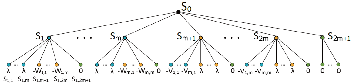
Figure 2: The MDP $\mathcal{M}$ constructed in our reduction.

Formally, layered MDP $\mathcal{M}$ has episode length $H=3$ with initial state ${\mathcal{S}}_{1}=\mathinner{\left\{S_{0}\right\}}$, $A$ states at the second time step denoted as ${\mathcal{S}}_{2}=\{S_{1},S_{2},\cdots S_{A}\}$, and $A^{2}$ states at the third time step denoted as ${\mathcal{S}}_{3}=\{S_{1,1},S_{1,2},\cdots S_{1,A},S_{2,1},\cdots,S_{A,A}\}$. We define state space ${\mathcal{S}}={\mathcal{S}}_{1}\cup{\mathcal{S}}_{2}\cup{\mathcal{S}}_{3}$. Define action space $\mathcal{A}=\{a_{1},a_{2},\cdots,a_{A}\}$, initial distribution $\rho(S_{0})=1$ and deterministic transition dynamics $P_{1}(S_{i}|S_{0},a_{i})=1$, $P_{2}(S_{i,j}|S_{i},a_{j})=1$ for all $i,j\in[A]$. Define cost function $c(s,a)\mathrel{\mathop{\mathchar 58\relax}}=\bar{c}(s)$, where

$$\bar{c}(s)\mathrel{\mathop{\mathchar 58\relax}}=\left\{\begin{array}[]{ll}0,&s\in{\mathcal{S}}_{1}\cup{\mathcal{S}}_{2}\\ 0,&s=S_{i,j},\text{where }i=A\text{ or }j=A\\ -V_{j,i},&s=S_{i,j},\text{where }i\in[m]+m,j\in[m]\\ -W_{i,j},&s=S_{i,j},\text{where }i\in[m],j\in[m]+m\\ \lambda,&\text{otherwise}\end{array}\right.$$

where we denote $[m]+m\mathrel{\mathop{\mathchar 58\relax}}=\{m+1,\cdots,2m\}$ and set $\lambda=54$.

On the policy side, we define benchmark policy class $\mathcal{B}$ that contains $A-1=2m$ deterministic policies $h_{j}$ ($j\in[A-1]$), such that $\forall s\in{\mathcal{S}}$, $h_{j}(s)=a_{j}$. Define deterministic expert policy $\pi^{E}$ as: $\pi^{E}(s)=a_{A}$, $\forall s\in{\mathcal{S}}$. Note that action $a_{A}$ is never a choice for policies in $\mathcal{B}$ but always chosen by the expert. Recall the mixed policy set $\Pi_{\mathcal{B}}$ is defined as

$$\Pi_{\mathcal{B}}\mathrel{\mathop{\mathchar 58\relax}}=\mathinner{\left\{\pi_{u}(\cdot|s)\mathrel{\mathop{\mathchar 58\relax}}=\sum_{h\in\mathcal{B}}u[h]\cdot h(\cdot|s)\mathrel{\mathop{\mathchar 58\relax}}u\in\Delta(\mathcal{B})\right\}}.$$

For the expert feedback function $\zeta_{E}$, we use advantage function $A^{E}(s,a)=Q_{\pi^{E}}(s,a)-V_{\pi^{E}}(s)$. The values of $A^{E}(s,a)$ are calculated as follows:

• For $s$ in ${\mathcal{S}}_{3}$: since for every $a$, $Q_{\pi^{E}}(s,a)=c(s,a)=\bar{c}(s)=0$, we have $A^{E}(s,a)=0$.

• For $s$ in ${\mathcal{S}}_{2}$:

  • First, suppose $s=S_{i}$ for $i\in\mathinner{\left\{1,\ldots,A-1\right\}}$. Following $\pi^{E}$ directs the agent to $S_{i,A}$, which encounters zero subsequent cost. This implies that $V_{\pi^{E}}(S_{i})=0$. On the other hand, taking action $a_{j}$ transitions to $S_{i,j}$ which encounters cost $\bar{c}(S_{i,j})$ subsequently. This means that $A^{E}(S_{i},a_{j})=\bar{c}(S_{i,j})$. Recall that $\forall i\in[A]$ $\bar{c}(S_{i,A})=0$, by this we have that $A^{E}(S_{i},a_{A})=0$ for all $S\in{\mathcal{S}}_{2}$.

  • Next, suppose s = $S_{A}$. Taking any action $a$ and following policy $\pi^{E}$ afterwards encounters zero subsequent cost, which implies that $Q_{\pi^{E}}(S_{A},a)=0$. This implies that $V_{\pi^{E}}(S_{A})=0$ and $A^{E}(S_{A},a)=0$.

• For $s$ in ${\mathcal{S}}_{1}$: at the initial state $S_{0}$, taking any action $a$ and following $\pi^{E}$ afterwards takes the agents to state $S_{i,A}$ for some $i$, which has zero cost. This implies that $Q_{\pi^{E}}(S_{A},a)=0$, $V_{\pi^{E}}(S_{A})=0$, and $A^{E}(S_{A},a)=0$.

In summary, we have

$$\zeta_{E}(s,a)\mathrel{\mathop{\mathchar 58\relax}}=A^{E}(s,a)=\left\{\begin{array}[]{ll}0,&s\in{\mathcal{S}}_{1}\cup{\mathcal{S}}_{3}\;\text{or}\;s=S_{A}\;\text{or}\;a=a_{A}\\ -V_{j,i},&s=S_{i},a=a_{j},\text{where }i\in[m]+m,j\in[m]\\ -W_{i,j},&s=S_{i},a=a_{j},\text{where }i\in[m],j\in[m]+m\\ \lambda,&\text{otherwise}\end{array}\right.$$

In summary, given any Poly¹²-Bimatrix instance $(U,V)$, f returns a Poly⁶-VI-MDP instance $(\mathcal{M},\zeta_{E},\mathcal{B})$.

Map g. The map g is defined as: given $u^{*}=(u^{*}_{x},u^{*}_{y})\in\Delta(\mathcal{B})$, return

$$\hat{x}=\frac{u^{*}_{x}}{\|u^{*}_{x}\|_{1}},\quad\hat{y}=\frac{u^{*}_{y}}{\|u^{*}_{y}\|_{1}}.$$

Polynomial-time computability of the reduction.

For map f, given any Poly¹²-Bimatrix instance $(V,W)$ with $V,W\in\mathbb{[}0,1]^{m\times m}$, map $\textsf{f}(V,W)$ returns $(\mathcal{M},\zeta_{E},\mathcal{B})$, where $\mathcal{M}=({\mathcal{S}},\mathcal{A},H,c,\rho,P)$ has $|{\mathcal{S}}|=(2m+1)^{2}+(2m+1)+1=O(m^{2})$ states, $|\mathcal{A}|=2m+1=O(m)$ actions, $H=3$, $|{\mathcal{S}}|\cdot|\mathcal{A}|=O(m^{3})$ cost function values, $(2m+2)(2m+1)=O(m^{2})$ values for the deterministic transition probability and one fixed initial distribution. Meanwhile, map f returns $2m$ deterministic benchmark policies and $\zeta_{E}$ function with $|{\mathcal{S}}|\cdot|\mathcal{A}|=O(m^{3})$ values. Combining the above, we conclude that f runs in $O(m^{3})$ time.

For map g, by its definition, it can be computed in $O(m)$ time. In all, f and g are computable in polynomial-time with respect to $m$.

Correctness of the reduction.

1. If $(V,W)$ is a valid input of Poly¹²-Bimatrix, then $V,W\in\mathbb{[}0,1]^{m\times m}$. Given any $V,W\in\mathbb{[}0,1]^{m\times m}$, by the definition of f, it is straightforward to see f constructs an discrete state-action episodic MDP with expert feedback $\zeta_{E}\mathrel{\mathop{\mathchar 58\relax}}{\mathcal{S}}\times\mathcal{A}\to\mathbb{R}$ and deterministic policy class $\mathcal{B}$. Thus, $\textsf{f}(V,W)$ is a valid input of Poly⁶-VI-MDP.

2. By Lemma 31 (given below), if $u^{*}$ is a solution of Poly⁶-VI-MDP instance $\textsf{f}(V,W)$, then $\textsf{g}(u^{*})$ is also a solution of Poly¹²-Bimatrix instance $(V,W)$.

3. By Lemma 29, any Poly⁶-VI-MDP instance has a solution.

In conclusion, Poly¹²-Bimatrix $\leq_{p}$ Poly⁶-VI-MDP, thus Poly⁶-VI-MDP is $\mathrm{PPAD}$-hard. ∎

Lemma 31.

$\textsf{g}(u^{*})$ is a solution of Poly¹²-Bimatrix instance $(V,W)$ if $u^{*}$ is a solution of Poly⁶-VI-MDP instance $\textsf{f}(V,W)$.

Proof.

Recall that $u^{*}$ the solution of a Poly⁶-VI-MDP instance $(\mathcal{M},\zeta_{E},\mathcal{B})$ satisfies $\forall u\in\Delta(\mathcal{B})$, $\left\langle\theta(u^{*}),u-u^{*}\right\rangle\geq-(S+A+B)^{-6}$, where $S=|{\mathcal{S}}|,A=|\mathcal{A}|,B=|\mathcal{B}|$. The proof follows by first calculating vector field $\theta(u)$ induced by $(\mathcal{M},\zeta_{E},\mathcal{B})$, and then showing that $\textsf{g}(u^{*})$ is a solution of the original Poly¹²-Bimatrix instance $(V,W)$ if $u^{*}$ is a solution of Poly⁶-VI-MDP instance $\textsf{f}(V,W)$.

To begin with, given $V,W\in[0,1]^{m\times m}$ we calculate $\theta$ in the Poly⁶-VI-MDP instance $\textsf{f}(V,W)$.

We have by definition in Section 3, $\forall u\in\Delta(\mathcal{B})$,

$$\theta(u)=\left(\mathbb{E}_{s\sim d_{\pi_{u}}}\mathbb{E}_{a\sim h_{j}(\cdot\mid s)}\left[\zeta_{E}(s,a)\right]\right)_{h_{j}\in\mathcal{B}}=\frac{1}{3}\left(\mathbb{E}_{s\sim d^{2}_{\pi_{u}}}\left[\zeta_{E}(s,h_{j}(s))\right]\right)_{h_{j}\in\mathcal{B}},$$

where in the second equality we recall that $d^{2}_{\pi_{u}}$ denotes the state occupancy distribution at the second step and $d_{\pi_{u}}=\frac{1}{3}(d^{1}_{\pi_{u}}+d^{2}_{\pi_{u}}+d^{3}_{\pi_{u}})$. The second equality is by the fact that $\zeta_{E}(s,a)$ is always $0$ when $s\in{\mathcal{S}}_{1}\cup{\mathcal{S}}_{3}$.

Recall that $h_{j}(s)=a_{j}$ and $B=2m$ as defined in the proof of Theorem 30, it can be verified that $\pi_{u}(\cdot|s)=\sum_{j\in[2m]}u[j]\cdot h_{j}(\cdot|s)=(u[1],u[2],\cdots,u[2m],0)^{\top}$ , where the last entry is $0$ since the last action is never chosen by any $h_{j}\in\mathcal{B}$. We can calculate its state occupancy distribution at step 2 as: $\mathrm{Pr}_{s\sim d^{2}_{\pi_{u}}}(s=S_{i})=u[i]$ for $i\in[2m]$ and $\mathrm{Pr}_{s\sim d^{2}_{\pi_{u}}}(s=S_{A})=0$. Therefore, $\forall j\in[2m]$,

$$\mathbb{E}_{s\sim d^{2}_{\pi_{u}}}\left[\zeta_{E}(s,a_{j})\right]=\sum_{i=1}^{2m}u[i]\zeta_{E}(S_{i},a_{j}).$$

For any $u\in\Delta(\mathcal{B})$, we use $u_{x},u_{y}$ to denote the vector that consists of the first $m$ elements and the last $m$ elements of $u$ respectively. Given $V,W\in[0,1]^{m\times m}$, define matrix

$$C\mathrel{\mathop{\mathchar 58\relax}}=\begin{pmatrix}\lambda{\bf 1}_{m\times m}&-V\\ -W^{\top}&\lambda{\bf 1}_{m\times m}\end{pmatrix}\in\mathbb{R}^{2m\times 2m},$$

where ${\bf 1}_{m\times m}$ denotes the matrix whose entries are all 1’s. Notice that by the value of $\zeta_{E}$ calculated in the proof of Theorem 30, it can be verified that $\forall i\in[2m],\forall j\in[2m]$, $\zeta_{E}(S_{i},a_{j})=C_{i,j}$. With this, $\theta(u)$ can be written in matrix form:

$$\theta(u)=\frac{1}{3}\left(\sum_{i=1}^{2m}u[i]\zeta_{E}(S_{i},a_{j})\right)_{j\in[2m]}=\frac{1}{3}\begin{pmatrix}\lambda{\bf 1}_{m\times m}&-V\\ -W^{\top}&\lambda{\bf 1}_{m\times m}\end{pmatrix}\cdot\begin{pmatrix}u_{x}\\ u_{y}\end{pmatrix}=\frac{1}{3}Cu.$$ (11)

Therefore, the constructed discrete state-action episodic MDP $\mathcal{M}$, expert feedback $\zeta_{E}$ and benchmark policy class $\mathcal{B}$ induces the following instance of Poly⁶-VI-MDP: find $u^{*}\in\Delta(\mathcal{B})$ such that $\forall u\in\Delta(\mathcal{B})$,

$$\left\langle\theta(u^{*}),u-u^{*}\right\rangle=\left\langle\frac{1}{3}Cu^{*},u-u^{*}\right\rangle\geq-(S+A+B)^{-6}=-(4m^{2}+10m+4)^{-6},$$ (12)

where we recall that $S=(2m+1)^{2}+(2m+1)+1$, $A=2m+1$, and $B=2m$.

Next, we show that $\textsf{g}(u^{*})$ is a solution of Poly¹²-Bimatrix instance $(V,W)$.

Recall that in Section F.1, given $V,W\in[0,1]^{m\times m}$, the mixed strategies on set $\mathcal{A}_{x}$ and sets $\mathcal{A}_{y}$ and $|\mathcal{A}_{x}|=|\mathcal{A}_{y}|=m$ are represented by $x\in\Delta(\mathcal{A}_{x})$ and $y\in\Delta(\mathcal{A}_{y})$, respectively. If $(\hat{x},\hat{y})\in\Delta(\mathcal{A}_{x})\times\Delta(\mathcal{A}_{y})$ is a solution of Poly¹²-Bimatrix instance $(V,W)$, then $(\hat{x},\hat{y})$ satisfies for any $x\in\Delta(\mathcal{A}_{x})$ and $y\in\Delta(\mathcal{A}_{y})$,

$$\left\{\begin{aligned} \hat{x}^{\top}V\hat{y}\geq x^{\top}V\hat{y}-m^{-12},\\ \hat{x}^{\top}W\hat{y}\geq\hat{x}^{\top}Wy-m^{-12}.\end{aligned}\right.$$

Now, consider $u^{*}=(u^{*}_{x},u^{*}_{y})\in\Delta(\mathcal{B})$, a solution for Poly⁶-VI-MDP instance $\textsf{f}(V,W)$, such that $\forall u\in\Delta(\mathcal{B})$,

$$\left\langle\theta(u^{*}),u-u^{*}\right\rangle\geq-(4m^{2}+10m+4)^{-6}=-\epsilon,$$

where we use $\epsilon$ to denote $(4m^{2}+10m+4)^{-6}$.

We will show that $(\hat{x},\hat{y})=\textsf{g}(u^{*})=(\frac{u_{x}^{*}}{\|u_{x}^{*}\|_{1}},\frac{u_{y}^{*}}{\|u_{y}^{*}\|_{1}})$ is a solution of Poly¹²-Bimatrix instance $(V,W)$. To see this, we first prove that $\forall x\in\Delta(\mathcal{A}_{x})$,

$${\hat{x}}^{\top}V\hat{y}\geq x^{\top}V\hat{y}-m^{-12}.$$ (13)

To this end, $\forall x\in\Delta(\mathcal{A}_{x})$, by setting $u=(\|u^{*}_{x}\|_{1}\cdot x,u^{*}_{y})\in\Delta(\mathcal{B})$ and plugging this choice of $u$ into Equation (12), we have

$$-\epsilon\leq \left\langle\frac{1}{3}Cu^{*},u-u^{*}\right\rangle$$

$$= \frac{\|u_{x}^{*}\|_{1}}{3}\begin{pmatrix}(x-\hat{x})^{\top},{\bf 0}^{\top}\end{pmatrix}\begin{pmatrix}\lambda{\bf 1}_{m\times m}&-V\\ -W^{\top}&\lambda{\bf 1}_{m\times m}\end{pmatrix}\cdot\begin{pmatrix}u_{x}^{*}\\ u_{y}^{*}\end{pmatrix}$$

$$= \frac{\|u_{x}^{*}\|_{1}}{3}\left(\lambda(x-\hat{x})^{\top}{\bf 1}_{m\times m}u_{x}^{*}-(x-\hat{x})^{\top}Vu_{y}^{*}\right)$$

$$= \frac{\lambda\|u_{x}^{*}\|_{1}}{3}{\bf 0}^{\top}u_{x}^{*}-\frac{\|u_{x}^{*}\|_{1}}{3}(x-\hat{x})^{\top}Vu_{y}^{*}$$

$$= -\frac{\|u_{x}^{*}\|_{1}\|u_{y}^{*}\|_{1}}{3}(x-\hat{x})^{\top}V\hat{y},$$

where we use ${\bf 0}$ to denote the all $0$ vector in $\mathbb{R}^{m}$. Combining $\|u_{x}^{*}\|_{1}\cdot\|u_{y}^{*}\|_{1}\geq\frac{2}{9}$ as shown later by Lemma 32, we obtain

$$x^{\top}V\hat{y}-\hat{x}^{\top}V\hat{y}\leq\frac{3}{\|u_{x}^{*}\|_{1}\|u_{y}^{*}\|_{1}}\epsilon\leq\frac{27}{2}\epsilon=\frac{27}{2(4m^{2}+10m+4)^{6}}\leq m^{-12}.$$

This establishes Equation (13). Using a symmetrical argument, for any $y\in\Delta(\mathcal{A}_{y})$, by taking $u=(u^{*}_{x},\|u^{*}_{y}\|_{1}\cdot y)$, we can also show that $\forall y\in\Delta(\mathcal{A}_{y})$,

$${\hat{x}}^{\top}W\hat{y}\geq\hat{x}^{\top}Wy-m^{-12}.$$ (14)

Combining Equations (13) and (14), we conclude that $(\hat{x},\hat{y})$ is a solution of Poly¹²-Bimatrix instance $(V,W)$. ∎

Lemma 32.

$\forall V,W\in[0,1]^{m\times m}$, if $u^{*}=(u_{x}^{*},u_{y}^{*})$ is a solution of Poly⁶-VI-MDP instance $\textsf{f}(V,W)$, then

$$\|u_{x}^{*}\|_{1}\cdot\|u_{y}^{*}\|_{1}\geq\frac{2}{9}.$$

Proof.

The lemma is proved by showing $\forall\;V,W\in[0,1]^{m\times m}$, $\forall u=(u_{x},u_{y})\in\Delta(\mathcal{B})$ such that $\|u_{x}\|_{1}\notin(\frac{1}{3},\frac{2}{3})$, for any $v=(v_{x},v_{y})\in\Delta(\mathcal{B})$ that satisfies $\|v_{x}\|_{1}=\|v_{y}\|_{1}=\frac{1}{2}$,

$$\left\langle\theta(u),v-u\right\rangle\leq-\frac{1}{3}<-(4m^{2}+10m+4)^{-6},$$

where we recall the definition of $\theta(\cdot)$ from Equation (11). This implies $u^{*}=(u^{*}_{x},u^{*}_{y})$ the solution of Poly⁶-VI-MDP instance $\textsf{f}(V,W)$ satisfies $\|u^{*}_{x}\|_{1},\|u^{*}_{x}\|_{1}\in[\frac{1}{3},\frac{2}{3}]$, $\forall\;V,W\in[0,1]^{m\times m}$. Finally, it can be easily verified that $\forall\;a,b\in[\frac{1}{3},\frac{2}{3}]$, $ab\geq\frac{2}{9}$.

By the alternative expression of $\theta(\cdot)$ shown in Equation (11), we can write $\left\langle\theta(u),u\right\rangle$ and $\left\langle\theta(u),v\right\rangle$ with $u=(u_{x},u_{y})$ and $v=(v_{x},v_{y})$ as:

$$\left\langle\theta(u),u\right\rangle= \frac{1}{3}(-u_{x}^{\top}Vu_{y}-u_{x}^{\top}Wu_{y}+\lambda(\|u_{x}\|_{1}^{2}+\|u_{y}\|_{1}^{2})),$$

$$\left\langle\theta(u),v\right\rangle= \frac{1}{3}(-v_{x}^{\top}Vu_{y}-u_{x}^{\top}Wv_{y}+\lambda(\|u_{x}\|_{1}\|v_{x}\|_{1}+\|u_{y}\|_{1}\|v_{y}\|_{1})).$$

By algebra, $\forall\;x\in\Delta(\mathcal{A}_{x})$, $\forall\;y\in\Delta(\mathcal{A}_{y})$ for $|\mathcal{A}_{x}|=|\mathcal{A}_{y}|=m$, $\forall\;V,W\in[0,1]^{m\times m}$, $0\leq x^{\top}Vy,\;x^{\top}Wy\leq 1$, then

$$\left\langle\theta(u),v-u\right\rangle= \frac{1}{3}\left(u_{x}^{\top}Vu_{y}+u_{x}^{\top}Wu_{y}-v_{x}^{\top}Vu_{y}-u_{x}^{\top}Wv_{y}\right)$$

$$+\frac{1}{3}\left(\lambda\|u_{x}\|_{1}(\|v_{x}\|_{1}-\|u_{x}\|_{1})+\lambda\|u_{y}\|_{1}(\|v_{y}\|_{1}-\|u_{y}\|_{1})\right)$$

$$\leq \frac{2}{3}+18\left(\|u_{x}\|_{1}(\|v_{x}\|_{1}-\|u_{x}\|_{1})+\|u_{y}\|_{1}(\|v_{y}\|_{1}-\|u_{y}\|_{1})\right),$$

where we recall that $\lambda=54$. Therefore, consider $\|u_{x}\|\notin(\frac{1}{3},\frac{2}{3})$ and any $v$ such that $\|v_{x}\|=\|v_{y}\|=\frac{1}{2}$, we have:

$$\|u_{x}\|_{1}(\|v_{x}\|_{1}-\|u_{x}\|_{1})+\|u_{y}\|_{1}(\|v_{y}\|_{1}-\|u_{y}\|_{1})$$

$$= \|u_{x}\|_{1}(\frac{1}{2}-\|u_{x}\|_{1})+\|u_{y}\|_{1}(\frac{1}{2}-\|u_{y}\|_{1})$$

$$= -2(\|u_{x}\|_{1}-\frac{1}{2})^{2}<-\frac{1}{18}.$$

Plugging this back, we conclude that $\forall u=(u_{x},u_{y})\in\Delta(\mathcal{B})$ such that $\|u_{x}\|\notin(\frac{1}{3},\frac{2}{3})$, for any $v=(v_{x},v_{y})\in\Delta(\mathcal{B})$ such that $\|v_{x}\|=\|v_{y}\|=\frac{1}{2}$,

$$\left\langle\theta(u),v-u\right\rangle\leq\frac{2}{3}-1=-\frac{1}{3}.\qed$$

F.4 Computational hardness of achieving sublinear dynamic regret in Logger

Theorem 33 (Restatement of Theorem 12).

Fix $\gamma>0$, if there exist a COIL algorithm such that for any $\mathcal{M}$ and expert $\pi^{E}$, it interacts with $\mathcal{M}$, CSC oracle $\mathcal{O}$, expert feedback $\zeta_{E}(s,a)=A^{E}(s,a)$, and outputs a sequence of $\mathinner{\left\{\pi_{u_{n}}\right\}}_{n=1}^{N}\in\Pi_{\mathcal{B}}$ such that with probability at least $\frac{1}{2}$,

$$\mathrm{DReg}_{N}(\mathcal{B})\leq O(\mathrm{poly}(S,A,B)\cdot N^{1-\gamma}),$$

in $\mathrm{poly}(N,S,A,B)$ time, then all problems in $\mathrm{PPAD}$ are solvable in randomized polynomial time.

Proof.

We start the proof by showing if there exists a COIL algorithm Alg1 that achieves $p(S,A,B)N^{1-\gamma}$ dynamic regret with probability $\frac{1}{2}$ in time $q(N,S,A,B)$, where $p$ and $q$ are polynomial functions, then, Alg1 yields an algorithm $\textsf{Alg1}^{\prime}$ (Algorithm 5) that solves Poly⁶-VI-MDP with expected polynomial time $\mathrm{poly}(S,A,B)$.

Algorithm 5 $\textsf{Alg1}^{\prime}$

1:  while true do

2:     Run Alg1 on $\mathcal{M}$, $\mathcal{B}$, $\zeta_{E}$, $\mathcal{O}$ for $N=(p(S,A,B)\cdot(S+A+B)^{6})^{\frac{1}{\gamma}}$ rounds, obtaining a sequence of policies $\mathinner{\left\{\pi_{n}\right\}}_{n=1}^{N}$ parameterized by $\mathinner{\left\{u_{n}\right\}}_{n=1}^{N}$.

3:     If any of $u_{n}$ is a $(S+A+B)^{-6}$-approximate solution of $\textsc{VI}(\Delta(\mathcal{B}),\theta)$, return $u_{n}$.

4:  end while

Correctness.

As $\textsf{Alg1}^{\prime}$ return only if $u_{n}$ is an $(S+A+B)^{-6}$-approximate solution of $\textsc{VI}(\Delta(\mathcal{B}),\theta)$, it solves the Poly⁶-VI-MDP problem.

Time complexity.

We now bound the time complexity of $\textsf{Alg1}^{\prime}$. Note that $\textsf{Alg1}^{\prime}$ sets Alg1 with $N=(p(S,A,B)\cdot(S+A+B)^{6})^{\frac{1}{\gamma}}=\mathrm{poly}(S+A+B)$, and Alg1 has a running time of $\mathrm{poly}(N,S,A,B)=\mathrm{poly}(S,A,B)$, together, each iteration of $\textsf{Alg1}^{\prime}$ takes $\mathrm{poly}(S,A,B)$ time.

We now show that $\textsf{Alg1}^{\prime}$ runs for an expected number of iterations at most a constant. Specifically, the guarantees of Alg1 implies that for each iteration, with probability at least $\frac{1}{2}$,

$$\mathrm{DReg}_{N}(\mathcal{B})(\mathinner{\left\{\pi_{u_{n}}\right\}}_{n=1}^{N})= \sum_{n=1}^{N}F_{n}(\pi_{u_{n}})-\min_{\pi\in\mathcal{B}}F_{n}(\pi)$$

$$= \sum_{n=1}^{N}\left\langle\theta(u_{n}),u_{n}\right\rangle-\min_{u\in\Delta(\mathcal{B})}\left\langle\theta(u_{n}),u\right\rangle$$

$$= \sum_{n=1}^{N}\max_{u\in\Delta(\mathcal{B})}\left\langle\theta(u_{n}),u_{n}-u\right\rangle$$

$$\leq f(S,A,B)\cdot N^{1-\gamma},$$

where the first equality is from the definition of dynamic regret in Section 2, and the second is by $F_{n}(\pi_{u})=\left\langle\theta(u_{n}),u\right\rangle$. In this event, since $N=(p(S,A,B)\cdot(S+A+B)^{6})^{\frac{1}{\gamma}}$, we have that $\exists n\in[N]$ s.t.

$$\max_{u\in\Delta(\mathcal{B})}\left\langle\theta(u_{n}),u_{n}-u\right\rangle\leq p(S,A,B)\cdot N^{-\gamma}=(S+A+B)^{-6},$$

which means $u_{n}$ is a solution of Poly⁶-VI-MDP instance $(\mathcal{M},\zeta_{E},\mathcal{B})$. Hence, the expected number of iterations of running Alg1 before a valid solution being returned is smaller or equal to $\sum_{t=0}^{\infty}\left(\frac{1}{2}\right)^{t}=2$. Thus, the expected running time of $\textsf{Alg1}^{\prime}$ is $O(\mathrm{poly}(S+A+B))$.

By Theorem 30, all problems in $\mathrm{PPAD}$ are polynomial-time reducible to Poly⁶-VI-MDP. If there exist a COIL algorithm Alg1 that achieves sublinear dynamic regret in Logger, then $\textsf{Alg1}^{\prime}$ can be constructed to solve Poly⁶-VI-MDP in randomized polynomial time, which means all problems in $\mathrm{PPAD}$ are solvable in randomized polynomial time. ∎

Appendix G Online linear optimization results

In this section, we first provide a recap on online linear optimization, the well-known Optimistic Follow the Regularized Leader (FTRL) algorithm (Algorithm 6) rakhlin2013online , and its regret guarantees (Theorem 42). Section G.3 instantiates this general result with the regularizer $R_{\mathcal{N}}$ (Equation (5)) defined in Section E.1.

G.1 Basic facts on convex analysis

Before we delve into the optimistic FTRL algorithm, we state some useful definitions and facts from convex analysis.

Definition 34.

For a differentiable convex function $f\mathrel{\mathop{\mathchar 58\relax}}\mathbb{R}^{d}\to\mathbb{R}$, define $D_{f}(v,w)=f(v)-f(w)-\left\langle v-w,\nabla f(w)\right\rangle$ to be the Bregman divergence induced by $f$.

Definition 35.

Given a convex function $f\mathrel{\mathop{\mathchar 58\relax}}\mathbb{R}^{d}\to\mathbb{R}\cup\mathinner{\left\{+\infty\right\}}$, where $\Omega\subseteq\mathbb{R}^{d}$, define $f^{*}\mathrel{\mathop{\mathchar 58\relax}}\mathbb{R}^{d}\to\mathbb{R}\cup\mathinner{\left\{+\infty\right\}}$ as $f^{*}(\theta)\mathrel{\mathop{\mathchar 58\relax}}=\sup_{w\in\mathbb{R}^{d}}\left(\left\langle\theta,w\right\rangle-f(w)\right)$ to be its Fechel conjugate.

Definition 36.

A convex function $f\mathrel{\mathop{\mathchar 58\relax}}\mathbb{R}^{d}\to\mathbb{R}\cup\mathinner{\left\{+\infty\right\}}$ is proper if it is not identically equal to $+\infty$.

Definition 37.

A function $f\mathrel{\mathop{\mathchar 58\relax}}\mathbb{R}^{d}\rightarrow\mathbb{R}\cup\mathinner{\left\{+\infty\right\}}$ is $\alpha$-strongly convex w.r.t. a norm $\|\cdot\|$ if for all $v,w$ in the relative interior of the effective domain of $f$ and $\lambda\in(0,1)$ we have

$$f(\lambda v+(1-\lambda)w)\leq\lambda f(v)+(1-\lambda)f(w)-\frac{1}{2}\alpha\lambda(1-\lambda)\|v-w\|^{2}.$$

Definition 38.

A function $f\mathrel{\mathop{\mathchar 58\relax}}\mathbb{R}^{d}\rightarrow\mathbb{R}$ is $\beta$-strongly smooth w.r.t. a norm $\|\cdot\|$ if $f$ is everywhere differentiable and if for all $v,w\in\mathbb{R}^{d}$ we have

$$f(v+w)\leq f(v)+\langle\nabla f(v),w\rangle+\frac{1}{2}\beta\|w\|^{2}.$$

Definition 39.

For a convex function $f\mathrel{\mathop{\mathchar 58\relax}}\mathbb{R}^{d}\to\mathbb{R}\cup\mathinner{\left\{+\infty\right\}}$, define its effective domain $\mathrm{dom}(f)\mathrel{\mathop{\mathchar 58\relax}}=\mathinner{\left\{w\in\mathbb{R}^{d}\mathrel{\mathop{\mathchar 58\relax}}f(w)<+\infty\right\}}$.

Note that the effective domain of a strongly smooth function $f$ satisfies $\mathrm{dom}(f)=\mathbb{R}^{d}$.

Fact 40.

Let $f\mathrel{\mathop{\mathchar 58\relax}}\mathbb{R}^{d}\to\mathbb{R}\cup\mathinner{\left\{+\infty\right\}}$ be a proper, closed and convex function, then:

1. $f^{*}$ is closed and convex (rockafellar1970convex [Theorem 12.2]);

2. $f^{**}=f$ (rockafellar1970convex [Corollary 12.2.1]);

3. $\theta\in\partial f(w)\Leftrightarrow f(w)+f^{*}(\theta)=\left\langle\theta,w\right\rangle\Leftrightarrow w\in\partial f^{*}(\theta)$, where $\partial g(w)$ denotes $g$’s subdifferential set at $w$ (zalinescu2002convex [Theorem 2.4.2]);

4. $f$ is $\alpha$-strongly convex with respect to a norm $\|\cdot\|$ if and only if $f^{\star}$ is $\frac{1}{\alpha}$-strongly smooth with respect to the dual norm $\|\cdot\|_{\star}$ (kakade2012regularization [Theorem 3]).

Proposition 41.

Let $f\mathrel{\mathop{\mathchar 58\relax}}\mathbb{R}^{d}\rightarrow\mathbb{R}\cup\mathinner{\left\{+\infty\right\}}$ be proper, closed and $\alpha$-strongly convex with respect to $\|\cdot\|$, then $f^{*}$ is differentiable, and $\nabla f^{*}(\theta)=\mathop{\mathrm{argmax}}_{w\in\mathrm{dom}(f)}\left(\left\langle\theta,w\right\rangle-f(w)\right).$

Proof sketch.

Given a function $f$ that is proper, closed and strongly convex, define $f_{1}\mathrel{\mathop{\mathchar 58\relax}}\mathrm{dom}(f)\to\mathbb{R}$, where $f_{1}(w)\mathrel{\mathop{\mathchar 58\relax}}=f(w)$ on $\mathrm{dom}(f)$. It can be seen that $f_{1}\mathrel{\mathop{\mathchar 58\relax}}\Omega\rightarrow\mathbb{R}$ is closed and strongly convex. It can be checked that $f^{*}(\theta)=\sup_{w\in\mathbb{R}^{d}}\left(\left\langle\theta,w\right\rangle-f(w)\right)=\sup_{w\in\mathrm{dom}(f)}\left(\left\langle\theta,w\right\rangle-f(w)\right)=f_{1}^{*}(\theta)$ where $f_{1}^{*}$ is defined using the notations in shalev2007online . The proposition follows from  shalev2007online [Lemma 15]. ∎

G.2 General results on FTRL and Optimistic FTRL

Online linear optimization refers to the following $N$-round protocol: the learner is given a convex decision set $\Omega\subset\mathbb{R}^{d}$. At every round $n\in[N]$, the learner chooses some decision $u_{n}\in\Omega$, and then receives a linear loss $\left\langle g_{n},\cdot\right\rangle$, where $g_{n}\in\mathbb{R}^{d}$. The goal of the learner is to minimize its regret on this sequence of linear losses:

$$\mathrm{LReg}_{N}\mathrel{\mathop{\mathchar 58\relax}}=\sum_{n=1}^{N}\left\langle g_{n},u_{n}\right\rangle-\min_{u\in\Omega}\sum_{n=1}^{N}\left\langle g_{n},u\right\rangle.$$

Optimistic FTRL (Algorithm 6), works for online linear optimization with a general decision set $\Omega$. It takes into input a strongly convex regularizer $R$ with effective domain $\Omega$ and a learning rate $\eta>0$. It maintains the cumulative linear loss $\Theta_{n}=\sum_{i=1}^{n}g_{i}$ over time (line 6); at round $n$, it first uses a predicted instantaneous loss $\hat{g}_{n}$ to construct a guess on the cumulative loss $\hat{\Theta}_{n}$ (line 3), then chooses the decision $u_{n}$ that minimizes the regularized guessed cumulative linear loss $\eta\langle\hat{\Theta}_{n},{u}\rangle+R(u)$ (line 4), which by Proposition 41, has an equivalent form of $\nabla R^{*}(-\eta\hat{\Theta}_{n})$. We have the following guarantee on the regret of Optimistic FTRL; it is largely inspired by and slightly generalizes the results of shalev2011online ; abernethy2014online ; rakhlin2013online .

0:  Convex decision set $\Omega\subseteq\mathbb{R}^{d}$, regularizer $R$ that is closed and $\alpha$-strongly convex with bounded $\mathrm{dom}(R)=\Omega$, learning rate $\eta>0$.

1:  Initialize $\Theta_{0}=0$.

2:  for $n=1,2,\ldots,N$ do

3:     The learner makes prediction $\hat{g}_{n}$, $\hat{\Theta}_{n}=\Theta_{n-1}+\hat{g}_{n}$ .

4:     The learner plays $u_{n}=\mathop{\mathrm{argmin}}_{u\in\Omega}\left(\eta\langle\hat{\Theta}_{n},{u}\rangle+R(u)\right)=\nabla R^{*}(-\eta\hat{\Theta}_{n})$ .

5:     The learner receives real loss $g_{n}$.

6:     Update $\Theta_{n}=\Theta_{n-1}+g_{n}$ .

7:  end for

Algorithm 6 Optimistic FTRL

Theorem 42.

Let $R\mathrel{\mathop{\mathchar 58\relax}}\mathbb{R}^{d}\rightarrow\mathbb{R}\cup\mathinner{\left\{+\infty\right\}}$ be a closed and $\alpha$-strongly convex function with respect to $\|\cdot\|$, such that $\Omega=\mathrm{dom}(R)$. The linear regret of Optimistic FTRL with $R$ and learning rate $\eta>0$, satisfies the following:

$$\mathrm{LReg}_{N}\leq \frac{\sup_{w\in\Omega}R(w)-\inf_{w\in\Omega}R(w)}{\eta}+\frac{1}{\eta}\sum_{n=1}^{N}\left(\underbrace{D_{R^{*}}\left(-\eta\Theta_{n},-\eta\hat{\Theta}_{n}\right)}_{\text{divergence penalty}}-\underbrace{D_{R^{*}}\left(-\eta\Theta_{n-1},-\eta\hat{\Theta}_{n}\right)}_{\text{prediction gain}}\right)$$ (15)

$$\leq \frac{\sup_{w\in\Omega}R(w)-\inf_{w\in\Omega}R(w)}{\eta}+\sum_{n=1}^{N}\frac{\eta\|\hat{g}_{n}-g_{n}\|_{*}^{2}}{2\alpha}-\frac{\alpha}{2\eta}\|\nabla R^{*}(-\eta\Theta_{n-1})-\nabla R^{*}(-\eta\hat{\Theta}_{n})\|^{2}.$$ (16)

Specifically, if $\hat{g}_{n}=0$ for all $n$,

$$\mathrm{LReg}_{N}\leq\frac{\sup_{w\in\Omega}R(w)-\inf_{w\in\Omega}R(w)}{\eta}+\sum_{n=1}^{N}\frac{\eta\|g_{n}\|_{*}^{2}}{2\alpha}.$$

Proof.

By the definition of Bregman divergence, we have

$$\left\{\begin{aligned} D_{R^{*}}(-\eta\Theta_{n},-\eta\hat{\Theta}_{n})&=R^{*}(-\eta\Theta_{n})-R^{*}(-\eta\hat{\Theta}_{n})-\left\langle-\eta\Theta_{n}+\eta\hat{\Theta}_{n},\nabla R^{*}(-\eta\hat{\Theta}_{n})\right\rangle,\\ D_{R^{*}}(-\eta\Theta_{n-1},-\eta\hat{\Theta}_{n})&=R^{*}(-\eta\Theta_{n-1})-R^{*}(-\eta\hat{\Theta}_{n})-\left\langle-\eta\Theta_{n-1}+\eta\hat{\Theta}_{n},\nabla R^{*}(-\eta\hat{\Theta}_{n})\right\rangle.\end{aligned}\right.$$

By rearranging the terms, the two equations can be rewritten as

$$\left\{\begin{aligned} \left\langle\eta\Theta_{n}-\eta\hat{\Theta}_{n},\nabla R^{*}(-\eta\hat{\Theta}_{n})\right\rangle&=-R^{*}(-\eta\Theta_{n})+R^{*}(-\eta\hat{\Theta}_{n})+D_{R^{*}}(-\eta\Theta_{n},-\eta\hat{\Theta}_{n}),\\ -\left\langle\eta\Theta_{n-1}-\eta\hat{\Theta}_{n},\nabla R^{*}(-\eta\hat{\Theta}_{n})\right\rangle&=R^{*}(-\eta\Theta_{n-1})-R^{*}(-\eta\hat{\Theta}_{n})-D_{R^{*}}(-\eta\Theta_{n-1},-\eta\hat{\Theta}_{n}).\end{aligned}\right.$$

By adding the two equations and recall that $\Theta_{n}=\Theta_{n-1}+g_{n}$ and $u_{n}=\nabla R^{*}(-\hat{\Theta}_{n})$, we can write

$$\eta\left\langle g_{n},u_{n}\right\rangle= \left\langle\eta\Theta_{n}-\eta\Theta_{n-1},\nabla R^{*}(-\eta\hat{\Theta}_{n})\right\rangle$$

$$= R^{*}(-\eta\Theta_{n-1})-R^{*}(-\eta\Theta_{n})+D_{R^{*}}(-\eta\Theta_{n},-\eta\hat{\Theta}_{n})-D_{R^{*}}(-\eta\Theta_{n-1},-\eta\hat{\Theta}_{n}).$$

Summing over $n=1,\ldots,N$, we have

$$\eta\sum_{n=1}^{N}\left\langle g_{n},u_{n}\right\rangle=R^{*}(0)-R^{*}(-\eta\Theta_{N})+\sum_{n=1}^{N}\left(D_{R^{*}}(-\eta\Theta_{n},-\eta\hat{\Theta}_{n})-D_{R^{*}}(-\eta\Theta_{n-1},-\eta\hat{\Theta}_{n})\right).$$

Therefore, we can bound $\eta\mathrm{LReg}_{N}$ as:

$$\eta\mathrm{LReg}_{N}=\sum_{n=1}^{N}\eta\left\langle g_{n},u_{n}\right\rangle-\min_{u\in\Omega}\sum_{n=1}^{N}\left\langle\eta g_{n},u\right\rangle$$

$$=-\min_{u\in\Omega}\left\langle\eta\Theta_{N},u\right\rangle+R^{*}(0)-R^{*}(-\eta\Theta_{N})+\sum_{n=1}^{N}\left(D_{R^{*}}(-\eta\Theta_{n},-\eta\hat{\Theta}_{n})-D_{R^{*}}(-\eta\Theta_{n-1},-\eta\hat{\Theta}_{n})\right)$$

$$=\max_{u\in\Omega}\left\langle-\eta\Theta_{N},u\right\rangle-R^{*}(-\eta\Theta_{N})+R^{*}(0)+\sum_{n=1}^{N}\left(D_{R^{*}}(-\eta\Theta_{n},-\eta\hat{\Theta}_{n})-D_{R^{*}}(-\eta\Theta_{n-1},-\eta\hat{\Theta}_{n})\right)$$

$$\leq\sup_{u\in\Omega}R(u)-\inf_{u\in\Omega}R(u)+\sum_{n=1}^{N}(D_{R^{*}}(-\eta\Theta_{n},-\eta\hat{\Theta}_{n})-D_{R^{*}}(-\eta\Theta_{n-1},-\eta\hat{\Theta}_{n})),$$

where the last inequality is by applying the definition of Fenchel conjugate and item 2 of Fact40:

1. $\max_{u\in\Omega}\left\langle-\eta\Theta_{N},u\right\rangle-R^{*}(-\eta\Theta_{N})\leq\sup_{u\in\Omega}\left(\sup_{\tilde{\Theta}\in\mathbb{R}^{d}}\left\langle-\tilde{\Theta},u\right\rangle-R^{*}(\tilde{\Theta})\right)=\sup_{u\in\Omega}R^{**}(u)=\sup_{u\in\Omega}R(u).$

2. $R^{*}(0)=\sup_{u\in\mathbb{R}^{d}}\left\langle 0,u\right\rangle-R(u)=\sup_{u\in\Omega}\left\langle 0,u\right\rangle-R(u)=-\inf_{u\in\Omega}R(u).$

This concludes the proof of Equation (15). We next prove Equation (16).

Upper bounding the divergence penalty terms $D_{R^{*}}(-\eta\Theta_{n},-\eta\hat{\Theta}_{n})$.

Since $R$ is closed and $\alpha$-strongly convex, by item 4 of Fact 40, $R^{*}$ is $\frac{1}{\alpha}$-strongly smooth and $\forall\Theta,\Theta^{\prime}\in\mathbb{R}^{d}$, $D_{R^{*}}(\Theta,\Theta^{\prime})\leq\frac{1}{2\alpha}\|\Theta-\Theta^{\prime}\|^{2},$ which implies $\forall n\in[N]$,

$$D_{R^{*}}(-\eta\Theta_{n},-\eta\hat{\Theta}_{n})\leq\frac{1}{2\alpha}\|\eta\Theta_{n}-\eta\hat{\Theta}_{n}\|_{*}^{2}=\frac{\eta^{2}}{2\alpha}\|g_{n}-\hat{g}_{n}\|_{*}^{2},$$

where the last equality is from the definition of $\Theta_{n}=g_{n}+\Theta_{n-1}$ and $\hat{\Theta}_{n}=\hat{g}_{n}+\Theta_{n-1}$.

Lower bounding the prediction gain terms $D_{R^{*}}(-\eta\Theta_{n-1},-\eta\hat{\Theta}_{n})$.

Since $R$ is closed and $\alpha$-strongly convex, by Lemma 54, we have

$$D_{R^{*}}(-\eta\Theta_{n-1},-\eta\hat{\Theta}_{n}))\geq\frac{\alpha}{2}\|\nabla R^{*}(-\eta\Theta_{n-1})-\nabla R^{*}(-\eta\hat{\Theta}_{n})\|^{2}.$$

Finally, combining Equation (15) with the bounds on divergence penalty and prediction gain terms, Equation (16) is proved. ∎

Remark 43.

An alternative proof of this theorem can be done using the Stronger Follow the Leader Lemma cheng2019accelerating ; mcmahan2017survey .

G.3 Regularizer induced by example-based perturbations

In this section, we instantiate the Optimistic FTRL algorithm and regret guarantee in the previous section with a specific $R$ that appears in our MFTPL, MFTPL-EG algorithms. Recall that in these algorithms, we use samples in the separator set $X$ and assign cost vector $\ell_{x}\sim\mathcal{N}(0,I_{A})$ independently on each of them. As a result, we define $R$ in Equation (5) as the Fenchel conjugate of $\Phi_{\mathcal{N}}(\Theta)=\mathbb{E}_{\ell\sim\mathcal{N}(0,I_{XA})}\left[\mathop{\max}\limits_{u\in\Delta(\mathcal{B})}\left\langle\Theta+q(\ell),u\right\rangle\right]$; recall that $q(\ell)=(\sum_{x\in\mathcal{X}}\ell_{x}(h(x))_{h\in B}$ and $\ell=\left(\ell_{x}\right)_{x\in\mathcal{X}}$.

First, we prove several useful properties of $\Phi_{\mathcal{N}}$.

Lemma 44 (Restatement of Lemma 16).

$\Phi_{\mathcal{N}}(\Theta)$ is differentiable for any $\Theta\in\mathbb{R}^{B}$ and $\nabla\Phi_{\mathcal{N}}(\Theta)=\mathbb{E}_{\ell\sim\mathcal{N}(0,I_{XA})}\left[\mathop{\mathop{\mathrm{argmax}}}\limits_{u\in\Delta(\mathcal{B})}\left\langle\Theta+q(\ell),u\right\rangle\right]$.

Proof.

To prove the lemma, by bertsekas1973stochastic [Propositions 2.2, 2.3], it suffices to prove that for any $\Theta$, $\mathop{\mathrm{argmax}}_{u\in\Delta(\mathcal{B})}\left\langle\Theta+q,u\right\rangle$ is unique with probability $1$, over the draw of $\ell\sim\mathcal{N}(0,I_{XA})$.

By the definition of $\mathop{\mathrm{argmax}}$, it can be seen that the solution of $\mathop{\mathop{\mathrm{argmax}}}\limits_{u\in\Delta(\mathcal{B})}\left\langle\Theta+q,u\right\rangle$ is not unique if and only if there exist $h,h^{\prime}\in\mathcal{B}$ and $h\neq h^{\prime}$, such that $\Theta[h]+q[h]=\Theta[h^{\prime}]+q[h^{\prime}]=\mathop{\max}\limits_{h}(\Theta[h]+q[h])$.

Define event $E=\mathinner{\left\{\mathop{\mathrm{argmax}}_{u\in\Delta(\mathcal{B})}\left\langle\Theta+q,u\right\rangle\text{is not unique}\right\}}$ and event $E_{hh^{\prime}}$: $\Theta[h]+q[h]=\Theta[h^{\prime}]+q[h^{\prime}]$, for all $h,h^{\prime}\in\mathcal{B}$ and $h\neq h^{\prime}$. For $E$ to happen, it is necessary that one of $E_{h,h^{\prime}}$ happens. Formally, $E\subseteq\mathop{\cup}\limits_{h\neq h^{\prime}}E_{hh^{\prime}}$. By applying the union bound, we obtain

$$\mathrm{Pr}(E)\leq\mathrm{Pr}(\mathop{\cup}\limits_{h\neq h^{\prime}}E_{hh^{\prime}})\leq\sum_{h\neq h^{\prime}}\mathrm{Pr}(E_{hh^{\prime}}).$$

We will now show that for any $h,h^{\prime}\in\mathcal{B}$ and $h\neq h^{\prime}$, $\Pr(E_{hh^{\prime}})=0$. By its definition , $E_{hh^{\prime}}$ happens if and only if $\Theta[h]+q[h]=\Theta[h^{\prime}]+q[h^{\prime}]$. We can rearrange the terms and get

$$q[h]-q[h^{\prime}]=\eta\cdot\left(\Theta[h]-\Theta[h^{\prime}]\right).$$

The following proof shows given any constant $C\in\mathbb{R}$, $q[h]-q[h^{\prime}]=C$ happens with probability 0. Here we first recall the definition of separator set $\mathcal{X}$: $\exists x\in\mathcal{X}$ s.t. $h(x)\neq h^{\prime}(x)$ for any $h\neq h^{\prime}$ and define $\mathcal{X}_{h,h^{\prime}}\mathrel{\mathop{\mathchar 58\relax}}=\mathinner{\left\{x\in\mathcal{X}|h(x)\neq h^{\prime}(x)\right\}}$. It can be seen that $\mathcal{X}_{h,h^{\prime}}$ is nonempty for $h\neq h^{\prime}$ by the definition of $\mathcal{X}$. Now we can rewrite $q[h]-q[h^{\prime}]$ with the help of $\mathcal{X}_{h,h^{\prime}}$,

$$q[h]-q[h^{\prime}]=\sum_{x\in\mathcal{X}}\ell_{x}(h(x))-\ell_{x}(h^{\prime}(x))=\sum_{x\in\mathcal{X}_{h,h^{\prime}}}\ell_{x}(h(x))-\ell_{x}(h^{\prime}(x)).$$

Since $\ell=\left(\ell_{x}\right)_{x\in\mathcal{X}}\sim\mathcal{N}(0,I_{XA})$, $q[h]-q[h^{\prime}]$ can be viewed as a sum of $2|\mathcal{X}_{h,h^{\prime}}|$ independent Gaussian variables following distribution $\mathcal{N}(0,1)$. By this observation, we have that $q[h]-q[h^{\prime}]\sim\mathcal{N}(0,4|\mathcal{X}_{h,h^{\prime}}|^{2})$, which implies $\forall C\in\mathbb{R}$, $\mathrm{Pr}(q[h]-q[h^{\prime}]=C)=0$. This in turn shows that $\Pr(E)\leq\sum_{h\neq h^{\prime}}\mathrm{Pr}(E_{hh^{\prime}})=0$, which concludes the proof of the lemma. ∎

Lemma 45.

$\Phi_{\mathcal{N}}$ is closed and convex on $\mathbb{R}^{B}$.

Proof.

To begin with, we show $\Phi_{\mathcal{N}}$ is convex. Recall that $\Phi_{\mathcal{N}}(\Theta)=\mathbb{E}_{\ell\sim\mathcal{N}(0,I_{XA})}\left[\mathop{\max}\limits_{u\in\Delta(\mathcal{B})}\left\langle\Theta+q(\ell),u\right\rangle\right]$ where $q(\ell)=(\sum_{x\in\mathcal{X}}\ell_{x}(h(x)))_{h\in B}$. To check the convexity of $\Phi_{\mathcal{N}}$, given any $\Theta,\Theta^{\prime}\in\mathbb{R}^{B}$ and any $\gamma\in[0,1]$, we have

$$\Phi_{\mathcal{N}}(\gamma\Theta+(1-\gamma)\Theta^{\prime})= \mathbb{E}_{\ell\sim\mathcal{N}(0,I_{XA})}\mathop{\max}\limits_{u\in\Delta(\mathcal{B})}\left\langle\gamma\Theta+(1-\gamma)\Theta^{\prime}+q(\ell),u\right\rangle$$

$$= \mathbb{E}_{\ell\sim\mathcal{N}(0,I_{XA})}\mathop{\max}\limits_{u\in\Delta(\mathcal{B})}\left\langle\gamma(\Theta+q(\ell))+(1-\gamma)(\Theta^{\prime}+q(\ell)),u\right\rangle$$

$$\leq \mathbb{E}_{\ell\sim\mathcal{N}(0,I_{XA})}(\mathop{\max}\limits_{u\in\Delta(\mathcal{B})}\left\langle\gamma(\Theta+q(\ell)),u\right\rangle+\mathop{\max}\limits_{u\in\Delta(\mathcal{B})}\left\langle(1-\gamma)(\Theta^{\prime}+q(\ell)),u\right\rangle$$

$$= \gamma\mathbb{E}_{\ell\sim\mathcal{N}(0,I_{XA})}\mathop{\max}\limits_{u\in\Delta(\mathcal{B})}\left\langle\Theta+q(\ell),u\right\rangle+(1-\gamma)\mathbb{E}_{\ell\sim\mathcal{N}(0,I_{XA})}\mathop{\max}\limits_{u\in\Delta(\mathcal{B})}\left\langle\Theta^{\prime}+q(\ell).u\right\rangle$$

$$= \gamma\Phi_{\mathcal{N}}(\Theta)+(1-\gamma)\Phi_{\mathcal{N}}(\Theta^{\prime}).$$

The inequality is by the fact that $\forall u\in\Delta(\mathcal{B})$, $\forall a,b\in\mathbb{R}^{B}$ , $\left\langle a+b,u\right\rangle\leq\mathop{\max}\limits_{u\in\Delta(\mathcal{B})}\left\langle a,u\right\rangle+\mathop{\max}\limits_{u\in\Delta(\mathcal{B})}\left\langle b,u\right\rangle$.

Secondly, to show $\Phi_{\mathcal{N}}$ is closed, by boyd2004convex [Section A.3.3], since $\mathbb{R}^{B}$ is closed, it suffice to show $\Phi_{\mathcal{N}}$ continuous on $\mathbb{R}^{B}$. Since $\Phi_{\mathcal{N}}$ is differentiable on $\mathbb{R}^{B}$ by Lemma 16, we have that $\Phi_{\mathcal{N}}$ is continuous, which concludes that $\Phi_{\mathcal{N}}$ is closed. ∎

The following two properties of $\Phi_{\mathcal{N}}$ are largely inspired by syrgkanis2016efficient .

Lemma 46.

$\Phi_{\mathcal{N}}(0)\leq\sqrt{2X\ln(B)}$.

Proof.

By the definition of $\Phi_{\mathcal{N}}$, we have $\Phi_{\mathcal{N}}(0)=\mathbb{E}_{\ell\sim\mathcal{N}(0,I_{XA})}\left[\mathop{\max}\limits_{u\in\Delta(\mathcal{B})}\left\langle q(\ell),u\right\rangle\right]$, where $q(\ell)=(\sum_{x\in\mathcal{X}}\ell_{x}(h(x)))_{h\in B}$. For the remainder of the proof, we use $\mathbb{E}$ as an abbreviation for $\mathbb{E}_{\ell\sim\mathcal{N}(0,I_{XA})}$. Recall that $q[h]=\sum_{x\in\mathcal{X}}\ell_{x}(h(x))$, we can write $\Phi_{\mathcal{N}}(0)=\mathbb{E}\left[\mathop{\max}\limits_{h\in\mathcal{B}}q[h]\right]$. For any $b>0$,

$$\exp\left(b\cdot\mathbb{E}\left[\mathop{\max}\limits_{h\in\mathcal{B}}q[h]\right]\right)\leq\mathbb{E}\left[\exp(b\cdot\mathop{\max}\limits_{h\in\mathcal{B}}q[h])\right]=\mathbb{E}\left[\mathop{\max}\limits_{h\in\mathcal{B}}\exp\left(b\cdot q[h]\right)\right]\leq\sum_{h\in\mathcal{B}}\mathbb{E}\left[\exp\left(b\cdot q[h]\right)\right],$$

where the first inequality is from the convexity of exponential function, while the last inequality is form $\mathop{\max}\limits_{h\in\mathcal{B}}\exp(bq[h])\leq\sum_{h\in\mathcal{B}}\exp(bq[h])$.

By the property of the sum of independent Gaussian variables, since $\ell\sim\mathcal{N}(0,I_{XA})$, we have that for any $h\in\mathcal{B}$, $q[h]=(\sum_{x\in\mathcal{X}}\ell_{x}(h(x)))_{h\in B}$ follows Gaussian distribution $\mathcal{N}(0,X)$. Then, $\forall h\in\mathcal{B}$, by a standard fact on the moment generating function of Gaussian random variables, we have that $\forall h\in\mathcal{B}$,

$$\mathbb{E}\exp(b\cdot q[h])=\exp\left(\frac{b^{2}X}{2}\right),$$

which implies

$$\exp\left(b\cdot\mathbb{E}\mathop{\max}\limits_{h\in\mathcal{B}}q[h]\right)\leq B\exp\left(\frac{b^{2}X}{2}\right).$$

Hence, by taking the natural logarithm and dividing by $b>0$ on both sides, we get

$$\mathbb{E}\left[\mathop{\max}\limits_{h\in\mathcal{B}}q[h]\right]\leq\frac{\ln(B)}{b}+\frac{bX}{2}.$$ (17)

Since Equation (17) holds for any $b>0$, by choosing $b=\sqrt{\frac{2\ln(B)}{X}}$, we obtain $\mathbb{E}\left[\mathop{\max}\limits_{h\in\mathcal{B}}q[h]\right]\leq\sqrt{2X\ln(B)}$, which concludes $\Phi_{\mathcal{N}}(0)\leq\sqrt{2X\ln(B)}$. ∎

Lemma 47.

$\Phi_{\mathcal{N}}$ is $\beta$-strongly smooth with respect to $\|\cdot\|_{\infty}$ with $\beta=\sqrt{\frac{8}{\pi}}AX$.

Proof.

To prove that $\Phi_{\mathcal{N}}$ is $\beta$-strongly smooth with respect to $\|\cdot\|_{\infty}$, by Definition 4.18 in orabona2019modern , it suffices to show that $\forall\Theta,\Theta^{\prime}\in\mathbb{R}^{B}$,

$$\|\nabla\Phi_{\mathcal{N}}(\Theta)-\nabla\Phi_{\mathcal{N}}(\Theta^{\prime})\|_{1}\leq\beta\|\Theta-\Theta^{\prime}\|_{\infty}.$$

By Lemma 16, $\nabla\Phi_{\mathcal{N}}(\Theta)=\mathbb{E}_{\ell\sim\mathcal{N}(0,I_{XA})}\left[\mathop{\mathop{\mathrm{argmax}}}\limits_{u\in\Delta(\mathcal{B})}\left\langle\Theta+q(\ell),u\right\rangle\right]$, where $q(\ell)=(\sum_{x\in\mathcal{X}}\ell_{x}(h(x)))_{h\in B}$. Given $\ell$, we introduce shorthands

$$u_{q}=\mathop{\mathop{\mathrm{argmax}}}\limits_{u\in\Delta(\mathcal{B})}\left\langle u,\Theta+q(\ell)\right\rangle,u^{\prime}_{q}=\mathop{\mathop{\mathrm{argmax}}}\limits_{u\in\Delta(\mathcal{B})}\left\langle u,\Theta^{\prime}+q(\ell)\right\rangle.$$

We also introduce the short hand $h_{q}$ and $h^{\prime}_{q}$ to represent the policy in class $\mathcal{B}$ selected by $u_{q}$ and $u^{\prime}_{q}$. More explicitly,

$$h_{q}=\mathop{\mathrm{argmax}}_{h\in B}\Theta[h]+q[h],\;\;h^{\prime}_{q}=\mathop{\mathrm{argmax}}_{h\in B}\Theta^{\prime}[h]+q[h].$$

By Lemma 16, $u_{q}$, $u^{\prime}_{q}$, $h_{q}$, $h_{q}^{\prime}$ are well-defined with probability $1$ over the randomness of $\ell$. With this notation, we have $\|u_{q}-u^{\prime}_{q}\|_{1}=0$ when $h_{q}=h^{\prime}_{q}$ , and $\|u_{q}-u^{\prime}_{q}\|_{1}=2$ when $h_{q}\neq h^{\prime}_{q}$, which means $\|u_{q}-u^{\prime}_{q}\|_{1}=2I(h_{q}\neq h^{\prime}_{q})$. From now on, we use $P(\ell)$ to denote the probability density function of $\ell$. By this, we have

$$\|\nabla\Phi_{\mathcal{N}}(\Theta)-\nabla\Phi_{\mathcal{N}}(\Theta^{\prime})\|_{1}= \|\mathbb{E}_{\ell\sim\mathcal{N}(0,I_{XA})}u_{q}-\mathbb{E}_{\ell\sim\mathcal{N}(0,I_{XA})}u^{\prime}_{q}\|_{1}$$

$$= \sum_{h\in\mathcal{B}}\left|\int_{\ell}(I(h=h_{q})-I(h=h^{\prime}_{q}))P(\ell)\operatorname{d\!}\ell\right|$$

$$\leq \sum_{h\in\mathcal{B}}\int_{\ell}\left|(I(h=h_{q})-I(h=h^{\prime}_{q}))\right|P(\ell)\operatorname{d\!}\ell$$

$$= \int_{\ell}\sum_{h\in\mathcal{B}}\left|(I(h=h_{q})-I(h=h^{\prime}_{q}))\right|P(\ell)\operatorname{d\!}\ell$$

$$= \int_{\ell}2I(h_{q}\neq h^{\prime}_{q})P(\ell)\operatorname{d\!}\ell$$

$$= 2\mathrm{Pr}(h_{q}\neq h^{\prime}_{q}),$$

where $\mathrm{Pr}(h_{q}\neq h^{\prime}_{q})$ denotes the probability of $h_{q}\neq h^{\prime}_{q}$ under the distribution of $\ell$. By the definition of separator set $\mathcal{X}$, $h\neq h^{\prime}$ if and only if $\exists x\in\mathcal{X}$ s.t. $h(x)\neq h^{\prime}(x)$. Then, by bringing in $h_{q},h^{\prime}_{q}$ and apply the union bound, we have

$$\mathrm{Pr}(h_{q}\neq h^{\prime}_{q})\leq\sum_{x\in\mathcal{X}}\mathrm{Pr}(h_{q}(x)\neq h^{\prime}_{q}(x))=\sum_{x\in\mathcal{X}}\sum_{a\in\mathcal{A}}\mathrm{Pr}(a=h_{q}(x)\neq h^{\prime}_{q}(x)).$$

Then, given any $x$ and $a$, we denote $\ell_{-xa}$ as all other Gaussian variables in set $\{\ell_{x}(a)\}_{x\in X,a\in\mathcal{A}}$ except $\ell_{x}(a)$ and $\mathrm{Pr}(a=h_{q}(x)\neq h^{\prime}_{q}(x))$ as the probability of $a=h_{q}(x)\neq h^{\prime}_{q}(x)$ under the distribution of $\ell_{-xa}$. Then, $\forall x\in X,a\in\mathcal{A}$,

$$\mathrm{Pr}(a=h_{q}(x)\neq h^{\prime}_{q}(x))=\int_{\ell_{-xa}}\mathrm{Pr}(a=h_{q}(x)\neq h^{\prime}_{q}(x)|\ell_{-xa})P(\ell_{-xa})d(\ell_{-xa}).$$

Conditioned on $\ell_{-xa}$, we denote $\tilde{\ell}=\{\tilde{\ell}_{x}(a)\}_{x\in X,a\in\mathcal{A}}$ as the corresponding perturbation vector that share the same value with $\ell$ on all other entries and set $\tilde{\ell}_{x}(a)=0$. Define

$$\Theta_{xa}=\Theta+\left(\sum_{x\in\mathcal{X}}\tilde{\ell}_{x}(h(x))\right)_{h\in\mathcal{B}},\;\;\Theta^{\prime}_{xa}=\Theta^{\prime}+\left(\sum_{x\in\mathcal{X}}\tilde{\ell}_{x}(h(x))\right)_{h\in\mathcal{B}}.$$

By algebra, $\Theta_{xa}-\Theta^{\prime}_{xa}=\Theta-\Theta^{\prime}$. By the definition of $u_{q}$ and $u^{\prime}_{q}$, with the new notation, we can rewrite

$$u_{q}=\mathop{\mathop{\mathrm{argmax}}}\limits_{u\in\Delta(\mathcal{B})}\left\langle u,\Theta_{xa}+(I(h(x)=a)\ell_{x}(a))_{h\in\mathcal{B}}\right\rangle,\;\;u^{\prime}(q)=\mathop{\mathop{\mathrm{argmax}}}\limits_{u\in\Delta(\mathcal{B})}\left\langle u,\Theta^{\prime}_{xa}+(I(h(x)=a)\ell_{x}(a))_{h\in\mathcal{B}}\right\rangle.$$

By using $(\Theta[h])_{h\in\mathcal{B}}\mathrel{\mathop{\mathchar 58\relax}}=\Theta$, we can write

$$h_{q}=\mathop{\mathop{\mathrm{argmax}}}\limits_{h\in\mathcal{B}}\Theta_{xa}[h]+I(h(x)=a)\ell_{x}(a),\;\;h^{\prime}_{q}=\mathop{\mathop{\mathrm{argmax}}}\limits_{h\in\mathcal{B}}\Theta^{\prime}_{xa}[h]+I(h(x)=a)\ell_{x}(a).$$

Then, by dividing the set $\mathcal{B}$ into disjoint subsets $\mathcal{B}_{xa}=\{h|h(x)=a,h\in\mathcal{B}\}$ and $\mathcal{B}\setminus\mathcal{B}_{xa}$. If $\mathcal{B}_{xa}=\varnothing$ or $\mathcal{B}\setminus\mathcal{B}_{xa}=\varnothing$ , we have that $\mathrm{Pr}(a=h_{q}(x)\neq h^{\prime}_{q}(x))=0$. Otherwise, we can view $h_{q}$ as the $h$ that corresponds to $\mathop{\max}\{\mathop{\max}\limits_{h\in\mathcal{B}_{xa}}\Theta_{xa}[h]+\ell_{x}(a),\mathop{\max}\limits_{h\in\mathcal{B}\setminus\mathcal{B}_{xa}}\Theta_{xa}[h]\}$, and $h^{\prime}_{q}$ as the $h$ that corresponds to $\mathop{\max}\{\mathop{\max}\limits_{h\in\mathcal{B}_{xa}}\Theta^{\prime}_{xa}[h]+\ell_{x}(a),\mathop{\max}\limits_{h\in\mathcal{B}\setminus\mathcal{B}_{xa}}\Theta^{\prime}_{xa}[h]\}$. With this insight, it can be seen that

$$\left\{\begin{aligned} \delta\mathrel{\mathop{\mathchar 58\relax}}=&\mathop{\max}\limits_{h\in\mathcal{B}\setminus\mathcal{B}_{xa}}\Theta_{xa}[h]-\mathop{\max}\limits_{h\in\mathcal{B}_{xa}}\Theta_{xa}[h]>\ell_{x}(a)\rightarrow a\neq h_{q}(x),\\ \delta^{\prime}\mathrel{\mathop{\mathchar 58\relax}}=&\mathop{\max}\limits_{h\in\mathcal{B}\setminus\mathcal{B}_{xa}}\Theta_{xa}^{\prime}[h]-\mathop{\max}\limits_{h\in\mathcal{B}_{xa}}\Theta_{xa}^{\prime}[h]<\ell_{x}(a)\rightarrow a=h^{\prime}_{q}(x).\end{aligned}\right.$$

Therefore, both $\delta\leq\ell_{x}(a)$ and $\ell_{x}(a)\leq\delta^{\prime}$ are necessary for $a=h_{q}(x)\neq h_{q}^{\prime}(x)$ to happen, which implies

$$\mathrm{Pr}(a=h_{q}(x)\neq h^{\prime}_{q}(x)|\ell_{-xa})\leq\mathrm{Pr}(\delta\leq\ell_{x}(a)\leq\delta^{\prime}).$$

If $\delta^{\prime}<\delta$, then $\mathrm{Pr}(a=h_{q}(x)\neq h^{\prime}_{q}(x)|\ell_{-xa})=0$. Otherwise ($\delta\leq\delta^{\prime}$), conditioned on $\ell_{-xa}$, by $\ell_{x}(a)\sim\mathcal{N}(0,1)$, we have

$$\mathrm{Pr}(a=h_{q}(x)\neq h^{\prime}_{q}(x)|\ell_{-xa},\delta^{\prime}\geq\delta)\leq\int_{\delta}^{\delta^{\prime}}\frac{1}{\sqrt{2\pi}}\exp(-\frac{\ell_{x}(a)^{2}}{2})\operatorname{d\!}(\ell_{x}(a))\leq\frac{1}{\sqrt{2\pi}}(\delta^{\prime}-\delta),$$

in which case,

$$\delta^{\prime}-\delta\leq \left|\mathop{\max}\limits_{h\in\mathcal{B}\setminus\mathcal{B}_{xa}}\Theta_{xa}[h]-\mathop{\max}\limits_{h\in\mathcal{B}\setminus\mathcal{B}_{xa}}\Theta\textquoteright_{xa}[h]\right|+\left|\mathop{\max}\limits_{h\in\mathcal{B}_{xa}}\Theta_{xa}[h]-\mathop{\max}\limits_{h\in\mathcal{B}_{xa}}\Theta^{\prime}_{xa}[h]\right|$$

$$\leq \left|\mathop{\max}\limits_{h\in\mathcal{B}}\Theta_{xa}[h]-\mathop{\max}\limits_{h\in\mathcal{B}}\Theta^{\prime}_{xa}[h]\right|+\left|\mathop{\max}\limits_{h\in\mathcal{B}}\Theta_{xa}[h]-\mathop{\max}\limits_{h\in\mathcal{B}}\Theta^{\prime}_{xa}[h]\right|$$

$$\leq 2\left|\mathop{\max}\limits_{h\in\mathcal{B}}(\Theta_{xa}[h]-\Theta^{\prime}_{xa}[h])\right|$$

$$\leq 2\mathop{\max}\limits_{h\in\mathcal{B}}\left|\Theta_{xa}[h]-\Theta^{\prime}_{xa}[h]\right|$$

$$= 2\|\Theta_{xa}-\Theta^{\prime}_{xa}\|_{\infty}=2\|\Theta-\Theta^{\prime}\|_{\infty}.$$

By this we conclude $\forall x\in\mathcal{X}$, $\forall a\in\mathcal{A}$, $\mathrm{Pr}(a=h_{q}(x)\neq h^{\prime}_{q}(x)|\ell_{-xa})\leq\sqrt{\frac{2}{\pi}}\|\Theta-\Theta^{\prime}\|_{\infty}$, and

$$\|\nabla\Phi_{\mathcal{N}}(\Theta)-\nabla\Phi_{\mathcal{N}}(\Theta^{\prime})\|_{1}\leq 2\sum_{x\in\mathcal{X}}\sum_{a\in\mathcal{A}}\mathrm{Pr}(a=h_{q}(x)\neq h^{\prime}_{q}(x))\leq\sqrt{\frac{8}{\pi}}AX\|\Theta-\Theta^{\prime}\|_{\infty}.\qed$$

Secondly, we prove useful properties of $R_{\mathcal{N}}\mathrel{\mathop{\mathchar 58\relax}}\mathbb{R}^{B}\to\mathbb{R}\cup\mathinner{\left\{+\infty\right\}}$, where $R_{\mathcal{N}}=\Phi_{\mathcal{N}}^{*}$.

Lemma 48 (Restatement of Lemma 17).

$R_{\mathcal{N}}(u)=\Phi_{\mathcal{N}}^{*}(u)$ is closed and $\sqrt{\frac{\pi}{8}}{\frac{1}{AX}}$-strongly convex with respect to $\|\cdot\|_{1}$.

Proof.

Since $\Phi_{\mathcal{N}}$ is closed and convex by Lemma 45, by item 1 of Fact 40, $R_{\mathcal{N}}(u)=\Phi_{\mathcal{N}}^{*}(u)$ is closed and convex. Also, by Lemma 47, $\Phi_{\mathcal{N}}$ is $\sqrt{\frac{8}{\pi}}AX$-strongly smooth with respect to $\|\cdot\|_{\infty}$. Then, we apply item 4 of Fact 40 and conclude $R_{\mathcal{N}}(u)$ is $\sqrt{\frac{\pi}{8}}{\frac{1}{AX}}$-strongly convex with respect to $\|\cdot\|_{1}$. ∎

Lemma 49.

$\forall u\in\Delta(\mathcal{B})$, $R_{\mathcal{N}}(u)\leq 0$.

Proof.

Recall that $R_{\mathcal{N}}(u)=\sup_{\Theta\in\mathbb{R}^{B}}\left\langle\Theta,u\right\rangle-\Phi_{\mathcal{N}}(\Theta)$, where $\Phi_{\mathcal{N}}(\Theta)=\mathbb{E}_{\ell\sim\mathcal{N}(0,I_{XA})}\left[\mathop{\max}\limits_{v\in\Delta(\mathcal{B})}\left\langle\Theta+q(\ell),v\right\rangle\right]$, it suffices to show $\forall u\in\Delta(\mathcal{B})$, $\forall\Theta\in\mathbb{R}^{B}$, $\left\langle\Theta,u\right\rangle-\Phi_{\mathcal{N}}(\Theta)\leq 0$. For the remainder of the proof, we use $\mathbb{E}$ as an abbreviation for $\mathbb{E}_{\ell\sim\mathcal{N}(0,I_{XA})}$. Then, $\forall u\in\Delta(\mathcal{B})$, $\forall\Theta\in\mathbb{R}^{B}$,

$$\Phi_{\mathcal{N}}(\Theta)=\mathbb{E}\left[\mathop{\max}\limits_{v\in\Delta(\mathcal{B})}\left\langle\Theta+q(\ell),v\right\rangle\right]\geq\mathop{\max}\limits_{v\in\Delta(\mathcal{B})}\mathbb{E}\left[\left\langle\Theta+q(\ell),v\right\rangle\right]=\mathop{\max}\limits_{v\in\Delta(\mathcal{B})}\left\langle\Theta,v\right\rangle\geq\left\langle\Theta,u\right\rangle,$$

where the first inequality is from Jensen’s inequality, while the second equality is by the fact that

$$\mathbb{E}\left[q(\ell)\right]=\mathbb{E}\left[(\sum_{x\in\mathcal{X}}\ell_{x}(h(x)))_{h\in\mathcal{B}}\right]=\sum_{x\in\mathcal{X}}\mathbb{E}\left[\ell_{x}(h(x))_{h\in\mathcal{B}}\right]=0.\qed$$

Lemma 50.

$\mathrm{dom}(R_{\mathcal{N}})=\Delta(\mathcal{B})$.

Proof.

We show the lemma in two steps. First, by Lemma 49, $\forall u\in\Delta(\mathcal{B})$, $R_{\mathcal{N}}(u)\leq 0$, which is finite. Secondly we show $\forall u\in\mathbb{R}^{B}\setminus\Delta(\mathcal{B})$, $R_{\mathcal{N}}(u)=+\infty$.

For the second step, $\forall u\in\mathbb{R}^{B}\setminus\Delta(\mathcal{B})$, by using $\mathbb{E}$ as an abbreviation for $\mathbb{E}_{\ell\sim\mathcal{N}(0,I_{XA})}$, we have

$$R_{\mathcal{N}}(u)= \sup_{\Theta\in\mathbb{R}^{B}}\left\langle\Theta,u\right\rangle-\Phi_{\mathcal{N}}(\Theta)$$

$$= \sup_{\Theta\in\mathbb{R}^{B}}\left\langle\Theta,u\right\rangle-\mathbb{E}\left[\mathop{\max}\limits_{v\in\Delta(\mathcal{B})}\left\langle\Theta+q(\ell),v\right\rangle\right]$$

$$\geq \sup_{\Theta\in\mathbb{R}^{B}}\left(\left\langle\Theta,u\right\rangle-\mathop{\max}\limits_{v\in\Delta(\mathcal{B})}\left\langle\Theta,v\right\rangle\right)-\mathbb{E}\left[\mathop{\max}\limits_{v^{\prime}\in\Delta(\mathcal{B})}\left\langle q(\ell),v^{\prime}\right\rangle\right],$$

where the first inequality is by the convexity of $\max$ and inner product functions.

By Lemma 46, $\Phi_{\mathcal{N}}(0)=\mathbb{E}\left[\mathop{\max}\limits_{v^{\prime}\in\Delta(\mathcal{B})}\left\langle q(\ell),v^{\prime}\right\rangle\right]\leq\sqrt{2X\ln(B)}$, which is a constant. Now, it suffices to show that $\forall u\in\mathbb{R}^{B}\setminus\Delta(\mathcal{B})$, $\sup_{\Theta\in\mathbb{R}^{B}}\left(\left\langle\Theta,u\right\rangle-\mathop{\max}\limits_{v\in\Delta(\mathcal{B})}\left\langle\Theta,v\right\rangle\right)=+\infty$.

We divide $\mathbb{R}^{B}\setminus\Delta(\mathcal{B})$ into two disjoint sets:

$$\left\{\begin{aligned} U^{-}\mathrel{\mathop{\mathchar 58\relax}}=&\{u\in\mathbb{R}^{B}\>|\>u[i]<0\>\text{for some}\>i\in\{1,2,\cdots,B\}\},\\ U^{+}\mathrel{\mathop{\mathchar 58\relax}}=&\{u\in\mathbb{R}^{B}\>|\>\|u\|_{1}>1,u\succeq 0\},\end{aligned}\right.$$

where it can be verified that $\mathbb{R}\setminus\Delta(\mathcal{B})=U^{-}\cup U^{+}$.

For any $u\in U^{-}$, where $u[i]<0$ for some $i\in\{1,2,\cdots,B\}$, we have that $\forall C\in\mathbb{R}$, by setting $\theta(u,i,C)=\frac{|C|+1}{u[i]}\operatorname{Onehot}(i,\mathcal{B})\in\mathbb{R}^{B}$,

$$\mathop{\max}\limits_{v\in\Delta(\mathcal{B})}\left\langle\theta(u,i,C),u-v\right\rangle= \left\langle\frac{|C|+1}{u[i]}\operatorname{Onehot}(i,\mathcal{B}),u\right\rangle-\mathop{\max}\limits_{v\in\Delta(\mathcal{B})}\left\langle\frac{|C|+1}{u[i]}\operatorname{Onehot}(i,\mathcal{B}),v\right\rangle$$

$$\geq \frac{|C|+1}{u[i]}\cdot u[i]=|C|+1>C,$$

where the first inequality is by $\left\langle\frac{|C|+1}{u[i]}\operatorname{Onehot}(i,\mathcal{B}),v\right\rangle\leq 0$, $\forall u[i]<0$, $\forall v\in\Delta(\mathcal{B})$. This implies $\forall u\in U^{-}$, $\sup_{\Theta\in\mathbb{R}^{B}}\left(\mathop{\max}\limits_{v\in\Delta(\mathcal{B})}\left\langle\Theta,u-v\right\rangle\right)=+\infty$. Thus, $\forall u\in U^{-}$, $R_{\mathcal{N}}(u)=+\infty$.

Similarly, for any $u\in U^{+}$, we have that $\forall C\in\mathbb{R}$, by setting $\theta(u,C)=\frac{|C|+1}{\|u\|_{1}-1}\cdot u\in\mathbb{R}^{B}$,

$$\mathop{\max}\limits_{v\in\Delta(\mathcal{B})}\left\langle\theta(u,C),u-v\right\rangle= \mathop{\max}\limits_{v\in\Delta(\mathcal{B})}\left\langle\frac{|C|+1}{\|u\|_{1}-1}\cdot u,u-v\right\rangle$$

$$= \left\langle\frac{|C|+1}{\|u\|_{1}-1}\cdot u,u-\frac{u}{\|u\|_{1}}\right\rangle$$

$$= \frac{|C|+1}{\|u\|_{1}-1}\cdot\|u\|_{1}\cdot(\|u\|_{1}-1)>C,$$

which is by basic algebra. This implies $\forall u\in U^{+}$, $R_{\mathcal{N}}(u)=+\infty$.

In conclusion, we have that $\forall u\in\mathbb{R}^{B}\setminus\Delta(\mathcal{B})=U^{-}\cup U^{+}$, $R_{\mathcal{N}}(u)=+\infty$, which concludes the the proof. ∎

Lemma 51 (Restatement of Lemma 18).

For any $\Theta\in\mathbb{R}^{d}$,

$$\mathop{\mathop{\mathrm{argmin}}}\limits_{u\in\Delta(\mathcal{B})}\left(\langle{\Theta},{u}\rangle+R_{\mathcal{N}}(u)\right)=\nabla\Phi_{\mathcal{N}}(-\Theta).$$

Proof.

As shown by Lemma 48 and Lemma 50, $R_{\mathcal{N}}$ is closed and strongly convex with $\mathrm{dom}(R_{\mathcal{N}})=\Delta(\mathcal{B})$. By applying Proposition 41 on $R_{\mathcal{N}}$, we have

$$\nabla R^{*}_{\mathcal{N}}(-\Theta)=\mathop{\mathop{\mathrm{argmax}}}\limits_{u\in\mathbb{R}^{B}}\left\langle-\Theta,u\right\rangle-R_{\mathcal{N}}(u)=\mathop{\mathop{\mathrm{argmin}}}\limits_{u\in\Delta(\mathcal{B})}\left\langle\Theta,u\right\rangle+R_{\mathcal{N}}(u),$$

where the second equality is by $\mathrm{dom}(R_{\mathcal{N}})=\Delta(\mathcal{B})$ shown in Lemma 50.

As shown by Lemma 45, $\Phi_{\mathcal{N}}$ is closed and convex. By item 2 of Fact 40, $R^{*}_{\mathcal{N}}=\Phi_{\mathcal{N}}^{**}=\Phi_{\mathcal{N}}$, which concludes the proof. ∎

Lemma 52.

$\sup_{u\in\Delta(\mathcal{B})}R_{\mathcal{N}}(u)-\inf_{u\in\Delta(\mathcal{B})}R_{\mathcal{N}}(u)\leq\sqrt{2X\ln(B)}.$

Proof.

First, by Lemma 49, since $\forall u\in\Delta(\mathcal{B})$, $R_{\mathcal{N}}(u)\leq 0$. we have that $\sup_{u\in\Delta(\mathcal{B})}R_{\mathcal{N}}(u)\leq 0$. Next, we show $-\inf_{u\in\Delta(\mathcal{B})}R_{\mathcal{N}}(u)\leq\sqrt{2X\ln(B)}$. Since $-\inf_{u\in\Delta(\mathcal{B})}R_{\mathcal{N}}(u)=\sup_{u\in\Omega}\left\langle 0,u\right\rangle-R_{\mathcal{N}}(u)=\Phi_{\mathcal{N}}(0)$, it suffices to show $\Phi_{\mathcal{N}}(0)\leq\sqrt{2X\ln(B)}$, which we already shown in Lemma 46.

Together, we conclude $\sup_{u\in\Delta(\mathcal{B})}R_{\mathcal{N}}(u)-\inf_{u\in\Delta(\mathcal{B})}R_{\mathcal{N}}(u)\leq\sqrt{2X\ln(B)}$. ∎

Now, combining the above lemmas with the general optimistic FTRL lemma, we get the following central regret theorem for optimistic FTRL with separator perturbation-based regularizers for our results:

Theorem 53.

Suppose $\mathcal{X}$ is a separator set for $\mathcal{B}$, Optimistic FTRL (Algorithm 6) with $R=R_{\mathcal{N}}$ achieves regret

$$\mathrm{LReg}_{N}\leq\frac{\sqrt{2X\ln(B)}}{\eta}+\sum_{n=1}^{N}(\eta XA\|g_{n}-\hat{g}_{n}\|_{\infty}^{2}-\frac{1}{4\eta XA}\|\nabla R^{*}_{\mathcal{N}}(-\hat{\Theta}_{n})-\nabla R^{*}_{\mathcal{N}}(-\Theta_{n-1})\|_{1}^{2}).$$

Furthermore, if $\hat{g}_{n}=0$ for all $n$,

$$\mathrm{LReg}_{N}\leq\frac{\sqrt{2X\ln(B)}}{\eta}+\eta XA\sum_{n=1}^{N}\|g_{n}\|_{\infty}^{2}.$$

Proof.

Since $R_{\mathcal{N}}$ is $\sqrt{\frac{\pi}{8}}{\frac{1}{AX}}$-strongly convex by Lemma 48, by the regret guarantee of Optimistic FTRL in Theorem 42,

$$\mathrm{LReg}_{N}\leq \frac{\sup_{w\in\Omega}R(w)-\inf_{w\in\Omega}R(w)}{\eta}$$

$$+\sum_{n=1}^{N}(\sqrt{\frac{2}{\pi}}\eta XA\|g_{n}-\hat{g}_{n}\|_{\infty}^{2}-\sqrt{\frac{\pi}{32}}\frac{1}{\eta XA}\|\nabla R^{*}_{\mathcal{N}}(-\hat{\Theta}_{n})-\nabla R^{*}_{\mathcal{N}}(-\Theta_{n-1})\|_{1}^{2}).$$

By bringing in $\sup_{u\in\Delta(\mathcal{B})}R_{\mathcal{N}}(u)-\inf_{u\in\Delta(\mathcal{B})}R_{\mathcal{N}}(u)\leq\sqrt{2X\ln(B)}$ proved by Lemma 52 and using the simple facts that $\sqrt{\frac{2}{\pi}}\leq 1$ and $\sqrt{\frac{\pi}{32}}\geq\frac{1}{4}$, we conclude the proof of the first inequality. Specifically, when $\hat{g}_{n}=0$ for all $n$, by Algorithm 6 we have that $\hat{\Theta}_{n}=\Theta_{n-1}$ and

$$\mathrm{LReg}_{N}\leq\frac{\sqrt{2X\ln(B)}}{\eta}+\eta XA\sum_{n=1}^{N}\|g_{n}\|_{\infty}^{2}.\qed$$

Lemma 54.

Let $R\mathrel{\mathop{\mathchar 58\relax}}\mathbb{R}^{d}\rightarrow\mathbb{R}\cup\mathinner{\left\{+\infty\right\}}$ be a closed and $\alpha$-strongly convex function with respect to $\|\cdot\|$, then, for $\Theta,\Theta^{\prime}\in\mathbb{R}^{d}$,

$$D_{R^{*}}(\Theta,\Theta^{\prime})\geq\frac{\alpha}{2}\|\nabla R^{*}(\Theta)-\nabla R^{*}(\Theta)\|^{2}.$$

Proof.

Since $R$ is closed and $\alpha$-strongly convex, by item 1,4 of Fact 40 and Proposition 41, $R^{*}$ is closed, convex, differentiable, and $\mathrm{dom}(R^{*})=\mathbb{R}^{d}$. By item 3 of Fact 40, $\forall\Theta,\Theta^{\prime}\in\mathbb{R}^{B}$,

$$\left\{\begin{aligned} R^{*}(\Theta)=&\left\langle\Theta,\nabla{R}^{*}(\Theta)\right\rangle-R(\nabla{R}^{*}(\Theta)),\\ R^{*}(\Theta^{\prime})=&\left\langle\Theta^{\prime},\nabla{R}^{*}(\Theta^{\prime})\right\rangle-R(\nabla{R}^{*}(\Theta^{\prime})).\\ \end{aligned}\right.$$

As a consequence, both $\nabla R^{*}(\Theta)$ and $\nabla R^{*}(\Theta^{\prime})$ are in $\mathrm{dom}(R)$. Furthermore, by item 3 of Fact 40, $\Theta\in\partial R(\nabla R^{*}(\Theta))$ and the definition of Bregman divergence, we have

$$D_{R^{*}}(\Theta^{\prime},\Theta)= {R^{*}}(\Theta^{\prime})-{R^{*}}(\Theta)-\left\langle\Theta^{\prime}-\Theta,\nabla{R^{*}}(\Theta^{\prime})\right\rangle$$

$$= \left\langle\Theta,\nabla{R^{*}}(\Theta)\right\rangle-R(\nabla{R^{*}}(\Theta))-\left\langle\Theta^{\prime},\nabla{R^{*}}(\Theta^{\prime})\right\rangle+R(\nabla{R^{*}}(\Theta^{\prime}))$$

$$-\left\langle\Theta^{\prime}-\Theta,\nabla{R^{*}}(\Theta^{\prime})\right\rangle$$

$$= R(\nabla{R^{*}}(\Theta^{\prime}))-R(\nabla{R^{*}}(\Theta))-\left\langle\Theta,\nabla{R^{*}}(\Theta^{\prime})-\nabla{R^{*}}(\Theta)\right\rangle$$

$$\geq \frac{\alpha}{2}\|\nabla R^{*}(\Theta)-\nabla R^{*}(\Theta)\|^{2},$$

where the last inequality uses the $\alpha$-strong convexity of $R$, as well as $\Theta\in\partial R(\nabla R^{*}(\Theta))$. ∎

Appendix H Auxiliary Lemmas

Lemma 55.

For two stationary policies $\pi$ and $\pi^{E}$ $\mathrel{\mathop{\mathchar 58\relax}}{\mathcal{S}}\to\Delta(\mathcal{A})$, we have

$$J(\pi)-J(\pi^{E})=H\cdot\mathbb{E}_{s\sim d_{\pi}}\mathbb{E}_{a\sim\pi(\cdot|s)}\left[A^{E}(s,a)\right],$$

where $A^{E}(s,a)\mathrel{\mathop{\mathchar 58\relax}}=Q_{\pi^{E}}(s,a)-V_{\pi^{E}}(s)$, $V_{\pi^{E}}(s)\mathrel{\mathop{\mathchar 58\relax}}=\mathbb{E}\left[\sum_{t=\mathrm{Step}(s)}^{H}c(s_{t},a_{t})\mid s,\pi^{E}\right]$, and $Q_{\pi^{E}}(s,a)\mathrel{\mathop{\mathchar 58\relax}}=c(s,a)+\mathbb{E}\left[\sum_{t=\mathrm{Step}(s)+1}^{H}c(s_{t},a_{t})\mid s,a,\pi^{E}\right]$.

The proof can be found at e.g. ross2014reinforcement [Lemma 4.3]

Lemma 56.

For benchmark policy class $\mathcal{B}$ that contains $B$ deterministic policies $h\mathrel{\mathop{\mathchar 58\relax}}{\mathcal{S}}\rightarrow\mathcal{A}$, consider separator set $\mathcal{X}$  1 with $X=\left|\mathcal{X}\right|$, $A=|\mathcal{A}|$. Then,

$$X\geq\log_{A}(B).$$

Proof.

Define $\mathcal{B}_{\mathcal{X}}=\mathinner{\left\{(h(x_{1}),\ldots,h(x_{X}))\right\}}_{h\in\mathcal{B}}$, where $(h(x_{1}),\ldots,h(x_{X}))\in\mathcal{A}^{X}$. First, note that $\mathcal{B}_{\mathcal{X}}\subset\mathcal{A}^{\mathcal{X}}$, which implies that $|\mathcal{B}_{\mathcal{X}}|\leq|\mathcal{A}^{\mathcal{X}}|=A^{X}$.

Secondly, by the definition of separator set $\mathcal{X}$, $\forall h,h^{\prime}\in\mathcal{B}$, $\exists x\in\mathcal{X}=\{x_{1},\cdots,x_{X}\}$ , s.t. $h(x)\neq h^{\prime}(x)$. This implies $\forall h,h^{\prime}\in\mathcal{B}$, $(h(x_{1}),\ldots,h(x_{X}))\neq(h^{\prime}(x_{1}),\ldots,h^{\prime}(x_{X}))$, and every $h$ in $\mathcal{B}$ induces unique $(h(x_{1}),\ldots,h(x_{X}))$; this implies that $|\mathcal{B}_{X}|=|\mathcal{B}|=B$.

Combining the above two observations, we conclude $B=|\mathcal{B}_{\mathcal{X}}|\leq A^{X}$, thus $X\geq\log_{A}(B)$. ∎

References

- (1) Pieter Abbeel and Andrew Y Ng. Apprenticeship learning via inverse reinforcement learning. In Proceedings of the twenty-first international conference on Machine learning, page 1, 2004.
- (2) Jacob Abernethy, Chansoo Lee, Abhinav Sinha, and Ambuj Tewari. Online linear optimization via smoothing. In Conference on Learning Theory, pages 807–823. PMLR, 2014.
- (3) Jacob D Abernethy, Young Hun Jung, Chansoo Lee, Audra McMillan, and Ambuj Tewari. Online learning via the differential privacy lens. Advances in Neural Information Processing Systems, 32, 2019.
- (4) Jacob D Abernethy, Chansoo Lee, and Ambuj Tewari. Fighting bandits with a new kind of smoothness. Advances in Neural Information Processing Systems, 28, 2015.
- (5) Alekh Agarwal, Daniel Hsu, Satyen Kale, John Langford, Lihong Li, and Robert Schapire. Taming the monster: A fast and simple algorithm for contextual bandits. In International Conference on Machine Learning, pages 1638–1646. PMLR, 2014.
- (6) Alekh Agarwal, Nan Jiang, Sham M. Kakade, and Wen Sun. Reinforcement learning: Theory and algorithms, 2020.
- (7) Shai Ben-David, David Loker, Nathan Srebro, and Karthik Sridharan. Minimizing the misclassification error rate using a surrogate convex loss. In ICML, 2012.
- (8) Samy Bengio, Oriol Vinyals, Navdeep Jaitly, and Noam Shazeer. Scheduled sampling for sequence prediction with recurrent neural networks. Advances in neural information processing systems, 28, 2015.
- (9) Dimitri P Bertsekas. Stochastic optimization problems with nondifferentiable cost functionals. Journal of Optimization Theory and Applications, 12(2):218–231, 1973.
- (10) Omar Besbes, Yonatan Gur, and Assaf Zeevi. Non-stationary stochastic optimization. Operations research, 63(5):1227–1244, 2015.
- (11) Adam Block, Yuval Dagan, Noah Golowich, and Alexander Rakhlin. Smoothed online learning is as easy as statistical learning. arXiv preprint arXiv:2202.04690, 2022.
- (12) Stephen Boyd, Stephen P Boyd, and Lieven Vandenberghe. Convex optimization. Cambridge university press, 2004.
- (13) Xi Chen and Xiaotie Deng. Settling the complexity of two-player nash equilibrium. In 2006 47th Annual IEEE Symposium on Foundations of Computer Science (FOCS’06), pages 261–272. IEEE, 2006.
- (14) Xi Chen, Xiaotie Deng, and Shang-Hua Teng. Settling the complexity of computing two-player nash equilibria. Journal of the ACM (JACM), 56(3):1–57, 2009.
- (15) Ching-An Cheng and Byron Boots. Convergence of value aggregation for imitation learning. In International Conference on Artificial Intelligence and Statistics, pages 1801–1809. PMLR, 2018.
- (16) Ching-An Cheng, Jonathan Lee, Ken Goldberg, and Byron Boots. Online learning with continuous variations: Dynamic regret and reductions. In International Conference on Artificial Intelligence and Statistics, pages 2218–2228. PMLR, 2020.
- (17) Ching-An Cheng, Xinyan Yan, Nathan Ratliff, and Byron Boots. Predictor-corrector policy optimization. In International Conference on Machine Learning, pages 1151–1161. PMLR, 2019.
- (18) Ching-An Cheng, Xinyan Yan, Evangelos Theodorou, and Byron Boots. Accelerating imitation learning with predictive models. In The 22nd International Conference on Artificial Intelligence and Statistics, pages 3187–3196. PMLR, 2019.
- (19) Chao-Kai Chiang, Tianbao Yang, Chia-Jung Lee, Mehrdad Mahdavi, Chi-Jen Lu, Rong Jin, and Shenghuo Zhu. Online optimization with gradual variations. In Conference on Learning Theory, pages 6–1. JMLR Workshop and Conference Proceedings, 2012.
- (20) Thomas M Cover. Behavior of sequential predictors of binary sequences. Technical report, STANFORD UNIV CALIF STANFORD ELECTRONICS LABS, 1966.
- (21) Christoph Dann, Nan Jiang, Akshay Krishnamurthy, Alekh Agarwal, John Langford, and Robert E Schapire. On oracle-efficient pac rl with rich observations. Advances in neural information processing systems, 31, 2018.
- (22) Constantinos Daskalakis, Paul W Goldberg, and Christos H Papadimitriou. The complexity of computing a nash equilibrium. SIAM Journal on Computing, 39(1):195–259, 2009.
- (23) Hal Daumé, John Langford, and Daniel Marcu. Search-based structured prediction. Machine learning, 75(3):297–325, 2009.
- (24) Miroslav Dudík, Nika Haghtalab, Haipeng Luo, Robert E Schapire, Vasilis Syrgkanis, and Jennifer Wortman Vaughan. Oracle-efficient online learning and auction design. Journal of the ACM (JACM), 67(5):1–57, 2020.
- (25) Miroslav Dudik, Daniel Hsu, Satyen Kale, Nikos Karampatziakis, John Langford, Lev Reyzin, and Tong Zhang. Efficient optimal learning for contextual bandits. In Proceedings of the Twenty-Seventh Conference on Uncertainty in Artificial Intelligence, pages 169–178, 2011.
- (26) Francisco Facchinei and Jong-Shi Pang. Finite-dimensional variational inequalities and complementarity problems. Springer Science & Business Media, 2007.
- (27) Yoav Freund and Robert E Schapire. A decision-theoretic generalization of on-line learning and an application to boosting. Journal of computer and system sciences, 55(1):119–139, 1997.
- (28) Nika Haghtalab, Yanjun Han, Abhishek Shetty, and Kunhe Yang. Oracle-efficient online learning for beyond worst-case adversaries. arXiv preprint arXiv:2202.08549, 2022.
- (29) Elad Hazan and Tomer Koren. The computational power of optimization in online learning. In Proceedings of the forty-eighth annual ACM symposium on Theory of Computing, pages 128–141, 2016.
- (30) Jonathan Ho and Stefano Ermon. Generative adversarial imitation learning. Advances in neural information processing systems, 29, 2016.
- (31) Ali Jadbabaie, Alexander Rakhlin, Shahin Shahrampour, and Karthik Sridharan. Online optimization: Competing with dynamic comparators. In Artificial Intelligence and Statistics, pages 398–406. PMLR, 2015.
- (32) Kshitij Judah, Alan P Fern, Thomas G Dietterich, and Prasad Tadepalli. Active imitation learning: Formal and practical reductions to iid learning. Journal of Machine Learning Research, 15(120):4105–4143, 2014.
- (33) Anatoli Juditsky, Arkadi Nemirovski, and Claire Tauvel. Solving variational inequalities with stochastic mirror-prox algorithm. Stochastic Systems, 1(1):17–58, 2011.
- (34) Sham M. Kakade and John Langford. Approximately optimal approximate reinforcement learning. In ICML, 2002.
- (35) Sham M Kakade, Shai Shalev-Shwartz, and Ambuj Tewari. Regularization techniques for learning with matrices. The Journal of Machine Learning Research, 13(1):1865–1890, 2012.
- (36) Liyiming Ke, Sanjiban Choudhury, Matt Barnes, Wen Sun, Gilwoo Lee, and Siddhartha Srinivasa. Imitation learning as f-divergence minimization. In International Workshop on the Algorithmic Foundations of Robotics, pages 313–329. Springer, 2020.
- (37) Hoang Le, Andrew Kang, Yisong Yue, and Peter Carr. Smooth imitation learning for online sequence prediction. In International Conference on Machine Learning, pages 680–688. PMLR, 2016.
- (38) Jonathan N Lee, Michael Laskey, Ajay Kumar Tanwani, Anil Aswani, and Ken Goldberg. Dynamic regret convergence analysis and an adaptive regularization algorithm for on-policy robot imitation learning. The International Journal of Robotics Research, 40(10-11):1284–1305, 2021.
- (39) Carlton E Lemke and Joseph T Howson, Jr. Equilibrium points of bimatrix games. Journal of the Society for industrial and Applied Mathematics, 12(2):413–423, 1964.
- (40) Nick Littlestone and Manfred K Warmuth. The weighted majority algorithm. Information and computation, 108(2):212–261, 1994.
- (41) H Brendan McMahan. A survey of algorithms and analysis for adaptive online learning. The Journal of Machine Learning Research, 18(1):3117–3166, 2017.
- (42) Arkadi Nemirovski. Prox-method with rate of convergence o (1/t) for variational inequalities with lipschitz continuous monotone operators and smooth convex-concave saddle point problems. SIAM Journal on Optimization, 15(1):229–251, 2004.
- (43) Francesco Orabona. A modern introduction to online learning. arXiv preprint arXiv:1912.13213, 2019.
- (44) Takayuki Osa, Joni Pajarinen, Gerhard Neumann, J Andrew Bagnell, Pieter Abbeel, Jan Peters, et al. An algorithmic perspective on imitation learning. Foundations and Trends® in Robotics, 7(1-2):1–179, 2018.
- (45) Yunpeng Pan, Ching-An Cheng, Kamil Saigol, Keuntaek Lee, Xinyan Yan, Evangelos A Theodorou, and Byron Boots. Imitation learning for agile autonomous driving. The International Journal of Robotics Research, 39(2-3):286–302, 2020.
- (46) Gilles Pisier. Remarques sur un résultat non publié de b. maurey. Séminaire d’Analyse fonctionnelle (dit" Maurey-Schwartz"), pages 1–12, 1981.
- (47) Dean A Pomerleau. Alvinn: An autonomous land vehicle in a neural network. Advances in neural information processing systems, 1, 1988.
- (48) Jian Qian, Ronan Fruit, Matteo Pirotta, and Alessandro Lazaric. Concentration inequalities for multinoulli random variables. arXiv preprint arXiv:2001.11595, 2020.
- (49) Nived Rajaraman, Yanjun Han, Lin Yang, Jingbo Liu, Jiantao Jiao, and Kannan Ramchandran. On the value of interaction and function approximation in imitation learning. Advances in Neural Information Processing Systems, 34, 2021.
- (50) Nived Rajaraman, Lin Yang, Jiantao Jiao, and Kannan Ramchandran. Toward the fundamental limits of imitation learning. Advances in Neural Information Processing Systems, 33:2914–2924, 2020.
- (51) Alexander Rakhlin and Karthik Sridharan. Online learning with predictable sequences. In Conference on Learning Theory, pages 993–1019. PMLR, 2013.
- (52) Alexander Rakhlin and Karthik Sridharan. Bistro: An efficient relaxation-based method for contextual bandits. In International Conference on Machine Learning, pages 1977–1985. PMLR, 2016.
- (53) R Tyrrell Rockafellar. Convex analysis, volume 18. Princeton university press, 1970.
- (54) Stéphane Ross and Drew Bagnell. Efficient reductions for imitation learning. In Proceedings of the thirteenth international conference on artificial intelligence and statistics, pages 661–668. JMLR Workshop and Conference Proceedings, 2010.
- (55) Stephane Ross and J Andrew Bagnell. Reinforcement and imitation learning via interactive no-regret learning. arXiv preprint arXiv:1406.5979, 2014.
- (56) Stéphane Ross, Geoffrey Gordon, and Drew Bagnell. A reduction of imitation learning and structured prediction to no-regret online learning. In Proceedings of the fourteenth international conference on artificial intelligence and statistics, pages 627–635, 2011.
- (57) Shai Shalev-Shwartz and Shai Ben-David. Understanding machine learning: From theory to algorithms. Cambridge university press, 2014.
- (58) Shai Shalev-Shwartz et al. Online learning and online convex optimization. Foundations and trends in Machine Learning, 4(2):107–194, 2011.
- (59) Shai Shalev-Shwartz and Yoram Singer. Online learning: Theory, algorithms, and applications. 2007.
- (60) David Silver, Aja Huang, Chris J Maddison, Arthur Guez, Laurent Sifre, George Van Den Driessche, Julian Schrittwieser, Ioannis Antonoglou, Veda Panneershelvam, Marc Lanctot, et al. Mastering the game of go with deep neural networks and tree search. nature, 529(7587):484–489, 2016.
- (61) Jacob Steinhardt and Percy Liang. Adaptivity and optimism: An improved exponentiated gradient algorithm. In International Conference on Machine Learning, pages 1593–1601. PMLR, 2014.
- (62) Wen Sun, Anirudh Vemula, Byron Boots, and Drew Bagnell. Provably efficient imitation learning from observation alone. In International conference on machine learning, pages 6036–6045. PMLR, 2019.
- (63) Wen Sun, Arun Venkatraman, Geoffrey J Gordon, Byron Boots, and J Andrew Bagnell. Deeply aggrevated: Differentiable imitation learning for sequential prediction. In International Conference on Machine Learning, pages 3309–3318. PMLR, 2017.
- (64) Umar Syed and Robert E Schapire. A game-theoretic approach to apprenticeship learning. Advances in neural information processing systems, 20, 2007.
- (65) Umar Syed and Robert E Schapire. A reduction from apprenticeship learning to classification. Advances in neural information processing systems, 23, 2010.
- (66) Vasilis Syrgkanis, Akshay Krishnamurthy, and Robert Schapire. Efficient algorithms for adversarial contextual learning. In International Conference on Machine Learning, pages 2159–2168. PMLR, 2016.
- (67) Vasilis Syrgkanis, Haipeng Luo, Akshay Krishnamurthy, and Robert E Schapire. Improved regret bounds for oracle-based adversarial contextual bandits. Advances in Neural Information Processing Systems, 29, 2016.
- (68) Tianhao Wang, Si Chen, and Ruoxi Jia. One-round active learning. arXiv preprint arXiv:2104.11843, 2021.
- (69) Ziyu Wang, Josh S Merel, Scott E Reed, Nando de Freitas, Gregory Wayne, and Nicolas Heess. Robust imitation of diverse behaviors. Advances in Neural Information Processing Systems, 30, 2017.
- (70) Tsachy Weissman, Erik Ordentlich, Gadiel Seroussi, Sergio Verdu, and Marcelo J Weinberger. Inequalities for the l1 deviation of the empirical distribution. Hewlett-Packard Labs, Tech. Rep, 2003.
- (71) Tian Xu, Ziniu Li, and Yang Yu. Error bounds of imitating policies and environments. Advances in Neural Information Processing Systems, 33:15737–15749, 2020.
- (72) Liu Yang and Jaime Carbonell. Buy-in-bulk active learning. Advances in neural information processing systems, 26, 2013.
- (73) Constantin Zalinescu. Convex analysis in general vector spaces. World scientific, 2002.
- (74) Brian D Ziebart, Andrew L Maas, J Andrew Bagnell, Anind K Dey, et al. Maximum entropy inverse reinforcement learning. In Aaai, volume 8, pages 1433–1438. Chicago, IL, USA, 2008.