Asymmetric Laplace scale mixtures for the distribution of cryptocurrency returns

Antonio Punzo antonio.punzo@unict.it Luca Bagnato luca.bagnato@unicatt.it Dipartimento di Economia e Impresa, Università di Catania, Italy Dipartimento di Scienze Economiche e Sociali, Università Cattolica del Sacro Cuore, Piacenza, Italy
Abstract

Recent studies about cryptocurrency returns show that its distribution can be highly-peaked, skewed, and heavy-tailed, with a large excess kurtosis. To accommodate all these peculiarities, we propose the asymmetric Laplace scale mixture (ALSM) family of distributions. Each member of the family is obtained by dividing the scale parameter of the conditional asymmetric Laplace (AL) distribution by a convenient mixing random variable taking values on all or part of the positive real line and whose distribution depends on a parameter vector 𝜽𝜽\bm{\theta} providing greater flexibility to the resulting ALSM. Advantageously with respect to the AL distribution, the members of our family allow for a wider range of values for skewness and kurtosis. For illustrative purposes, we consider different mixing distributions; they give rise to ALSMs having a closed-form probability density function where the AL distribution is obtained as a special case under a convenient choice of 𝜽𝜽\bm{\theta}. We examine some properties of our ALSMs such as hierarchical and stochastic representations and moments of practical interest. We describe an EM algorithm to obtain maximum likelihood estimates of the parameters for all the considered ALSMs. We fit these models to the returns of two cryptocurrencies, considering several classical distributions for comparison. The analysis shows how our models represent a valid alternative to the considered competitors in terms of AIC, BIC, and likelihood-ratio tests.

keywords:
Cryptocurrencies, Econophysics, Asymmetric Laplace distribution, Scale mixture, Heavy-tailed distributions.
journal: arXiv

1 Introduction

In the recent years, cryptocurrencies have grown to be alternative investments for investors looking to hedge against stock market crashes and optimize their earnings. As a matter of fact, many established cryptocurrencies are currently in the market, and over the years many of these assets have appreciated radically. This justifies the growing number of studies about the distributional peculiarities of cryptocurrency returns. However, from this literature, it is not yet possible to infer formal and rigorous “stylized facts” for the distribution of these returns. Nevertheless, some common findings are already known. Without going into details about the cryptocurrencies considered in each work we will cite, these findings show that cryptocurrency returns – as usual for financial returns in general – are clearly non-normally distributed (Bariviera et al., 2017, Zhang et al., 2018, and Takaishi, 2018); instead, their distribution can be highly peaked, skewed, and leptokurtic (Chu et al., 2015, Osterrieder, 2017, Zhang et al., 2018, and Szczygielski et al., 2020), with high levels of excess kurtosis (always greater than 3 in the analyses by Chan et al., 2017, Zhang et al., 2018, Bariviera et al., 2017, Phillip et al., 2018, Szczygielski et al., 2020, and Punzo & Bagnato, 2021a).

The asymmetric Laplace (AL) distribution could be a good candidate to accommodate all these findings; unfortunately, its skewness and kurtosis can only assume values in the intervals (2,2)22\left(-2,2\right) and [3,6)36\left[3,6\right), respectively (refer to Section 2.1), and this limits its performance when fitted to the empirical distribution of cryptocurrency returns. To overcome these issues, we introduce the family of asymmetric Laplace scale mixtures (refer to Section 2). The underlying idea consists in dividing the scale parameter, of the conditional AL distribution, by a convenient mixing random variable, whose distribution takes values on all or part of the positive real line and depends on a parameter vector 𝜽𝜽\bm{\theta} further governing the shape of the unconditional mixture. This confers more flexibility to the conditional AL distribution, allowing for a larger range of values for skewness excess kurtosis, without modifying its peculiar peaked shape. As an alternative, our proposal can be seen as a generalization of the (symmetric) Laplace scale mixture proposed in Punzo & Bagnato (2021a) to allow for skewness.

For illustrative purposes, in Section 3 we consider seven members of our family obtained by choosing convenient mixing distributions. The mixing distributions we choose have the advantage to produce a compound model having a closed-form probability density function (pdf); this advantage should not to be undervalued since, as emphasized by Shevchenko (2010), simple closed form expressions for the pdf of compound models are often not available.

As usual in the literature, we consider the maximum likelihood (ML) approach to estimate the parameters of our models. To obtain these estimates, in Section 4 we describe an expectation-maximization (EM) algorithm which is general enough to be easily extended to mixing distributions beyond those considered in this paper. From the updates of the parameters of the nested AL distribution, obtained in the M-step of the algorithm, we also show how the influence of observations associated to large absolute distances is automatically reduced (downweighted) in the estimation phase.

In Section 5, we summarize the results of an analysis where our models are fitted to the returns of two cryptocurrencies (Bitcoin EUR and TRON EUR). We consider several classical symmetric distributions as competitors. The analysis shows how the proposed models provide a significant improvement with respect to the considered competitors in terms of AIC, BIC and likelihood-ratio tests.

We conclude the paper, in Section 6, with further insights and possible future works related to the proposed models.

2 Asymmetric Laplace scale mixture

2.1 Preliminaries: the asymmetric Laplace distribution

As well-documented in Kotz et al. (2012), various skewed versions of the Laplace distribution have appeared in the literature. Among them, the asymmetric Laplace (AL) distribution by Kozubowski & Podgorski (2000) is the reference one; for details about its properties and advantages, see Kotz et al. (2012, pages 134–136). The classical and simplest parameterization of the pdf of the AL distribution – given in Equation (3.0.8) of Kotz et al. (2012) – is

fAL(x;μ,β,κ)=1βκ1+κ2{eκβ(xμ)for xμ,e1κβ(μx)for x<μ,subscript𝑓AL𝑥𝜇𝛽𝜅1𝛽𝜅1superscript𝜅2casessuperscript𝑒𝜅𝛽𝑥𝜇for xμsuperscript𝑒1𝜅𝛽𝜇𝑥for x<μf_{\text{AL}}\left(x;\mu,\beta,\kappa\right)=\frac{1}{\beta}\frac{\kappa}{1+\kappa^{2}}\begin{cases}e^{-\frac{\kappa}{\beta}\left(x-\mu\right)}&\text{for $x\geq\mu$},\\ e^{-\frac{1}{\kappa\beta}\left(\mu-x\right)}&\text{for $x<\mu$},\end{cases} (1)

where μ(,)𝜇\mu\in\left(-\infty,\infty\right), β>0𝛽0\beta>0 and κ>0𝜅0\kappa>0 are location, scale, and asymmetry parameters, respectively; if X𝑋X has the pdf in (1), then we compactly write X𝒜(μ,β,κ)similar-to𝑋𝒜𝜇𝛽𝜅X\sim\mathcal{AL}\left(\mu,\beta,\kappa\right). The parameter κ𝜅\kappa is scale invariant while μ𝜇\mu coincides with the mode of the distribution. Furthermore, if κ=1𝜅1\kappa=1, then we obtain the classical (symmetric) Laplace distribution; in this case we write X(μ,β)similar-to𝑋𝜇𝛽X\sim\mathcal{L}\left(\mu,\beta\right).

The moments of greatest practical interest of X𝒜(μ,β,κ)similar-to𝑋𝒜𝜇𝛽𝜅X\sim\mathcal{AL}\left(\mu,\beta,\kappa\right), namely the mean, variance, skewness, and kurtosis, are respectively given by

E(X)E𝑋\displaystyle\text{E}\left(X\right) =μ+β(1κκ),absent𝜇𝛽1𝜅𝜅\displaystyle=\mu+\beta\left(\frac{1}{\kappa}-\kappa\right), (2)
Var(X)Var𝑋\displaystyle\text{Var}\left(X\right) =β2(1κ2+κ2),absentsuperscript𝛽21superscript𝜅2superscript𝜅2\displaystyle=\beta^{2}\left(\frac{1}{\kappa^{2}}+\kappa^{2}\right), (3)
Skew(X)Skew𝑋\displaystyle\text{Skew}\left(X\right) =21κ3κ3(1κ2+κ2)32,absent21superscript𝜅3superscript𝜅3superscript1superscript𝜅2superscript𝜅232\displaystyle=2\frac{\displaystyle\frac{1}{\kappa^{3}}-\kappa^{3}}{\displaystyle\left(\frac{1}{\kappa^{2}}+\kappa^{2}\right)^{\frac{3}{2}}}, (4)
Kurt(X)Kurt𝑋\displaystyle\text{Kurt}\left(X\right) =912(1κ2+κ2)2.absent912superscript1superscript𝜅2superscript𝜅22\displaystyle=9-\frac{12}{\displaystyle\left(\frac{1}{\kappa^{2}}+\kappa^{2}\right)^{2}}. (5)

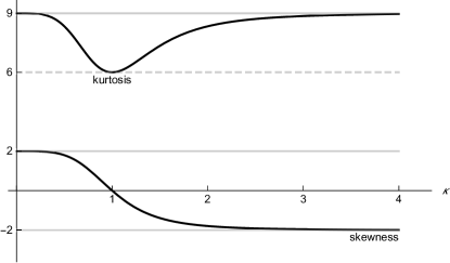
Among them, the mean in (2) is the only one depending on all the parameters of the AL distribution. The mean is given by the mode plus a term whose sign depends on the asymmetry parameter κ𝜅\kappa; this term can be negative (for κ>1𝜅1\kappa>1), null (for κ=1𝜅1\kappa=1), or positive (for κ<1𝜅1\kappa<1). The variance does not depend on the mode μ𝜇\mu and it is given by β2superscript𝛽2\beta^{2} – which is half of the variance 2β22superscript𝛽22\beta^{2} of (μ,β)𝜇𝛽\mathcal{L}\left(\mu,\beta\right) – multiplied by a positive factor only depending on κ𝜅\kappa. Instead, skewness and kurtosis only depend on κ𝜅\kappa, and their behavior as a function of κ𝜅\kappa is displayed in Figure 1.

Refer to caption
Figure 1: Skewness and kurtosis of 𝒜(0,1,κ)𝒜01𝜅\mathcal{AL}\left(0,1,\kappa\right) as a function of κ𝜅\kappa. Grey solid lines represent asymptotes.

The skewness lies in the interval (2,2)22\left(-2,2\right); as κ𝜅\kappa increases, the corresponding value of Skew(X)Skew𝑋\text{Skew}\left(X\right) decreases monotonically. As for the kurtosis, the AL distribution is leptokurtic and Kurt(X)Kurt𝑋\text{Kurt}\left(X\right) varies from 6 – the value we have for the symmetric Laplace distribution (κ=1𝜅1\kappa=1) – to 9 (the greatest value attained when either κ0𝜅0\kappa\rightarrow 0 or κ𝜅\kappa\rightarrow\infty). For further details about moments and related quantities of 𝒜(μ,β,κ)𝒜𝜇𝛽𝜅\mathcal{AL}\left(\mu,\beta,\kappa\right), see Kotz et al. (2012, Section 3.1.5).

2.2 Probability density function

In Definition 1 we introduce the asymmetric Laplace scale mixture in terms of its pdf.

Definition 1 (Probability density function).

A random variable X𝑋X is said to have the asymmetric Laplace scale mixture (ALSM) distribution with location μ(,)𝜇\mu\in\left(-\infty,\infty\right), scale β>0𝛽0\beta>0, asymmetry parameter κ>0𝜅0\kappa>0 and tailedness 𝜽𝜽\bm{\theta}, in symbols X𝒜𝒮(μ,β,κ,𝜽)similar-to𝑋𝒜𝒮𝜇𝛽𝜅𝜽X\sim\mathcal{ALSM}\left(\mu,\beta,\kappa,\bm{\theta}\right), if its pdf is given by

fALSM(x;μ,β,κ,𝜽)=ShfAL(x;μ,β/w,κ)h(w;𝜽)𝑑w,<x<,formulae-sequencesubscript𝑓ALSM𝑥𝜇𝛽𝜅𝜽subscriptsubscript𝑆subscript𝑓AL𝑥𝜇𝛽𝑤𝜅𝑤𝜽differential-d𝑤𝑥f_{\text{ALSM}}\left(x;\mu,\beta,\kappa,\bm{\theta}\right)=\int_{S_{h}}f_{\text{AL}}\left(x;\mu,\beta/w,\kappa\right)h\left(w;\bm{\theta}\right)dw,\quad-\infty<x<\infty, (6)

where h(w;𝜽)𝑤𝜽h\left(w;\bm{\theta}\right) is the mixing probability density (or mass) function of W𝑊W, with support Sh(0,)subscript𝑆0S_{h}\subseteq\left(0,\infty\right), depending on the vector of parameters 𝜽𝜽\bm{\theta}; in symbols, W(𝜽)similar-to𝑊𝜽W\sim\mathcal{H}\left(\bm{\theta}\right).

According to (6), the distribution of X𝑋X can be thought of as a composite distribution constructed by taking a finite/infinite set of AL component distributions with the same location μ𝜇\mu and asymmetry parameter κ𝜅\kappa, but with a different scale β/w𝛽𝑤\beta/w. The component AL distributions are not taken uniformly from the set, but according to a set of “weights” determined by the distribution of W𝑊W (random counterpart of w𝑤w). In the context of modelling currency returns, the mixing variable W𝑊W could be interpreted as a shock that arises from new information and impacts the volatility of the market. The resulting mixture is not itself an AL distribution due to a more flexible tail behavior governed by the tailedness parameter 𝜽𝜽\bm{\theta}. However, the distribution preserves the characteristic towering peak of the AL distribution. Note that, if W𝑊W is degenerate in 1 (W1𝑊1W\equiv 1), then 𝒜𝒮(μ,β,κ,𝜽)𝒜𝒮𝜇𝛽𝜅𝜽\mathcal{ALSM}\left(\mu,\beta,\kappa,\bm{\theta}\right) reduces to 𝒜(μ,β,κ)𝒜𝜇𝛽𝜅\mathcal{AL}\left(\mu,\beta,\kappa\right). While, if κ=1𝜅1\kappa=1, then 𝒜𝒮(μ,β,κ,𝜽)𝒜𝒮𝜇𝛽𝜅𝜽\mathcal{ALSM}\left(\mu,\beta,\kappa,\bm{\theta}\right) reduces to the Laplace scale mixture 𝒮(μ,β,𝜽)𝒮𝜇𝛽𝜽\mathcal{LSM}\left(\mu,\beta,\bm{\theta}\right) distribution proposed by Punzo & Bagnato (2021a).

If we want model (6) to embed 𝒜(μ,β,κ)𝒜𝜇𝛽𝜅\mathcal{AL}\left(\mu,\beta,\kappa\right) as a special or limiting case, we need to consider a mixing random variable W𝑊W degenerating in 1 under a convenient choice of 𝜽𝜽\bm{\theta}. This is commonly required to models that aim to make more flexible the behavior of the tails of a conditional distribution (as, e.g., the well-known normal scale mixture model). This allows to use inferential procedures such as the likelihood-ratio test to compare the ALSM with the nested AL distribution (cf. Section 5).

2.3 Representations

The ALSM admits the following useful representations as mixture of normal distributions (Proposition 1) and as mixture of AL distributions (Proposition 2).

Proposition 1 (Mixture of normal distributions).

X𝒜𝒮(μ,β,κ,𝜽)similar-to𝑋𝒜𝒮𝜇𝛽𝜅𝜽X\sim\mathcal{ALSM}\left(\mu,\beta,\kappa,\bm{\theta}\right) admits the representation

X=dμ+β(1κκ)VW+β2VWZ,superscript𝑑𝑋𝜇𝛽1𝜅𝜅𝑉𝑊𝛽2𝑉𝑊𝑍X\stackrel{{\scriptstyle d}}{{=}}\mu+\beta\left(\frac{1}{\kappa}-\kappa\right)\frac{V}{W}+\beta\frac{\sqrt{2V}}{W}Z, (7)

where Z𝑍Z is standard normal (Z𝒩(0,1)similar-to𝑍𝒩01Z\sim\mathcal{N}\left(0,1\right)) and V𝑉V is standard exponential (V(1)similar-to𝑉1V\sim\mathcal{E}\left(1\right)). Note that Z𝑍Z, V𝑉V, and W𝑊W are independent.

Proposition 2 (Mixture of AL distributions).

X𝒜𝒮(μ,β,κ,𝜽)similar-to𝑋𝒜𝒮𝜇𝛽𝜅𝜽X\sim\mathcal{ALSM}\left(\mu,\beta,\kappa,\bm{\theta}\right) admits the representation

X=dμ+βYW,superscript𝑑𝑋𝜇𝛽𝑌𝑊X\stackrel{{\scriptstyle d}}{{=}}\mu+\beta\frac{Y}{W}, (8)

where Y𝒜(0,1,κ)similar-to𝑌𝒜01𝜅Y\sim\mathcal{AL}\left(0,1,\kappa\right) is independent of W𝑊W.

2.4 Moments

Let X𝒜𝒮(μ,β,κ,𝜽)similar-to𝑋𝒜𝒮𝜇𝛽𝜅𝜽X\sim\mathcal{ALSM}\left(\mu,\beta,\kappa,\bm{\theta}\right). For any integer r>0𝑟0r>0, it can be proved – starting from the representation given in Proposition 2, from Eq. (3.1.25) in Kotz et al. (2001), and noticing that Y𝑌Y and W𝑊W are stochastically independent – that the r𝑟rth moment of X𝑋X about μ𝜇\mu is

E[(Xμ)r]Edelimited-[]superscript𝑋𝜇𝑟\displaystyle\text{E}\left[\left(X-\mu\right)^{r}\right] =E[(Yμ)r]βrE(1Wr)absentEdelimited-[]superscript𝑌𝜇𝑟superscript𝛽𝑟E1superscript𝑊𝑟\displaystyle=\text{E}\left[\left(Y-\mu\right)^{r}\right]\beta^{r}\text{E}\left(\frac{1}{W^{r}}\right)
=r!(βκ)rpr(κ)E(1Wr),absent𝑟superscript𝛽𝜅𝑟subscript𝑝𝑟𝜅E1superscript𝑊𝑟\displaystyle=r!\left(\frac{\beta}{\kappa}\right)^{r}p_{r}\left(\kappa\right)\text{E}\left(\frac{1}{W^{r}}\right), (9)

where

pr(κ)subscript𝑝𝑟𝜅\displaystyle p_{r}\left(\kappa\right) =j=0r(1)jκ2jabsentsuperscriptsubscript𝑗0𝑟superscript1𝑗superscript𝜅2𝑗\displaystyle=\sum_{j=0}^{r}\left(-1\right)^{j}\kappa^{2j}
=1+(1)rκ2(r+1)1+κ2.absent1superscript1𝑟superscript𝜅2𝑟11superscript𝜅2\displaystyle=\frac{\displaystyle 1+\left(-1\right)^{r}\kappa^{2(r+1)}}{1+\kappa^{2}}. (10)

The moment in (9) exists if E(1/Wr)<E1superscript𝑊𝑟\text{E}\left(1/W^{r}\right)<\infty.

2.5 Absolute moments

Let X𝒜𝒮(μ,β,κ,𝜽)similar-to𝑋𝒜𝒮𝜇𝛽𝜅𝜽X\sim\mathcal{ALSM}\left(\mu,\beta,\kappa,\bm{\theta}\right). For any a>1𝑎1a>-1, it can be proved – starting from the representation given in Proposition 1, from Eq. (3.1.26) in Kotz et al. (2001), and noticing that Y𝑌Y and W𝑊W are stochastically independent – that the absolute moment of order a𝑎a of X𝑋X about μ𝜇\mu is

E[|Xμ|a]Edelimited-[]superscript𝑋𝜇𝑎\displaystyle\text{E}\left[\left|X-\mu\right|^{a}\right] =E[|Yμ|a]βaE(1Wa)absentEdelimited-[]superscript𝑌𝜇𝑎superscript𝛽𝑎𝐸1superscript𝑊𝑎\displaystyle=\text{E}\left[\left|Y-\mu\right|^{a}\right]\beta^{a}E\left(\frac{1}{W^{a}}\right)
=(βκ)aΓ(a+1)1+κ2(a+1)1+κ2E(1Wa).absentsuperscript𝛽𝜅𝑎Γ𝑎11superscript𝜅2𝑎11superscript𝜅2E1superscript𝑊𝑎\displaystyle=\left(\frac{\beta}{\kappa}\right)^{a}\Gamma\left(a+1\right)\frac{\displaystyle 1+\kappa^{2(a+1)}}{1+\kappa^{2}}\text{E}\left(\frac{1}{W^{a}}\right). (11)

The moment in (11) exists if E(1/Wa)<E1superscript𝑊𝑎\text{E}\left(1/W^{a}\right)<\infty.

2.6 Mean, variance, skewness, and kurtosis

Mean, variance, skewness, and kurtosis of X𝒜𝒮(μ,β,κ,𝜽)similar-to𝑋𝒜𝒮𝜇𝛽𝜅𝜽X\sim\mathcal{ALSM}\left(\mu,\beta,\kappa,\bm{\theta}\right) can be obtained from (8) and from the corresponding moments of 𝒜(μ,β,κ)𝒜𝜇𝛽𝜅\mathcal{AL}\left(\mu,\beta,\kappa\right). These moments can be expressed as a function of convenient moments of 1/W1𝑊1/W, which depend on 𝜽𝜽\bm{\theta}, in the following way:

E(X)E𝑋\displaystyle\text{E}\left(X\right) =μ+βE(Y)E(1W)absent𝜇𝛽E𝑌E1𝑊\displaystyle=\mu+\beta\text{E}\left(Y\right)\text{E}\left(\frac{1}{W}\right)
=μ+βκp1(κ)E(1W)absent𝜇𝛽𝜅subscript𝑝1𝜅E1𝑊\displaystyle=\mu+\frac{\beta}{\kappa}p_{1}\left(\kappa\right)\text{E}\left(\frac{1}{W}\right)
=μ+β(1κκ)E(1W)absent𝜇𝛽1𝜅𝜅E1𝑊\displaystyle=\mu+\beta\left(\frac{1}{\kappa}-\kappa\right)\text{E}\left(\frac{1}{W}\right) (12)
Var(X)Var𝑋\displaystyle\text{Var}\left(X\right) =β2Var(YW)absentsuperscript𝛽2Var𝑌𝑊\displaystyle=\beta^{2}\text{Var}\left(\frac{Y}{W}\right)
=β2κ2[2p2(κ)E(1W2)p1(κ)2E(1W)2],absentsuperscript𝛽2superscript𝜅2delimited-[]2subscript𝑝2𝜅E1superscript𝑊2subscript𝑝1superscript𝜅2Esuperscript1𝑊2\displaystyle=\frac{\beta^{2}}{\kappa^{2}}\left[2p_{2}(\kappa)\text{E}\left(\frac{1}{W^{2}}\right)-p_{1}(\kappa)^{2}\text{E}\left(\frac{1}{W}\right)^{2}\right],
=β2κ2(1+κ2)[2(1+κ6)E(1W2)(1κ4)(1κ2)E(1W)2]absentsuperscript𝛽2superscript𝜅21superscript𝜅2delimited-[]21superscript𝜅6E1superscript𝑊21superscript𝜅41superscript𝜅2Esuperscript1𝑊2\displaystyle=\frac{\beta^{2}}{\kappa^{2}\left(1+\kappa^{2}\right)}\left[2\left(1+\kappa^{6}\right)\text{E}\left(\frac{1}{W^{2}}\right)-\left(1-\kappa^{4}\right)\left(1-\kappa^{2}\right)\text{E}\left(\frac{1}{W}\right)^{2}\right] (13)
Skew(X)Skew𝑋\displaystyle\text{Skew}\left(X\right) =23p3(κ)E(1W3)3p2(κ)p1(κ)E(1W2)E(1W)+p1(κ)3E(1W)3[2p2(κ)E(1W2)p1(κ)2E(1W)2]32,absent23subscript𝑝3𝜅E1superscript𝑊33subscript𝑝2𝜅subscript𝑝1𝜅E1superscript𝑊2E1𝑊subscript𝑝1superscript𝜅3Esuperscript1𝑊3superscriptdelimited-[]2subscript𝑝2𝜅E1superscript𝑊2subscript𝑝1superscript𝜅2Esuperscript1𝑊232\displaystyle=2\frac{3p_{3}(\kappa)\text{E}\left(\frac{1}{W^{3}}\right)-3p_{2}(\kappa)p_{1}(\kappa)\text{E}\left(\frac{1}{W^{2}}\right)\text{E}\left(\frac{1}{W}\right)+p_{1}(\kappa)^{3}\text{E}\left(\frac{1}{W}\right)^{3}}{\left[2p_{2}(\kappa)\text{E}\left(\frac{1}{W^{2}}\right)-p_{1}(\kappa)^{2}\text{E}\left(\frac{1}{W}\right)^{2}\right]^{\frac{3}{2}}},
=23(1+κ2)2(1κ8)E(1W3)3(1+κ2)(1+κ6)(1κ4)E(1W2)E(1W)+(1κ8)3E(1W)3[2(1+κ2)(1+κ6)E(1W2)(1κ4)2E(1W)2]32,absent23superscript1superscript𝜅221superscript𝜅8E1superscript𝑊331superscript𝜅21superscript𝜅61superscript𝜅4E1superscript𝑊2E1𝑊superscript1superscript𝜅83Esuperscript1𝑊3superscriptdelimited-[]21superscript𝜅21superscript𝜅6E1superscript𝑊2superscript1superscript𝜅42Esuperscript1𝑊232\displaystyle=2\frac{3\left(1+\kappa^{2}\right)^{2}\left(1-\kappa^{8}\right)\text{E}\left(\frac{1}{W^{3}}\right)-3\left(1+\kappa^{2}\right)\left(1+\kappa^{6}\right)\left(1-\kappa^{4}\right)\text{E}\left(\frac{1}{W^{2}}\right)\text{E}\left(\frac{1}{W}\right)+\left(1-\kappa^{8}\right)^{3}\text{E}\left(\frac{1}{W}\right)^{3}}{\left[2\left(1+\kappa^{2}\right)\left(1+\kappa^{6}\right)\text{E}\left(\frac{1}{W^{2}}\right)-\left(1-\kappa^{4}\right)^{2}\text{E}\left(\frac{1}{W}\right)^{2}\right]^{\frac{3}{2}}}, (14)
Kurt(X)Kurt𝑋\displaystyle\text{Kurt}\left(X\right) =122p4(κ)E(1W4)2p3(κ)p1(κ)E(1W3)E(1W)+p2(κ)2E(1W2)2[2p2(κ)E(1W2)p1(κ)2E(1W)2]23absent122subscript𝑝4𝜅E1superscript𝑊42subscript𝑝3𝜅subscript𝑝1𝜅E1superscript𝑊3E1𝑊subscript𝑝2superscript𝜅2Esuperscript1superscript𝑊22superscriptdelimited-[]2subscript𝑝2𝜅E1superscript𝑊2subscript𝑝1superscript𝜅2Esuperscript1𝑊223\displaystyle=12\frac{2p_{4}(\kappa)\text{E}\left(\frac{1}{W^{4}}\right)-2p_{3}(\kappa)p_{1}(\kappa)\text{E}\left(\frac{1}{W^{3}}\right)\text{E}\left(\frac{1}{W}\right)+p_{2}(\kappa)^{2}\text{E}\left(\frac{1}{W^{2}}\right)^{2}}{\left[2p_{2}(\kappa)\text{E}\left(\frac{1}{W^{2}}\right)-p_{1}(\kappa)^{2}\text{E}\left(\frac{1}{W}\right)^{2}\right]^{2}}-3
=122(1+κ2)(1+κ10)E(1W4)2(1κ8)(1κ4)E(1W3)E(1W)+(1+κ6)2E(1W2)2[2(1+κ6)E(1W2)(1κ2)(1κ4)E(1W)2]23.absent1221superscript𝜅21superscript𝜅10E1superscript𝑊421superscript𝜅81superscript𝜅4E1superscript𝑊3E1𝑊superscript1superscript𝜅62Esuperscript1superscript𝑊22superscriptdelimited-[]21superscript𝜅6E1superscript𝑊21superscript𝜅21superscript𝜅4Esuperscript1𝑊223\displaystyle=12\frac{2\left(1+\kappa^{2}\right)\left(1+\kappa^{10}\right)\text{E}\left(\frac{1}{W^{4}}\right)-2\left(1-\kappa^{8}\right)\left(1-\kappa^{4}\right)\text{E}\left(\frac{1}{W^{3}}\right)\text{E}\left(\frac{1}{W}\right)+\left(1+\kappa^{6}\right)^{2}\text{E}\left(\frac{1}{W^{2}}\right)^{2}}{\left[2\left(1+\kappa^{6}\right)\text{E}\left(\frac{1}{W^{2}}\right)-\left(1-\kappa^{2}\right)\left(1-\kappa^{4}\right)\text{E}\left(\frac{1}{W}\right)^{2}\right]^{2}}-3. (15)

As we can note, the mean depends on all the parameters of the ALSM distribution, the variance does not depend on μ𝜇\mu, while skewness and kurtosis only depend on κ𝜅\kappa and 𝜽𝜽\bm{\theta}.

2.7 Mode

In Theorem 1 we show that the ALSM distribution is unimodal hump-shaped, with mode in μ𝜇\mu; the result is a slight modification of Theorem 1 in Punzo et al. (2018) and Punzo & Bagnato (2021a).

Theorem 1.

The pdf of X𝒜𝒮(μ,β,κ,𝜽)similar-to𝑋𝒜𝒮𝜇𝛽𝜅𝜽X\sim\mathcal{ALSM}\left(\mu,\beta,\kappa,\bm{\theta}\right) is unimodal hump-shaped in x=μ𝑥𝜇x=\mu.

Proof. The first derivative, with respect to x𝑥x, of fALSM(x;μ,β,κ,𝜽)subscript𝑓ALSM𝑥𝜇𝛽𝜅𝜽f_{\text{ALSM}}\left(x;\mu,\beta,\kappa,\bm{\theta}\right) is

fALSM(x;μ,β,κ,𝜽)=ShfAL(x;μ,β/w,κ)h(w;𝜽)𝑑w,x>0,formulae-sequencesuperscriptsubscript𝑓ALSM𝑥𝜇𝛽𝜅𝜽subscriptsubscript𝑆superscriptsubscript𝑓AL𝑥𝜇𝛽𝑤𝜅𝑤𝜽differential-d𝑤𝑥0f_{\text{ALSM}}^{\prime}\left(x;\mu,\beta,\kappa,\bm{\theta}\right)=\int_{S_{h}}f_{\text{AL}}^{\prime}\left(x;\mu,\beta/w,\kappa\right)h\left(w;\bm{\theta}\right)dw,\quad x>0,

where

fAL(x;μ,β/w,κ)=w2β2κ21+κ2(μx){ewκβ(xμ)for xμ,ewκβ(μx)for x<μ.superscriptsubscript𝑓AL𝑥𝜇𝛽𝑤𝜅superscript𝑤2superscript𝛽2superscript𝜅21superscript𝜅2𝜇𝑥casessuperscript𝑒𝑤𝜅𝛽𝑥𝜇for xμsuperscript𝑒𝑤𝜅𝛽𝜇𝑥for x<μf_{\text{AL}}^{\prime}\left(x;\mu,\beta/w,\kappa\right)=\frac{w^{2}}{\beta^{2}}\frac{\kappa^{2}}{1+\kappa^{2}}(\mu-x)\begin{cases}e^{-\frac{w\kappa}{\beta}\left(x-\mu\right)}&\text{for $x\geq\mu$},\\ e^{-\frac{w}{\kappa\beta}\left(\mu-x\right)}&\text{for $x<\mu$}.\end{cases}

Hence, fAL(x;μ,β/w,κ)>0superscriptsubscript𝑓AL𝑥𝜇𝛽𝑤𝜅0f_{\text{AL}}^{\prime}\left(x;\mu,\beta/w,\kappa\right)>0 for x<μ𝑥𝜇x<\mu, fAL(x;μ,β/w,κ)<0superscriptsubscript𝑓AL𝑥𝜇𝛽𝑤𝜅0f_{\text{AL}}^{\prime}\left(x;\mu,\beta/w,\kappa\right)<0 for x>μ𝑥𝜇x>\mu, and fAL(x;μ,β/w,κ)=0superscriptsubscript𝑓AL𝑥𝜇𝛽𝑤𝜅0f_{\text{AL}}^{\prime}\left(x;\mu,\beta/w,\kappa\right)=0 for x=μ𝑥𝜇x=\mu. Using these results and recalling that h(w;𝜽)>0𝑤𝜽0h\left(w;\bm{\theta}\right)>0 for w>0𝑤0w>0, the theorem is straightforwardly proven. ∎

3 Examples of asymmetric Laplace scale mixtures

The ALSM family of distributions is extremely flexible. In this section we introduce some members of the family obtained under a convenient choice of the mixing probability density (or mass) function h(w;𝜽)𝑤𝜽h\left(w;\bm{\theta}\right). These members satisfy two requirements: 1) the existence of a closed-form pdf for the ALSM and 2) the peculiarity to nest 𝒜(μ,β,κ)𝒜𝜇𝛽𝜅\mathcal{AL}\left(\mu,\beta,\kappa\right) under a suitable choice of 𝜽𝜽\bm{\theta}.

3.1 Two-point asymmetric Laplace distribution

A simple but effective special case of model (6) is obtained if we consider the following mixing two-point (TP) distribution

W={1with probability θ11/θ2with probability 1θ1,𝑊cases1with probability θ11subscript𝜃2with probability 1θ1W=\begin{cases}1&\text{with probability $\theta_{1}$}\\ 1/\theta_{2}&\text{with probability $1-\theta_{1}$},\\ \end{cases} (16)

where θ1(0,1)subscript𝜃101\theta_{1}\in\left(0,1\right) and θ2>1subscript𝜃21\theta_{2}>1. The probability mass function of W𝑊W is

h(w;𝜽)=θ1w1/θ211/θ2(1θ1)1w11/θ2,w{1/θ2,1},formulae-sequence𝑤𝜽superscriptsubscript𝜃1𝑤1subscript𝜃211subscript𝜃2superscript1subscript𝜃11𝑤11subscript𝜃2𝑤1subscript𝜃21h\left(w;\bm{\theta}\right)=\theta_{1}^{\frac{w-1/\theta_{2}}{1-1/\theta_{2}}}\left(1-\theta_{1}\right)^{\frac{1-w}{1-1/\theta_{2}}},\quad w\in\left\{1/\theta_{2},1\right\}, (17)

where 𝜽=(θ1,θ2)𝜽superscriptsubscript𝜃1subscript𝜃2\bm{\theta}=\left(\theta_{1},\theta_{2}\right)^{\prime}; in symbols, W𝒯𝒫{1/θ2,1}(θ1)similar-to𝑊𝒯subscript𝒫1subscript𝜃21subscript𝜃1W\sim\mathcal{TP}_{\left\{1/\theta_{2},1\right\}}\left(\theta_{1}\right). Using (17), model (6) becomes

fALSM(x;μ,β,κ,𝜽)=θ1fAL(x;μ,β,κ)+(1θ1)fAL(x;μ,θ2β,κ),<x<.formulae-sequencesubscript𝑓ALSM𝑥𝜇𝛽𝜅𝜽subscript𝜃1subscript𝑓AL𝑥𝜇𝛽𝜅1subscript𝜃1subscript𝑓AL𝑥𝜇subscript𝜃2𝛽𝜅𝑥f_{\text{ALSM}}\left(x;\mu,\beta,\kappa,\bm{\theta}\right)=\theta_{1}f_{\text{AL}}\left(x;\mu,\beta,\kappa\right)+\left(1-\theta_{1}\right)f_{\text{AL}}\left(x;\mu,\theta_{2}\beta,\kappa\right),\quad-\infty<x<\infty. (18)

Hereafter, we will refer to the resulting distribution as two-point asymmetric Laplace (TP-AL).

If W𝒯𝒫{1/θ2,1}(θ1)similar-to𝑊𝒯subscript𝒫1subscript𝜃21subscript𝜃1W\sim\mathcal{TP}_{\left\{1/\theta_{2},1\right\}}\left(\theta_{1}\right), then the r𝑟rth moment of 1/W1𝑊1/W is

E(1Wr)=θ1+(1θ1)θ2r.E1superscript𝑊𝑟subscript𝜃11subscript𝜃1superscriptsubscript𝜃2𝑟\text{E}\left(\frac{1}{W^{r}}\right)=\theta_{1}+\left(1-\theta_{1}\right)\theta_{2}^{r}. (19)

If we put in (11)–(15) the first four raw moments computed according to (19), mean, variance, skewness and kurtosis of the TP-AL distribution become

E(X)=μ+β(1κκ)[θ1+(1θ1)θ2],E𝑋𝜇𝛽1𝜅𝜅delimited-[]subscript𝜃11subscript𝜃1subscript𝜃2\text{E}\left(X\right)=\mu+\beta\left(\frac{1}{\kappa}-\kappa\right)\left[\theta_{1}+\left(1-\theta_{1}\right)\theta_{2}\right], (20)
Var(X)=β2κ2{2[θ1+(1θ1)θ2](1+κ6)1+κ2[θ1+(1θ1)θ2]2(1κ4)2(1+κ2)2},Var𝑋superscript𝛽2superscript𝜅22delimited-[]subscript𝜃11subscript𝜃1subscript𝜃21superscript𝜅61superscript𝜅2superscriptdelimited-[]subscript𝜃11subscript𝜃1subscript𝜃22superscript1superscript𝜅42superscript1superscript𝜅22\text{Var}\left(X\right)=\frac{\beta^{2}}{\kappa^{2}}\left\{\frac{2\left[\theta_{1}+\left(1-\theta_{1}\right)\theta_{2}\right]\left(1+\kappa^{6}\right)}{1+\kappa^{2}}-\frac{\left[\theta_{1}+\left(1-\theta_{1}\right)\theta_{2}\right]^{2}\left(1-\kappa^{4}\right)^{2}}{\left(1+\kappa^{2}\right)^{2}}\right\}, (21)
Skew(X)=2{[θ1+(1θ1)θ2]2(1κ4)33[θ1+(1θ1)θ2](1+κ2)(1+κ6)(1κ4)+3(1+κ2)2(1κ8)}θ1+(1θ1)θ2{2(1+κ2)(1+κ6)[θ1+(1θ1)θ2](1κ4)2}3/2,Skew𝑋2superscriptdelimited-[]subscript𝜃11subscript𝜃1subscript𝜃22superscript1superscript𝜅433delimited-[]subscript𝜃11subscript𝜃1subscript𝜃21superscript𝜅21superscript𝜅61superscript𝜅43superscript1superscript𝜅221superscript𝜅8subscript𝜃11subscript𝜃1subscript𝜃2superscript21superscript𝜅21superscript𝜅6delimited-[]subscript𝜃11subscript𝜃1subscript𝜃2superscript1superscript𝜅4232\text{Skew}\left(X\right)=\frac{2\left\{\left[\theta_{1}+\left(1-\theta_{1}\right)\theta_{2}\right]^{2}\left(1-\kappa^{4}\right)^{3}-3\left[\theta_{1}+\left(1-\theta_{1}\right)\theta_{2}\right]\left(1+\kappa^{2}\right)\left(1+\kappa^{6}\right)\left(1-\kappa^{4}\right)+3\left(1+\kappa^{2}\right)^{2}\left(1-\kappa^{8}\right)\right\}}{\sqrt{\theta_{1}+\left(1-\theta_{1}\right)\theta_{2}}\left\{2\left(1+\kappa^{2}\right)\left(1+\kappa^{6}\right)-\left[\theta_{1}+\left(1-\theta_{1}\right)\theta_{2}\right]\left(1-\kappa^{4}\right)^{2}\right\}^{3/2}}, (22)

and

Kurt(X)=12(1+κ2)2{[θ1+(1θ1)θ2]2(1+κ6)22[θ1+(1θ1)θ2](1κ4)(1κ8)+2(1+κ2)(1+κ10)}[θ1+(1θ1)θ2]{2(1+κ2)(1+κ6)[θ1+(1θ1)θ2](1κ4)2}23.Kurt𝑋12superscript1superscript𝜅22superscriptdelimited-[]subscript𝜃11subscript𝜃1subscript𝜃22superscript1superscript𝜅622delimited-[]subscript𝜃11subscript𝜃1subscript𝜃21superscript𝜅41superscript𝜅821superscript𝜅21superscript𝜅10delimited-[]subscript𝜃11subscript𝜃1subscript𝜃2superscript21superscript𝜅21superscript𝜅6delimited-[]subscript𝜃11subscript𝜃1subscript𝜃2superscript1superscript𝜅4223\text{Kurt}\left(X\right)=\frac{12\left(1+\kappa^{2}\right)^{2}\left\{\left[\theta_{1}+\left(1-\theta_{1}\right)\theta_{2}\right]^{2}\left(1+\kappa^{6}\right)^{2}-2\left[\theta_{1}+\left(1-\theta_{1}\right)\theta_{2}\right]\left(1-\kappa^{4}\right)\left(1-\kappa^{8}\right)+2\left(1+\kappa^{2}\right)\left(1+\kappa^{10}\right)\right\}}{\left[\theta_{1}+\left(1-\theta_{1}\right)\theta_{2}\right]\left\{2\left(1+\kappa^{2}\right)\left(1+\kappa^{6}\right)-\left[\theta_{1}+\left(1-\theta_{1}\right)\theta_{2}\right]\left(1-\kappa^{4}\right)^{2}\right\}^{2}}-3. (23)

With respect to 𝒜(μ,β,κ)𝒜𝜇𝛽𝜅\mathcal{AL}\left(\mu,\beta,\kappa\right), which can be considered as the reference distribution for the model (for a discussion about the concept of reference distribution, see Davies & Gather, 1993), the additional parameters θ1subscript𝜃1\theta_{1} and θ2subscript𝜃2\theta_{2} have an interpretation of practical interest.

θ1subscript𝜃1\theta_{1} is the proportion of points from the reference distribution. For applications of model (18) in robustness studies, it could be natural to assume, and we will do that hereafter, that θ1(1/2,1)subscript𝜃1121\theta_{1}\in\left(1/2,1\right), i.e., at least half of the observations come from the reference distribution (Hennig, 2002, p. 250, Punzo & McNicholas, 2016, Mazza & Punzo, 2019, Templ et al., 2019 and Punzo & Bagnato, 2021a).

θ2subscript𝜃2\theta_{2} denotes the degree of contamination and, because of the assumption θ2>1subscript𝜃21\theta_{2}>1, it can be meant as the increase in variability due to the points which do not come from the reference distribution; hence, it is an inflation parameter.

Model (18) reduces to 𝒜(μ,β,κ)𝒜𝜇𝛽𝜅\mathcal{AL}\left(\mu,\beta,\kappa\right) when θ11subscript𝜃11\theta_{1}\rightarrow 1 and θ21subscript𝜃21\theta_{2}\rightarrow 1, and can also be seen as the natural asymmetric counterpart of the contaminated Laplace distribution introduced by Punzo & Bagnato (2021a). For this reason, we will also refer to the TP-AL distribution as contaminated asymmetric Laplace distribution.

An interesting characteristic of model (18) is the possibility to determine whether a generic observation x𝑥x comes or not from the reference distribution via the a posteriori probability

P(x comes from 𝒜(μ,β,κ)|μ,β,κ,𝜽)=θ1fAL(x;μ,β,κ)fALSM(x;μ,β,κ,𝜽).𝑃conditionalx comes from 𝒜(μ,β,κ)𝜇𝛽𝜅𝜽subscript𝜃1subscript𝑓AL𝑥𝜇𝛽𝜅subscript𝑓ALSM𝑥𝜇𝛽𝜅𝜽P\left(\text{$x$ comes from $\mathcal{AL}\left(\mu,\beta,\kappa\right)$}\left|\mu,\beta,\kappa,\bm{\theta}\right.\right)=\frac{\theta_{1}f_{\text{AL}}\left(x;\mu,\beta,\kappa\right)}{f_{\text{ALSM}}\left(x;\mu,\beta,\kappa,\bm{\theta}\right)}. (24)

Specifically, x𝑥x will be considered coming from the reference distribution if the probability in (24) is greater than 1/2.

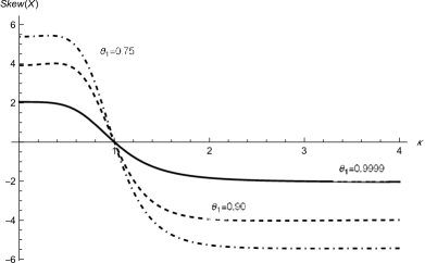
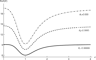
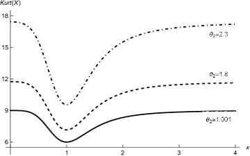
Figure 2 shows examples of behaviors of Skew(X)Skew𝑋\text{Skew}\left(X\right) and Kurt(X)Kurt𝑋\text{Kurt}\left(X\right), as functions of κ𝜅\kappa, at various levels of θ1subscript𝜃1\theta_{1}, with θ2=5subscript𝜃25\theta_{2}=5.

Refer to caption
(a) Skewness
Refer to caption
(b) Kurtosis
Figure 2: Examples of behavior of Skew(X)Skew𝑋\text{Skew}\left(X\right) (on the left) and Kurt(X)Kurt𝑋\text{Kurt}\left(X\right) (on the right), as functions of κ𝜅\kappa, at various levels of θ1subscript𝜃1\theta_{1} for the TP-AL distribution, with θ2=5subscript𝜃25\theta_{2}=5.

From Figure 2(a) we realize that: 1) values of θ1subscript𝜃1\theta_{1} close to 1 tend to produce the plot of Skew(X)Skew𝑋\text{Skew}\left(X\right) we obtained for 𝒜(μ,β,κ)𝒜𝜇𝛽𝜅\mathcal{AL}\left(\mu,\beta,\kappa\right) (refer to Figure 1); and 2) as θ1subscript𝜃1\theta_{1} decreases (to a minimum value of 0.5), the range of possible values of Skew(X)Skew𝑋\text{Skew}\left(X\right) increases. Similarly, from Figure 2(b) we realize that, fixed θ2subscript𝜃2\theta_{2}: 1) large values of θ2subscript𝜃2\theta_{2} (with a maximum of 1) tend to produce the plot of Kurt(X)Kurt𝑋\text{Kurt}\left(X\right) we obtained for 𝒜(μ,β,κ)𝒜𝜇𝛽𝜅\mathcal{AL}\left(\mu,\beta,\kappa\right) (refer to Figure 1); and 2) κ𝜅\kappa kept fixed, the lower the value θ1subscript𝜃1\theta_{1} (with a minimum of 0.5), the higher the kurtosis. This means that the curve obtained for θ11subscript𝜃11\theta_{1}\rightarrow 1 acts as a lower bound.

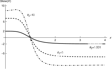
Figure 3 shows examples of behaviors of Skew(X)Skew𝑋\text{Skew}\left(X\right) and Kurt(X)Kurt𝑋\text{Kurt}\left(X\right), as functions of κ𝜅\kappa, at various levels of θ2subscript𝜃2\theta_{2}, with θ1=0.95subscript𝜃10.95\theta_{1}=0.95.

Refer to caption
(a) Skewness
Refer to caption
(b) Kurtosis
Figure 3: Examples of behavior of Skew(X)Skew𝑋\text{Skew}\left(X\right) (on the left) and Kurt(X)Kurt𝑋\text{Kurt}\left(X\right) (on the right), as functions of κ𝜅\kappa, at various levels of θ2subscript𝜃2\theta_{2} for the TP-AL distribution, with θ1=0.95subscript𝜃10.95\theta_{1}=0.95.

From Figure 3(a) we realize that: 1) values of θ2subscript𝜃2\theta_{2} close to 1 tend to produce the plot of Skew(X)Skew𝑋\text{Skew}\left(X\right) we obtained for 𝒜(μ,β,κ)𝒜𝜇𝛽𝜅\mathcal{AL}\left(\mu,\beta,\kappa\right) (refer to Figure 1); and 2) as θ2subscript𝜃2\theta_{2} grows, the range of possible values of Skew(X)Skew𝑋\text{Skew}\left(X\right) increases. Similarly, from Figure 3(b) we realize that: 1) small values of θ𝜃\theta (with a minimum of 1) tend to produce the plot of Kurt(X)Kurt𝑋\text{Kurt}\left(X\right) we obtained for 𝒜(μ,β,κ)𝒜𝜇𝛽𝜅\mathcal{AL}\left(\mu,\beta,\kappa\right) (refer to Figure 1); and 2) κ𝜅\kappa kept fixed, the higher the value θ2subscript𝜃2\theta_{2}, the higher the kurtosis. This means that the curve obtained for θ21subscript𝜃21\theta_{2}\rightarrow 1 acts as a lower bound.

3.2 Shifted exponential Laplace distribution

Let

h(w;θ)=θeθ(w1),w>1,formulae-sequence𝑤𝜃𝜃superscript𝑒𝜃𝑤1𝑤1h\left(w;\theta\right)=\theta e^{-\theta\left(w-1\right)},\quad w>1, (25)

with rate parameter θ>0𝜃0\theta>0, be the pdf of the shifted exponential, in symbols W𝒮(1,)(θ)similar-to𝑊𝒮subscript1𝜃W\sim\mathcal{SE}_{\left(1,\infty\right)}\left(\theta\right). When the pdf in (25) is considered as mixing density in model (6), the pdf of the ALSM becomes

fALSM(x;μ,β,κ,θ)=θβκ1+κ2{1+θ+κβ(xμ)[θ+κβ(xμ)]2eκβ(xμ)for xμ,1+θ+1βκ(μx)[θ+1βκ(μx)]2e1κβ(μx)for x<μ.subscript𝑓ALSM𝑥𝜇𝛽𝜅𝜃𝜃𝛽𝜅1superscript𝜅2cases1𝜃𝜅𝛽𝑥𝜇superscriptdelimited-[]𝜃𝜅𝛽𝑥𝜇2superscript𝑒𝜅𝛽𝑥𝜇for xμ1𝜃1𝛽𝜅𝜇𝑥superscriptdelimited-[]𝜃1𝛽𝜅𝜇𝑥2superscript𝑒1𝜅𝛽𝜇𝑥for x<μf_{\text{ALSM}}\left(x;\mu,\beta,\kappa,\theta\right)=\frac{\theta}{\beta}\frac{\kappa}{1+\kappa^{2}}\begin{cases}\displaystyle\frac{1+\theta+\frac{\kappa}{\beta}\left(x-\mu\right)}{\left[\theta+\frac{\kappa}{\beta}\left(x-\mu\right)\right]^{2}}e^{-\frac{\kappa}{\beta}\left(x-\mu\right)}&\text{for $x\geq\mu$},\\[17.07164pt] \displaystyle\frac{1+\theta+\frac{1}{\beta\kappa}\left(\mu-x\right)}{\left[\theta+\frac{1}{\beta\kappa}\left(\mu-x\right)\right]^{2}}e^{-\frac{1}{\kappa\beta}\left(\mu-x\right)}&\text{for $x<\mu$}.\end{cases} (26)

We will refer to the resulting distribution as shifted exponential asymmetric Laplace (SE-AL). Model (26) reduces to 𝒜(μ,β,κ)𝒜𝜇𝛽𝜅\mathcal{AL}\left(\mu,\beta,\kappa\right) when θ𝜃\theta\rightarrow\infty. Moreover, if κ=1𝜅1\kappa=1, then we obtain the SE-Laplace distribution, proposed by Punzo & Bagnato (2021a), as a special case.

If W𝒮(1,)(θ)similar-to𝑊𝒮subscript1𝜃W\sim\mathcal{SE}_{\left(1,\infty\right)}\left(\theta\right), then the r𝑟rth raw moment of 1/W1𝑊1/W is

E(1Wr)=θeθEr(θ),E1superscript𝑊𝑟𝜃superscript𝑒𝜃subscript𝐸𝑟𝜃\text{E}\left(\frac{1}{W^{r}}\right)=\theta e^{\theta}E_{r}(\theta), (27)

where En(z)=1ezt/tn𝑑tsubscript𝐸𝑛𝑧superscriptsubscript1superscript𝑒𝑧𝑡superscript𝑡𝑛differential-d𝑡E_{n}\left(z\right)=\int_{1}^{\infty}e^{-zt}/t^{n}dt is the exponential integral function. By substituting in (12)–(15) the first four raw moments computed according to (27), mean, variance, skewness and kurtosis of the SE-AL distribution become

E(X)=μ+β(1κκ)θeθE1(θ),E𝑋𝜇𝛽1𝜅𝜅𝜃superscript𝑒𝜃subscript𝐸1𝜃\text{E}\left(X\right)=\mu+\beta\left(\frac{1}{\kappa}-\kappa\right)\theta e^{\theta}E_{1}(\theta), (28)
Var(X)=β2θeθκ2(1+κ2)[2(1+κ6)E2(θ)θeθ(1κ4)(1κ2)E1(θ)2],Var𝑋superscript𝛽2𝜃superscript𝑒𝜃superscript𝜅21superscript𝜅2delimited-[]21superscript𝜅6subscript𝐸2𝜃𝜃superscript𝑒𝜃1superscript𝜅41superscript𝜅2subscript𝐸1superscript𝜃2\text{Var}\left(X\right)=\frac{\beta^{2}\theta e^{\theta}}{\kappa^{2}\left(1+\kappa^{2}\right)}\left[2\left(1+\kappa^{6}\right)E_{2}(\theta)-\theta e^{\theta}\left(1-\kappa^{4}\right)\left(1-\kappa^{2}\right)E_{1}(\theta)^{2}\right], (29)
Skew(X)=3(1+κ2)2(1κ8)E3(θ)3θeθ(1+κ2)(1+κ6)(1κ4)E2(θ)E1(θ)+(1κ8)3θ2e2θE1(θ)3θeθ[2(1+κ2)(1+κ6)E2(θ)θeθ(1κ4)2E1(θ)2]32,Skew𝑋3superscript1superscript𝜅221superscript𝜅8subscript𝐸3𝜃3𝜃superscript𝑒𝜃1superscript𝜅21superscript𝜅61superscript𝜅4subscript𝐸2𝜃subscript𝐸1𝜃superscript1superscript𝜅83superscript𝜃2superscript𝑒2𝜃subscript𝐸1superscript𝜃3𝜃superscript𝑒𝜃superscriptdelimited-[]21superscript𝜅21superscript𝜅6subscript𝐸2𝜃𝜃superscript𝑒𝜃superscript1superscript𝜅42subscript𝐸1superscript𝜃232\text{Skew}\left(X\right)=\frac{3\left(1+\kappa^{2}\right)^{2}\left(1-\kappa^{8}\right)E_{3}(\theta)-3\theta e^{\theta}\left(1+\kappa^{2}\right)\left(1+\kappa^{6}\right)\left(1-\kappa^{4}\right)E_{2}(\theta)E_{1}(\theta)+\left(1-\kappa^{8}\right)^{3}\theta^{2}e^{2\theta}E_{1}(\theta)^{3}}{\sqrt{\theta e^{\theta}}\left[2\left(1+\kappa^{2}\right)\left(1+\kappa^{6}\right)E_{2}(\theta)-\theta e^{\theta}\left(1-\kappa^{4}\right)^{2}E_{1}(\theta)^{2}\right]^{\frac{3}{2}}}, (30)

and

Kurt(X)=12θeθ2(1+κ2)(1+κ10)E4(θ)2θeθ(1κ8)(1κ4)E1(θ)E3(θ)eθθ(1+κ6)2E2(θ)2[eθθ(1κ2)(1κ4)E1(θ)22(1+κ6)E2(θ)]23Kurt𝑋12𝜃superscript𝑒𝜃21superscript𝜅21superscript𝜅10subscript𝐸4𝜃2𝜃superscript𝑒𝜃1superscript𝜅81superscript𝜅4subscript𝐸1𝜃subscript𝐸3𝜃superscript𝑒𝜃𝜃superscript1superscript𝜅62subscript𝐸2superscript𝜃2superscriptdelimited-[]superscript𝑒𝜃𝜃1superscript𝜅21superscript𝜅4subscript𝐸1superscript𝜃221superscript𝜅6subscript𝐸2𝜃23\text{Kurt}\left(X\right)=\frac{12}{\theta e^{\theta}}\cdot\frac{2\left(1+\kappa^{2}\right)\left(1+\kappa^{10}\right)E_{4}(\theta)-2\theta e^{\theta}\left(1-\kappa^{8}\right)\left(1-\kappa^{4}\right)E_{1}(\theta)E_{3}(\theta)e^{\theta}\theta\left(1+\kappa^{6}\right)^{2}E_{2}(\theta)^{2}}{\left[e^{\theta}\theta\left(1-\kappa^{2}\right)\left(1-\kappa^{4}\right)E_{1}(\theta)^{2}-2\left(1+\kappa^{6}\right)E_{2}(\theta)\right]^{2}}-3 (31)

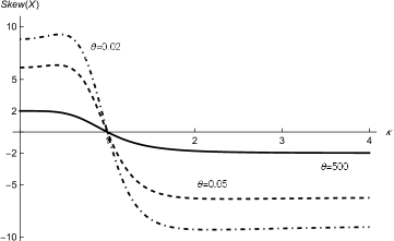
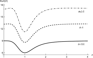
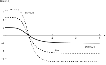
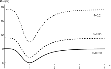
Figure 4 shows examples of behaviors of Skew(X)Skew𝑋\text{Skew}\left(X\right) and Kurt(X)Kurt𝑋\text{Kurt}\left(X\right), as functions of κ𝜅\kappa, at various levels of θ𝜃\theta.

Refer to caption
(a) Skewness
Refer to caption
(b) Kurtosis
Figure 4: Examples of behavior of Skew(X)Skew𝑋\text{Skew}\left(X\right) (on the left) and Kurt(X)Kurt𝑋\text{Kurt}\left(X\right) (on the right), as functions of κ𝜅\kappa, at various levels of θ𝜃\theta for the SE-AL distribution.

From Figure 4(a) we realize that: 1) large values of θ𝜃\theta tend to produce the plot of Skew(X)Skew𝑋\text{Skew}\left(X\right) we obtained for 𝒜(μ,β,κ)𝒜𝜇𝛽𝜅\mathcal{AL}\left(\mu,\beta,\kappa\right) (refer to Figure 1); and 2) as θ𝜃\theta decreases, the range of possible values of Skew(X)Skew𝑋\text{Skew}\left(X\right) increases. Moreover, to “significantly” modify the behavior of Skew(X)Skew𝑋\text{Skew}\left(X\right) with respect to the 𝒜(μ,β,κ)𝒜𝜇𝛽𝜅\mathcal{AL}\left(\mu,\beta,\kappa\right) case, we need low values of θ𝜃\theta (in the examples, θ=0.05𝜃0.05\theta=0.05 and θ=0.02𝜃0.02\theta=0.02). Similarly, from Figure 4(b) we realize that: 1) large values of θ𝜃\theta tend to produce the plot of Kurt(X)Kurt𝑋\text{Kurt}\left(X\right) we obtained for 𝒜(μ,β,κ)𝒜𝜇𝛽𝜅\mathcal{AL}\left(\mu,\beta,\kappa\right) (refer to Figure 1); and 2) κ𝜅\kappa kept fixed, the lower the value θ𝜃\theta, the higher the kurtosis. This means that the curve obtained for θ𝜃\theta\rightarrow\infty acts as a lower bound. Also in this case, to “significantly” modify the behavior of Kurt(X)Kurt𝑋\text{Kurt}\left(X\right) with respect to the 𝒜(μ,β,κ)𝒜𝜇𝛽𝜅\mathcal{AL}\left(\mu,\beta,\kappa\right) case, we need low values of θ𝜃\theta (in the examples, θ=1𝜃1\theta=1 and θ=0.5𝜃0.5\theta=0.5).

3.3 Unimodal gamma asymmetric Laplace distribution

Let

h(w;θ)=w1θewθθ1θ+1Γ(1θ+1),w>0,formulae-sequence𝑤𝜃superscript𝑤1𝜃superscript𝑒𝑤𝜃superscript𝜃1𝜃1Γ1𝜃1𝑤0h\left(w;\theta\right)=\frac{w^{\frac{1}{\theta}}e^{-\frac{w}{\theta}}}{\theta^{\frac{1}{\theta}+1}\Gamma\left(\frac{1}{\theta}+1\right)},\quad w>0, (32)

with θ>0𝜃0\theta>0, be the pdf of the unimodal gamma distribution (Chen, 2000) with mode in w=1𝑤1w=1. In symbols, W𝒰𝒢(θ)similar-to𝑊𝒰𝒢𝜃W\sim\mathcal{UG}\left(\theta\right); see also Bagnato & Punzo (2013). When the pdf in (32) is considered as mixing density in model (6), the pdf of the ALSM becomes

fALSM(x;μ,β,κ,θ)=1+θβκ1+κ2{[1+κθβ(xμ)]1θ2for xμ,[1+θβκ(μx)]1θ2for x<μ.subscript𝑓ALSM𝑥𝜇𝛽𝜅𝜃1𝜃𝛽𝜅1superscript𝜅2casessuperscriptdelimited-[]1𝜅𝜃𝛽𝑥𝜇1𝜃2for xμ,superscriptdelimited-[]1𝜃𝛽𝜅𝜇𝑥1𝜃2for x<μ.f_{\text{ALSM}}\left(x;\mu,\beta,\kappa,\theta\right)=\frac{1+\theta}{\beta}\frac{\kappa}{1+\kappa^{2}}\begin{cases}\left[1+\frac{\kappa\theta}{\beta}\left(x-\mu\right)\right]^{-\frac{1}{\theta}-2}&\text{for $x\geq\mu$,}\\[8.53581pt] \left[1+\frac{\theta}{\beta\kappa}\left(\mu-x\right)\right]^{-\frac{1}{\theta}-2}&\text{for $x<\mu$.}\end{cases} (33)

We refer to model (33) as unimodal gamma asymmetric Laplace (UG-AL) distribution. Model (33) reduces to 𝒜(μ,β,κ)𝒜𝜇𝛽𝜅\mathcal{AL}\left(\mu,\beta,\kappa\right) when θ0𝜃0\theta\rightarrow 0. Moreover, if κ=1𝜅1\kappa=1, then we obtain the UG-Laplace distribution, proposed by Punzo & Bagnato (2021a), as a special case.

If W𝒰𝒢(θ)similar-to𝑊𝒰𝒢𝜃W\sim\mathcal{UG}\left(\theta\right), then the r𝑟rth raw moment of 1/W1𝑊1/W is

E(1Wr)E1superscript𝑊𝑟\displaystyle\text{E}\left(\frac{1}{W^{r}}\right) =Γ(1θ+1r)θr1Γ(1θ),absentΓ1𝜃1𝑟superscript𝜃𝑟1Γ1𝜃\displaystyle=\frac{\Gamma\left(\frac{1}{\theta}+1-r\right)}{\theta^{r-1}\Gamma\left(\frac{1}{\theta}\right)},
=1j=1r(1+θjθ)absent1superscriptsubscriptproduct𝑗1𝑟1𝜃𝑗𝜃\displaystyle=\frac{1}{\displaystyle\prod_{j=1}^{r}\left(1+\theta-j\theta\right)} (34)

which exists if θ<1/(r1)𝜃1𝑟1\theta<1/(r-1). By substituting in (12)–(15) the first four raw moments in (34), mean, variance, skewness and kurtosis of the UG-AL distribution become

E(X)=μ+β(1κκ),E𝑋𝜇𝛽1𝜅𝜅\text{E}\left(X\right)=\mu+\beta\left(\frac{1}{\kappa}-\kappa\right), (35)
Var(X)=β2[θ(1κ2)2+κ4+1]κ2(1θ),Var𝑋superscript𝛽2delimited-[]𝜃superscript1superscript𝜅22superscript𝜅41superscript𝜅21𝜃\text{Var}\left(X\right)=\frac{\beta^{2}\left[\theta\left(1-\kappa^{2}\right)^{2}+\kappa^{4}+1\right]}{\kappa^{2}(1-\theta)}, (36)

which exists if 0<θ<10𝜃10<\theta<1,

Skew(X)=21θ(2θ+1)(1κ2)[θ(1κ2)2+κ4+κ2+1](2θ1)[θ(1κ2)2+κ4+1]3/2Skew𝑋21𝜃2𝜃11superscript𝜅2delimited-[]𝜃superscript1superscript𝜅22superscript𝜅4superscript𝜅212𝜃1superscriptdelimited-[]𝜃superscript1superscript𝜅22superscript𝜅4132\text{Skew}\left(X\right)=\frac{2\sqrt{1-\theta}(2\theta+1)\left(1-\kappa^{2}\right)\left[\theta\left(1-\kappa^{2}\right)^{2}+\kappa^{4}+\kappa^{2}+1\right]}{(2\theta-1)\left[\theta\left(1-\kappa^{2}\right)^{2}+\kappa^{4}+1\right]^{3/2}} (37)

which exists if 0<θ<1/20𝜃120<\theta<1/2, and

Kurt(X)=12(θ+1)κ84θκ6+[θ(6θ1)+1]κ44θκ2+θ+1[θ(6θ5)+1][θ(1κ2)2+κ4+1]23Kurt𝑋12𝜃1superscript𝜅84𝜃superscript𝜅6delimited-[]𝜃6𝜃11superscript𝜅44𝜃superscript𝜅2𝜃1delimited-[]𝜃6𝜃51superscriptdelimited-[]𝜃superscript1superscript𝜅22superscript𝜅4123\text{Kurt}\left(X\right)=12\frac{(\theta+1)\kappa^{8}-4\theta\kappa^{6}+\left[\theta(6\theta-1)+1\right]\kappa^{4}-4\theta\kappa^{2}+\theta+1}{\left[\theta(6\theta-5)+1\right]\left[\theta\left(1-\kappa^{2}\right)^{2}+\kappa^{4}+1\right]^{2}}-3 (38)

which exists if 0<θ<1/30𝜃130<\theta<1/3.

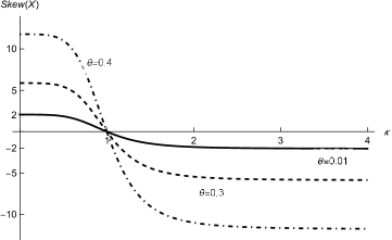
Figure 5 shows examples of behaviors of Skew(X)Skew𝑋\text{Skew}\left(X\right) and Kurt(X)Kurt𝑋\text{Kurt}\left(X\right), as functions of κ𝜅\kappa, at various levels of θ𝜃\theta.

Refer to caption
(a) Skewness
Refer to caption
(b) Kurtosis
Figure 5: Examples of behavior of Skew(X)Skew𝑋\text{Skew}\left(X\right) (on the left) and Kurt(X)Kurt𝑋\text{Kurt}\left(X\right) (on the right), as functions of κ𝜅\kappa, at various levels of θ𝜃\theta for the UG-AL distribution.

From Figure 5(a) we realize that: 1) small values of θ𝜃\theta tend to produce the plot of Skew(X)Skew𝑋\text{Skew}\left(X\right) we obtained for 𝒜(μ,β,κ)𝒜𝜇𝛽𝜅\mathcal{AL}\left(\mu,\beta,\kappa\right) (refer to Figure 1); and 2) as θ𝜃\theta grows from 0 to 1/2, the range of possible values of Skew(X)Skew𝑋\text{Skew}\left(X\right) increases. Similarly, from Figure 5(b) we realize that: 1) small values of θ𝜃\theta tend to produce the plot of Kurt(X)Kurt𝑋\text{Kurt}\left(X\right) we obtained for 𝒜(μ,β,κ)𝒜𝜇𝛽𝜅\mathcal{AL}\left(\mu,\beta,\kappa\right) (refer to Figure 1); and 2) κ𝜅\kappa kept fixed, as θ𝜃\theta grows from 0 to 1/3, the kurtosis increases. This means that the curve obtained for θ0𝜃0\theta\rightarrow 0 acts as a lower bound.

For completeness, and in analogy with the genesis of the t𝑡t distribution as a normal scale mixture, in A we give an alternative parameterization of the UG-AL distribution using a mixing gamma distribution with shape and rate equal to θ/2𝜃2\theta/2.

3.4 Inverse Gaussian asymmetric Laplace distribution

Let

h(w;θ)=3θ+12πθw3e(w3θ+1)22θw,w>0,formulae-sequence𝑤𝜃3𝜃12𝜋𝜃superscript𝑤3superscript𝑒superscript𝑤3𝜃122𝜃𝑤𝑤0h\left(w;\theta\right)=\sqrt{\frac{3\theta+1}{2\pi\theta w^{3}}}e^{-\frac{\left(w-\sqrt{3\theta+1}\right)^{2}}{2\theta w}},\quad w>0, (39)

with θ>0𝜃0\theta>0, be the pdf of the reparameterized inverse Gaussian distribution, introduced by Punzo (2019), with mode in w=1𝑤1w=1; see also Punzo et al. (2018). If W𝑊W has the pdf in (39), then we compactly write W𝒢(θ)similar-to𝑊𝒢𝜃W\sim\mathcal{IG}\left(\theta\right). When the pdf in (39) is considered as mixing density in model (6), the pdf of the ALSM becomes

fALSM(x;μ,β,κ,θ)=1+3θβκ1+κ2{e1+3θθ[11+2κθβ(xμ)]1+2κθβ(xμ)for xμ,e1+3θθ[11+2θβκ(μx)]1+2θβκ(μx)for x<μ.subscript𝑓ALSM𝑥𝜇𝛽𝜅𝜃13𝜃𝛽𝜅1superscript𝜅2casessuperscript𝑒13𝜃𝜃delimited-[]112𝜅𝜃𝛽𝑥𝜇12𝜅𝜃𝛽𝑥𝜇for xμ,superscript𝑒13𝜃𝜃delimited-[]112𝜃𝛽𝜅𝜇𝑥12𝜃𝛽𝜅𝜇𝑥for x<μ.f_{\text{ALSM}}\left(x;\mu,\beta,\kappa,\theta\right)=\frac{\sqrt{1+3\theta}}{\beta}\frac{\kappa}{1+\kappa^{2}}\begin{cases}\displaystyle\frac{e^{\frac{\sqrt{1+3\theta}}{\theta}\left[1-\sqrt{1+2\frac{\kappa\theta}{\beta}\left(x-\mu\right)}\right]}}{\sqrt{1+2\frac{\kappa\theta}{\beta}\left(x-\mu\right)}}&\text{for $x\geq\mu$,}\\[17.07164pt] \displaystyle\frac{e^{\frac{\sqrt{1+3\theta}}{\theta}\left[1-\sqrt{1+2\frac{\theta}{\beta\kappa}\left(\mu-x\right)}\right]}}{\sqrt{1+2\frac{\theta}{\beta\kappa}\left(\mu-x\right)}}&\text{for $x<\mu$.}\end{cases} (40)

We call inverse Gaussian asymmetric Laplace (IG-AL) the resulting distribution. Model (40) reduces to 𝒜(μ,β,κ)𝒜𝜇𝛽𝜅\mathcal{AL}\left(\mu,\beta,\kappa\right) when θ0𝜃0\theta\rightarrow 0. Moreover, if κ=1𝜅1\kappa=1, then we obtain the IG-Laplace distribution, proposed by Punzo & Bagnato (2021a), as a special case.

When W𝒢(θ)similar-to𝑊𝒢𝜃W\sim\mathcal{IG}\left(\theta\right), the r𝑟rth raw moment of 1/W1𝑊1/W is

E(1Wr)=2θπ(3θ+1)12r4e3θ+1θK12+r(3θ+1θ),E1superscript𝑊𝑟2𝜃𝜋superscript3𝜃112𝑟4superscript𝑒3𝜃1𝜃subscript𝐾12𝑟3𝜃1𝜃\text{E}\left(\frac{1}{W^{r}}\right)=\sqrt{\frac{2}{\theta\pi}}\left(3\theta+1\right)^{\frac{1-2r}{4}}e^{\frac{\sqrt{3\theta+1}}{\theta}}K_{\frac{1}{2}+r}\left(\frac{\sqrt{3\theta+1}}{\theta}\right), (41)

where Kλ(x)subscript𝐾𝜆𝑥K_{\lambda}\left(x\right) is the modified Bessel function of the third kind; for details, see Abramowitz & Stegun (1965) and Watson (1995). By substituting in (12)–(15) the first four raw moments in (41), mean, variance, skewness and kurtosis of the IG-AL distribution become

E(X)=μ+β(1κκ)θ+3θ+13θ+1,E𝑋𝜇𝛽1𝜅𝜅𝜃3𝜃13𝜃1\text{E}\left(X\right)=\mu+\beta\left(\frac{1}{\kappa}-\kappa\right)\frac{\theta+\sqrt{3\theta+1}}{3\theta+1}, (42)
Var(X)=β2κ2(3θ+1)[2(3θ23θ+1+3θ3θ+1+1)(κ6+1)(κ2+1)(θ3θ+1+1)2(1κ4)2(κ2+1)2],Var𝑋superscript𝛽2superscript𝜅23𝜃1delimited-[]23superscript𝜃23𝜃13𝜃3𝜃11superscript𝜅61superscript𝜅21superscript𝜃3𝜃112superscript1superscript𝜅42superscriptsuperscript𝜅212\text{Var}\left(X\right)=\frac{\beta^{2}}{\kappa^{2}(3\theta+1)}\left[\frac{2\left(\frac{3\theta^{2}}{3\theta+1}+\frac{3\theta}{\sqrt{3\theta+1}}+1\right)\left(\kappa^{6}+1\right)}{\left(\kappa^{2}+1\right)}-\frac{\left(\frac{\theta}{\sqrt{3\theta+1}}+1\right)^{2}\left(1-\kappa^{4}\right)^{2}}{\left(\kappa^{2}+1\right)^{2}}\right], (43)
Skew(X)=Skew𝑋absent\displaystyle\text{Skew}\left(X\right)= 2(1κ2)(θ2(5κ44κ2+5)+θ((43θ+1+3)κ423θ+1κ2+43θ+1+3)+κ4+1)3/221superscript𝜅2superscriptsuperscript𝜃25superscript𝜅44superscript𝜅25𝜃43𝜃13superscript𝜅423𝜃1superscript𝜅243𝜃13superscript𝜅4132\displaystyle\frac{2\left(1-\kappa^{2}\right)}{\left(\theta^{2}\left(5\kappa^{4}-4\kappa^{2}+5\right)+\theta\left(\left(4\sqrt{3\theta+1}+3\right)\kappa^{4}-2\sqrt{3\theta+1}\kappa^{2}+4\sqrt{3\theta+1}+3\right)+\kappa^{4}+1\right)^{3/2}}
×{θ3(37κ4+7κ2+37)+3θ2[(103θ+1+9)κ4+(43θ+1+6)κ2+103θ+1+9]+\displaystyle\times\bigg{\{}\theta^{3}\left(37\kappa^{4}+7\kappa^{2}+37\right)+3\theta^{2}\left[\left(10\sqrt{3\theta+1}+9\right)\kappa^{4}+\left(4\sqrt{3\theta+1}+6\right)\kappa^{2}+10\sqrt{3\theta+1}+9\right]+
+3θ[(3θ+1+3)κ4+(3θ+1+2)κ2+3θ+1+3]+3θ+1(κ4+κ2+1)}\displaystyle+3\theta\left[\left(\sqrt{3\theta+1}+3\right)\kappa^{4}+\left(\sqrt{3\theta+1}+2\right)\kappa^{2}+\sqrt{3\theta+1}+3\right]+\sqrt{3\theta+1}\left(\kappa^{4}+\kappa^{2}+1\right)\bigg{\}} (44)

and

Kurt(X)=Kurt𝑋absent\displaystyle\text{Kurt}\left(X\right)= 12(3θ+1)4(κ2+1)2[(θ+3θ+1)2(κ21)2(3θ+1)22{3θ+1+3θ[3θ+1+θ(3θ+1+3)+1]}(κ4κ2+1)(3θ+1)5/2]212superscript3𝜃14superscriptsuperscript𝜅212superscriptdelimited-[]superscript𝜃3𝜃12superscriptsuperscript𝜅212superscript3𝜃1223𝜃13𝜃delimited-[]3𝜃1𝜃3𝜃131superscript𝜅4superscript𝜅21superscript3𝜃1522\displaystyle\frac{12}{(3\theta+1)^{4}\left(\kappa^{2}+1\right)^{2}\left[\frac{\left(\theta+\sqrt{3\theta+1}\right)^{2}\left(\kappa^{2}-1\right)^{2}}{(3\theta+1)^{2}}-\frac{2\left\{\sqrt{3\theta+1}+3\theta\left[\sqrt{3\theta+1}+\theta\left(\sqrt{3\theta+1}+3\right)+1\right]\right\}\left(\kappa^{4}-\kappa^{2}+1\right)}{(3\theta+1)^{5/2}}\right]^{2}}
×[2(105θ4+135θ3+105θ33θ+1+54θ2+10θ(3θ+1)3/2+6θ+1)(κ2+1)(κ10+1)+\displaystyle\times\bigg{[}2\left(105\theta^{4}+135\theta^{3}+105\theta^{3}\sqrt{3\theta+1}+54\theta^{2}+10\theta(3\theta+1)^{3/2}+6\theta+1\right)\left(\kappa^{2}+1\right)\left(\kappa^{10}+1\right)+
+[3θ(θ+3θ+1+1)+1]2(κ6+1)2+limit-fromsuperscriptdelimited-[]3𝜃𝜃3𝜃1112superscriptsuperscript𝜅612\displaystyle+\left[3\theta\left(\theta+\sqrt{3\theta+1}+1\right)+1\right]^{2}\left(\kappa^{6}+1\right)^{2}+
2(θ+3θ+1){3θ+1+3θ[3θ+1+θ(5θ+53θ+1+6)+2]}(κ4+1)(κ41)2]3\displaystyle-2\left(\theta+\sqrt{3\theta+1}\right)\left\{\sqrt{3\theta+1}+3\theta\left[\sqrt{3\theta+1}+\theta\left(5\theta+5\sqrt{3\theta+1}+6\right)+2\right]\right\}\left(\kappa^{4}+1\right)\left(\kappa^{4}-1\right)^{2}\bigg{]}-3 (45)

Figure 6 shows examples of behaviors of Skew(X)Skew𝑋\text{Skew}\left(X\right) and Kurt(X)Kurt𝑋\text{Kurt}\left(X\right), as functions of κ𝜅\kappa, at various levels of θ𝜃\theta.

Refer to caption
(a) Skewness
Refer to caption
(b) Kurtosis
Figure 6: Examples of behavior of Skew(X)Skew𝑋\text{Skew}\left(X\right) (on the left) and Kurt(X)Kurt𝑋\text{Kurt}\left(X\right) (on the right), as functions of κ𝜅\kappa, at various levels of θ𝜃\theta for the IG-AL distribution.

From Figure 6(a) we realize that: 1) small values of θ𝜃\theta tend to produce the plot of Skew(X)Skew𝑋\text{Skew}\left(X\right) we obtained for 𝒜(μ,β,κ)𝒜𝜇𝛽𝜅\mathcal{AL}\left(\mu,\beta,\kappa\right) (refer to Figure 1); and 2) as θ𝜃\theta grows, the range of possible values of Skew(X)Skew𝑋\text{Skew}\left(X\right) increases. Similarly, from Figure 6(b) we realize that: 1) small values of θ𝜃\theta tend to produce the plot of Kurt(X)Kurt𝑋\text{Kurt}\left(X\right) we obtained for 𝒜(μ,β,κ)𝒜𝜇𝛽𝜅\mathcal{AL}\left(\mu,\beta,\kappa\right) (refer to Figure 1); and 2) κ𝜅\kappa kept fixed, as θ𝜃\theta grows, the kurtosis increases. This means that the curve obtained for θ0𝜃0\theta\rightarrow 0 acts as a lower bound.

3.5 Power-function asymmetric Laplace distribution

Let

h(w;θ)=θwθ1,0<w<1,formulae-sequence𝑤𝜃𝜃superscript𝑤𝜃10𝑤1h\left(w;\theta\right)=\theta w^{\theta-1},\quad 0<w<1, (46)

with shape parameter θ>0𝜃0\theta>0, be the pdf of the (standard) power-function distribution, in symbols W𝒫(θ)similar-to𝑊𝒫𝜃W\sim\mathcal{PF}\left(\theta\right), special case of the beta distribution (θ,1)𝜃1\mathcal{B}\left(\theta,1\right); see Johnson & Kotz (1970a, Chapter 25) and Ahsanullah & Kabir (1974). When the pdf in (46) is considered as mixing density in model (6), the pdf of the ALSM simplifies as

fALSM(x;μ,β,κ,θ)=θβκ1+κ2{[κβ(xμ)](θ+1)γ[θ+1,κβ(xμ)]for xμ,[1βκ(μx)](θ+1)γ[θ+1,1βκ(μx)]for x<μ,subscript𝑓ALSM𝑥𝜇𝛽𝜅𝜃𝜃𝛽𝜅1superscript𝜅2casessuperscriptdelimited-[]𝜅𝛽𝑥𝜇𝜃1𝛾𝜃1𝜅𝛽𝑥𝜇for xμsuperscriptdelimited-[]1𝛽𝜅𝜇𝑥𝜃1𝛾𝜃11𝛽𝜅𝜇𝑥for x<μf_{\text{ALSM}}\left(x;\mu,\beta,\kappa,\theta\right)=\frac{\theta}{\beta}\frac{\kappa}{1+\kappa^{2}}\begin{cases}\left[\frac{\kappa}{\beta}\left(x-\mu\right)\right]^{-\left(\theta+1\right)}\gamma\left[\theta+1,\frac{\kappa}{\beta}\left(x-\mu\right)\right]&\text{for $x\geq\mu$},\\[14.22636pt] \left[\frac{1}{\beta\kappa}\left(\mu-x\right)\right]^{-\left(\theta+1\right)}\gamma\left[\theta+1,\frac{1}{\beta\kappa}\left(\mu-x\right)\right]&\text{for $x<\mu$},\end{cases} (47)

where γ(s,x)=0xts1et𝑑t𝛾𝑠𝑥superscriptsubscript0𝑥superscript𝑡𝑠1superscript𝑒𝑡differential-d𝑡\gamma\left(s,x\right)=\int_{0}^{x}t^{s-1}e^{-t}dt is the lower incomplete gamma function. We refer to the resulting distribution as power-function asymmetric Laplace (PF-AL). Model (47) reduces to 𝒜(μ,β,κ)𝒜𝜇𝛽𝜅\mathcal{AL}\left(\mu,\beta,\kappa\right) when θ𝜃\theta\rightarrow\infty. Moreover, if κ=1𝜅1\kappa=1, then we obtain the PF-Laplace distribution, proposed by Punzo & Bagnato (2021a), as a special case.

When W𝒫(θ)similar-to𝑊𝒫𝜃W\sim\mathcal{PF}\left(\theta\right), the r𝑟rth raw moment of 1/W1𝑊1/W – to be substituted in (12)–(15) to obtain mean, variance, skewness and kurtosis of the PF-AL distribution – is

E(1Wr)=θθr,E1superscript𝑊𝑟𝜃𝜃𝑟\text{E}\left(\frac{1}{W^{r}}\right)=\frac{\theta}{\theta-r}, (48)

which exists for θ>r𝜃𝑟\theta>r. Thanks to (48), we have

E(X)=μ+β(1κκ)θθ1,E𝑋𝜇𝛽1𝜅𝜅𝜃𝜃1\text{E}\left(X\right)=\mu+\beta\left(\frac{1}{\kappa}-\kappa\right)\frac{\theta}{\theta-1}, (49)

which exists if θ>1𝜃1\theta>1,

Var(X)=β2θ[(θ2)θ(κ4+1)+2(κ4κ2+1)](θ2)(θ1)2κ2,Var𝑋superscript𝛽2𝜃delimited-[]𝜃2𝜃superscript𝜅412superscript𝜅4superscript𝜅21𝜃2superscript𝜃12superscript𝜅2\text{Var}\left(X\right)=\frac{\beta^{2}\theta\left[(\theta-2)\theta\left(\kappa^{4}+1\right)+2\left(\kappa^{4}-\kappa^{2}+1\right)\right]}{(\theta-2)(\theta-1)^{2}\kappa^{2}}, (50)

which exists if θ>2𝜃2\theta>2,

Skew(X)=2θ2θ(κ21){[(θ2)θ((θ3)θ+6)+6]κ4+(θ3)θ((θ2)θ+3)κ2+(θ2)θ((θ3)θ+6)+6}(θ3)[(θ2)θ(κ4+1)+2(κ4κ2+1)]3/2Skew𝑋2𝜃2𝜃superscript𝜅21delimited-[]𝜃2𝜃𝜃3𝜃66superscript𝜅4𝜃3𝜃𝜃2𝜃3superscript𝜅2𝜃2𝜃𝜃3𝜃66𝜃3superscriptdelimited-[]𝜃2𝜃superscript𝜅412superscript𝜅4superscript𝜅2132\text{Skew}\left(X\right)=-\frac{2\sqrt{\frac{\theta-2}{\theta}}\left(\kappa^{2}-1\right)\left\{\left[(\theta-2)\theta((\theta-3)\theta+6)+6\right]\kappa^{4}+(\theta-3)\theta((\theta-2)\theta+3)\kappa^{2}+(\theta-2)\theta((\theta-3)\theta+6)+6\right\}}{(\theta-3)\left[(\theta-2)\theta\left(\kappa^{4}+1\right)+2\left(\kappa^{4}-\kappa^{2}+1\right)\right]^{3/2}} (51)

which exists if θ>3𝜃3\theta>3, and

Kurt(X)=12(θ2)2(θ1)4[θ(κ6+1)2(θ2)22θ(κ4+1)(κ41)2(θ3)(θ1)+2(κ2+1)(κ10+1)θ4]θ(κ2+1)2[(θ2)θ(κ4+1)+2(κ4κ2+1)]23,Kurt𝑋12superscript𝜃22superscript𝜃14delimited-[]𝜃superscriptsuperscript𝜅612superscript𝜃222𝜃superscript𝜅41superscriptsuperscript𝜅412𝜃3𝜃12superscript𝜅21superscript𝜅101𝜃4𝜃superscriptsuperscript𝜅212superscriptdelimited-[]𝜃2𝜃superscript𝜅412superscript𝜅4superscript𝜅2123\text{Kurt}\left(X\right)=\frac{12(\theta-2)^{2}(\theta-1)^{4}\left[\frac{\theta\left(\kappa^{6}+1\right)^{2}}{(\theta-2)^{2}}-\frac{2\theta\left(\kappa^{4}+1\right)\left(\kappa^{4}-1\right)^{2}}{(\theta-3)(\theta-1)}+\frac{2\left(\kappa^{2}+1\right)\left(\kappa^{10}+1\right)}{\theta-4}\right]}{\theta\left(\kappa^{2}+1\right)^{2}\left[(\theta-2)\theta\left(\kappa^{4}+1\right)+2\left(\kappa^{4}-\kappa^{2}+1\right)\right]^{2}}-3, (52)

which exists if θ>4𝜃4\theta>4.

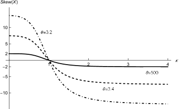
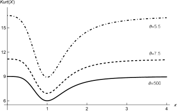
Figure 7 shows examples of behaviors of Skew(X)Skew𝑋\text{Skew}\left(X\right) and Kurt(X)Kurt𝑋\text{Kurt}\left(X\right), as functions of κ𝜅\kappa, at various levels of θ𝜃\theta.

Refer to caption
(a) Skewness
Refer to caption
(b) Kurtosis
Figure 7: Examples of behavior of Skew(X)Skew𝑋\text{Skew}\left(X\right) (on the left) and Kurt(X)Kurt𝑋\text{Kurt}\left(X\right) (on the right), as functions of κ𝜅\kappa, at various levels of θ𝜃\theta for the PF-AL distribution.

From Figure 7(a) we realize that: 1) large values of θ𝜃\theta tend to produce the plot of Skew(X)Skew𝑋\text{Skew}\left(X\right) we obtained for 𝒜(μ,β,κ)𝒜𝜇𝛽𝜅\mathcal{AL}\left(\mu,\beta,\kappa\right) (refer to Figure 1); and 2) as θ𝜃\theta decreases (to a minimum value of 3), the range of possible values of Skew(X)Skew𝑋\text{Skew}\left(X\right) increases. Moreover, to “significantly” modify the behavior of Skew(X)Skew𝑋\text{Skew}\left(X\right) with respect to the 𝒜(μ,β,κ)𝒜𝜇𝛽𝜅\mathcal{AL}\left(\mu,\beta,\kappa\right) case, we need low values of θ𝜃\theta (in the examples, θ=3.4𝜃3.4\theta=3.4 and θ=3.2𝜃3.2\theta=3.2). Similarly, from Figure 7(b) we realize that: 1) large values of θ𝜃\theta tend to produce the plot of Kurt(X)Kurt𝑋\text{Kurt}\left(X\right) we obtained for 𝒜(μ,β,κ)𝒜𝜇𝛽𝜅\mathcal{AL}\left(\mu,\beta,\kappa\right) (refer to Figure 1); and 2) κ𝜅\kappa kept fixed, the lower the value θ𝜃\theta (with a minimum of 4), the higher the kurtosis. This means that the curve obtained for θ𝜃\theta\rightarrow\infty acts as a lower bound. Also in this case, to “significantly” modify the behavior of Kurt(X)Kurt𝑋\text{Kurt}\left(X\right) with respect to the 𝒜(μ,β,κ)𝒜𝜇𝛽𝜅\mathcal{AL}\left(\mu,\beta,\kappa\right) case, we need low values of θ𝜃\theta (in the examples, θ=7.5𝜃7.5\theta=7.5 and θ=5.5𝜃5.5\theta=5.5).

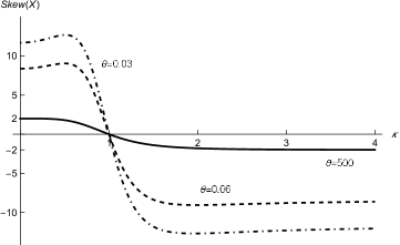
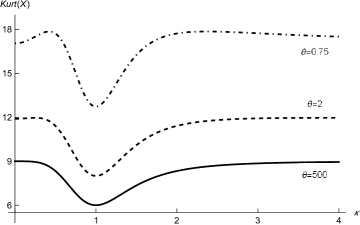
3.6 Pareto asymmetric Laplace distribution

Let

h(w;θ)=θxθ+1,w>1,formulae-sequence𝑤𝜃𝜃superscript𝑥𝜃1𝑤1h\left(w;\theta\right)=\frac{\theta}{x^{\theta+1}},\quad w>1, (53)

with θ>0𝜃0\theta>0, be the pdf of a Pareto distribution with unitary scale and shape θ𝜃\theta; in symbols, W𝒫(θ)similar-to𝑊𝒫𝜃W\sim\mathcal{P}\left(\theta\right). When the pdf in (53) is considered as mixing density in model (6), the pdf of the ALSM simplifies as

fALSM(x;μ,β,κ,θ)=θβκ1+κ2{Eθ[κβ(xμ)]for xμ,Eθ[1βκ(μx)]for x<μ.subscript𝑓ALSM𝑥𝜇𝛽𝜅𝜃𝜃𝛽𝜅1superscript𝜅2casessubscript𝐸𝜃delimited-[]𝜅𝛽𝑥𝜇for xμ,subscript𝐸𝜃delimited-[]1𝛽𝜅𝜇𝑥for x<μ.f_{\text{ALSM}}\left(x;\mu,\beta,\kappa,\theta\right)=\frac{\theta}{\beta}\frac{\kappa}{1+\kappa^{2}}\begin{cases}E_{\theta}\left[\frac{\kappa}{\beta}\left(x-\mu\right)\right]&\text{for $x\geq\mu$,}\\[14.22636pt] E_{\theta}\left[\frac{1}{\beta\kappa}\left(\mu-x\right)\right]&\text{for $x<\mu$.}\end{cases} (54)

We refer to the resulting distribution as Pareto asymmetric Laplace (P-AL). Model (54) reduces to 𝒜(μ,β,κ)𝒜𝜇𝛽𝜅\mathcal{AL}\left(\mu,\beta,\kappa\right) when θ𝜃\theta\rightarrow\infty.

When W𝒫(θ)similar-to𝑊𝒫𝜃W\sim\mathcal{P}\left(\theta\right), the r𝑟rth raw moment of 1/W1𝑊1/W is

E(1Wr)=θθ+r.E1superscript𝑊𝑟𝜃𝜃𝑟\text{E}\left(\frac{1}{W^{r}}\right)=\frac{\theta}{\theta+r}. (55)

By substituting in (12)–(15) the first four raw moments in (55), mean, variance, skewness and kurtosis of the P-AL distribution become

E(X)=μ+β(1κκ)θ1+θ,E𝑋𝜇𝛽1𝜅𝜅𝜃1𝜃\text{E}\left(X\right)=\mu+\beta\left(\frac{1}{\kappa}-\kappa\right)\frac{\theta}{1+\theta}, (56)
Var(X)=β2θ[(θ+2)(1+κ4)2κ2](θ+1)2κ2,Var𝑋superscript𝛽2𝜃delimited-[]𝜃21superscript𝜅42superscript𝜅2superscript𝜃12superscript𝜅2\text{Var}\left(X\right)=\frac{\beta^{2}\theta\left[\left(\theta+2\right)\left(1+\kappa^{4}\right)-2\kappa^{2}\right]}{(\theta+1)^{2}\kappa^{2}}, (57)
Skew(X)=Skew𝑋absent\displaystyle\text{Skew}\left(X\right)= 1(θ+3)[θ2(κ4+1)+2θ(κ4+1)+2(κ4κ2+1)]3/2{2θ+2θ(1κ2)[θ4(κ4+κ2+1)+\displaystyle\frac{1}{(\theta+3)\left[\theta^{2}\left(\kappa^{4}+1\right)+2\theta\left(\kappa^{4}+1\right)+2\left(\kappa^{4}-\kappa^{2}+1\right)\right]^{3/2}}\Bigg{\{}2\sqrt{\frac{\theta+2}{\theta}}\left(1-\kappa^{2}\right)\bigg{[}\theta^{4}\left(\kappa^{4}+\kappa^{2}+1\right)+
+5θ3(κ4+κ2+1)+3θ2(4κ4+3κ2+4)+3θ(4κ4+3κ2+4)+6(κ4+1)]}\displaystyle+5\theta^{3}\left(\kappa^{4}+\kappa^{2}+1\right)+3\theta^{2}\left(4\kappa^{4}+3\kappa^{2}+4\right)+3\theta\left(4\kappa^{4}+3\kappa^{2}+4\right)+6\left(\kappa^{4}+1\right)\bigg{]}\Bigg{\}} (58)

and

Kurt(X)=12(θ+1)4(θ+2)2[θ(κ6+1)2(θ+2)22θ(κ4+1)(κ41)2(θ+1)(θ+3)+2(κ2+1)(κ10+1)θ+4]θ[θ2(κ2+1)(κ4+1)+2θ(κ2+1)(κ4+1)+2κ6+2]23Kurt𝑋12superscript𝜃14superscript𝜃22delimited-[]𝜃superscriptsuperscript𝜅612superscript𝜃222𝜃superscript𝜅41superscriptsuperscript𝜅412𝜃1𝜃32superscript𝜅21superscript𝜅101𝜃4𝜃superscriptdelimited-[]superscript𝜃2superscript𝜅21superscript𝜅412𝜃superscript𝜅21superscript𝜅412superscript𝜅6223\text{Kurt}\left(X\right)=\frac{12(\theta+1)^{4}(\theta+2)^{2}\left[\frac{\theta\left(\kappa^{6}+1\right)^{2}}{(\theta+2)^{2}}-\frac{2\theta\left(\kappa^{4}+1\right)\left(\kappa^{4}-1\right)^{2}}{(\theta+1)(\theta+3)}+\frac{2\left(\kappa^{2}+1\right)\left(\kappa^{10}+1\right)}{\theta+4}\right]}{\theta\left[\theta^{2}\left(\kappa^{2}+1\right)\left(\kappa^{4}+1\right)+2\theta\left(\kappa^{2}+1\right)\left(\kappa^{4}+1\right)+2\kappa^{6}+2\right]^{2}}-3 (59)

Figure 8 shows examples of behaviors of Skew(X)Skew𝑋\text{Skew}\left(X\right) and Kurt(X)Kurt𝑋\text{Kurt}\left(X\right), as functions of κ𝜅\kappa, at various levels of θ𝜃\theta.

Refer to caption
(a) Skewness
Refer to caption
(b) Kurtosis
Figure 8: Examples of behavior of Skew(X)Skew𝑋\text{Skew}\left(X\right) (on the left) and Kurt(X)Kurt𝑋\text{Kurt}\left(X\right) (on the right), as functions of κ𝜅\kappa, at various levels of θ𝜃\theta for the P-AL distribution.

From Figure 8(a) we realize that: 1) a large value of θ𝜃\theta produces, as a limiting case, the plot of Skew(X)Skew𝑋\text{Skew}\left(X\right) we obtained for 𝒜(μ,β,κ)𝒜𝜇𝛽𝜅\mathcal{AL}\left(\mu,\beta,\kappa\right) (refer to Figure 1); and 2) as θ𝜃\theta decreases, the range of possible values of Skew(X)Skew𝑋\text{Skew}\left(X\right) increases. Moreover, to “significantly” modify the behavior of Skew(X)Skew𝑋\text{Skew}\left(X\right) with respect to the 𝒜(μ,β,κ)𝒜𝜇𝛽𝜅\mathcal{AL}\left(\mu,\beta,\kappa\right) case, we need low values of θ𝜃\theta (in the examples, θ=0.06𝜃0.06\theta=0.06 and θ=0.03𝜃0.03\theta=0.03). Similarly, from Figure 8(b) we realize that: 1) a large value of θ𝜃\theta produces, as a limiting case, the plot of Kurt(X)Kurt𝑋\text{Kurt}\left(X\right) we obtained for 𝒜(μ,β,κ)𝒜𝜇𝛽𝜅\mathcal{AL}\left(\mu,\beta,\kappa\right) (refer to Figure 1); and 2) κ𝜅\kappa kept fixed, the lower the value θ𝜃\theta, the higher the kurtosis. This means that the curve obtained for θ𝜃\theta\rightarrow\infty acts as a lower bound. Also in this case, to “significantly” modify the behavior of Kurt(X)Kurt𝑋\text{Kurt}\left(X\right) with respect to the 𝒜(μ,β,κ)𝒜𝜇𝛽𝜅\mathcal{AL}\left(\mu,\beta,\kappa\right) case, we need low values of θ𝜃\theta (in the examples, θ=2𝜃2\theta=2 and θ=0.75𝜃0.75\theta=0.75).

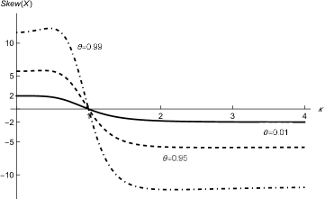
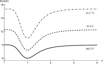
3.7 Uniform asymmetric Laplace distribution

When a uniform distribution on (1θ,1)1𝜃1\left(1-\theta,1\right), 0<θ<10𝜃10<\theta<1, is chosen as mixing distribution, in symbols W𝒰(1θ,1)(θ)similar-to𝑊subscript𝒰1𝜃1𝜃W\sim\mathcal{U}_{\left(1-\theta,1\right)}\left(\theta\right), the pdf of the ALSM becomes

fALSM(x;μ,β,κ,θ)=κθ(1+κ2)(xμ)2{1κeκ(θ1)(xμ)β{(βκ+xμ)[1eκθ(xμ)β]θ(xμ)}for xμ,κe(θ1)(μx)βκ{(βκ+μx)[1eθ(μx)βκ]θ(μx)}for x<μ.subscript𝑓ALSM𝑥𝜇𝛽𝜅𝜃𝜅𝜃1superscript𝜅2superscript𝑥𝜇2cases1𝜅superscript𝑒𝜅𝜃1𝑥𝜇𝛽𝛽𝜅𝑥𝜇delimited-[]1superscript𝑒𝜅𝜃𝑥𝜇𝛽𝜃𝑥𝜇for xμ,𝜅superscript𝑒𝜃1𝜇𝑥𝛽𝜅𝛽𝜅𝜇𝑥delimited-[]1superscript𝑒𝜃𝜇𝑥𝛽𝜅𝜃𝜇𝑥for x<μ.f_{\text{ALSM}}\left(x;\mu,\beta,\kappa,\theta\right)=\frac{\kappa}{\theta\left(1+\kappa^{2}\right)\left(x-\mu\right)^{2}}\begin{cases}\frac{1}{\kappa}e^{\frac{\kappa(\theta-1)(x-\mu)}{\beta}}\left\{\left(\frac{\beta}{\kappa}+x-\mu\right)\left[1-e^{-\frac{\kappa\theta(x-\mu)}{\beta}}\right]-\theta\left(x-\mu\right)\right\}&\text{for $x\geq\mu$,}\\[14.22636pt] \kappa e^{\frac{(\theta-1)(\mu-x)}{\beta\kappa}}\left\{\left(\beta\kappa+\mu-x\right)\left[1-e^{-\frac{\theta(\mu-x)}{\beta\kappa}}\right]-\theta\left(\mu-x\right)\right\}&\text{for $x<\mu$.}\end{cases} (60)

We will refer to the resulting distribution as uniform asymmetric Laplace (U-AL) or, in analogy with Punzo & Bagnato (2021b), as tail-inflated asymmetric Laplace distribution. Model (60) reduces to 𝒜(μ,β,κ)𝒜𝜇𝛽𝜅\mathcal{AL}\left(\mu,\beta,\kappa\right) when θ0𝜃0\theta\rightarrow 0.

When W𝒰(1θ,1)(θ)similar-to𝑊subscript𝒰1𝜃1𝜃W\sim\mathcal{U}_{\left(1-\theta,1\right)}\left(\theta\right), the r𝑟rth raw moment of 1/W1𝑊1/W is

E(1Wr)={log(1θ)θfor r=1,(1θ)1r1θ(r1)for r{2,3,}.E1superscript𝑊𝑟cases1𝜃𝜃for r=1,superscript1𝜃1𝑟1𝜃𝑟1for r{2,3,}.\text{E}\left(\frac{1}{W^{r}}\right)=\begin{cases}-\displaystyle\frac{\log\left(1-\theta\right)}{\theta}&\text{for $r=1$,}\\[5.69054pt] \displaystyle\frac{\left(1-\theta\right)^{1-r}-1}{\theta\left(r-1\right)}&\text{for $r\in\{2,3,\ldots\}$.}\end{cases} (61)

By substituting in (12)–(15) the first four raw moments in (61), mean, variance, skewness and kurtosis of the U-AL distribution become

E(X)=μβ(1κκ)log(1θ)θ,E𝑋𝜇𝛽1𝜅𝜅1𝜃𝜃\text{E}\left(X\right)=\mu-\beta\left(\frac{1}{\kappa}-\kappa\right)\frac{\log(1-\theta)}{\theta}, (62)
Var(X)=β2θ2κ2log(1θ)[(κ21)2log(1θ)+2θ(κ4κ2+1)],Var𝑋superscript𝛽2superscript𝜃2superscript𝜅21𝜃delimited-[]superscriptsuperscript𝜅2121𝜃2𝜃superscript𝜅4superscript𝜅21\text{Var}\left(X\right)=-\frac{\beta^{2}}{\theta^{2}\kappa^{2}}\log(1-\theta)\left[\left(\kappa^{2}-1\right)^{2}\log(1-\theta)+2\theta\left(\kappa^{4}-\kappa^{2}+1\right)\right], (63)
Skew(X)=3[1(θ1)21]θ2(κ2+1)2(1κ8)+6θ2(κ2+1)(1κ4)(κ6+1)log(1θ)1θ+2(κ41)3log3(1θ)θ3(κ2+1)3[(κ21)2log2(1θ)θ22(κ4κ2+1)θ1]3/2Skew𝑋3delimited-[]1superscript𝜃121superscript𝜃2superscriptsuperscript𝜅2121superscript𝜅86superscript𝜃2superscript𝜅211superscript𝜅4superscript𝜅611𝜃1𝜃2superscriptsuperscript𝜅413superscript31𝜃superscript𝜃3superscriptsuperscript𝜅213superscriptdelimited-[]superscriptsuperscript𝜅212superscript21𝜃superscript𝜃22superscript𝜅4superscript𝜅21𝜃132\text{Skew}\left(X\right)=\frac{3\left[\frac{1}{(\theta-1)^{2}}-1\right]\theta^{2}\left(\kappa^{2}+1\right)^{2}\left(1-\kappa^{8}\right)+\frac{6\theta^{2}\left(\kappa^{2}+1\right)\left(1-\kappa^{4}\right)\left(\kappa^{6}+1\right)\log(1-\theta)}{1-\theta}+2\left(\kappa^{4}-1\right)^{3}\log^{3}(1-\theta)}{\theta^{3}\left(\kappa^{2}+1\right)^{3}\left[-\frac{\left(\kappa^{2}-1\right)^{2}\log^{2}(1-\theta)}{\theta^{2}}-\frac{2\left(\kappa^{4}-\kappa^{2}+1\right)}{\theta-1}\right]^{3/2}} (64)

and

Kurt(X)=4{3θ(κ6+1)2(θ1)23(θ2)(κ4+1)(κ41)2log(1θ)(θ1)2+2[1(1θ)31](κ2+1)(κ10+1)}θ(κ2+1)2[(κ21)2log2(1θ)θ2+2(κ4κ2+1)θ1]23Kurt𝑋43𝜃superscriptsuperscript𝜅612superscript𝜃123𝜃2superscript𝜅41superscriptsuperscript𝜅4121𝜃superscript𝜃122delimited-[]1superscript1𝜃31superscript𝜅21superscript𝜅101𝜃superscriptsuperscript𝜅212superscriptdelimited-[]superscriptsuperscript𝜅212superscript21𝜃superscript𝜃22superscript𝜅4superscript𝜅21𝜃123\text{Kurt}\left(X\right)=\frac{4\left\{\frac{3\theta\left(\kappa^{6}+1\right)^{2}}{(\theta-1)^{2}}-\frac{3(\theta-2)\left(\kappa^{4}+1\right)\left(\kappa^{4}-1\right)^{2}\log(1-\theta)}{(\theta-1)^{2}}+2\left[\frac{1}{(1-\theta)^{3}}-1\right]\left(\kappa^{2}+1\right)\left(\kappa^{10}+1\right)\right\}}{\theta\left(\kappa^{2}+1\right)^{2}\left[\frac{\left(\kappa^{2}-1\right)^{2}\log^{2}(1-\theta)}{\theta^{2}}+\frac{2\left(\kappa^{4}-\kappa^{2}+1\right)}{\theta-1}\right]^{2}}-3 (65)

Figure 9 shows examples of behaviors of Skew(X)Skew𝑋\text{Skew}\left(X\right) and Kurt(X)Kurt𝑋\text{Kurt}\left(X\right), as functions of κ𝜅\kappa, at various levels of θ𝜃\theta.

Refer to caption
(a) Skewness
Refer to caption
(b) Kurtosis
Figure 9: Examples of behavior of Skew(X)Skew𝑋\text{Skew}\left(X\right) (on the left) and Kurt(X)Kurt𝑋\text{Kurt}\left(X\right) (on the right), as functions of κ𝜅\kappa, at various levels of θ𝜃\theta for the U-AL distribution.

From Figure 9(a) we realize that: 1) small values of θ𝜃\theta tend to produce the plot of Skew(X)Skew𝑋\text{Skew}\left(X\right) we obtained for 𝒜(μ,β,κ)𝒜𝜇𝛽𝜅\mathcal{AL}\left(\mu,\beta,\kappa\right) (refer to Figure 1); and 2) as θ𝜃\theta grows, the range of possible values of Skew(X)Skew𝑋\text{Skew}\left(X\right) increases. Moreover, to “significantly” modify the behavior of Skew(X)Skew𝑋\text{Skew}\left(X\right) with respect to the 𝒜(μ,β,κ)𝒜𝜇𝛽𝜅\mathcal{AL}\left(\mu,\beta,\kappa\right) case, we need values of θ𝜃\theta close to 1 (in the examples, θ=0.95𝜃0.95\theta=0.95 and θ=0.99𝜃0.99\theta=0.99). Similarly, from Figure 9(b) we realize that: 1) small values of θ𝜃\theta tend to produce the plot of Kurt(X)Kurt𝑋\text{Kurt}\left(X\right) we obtained for 𝒜(μ,β,κ)𝒜𝜇𝛽𝜅\mathcal{AL}\left(\mu,\beta,\kappa\right) (refer to Figure 1); and 2) κ𝜅\kappa kept fixed, as θ𝜃\theta grows, the kurtosis increases. This means that the curve obtained for θ0𝜃0\theta\rightarrow 0 acts as a lower bound.

4 Maximum likelihood estimation

Several estimators of the parameters of the ALSMs may be considered. Among them, maximum likelihood (ML) estimators are most attractive because of their large sample properties.

Given a sample x1,,xnsubscript𝑥1subscript𝑥𝑛x_{1},\ldots,x_{n} from the pdf in (6), the log-likelihood function of the ALSM is

l(μ,β,κ,𝜽)=i=1nln[fALSM(xi;μ,β,κ,𝜽)].𝑙𝜇𝛽𝜅𝜽superscriptsubscript𝑖1𝑛subscript𝑓ALSMsubscript𝑥𝑖𝜇𝛽𝜅𝜽l\left(\mu,\beta,\kappa,\bm{\theta}\right)=\sum_{i=1}^{n}\ln\left[f_{\text{ALSM}}\left(x_{i};\mu,\beta,\kappa,\bm{\theta}\right)\right]. (66)

The first order partial derivatives of (66), with respect to (μ,β,κ,𝜽)superscript𝜇𝛽𝜅superscript𝜽\left(\mu,\beta,\kappa,\bm{\theta}^{\prime}\right)^{\prime}, are

l(μ,β,κ,𝜽)=i=1n(μ,β,κ,𝜽)ln[fALSM(xi;μ,β,κ,𝜽)].superscript𝑙𝜇𝛽𝜅𝜽superscriptsubscript𝑖1𝑛superscript𝜇𝛽𝜅superscript𝜽subscript𝑓ALSMsubscript𝑥𝑖𝜇𝛽𝜅𝜽l^{\prime}\left(\mu,\beta,\kappa,\bm{\theta}\right)=\sum_{i=1}^{n}\frac{\partial}{\partial\left(\mu,\beta,\kappa,\bm{\theta}^{\prime}\right)^{\prime}}\ln\left[f_{\text{ALSM}}\left(x_{i};\mu,\beta,\kappa,\bm{\theta}\right)\right].

The values of μ𝜇\mu, β𝛽\beta, κ𝜅\kappa, and 𝜽𝜽\bm{\theta} that maximize l(μ,β,κ,𝜽)𝑙𝜇𝛽𝜅𝜽l\left(\mu,\beta,\kappa,\bm{\theta}\right) are the ML estimates μ^^𝜇\widehat{\mu}, β^^𝛽\widehat{\beta}, κ^^𝜅\widehat{\kappa}, and 𝜽^^𝜽\widehat{\bm{\theta}} and satisfy the condition l(μ,β,κ,𝜽)=𝟎superscript𝑙𝜇𝛽𝜅𝜽0l^{\prime}\left(\mu,\beta,\kappa,\bm{\theta}\right)=\bm{0}.

The ML fitting of most of the models in our family is simplified considerably by the application of the expectation-maximization (EM) algorithm (Dempster et al., 1977) which is, indeed, the classical approach to find ML estimates for parameters of distributions which are defined as a mixture. The TP-AL and the U-AL distributions are the exceptions; indeed, they require convenient variants of the EM algorithm. For the TP-AL distribution, in analogy with other contaminated models available in the literature (Punzo & McNicholas, 2016, Punzo, 2019, Morris et al., 2019, Tomarchio & Punzo, 2020 and Punzo & Tortora, 2021), we illustrate in E the application of the expectation-conditional maximization (ECM) algorithm (Meng & Rubin, 1993), a well-known extension of the EM algorithm (see McLachlan & Krishnan, 2007, Chapter 5, for details). The ECM algorithm replaces the M-step of the EM algorithm by a number of computationally simpler conditional maximization (CM) steps. The expectation-conditional maximization either (ECME) algorithm (Liu & Rubin, 1994) generalizes the ECM algorithm by conditionally maximizing on some or all of the CM-steps the incomplete-data log-likelihood. We illustrate this algorithm, to fit the U-AL distribution, in F.

For the application of the EM algorithm and, more in general, of any of its variant, it is convenient to view the observed data as incomplete. The complete data are (x1,w1),,(xn,wn)subscript𝑥1subscript𝑤1subscript𝑥𝑛subscript𝑤𝑛\left(x_{1},w_{1}\right),\ldots,\left(x_{n},w_{n}\right), where the missing variables w1,,wnsubscript𝑤1subscript𝑤𝑛w_{1},\ldots,w_{n} are defined so that

Xi|Wi=wi𝒜(μ,β/wi,κ),conditionalsubscript𝑋𝑖subscript𝑊𝑖subscript𝑤𝑖similar-to𝒜𝜇𝛽subscript𝑤𝑖𝜅X_{i}|W_{i}=w_{i}\sim\mathcal{AL}\left(\mu,\beta/w_{i},\kappa\right),

independently for i=1,,n𝑖1𝑛i=1,\ldots,n, and

Wii.i.d.(𝜽).superscriptsimilar-toi.i.d.subscript𝑊𝑖𝜽W_{i}\stackrel{{\scriptstyle\text{i.i.d.}}}{{\sim}}\mathcal{H}\left(\bm{\theta}\right).

Because of this conditional structure, the complete-data likelihood function Lc(μ,β,κ,𝜽)subscript𝐿𝑐𝜇𝛽𝜅𝜽L_{c}\left(\mu,\beta,\kappa,\bm{\theta}\right) can be factored into the product of the conditional densities of Xisubscript𝑋𝑖X_{i} given the wisubscript𝑤𝑖w_{i} and the joint marginal densities of Wisubscript𝑊𝑖W_{i}, i.e.

Lc(μ,β,κ,𝜽)=i=1nfAL(xi;μ,β/wi,κ)h(wi;𝜽).subscript𝐿𝑐𝜇𝛽𝜅𝜽superscriptsubscriptproduct𝑖1𝑛subscript𝑓ALsubscript𝑥𝑖𝜇𝛽subscript𝑤𝑖𝜅subscript𝑤𝑖𝜽L_{c}\left(\mu,\beta,\kappa,\bm{\theta}\right)=\prod_{i=1}^{n}f_{\text{AL}}\left(x_{i};\mu,\beta/w_{i},\kappa\right)h\left(w_{i};\bm{\theta}\right).

Accordingly, the complete-data log-likelihood function can be written as

lc(μ,β,κ,𝜽)=l1c(μ,β,κ)+l2c(𝜽),subscript𝑙𝑐𝜇𝛽𝜅𝜽subscript𝑙1𝑐𝜇𝛽𝜅subscript𝑙2𝑐𝜽l_{c}\left(\mu,\beta,\kappa,\bm{\theta}\right)=l_{1c}\left(\mu,\beta,\kappa\right)+l_{2c}\left(\bm{\theta}\right), (67)

where

l1c(μ,β,κ)=i=1nlog(wi)nlog(β)+nlog(κ1+κ2)1β[κi=1n(xiμ)+wi+1κi=1n(xiμ)wi]subscript𝑙1𝑐𝜇𝛽𝜅superscriptsubscript𝑖1𝑛subscript𝑤𝑖𝑛𝛽𝑛𝜅1superscript𝜅21𝛽delimited-[]𝜅superscriptsubscript𝑖1𝑛superscriptsubscript𝑥𝑖𝜇subscript𝑤𝑖1𝜅superscriptsubscript𝑖1𝑛superscriptsubscript𝑥𝑖𝜇subscript𝑤𝑖l_{1c}\left(\mu,\beta,\kappa\right)=\sum_{i=1}^{n}\log\left(w_{i}\right)-n\log\left(\beta\right)+n\log\left(\frac{\kappa}{1+\kappa^{2}}\right)-\frac{1}{\beta}\left[\kappa\sum_{i=1}^{n}\left(x_{i}-\mu\right)^{+}w_{i}+\frac{1}{\kappa}\sum_{i=1}^{n}\left(x_{i}-\mu\right)^{-}w_{i}\right] (68)

and

l2c(𝜽)=i=1nlog[h(wi;𝜽)],subscript𝑙2𝑐𝜽superscriptsubscript𝑖1𝑛subscript𝑤𝑖𝜽l_{2c}\left(\bm{\theta}\right)=\sum_{i=1}^{n}\log\left[h\left(w_{i};\bm{\theta}\right)\right], (69)

with

(xiμ)+={xiμxiμ0xi<μsuperscriptsubscript𝑥𝑖𝜇casessubscript𝑥𝑖𝜇subscript𝑥𝑖𝜇0subscript𝑥𝑖𝜇\left(x_{i}-\mu\right)^{+}=\begin{cases}x_{i}-\mu&x_{i}\geq\mu\\ 0&x_{i}<\mu\end{cases}\,\,

and

(xiμ)={μxixiμ0xi>μ.superscriptsubscript𝑥𝑖𝜇cases𝜇subscript𝑥𝑖subscript𝑥𝑖𝜇0subscript𝑥𝑖𝜇\left(x_{i}-\mu\right)^{-}=\begin{cases}\mu-x_{i}&x_{i}\leq\mu\\ 0&x_{i}>\mu\end{cases}\,.

So, while l1c(μ,β,κ)subscript𝑙1𝑐𝜇𝛽𝜅l_{1c}\left(\mu,\beta,\kappa\right) is shared by all the ALSMs, l2c(𝜽)subscript𝑙2𝑐𝜽l_{2c}\left(\bm{\theta}\right) is distribution-dependent and – by only focusing on the distributions for which the EM algorithm is considered – is given by

l2c(θ)=nlog(θ)θi=1n(wi1)subscript𝑙2𝑐𝜃𝑛𝜃𝜃superscriptsubscript𝑖1𝑛subscript𝑤𝑖1l_{2c}\left(\theta\right)=n\log(\theta)-\theta\sum_{i=1}^{n}(w_{i}-1) (70)

for the SE-AL distribution,

l2c(θ)=1θi=1nlogwi1θi=1nwin(1θ+1)logθnlog[Γ(1θ+1)]subscript𝑙2𝑐𝜃1𝜃superscriptsubscript𝑖1𝑛subscript𝑤𝑖1𝜃superscriptsubscript𝑖1𝑛subscript𝑤𝑖𝑛1𝜃1𝜃𝑛Γ1𝜃1l_{2c}\left(\theta\right)=\frac{1}{\theta}\sum_{i=1}^{n}\log w_{i}-\frac{1}{\theta}\sum_{i=1}^{n}w_{i}-n\left(\frac{1}{\theta}+1\right)\log\theta-n\log\left[\Gamma\left(\frac{1}{\theta}+1\right)\right] (71)

for the UG-AL distribution,

l2c(θ)=n2log(3θ+12πθ)32i=1nlogwi12θ[i=1nwi2n3θ+1+(3θ+1)i=1n1wi]subscript𝑙2𝑐𝜃𝑛23𝜃12𝜋𝜃32superscriptsubscript𝑖1𝑛subscript𝑤𝑖12𝜃delimited-[]superscriptsubscript𝑖1𝑛subscript𝑤𝑖2𝑛3𝜃13𝜃1superscriptsubscript𝑖1𝑛1subscript𝑤𝑖l_{2c}\left(\theta\right)=-\frac{n}{2}\log\left(\frac{3\theta+1}{2\pi\theta}\right)-\frac{3}{2}\sum_{i=1}^{n}\log w_{i}-\frac{1}{2\theta}\left[\sum_{i=1}^{n}w_{i}-2n\sqrt{3\theta+1}+(3\theta+1)\sum_{i=1}^{n}\frac{1}{w_{i}}\right] (72)

for the IG-AL distribution,

l2c(θ)=nlogθ+(θ1)i=1nlogwisubscript𝑙2𝑐𝜃𝑛𝜃𝜃1superscriptsubscript𝑖1𝑛subscript𝑤𝑖l_{2c}\left(\theta\right)=n\log\theta+(\theta-1)\sum_{i=1}^{n}\log w_{i} (73)

for the PF-AL distribution, and

l2c(θ)=nlogθ(θ+1)i=1nlogwisubscript𝑙2𝑐𝜃𝑛𝜃𝜃1superscriptsubscript𝑖1𝑛subscript𝑤𝑖l_{2c}\left(\theta\right)=n\log\theta-\left(\theta+1\right)\sum_{i=1}^{n}\log w_{i} (74)

for the PAR-AL distribution.

Working on lc(μ,β,κ,𝜽)subscript𝑙𝑐𝜇𝛽𝜅𝜽l_{c}\left(\mu,\beta,\kappa,\bm{\theta}\right), the EM algorithm iterates between two steps, one E-step and one M-step, until convergence. We detail these steps below for a generic iteration of the algorithm, as well as for all the considered ALSMs apart from the TP-AL and U-AL distributions (see E and F). As in Melnykov & Zhu (2018, 2019), quantities/parameters marked with one dot will correspond to the previous iteration and those marked with two dots will represent the estimates at the current iteration.

4.1 E-step

The E-step requires the calculation of

Q(μ,β,κ,𝜽|μ˙,β˙,κ˙,𝜽˙)=Q1(μ,β,κ|μ˙,β˙,κ˙,𝜽˙)+Q2(𝜽|μ˙,β˙,κ˙,𝜽˙),𝑄𝜇𝛽𝜅conditional𝜽˙𝜇˙𝛽˙𝜅˙𝜽subscript𝑄1𝜇𝛽conditional𝜅˙𝜇˙𝛽˙𝜅˙𝜽subscript𝑄2conditional𝜽˙𝜇˙𝛽˙𝜅˙𝜽Q\left(\mu,\beta,\kappa,\bm{\theta}|\dot{\mu},\dot{\beta},\dot{\kappa},\dot{\bm{\theta}}\right)=Q_{1}\left(\mu,\beta,\kappa|\dot{\mu},\dot{\beta},\dot{\kappa},\dot{\bm{\theta}}\right)+Q_{2}\left(\bm{\theta}|\dot{\mu},\dot{\beta},\dot{\kappa},\dot{\bm{\theta}}\right), (75)

the conditional expectation of lc(μ,β,κ,𝜽)subscript𝑙𝑐𝜇𝛽𝜅𝜽l_{c}\left(\mu,\beta,\kappa,\bm{\theta}\right) given the observed data x1,,xnsubscript𝑥1subscript𝑥𝑛x_{1},\ldots,x_{n}, using {μ˙,β˙,κ˙,𝜽˙}˙𝜇˙𝛽˙𝜅˙𝜽\left\{\dot{\mu},\dot{\beta},\dot{\kappa},\dot{\bm{\theta}}\right\} for {μ,β,κ,𝜽}𝜇𝛽𝜅𝜽\left\{\mu,\beta,\kappa,\bm{\theta}\right\}. In (75) the two terms on the right-hand side are ordered as the two terms on the right-hand side of (67). As well-explained in McNeil et al. (2005, p. 82), in order to compute Q(μ,β,κ,𝜽|μ˙,β˙,κ˙,𝜽˙)𝑄𝜇𝛽𝜅conditional𝜽˙𝜇˙𝛽˙𝜅˙𝜽Q\left(\mu,\beta,\kappa,\bm{\theta}|\dot{\mu},\dot{\beta},\dot{\kappa},\dot{\bm{\theta}}\right) we need to replace any function g(Wi)𝑔subscript𝑊𝑖g\left(W_{i}\right) of the latent mixing variables which arise in (68) and (69) by the quantities E˙[g(Wi)|Xi=xi]˙Edelimited-[]conditional𝑔subscript𝑊𝑖subscript𝑋𝑖subscript𝑥𝑖\dot{\text{E}}\left[g\left(W_{i}\right)|X_{i}=x_{i}\right], where the expectation, as highlighted by the superscript, is taken using {μ˙,β˙,κ˙,𝜽˙}˙𝜇˙𝛽˙𝜅˙𝜽\left\{\dot{\mu},\dot{\beta},\dot{\kappa},\dot{\bm{\theta}}\right\} for {μ,β,κ,𝜽}𝜇𝛽𝜅𝜽\left\{\mu,\beta,\kappa,\bm{\theta}\right\}, i=1,,n𝑖1𝑛i=1,\ldots,n. To calculate these expectations we can observe that the conditional pdf of Wi|Xi=xiconditionalsubscript𝑊𝑖subscript𝑋𝑖subscript𝑥𝑖W_{i}|X_{i}=x_{i} satisfies f(wi|xi;μ,β,κ,𝜽)f(wi,xi;μ,β,κ,𝜽)proportional-to𝑓conditionalsubscript𝑤𝑖subscript𝑥𝑖𝜇𝛽𝜅𝜽𝑓subscript𝑤𝑖subscript𝑥𝑖𝜇𝛽𝜅𝜽f\left(w_{i}|x_{i};\mu,\beta,\kappa,\bm{\theta}\right)\propto f\left(w_{i},x_{i};\mu,\beta,\kappa,\bm{\theta}\right), up to some constant of proportionality.

Below we detail the E-step for the considered ALSMs.

4.1.1 Shifted exponential asymmetric Laplace distribution

For the SE-AL distribution we have

f(wi|xi;μ,β,κ,θ)𝑓conditionalsubscript𝑤𝑖subscript𝑥𝑖𝜇𝛽𝜅𝜃\displaystyle f\left(w_{i}|x_{i};\mu,\beta,\kappa,\theta\right) f(wi,xi;μ,β,κ,θ)proportional-toabsent𝑓subscript𝑤𝑖subscript𝑥𝑖𝜇𝛽𝜅𝜃\displaystyle\propto f\left(w_{i},x_{i};\mu,\beta,\kappa,\theta\right)
1Γ(2,δ(xi;μ,β,κ)+θ)fG(wi;2,δ(xi;μ,β,κ)+θ),proportional-toabsent1Γ2𝛿subscript𝑥𝑖𝜇𝛽𝜅𝜃subscript𝑓Gsubscript𝑤𝑖2𝛿subscript𝑥𝑖𝜇𝛽𝜅𝜃\displaystyle\propto\frac{1}{\Gamma\left(2,\delta\left(x_{i};\mu,\beta,\kappa\right)+\theta\right)}f_{\text{G}}\left(w_{i};2,\delta\left(x_{i};\mu,\beta,\kappa\right)+\theta\right), (76)

where

δ(xi;μ,β,κ)={κβ(xiμ)xiμ1κβ(μxi)xi<μ𝛿subscript𝑥𝑖𝜇𝛽𝜅cases𝜅𝛽subscript𝑥𝑖𝜇subscript𝑥𝑖𝜇1𝜅𝛽𝜇subscript𝑥𝑖subscript𝑥𝑖𝜇\delta\left(x_{i};\mu,\beta,\kappa\right)=\begin{cases}\frac{\kappa}{\beta}\left(x_{i}-\mu\right)&x_{i}\geq\mu\\ \frac{1}{\kappa\beta}\left(\mu-x_{i}\right)&x_{i}<\mu\end{cases}\,\,

and

fG(w;α,β)=βαΓ(α)wα1exp(βw)subscript𝑓G𝑤𝛼𝛽superscript𝛽𝛼Γ𝛼superscript𝑤𝛼1𝛽𝑤f_{\text{G}}\left(w;\alpha,\beta\right)=\frac{\beta^{\alpha}}{\Gamma\left(\alpha\right)}w^{\alpha-1}\exp\left(-\beta w\right)

denotes the pdf of a gamma distribution with shape α>0𝛼0\alpha>0 and rate β>0𝛽0\beta>0. This means that Wi|Xi=xiconditionalsubscript𝑊𝑖subscript𝑋𝑖subscript𝑥𝑖W_{i}|X_{i}=x_{i} has a left-truncated gamma distribution (see, e.g., Coffey & Muller, 2000), on the interval (1,)1\left(1,\infty\right), with shape 222 and rate δ(xi;μ,β,κ)+θ𝛿subscript𝑥𝑖𝜇𝛽𝜅𝜃\delta\left(x_{i};\mu,\beta,\kappa\right)+\theta, whose pdf is given in (76); in symbols

Wi|Xi=xi𝒯𝒢(1,)(2,δ(xi;μ,β,κ)+θ).conditionalsubscript𝑊𝑖subscript𝑋𝑖subscript𝑥𝑖similar-to𝒯subscript𝒢12𝛿subscript𝑥𝑖𝜇𝛽𝜅𝜃W_{i}|X_{i}=x_{i}\sim\mathcal{LTG}_{\left(1,\infty\right)}\left(2,\delta\left(x_{i};\mu,\beta,\kappa\right)+\theta\right). (77)

The function g(Wi)𝑔subscript𝑊𝑖g(W_{i}) arising from (68) and (70) is g1(w)=wsubscript𝑔1𝑤𝑤g_{1}(w)=w. Thanks to (77) we obtain

E˙(Wi|Xi=xi)˙Econditionalsubscript𝑊𝑖subscript𝑋𝑖subscript𝑥𝑖\displaystyle\dot{\mbox{E}}\left(W_{i}|X_{i}=x_{i}\right) =φ2[δ(xi;μ˙,β˙,κ˙)+θ˙]φ1[δ(xi;μ˙,β˙,κ˙)+θ˙],absentsubscript𝜑2delimited-[]𝛿subscript𝑥𝑖˙𝜇˙𝛽˙𝜅˙𝜃subscript𝜑1delimited-[]𝛿subscript𝑥𝑖˙𝜇˙𝛽˙𝜅˙𝜃\displaystyle=\frac{\varphi_{2}\left[\delta\left(x_{i};\dot{\mu},\dot{\beta},\dot{\kappa}\right)+\dot{\theta}\right]}{\varphi_{1}\left[\delta\left(x_{i};\dot{\mu},\dot{\beta},\dot{\kappa}\right)+\dot{\theta}\right]},
w˙i,absentsubscript˙𝑤𝑖\displaystyle\eqqcolon\dot{w}_{i},

where

φm(z)subscript𝜑𝑚𝑧\displaystyle\varphi_{m}(z) =\displaystyle= Em(z)subscript𝐸𝑚𝑧\displaystyle E_{-m}\left(z\right)
=\displaystyle= 1tmezt𝑑tsuperscriptsubscript1superscript𝑡𝑚superscript𝑒𝑧𝑡differential-d𝑡\displaystyle\int_{1}^{\infty}t^{m}e^{-zt}dt
=\displaystyle= z(m+1)Γ(m+1,z)superscript𝑧𝑚1Γ𝑚1𝑧\displaystyle z^{-(m+1)}\Gamma\left(m+1,z\right)

is the Misra function (Misra, 1940), further generalization of the generalized exponential integral function En(z)=1tnezt𝑑tsubscript𝐸𝑛𝑧superscriptsubscript1superscript𝑡𝑛superscript𝑒𝑧𝑡differential-d𝑡E_{n}\left(z\right)=\int_{1}^{\infty}t^{-n}e^{-zt}dt (Abramowitz & Stegun, 1965).

4.1.2 Unimodal gamma asymmetric Laplace distribution

For the UG-AL distribution we have

f(wi|xi;μ,β,κ,θ)𝑓conditionalsubscript𝑤𝑖subscript𝑥𝑖𝜇𝛽𝜅𝜃\displaystyle f\left(w_{i}|x_{i};\mu,\beta,\kappa,\theta\right) f(wi,xi;μ,β,κ,θ)proportional-toabsent𝑓subscript𝑤𝑖subscript𝑥𝑖𝜇𝛽𝜅𝜃\displaystyle\propto f\left(w_{i},x_{i};\mu,\beta,\kappa,\theta\right)
fG(wi;1θ+2,δ(xi;μ,β,κ)+1θ).proportional-toabsentsubscript𝑓Gsubscript𝑤𝑖1𝜃2𝛿subscript𝑥𝑖𝜇𝛽𝜅1𝜃\displaystyle\propto f_{\text{G}}\left(w_{i};\frac{1}{\theta}+2,\delta\left(x_{i};\mu,\beta,\kappa\right)+\frac{1}{\theta}\right). (78)

This means that Wi|Xi=xiconditionalsubscript𝑊𝑖subscript𝑋𝑖subscript𝑥𝑖W_{i}|X_{i}=x_{i} has a gamma distribution with shape 1/θ+21𝜃21/\theta+2 and rate δ(xi;μ,β,κ)+1/θ𝛿subscript𝑥𝑖𝜇𝛽𝜅1𝜃\delta\left(x_{i};\mu,\beta,\kappa\right)+1/\theta, whose pdf is given in (78); in symbols

Wi|Xi=xi𝒢(1θ+2,δ(xi;μ,β,κ)+1θ).conditionalsubscript𝑊𝑖subscript𝑋𝑖subscript𝑥𝑖similar-to𝒢1𝜃2𝛿subscript𝑥𝑖𝜇𝛽𝜅1𝜃W_{i}|X_{i}=x_{i}\sim\mathcal{G}\left(\frac{1}{\theta}+2,\delta\left(x_{i};\mu,\beta,\kappa\right)+\frac{1}{\theta}\right). (79)

The functions g(Wi)𝑔subscript𝑊𝑖g(W_{i}) arising from (68) and (71) are g1(w)=wsubscript𝑔1𝑤𝑤g_{1}\left(w\right)=w and g2(w)=log(w)subscript𝑔2𝑤𝑤g_{2}\left(w\right)=\log\left(w\right). Thanks to (79) we obtain

E˙(Wi|Xi=xi)˙Econditionalsubscript𝑊𝑖subscript𝑋𝑖subscript𝑥𝑖\displaystyle\dot{\mbox{E}}\left(W_{i}|X_{i}=x_{i}\right) =1θ˙+2δ(xi;μ˙,β˙,κ˙)+1θ˙absent1˙𝜃2𝛿subscript𝑥𝑖˙𝜇˙𝛽˙𝜅1˙𝜃\displaystyle=\frac{\frac{1}{\dot{\theta}}+2}{\delta\left(x_{i};\dot{\mu},\dot{\beta},\dot{\kappa}\right)+\frac{1}{\dot{\theta}}}
w˙i,absentsubscript˙𝑤𝑖\displaystyle\eqqcolon\dot{w}_{i},

and

E˙(logWi|Xi=xi)˙Econditionalsubscript𝑊𝑖subscript𝑋𝑖subscript𝑥𝑖\displaystyle\dot{\mbox{E}}\left(\log W_{i}|X_{i}=x_{i}\right) =ψ(1θ˙+2)log[δ(xi;μ˙,β˙,κ˙)+1θ˙]absent𝜓1˙𝜃2𝛿subscript𝑥𝑖˙𝜇˙𝛽˙𝜅1˙𝜃\displaystyle=\psi\left(\frac{1}{\dot{\theta}}+2\right)-\log\left[\delta\left(x_{i};\dot{\mu},\dot{\beta},\dot{\kappa}\right)+\frac{1}{\dot{\theta}}\right]
log˙wiabsent˙subscript𝑤𝑖\displaystyle\eqqcolon\dot{\log}\>w_{i}

where ψ()𝜓\psi(\cdot) denotes the digamma function.

In B.1 we report the analogous material for the reparameterized UG-AL distribution obtained considering the classical gamma as mixing distribution.

4.1.3 Inverse Gaussian asymmetric Laplace distribution

For the IG-AL distribution we have

f(wi|xi;μ,β,κ,θ)𝑓conditionalsubscript𝑤𝑖subscript𝑥𝑖𝜇𝛽𝜅𝜃\displaystyle f\left(w_{i}|x_{i};\mu,\beta,\kappa,\theta\right) f(wi,xi;μ,β,κ,θ)proportional-toabsent𝑓subscript𝑤𝑖subscript𝑥𝑖𝜇𝛽𝜅𝜃\displaystyle\propto f\left(w_{i},x_{i};\mu,\beta,\kappa,\theta\right)
1η(xi,μ,β,κ,θ)wi12ewi[δ(xi;μ,β,κ)+(wi3θ+1)22θwi2],proportional-toabsent1𝜂subscript𝑥𝑖𝜇𝛽𝜅𝜃superscriptsubscript𝑤𝑖12superscript𝑒subscript𝑤𝑖delimited-[]𝛿subscript𝑥𝑖𝜇𝛽𝜅superscriptsubscript𝑤𝑖3𝜃122𝜃superscriptsubscript𝑤𝑖2\displaystyle\propto\frac{1}{\eta\left(x_{i},\mu,\beta,\kappa,\theta\right)}w_{i}^{-\frac{1}{2}}e^{-w_{i}\left[\delta\left(x_{i};\mu,\beta,\kappa\right)+\frac{\left(w_{i}-\sqrt{3\theta+1}\right)^{2}}{2\theta w_{i}^{2}}\right]}, (80)

where

η(xi;μ,β,κ,θ)=2πθ1+2θδ(xi;μ,β,κ)e1+3θ(11+2θδ(xi;μ,β,κ))θ𝜂subscript𝑥𝑖𝜇𝛽𝜅𝜃2𝜋𝜃12𝜃𝛿subscript𝑥𝑖𝜇𝛽𝜅superscript𝑒13𝜃112𝜃𝛿subscript𝑥𝑖𝜇𝛽𝜅𝜃\eta\left(x_{i};\mu,\beta,\kappa,\theta\right)=\sqrt{\frac{2\pi\theta}{1+2\theta\delta\left(x_{i};\mu,\beta,\kappa\right)}}e^{\frac{\sqrt{1+3\theta}\left(1-\sqrt{1+2\theta\delta\left(x_{i};\mu,\beta,\kappa\right)}\right)}{\theta}}

allows (80) to be a well-defined pdf. The functions g(Wi)𝑔subscript𝑊𝑖g(W_{i}) arising from (68) and (72) are g1(w)=wsubscript𝑔1𝑤𝑤g_{1}\left(w\right)=w and g2(w)=1/wsubscript𝑔2𝑤1𝑤g_{2}\left(w\right)=1/w. Thanks to (80) we obtain

E˙(Wi|Xi=xi)˙Econditionalsubscript𝑊𝑖subscript𝑋𝑖subscript𝑥𝑖\displaystyle\dot{\mbox{E}}\left(W_{i}|X_{i}=x_{i}\right) =θ˙(1+3θ˙)+θ˙31+2θ˙δ(xi;μ˙,β˙,κ˙)θ˙[1+2θ˙δ(xi;μ˙,β˙,κ˙)]absent˙𝜃13˙𝜃superscript˙𝜃312˙𝜃𝛿subscript𝑥𝑖˙𝜇˙𝛽˙𝜅˙𝜃delimited-[]12˙𝜃𝛿subscript𝑥𝑖˙𝜇˙𝛽˙𝜅\displaystyle=\frac{\sqrt{\dot{\theta}\left(1+3\dot{\theta}\right)}+\sqrt{\frac{\dot{\theta}^{3}}{1+2\dot{\theta}\delta\left(x_{i};\dot{\mu},\dot{\beta},\dot{\kappa}\right)}}}{\sqrt{\dot{\theta}\left[1+2\dot{\theta}\delta\left(x_{i};\dot{\mu},\dot{\beta},\dot{\kappa}\right)\right]}}
w˙i,absentsubscript˙𝑤𝑖\displaystyle\eqqcolon\dot{w}_{i},

and

E˙(1Wi|Xi=xi)˙Econditional1subscript𝑊𝑖subscript𝑋𝑖subscript𝑥𝑖\displaystyle\dot{\mbox{E}}\left(\displaystyle\left.\frac{1}{W_{i}}\right|X_{i}=x_{i}\right) =1+2θ˙δ(xi;μ˙,β˙,κ˙)1+3θ˙absent12˙𝜃𝛿subscript𝑥𝑖˙𝜇˙𝛽˙𝜅13˙𝜃\displaystyle=\sqrt{\frac{1+2\dot{\theta}\delta\left(x_{i};\dot{\mu},\dot{\beta},\dot{\kappa}\right)}{1+3\dot{\theta}}}
w¯˙i.absentsubscript˙¯𝑤𝑖\displaystyle\eqqcolon\dot{\bar{w}}_{i}.

4.1.4 Power-function asymmetric Laplace distribution

For the PF-AL distribution we have

f(wi|xi;μ,β,κ,θ)𝑓conditionalsubscript𝑤𝑖subscript𝑥𝑖𝜇𝛽𝜅𝜃\displaystyle f\left(w_{i}|x_{i};\mu,\beta,\kappa,\theta\right) f(wi,xi;μ,β,κ,θ)proportional-toabsent𝑓subscript𝑤𝑖subscript𝑥𝑖𝜇𝛽𝜅𝜃\displaystyle\propto f\left(w_{i},x_{i};\mu,\beta,\kappa,\theta\right)
1η(xi,μ,β,κ,θ)fG[wi;θ+1,δ(xi;μ,β,κ)],proportional-toabsent1𝜂subscript𝑥𝑖𝜇𝛽𝜅𝜃subscript𝑓Gsubscript𝑤𝑖𝜃1𝛿subscript𝑥𝑖𝜇𝛽𝜅\displaystyle\propto\frac{1}{\eta\left(x_{i},\mu,\beta,\kappa,\theta\right)}f_{\text{G}}\left[w_{i};\theta+1,\delta\left(x_{i};\mu,\beta,\kappa\right)\right], (81)

where

η(xi;μ,β,κ,θ)=1Γ[θ+1,δ(xi;μ,β,κ)]Γ(θ+1).𝜂subscript𝑥𝑖𝜇𝛽𝜅𝜃1Γ𝜃1𝛿subscript𝑥𝑖𝜇𝛽𝜅Γ𝜃1\eta\left(x_{i};\mu,\beta,\kappa,\theta\right)=1-\frac{\Gamma\left[\theta+1,\delta\left(x_{i};\mu,\beta,\kappa\right)\right]}{\Gamma(\theta+1)}.

This means that Wi|Xi=xiconditionalsubscript𝑊𝑖subscript𝑋𝑖subscript𝑥𝑖W_{i}|X_{i}=x_{i} has a right-truncated gamma distribution (see, e.g., Coffey & Muller, 2000), on the interval (0,1)01\left(0,1\right), with shape θ+1𝜃1\theta+1 and rate δ(xi;μ,β,κ)𝛿subscript𝑥𝑖𝜇𝛽𝜅\delta\left(x_{i};\mu,\beta,\kappa\right), whose pdf is given in (81); in symbols

Wi|Xi=xi𝒯𝒢(0,1)(θ+1,δ(xi;μ,β,κ)).conditionalsubscript𝑊𝑖subscript𝑋𝑖subscript𝑥𝑖similar-to𝒯subscript𝒢01𝜃1𝛿subscript𝑥𝑖𝜇𝛽𝜅W_{i}|X_{i}=x_{i}\sim\mathcal{RTG}_{\left(0,1\right)}\left(\theta+1,\delta\left(x_{i};\mu,\beta,\kappa\right)\right). (82)

The functions g(Wi)𝑔subscript𝑊𝑖g(W_{i}) arising from (68) and (73) are g1(w)=wsubscript𝑔1𝑤𝑤g_{1}\left(w\right)=w and g2(w)=log(w)subscript𝑔2𝑤𝑤g_{2}\left(w\right)=\log\left(w\right). Thanks to (82) we obtain

E˙(Wi|Xi=xi)˙Econditionalsubscript𝑊𝑖subscript𝑋𝑖subscript𝑥𝑖\displaystyle\dot{\mbox{E}}\left(W_{i}|X_{i}=x_{i}\right) =1δ(xi;μ˙,β˙,κ˙)Γ(θ˙+2)Γ[θ˙+2,δ(xi;μ˙,β˙,κ˙)]Γ(θ˙+1)Γ[θ˙+1,δ(xi;μ˙,β˙,κ˙)],absent1𝛿subscript𝑥𝑖˙𝜇˙𝛽˙𝜅Γ˙𝜃2Γ˙𝜃2𝛿subscript𝑥𝑖˙𝜇˙𝛽˙𝜅Γ˙𝜃1Γ˙𝜃1𝛿subscript𝑥𝑖˙𝜇˙𝛽˙𝜅\displaystyle=\frac{1}{\delta\left(x_{i};\dot{\mu},\dot{\beta},\dot{\kappa}\right)}\frac{\Gamma\left(\dot{\theta}+2\right)-\Gamma\left[\dot{\theta}+2,\delta\left(x_{i};\dot{\mu},\dot{\beta},\dot{\kappa}\right)\right]}{\Gamma\left(\dot{\theta}+1\right)-\Gamma\left[\dot{\theta}+1,\delta\left(x_{i};\dot{\mu},\dot{\beta},\dot{\kappa}\right)\right]},
w˙iabsentsubscript˙𝑤𝑖\displaystyle\eqqcolon\dot{w}_{i}

and

E˙(logWi|Xi=xi)˙Econditionalsubscript𝑊𝑖subscript𝑋𝑖subscript𝑥𝑖\displaystyle\dot{\mbox{E}}\left(\log W_{i}|X_{i}=x_{i}\right) =F22[θ˙+1,θ˙+1;θ˙+2,θ˙+2;δ(xi;μ˙,β˙,κ˙)](θ˙+1)2absentsubscriptsubscript𝐹22˙𝜃1˙𝜃1˙𝜃2˙𝜃2𝛿subscript𝑥𝑖˙𝜇˙𝛽˙𝜅superscript˙𝜃12\displaystyle=-\frac{{}_{2}F_{2}\left[\dot{\theta}+1,\dot{\theta}+1;\dot{\theta}+2,\dot{\theta}+2;\delta\left(x_{i};\dot{\mu},\dot{\beta},\dot{\kappa}\right)\right]}{(\dot{\theta}+1)^{2}}
log˙wi,absent˙subscript𝑤𝑖\displaystyle\eqqcolon\dot{\log}\>w_{i},

where Fqp(a1,,ap;b1,,bq;x)subscriptsubscript𝐹𝑞𝑝subscript𝑎1subscript𝑎𝑝subscript𝑏1subscript𝑏𝑞𝑥{}_{p}F_{q}(a_{1},\ldots,a_{p};b_{1},\ldots,b_{q};x) is the generalized hypergeometric function (Dwork, 1990).

4.1.5 Pareto asymmetric Laplace distribution

For the PAR-AL distribution we have

f(wi|xi;μ,β,κ,θ)𝑓conditionalsubscript𝑤𝑖subscript𝑥𝑖𝜇𝛽𝜅𝜃\displaystyle f\left(w_{i}|x_{i};\mu,\beta,\kappa,\theta\right) f(wi,xi;μ,β,κ,θ)proportional-toabsent𝑓subscript𝑤𝑖subscript𝑥𝑖𝜇𝛽𝜅𝜃\displaystyle\propto f\left(w_{i},x_{i};\mu,\beta,\kappa,\theta\right)
1φθ(δ(xi;μ,β,κ))wiθewiδ(xi;μ,β,κ)proportional-toabsent1subscript𝜑𝜃𝛿subscript𝑥𝑖𝜇𝛽𝜅superscriptsubscript𝑤𝑖𝜃superscript𝑒subscript𝑤𝑖𝛿subscript𝑥𝑖𝜇𝛽𝜅\displaystyle\propto\frac{1}{\varphi_{-\theta}(\delta\left(x_{i};\mu,\beta,\kappa\right))}w_{i}^{-\theta}e^{-w_{i}\delta\left(x_{i};\mu,\beta,\kappa\right)} (83)

which, for θ<1𝜃1\theta<1, reduces to a left-truncated gamma distribution on the interval (1,)1(1,\infty). The function g(Wi)𝑔subscript𝑊𝑖g(W_{i}) arising from (68) and (74) is g(w)=log(w)𝑔𝑤𝑤g\left(w\right)=\log\left(w\right). Thanks to the pdf in (83) we obtain

E˙(logWi|Xi=xi)˙Econditionalsubscript𝑊𝑖subscript𝑋𝑖subscript𝑥𝑖\displaystyle\dot{\mbox{E}}\left(\log W_{i}|X_{i}=x_{i}\right) =G2,33,0(δ(xi;μ,β,κ);θ,θ0,θ1,θ1)absentsuperscriptsubscript𝐺2330𝛿subscript𝑥𝑖𝜇𝛽𝜅matrix𝜃𝜃0𝜃1𝜃1\displaystyle=G_{2,3}^{3,0}\left(\delta\left(x_{i};\mu,\beta,\kappa\right);\begin{matrix}\theta,\theta\\ 0,\theta-1,\theta-1\end{matrix}\right)
log˙wi,absent˙subscript𝑤𝑖\displaystyle\eqqcolon\dot{\log}\>w_{i},

where G𝐺G is the Meijer G-function (see Chapter 16 in Askey & Daalhuis, 2010).

4.2 M-step

The M-step requires the calculation of {μ¨,β¨,κ¨,𝜽¨}¨𝜇¨𝛽¨𝜅¨𝜽\left\{\ddot{\mu},\ddot{\beta},\ddot{\kappa},\ddot{\bm{\theta}}\right\} as the value of {μ,β,κ,𝜽}𝜇𝛽𝜅𝜽\left\{\mu,\beta,\kappa,\bm{\theta}\right\} that maximizes Q(μ,β,κ,𝜽|μ˙,β˙,κ˙,𝜽˙)𝑄𝜇𝛽𝜅conditional𝜽˙𝜇˙𝛽˙𝜅˙𝜽Q\left(\mu,\beta,\kappa,\bm{\theta}|\dot{\mu},\dot{\beta},\dot{\kappa},\dot{\bm{\theta}}\right). According to the right-hand side of (75), Q1(μ,β,κ|μ˙,β˙,κ˙,𝜽˙)subscript𝑄1𝜇𝛽conditional𝜅˙𝜇˙𝛽˙𝜅˙𝜽Q_{1}\left(\mu,\beta,\kappa|\dot{\mu},\dot{\beta},\dot{\kappa},\dot{\bm{\theta}}\right) and Q2(𝜽|μ˙,β˙,κ˙,𝜽˙)subscript𝑄2conditional𝜽˙𝜇˙𝛽˙𝜅˙𝜽Q_{2}\left(\bm{\theta}|\dot{\mu},\dot{\beta},\dot{\kappa},\dot{\bm{\theta}}\right) can be maximized separately with respect to the parameters they involve, with the maximization of Q1(μ,β,κ|μ˙,β˙,κ˙,𝜽˙)subscript𝑄1𝜇𝛽conditional𝜅˙𝜇˙𝛽˙𝜅˙𝜽Q_{1}\left(\mu,\beta,\kappa|\dot{\mu},\dot{\beta},\dot{\kappa},\dot{\bm{\theta}}\right) being independent of the ALSM considered. Q1subscript𝑄1Q_{1} is also the function to be maximized in the first CM-step of the ECME algorithm related to the U-AL distribution to obtain the updates of μ𝜇\mu, β𝛽\beta and κ𝜅\kappa.

Q1(μ,β,κ|μ˙,β˙,κ˙,𝜽˙)subscript𝑄1𝜇𝛽conditional𝜅˙𝜇˙𝛽˙𝜅˙𝜽Q_{1}\left(\mu,\beta,\kappa|\dot{\mu},\dot{\beta},\dot{\kappa},\dot{\bm{\theta}}\right) can be maximized following an approach similar to the one used to find ML estimators for the parameters of the AL distribution (see, e.g., Kotz et al., 2001). To find μ𝜇\mu, β𝛽\beta, and κ𝜅\kappa we can proceed as follows.

Step 1:

Consider the functions

a(μ)=i=1nw˙i(xiμ)+,b(μ)=i=1nw˙i(xiμ),formulae-sequence𝑎𝜇superscriptsubscript𝑖1𝑛subscript˙𝑤𝑖superscriptsubscript𝑥𝑖𝜇𝑏𝜇superscriptsubscript𝑖1𝑛subscript˙𝑤𝑖superscriptsubscript𝑥𝑖𝜇a(\mu)=\sum_{i=1}^{n}\dot{w}_{i}\left(x_{i}-\mu\right)^{+},\quad b(\mu)=\sum_{i=1}^{n}\dot{w}_{i}\left(x_{i}-\mu\right)^{-},

and

g(μ)=2log(a(μ)+b(μ))+a(μ)b(μ),𝑔𝜇2𝑎𝜇𝑏𝜇𝑎𝜇𝑏𝜇g(\mu)=2\log\left(\sqrt{a(\mu)}+\sqrt{b(\mu)}\right)+\sqrt{a(\mu)}\sqrt{b(\mu)},

as defined in (119) and (122), respectively. Evaluate the n𝑛n values g(x(j))𝑔subscript𝑥𝑗g(x_{(j)}), j=1,,n𝑗1𝑛j=1,\ldots,n, and choose a positive integer rn𝑟𝑛r\leq n such that

g(x(r))g(x(j)),j=1,,n.formulae-sequence𝑔subscript𝑥𝑟𝑔subscript𝑥𝑗𝑗1𝑛g(x_{(r)})\leq g(x_{(j)}),\quad j=1,\ldots,n.
Step 2:

Set μ¨=x(r)¨𝜇subscript𝑥𝑟\ddot{\mu}=x_{(r)} as defined in D.2 and use the results in D.1 to find solutions for β𝛽\beta and κ𝜅\kappa. In particular, there are three scenarios in Step 2.

If r=1𝑟1r=1, then as in the situation i) in D.1 the solutions of β𝛽\beta and κ𝜅\kappa do not exist. In this case the ML estimates for the ALSM can not be found by using the EM algorithm;

If r=n𝑟𝑛r=n, then as in the situation ii) in D.1 the solutions of β𝛽\beta and κ𝜅\kappa do not exist. As before the ML estimates for the ALSM can not be found by using the EM algorithm.

If 1<r<n1𝑟𝑛1<r<n, then the parameters maximizing Q1(μ,β,κ|μ˙,β˙,κ˙,𝜽˙)subscript𝑄1𝜇𝛽conditional𝜅˙𝜇˙𝛽˙𝜅˙𝜽Q_{1}\left(\mu,\beta,\kappa|\dot{\mu},\dot{\beta},\dot{\kappa},\dot{\bm{\theta}}\right) are

μ¨=x(r)β¨=a(μ¨)b(μ¨)4[a(μ¨)4+b(μ¨)4]κ¨=b(μ¨)a(μ¨)4;¨𝜇subscript𝑥𝑟¨𝛽4𝑎¨𝜇𝑏¨𝜇delimited-[]4𝑎¨𝜇4𝑏¨𝜇¨𝜅4𝑏¨𝜇𝑎¨𝜇\begin{array}[]{l}\ddot{\mu}=x_{(r)}\\ \ddot{\beta}=\sqrt[4]{a\left(\ddot{\mu}\right)b\left(\ddot{\mu}\right)}\left[\sqrt[4]{a\left(\ddot{\mu}\right)}+\sqrt[4]{b\left(\ddot{\mu}\right)}\right]\\ \ddot{\kappa}=\sqrt[4]{\displaystyle\frac{b\left(\ddot{\mu}\right)}{a\left(\ddot{\mu}\right)}};\end{array} (84)

see also the results in D.1.

We provide below details about the maximization of Q2(𝜽|μ˙,β˙,𝜽˙)subscript𝑄2conditional𝜽˙𝜇˙𝛽˙𝜽Q_{2}\left(\bm{\theta}|\dot{\mu},\dot{\beta},\dot{\bm{\theta}}\right) for each ALSM.

4.2.1 Shifted exponential asymmetric Laplace distribution

For the SE-AL,

Q2(θ|μ˙,β˙,κ˙,θ˙)=nlogθθi=1n(w˙i1)subscript𝑄2conditional𝜃˙𝜇˙𝛽˙𝜅˙𝜃𝑛𝜃𝜃superscriptsubscript𝑖1𝑛subscript˙𝑤𝑖1Q_{2}\left(\theta|\dot{\mu},\dot{\beta},\dot{\kappa},\dot{\theta}\right)=n\log\theta-\theta\sum_{i=1}^{n}\left(\dot{w}_{i}-1\right)

is the log-likelihood function of n𝑛n independent observations w˙1,,w˙nsubscript˙𝑤1subscript˙𝑤𝑛\dot{w}_{1},\ldots,\dot{w}_{n} from a shifted exponential distribution with parameter θ𝜃\theta. Therefore, from the standard theory about the exponential distribution (see, e.g., Johnson & Kotz, 1970b, Chapter 19), the update for θ𝜃\theta is

θ¨=ni=1n(w˙i1).¨𝜃𝑛superscriptsubscript𝑖1𝑛subscript˙𝑤𝑖1\ddot{\theta}=\frac{n}{\displaystyle\sum_{i=1}^{n}\left(\dot{w}_{i}-1\right)}.

4.2.2 Unimodal gamma asymmetric Laplace distribution

For the UG-AL distribution, a closed-form update for θ𝜃\theta does not exist. The function to maximize is

Q2(θ|μ˙,β˙,κ˙,θ˙)=1θ(i=1nlog˙wii=1nw˙i)n(1θ+1)logθnlog[Γ(1θ+1)]subscript𝑄2conditional𝜃˙𝜇˙𝛽˙𝜅˙𝜃1𝜃superscriptsubscript𝑖1𝑛˙subscript𝑤𝑖superscriptsubscript𝑖1𝑛subscript˙𝑤𝑖𝑛1𝜃1𝜃𝑛Γ1𝜃1Q_{2}\left(\theta|\dot{\mu},\dot{\beta},\dot{\kappa},\dot{\theta}\right)=\frac{1}{\theta}\left(\sum_{i=1}^{n}\dot{\log}\>w_{i}-\sum_{i=1}^{n}\dot{w}_{i}\right)-n\left(\frac{1}{\theta}+1\right)\log\theta-n\log\left[\Gamma\left(\frac{1}{\theta}+1\right)\right] (85)

whose derivative, with respect to θ𝜃\theta, is

Q2(θ|μ˙,β˙,κ˙,θ˙)θ=1θ2(i=1nlog˙wi+i=1nw˙i)+nθ2[ψ(1θ+1)+logθ1]nθ.subscript𝑄2conditional𝜃˙𝜇˙𝛽˙𝜅˙𝜃𝜃1superscript𝜃2superscriptsubscript𝑖1𝑛˙subscript𝑤𝑖superscriptsubscript𝑖1𝑛subscript˙𝑤𝑖𝑛superscript𝜃2delimited-[]𝜓1𝜃1𝜃1𝑛𝜃\frac{\partial Q_{2}\left(\theta|\dot{\mu},\dot{\beta},\dot{\kappa},\dot{\theta}\right)}{\partial\theta}=-\frac{1}{\theta^{2}}\left(\sum_{i=1}^{n}\dot{\log}\>w_{i}+\sum_{i=1}^{n}\dot{w}_{i}\right)+\frac{n}{\theta^{2}}\left[\psi\left(\frac{1}{\theta}+1\right)+\log\theta-1\right]-\frac{n}{\theta}. (86)

The update for θ𝜃\theta can be obtained numerically either by maximizing (85) over θ𝜃\theta or by finding the root (over θ𝜃\theta) of the equation obtained equating (86) to zero.

In B.2 we provide the analogous quantities for the reparameterized UG-AL distribution which uses the classical gamma as mixing distribution.

4.2.3 Inverse Gaussian asymmetric Laplace distribution

For the IG-AL distribution, a closed-form update for θ𝜃\theta does not exist. The function to maximize is

Q2(θ|μ˙,β˙,κ˙,θ˙)=n2log(1+3θ2πθ)32i=1nlog˙wi12θ[i=1nw˙i21+3θ+(1+3θ)i=1nw¯˙i]subscript𝑄2conditional𝜃˙𝜇˙𝛽˙𝜅˙𝜃𝑛213𝜃2𝜋𝜃32superscriptsubscript𝑖1𝑛˙subscript𝑤𝑖12𝜃delimited-[]superscriptsubscript𝑖1𝑛subscript˙𝑤𝑖213𝜃13𝜃superscriptsubscript𝑖1𝑛subscript˙¯𝑤𝑖Q_{2}\left(\theta|\dot{\mu},\dot{\beta},\dot{\kappa},\dot{\theta}\right)=\frac{n}{2}\log\left(\frac{1+3\theta}{2\pi\theta}\right)-\frac{3}{2}\sum_{i=1}^{n}\dot{\log}\>w_{i}-\frac{1}{2\theta}\left[\sum_{i=1}^{n}\dot{w}_{i}-2\sqrt{1+3\theta}+(1+3\theta)\sum_{i=1}^{n}\dot{\bar{w}}_{i}\right] (87)

where log˙wi˙subscript𝑤𝑖\dot{\log}\>w_{i} does not need to be calculated since no parameters are related to it. The derivative, with respect to θ𝜃\theta, is

Q2(θ|μ˙,β˙,κ˙,θ˙)θ=n2θ(1+3θ)+12θ2i=1n(w¯˙iw˙i)+n(152θ)θ21+3θ.subscript𝑄2conditional𝜃˙𝜇˙𝛽˙𝜅˙𝜃𝜃𝑛2𝜃13𝜃12superscript𝜃2superscriptsubscript𝑖1𝑛subscript˙¯𝑤𝑖subscript˙𝑤𝑖𝑛152𝜃superscript𝜃213𝜃\frac{\partial Q_{2}\left(\theta|\dot{\mu},\dot{\beta},\dot{\kappa},\dot{\theta}\right)}{\partial\theta}=-\frac{n}{2\theta(1+3\theta)}+\frac{1}{2\theta^{2}}\sum_{i=1}^{n}\left(\dot{\bar{w}}_{i}-\dot{w}_{i}\right)+\frac{n\left(1-\frac{5}{2}\theta\right)}{\theta^{2}\sqrt{1+3\theta}}. (88)

As for the UG-AL distribution, the update for θ𝜃\theta can be obtained numerically either by maximizing (87) over θ𝜃\theta or by finding the root (over θ𝜃\theta) of the equation obtained equating (88) to zero.

4.2.4 Power-function asymmetric Laplace distribution

For the PF-AL distribution, the function to be maximized to obtain the update for θ𝜃\theta is

Q2(θ|μ˙,β˙,κ˙,θ˙)=nlogθ(θ1)i=1nlog˙wi.subscript𝑄2conditional𝜃˙𝜇˙𝛽˙𝜅˙𝜃𝑛𝜃𝜃1superscriptsubscript𝑖1𝑛˙subscript𝑤𝑖Q_{2}\left(\theta|\dot{\mu},\dot{\beta},\dot{\kappa},\dot{\theta}\right)=n\log\theta-\left(\theta-1\right)\sum_{i=1}^{n}\dot{\log}\>w_{i}.

The closed-form update for θ𝜃\theta is

θ¨=ni=1nlog˙wi.¨𝜃𝑛superscriptsubscript𝑖1𝑛˙subscript𝑤𝑖\ddot{\theta}=-\frac{n}{\displaystyle\sum_{i=1}^{n}\dot{\log}\>w_{i}}.

4.2.5 Pareto asymmetric Laplace distribution

For the PAR-AL,

Q2(θ|μ˙,β˙,κ˙,θ˙)=nlogθ(θ+1)i=1nlog˙wisubscript𝑄2conditional𝜃˙𝜇˙𝛽˙𝜅˙𝜃𝑛𝜃𝜃1superscriptsubscript𝑖1𝑛˙subscript𝑤𝑖Q_{2}\left(\theta|\dot{\mu},\dot{\beta},\dot{\kappa},\dot{\theta}\right)=n\log\theta-\left(\theta+1\right)\sum_{i=1}^{n}\dot{\log}\>w_{i}

is the log-likelihood function of n𝑛n independent observations w˙1,,w˙nsubscript˙𝑤1subscript˙𝑤𝑛\dot{w}_{1},\ldots,\dot{w}_{n} from a Pareto distribution. Therefore, from the standard theory about the Pareto distribution (see, e.g., Rytgaard, 1990), the update for θ𝜃\theta is

θ¨=ni=1nlog˙wi.¨𝜃𝑛superscriptsubscript𝑖1𝑛˙subscript𝑤𝑖\ddot{\theta}=\frac{n}{\sum_{i=1}^{n}\dot{\log}\>w_{i}}.

4.2.6 Uniform asymmetric Laplace distribution

For the U-AL distribution the update 訨𝜃\ddot{\theta} of θ𝜃\theta is computed at the second CM-step of the ECME algorithm by maximizing the observed-data log-likelihood function l(μ¨,β¨,κ¨,θ)𝑙¨𝜇¨𝛽¨𝜅𝜃l\left(\ddot{\mu},\ddot{\beta},\ddot{\kappa},\theta\right) over θ𝜃\theta.

5 Data and results

5.1 Data

We downloaded the daily adjusted close prices of the following two cryptocurrencies: Bitcoin EUR (BTC-EUR) and TRON EUR (TRX-EUR). All prices are in Euro. The data were downloaded from https://finance.yahoo.com/cryptocurrencies. The period under investigation goes from 1 April 2018 to 31 May 2022. Returns are estimated by taking logarithmic differences.

We conduct the whole analysis in R (R Core Team, 2018), and the codes needed to replicate the analysis are available upon request. Table 1 shows some descriptive statistics of the considered cryptocurrency returns. Table 1 also reports the p𝑝p-values of the D’Agostino test of skewness and of three commonly employed tests of normality: Anderson-Darling, Jarque-Bera and Shapiro-Wilk (see Yap & Sim, 2011, for a comparison). In the following we will compare the p𝑝p-values with the classical 0.05 significance level. Regardless of the considered cryptocurrency, mean and median are very close to zero. TRX-EUR has a slightly larger variability, as measured by the standard deviation and range. All the return distributions are skewed (according to the D’Agostino test, regardless of the considered significance level) and, in agreement with the literature, they are clearly non-normal regardless of both the considered normality test and significance level considered (p𝑝p-values very close to 0). Finally, the return distributions are highly leptokurtic with an excess kurtosis of 15.966 for BTC-EUR and of 8.249 for TRX-EUR.

BTC-EUR TRX-EUR
n𝑛n 1521 1521
Mean 0.001 0.001
Median 0.001 0.001
St. Dev. 0.038 0.057
Skewness -1.079 -0.434
Kurtosis 18.966 11.249
Minimum -0.458 -0.516
Maximum 0.195 0.334
D’Agostino test (p𝑝p-value) 0.000 0.000
Anderson-Darling test (p𝑝p-value) 0.000 0.000
Jarque-Bera test (p𝑝p-value) 0.000 0.000
Shapiro-Wilk test (p𝑝p-value) 0.000 0.000
Table 1: Summary statistics of the considered cryptocurrency daily returns.

The histograms of the cryptocurrency returns appear in Figure 10; to make the comparison easier, the histograms share the same axes range. Regardless of the considered cryptocurrency, we observe the shape typical of the asymmetric Laplace distribution. Indeed, the distributions have high peaks near zero and appear to have tails heavier than those of the normal distribution. However, the empirical kurtoses in Table 1 are not included in [6,9)69\left[6,9\right), the interval of kurtoses allowed by the asymmetric Laplace distribution (refer to Figure 1). In particular, they are larger.
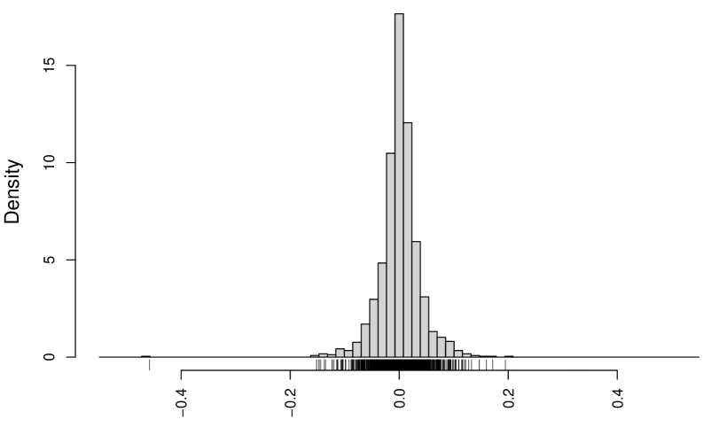
Refer to caption
(a) BTC-EUR
Refer to caption
(b) TRX-EUR
Figure 10: Histograms of the considered cryptocurrency daily returns.

5.2 Results

Motivated by the findings above, especially those related to shape, skewness and kurtosis of the empirical distributions, we fit our ALSMs to the considered cryptocurrency returns. For the sake of comparison, we also fit several parametric distributions defined on the whole real line. We take the competing models among those implemented in the gamlss package (Rigby & Stasinopoulos, 2005) for R. In detail, we consider the following distributions, given in alphabetic order using the nomenclature by Rigby et al. (2019): exponential Gaussian (exGAUS), generalized t𝑡t (GT), Gumbel (GU), Johnson’s SU (JSU), logistic (LO), NET (NET), normal (NO), normal family (NOF), power exponential (PE), reverse Gumbel (RG), sinh-arcsinh (SHASH), sinh-arcsinh original (SHASHo), skew normal type 1 (SN1), skew normal type 2 (SN2), skew power exponential type 1 (SEP1), skew power exponential type 2 (SEP2), skew power exponential type 3 (SEP3), skew power exponential type 4 (SEP4), skew Student t𝑡t (SST), skew t𝑡t type 1 (ST1), skew t𝑡t type 2 (ST2), skew t𝑡t type 4 (ST4), skew t𝑡t type 5 (ST5), and t𝑡t family (TF). Moreover, for the sake of completeness, and motivated by the results in Chu et al. (2015) and Chan et al. (2017), we also fit the generalyzed hyperbolic (GH) and some of its special cases which are not implemented in the gamlss package, namely hyperbolic (H), variance gamma (VG), and normal inverse Gaussian (NIG) distributions. These models are fitted via the fit.ghypuv() function of the ghyp package. This yields a total of 36 competing models. We estimate the parameters of all the models under consideration via the ML approach.

To compare models with the same number of parameters, in terms of goodness-of-fit, we use the log-likelihood (in addition to the criteria described below). We accomplish the comparison of models with differing number of parameters, as usual, via the Akaike information criterion (AIC; Akaike, 1974) and the Bayesian information criterion (BIC; Schwarz, 1978) that, in our formulation, need to be maximized because they are multiplied by 11-1. Moreover, we use the likelihood-ratio (LR) test to compare each Laplace-based model (alternative model) with the nested asymmetric Laplace distribution (null model). In particular, the LR test can be used to determine whether the alternative model is a significant improvement over the asymmetric Laplace distribution. The test statistic is

LR=2[l(μ^,β^,κ^)l(μ^,β^,κ^,𝜽^)],LR2delimited-[]𝑙^𝜇^𝛽^𝜅𝑙^𝜇^𝛽^𝜅^𝜽\text{LR}=-2\left[l(\widehat{\mu},\widehat{\beta},\widehat{\kappa})-l(\widehat{\mu},\widehat{\beta},\widehat{\kappa},\widehat{\bm{\theta}})\right],

where μ^^𝜇\widehat{\mu}, β^^𝛽\widehat{\beta}, κ^^𝜅\widehat{\kappa} and 𝜽^^𝜽\widehat{\bm{\theta}} are the ML estimates of μ𝜇\mu, β𝛽\beta, κ𝜅\kappa and 𝜽𝜽\bm{\theta}, respectively, and where l(μ^,β^,κ^)𝑙^𝜇^𝛽^𝜅l(\widehat{\mu},\widehat{\beta},\widehat{\kappa}) and l(μ^,β^,κ^,𝜽^)𝑙^𝜇^𝛽^𝜅^𝜽l(\widehat{\mu},\widehat{\beta},\widehat{\kappa},\widehat{\bm{\theta}}) are the maximized log-likelihood values under the null and alternative models, respectively. Under the null hypothesis of no improvement, using Wilks’ theorem, LR can be approximated by a χ2superscript𝜒2\chi^{2} random variable with number of degrees of freedom given by the difference in the number of estimated parameters between the alternative and the null model, and this allows us to compute a p𝑝p-value.

Tables 23 present the model comparison separately for each cryptocurrency. To easy the reader in comparing the performance of the considered parametric models, the tables also give rankings induced by AIC, BIC, and LR tests (limited to the AL-based models).

Model ##\# par Log-lik AIC Rank BIC Rank LR p𝑝p-value Rank
AL 3 3020.921 6035.842 18 6019.861 15
TP-AL 5 3027.713 6045.426 7 6018.790 17 0.001 6
SE-AL 4 3026.311 6044.621 8 6023.313 7 0.001 5
UG-AL 4 3027.701 6047.402 4 6026.094 5 0.000 3
IG-AL 4 3027.388 6046.776 5 6025.467 6 0.000 4
PF-AL 4 3028.167 6048.334 2 6027.026 3 0.000 2
P-AL 4 3025.807 6043.614 13 6022.306 12 0.002 7
U-AL 4 3047.685 6087.370 1 6066.062 1 0.000 1
exGAUS 3 2818.553 5631.105 31 5615.124 32
GH 5 3025.958 6041.917 16 6015.281 18
GT 4 3027.728 6047.455 3 6026.147 4
GU 2 2593.517 5183.034 35 5172.380 35
H 4 3020.920 6033.841 20 6012.532 20
JSU 4 3018.886 6029.773 21 6008.464 21
LO 2 2962.209 5920.419 29 5909.765 29
NET 2 2988.639 5969.277 28 5947.969 28
NIG 4 3021.583 6035.167 19 6013.858 19
NO 2 2816.573 5629.146 32 5618.491 31
NOF 3 2816.573 5627.146 33 5611.164 33
PE 3 3026.119 6046.239 6 6030.257 2
RG 2 1909.950 3815.899 36 3805.245 36
SHASH 4 3025.711 6043.422 14 6022.113 13
SHASHo 4 3025.522 6043.044 15 6021.735 14
SN1 3 2816.573 5627.146 34 5611.164 34
SN2 3 2820.347 5634.693 30 5618.712 30
SEP1 4 3026.126 6044.253 11 6022.944 10
SEP2 4 3026.146 6044.292 10 6022.984 9
SEP3 4 3026.120 6044.241 12 6022.932 11
SEP4 4 3026.208 6044.416 9 6023.108 8
SST 4 3012.351 6016.702 27 5995.394 27
ST1 4 3012.427 6016.853 23 5995.545 23
ST2 4 3012.360 6016.719 26 5995.411 26
ST4 4 3012.363 6016.725 25 5995.417 25
ST5 4 3012.363 6016.726 24 5995.418 24
TF 3 3012.320 6018.641 22 6002.659 22
VG 4 3024.470 6040.940 17 6019.631 16
Table 2: BTC-EUR: number of parameters (##\# par), log-likelihood (Log-lik), AIC, and BIC for the competing models, along with rankings from these criteria. The p𝑝p-values from the LR tests for the asymmetric Laplace-based models are given along with rankings.
Model ##\# par Log-lik AIC Rank BIC Rank LR p𝑝p-value Rank
AL 3 2383.212 4760.423 20 4744.442 8
TP-AL 5 2388.481 4766.963 5 4740.327 18 0.005 5
SE-AL 4 2386.362 4764.723 11 4743.415 11 0.012 6
UG-AL 4 2387.646 4767.293 4 4745.984 5 0.003 3
IG-AL 4 2387.405 4766.810 6 4745.501 6 0.004 4
PF-AL 4 2388.365 4768.731 3 4747.422 4 0.001 2
P-AL 4 2385.815 4763.630 14 4742.322 13 0.022 7
U-AL 4 2409.962 4811.925 1 4790.617 1 0.000 1
exGAUS 3 2213.975 4421.950 30 4405.969 30
GH 5 2388.037 4766.073 7 4739.438 20
GT 4 2388.430 4768.861 2 4747.552 3
GU 2 1902.159 3800.318 35 3789.663 35
H 4 2383.211 4758.423 21 4737.114 22
JSU 4 2384.976 4761.952 18 4740.644 17
LO 2 2333.869 4663.738 29 4653.084 29
NET 2 2360.386 4712.772 28 4691.463 28
NIG 4 2386.959 4765.918 8 4744.610 7
NO 2 2202.754 4401.507 31 4390.853 31
NOF 3 2202.626 4399.253 34 4383.271 34
PE 3 2385.124 4764.247 12 4748.266 2
RG 2 1587.234 3170.468 36 3159.814 36
SHASH 4 2386.467 4764.933 10 4743.625 10
SHASHo 4 2386.468 4764.935 9 4743.627 9
SN1 3 2202.754 4399.507 33 4383.526 33
SN2 3 2203.538 4401.075 32 4385.094 32
SEP1 4 2385.688 4763.376 16 4742.068 15
SEP2 4 2385.830 4763.660 13 4742.351 12
SEP3 4 2385.763 4763.526 15 4742.218 14
SEP4 4 2385.322 4762.644 17 4741.335 16
SST 4 2380.241 4752.482 23 4731.174 23
ST1 4 2380.229 4752.458 24 4731.149 24
ST2 4 2380.222 4752.444 25 4731.136 25
ST4 4 2380.207 4752.414 27 4731.106 27
ST5 4 2380.218 4752.435 26 4731.127 26
TF 3 2380.206 4754.412 22 4738.430 21
VG 4 2384.530 4761.061 19 4739.752 19
Table 3: TRX-EUR: number of parameters (##\# par), log-likelihood (Log-lik), AIC, and BIC for the competing models, along with rankings from these criteria. The p𝑝p-values from the LR tests for the asymmetric Laplace-based models are given along with rankings.

For the BTC-EUR, Table 2 shows that both AIC and BIC indicate one of our models, the U-AL, as the best one. Furthermore, six out of the seven models we propose (all except P-AL) are in the first eight positions according to the AIC (GT and PE occupy the third and sixth positions, respectively) while five out of our seven models (all except P-AL and TP-AL) are in the first six positions according to the BIC (PE and GT occupy the second and fourth positions, respectively). These findings are further corroborated by the ranking induced by the LR-test, with the U-AL in the first position and the TP-AL and P-AL in the penultimate and last position, respectively. Moreover, at the 5% significance level, all our models represent a significant improvement over the asymmetric Laplace.

For the TRX-EUR (refer to Table 3) we observe similar results. The U-AL is still the best model for AIC, BIC and LR test. Moreover, based on the p𝑝p-values from the LR test, all our models still represent a significant improvement over the asymmetric Laplace at the 5% significance level.

A final interesting aspect to be noted is that, regardless of the considered cryptocurrency, the Gumbel-based models (RG and GU) are the worst models according to AIC and BIC.

6 Conclusions and future works

In this paper we further corroborate some recent findings about the cryptocurrency return distribution; in particular, we confirm it can be highly-peaked, skewed, and heavy-tailed, with a large excess kurtosis. To account for all these peculiarities, in a modeling perspective, we propose the asymmetric Laplace scale mixture (ALSM) family of distributions and, for illustrative purposes, we consider seven different members of this family. Advantageously with respect to the nested asymmetric Laplace distribution, the members of our family allow for a wider range of skewness values and for a larger excess kurtosis. These improvements allows the ALSM to be a convenient model for the distribution of cryptocurrency returns.

However, the novelty of the paper is not limited to the five illustrated models and the usefulness of our family is not restricted to cryptocurrencies. Indeed, other members of the family may be easily defined and other financial contexts, like those outlined in Kotz et al. (2012, Chapter 8), may benefit from the use of ALSMs.

References

  • Abramowitz & Stegun (1965) Abramowitz, M., & Stegun, I. A. (1965). Handbook of Mathematical Functions: With Formulas, Graphs, and Mathematical Tables volume 55 of Applied Mathematics Series. New York: Dover Publications.
  • Ahsanullah & Kabir (1974) Ahsanullah, M., & Kabir, A. B. M. L. (1974). A characterization of the power function distribution. The Canadian Journal of Statistics, 2, 95–98.
  • Akaike (1974) Akaike, H. (1974). A new look at the statistical model identification. IEEE Transactions on Automatic Control, 19, 716–723.
  • Askey & Daalhuis (2010) Askey, R. A., & Daalhuis, A. B. O. (2010). Generalized hypergeometric functions and Meijer G𝐺{G}-function.
  • Bagnato & Punzo (2013) Bagnato, L., & Punzo, A. (2013). Finite mixtures of unimodal beta and gamma densities and the k𝑘k-bumps algorithm. Computational Statistics, 28, 1571–1597.
  • Bariviera et al. (2017) Bariviera, A. F., Basgall, M. J., Hasperué, W., & Naiouf, M. (2017). Some stylized facts of the Bitcoin market. Physica A: Statistical Mechanics and its Applications, 484, 82–90.
  • Chan et al. (2017) Chan, S., Chu, J., Nadarajah, S., & Osterrieder, J. (2017). A statistical analysis of cryptocurrencies. Journal of Risk and Financial Management, 10, 1–24.
  • Chen (2000) Chen, S. X. (2000). Probability density function estimation using gamma kernels. Annals of the Institute of Statistical Mathematics, 52, 471–480.
  • Chu et al. (2015) Chu, J., Nadarajah, S., & Chan, S. (2015). Statistical analysis of the exchange rate of bitcoin. PLOS One, 10, e0133678.
  • Coffey & Muller (2000) Coffey, C. S., & Muller, K. E. (2000). Properties of doubly-truncated gamma variables. Communications in Statistics-Theory and Methods, 29, 851–857.
  • Davies & Gather (1993) Davies, L., & Gather, U. (1993). The identification of multiple outliers. Journal of the American Statistical Association, 88, 782–792.
  • Dempster et al. (1977) Dempster, A. P., Laird, N. M., & Rubin, D. B. (1977). Maximum likelihood from incomplete data via the EM algorithm. Journal of the Royal Statistical Society: Series B (Statistical Methodology), 39, 1–38.
  • Dwork (1990) Dwork, B. (1990). Generalized hypergeometric functions. Clarendon Press.
  • Hennig (2002) Hennig, C. (2002). Fixed point clusters for linear regression: computation and comparison. Journal of Classification, 19, 249–276.
  • Johnson & Kotz (1970a) Johnson, N. L., & Kotz, S. (1970a). Continuous Univariate Distributions volume 2. New York: John Wiley & Sons.
  • Johnson & Kotz (1970b) Johnson, N. L., & Kotz, S. (1970b). Continuous Univariate Distributions volume 1. New York: John Wiley & Sons.
  • Kotz et al. (2001) Kotz, S., Kozubowski, T., & Podgórski, K. (2001). The Laplace distribution and generalizations: a revisit with applications to communications, economics, engineering, and finance. 183. Springer Science & Business Media.
  • Kotz et al. (2012) Kotz, S., Kozubowski, T. J., & Podgorski, K. (2012). The Laplace Distribution and Generalizations: A Revisit with Applications to Communications, Economics, Engineering, and Finance. SpringerLink : Bücher. Birkhäuser Boston.
  • Kozubowski & Podgorski (2000) Kozubowski, T. J., & Podgorski, K. (2000). Asymmetric laplace distributions. Mathematical Scientist, 25, 37–46.
  • Liu & Rubin (1994) Liu, C., & Rubin, D. B. (1994). The ECME algorithm: a simple extension of EM and ECM with faster monotone convergence. Biometrika, 81, 633–648.
  • Mazza & Punzo (2019) Mazza, A., & Punzo, A. (2019). Modeling household income with contaminated unimodal distributions. In A. Petrucci, F. Racioppi, & R. Verde (Eds.), New Statistical Developments in Data Science (pp. 373–391). Cham, Switzerland: Springer volume 88 of Springer Proceedings in Mathematics & Statistics.
  • McLachlan & Krishnan (2007) McLachlan, G., & Krishnan, T. (2007). The EM algorithm and extensions volume 382 of Wiley Series in Probability and Statistics. (2nd ed.). New York: John Wiley & Sons.
  • McNeil et al. (2005) McNeil, A., Frey, R., & Embrechts, P. (2005). Quantitative Risk Management: Concepts, Techniques and Tools. Princeton Series in Finance. Princeton University Press.
  • Melnykov & Zhu (2018) Melnykov, V., & Zhu, X. (2018). On model-based clustering of skewed matrix data. Journal of Multivariate Analysis, 167, 181–194.
  • Melnykov & Zhu (2019) Melnykov, V., & Zhu, X. (2019). Studying crime trends in the USA over the years 2000–2012. Advances in Data Analysis and Classification, 13, 325–341.
  • Meng & Rubin (1993) Meng, X.-L., & Rubin, D. B. (1993). Maximum likelihood estimation via the ECM algorithm: A general framework. Biometrika, 80, 267–278.
  • Misra (1940) Misra, R. D. (1940). On the stability of crystal lattices. II. Mathematical Proceedings of the Cambridge Philosophical Society, 36, 173–182.
  • Morris et al. (2019) Morris, K., Punzo, A., McNicholas, P. D., & Browne, R. P. (2019). Asymmetric clusters and outliers: Mixtures of multivariate contaminated shifted asymmetric laplace distributions. Computational Statistics & Data Analysis, 132, 145–166.
  • Osterrieder (2017) Osterrieder, J. (2017). The statistics of bitcoin and cryptocurrencies. In Proceedings of the 2017 International Conference on Economics, Finance and Statistics (ICEFS 2017). Atlantis Press volume 26 of Advances in Economics, Business and Management Research.
  • Phillip et al. (2018) Phillip, A., Chan, J. S. K., & Peiris, S. (2018). A new look at cryptocurrencies. Economics Letters, 163, 6–9.
  • Punzo (2019) Punzo, A. (2019). A new look at the inverse Gaussian distribution with applications to insurance and economic data. Journal of Applied Statistics, 46, 1260–1287.
  • Punzo & Bagnato (2021a) Punzo, A., & Bagnato, L. (2021a). Modeling the cryptocurrency return distribution via Laplace scale mixtures. Physica A: Statistical Mechanics and its Applications, 563. doi:10.1016/j.physa.2020.125354.
  • Punzo & Bagnato (2021b) Punzo, A., & Bagnato, L. (2021b). The multivariate tail-inflated normal distribution and its application in finance. Journal of Statistical Computation and Simulation, 91, 1–36.
  • Punzo et al. (2018) Punzo, A., Bagnato, L., & Maruotti, A. (2018). Compound unimodal distributions for insurance losses. Insurance: Mathematics and Economics, 81, 95–107.
  • Punzo & McNicholas (2016) Punzo, A., & McNicholas, P. D. (2016). Parsimonious mixtures of multivariate contaminated normal distributions. Biometrical Journal, 58, 1506–1537.
  • Punzo & Tortora (2021) Punzo, A., & Tortora, C. (2021). Multiple scaled contaminated normal distribution and its application in clustering. Statistical Modelling, 21, 332–358.
  • R Core Team (2018) R Core Team (2018). R: A Language and Environment for Statistical Computing. R Foundation for Statistical Computing Vienna, Austria. URL: https://www.R-project.org/.
  • Rigby & Stasinopoulos (2005) Rigby, R. A., & Stasinopoulos, D. M. (2005). Generalized additive models for location, scale and shape. Journal of the Royal Statistical Society: Series C (Applied Statistics), 54, 507–554.
  • Rigby et al. (2019) Rigby, R. A., Stasinopoulos, M. D., Heller, G. Z., & De Bastiani, F. (2019). Distributions for Modeling Location, Scale, and Shape: Using GAMLSS in R. Chapman & Hall/CRC The R Series. CRC Press. URL: https://books.google.it/books?id=Tu-yDwAAQBAJ.
  • Rytgaard (1990) Rytgaard, M. (1990). Estimation in the pareto distribution. ASTIN Bulletin: The Journal of the IAA, 20, 201–216.
  • Schwarz (1978) Schwarz, G. (1978). Estimating the dimension of a model. The Annals of Statistics, 6, 461–464.
  • Shevchenko (2010) Shevchenko, P. V. (2010). Calculation of aggregate loss distributions. The Journal of Operational Risk, 5, 3–40.
  • Szczygielski et al. (2020) Szczygielski, J. J., Karathanasopoulos, A., & Zaremba, A. (2020). One shape fits all? A comprehensive examination of cryptocurrency return distributions. Applied Economics Letters, 27, 1567–1573.
  • Takaishi (2018) Takaishi, T. (2018). Statistical properties and multifractality of Bitcoin. Physica A: Statistical Mechanics and its Applications, 506, 507–519.
  • Templ et al. (2019) Templ, M., Gussenbauer, J., & Filzmoser, P. (2019). Evaluation of robust outlier detection methods for zero-inflated complex data. Journal of Applied Statistics, 47, 1144–1167.
  • Tomarchio & Punzo (2020) Tomarchio, S. D., & Punzo, A. (2020). Dichotomous unimodal compound models: Application to the distribution of insurance losses. Journal of Applied Statistics, 47, 2328–2353.
  • Watson (1995) Watson, G. N. (1995). A treatise on the theory of Bessel functions. Cambridge university press.
  • Yap & Sim (2011) Yap, B. W., & Sim, C. H. (2011). Comparisons of various types of normality tests. Journal of Statistical Computation and Simulation, 81, 2141–2155.
  • Zhang et al. (2018) Zhang, W., Wang, P., Li, X., & Shen, D. (2018). Some stylized facts of the cryptocurrency market. Applied Economics, 50, 5950–5965.

Appendix A Gamma asymmetric Laplace distribution

Let

h(w;θ)=(θ2)θ2eθ2wwθ21Γ(θ2),w>0,formulae-sequence𝑤𝜃superscript𝜃2𝜃2superscript𝑒𝜃2𝑤superscript𝑤𝜃21Γ𝜃2𝑤0h\left(w;\theta\right)=\displaystyle\frac{\left(\frac{\theta}{2}\right)^{\frac{\theta}{2}}e^{-\frac{\theta}{2}w}w^{\frac{\theta}{2}-1}}{\Gamma\left(\frac{\theta}{2}\right)},\quad w>0, (89)

with θ>0𝜃0\theta>0, be the pdf of the gamma distribution with shape and rate equal to θ/2𝜃2\theta/2. In symbols, W𝒢(θ/2,θ/2)similar-to𝑊𝒢𝜃2𝜃2W\sim\mathcal{G}\left(\theta/2,\theta/2\right). When the pdf in (89) is considered as mixing density in model (6), the pdf of the ALSM becomes

fALSM(x;μ,β,κ,θ)=1βκ1+κ2{[1+2κβθ(xμ)]θ21for xμ,[1+2βκθ(μx)]θ21for x<μ.subscript𝑓ALSM𝑥𝜇𝛽𝜅𝜃1𝛽𝜅1superscript𝜅2casessuperscriptdelimited-[]12𝜅𝛽𝜃𝑥𝜇𝜃21for xμ,superscriptdelimited-[]12𝛽𝜅𝜃𝜇𝑥𝜃21for x<μ.f_{\text{ALSM}}\left(x;\mu,\beta,\kappa,\theta\right)=\frac{1}{\beta}\frac{\kappa}{1+\kappa^{2}}\begin{cases}\left[1+\frac{2\kappa}{\beta\theta}\left(x-\mu\right)\right]^{-\frac{\theta}{2}-1}&\text{for $x\geq\mu$,}\\[8.53581pt] \left[1+\frac{2}{\beta\kappa\theta}\left(\mu-x\right)\right]^{-\frac{\theta}{2}-1}&\text{for $x<\mu$.}\end{cases} (90)

Although the pdf in (90) is a simple reparameterization of the pdf of the UG-AL model given in (33), for the sake of clarity/confusion we prefer referring to the resulting model as gamma asymmetric Laplace (G-AL). Model (90) reduces to 𝒜(μ,β,κ)𝒜𝜇𝛽𝜅\mathcal{AL}\left(\mu,\beta,\kappa\right) when θ𝜃\theta\rightarrow\infty.

When W𝒢(θ/2,θ/2)similar-to𝑊𝒢𝜃2𝜃2W\sim\mathcal{G}\left(\theta/2,\theta/2\right), the r𝑟rth raw moment of 1/W1𝑊1/W is

E(1Wr)E1superscript𝑊𝑟\displaystyle\text{E}\left(\frac{1}{W^{r}}\right) =θrΓ(θ2r)2rΓ(θ2),absentsuperscript𝜃𝑟Γ𝜃2𝑟superscript2𝑟Γ𝜃2\displaystyle=\frac{\theta^{r}\Gamma\left(\frac{\theta}{2}-r\right)}{2^{r}\Gamma\left(\frac{\theta}{2}\right)},
=θrj=1r(θ2j)absentsuperscript𝜃𝑟superscriptsubscriptproduct𝑗1𝑟𝜃2𝑗\displaystyle=\frac{\theta^{r}}{\displaystyle\prod_{j=1}^{r}\left(\theta-2j\right)} (91)

which exists when θ>2r𝜃2𝑟\theta>2r. By substituting in (12)–(15) the first four raw moments in (91), mean, variance, skewness and kurtosis of the G-AL distribution become

E(X)=μ+β(1κκ)θθ2,E𝑋𝜇𝛽1𝜅𝜅𝜃𝜃2\text{E}\left(X\right)=\mu+\beta\left(\frac{1}{\kappa}-\kappa\right)\frac{\theta}{\theta-2}, (92)

which exists if θ>2𝜃2\theta>2,

Var(X)=β2θ2(θκ4+θ4κ2)(θ4)(θ2)2κ2Var𝑋superscript𝛽2superscript𝜃2𝜃superscript𝜅4𝜃4superscript𝜅2𝜃4superscript𝜃22superscript𝜅2\text{Var}\left(X\right)=\frac{\beta^{2}\theta^{2}\left(\theta\kappa^{4}+\theta-4\kappa^{2}\right)}{(\theta-4)(\theta-2)^{2}\kappa^{2}} (93)

which exists if θ>4𝜃4\theta>4,

Skew(X)=2θ4(θ+2)(κ21)[θκ4+(θ6)κ2+θ](θ6)(θκ4+θ4κ2)3/2,Skew𝑋2𝜃4𝜃2superscript𝜅21delimited-[]𝜃superscript𝜅4𝜃6superscript𝜅2𝜃𝜃6superscript𝜃superscript𝜅4𝜃4superscript𝜅232\text{Skew}\left(X\right)=-\frac{2\sqrt{\theta-4}(\theta+2)\left(\kappa^{2}-1\right)\left[\theta\kappa^{4}+(\theta-6)\kappa^{2}+\theta\right]}{(\theta-6)\left(\theta\kappa^{4}+\theta-4\kappa^{2}\right)^{3/2}}, (94)

which exists if θ>6𝜃6\theta>6, and

Kurt(X)=Kurt𝑋absent\displaystyle\text{Kurt}\left(X\right)= 1(θ8)(θ6)(θκ4+θ4κ2)2[θ4(9κ8+6κ4+9)6θ3(5κ8+12κ6+6κ4+12κ2+5)+\displaystyle\frac{1}{(\theta-8)(\theta-6)\left(\theta\kappa^{4}+\theta-4\kappa^{2}\right)^{2}}\bigg{[}\theta^{4}\left(9\kappa^{8}+6\kappa^{4}+9\right)-6\theta^{3}\left(5\kappa^{8}+12\kappa^{6}+6\kappa^{4}+12\kappa^{2}+5\right)+
+48θ2κ2(5κ4+8κ2+5)96θ(κ8+12κ4+1)+768(κ6κ4+κ2)],\displaystyle+48\theta^{2}\kappa^{2}\left(5\kappa^{4}+8\kappa^{2}+5\right)-96\theta\left(\kappa^{8}+12\kappa^{4}+1\right)+768\left(\kappa^{6}-\kappa^{4}+\kappa^{2}\right)\bigg{]}, (95)

which exists if θ>8𝜃8\theta>8.

Figure 11 shows examples of behaviors of Skew(X)Skew𝑋\text{Skew}\left(X\right) and Kurt(X)Kurt𝑋\text{Kurt}\left(X\right), as functions of κ𝜅\kappa, at various levels of θ𝜃\theta.

Refer to caption
(a) Skewness
Refer to caption
(b) Kurtosis
Figure 11: Examples of behavior of Skew(X)Skew𝑋\text{Skew}\left(X\right) (on the left) and Kurt(X)Kurt𝑋\text{Kurt}\left(X\right) (on the right), as functions of κ𝜅\kappa, at various levels of θ𝜃\theta for the G-AL distribution.

From Figure 11(a) we realize that: 1) large values of θ𝜃\theta tend to produce the plot of Skew(X)Skew𝑋\text{Skew}\left(X\right) we obtained for 𝒜(μ,β,κ)𝒜𝜇𝛽𝜅\mathcal{AL}\left(\mu,\beta,\kappa\right) (refer to Figure 1); and 2) as θ𝜃\theta decreases (to a minimum value of 6), the range of possible values of Skew(X)Skew𝑋\text{Skew}\left(X\right) increases. Moreover, to “significantly” modify the behavior of Skew(X)Skew𝑋\text{Skew}\left(X\right) with respect to the 𝒜(μ,β,κ)𝒜𝜇𝛽𝜅\mathcal{AL}\left(\mu,\beta,\kappa\right) case, we need low values of θ𝜃\theta (in the examples, θ=8𝜃8\theta=8 and θ=7𝜃7\theta=7). Similarly, from Figure 11(b) we realize that: 1) large values of θ𝜃\theta tend to produce the plot of Kurt(X)Kurt𝑋\text{Kurt}\left(X\right) we obtained for 𝒜(μ,β,κ)𝒜𝜇𝛽𝜅\mathcal{AL}\left(\mu,\beta,\kappa\right) (refer to Figure 1); and 2) κ𝜅\kappa kept fixed, the lower the value θ𝜃\theta (with a minimum of 8), the higher the kurtosis. This means that the curve obtained for θ𝜃\theta\rightarrow\infty acts as a lower bound. Also in this case, to “significantly” modify the behavior of Kurt(X)Kurt𝑋\text{Kurt}\left(X\right) with respect to the 𝒜(μ,β,κ)𝒜𝜇𝛽𝜅\mathcal{AL}\left(\mu,\beta,\kappa\right) case, we need low values of θ𝜃\theta (in the examples, θ=40𝜃40\theta=40 and θ=20𝜃20\theta=20).

Appendix B E- and M-steps for the G-AL distribution

For the G-AL distribution we have

l2c(θ)=nθ2log(θ2)nlog[Γ(θ2)]+(θ21)i=1nlogwiθ2i=1nwi.subscript𝑙2𝑐𝜃𝑛𝜃2𝜃2𝑛Γ𝜃2𝜃21superscriptsubscript𝑖1𝑛subscript𝑤𝑖𝜃2superscriptsubscript𝑖1𝑛subscript𝑤𝑖l_{2c}\left(\theta\right)=\frac{n\theta}{2}\log\left(\frac{\theta}{2}\right)-n\log\left[\Gamma\left(\frac{\theta}{2}\right)\right]+\left(\frac{\theta}{2}-1\right)\sum_{i=1}^{n}\log w_{i}-\frac{\theta}{2}\sum_{i=1}^{n}w_{i}. (96)

B.1 E-step

As for the E-step,

f(wi|xi;μ,β,κ,θ)𝑓conditionalsubscript𝑤𝑖subscript𝑥𝑖𝜇𝛽𝜅𝜃\displaystyle f\left(w_{i}|x_{i};\mu,\beta,\kappa,\theta\right) f(wi,xi;μ,β,κ,θ)proportional-toabsent𝑓subscript𝑤𝑖subscript𝑥𝑖𝜇𝛽𝜅𝜃\displaystyle\propto f\left(w_{i},x_{i};\mu,\beta,\kappa,\theta\right)
fG(wi;θ2+1,δ(xi;μ,β,κ)+θ2).proportional-toabsentsubscript𝑓Gsubscript𝑤𝑖𝜃21𝛿subscript𝑥𝑖𝜇𝛽𝜅𝜃2\displaystyle\propto f_{\text{G}}\left(w_{i};\frac{\theta}{2}+1,\delta\left(x_{i};\mu,\beta,\kappa\right)+\frac{\theta}{2}\right). (97)

This means that Wi|Xi=xiconditionalsubscript𝑊𝑖subscript𝑋𝑖subscript𝑥𝑖W_{i}|X_{i}=x_{i} has a gamma distribution with shape θ/2+1𝜃21\theta/2+1 and rate δ(xi;μ,β,κ)+θ/2𝛿subscript𝑥𝑖𝜇𝛽𝜅𝜃2\delta\left(x_{i};\mu,\beta,\kappa\right)+\theta/2, whose pdf is given in (97); in symbols

Wi|Xi=xi𝒢(θ2+1,δ(xi;μ,β,κ)+θ2).conditionalsubscript𝑊𝑖subscript𝑋𝑖subscript𝑥𝑖similar-to𝒢𝜃21𝛿subscript𝑥𝑖𝜇𝛽𝜅𝜃2W_{i}|X_{i}=x_{i}\sim\mathcal{G}\left(\frac{\theta}{2}+1,\delta\left(x_{i};\mu,\beta,\kappa\right)+\frac{\theta}{2}\right).

The functions g(Wi)𝑔subscript𝑊𝑖g(W_{i}) arising from (68) and (96) are g1(w)=wsubscript𝑔1𝑤𝑤g_{1}\left(w\right)=w and g2(w)=log(w)subscript𝑔2𝑤𝑤g_{2}\left(w\right)=\log\left(w\right). Thanks to (97) we obtain

E˙(Wi|Xi=xi)˙Econditionalsubscript𝑊𝑖subscript𝑋𝑖subscript𝑥𝑖\displaystyle\dot{\mbox{E}}\left(W_{i}|X_{i}=x_{i}\right) =θ˙2+1δ(xi;μ˙,β˙,κ˙)+θ˙2absent˙𝜃21𝛿subscript𝑥𝑖˙𝜇˙𝛽˙𝜅˙𝜃2\displaystyle=\frac{\frac{\dot{\theta}}{2}+1}{\delta\left(x_{i};\dot{\mu},\dot{\beta},\dot{\kappa}\right)+\frac{\dot{\theta}}{2}}
w˙iabsentsubscript˙𝑤𝑖\displaystyle\eqqcolon\dot{w}_{i}

and

E˙(logWi|Xi=xi)˙Econditionalsubscript𝑊𝑖subscript𝑋𝑖subscript𝑥𝑖\displaystyle\dot{\mbox{E}}\left(\log W_{i}|X_{i}=x_{i}\right) =ψ(θ˙2+1)log[δ(xi;μ˙,β˙,κ˙)+θ˙2]absent𝜓˙𝜃21𝛿subscript𝑥𝑖˙𝜇˙𝛽˙𝜅˙𝜃2\displaystyle=\psi\left(\frac{\dot{\theta}}{2}+1\right)-\log\left[\delta\left(x_{i};\dot{\mu},\dot{\beta},\dot{\kappa}\right)+\frac{\dot{\theta}}{2}\right]
log˙wi.absent˙subscript𝑤𝑖\displaystyle\eqqcolon\dot{\log}\>w_{i}.

B.2 M-step

For the G-AL distribution, a closed-form update for θ𝜃\theta does not exist. The function to maximize is

Q2(θ|μ˙,β˙,κ˙,θ˙)=θ2(i=1nlog˙wii=1nw˙i)nθ2log(θ2)nlog[Γ(θ2)],subscript𝑄2conditional𝜃˙𝜇˙𝛽˙𝜅˙𝜃𝜃2superscriptsubscript𝑖1𝑛˙subscript𝑤𝑖superscriptsubscript𝑖1𝑛subscript˙𝑤𝑖𝑛𝜃2𝜃2𝑛Γ𝜃2Q_{2}\left(\theta|\dot{\mu},\dot{\beta},\dot{\kappa},\dot{\theta}\right)=\frac{\theta}{2}\left(\sum_{i=1}^{n}\dot{\log}\>w_{i}-\sum_{i=1}^{n}\dot{w}_{i}\right)-\frac{n\theta}{2}\log\left(\frac{\theta}{2}\right)-n\log\left[\Gamma\left(\frac{\theta}{2}\right)\right], (98)

whose derivative, with respect to θ𝜃\theta, is

Q2(θ|μ˙,β˙,κ˙,θ˙)θ=12(i=1nlog˙wii=1nw˙i)n2[ψ(θ2)+log(θ2)+1].subscript𝑄2conditional𝜃˙𝜇˙𝛽˙𝜅˙𝜃𝜃12superscriptsubscript𝑖1𝑛˙subscript𝑤𝑖superscriptsubscript𝑖1𝑛subscript˙𝑤𝑖𝑛2delimited-[]𝜓𝜃2𝜃21\frac{\partial Q_{2}\left(\theta|\dot{\mu},\dot{\beta},\dot{\kappa},\dot{\theta}\right)}{\partial\theta}=\frac{1}{2}\left(\sum_{i=1}^{n}\dot{\log}\>w_{i}-\sum_{i=1}^{n}\dot{w}_{i}\right)-\frac{n}{2}\left[\psi\left(\frac{\theta}{2}\right)+\log\left(\frac{\theta}{2}\right)+1\right]. (99)

The update for θ𝜃\theta can be obtained numerically either by maximizing (98) over θ𝜃\theta or by finding the root (over θ𝜃\theta) of the equation obtained equating (99) to zero.

Appendix C Method of moments

In the method of moments (MM) applied to the estimation of the parameters of the ALSM distribution, we relate the (unknown) population moments in (12)–(15) to their sample counterparts

x¯=1ni=1nxi,s2=1n1i=1n(xix¯)2,formulae-sequence¯𝑥1𝑛superscriptsubscript𝑖1𝑛subscript𝑥𝑖superscript𝑠21𝑛1superscriptsubscript𝑖1𝑛superscriptsubscript𝑥𝑖¯𝑥2\overline{x}=\frac{1}{n}\sum_{i=1}^{n}x_{i},\quad s^{2}=\frac{1}{n-1}\sum_{i=1}^{n}\left(x_{i}-\overline{x}\right)^{2},
Skew^(X)=1ns3i=1n(xix¯)3,andKurt^(X)=1ns4i=1n(xix¯)4.formulae-sequence^Skew𝑋1𝑛superscript𝑠3superscriptsubscript𝑖1𝑛superscriptsubscript𝑥𝑖¯𝑥3and^Kurt𝑋1𝑛superscript𝑠4superscriptsubscript𝑖1𝑛superscriptsubscript𝑥𝑖¯𝑥4\widehat{\text{Skew}}(X)=\frac{1}{ns^{3}}\sum_{i=1}^{n}\left(x_{i}-\overline{x}\right)^{3},\quad\text{and}\quad\widehat{\text{Kurt}}(X)=\frac{1}{ns^{4}}\sum_{i=1}^{n}\left(x_{i}-\overline{x}\right)^{4}.

Apart from the TP-AL distribution, where 𝜽𝜽\bm{\theta} is bidimensional, for all the other models it is unidimensional. For these models, with the aim to find the MM estimates of μ𝜇\mu, β𝛽\beta, κ𝜅\kappa, and θ𝜃\theta, we have to solve a system of four equations. In doing that, it is important to remember that the four equations involve a different number of parameters (refer to Section 2.4). So, it is convenient to first find the estimates κ^^𝜅\widehat{\kappa} and θ^^𝜃\widehat{\theta} by solving the system of the two equations Skew(X)=Skew^(X)Skew𝑋^Skew𝑋\text{Skew}(X)=\widehat{\text{Skew}}(X) and Kurt(X)=Kurt^(X)Kurt𝑋^Kurt𝑋\text{Kurt}(X)=\widehat{\text{Kurt}}(X). To search for the roots of the system of the two nonlinear equations, we use the nleqslv() function included in the nleqslv package. Moreover, to ensure the existence of the moments we have to impose (if necessary) suitable constraints for θ𝜃\theta (refer to Section 3). Then, based on (13), we solve the equation Var(X)=s2Var𝑋superscript𝑠2\text{Var}(X)=s^{2} as a function of β𝛽\beta with κ𝜅\kappa and θ𝜃\theta replaced by κ^^𝜅\widehat{\kappa} and θ^^𝜃\widehat{\theta}, respectively; this leads to

β^=s2κ^2(1+κ^2)2(1+κ^6)E^(1W2)(1κ^4)(1κ^2)E^(1W)2,^𝛽superscript𝑠2superscript^𝜅21superscript^𝜅221superscript^𝜅6^E1superscript𝑊21superscript^𝜅41superscript^𝜅2^Esuperscript1𝑊2\widehat{\beta}=\sqrt{\frac{s^{2}\widehat{\kappa}^{2}\left(1+\widehat{\kappa}^{2}\right)}{2\left(1+\widehat{\kappa}^{6}\right)\widehat{\text{E}}\left(\frac{1}{W^{2}}\right)-\left(1-\widehat{\kappa}^{4}\right)\left(1-\widehat{\kappa}^{2}\right)\widehat{\text{E}}\left(\frac{1}{W}\right)^{2}}}, (100)

where the quantities E^(1Wr)^E1superscript𝑊𝑟\widehat{\text{E}}\left(\frac{1}{W^{r}}\right), with r=1,2𝑟12r=1,2, are estimates of E(1Wr)E1superscript𝑊𝑟\text{E}\left(\frac{1}{W^{r}}\right) obtained using θ^^𝜃\widehat{\theta}. Finally, based on (12), we solve the equation E(X)=x¯E𝑋¯𝑥\text{E}(X)=\overline{x} as a function of μ𝜇\mu with β𝛽\beta, κ𝜅\kappa and θ𝜃\theta replaced by β^^𝛽\widehat{\beta}, κ^^𝜅\widehat{\kappa} and θ^^𝜃\widehat{\theta}, respectively; this leads to

μ^=x¯β^(1κ^κ^)E^(1W).^𝜇¯𝑥^𝛽1^𝜅^𝜅^E1𝑊\widehat{\mu}=\overline{x}-\widehat{\beta}\left(\frac{1}{\widehat{\kappa}}-\widehat{\kappa}\right)\widehat{\text{E}}\left(\frac{1}{W}\right). (101)

Appendix D M-Step details

With the aim to maximize Q1(μ,β,κ|μ˙,β˙,κ˙,𝜽˙)subscript𝑄1𝜇𝛽conditional𝜅˙𝜇˙𝛽˙𝜅˙𝜽Q_{1}\left(\mu,\beta,\kappa|\dot{\mu},\dot{\beta},\dot{\kappa},\dot{\bm{\theta}}\right) we consider the following two cases:

Case 1,

only μ𝜇\mu is known;

Case 2,

all parameters are unknown.

D.1 Case 1

Maximizing Q1(μ,β,κ|μ˙,β˙,κ˙,𝜽˙)subscript𝑄1𝜇𝛽conditional𝜅˙𝜇˙𝛽˙𝜅˙𝜽Q_{1}\left(\mu,\beta,\kappa|\dot{\mu},\dot{\beta},\dot{\kappa},\dot{\bm{\theta}}\right) is the same as maximizing n1Q1(μ,β,κ|μ˙,β˙,κ˙,𝜽˙)superscript𝑛1subscript𝑄1𝜇𝛽conditional𝜅˙𝜇˙𝛽˙𝜅˙𝜽n^{-1}\>Q_{1}\left(\mu,\beta,\kappa|\dot{\mu},\dot{\beta},\dot{\kappa},\dot{\bm{\theta}}\right) which, when the value of μ𝜇\mu is known, reduces to

Q(β,κ)=logκlog(1+κ2)logβ1β(κ,1/k)𝒁¯(n),𝑄𝛽𝜅𝜅1superscript𝜅2𝛽1𝛽𝜅1𝑘superscript¯𝒁𝑛Q\left(\beta,\kappa\right)=\log\kappa-\log\left(1+\kappa^{2}\right)-\log\beta-\frac{1}{\beta}\left(\kappa,1/k\right)\bar{\bm{Z}}^{(n)}, (102)

where 𝒁¯(n)superscript¯𝒁𝑛\bar{\bm{Z}}^{(n)} is defined as

𝒁¯(n)=(Z¯1(n),Z¯2(n)),superscript¯𝒁𝑛superscriptsuperscriptsubscript¯𝑍1𝑛superscriptsubscript¯𝑍2𝑛\bar{\bm{Z}}^{(n)}=\left(\bar{Z}_{1}^{(n)},\bar{Z}_{2}^{(n)}\right)^{\prime}, (103)

with

Z¯1(n)=1ni=1nw˙i(xiμ)+andZ¯2(n)=1ni=1nw˙i(xiμ).formulae-sequencesuperscriptsubscript¯𝑍1𝑛1𝑛superscriptsubscript𝑖1𝑛subscript˙𝑤𝑖superscriptsubscript𝑥𝑖𝜇andsuperscriptsubscript¯𝑍2𝑛1𝑛superscriptsubscript𝑖1𝑛subscript˙𝑤𝑖superscriptsubscript𝑥𝑖𝜇\bar{Z}_{1}^{(n)}=\frac{1}{n}\sum_{i=1}^{n}\dot{w}_{i}\left(x_{i}-\mu\right)^{+}\quad\text{and}\quad\bar{Z}_{2}^{(n)}=\frac{1}{n}\sum_{i=1}^{n}\dot{w}_{i}\left(x_{i}-\mu\right)^{-}. (104)

The parameter μ𝜇\mu could be: i) μx(1)𝜇subscript𝑥1\mu\leq x_{(1)}, ii) μx(n)𝜇subscript𝑥𝑛\mu\geq x_{(n)}, or iii) x(1)<μ<x(n)subscript𝑥1𝜇subscript𝑥𝑛x_{(1)}<\mu<x_{(n)}. If i) holds, then all sample values are greater or equal to μ𝜇\mu; this means that

(xiμ)+=(xiμ)and(xiμ)=0for all i=1,,n.formulae-sequencesuperscriptsubscript𝑥𝑖𝜇subscript𝑥𝑖𝜇andsuperscriptsubscript𝑥𝑖𝜇0for all i=1,,n\left(x_{i}-\mu\right)^{+}=\left(x_{i}-\mu\right)\quad\text{and}\quad\left(x_{i}-\mu\right)^{-}=0\quad\text{for all $i=1,\ldots,n$}.

Thus,

𝒁¯(n)=(x¯w(n),0),superscript¯𝒁𝑛superscriptsubscriptsuperscript¯𝑥𝑛𝑤0\bar{\bm{Z}}^{(n)}=\left(\bar{x}^{(n)}_{w},0\right)^{\prime}, (105)

where

x¯w(n)=1ni=1nw˙i(xiμ).subscriptsuperscript¯𝑥𝑛𝑤1𝑛superscriptsubscript𝑖1𝑛subscript˙𝑤𝑖subscript𝑥𝑖𝜇\bar{x}^{(n)}_{w}=\frac{1}{n}\sum_{i=1}^{n}\dot{w}_{i}\left(x_{i}-\mu\right). (106)

Therefore, (102) takes the form

Q(β,κ)=logκlog(1+κ2)logβκβx¯w(n).𝑄𝛽𝜅𝜅1superscript𝜅2𝛽𝜅𝛽subscriptsuperscript¯𝑥𝑛𝑤Q\left(\beta,\kappa\right)=\log\kappa-\log\left(1+\kappa^{2}\right)-\log\beta-\frac{\kappa}{\beta}\bar{x}^{(n)}_{w}. (107)

Fix κ>0𝜅0\kappa>0 and differentiate (107) with respect to β𝛽\beta to obtain

Q(β,κ)β=1β+κβ2x¯w(n).𝑄𝛽𝜅𝛽1𝛽𝜅superscript𝛽2subscriptsuperscript¯𝑥𝑛𝑤\frac{\partial Q\left(\beta,\kappa\right)}{\partial\beta}=-\frac{1}{\beta}+\frac{\kappa}{\beta^{2}}\bar{x}^{(n)}_{w}. (108)

The derivative (108) is positive for β<β(κ)𝛽𝛽𝜅\beta<\beta(\kappa) and negative for β>β(κ)𝛽𝛽𝜅\beta>\beta(\kappa), where

β(κ)=κx¯w(n).𝛽𝜅𝜅subscriptsuperscript¯𝑥𝑛𝑤\beta(\kappa)=\kappa\>\bar{x}^{(n)}_{w}.

As a consequence, for any fixed κ>0𝜅0\kappa>0, (107) is maximized by β(κ)𝛽𝜅\beta(\kappa). Then, for all σ𝜎\sigma and κ𝜅\kappa, we have

Q(β,κ)Q(β(κ),κ)=log(1+κ2)logx¯w(n)1,𝑄𝛽𝜅𝑄𝛽𝜅𝜅1superscript𝜅2subscriptsuperscript¯𝑥𝑛𝑤1Q\left(\beta,\kappa\right)\leq Q\left(\beta(\kappa),\kappa\right)=-\log\left(1+\kappa^{2}\right)-\log\bar{x}^{(n)}_{w}-1, (109)

where Q(β(κ),κ)𝑄𝛽𝜅𝜅Q\left(\beta(\kappa),\kappa\right) is a function of κ𝜅\kappa only and it is decreasing on (0,)0(0,\infty), with the least upper bound being equal to

limk0Q(β(κ),κ)=logx¯w(n)1.subscript𝑘0𝑄𝛽𝜅𝜅subscriptsuperscript¯𝑥𝑛𝑤1\lim_{k\rightarrow 0}Q\left(\beta(\kappa),\kappa\right)=-\log\bar{x}^{(n)}_{w}-1.

Since these values are not admissible, formally the M-step solutions of κ𝜅\kappa and β𝛽\beta do not exist in this case. However, as κ0+𝜅superscript0\kappa\rightarrow 0^{+} and β(κ)0+𝛽𝜅superscript0\beta(\kappa)\rightarrow 0^{+}, the conditional 𝒜(μ,β/w,κ)𝒜𝜇𝛽𝑤𝜅\mathcal{AL}\left(\mu,\beta/w,\kappa\right) in (6) tends to 𝒮(μ,)(w)𝒮subscript𝜇𝑤\mathcal{SE}_{\left(\mu,\infty\right)}\left(w\right).

If we are in the case ii), then all sample values are lower or equal to μ𝜇\mu. This means that

(xiμ)+=0and(xiμ)=(μxi)for all i=1,,n.formulae-sequencesuperscriptsubscript𝑥𝑖𝜇0andsuperscriptsubscript𝑥𝑖𝜇𝜇subscript𝑥𝑖for all i=1,,n\left(x_{i}-\mu\right)^{+}=0\quad\text{and}\quad\left(x_{i}-\mu\right)^{-}=\left(\mu-x_{i}\right)\quad\text{for all $i=1,\ldots,n$}.

Thus,

𝒁¯(n)=(0,x¯w(n)).superscript¯𝒁𝑛superscript0subscriptsuperscript¯𝑥𝑛𝑤\bar{\bm{Z}}^{(n)}=\left(0,-\bar{x}^{(n)}_{w}\right)^{\prime}. (110)

Then, (102) takes the form

Q(β,κ)=logκlog(1+κ2)logβ+1βκx¯w(n).𝑄𝛽𝜅𝜅1superscript𝜅2𝛽1𝛽𝜅subscriptsuperscript¯𝑥𝑛𝑤Q\left(\beta,\kappa\right)=\log\kappa-\log\left(1+\kappa^{2}\right)-\log\beta+\frac{1}{\beta\kappa}\bar{x}^{(n)}_{w}. (111)

Fix κ>0𝜅0\kappa>0 and differentiate (111) with respect to β𝛽\beta to obtain

Q(β,κ)β=1β1β2κx¯w(n).𝑄𝛽𝜅𝛽1𝛽1superscript𝛽2𝜅subscriptsuperscript¯𝑥𝑛𝑤\frac{\partial Q\left(\beta,\kappa\right)}{\partial\beta}=-\frac{1}{\beta}-\frac{1}{\beta^{2}\kappa}\bar{x}^{(n)}_{w}. (112)

The derivative (112) is positive for β<β(κ)𝛽𝛽𝜅\beta<\beta(\kappa) and negative for β>β(κ)𝛽𝛽𝜅\beta>\beta(\kappa), where

β(κ)=x¯w(n)κ.𝛽𝜅subscriptsuperscript¯𝑥𝑛𝑤𝜅\beta(\kappa)=-\frac{\bar{x}^{(n)}_{w}}{\kappa}.

Therefore, for any fixed κ>0𝜅0\kappa>0, (111) is maximized by β(κ)𝛽𝜅\beta(\kappa). Hence, for all σ𝜎\sigma and κ𝜅\kappa, we have

Q(β,κ)Q(β(κ),κ)=log(κ21+κ2)log(x¯w(n))1,𝑄𝛽𝜅𝑄𝛽𝜅𝜅superscript𝜅21superscript𝜅2subscriptsuperscript¯𝑥𝑛𝑤1Q\left(\beta,\kappa\right)\leq Q\left(\beta(\kappa),\kappa\right)=-\log\left(\frac{\kappa^{2}}{1+\kappa^{2}}\right)-\log\left(-\bar{x}^{(n)}_{w}\right)-1, (113)

where Q(β(κ),κ)𝑄𝛽𝜅𝜅Q\left(\beta(\kappa),\kappa\right) is a function of κ𝜅\kappa only and it is increasing on (0,)0(0,\infty), with the limit being equal to

limkQ(β(κ),κ)=log(x¯w(n))1.subscript𝑘𝑄𝛽𝜅𝜅subscriptsuperscript¯𝑥𝑛𝑤1\lim_{k\rightarrow\infty}Q\left(\beta(\kappa),\kappa\right)=-\log\left(-\bar{x}^{(n)}_{w}\right)-1.

Since these values are not admissible, formally the M-step solutions of κ𝜅\kappa and β𝛽\beta do not exist in this case. However, as κ𝜅\kappa\rightarrow\infty and β(κ)0+𝛽𝜅superscript0\beta(\kappa)\rightarrow 0^{+} we have that the conditional 𝒜(μ,β/w,κ)𝒜𝜇𝛽𝑤𝜅\mathcal{AL}\left(\mu,\beta/w,\kappa\right) in (6) tends to a “reversed” shifted exponential distribution with pdf

fSE(x;w)={0for xμ,wew(μx)for x<μ.subscript𝑓SE𝑥𝑤cases0for xμ𝑤superscript𝑒𝑤𝜇𝑥for x<μf_{\text{SE}}\left(x;w\right)=\begin{cases}0&\text{for $x\geq\mu$},\\ we^{-w\left(\mu-x\right)}&\text{for $x<\mu$}.\end{cases} (114)

Under case iii), that is when x(1)<μ<x(n)subscript𝑥1𝜇subscript𝑥𝑛x_{(1)}<\mu<x_{(n)}, we can find the solutions for β𝛽\beta and κ𝜅\kappa through the following equations of derivatives of Q(β,κ)𝑄𝛽𝜅Q\left(\beta,\kappa\right):

Q(β,κ)β=1β+1β2(κ,1/k)𝒁¯(n)=0Q(β,κ)κ=1κ2κ1+κ21β(1,1/k2)𝒁¯(n)=0.𝑄𝛽𝜅𝛽1𝛽1superscript𝛽2𝜅1𝑘superscript¯𝒁𝑛0missing-subexpression𝑄𝛽𝜅𝜅1𝜅2𝜅1superscript𝜅21𝛽11superscript𝑘2superscript¯𝒁𝑛0missing-subexpression\begin{array}[]{ll}\frac{\partial Q\left(\beta,\kappa\right)}{\partial\beta}=-\frac{1}{\beta}+\frac{1}{\beta^{2}}\left(\kappa,1/k\right)\bar{\bm{Z}}^{(n)}=0\\ \frac{\partial Q\left(\beta,\kappa\right)}{\partial\kappa}=\frac{1}{\kappa}-\frac{2\kappa}{1+\kappa^{2}}\par-\frac{1}{\beta}\left(1,-1/k^{2}\right)\bar{\bm{Z}}^{(n)}=0.\end{array} (115)

These equations are equivalent to

(κ,1/k)𝒁¯(n)=β(κ2,1/k2)𝒁¯(n)=0,𝜅1𝑘superscript¯𝒁𝑛𝛽missing-subexpressionsuperscript𝜅21superscript𝑘2superscript¯𝒁𝑛0missing-subexpression\begin{array}[]{ll}\left(\kappa,1/k\right)\bar{\bm{Z}}^{(n)}=\beta\\ \left(-\kappa^{2},1/k^{2}\right)\bar{\bm{Z}}^{(n)}=0,\end{array} (116)

which lead to the following unique and explicit solutions for β𝛽\beta and κ𝜅\kappa:

κ^=Z¯2(n)Z¯1(n)4andβ^=(Z¯2(n)Z¯1(n)4,Z¯1(n)Z¯2(n)4)𝒁¯(n).formulae-sequence^𝜅4superscriptsubscript¯𝑍2𝑛superscriptsubscript¯𝑍1𝑛and^𝛽4superscriptsubscript¯𝑍2𝑛superscriptsubscript¯𝑍1𝑛4superscriptsubscript¯𝑍1𝑛superscriptsubscript¯𝑍2𝑛superscript¯𝒁𝑛\widehat{\kappa}=\sqrt[4]{\frac{\bar{Z}_{2}^{(n)}}{\bar{Z}_{1}^{(n)}}}\quad\text{and}\quad\widehat{\beta}=\left(\sqrt[4]{\frac{\bar{Z}_{2}^{(n)}}{\bar{Z}_{1}^{(n)}}},\sqrt[4]{\frac{\bar{Z}_{1}^{(n)}}{\bar{Z}_{2}^{(n)}}}\right)\bar{\bm{Z}}^{(n)}. (117)

D.2 Case 2

The function to maximize, when all the parameters are unknown, is

Q(μ,β,κ)=logβ+log(κ1+κ2)1β[κa(μ)+1κb(μ)],𝑄𝜇𝛽𝜅𝛽𝜅1superscript𝜅21𝛽delimited-[]𝜅𝑎𝜇1𝜅𝑏𝜇Q\left(\mu,\beta,\kappa\right)=-\log\beta+\log\left(\frac{\kappa}{1+\kappa^{2}}\right)-\frac{1}{\beta}\left[\kappa a(\mu)+\frac{1}{\kappa}b(\mu)\right], (118)

where

a(μ)=1ni=1nw˙i(xiμ)+andb(μ)=1ni=1nw˙i(xiμ).formulae-sequence𝑎𝜇1𝑛superscriptsubscript𝑖1𝑛subscript˙𝑤𝑖superscriptsubscript𝑥𝑖𝜇and𝑏𝜇1𝑛superscriptsubscript𝑖1𝑛subscript˙𝑤𝑖superscriptsubscript𝑥𝑖𝜇a(\mu)=\frac{1}{n}\sum_{i=1}^{n}\dot{w}_{i}\left(x_{i}-\mu\right)^{+}\quad\text{and}\quad b(\mu)=\frac{1}{n}\sum_{i=1}^{n}\dot{w}_{i}\left(x_{i}-\mu\right)^{-}. (119)

We proceed by first fixing the value of μ𝜇\mu and then applying the same results obtained under the Case 1 in D.1.

If μx(1)𝜇subscript𝑥1\mu\leq x_{(1)}, thanks to (109), we conclude that for any β>0𝛽0\beta>0 and κ>0𝜅0\kappa>0

Q(μ,β,κ)log(1+κ2)logx¯w(n)1.𝑄𝜇𝛽𝜅1superscript𝜅2subscriptsuperscript¯𝑥𝑛𝑤1Q\left(\mu,\beta,\kappa\right)\leq-\log\left(1+\kappa^{2}\right)-\log\bar{x}^{(n)}_{w}-1.

Similarly, when μx(n)𝜇subscript𝑥𝑛\mu\geq x_{(n)}, we can use (113) and conclude that

Q(μ,β,κ)log(κ21+κ2)log(x¯w(n))1.𝑄𝜇𝛽𝜅superscript𝜅21superscript𝜅2subscriptsuperscript¯𝑥𝑛𝑤1Q\left(\mu,\beta,\kappa\right)\leq-\log\left(\frac{\kappa^{2}}{1+\kappa^{2}}\right)-\log\left(-\bar{x}^{(n)}_{w}\right)-1.

When x(1)<μ<x(n)subscript𝑥1𝜇subscript𝑥𝑛x_{(1)}<\mu<x_{(n)}, then we use the result in iii) of D.1. In particular we have

Q(μ,β,κ)Q(μ,β¨,κ¨),𝑄𝜇𝛽𝜅𝑄𝜇¨𝛽¨𝜅Q\left(\mu,\beta,\kappa\right)\leq Q\left(\mu,\ddot{\beta},\ddot{\kappa}\right), (120)

where the quantities ⨨𝛽\ddot{\beta} and ꨨ𝜅\ddot{\kappa} are obtained as in (117). Substituting these values into the right-hand side of (120) we obtain

Q(μ,β,κ)m(μ),𝑄𝜇𝛽𝜅𝑚𝜇Q\left(\mu,\beta,\kappa\right)\leq m\left(\mu\right),

where

m(μ)=2log(a(μ)+b(μ))a(μ)b(μ).𝑚𝜇2𝑎𝜇𝑏𝜇𝑎𝜇𝑏𝜇m(\mu)=-2\log\left(\sqrt{a(\mu)}+\sqrt{b(\mu)}\right)-\sqrt{a(\mu)}\sqrt{b(\mu)}. (121)

Maximizing (121) is equivalent to minimize the function

g(μ)=2log(a(μ)+b(μ))+a(μ)b(μ).𝑔𝜇2𝑎𝜇𝑏𝜇𝑎𝜇𝑏𝜇g(\mu)=2\log\left(\sqrt{a(\mu)}+\sqrt{b(\mu)}\right)+\sqrt{a(\mu)}\sqrt{b(\mu)}. (122)

It turns out that the minimum of g()𝑔g\left(\cdot\right), on the set

A={μ:x(1)μx(n)},𝐴conditional-set𝜇subscript𝑥1𝜇subscript𝑥𝑛A=\left\{\mu:x_{(1)}\leq\mu\leq x_{(n)}\right\},

is given by one on the values

g(x(j))𝑔subscript𝑥𝑗g\left(x_{(j)}\right), j=1,,n𝑗1𝑛j=1,\ldots,n.

This follows from the fact that g()𝑔g\left(\cdot\right) is continuous on the closed interval [x(1),x(n)]subscript𝑥1subscript𝑥𝑛\left[x_{(1)},x_{(n)}\right] and concave down on each of the subintervals (x(j1),x(j))subscript𝑥𝑗1subscript𝑥𝑗\left(x_{(j-1)},x_{(j)}\right), j=2,,n𝑗2𝑛j=2,\ldots,n (see Lemma 3.5.2 in Kotz et al., 2001).

Appendix E ECM algorithm for the two-point asymmetric Laplace distribution

To have closed-form updates for the parameters μ𝜇\mu, β𝛽\beta, κ𝜅\kappa, θ1subscript𝜃1\theta_{1} and θ2subscript𝜃2\theta_{2} of the TP-AL distribution, at each iteration of the fitting algorithm, we make two changes at the EM algorithm described in Section 4. The first one is related to the use of the expectation-conditional maximization (ECM) algorithm (Meng & Rubin, 1993). The second change is related to the use of the missing variable

V=W1/θ211/θ2={1with probability θ10with probability 1θ1,𝑉𝑊1subscript𝜃211subscript𝜃2cases1with probability θ10with probability 1θ1,V=\frac{W-1/\theta_{2}}{1-1/\theta_{2}}=\begin{cases}1&\text{with probability $\theta_{1}$}\\ 0&\text{with probability $1-\theta_{1}$,}\\ \end{cases}

which is a linear transformation of the missing variable W𝑊W in (16). With the latter change, the complete-data are given by (x1,v1),,(xi,vi),,(xn,vn)subscript𝑥1subscript𝑣1subscript𝑥𝑖subscript𝑣𝑖subscript𝑥𝑛subscript𝑣𝑛\left(x_{1},v_{1}\right),\ldots,\left(x_{i},v_{i}\right),\ldots,\left(x_{n},v_{n}\right) and the complete-data likelihood can be written as

Lc(μ,β,θ1,θ2)=i=1n[θ1fAL(xi;μ,β,κ)]vi[(1θ1)fAL(xi;μ,θ2β,κ)]1vi.subscript𝐿𝑐𝜇𝛽subscript𝜃1subscript𝜃2superscriptsubscriptproduct𝑖1𝑛superscriptdelimited-[]subscript𝜃1subscript𝑓ALsubscript𝑥𝑖𝜇𝛽𝜅subscript𝑣𝑖superscriptdelimited-[]1subscript𝜃1subscript𝑓ALsubscript𝑥𝑖𝜇subscript𝜃2𝛽𝜅1subscript𝑣𝑖L_{c}\left(\mu,\beta,\theta_{1},\theta_{2}\right)=\prod_{i=1}^{n}\left[\theta_{1}f_{\text{AL}}\left(x_{i};\mu,\beta,\kappa\right)\right]^{v_{i}}\left[\left(1-\theta_{1}\right)f_{\text{AL}}\left(x_{i};\mu,\theta_{2}\beta,\kappa\right)\right]^{1-v_{i}}.

Simple algebra yields the following complete-data log-likelihood

lc(μ,β,θ1,θ2)=l1c(θ1)+l2c(μ,β,κ,θ2),subscript𝑙𝑐𝜇𝛽subscript𝜃1subscript𝜃2subscript𝑙1𝑐subscript𝜃1subscript𝑙2𝑐𝜇𝛽𝜅subscript𝜃2l_{c}\left(\mu,\beta,\theta_{1},\theta_{2}\right)=l_{1c}\left(\theta_{1}\right)+l_{2c}\left(\mu,\beta,\kappa,\theta_{2}\right), (123)

where

l1c(θ1)=i=1n[vilnθ1+(1vi)ln(1θ1)]subscript𝑙1𝑐subscript𝜃1superscriptsubscript𝑖1𝑛delimited-[]subscript𝑣𝑖subscript𝜃11subscript𝑣𝑖1subscript𝜃1l_{1c}\left(\theta_{1}\right)=\sum_{i=1}^{n}\left[v_{i}\ln\theta_{1}+\left(1-v_{i}\right)\ln\left(1-\theta_{1}\right)\right] (124)

and

l2c(μ,β,θ2)=i=1n[vilnfAL(xi;μ,β,κ)+(1vi)lnfAL(xi;μ,θ2β,κ)].subscript𝑙2𝑐𝜇𝛽subscript𝜃2superscriptsubscript𝑖1𝑛delimited-[]subscript𝑣𝑖subscript𝑓ALsubscript𝑥𝑖𝜇𝛽𝜅1subscript𝑣𝑖subscript𝑓ALsubscript𝑥𝑖𝜇subscript𝜃2𝛽𝜅l_{2c}\left(\mu,\beta,\theta_{2}\right)=\sum_{i=1}^{n}\left[v_{i}\ln f_{\text{AL}}\left(x_{i};\mu,\beta,\kappa\right)+\left(1-v_{i}\right)\ln f_{\text{AL}}\left(x_{i};\mu,\theta_{2}\beta,\kappa\right)\right]. (125)

Working on the complete-data log-likelihood in (123) as for the EM, the ECM algorithm iterates between three steps, one E-step and two CM-steps, until convergence. The two CM-steps are obtained by partitioning {μ,β,κ,θ1,θ2}𝜇𝛽𝜅subscript𝜃1subscript𝜃2\left\{\mu,\beta,\kappa,\theta_{1},\theta_{2}\right\} in the two subsets {μ,β,κ,θ1}𝜇𝛽𝜅subscript𝜃1\left\{\mu,\beta,\kappa,\theta_{1}\right\} and {θ2}subscript𝜃2\left\{\theta_{2}\right\}. These steps, for the generic iteration of the algorithm, are detailed below.

E-step

In the E-step we update visubscript𝑣𝑖v_{i}, i=1,,n𝑖1𝑛i=1,\ldots,n, as

E˙(Vi|Xi=xi)˙Econditionalsubscript𝑉𝑖subscript𝑋𝑖subscript𝑥𝑖\displaystyle\dot{\mbox{E}}\left(V_{i}|X_{i}=x_{i}\right) =θ˙1fAL(xi;μ˙,β˙,κ˙)θ˙1fAL(xi;μ˙,β˙,κ˙)+(1θ˙1)fAL(xi;μ˙,θ2˙β˙,κ˙)absentsubscript˙𝜃1subscript𝑓ALsubscript𝑥𝑖˙𝜇˙𝛽˙𝜅subscript˙𝜃1subscript𝑓ALsubscript𝑥𝑖˙𝜇˙𝛽˙𝜅1subscript˙𝜃1subscript𝑓ALsubscript𝑥𝑖˙𝜇˙subscript𝜃2˙𝛽˙𝜅\displaystyle=\frac{\dot{\theta}_{1}f_{\text{AL}}\left(x_{i};\dot{\mu},\dot{\beta},\dot{\kappa}\right)}{\dot{\theta}_{1}f_{\text{AL}}\left(x_{i};\dot{\mu},\dot{\beta},\dot{\kappa}\right)+\left(1-\dot{\theta}_{1}\right)f_{\text{AL}}\left(x_{i};\dot{\mu},\dot{\theta_{2}}\dot{\beta},\dot{\kappa}\right)}
v˙i,absentsubscript˙𝑣𝑖\displaystyle\eqqcolon\dot{v}_{i}, (126)

which is the expected a posteriori probability for xisubscript𝑥𝑖x_{i} to come from the reference asymmetric Laplace distribution. By substituting visubscript𝑣𝑖v_{i} with v˙isubscript˙𝑣𝑖\dot{v}_{i} in (123), and based on (124) and (125), we obtain the expected complete-data log-likelihood Q(μ,β,κ,θ1,θ2|μ˙,β˙,κ˙,θ˙1,θ˙2)=Q1(θ1|μ˙,β˙,κ˙,θ˙1,θ˙2)+Q2(μ,β,κ,θ2|μ˙,β˙,κ˙,θ˙1,θ˙2)𝑄𝜇𝛽𝜅subscript𝜃1conditionalsubscript𝜃2˙𝜇˙𝛽˙𝜅subscript˙𝜃1subscript˙𝜃2subscript𝑄1conditionalsubscript𝜃1˙𝜇˙𝛽˙𝜅subscript˙𝜃1subscript˙𝜃2subscript𝑄2𝜇𝛽𝜅conditionalsubscript𝜃2˙𝜇˙𝛽˙𝜅subscript˙𝜃1subscript˙𝜃2Q\left(\mu,\beta,\kappa,\theta_{1},\theta_{2}\left|\right.\dot{\mu},\dot{\beta},\dot{\kappa},\dot{\theta}_{1},\dot{\theta}_{2}\right)=Q_{1}\left(\theta_{1}\left|\right.\dot{\mu},\dot{\beta},\dot{\kappa},\dot{\theta}_{1},\dot{\theta}_{2}\right)+Q_{2}\left(\mu,\beta,\kappa,\theta_{2}\left|\right.\dot{\mu},\dot{\beta},\dot{\kappa},\dot{\theta}_{1},\dot{\theta}_{2}\right).

CM-step 1

The first CM-step requires the calculation of {μ¨,β¨,κ¨,θ¨1}¨𝜇¨𝛽¨𝜅subscript¨𝜃1\left\{\ddot{\mu},\ddot{\beta},\ddot{\kappa},\ddot{\theta}_{1}\right\} as the value of {μ,β,κ,θ1}𝜇𝛽𝜅subscript𝜃1\left\{\mu,\beta,\kappa,\theta_{1}\right\} that maximizes Q(μ,β,κ,θ1,θ˙2|μ˙,β˙,κ˙,θ˙1,θ˙2)𝑄𝜇𝛽𝜅subscript𝜃1conditionalsubscript˙𝜃2˙𝜇˙𝛽˙𝜅subscript˙𝜃1subscript˙𝜃2Q\left(\mu,\beta,\kappa,\theta_{1},\dot{\theta}_{2}\left|\right.\dot{\mu},\dot{\beta},\dot{\kappa},\dot{\theta}_{1},\dot{\theta}_{2}\right). The update for θ1subscript𝜃1\theta_{1} is calculated independently by maximizing Q1(θ1|μ˙,β˙,κ˙,θ˙1,θ˙2)subscript𝑄1conditionalsubscript𝜃1˙𝜇˙𝛽˙𝜅subscript˙𝜃1subscript˙𝜃2Q_{1}\left(\theta_{1}\left|\right.\dot{\mu},\dot{\beta},\dot{\kappa},\dot{\theta}_{1},\dot{\theta}_{2}\right) with respect to θ1subscript𝜃1\theta_{1}, subject to the constraint on this parameter. Simple algebra yields

θ¨1=1ni=1nv˙i.subscript¨𝜃11𝑛superscriptsubscript𝑖1𝑛subscript˙𝑣𝑖\ddot{\theta}_{1}=\frac{1}{n}\sum_{i=1}^{n}\dot{v}_{i}.

The updates of μ𝜇\mu, β𝛽\beta, and κ𝜅\kappa are obtained by the maximization of Q2(μ,β,κ,θ˙2|μ˙,β˙,κ˙,θ˙1,θ˙2)subscript𝑄2𝜇𝛽𝜅conditionalsubscript˙𝜃2˙𝜇˙𝛽˙𝜅subscript˙𝜃1subscript˙𝜃2Q_{2}\left(\mu,\beta,\kappa,\dot{\theta}_{2}\left|\right.\dot{\mu},\dot{\beta},\dot{\kappa},\dot{\theta}_{1},\dot{\theta}_{2}\right). It is straightforward to realize that these estimates are analogous to those given in Section 4.2 with the only difference that

a(μ)=i=1n(v˙i+1v˙iθ˙2)(xiμ)+andb(μ)=i=1n(v˙i+1v˙iθ˙2)(xiμ),formulae-sequence𝑎𝜇superscriptsubscript𝑖1𝑛subscript˙𝑣𝑖1subscript˙𝑣𝑖subscript˙𝜃2superscriptsubscript𝑥𝑖𝜇and𝑏𝜇superscriptsubscript𝑖1𝑛subscript˙𝑣𝑖1subscript˙𝑣𝑖subscript˙𝜃2superscriptsubscript𝑥𝑖𝜇a(\mu)=\sum_{i=1}^{n}\left(\dot{v}_{i}+\frac{1-\dot{v}_{i}}{\dot{\theta}_{2}}\right)\left(x_{i}-\mu\right)^{+}\quad\text{and}\quad b(\mu)=\sum_{i=1}^{n}\left(\dot{v}_{i}+\frac{1-\dot{v}_{i}}{\dot{\theta}_{2}}\right)\left(x_{i}-\mu\right)^{-},
CM-step 2

In the second CM-step, at the same iteration, θ2subscript𝜃2\theta_{2} is chosen to maximize Q2(μ¨,β¨,κ¨,θ2|μ˙,β˙,κ˙,θ˙1,θ˙2)subscript𝑄2¨𝜇¨𝛽¨𝜅conditionalsubscript𝜃2˙𝜇˙𝛽˙𝜅subscript˙𝜃1subscript˙𝜃2Q_{2}\left(\ddot{\mu},\ddot{\beta},\ddot{\kappa},\theta_{2}\left|\right.\dot{\mu},\dot{\beta},\dot{\kappa},\dot{\theta}_{1},\dot{\theta}_{2}\right). Simple algebra yields the closed-form update

θ¨2=i=1n(1v˙i)[κ(xiμ¨)++1κ(xiμ¨)]β¨i=1n(1v˙i).subscript¨𝜃2superscriptsubscript𝑖1𝑛1subscript˙𝑣𝑖delimited-[]𝜅superscriptsubscript𝑥𝑖¨𝜇1𝜅superscriptsubscript𝑥𝑖¨𝜇¨𝛽superscriptsubscript𝑖1𝑛1subscript˙𝑣𝑖\ddot{\theta}_{2}=\frac{\displaystyle\sum_{i=1}^{n}\left(1-\dot{v}_{i}\right)\left[\kappa\left(x_{i}-\ddot{\mu}\right)^{+}+\frac{1}{\kappa}\left(x_{i}-\ddot{\mu}\right)^{-}\right]}{\displaystyle\ddot{\beta}\sum_{i=1}^{n}\left(1-\dot{v}_{i}\right)}.

Appendix F ECME algorithm for the uniform asymmetric Laplace distribution

To fit the U-AL distribution we use the ECME algorithm. In our case, it iterates between three steps, one E-step and two CM-steps, until convergence. The two CM-steps arise from the partition of {μ,β,κ,θ}𝜇𝛽𝜅𝜃\left\{\mu,\beta,\kappa,\theta\right\} as {μ,β,κ}𝜇𝛽𝜅\left\{\mu,\beta,\kappa\right\} and {θ}𝜃\left\{\theta\right\}. From an operational point of view, the only difference with respect to the EM algorithm is the second CM-step, where we directly maximize the (observed-data) log-likelihood function instead of the complete-data one. We detail the three steps, for the generic iteration of the algorithm, below.

E-step

To calculate the expectations involved in the E-step (refer to Section 4.1), we observe that

f(wi|xi;μ,β,κ,θ)𝑓conditionalsubscript𝑤𝑖subscript𝑥𝑖𝜇𝛽𝜅𝜃\displaystyle f\left(w_{i}|x_{i};\mu,\beta,\kappa,\theta\right) f(wi,xi;μ,β,κ,θ)proportional-toabsent𝑓subscript𝑤𝑖subscript𝑥𝑖𝜇𝛽𝜅𝜃\displaystyle\propto f\left(w_{i},x_{i};\mu,\beta,\kappa,\theta\right)
1η(xi,μ,β,κ,θ)fG[wi;2,δ(xi;μ,β,κ)],proportional-toabsent1𝜂subscript𝑥𝑖𝜇𝛽𝜅𝜃subscript𝑓Gsubscript𝑤𝑖2𝛿subscript𝑥𝑖𝜇𝛽𝜅\displaystyle\propto\frac{1}{\eta\left(x_{i},\mu,\beta,\kappa,\theta\right)}f_{\text{G}}\left[w_{i};2,\delta\left(x_{i};\mu,\beta,\kappa\right)\right], (127)

where

η(xi;μ,β,κ,θ)=Γ[2,(1θ)δ(xi;μ,β,κ)]Γ[2,δ(xi;μ,β,κ)].𝜂subscript𝑥𝑖𝜇𝛽𝜅𝜃Γ21𝜃𝛿subscript𝑥𝑖𝜇𝛽𝜅Γ2𝛿subscript𝑥𝑖𝜇𝛽𝜅\eta\left(x_{i};\mu,\beta,\kappa,\theta\right)=\Gamma\left[2,(1-\theta)\delta\left(x_{i};\mu,\beta,\kappa\right)\right]-\Gamma\left[2,\delta\left(x_{i};\mu,\beta,\kappa\right)\right].

This means that Wi|Xi=xiconditionalsubscript𝑊𝑖subscript𝑋𝑖subscript𝑥𝑖W_{i}|X_{i}=x_{i} has a doubly-truncated gamma distribution (see, e.g., Coffey & Muller, 2000), on the interval (1θ,1)1𝜃1\left(1-\theta,1\right), with shape 222 and rate δ(xi;μ,β,κ)𝛿subscript𝑥𝑖𝜇𝛽𝜅\delta\left(x_{i};\mu,\beta,\kappa\right), whose pdf is given in (127); in symbols

Wi|Xi=xi𝒟𝒯𝒢(1θ,1)(2,δ(xi;μ,β,κ)).conditionalsubscript𝑊𝑖subscript𝑋𝑖subscript𝑥𝑖similar-to𝒟𝒯subscript𝒢1𝜃12𝛿subscript𝑥𝑖𝜇𝛽𝜅W_{i}|X_{i}=x_{i}\sim\mathcal{DTG}_{\left(1-\theta,1\right)}\left(2,\delta\left(x_{i};\mu,\beta,\kappa\right)\right). (128)

The function g(Wi)𝑔subscript𝑊𝑖g(W_{i}) arising from (68) is g1(w)=wsubscript𝑔1𝑤𝑤g_{1}\left(w\right)=w. Thanks to (128) we obtain

E˙(Wi|Xi=xi)˙Econditionalsubscript𝑊𝑖subscript𝑋𝑖subscript𝑥𝑖\displaystyle\dot{\mbox{E}}\left(W_{i}|X_{i}=x_{i}\right) =1δ(xi;μ˙,β˙,κ˙)Γ[3,(1θ˙)δ(xi;μ˙,β˙,κ˙)]Γ[3,δ(xi;μ˙,β˙,κ˙)]Γ[2,(1θ˙)δ(xi;μ˙,β˙,κ˙)]Γ[2,δ(xi;μ˙,β˙,κ˙)],absent1𝛿subscript𝑥𝑖˙𝜇˙𝛽˙𝜅Γ31˙𝜃𝛿subscript𝑥𝑖˙𝜇˙𝛽˙𝜅Γ3𝛿subscript𝑥𝑖˙𝜇˙𝛽˙𝜅Γ21˙𝜃𝛿subscript𝑥𝑖˙𝜇˙𝛽˙𝜅Γ2𝛿subscript𝑥𝑖˙𝜇˙𝛽˙𝜅\displaystyle=\frac{1}{\delta\left(x_{i};\dot{\mu},\dot{\beta},\dot{\kappa}\right)}\frac{\Gamma\left[3,(1-\dot{\theta})\delta\left(x_{i};\dot{\mu},\dot{\beta},\dot{\kappa}\right)\right]-\Gamma\left[3,\delta\left(x_{i};\dot{\mu},\dot{\beta},\dot{\kappa}\right)\right]}{\Gamma\left[2,(1-\dot{\theta})\delta\left(x_{i};\dot{\mu},\dot{\beta},\dot{\kappa}\right)\right]-\Gamma\left[2,\delta\left(x_{i};\dot{\mu},\dot{\beta},\dot{\kappa}\right)\right]},
w˙i.absentsubscript˙𝑤𝑖\displaystyle\eqqcolon\dot{w}_{i}.
CM-step 1

The first CM-step proceeds as the M-step of the EM algorithm, but limited to the update of μ𝜇\mu, β𝛽\beta, and κ𝜅\kappa by maximizing Q1(μ,β,κ|μ˙,β˙,κ˙,θ˙)subscript𝑄1𝜇𝛽conditional𝜅˙𝜇˙𝛽˙𝜅˙𝜃Q_{1}\left(\mu,\beta,\kappa|\dot{\mu},\dot{\beta},\dot{\kappa},\dot{\theta}\right); refer to Section 4.2.

CM-step 2

The update of θ𝜃\theta is obtained at the second CM-step by maximizing l(μ,β,κ,θ|μ¨,β¨,κ¨)𝑙𝜇𝛽𝜅conditional𝜃¨𝜇¨𝛽¨𝜅l\left(\mu,\beta,\kappa,\theta|\ddot{\mu},\ddot{\beta},\ddot{\kappa}\right) over θ𝜃\theta, namely the observed-data log-likelihood function in (66) with μ𝜇\mu, β𝛽\beta, and κ𝜅\kappa fixed at 쨨𝜇\ddot{\mu}, ⨨𝛽\ddot{\beta}, and ꨨ𝜅\ddot{\kappa}, respectively.