The ALMA Survey of 70 $\mu\rm m$ Dark High-mass Clumps in Early Stages (ASHES). VII: Chemistry of Embedded Dense Cores

Abstract

We present a study of chemistry toward 294 dense cores in 12 molecular clumps using the data obtained from the ALMA Survey of 70 $\mu\rm m$ dark High-mass clumps in Early Stages (ASHES). We identified 97 protostellar cores and 197 prestellar core candidates based on the detection of outflows and molecular transitions of high upper energy levels ($E_{u}/k>45$ K). The detection rate of the N₂D⁺ emission toward the protostellar cores is 38%, which is higher than 9% for the prestellar cores, indicating that N₂D⁺ does not exclusively trace prestellar cores. The detection rates of the DCO⁺ emission are 35% for the prestellar cores and 49% for the protostellar cores, which are higher than those of N₂D⁺, implying that DCO⁺ appears more frequently than N₂D⁺ in both prestellar and protostellar cores. Both N₂D⁺ and DCO⁺ abundances appear to decrease from the prestellar to protostellar stage. The DCN, C₂D and ¹³CS emission lines are rarely seen in the dense cores of early evolutionary phases. The detection rate of the H₂CO emission toward dense cores is 52%, three times higher than that of CH₃OH (17%). In addition, the H₂CO detection rate, abundance, line intensities, and line widths increase with the core evolutionary status, suggesting that the H₂CO line emission is sensitive to protostellar activity.

1 Introduction

The chemical composition of planets is affected by the chemical makeup of protoplanetary disks within which they form. The chemical content of prestellar and protostellar cores sets the initial conditions in protoplanetary disks (Caselli & Ceccarelli, 2012; Drozdovskaya et al., 2019; Jørgensen et al., 2020; Booth et al., 2021; Öberg & Bergin, 2021). Molecular lines are a powerful tool to reveal the chemical and physical processes during star formation and core evolution, since different molecules can be associated with specific chemical and physical environments (Bergin & Tafalla, 2007). Consequently, different molecular lines can be used to probe different gas environments, i.e., different physical conditions. For instance, deuterated molecules (e.g., N₂D⁺, DCO⁺, H₂D⁺, NH₂D) can be used to trace cold and dense molecular clumps/cores associated with early evolutionary stages of star formation (e.g., prestellar cores; Caselli et al., 2002; Kong et al., 2017; Giannetti et al., 2019; Sabatini et al., 2020; Redaelli et al., 2021; Li et al., 2021; Sakai et al., 2022). On the other hand, the high density gas tracers could also suffer from depletion toward the cold and dense regions (e.g., N₂H⁺, Pagani et al. 2007; N₂D⁺, Redaelli et al. 2019; NH₃, Pineda et al. 2022). A prestellar core would further evolve into a protostellar core, in which protostars launch molecular outflows and heat the surrounding material. These physical processes can make molecules to be released from the grain surface to the gas phase, causing the enhancement of various molecules in the gas phase (van Dishoeck & Blake, 1998; Herbst & van Dishoeck, 2009). CO and SiO are frequently used to probe protostellar activities (e.g., Sanhueza et al., 2010, 2017; Li et al., 2019, 2020; Lu et al., 2021), i.e., molecular jets and outflows. Formaldehyde (H₂CO) and methanol (CH₃OH) are commonly seen in star-forming regions, and their abundances can be significantly enhanced with respect to quiescent regions in the presence of protostellar activity (e.g., molecular outflows; Arce et al., 2008; Sanhueza et al., 2013; Sakai et al., 2012; Jørgensen et al., 2020; Morii et al., 2021; Tychoniec et al., 2021). In addition, both species play a key role in the formation of more complex organic molecules, such as amino acids and other prebiotic molecules (Bernstein et al., 2002; Muñoz Caro et al., 2002; Garrod et al., 2008; Guzmán et al., 2013), which might be transported to circumstellar disks and potential planetary systems (Drozdovskaya et al., 2019). Thus, a full understanding of the chemical properties of star-forming clouds is essential to improving our knowledge of the physical and chemical processes that take place during star formation.

There have been numerous observational investigations aiming at understanding the chemistry of star formation molecular clouds. For instance, single pointing observations of a sample of massive clumps using single-dish telescopes (e.g., infrared dark clouds, IRDCs: Sanhueza et al. 2012; Vasyunina et al. 2014; IRDCs to hot cores: Gerner et al. 2014; Sabatini et al. 2021), single dish mapping of a sample of massive clumps (e.g., IRDCs: Miettinen 2014; IRDCs to HII regions: Hoq et al. 2013), interferometer/single-dish observations toward several massive clumps (e.g., IRDCs: Feng et al. 2020; HII regions: Li et al. 2017), interferometer observations of a sample of HII regions (Qin et al., 2022), and case studies (e.g., Sanhueza et al., 2013; Immer et al., 2014; Liu et al., 2020; Peng et al., 2022). Thanks to these observational studies of chemistry toward different star formation regions, our understanding of chemistry is significantly advanced, for instance, chemical abundances of molecular species vary significantly through the evolutionary sequence of star-forming regions.

Despite these advances, the chemical properties of prestellar and protostellar cores are still unclear, due to a lack of observations of a large sample of dense cores at early evolutionary stages. Here, we use ALMA high sensitivity and high spatial resolution data to investigate chemistry of a statistically significant sample (N = 294) of spatially resolved deeply embedded dense cores, which are still at extremely early evolutionary stages of star formation. The data were obtained by the ALMA Survey of 70 $\mu\rm m$ dark High-mass clumps in Early Stages (ASHES) first presented in Sanhueza et al. (2019, hereafter Paper I). The molecular outflow content and the CO depletion fraction of the detected ASHES cores are presented in Li et al. (2020, hereafter Paper II) and Sabatini et al. (2022), respectively. Case studies are presented in Tafoya et al. (2021), Morii et al. (2021), and Sakai et al. (2022).

Among the 294 dense cores revealed in the continuum emission, we have identified 197 prestellar core candidates (hereafter prestellar cores) and 97 protostellar cores. The number of prestellar and protostellar cores has been updated, thus is slightly different from the 210 prestellar and 84 protostellar cores reported in Paper I. A core is classified as prestellar (category 1) if it is not associated with molecular outflows and/or emission from any of the three lines CH₃OH $4_{2,2}-3_{1,2}$ ($E_{u}/k$ = 45.46 K), H₂CO $3_{2,2}-2_{2,1}$ ($E_{u}/k$ = 68.09 K), and H₂CO $3_{2,1}-2_{2,0}$ ($E_{u}/k$ = 68.11 K). A core is classified as an “outflow core” (category 2) if it is associated with outflows detected in the molecular line emission but without detection of any of the three aforementioned lines (Paper II). Details of the molecular outflows are presented in Paper II. A core is classified as a “warm core” (category 3) if it is associated with emission from any of the three aforementioned lines but without the outflow detection. The “warm core” refers to an evolutionary stage prior to the “hot core” phase. A core is classified as a “warm & outflow core” (category 4) if it is associated with emission from any of the three aforementioned lines as well as with outflows. Overall, categories 2, 3, and 4 are considered as protostellar cores.

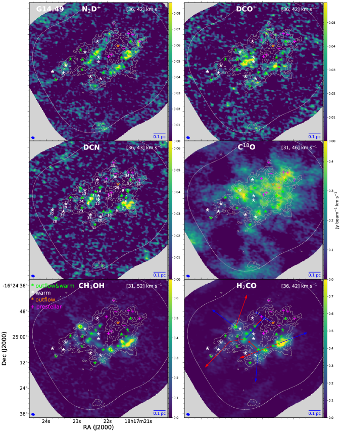
Figure 1: The velocity-integrated intensity maps of N₂D⁺, DCO⁺, DCN, C¹⁸O , CH₃OH, and H₂CO emission lines toward G14.49. The unit of the colorbar is Jy beam^-1 km s^-1. Fuchsia pluses, yellow, white, and green asterisks indicate prestellar candidates (category 1), outflow cores (category 2), warm cores (category 3), outflow+warm cores (category 4). The white dashed line shows 30% of the sensitivity level of the mosaic in the ALMA continuum image. The blue and red arrows in bottom right panel indicate directions of blue-shifted and red-shifted CO outflow lobes (see Paper II), respectively. The gray contours in each panel show the 1.3 mm continuum emission. The contour levels are (3, 6) $\times\,\sigma$, with $\sigma$ = 0.115 mJy beam^-1. The beam size of line emission and scale bar are shown in the lower left and right corner of each panel, respectively. The remaining sources are presented in the Appendix A (see Figures 10-14).

In this work, we study the chemistry of the embedded dense cores in the extremely early evolutionary stages of high-mass star-forming regions using high angular resolution and high sensitivity ALMA observations. With a statistically significant sample of dense cores, we will study the properties of deuterated molecules (N₂D⁺, DCO⁺, C₂D, and DCN) and dense gas tracers (C¹⁸O, H₂CO, CH₃OH, and ¹³CS). The paper is organized as follows: Section 2 describes the observations. The results and analysis are presented in Section 3. In Section 4 we discuss the results. A summary of the main conclusions is presented in Section 5.

2 Observations

Observations of twelve 70 $\mu$m-dark molecular clumps were performed with ALMA in Band 6 ($\sim$224 GHz; 1.34 mm) using the main 12 m array, the 7 m array, and the total power array (TP; Project ID: 2015.1.01539.S, PI: P. Sanhueza). The mosaic observations were carried out with the 12 m array and 7 m array to cover a significant portion of the clumps, as defined by single-dish continuum images. The same correlator setup was applied for all sources. More details on the observations can be found in Papers I and II.

Data calibration was performed using the CASA software package version 4.5.3, 4.6, and 4.7, while the 12 m and 7 m array datasets were concatenated and imaged together using the CASA 5.4 tclean algorithm (McMullin et al., 2007). Data cubes for lines were produced using the yclean script which automatically clean each map channel with custom made masks (Contreras et al., 2018). Two times $\sigma$ root mean square (rms) threshold is used in the imaging process. The continuum emission was obtained by averaging the line-free channels in visibility space. We used a multiscale clean for continuum and data cube, with scale values of 0, 5, 15, and 25 times the image pixel size of 0^′′.2. Since some sources were observed with different configurations, a uv-taper was used for such sources in order to obtain a similar synthesized beam of $\sim$1$\farcs$2 for all sources. We adopted a Briggs robust weighting of 0.5 and 2 for the visibilities of continuum and lines in the imaging process, respectively. This achieved an averaged 1$\sigma$ noise level of $\sim$0.1 mJy beam^-1 for the continuum images. For the detected molecular lines (N₂D⁺ $J$= 3–2, DCN $J$= 3–2, DCO⁺ $J$= 3–2, C₂D $J$= 3–2, ¹³CS $J$= 5–4, SiO $J$= 5–4, C¹⁸O $J$= 2–1, CO $J$= 2–1, CH₃OH $4_{2,2}-3_{1,2}$, and H₂CO $3_{0,3}-2_{0,2}$, $3_{2,2}-2_{2,1}$, $3_{2,1}-2_{2,0}$), the sensitivities are $\sim$9.5 mJy beam^-1 per 0.17 km s^-1 for the first six lines and $\sim$3.5 mJy beam^-1 per 1.3 km s^-1 for the last six lines (see Table 1). The 12m and 7m array line emission was combined with the TP observations through the feathering technique. All images shown in this paper are prior to the primary beam correction, while all measured fluxes are corrected for the primary beam attenuation.

3 Results and Analysis

At the moment, the ALMA TP antennas do not provide continuum emission observations. Therefore, our analysis of continuum and molecular lines is mostly focused on combined 12 m and 7 m images (hereafter 12m7m), whereas the combined 12 m, 7 m, and TP images (hereafter 12m7mTP) data are also used to assess the missing flux in images without the total power data.

The astropy astrodendro package (Rosolowsky et al., 2008; Astropy Collaboration et al., 2013) was employed to identify the embedded dense cores for each clump (Paper I). A minimum value of 2.5$\sigma$, step of 1.0$\sigma$, and a minimum number of pixels equal to those contained in half of each synthesized beam were used to extract the dense cores (i.e., the leaves in the terminology of astrodendro). To eliminate spurious detections, we only considered the cores with integrated flux densities $>$3.5$\sigma$ (see Section 4.2 in Paper I for more details on identification of dense cores).

Figure 1 shows the velocity-integrated intensity (also known as 0th-moment) maps of N₂D⁺, DCO⁺, DCN, H₂CO ($3_{0,3}-2_{0,2}$), CH₃OH, and C¹⁸O for G014.492–00.139 (hereafter G14.49), but excluding C₂D, ¹³CS, CO, and SiO. The 0th-moment images of molecular lines for the remaining clumps are presented in Appendix A. Among the three H₂CO transitions, we focus on the H₂CO ($3_{0,3}-2_{0,2}$) line, unless otherwise noted. H₂CO ($3_{0,3}-2_{0,2}$) traces cold dense gas better than the other two transitions, $3_{2,2}-2_{2,1}$ and $3_{2,1}-2_{2,0}$, which preferentially trace warm dense gas. The C₂D  and ¹³CS lines are only detected in very limited regions toward 10 dense cores. The spatial distributions of the CO and SiO lines can be found in paper II. Both the CO and C¹⁸O lines show significant emission throughout the clumps, albeit there is a significant depletion in their emission toward some dense cores. Both N₂D⁺ and DCO⁺ lines are preferentially present around or toward the dense cores. CH₃OH and H₂CO emission lines are frequently found around outflows and dense cores. The majority of DCN line emission appears toward the protostellar cores.

3.1 Detection Rates

In general, the emission from deuterated species is weak. For all the detected lines of interest, the spectra are averaged inside the dendrogram leaf (see Paper I) that defines each core in order to increase the signal-to-noise ratio (S/N). We derive the line central velocity ($v_{\rm LSR}$), observed velocity dispersion ($\sigma_{\rm obs}$ = FWHM/$2\sqrt{2\rm ln2}$), and peak intensity ($I$) from Gaussian fittings to the core-averaged spectrum for each line, except for N₂D⁺ that is fitted with hyperfine structure (hfs) model. The derived $\sigma_{\rm obs}$ is not corrected by the smearing effect due to the channel width. To increase the S/N of weak line emission, the core-averaged spectrum is spectrally smoothed over 2 native channels prior to Gaussian/hfs fittings if it shows marginal $\sim$3$\sigma$ confidence in the native spectral resolution. The best-fit parameters, that are used to compute column densities of molecules (see Appendix C) and the following analyses, are summarized in Appendix A.

The CO emission is detected in all the identified cores. C¹⁸O is detected in 267 out of the 294 cores, with a detection rate of 89%. H₂CO is the third most commonly detected line, which is detected in 156 out of the 294 cores, with a detection rate of 52%. CH₃OH is detected in 51 out of the 294 cores, leading to a detection rate of 17%. Among the detected deuterated species, DCO⁺ is the most commonly detected line with a detection rate of 39% (116/294). N₂D⁺ is detected in 54 out of the 294 cores, resulting in a detection rate of 18%. There are 7 cores associated with the DCN line emission, with a detection rate of 2%. There is weak C₂D emission in 3 dense cores, with a detection rate of 1%. ¹³CS is detected toward 4 dense cores, with a detection rate of 1%. Based on the core-averaged spectra, the SiO emission is detected in 27 cores.

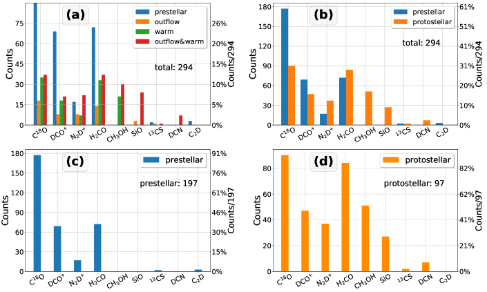
Figure 2: Histograms of number and detection rate distributions of detected lines for: each evolutionary category of cores (Panel a); prestellar vs protostellar cores (Panel b); the prestellar cores only (Panel c); the protostellar cores only (Panel d).

Figure 2 shows the histograms of the number distributions and detection rates of detected lines for the prestellar, protostellar cores, and for each core category. N₂D⁺ is detected in 17 prestellar cores and 37 protostellar cores, resulting in a detection rate in the prestellar phase lower (9% = 17/197) than that in the protostellar phase (38% = 37/97). The high N₂D⁺ detection rate for the protostellar cores indicates that N₂D⁺ does not exclusively trace prestellar cores and that it also frequently appears in the protostellar cores (Giannetti et al., 2019). Among the detected deuterated molecules, the DCO⁺ has the highest detection rate in both the prestellar and protostellar cores. The DCO⁺ detection rates are 35% (69/197) and 49% (47/97) for the prestellar and protostellar cores (Figure 2), respectively. This indicates that DCO⁺ is more frequently detected than N₂D⁺ in both the prestellar and protostellar cores.

The H₂CO detection rate in the protostellar cores (87% = 84/97) is more than twice of that in the prestellar cores (37% = 72/197). On the other hand, H₂CO has a higher detection rate than N₂D⁺ in both the prestellar and protostellar cores, indicating that H₂CO is more commonly seen than the N₂D⁺ emission in these dense cores at early evolutionary phases. There are 51 (53% = 51/97) protostellar cores showing CH₃OH line emission. DCN is detected in 7 protostellar cores. C₂D is detected in 3 prestellar cores. ¹³CS is detected in 2 prestellar and 2 protostellar cores. The detection numbers and detection rates of each line in all of the categories are summarized in Table 2.

Figure 3: Integrated intensity correlation matrix, showing cross correlations for each pair of molecules. The correlation coefficients are described in the text. The ‘+’ symbols mean that correlation coefficients can not be derived, because of either without detection or the spatially overlapped emitting area is smaller than 1 beam size. The color indicates the number of beam areas of the spatial overlapped emitting regions. A larger number of beam areas has a more robust derived correlation coefficient than a smaller one.

3.2 Spatial Distributions of Line Emission

In general, both CO and C¹⁸O show the most spatially extended emission over all clumps, followed by H₂CO and CH₃OH, and then by DCO⁺, N₂D⁺, SiO, DCN, ¹³CS, and C₂D. From Figure 1 (see also Appendix A), we note that the C¹⁸O emission is extended in the IRDC clumps. There is very weak C¹⁸O emission toward some of the dense cores likely due to depletion (e.g., cores #28/30 in G14.49; see also Sabatini et al. 2022, subm).

N₂D⁺ shows extended emission toward the dense cores. Peaks of the N₂D⁺ emission are offset from the continuum peaks in some cores, with a significant decrease in intensity toward the continuum emission peaks (e.g., cores #8/2 in G14.49; see Figure 1). Both N₂ depletion and CO evaporation toward the central of the cores can lead to decrease N₂D⁺ abundance. We are unable to distinguish between these two possibilities with the current data. DCO⁺ also shows extended emission toward the dense cores. However, the spatial distribution of DCO⁺ does not always coincide with that of N₂D⁺ (see, for example, Sakai et al., 2022). For instance, DCO⁺ shows a significantly different spatial distribution from what is observed for N₂D⁺ around cores #7/10/21 in G14.49 (see Figure 1).

The peaks of the H₂CO and CH₃OH emission appear to either coincide with the continuum peaks or locate at the direction of outflows in the majority of cases (Figures 1 and Appendix A). The CH₃OH emission shows a behavior similar to what is observed for H₂CO, but with less extended emission. This is most likely due to the fact that the excitation conditions of H₂CO ($3_{0,3}-2_{0,2}$) are different from those of CH₃OH (e.g., lower upper level energies and critical densities; see Table 1).

There are some pairs of molecules showing similar spatial distribution in some clumps, e.g., H₂CO and CH₃OH. To compare the spatial trends of different species, we performed a 1/2-beam sampling for the 0th-moment of each molecular line. Each data point (or pixel) is about 1/2 beam width, to ensure that data points are not over sampled. The similarity of the 0th-moment maps of different molecules can be evaluated quantitatively by the cross correlation between each pair of maps according to (Guzmán et al., 2018)

$$\rho_{12}=\frac{\sum\limits_{i,j}I_{1,ij}\,I_{2,ij}\,w_{ij}}{\left(\sum\limits_{i,j}I_{1,ij}^{2}\,w_{ij}\,\sum\limits_{i,j}I_{2,ij}^{2}\,w_{ij}\right)^{1/2}},$$ (1)

where the sums are taken over all positions. $I_{1,ij}$ and $I_{2,ij}$ are the integrated intensities at the position $i$, $j$ for two arbitrary species 1 and 2, respectively, and the weight $w_{ij}$ is equal to 0 or 1 depending on whether or not the line emission was detected at that position. $\rho_{12}$ is equal to 1 if the 0th-moment maps of two molecules have the same spatial distribution. Although some pairs of molecules that show weak emission do not have statistically significant number of independent data points, it is still worth an examination. To alleviate the effect of insufficient numbers of independent data points for comparison, we avoid deriving the correlation coefficient of the pair of molecules whose overlapped emitting area is smaller than 1 synthesized beam.

Figure 3 presents cross correlation coefficients for the 0th-moment map of each pair of molecules. The correlation between N₂D⁺ and DCO⁺ is better than those of the other detected deuterated molecules (i.e., DCN and C₂D) in all the clumps. This is because the emitting regions of DCN and C₂D lines are smaller than either N₂D⁺ or DCO⁺ (Figure 1). The DCO⁺ line emission coincides better with H₂CO and CH₃OH than N₂D⁺ in terms of spatial distribution. This may be because DCO⁺, H₂CO and CH₃OH have a common precursor molecule of CO that tends to destroy N₂D⁺ (see Sections 4.2 and 4.3).

In general, the CH₃OH and H₂CO emission have the most similar spatial distributions in integrated intensities with the highest correlation coefficient among the detected lines. Most of the CH₃OH and H₂CO emission appear to be around either outflows or dense cores (Figure 1). In addition, both the CH₃OH and H₂CO emission show a good spatial correlation with the SiO emission in most of the clumps (Figure 3). These results suggest that both the CH₃OH and H₂CO line emission are closely related to outflow activity toward protostellar cores in the ASHES clumps.

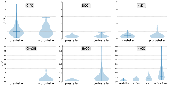
Figure 4: Violin plots of the peak intensity $I$ and observed velocity dispersion $\sigma_{\rm obs}$ distributions for each line. The shape of each distribution shows the probability density of the data smoothed by a kernel density estimator. The last panel shows the H₂CO peak intensity distributions of each category of the dense cores. The blue horizontal bars from the top to bottom in each violin plot represent the maximum, mean, and minimum values, respectively.

3.3 Molecular Line Parameters

Figure 4 shows the distribution of the derived $I$ and $\sigma_{\rm obs}$ of each line for the prestellar and protostellar cores (see also Table 3). Overall, $\sigma_{\rm obs}$ shows no significant difference between the prestellar and protostellar cores for the C¹⁸O and DCO⁺ emission. This indicates that the protostellar cores are still at a very early evolutionary phase, in which the line widths of C¹⁸O (a low density gas tracer) and DCO⁺ (a high density tracer) have not been significantly affected by protostellar activity. In general, N₂D⁺ line has comparable $I$ in both the prestellar and protostellar cores, except for 4 protostellar cores that present a relatively higher $I$ than that of prestellar cores. On the other hand, N₂D⁺ line emission shows relatively larger $\sigma_{\rm obs}$ in the protostellar cores compared with the prestellar cores. This might be because the N₂D⁺ line emission toward protostellar cores is influenced by the injection of turbulence as a result of protostellar activity.

For H₂CO emission, both $I$ and $\sigma_{\rm obs}$ in the protostellar cores are higher than in the prestellar cores. This is because H₂CO abundances can be significantly enhanced in warm and dense environments, and its line width can be broadened by protostellar activity (e.g., outflow; Tafalla et al., 2010; Sakai et al., 2012). In addition, H₂CO is the molecule in our sample that shows a clearly increasing trend in both $I$ and $\sigma_{\rm obs}$ from categories 1 to 4 (see Figure 4), indicating that its abundance and line width are sensitive to the evolution of the dense cores. This implies that H₂CO could be used as a diagnostic tool to infer star formation activities.

From Figure 4, one notes that the H₂CO ($\langle\sigma_{\rm obs}\rangle$ = 1.68 km s^-1) and CH₃OH ($\langle\sigma_{\rm obs}\rangle$ = 1.82 km s^-1) lines show relatively larger $\sigma_{\rm obs}$ than C¹⁸O ($\langle\sigma_{\rm obs}\rangle$ = 0.99 km s^-1), DCO⁺ ($\langle\sigma_{\rm obs}\rangle$ = 0.35 km s^-1), and N₂D⁺ ($\langle\sigma_{\rm obs}\rangle$ = 0.25 km s^-1) toward the protostellar cores (see also Table 3). This could be because H₂CO and CH₃OH are associated with more turbulent gas components affected by protostellar activity (e.g., outflow; Tychoniec et al., 2021). We refrain from investigating $I$ and $\sigma_{\rm obs}$ for the ¹³CS, DCN, and C₂D emission due to a lack of a sufficient number of detections for a meaningful analysis, as well as the SiO emission that is mainly associated with outflows.

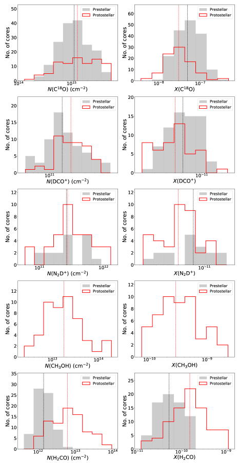
Figure 5: Left column: histograms of the molecular column densities for the prestellar and protostellar cores. Right column: histograms of the molecular abundances for the prestellar and protostellar cores. The black dashed vertical lines indicate the median values of the parameters.

3.4 Derivation of Physical Parameters

The rotational excitation temperature ($T_{\rm NH_{3}}$) is derived from NH₃ (1, 1) and (2, 2) transition lines obtained from the CACHMC survey (Complete ATCA Census of High-Mass Clumps; Allingham et al., 2022 in prep) at $\sim$5^′′ angular resolution (see Appendix B for detailed procedure on excitation temperature determination). More details procedure on temperature determination and survey results will be presented in a forthcoming paper (Allingham et al., in prep). The derived $T_{\rm NH_{3}}$ is used as excitation temperature in the calculation of all molecular parameters, except for G332.96 that has no available NH₃ data. We used the dust temperature at the clump scale of 12.6 K for G332.96 (Paper I). The averaged temperature of dense cores in the same category for a given clump is used for those dense cores that have no available $T_{\rm NH_{3}}$. The approximation of using $T_{\rm NH_{3}}$ as the excitation temperature is based on the LTE conditions in calculation of molecular density. The results could be highly sensitivity to the choice of the excitation temperature.

Using these new temperatures, we have recalculated the ASHES cores properties. The analysis on how these new core properties affect the analysis presented in Sanhueza et al. (2019) will be presented in a forthcoming paper (Li et al. 2022, in prep). For the chemical analysis of the current work, we have used the updated core-average H₂ column densities and core volume densities (see Appendix C). The updated parameters are 4.9 $\times$ 10²¹–2.0 $\times$ 10²³ cm^-2 for the core-averaged column density and 1.4 $\times$ 10⁵–1.7 $\times$ 10⁷ cm^-3 for the core-averaged volume density. The protostellar cores have higher column densities and volume densities than the prestellar cores (Table 4).

Assuming local thermodynamic equilibrium (LTE) and optically thin molecular emission, the molecular column density ($N_{\rm mol}$) can be estimated from the velocity integrated intensity (see Appendix C, for a detailed derivation of the column density). To study the properties of the molecules, we also calculated the molecular abundances, $X_{\rm mol}=N_{\rm mol}/N_{\rm H_{2}}$, using the updated H₂ column density and derived molecular column densities.

The derived N₂D⁺ column densities range from 5.9 $\times$ 10¹⁰ to 1.3 $\times$ 10¹² cm^-2, resulting in N₂D⁺ abundances of 2.2 $\times$ 10^-12–1.7 $\times$ 10^-11. The N₂D⁺ column densities are similar to the value of 6.2 $\times$ 10¹¹ cm^-2 obtained for other IRDCs (e.g., Gerner et al., 2015; Barnes et al., 2016; Chen et al., 2010), and the N₂D⁺ abundances are comparable to the values of $\sim$10^-12 in other massive clumps (Giannetti et al., 2019). The estimated DCO⁺ column densities are between 4.7 $\times$ 10¹⁰ and 6.5 $\times$ 10¹¹ cm^-2, leading to DCO⁺ abundances of 1.3 $\times$ 10^-12–2.4 $\times$ 10^-11. $N_{\rm DCO^{+}}$ is similar to the values reported in other IRDCs ($\leqslant$3 $\times$ 10¹¹ cm^-2 Gerner et al., 2015). The derived DCN column densities and abundances are 2.7 $\times$ 10¹¹–2.0 $\times$ 10¹² cm^-2 and 5.6 $\times$ 10^-12–1.2 $\times$ 10^-11, respectively. The DCN abundances are significantly lower than those in more evolved dense cores in W3 ($>$10^-10; Mottram et al., 2020). C₂D has column densities of 4.8 $\times$ 10¹²–1.1 $\times$ 10¹³ cm^-2 and abundances of 1.5 $\times$ 10^-10–4.2 $\times$ 10^-10.

Given that these dense cores are still in very early evolutionary phases and are characterized by a cold environment, H₂CO is expected to form in ice on the grain surface and subsequently to be released to the gas phase (Jørgensen et al., 2005). We assumed an ortho-to-para ratio of 1.6 which is consistent with thermalization at a low temperature of T $\sim$ 15 K (Jørgensen et al., 2005). The derived H₂CO column densities and abundances are 4.1 $\times$ 10¹¹–9.3 $\times$ 10¹³ cm^-2 and 1.2 $\times$ 10^-11–1.1 $\times$ 10^-9, respectively. CH₃OH has column densities of 2.4 $\times$ 10¹²–1.9 $\times$ 10¹⁴ cm^-2 and abundances of 7.3 $\times$ 10^-11–2.3 $\times$ 10^-9 for the detected dense cores. The abundances of H₂CO and CH₃OH are similar to those in dense cores prior to the hot core phase in other IRDCs (a few 10^-10 for H₂CO and CH₃OH; Gerner et al., 2014; Mottram et al., 2020), but lower than those in hot core and UCHII regions ($\geqslant$10^-9; e.g., Gerner et al., 2014; Mottram et al., 2020).

C¹⁸O optical correction factor, $C_{\tau}=\tau_{\rm C^{18}O}/[1-\rm{exp}(-\tau_{\rm C^{18}O})]$, is applied in the calculation of C¹⁸O column density. $C_{\tau}$ is derived following the approach described in Sabatini et al. (2019). The detailed estimation of C¹⁸O correction factor is presented in Sabatini et al. (2022). The calculated C¹⁸O column densities vary from 1.3 $\times$ 10¹⁴ to 5.6 $\times$ 10¹⁵ cm^-2, resulting in C¹⁸O abundances of 3.7 $\times$ 10^-9–4.8 $\times$ 10^-7. The estimated SiO column densities vary from 2.3 $\times$ 10¹¹–3.2 $\times$ 10¹³ cm^-2 that are comparable to the values in outflows, whereas the derived abundances of 3.0 $\times$ 10^-12–3.4 $\times$ 10^-10 are lower than those found in outflows ($\geqslant$1.1 $\times$ 10^-9; see Paper II).

Figure 5 shows histograms of molecular column densities and abundance ratio distributions for the prestellar and protostellar cores (see also Table 4). Except for C¹⁸O and N₂D⁺ that have a similar column density in the prestellar and protostellar cores, all other molecules have column densities in the prestellar cores relatively lower than those from protostellar cores. On the other hand, N₂D⁺, DCO⁺, and C¹⁸O abundances are higher in the prestellar cores than in the protostellar cores, indicating that the abundances of these molecules tend to decrease with the evolution of the dense cores. These abundance variations are dominated by the effect of the H₂ density increase rapidly from prestellar to protostellar phases (see Section 4.2). In contrast, the abundance of H₂CO in the protostellar cores is higher than in the prestellar ones, suggesting that its abundance can be enhanced with core evolution.

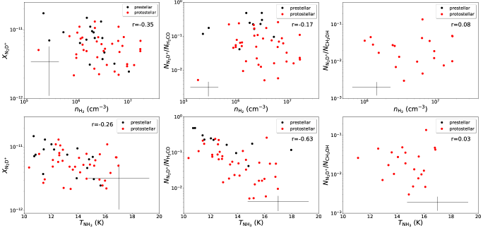
Figure 6: Top row: plots of $N_{\rm H_{2}}$ versus $N_{\rm N_{2}D^{+}}$, $N_{\rm N_{2}D^{+}}/N_{\rm H_{2}CO}$, and $N_{\rm N_{2}D^{+}}/N_{\rm CH_{3}OH}$. Bottom row: plots of $T_{\rm NH_{3}}$ versus $X_{\rm N_{2}D^{+}}$, $N_{\rm N_{2}D^{+}}/N_{\rm H_{2}CO}$, and $N_{\rm N_{2}D^{+}}/N_{\rm CH_{3}OH}$. The correlation coefficients derived from the Spearman rank correlation test are texted in each panel. The black cross shows the typical uncertainty in each panel.

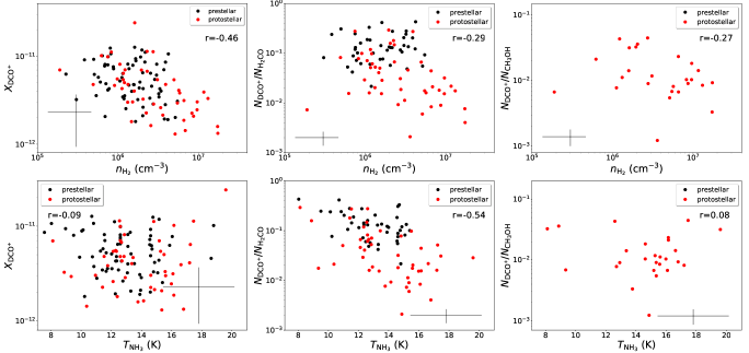
Figure 7: Same as Figure 6, but for the DCO⁺.

4 Discussion

4.1 Missing flux

To understand the impact of the missing flux on the line emission, we compared the 12m7m and 12m7mTP datasets. We investigated the integrated intensities, peak intensities, line widths, and central velocities of line emission between the two datasets.

For the N₂D⁺ line emission, we find that the 12m7m data have recovered about 92% of the 12m7mTP flux. The differences of the measured $I$ and $\sigma_{\rm obs}$ are a factor of 0.94 and 0.99, respectively. For the DCO⁺ line emission, the mean ratios of 12m7m to 12m7mTP are 0.89 for $I$ and 0.9 for $\sigma_{\rm obs}$, resulting a mean flux ratio (velocity integrated intensity) of 0.79. The DCO⁺ emission behaviour is very similar to that of N₂D⁺. These results indicate that most of the N₂D⁺ and DCO⁺ emission is compact and recovered without the addition of total power data from single-dish telescopes.

For the H₂CO ($3_{0,3}-2_{0,2}$) line emission, the 12m7m data recover about 71% of the 12m7mTP flux, and the mean ratios of 12m7m to 12m7mTP for $I$ and $\sigma_{\rm obs}$ are 0.82 and 0.87, respectively. On other hand, CH₃OH has similar flux, $I$, and $\sigma_{\rm obs}$ between the 12m7m and 12m7mTP datasets; the mean ratio (12m7m/12m7mTP) is 0.94 for flux, 0.94 for $I$, and 1.0 for $\sigma_{\rm obs}$. This indicates that CH₃OH traces more spatially compact emission compared with H₂CO. This suggests that the observed CH₃OH transition may preferentially be concentrated near the protostars or in knots in outflows.

For C¹⁸O, the mean ratios of 12m7m to 12m7mTP data are 0.54 for the intensity peak and 0.7 for the velocity dispersion, resulting a mean flux ratio of 0.36. Among the detected lines (except for CO), C¹⁸O suffers most severely from missing flux. This indicates that C¹⁸O probes a significant amount of diffuse molecular gas. For the remaining lines with relatively low detection rates, their 12m7m images are weakly affected by missing flux. The mean flux ratios of 12m7m to 12m7mTP are 1.0 for SiO, 0.96 for ¹³CS, 0.9 for DCN, and 0.98 for C₂D.

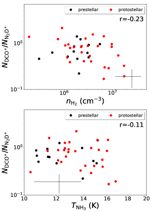
Figure 8: The column density ratio of DCO⁺ to N₂D⁺ versus the core-averaged volume density $n_{\rm H_{2}}$ and the temperature $T_{\rm NH_{3}}$.

4.2 Deuterated Molecules

N₂D⁺ is expected to be abundant in cold ($<$20 K) and dense ($\sim$10${}^{5}\rm\,cm^{-3}$) regions, in which its major destroyer, CO, is significantly depleted onto grain surfaces. N₂D⁺ can be formed via N₂ reacting with H₂D⁺ (dominant reaction: N₂ + H₂D⁺ $\rightarrow$ N₂D⁺ + H₂), D₂H⁺, or D₃⁺ (Pagani et al., 2009), and destroyed by CO (N₂D⁺ + CO $\rightarrow$ DCO⁺ + N₂) or electrons (N₂D⁺ + e^- $\rightarrow$ ND +N or D + N₂; Sakai et al., 2022). DCO⁺ is also considered as a cold and dense gas tracer. However, DCO⁺ requires gas-phase CO for its formation at cold temperatures (T $<$ 20–50 K), i.e., H₂D⁺ + CO $\rightarrow$ DCO⁺ + H₂ (Wootten & Loren, 1987). Therefore, the DCO⁺ abundance does not decrease rapidly when CO is released to the gas phase from the grain mantles (Dalgarno & Lepp, 1984). The different chemistry between N₂D⁺ and DCO⁺ may explain their different spatial distributions seen in Figure 1 (e.g., Sakai et al., 2022). DCN and C₂D tend to form in warm environments (Turner, 2001; Albertsson et al., 2013).

N₂D⁺ and DCO⁺ column densities exhibit a strong correlation (see Figure 15 in Appendix A), with a Spearman’s rank correlation coefficient of $r$ = 0.58. This is mostly because both lines trace cold and dense gas in the dense cores. The N₂D⁺ abundance appears to decrease with increasing volume densities $n_{\rm H_{2}}$, with a moderate correlation coefficient of -0.35 (see Figures 6). As mentioned in Section 3.4, the volume density increases with the evolution of the dense cores that continue to accumulate mass via accretion of material from the natal clumps. The $n_{\rm H_{2}}$–$X_{\rm N_{2}D^{+}}$ anticorrelation suggests that the N₂D⁺ abundance decreases with the core evolution. As the cores evolve, the gas temperature increases, thereby lowering the deuterium enhancement. In this case, one naively expects an anticorrelation between N₂D⁺ abundance and $T_{\rm NH_{3}}$. As seen in Figures 6, there is no obvious trend between the N₂D⁺ abundance and $T_{\rm NH_{3}}$. These cores are still very cold with temperatures between 10 and 20 K, which are lower than the sublimation temperature of CO ($\sim$25 K). This may explain why the N₂D⁺ abundance does not vary significantly with $T_{\rm NH_{3}}$. In addition, this suggests that these cores are still at a very early evolutionary phase, in which the surrounding environment has not been significantly warmed up by the young stellar objects (YSOs). On the other hand, we cannot completely rule out the possibility that $T_{\rm NH_{3}}$ does not accurately reflect the true temperature of the dense molecular gas traced by N₂D⁺, because the spatial resolution of $T_{\rm NH_{3}}$ ($\sim$5^′′) is coarser than the ALMA observations ($\sim$1.2^′′) and the critical density of NH₃ (1,1) is only of a few 10⁴ cm^-3. Determination of temperatures at $\sim$1^′′ scales would be necessary to verify whether the $T_{\rm NH_{3}}$ varies significantly down to the small scale. The $n_{\rm H_{2}}$–$X_{\rm N_{2}D^{+}}$ and $X_{\rm N_{2}D^{+}}$– $T_{\rm NH_{3}}$ results suggest that the N₂D⁺ abundance variation is dominated by the H₂ core density in the ASHES sample.

The column density ratio of $N_{\rm N_{2}D^{+}}$/$N_{\rm H_{2}CO}$ appears to decrease as a function of increasing $n_{\rm H_{2}}$. However, a closer look reveals that this weak anticorrelation is mostly dominated by the protostellar cores. Both $N_{\rm N_{2}D^{+}}$ and $N_{\rm H_{2}CO}$ tend to increase with $n_{\rm H_{2}}$, and therefore, the $N_{\rm N_{2}D^{+}}$/$N_{\rm H_{2}CO}$-$n_{\rm H_{2}}$ anticorrelation implies that $N_{\rm H_{2}CO}$ is more sensitive to $n_{\rm H_{2}}$ than $N_{\rm N_{2}D^{+}}$ toward the protostellar cores (see also Section 3.3). In addition, the ratio $N_{\rm N_{2}D^{+}}$/$N_{\rm H_{2}CO}$ also appears to decrease with increasing $T_{\rm NH_{3}}$, with a correlation coefficient of -0.63. This is because the H₂CO abundance is enhanced by elevated temperatures. The $N_{\rm N_{2}D^{+}}$/$N_{\rm CH_{3}OH}$ ratio shows no clear trend with $n_{\rm H_{2}}$ or $T_{\rm NH_{3}}$. In general, DCO⁺ shows a similar trend to those seen in N₂D⁺, except for $n_{\rm H_{2}}$–$N_{\rm DCO^{+}}$/$N_{\rm CH_{3}OH}$ ($r$ = -0.27) that presents a weak anticorrelation. The difference in N₂D⁺ and DCO⁺ may be a result of different chemistry.

There is a weak anticorrelation between $n_{\rm H_{2}}$ and the $N_{\rm DCO^{+}}$/$N_{\rm N_{2}D^{+}}$ ratio (see Figure 8), with a correlation coefficient of $r$ = -0.23. From Figures 6 and 7, one notes that both N₂D⁺ and DCO⁺ abundances decrease with increasing $n_{\rm H_{2}}$, thereby causing the ratio of DCO⁺ to N₂D⁺ to slightly change with $n_{\rm H_{2}}$. In addition, the $N_{\rm DCO^{+}}$/$N_{\rm N_{2}D^{+}}$ ratio shows only minor changes with $T_{\rm NH_{3}}$, which gives a correlation coefficient of $r$ = -0.11. This can be ascribed to the fact that the both DCO⁺ and N₂D⁺ abundances do not vary significantly with $T_{\rm NH_{3}}$ (see Figures 6 and 7).

4.3 H₂CO and CH₃OH

CH₃OH is considered to be mostly formed on the surface of dust grains via the hydrogenation of CO with some intermediate products (e.g., H₂CO; Charnley et al., 1997; Watanabe et al., 2004; Fuchs et al., 2009),

$$\rm CO\;\xrightarrow[\text{H}]{\;}HCO\xrightarrow[\text{H}]{\;}H_{2}CO\xrightarrow[\text{H}]{\;}CH_{2}OH,CH_{3}O\xrightarrow[\text{H}]{\;}CH_{3}OH.$$ (2)

Unlike CH₃OH, which formed entirely on the surfaces of dust grains, H₂CO can be formed efficiently through both grain-surface reaction in cold environments and gas-phase reactions in warm/hot environments (Le Teuff et al., 2000; Garrod et al., 2006; Fuchs et al., 2009).

CH₃OH shows a dip in its emission distribution at the center of some dense cores, such as the protostellar core #15 in G337.54 (Appendix A). A similar feature has been observed in low-mass prestellar cores, e.g., L1498 and L1517B (Tafalla et al., 2006). These authors suggest that the weaker CH₃OH emission toward the center of the dense cores is due to the significant CH₃OH depletion in the cold and dense environments. Therefore, the low detection rate of CH₃OH in the dense cores may be partly ascribed to CH₃OH depletion.

Among the detected molecules, H₂CO and CH₃OH column densities show the strongest correlation, with a correlation coefficient of 0.83 (see Figure 15 in Appendix A). As mentioned in Section 3.3, both H₂CO and CH₃OH tend to probe the dense and high velocity molecular gas, and hence, the protostellar activity may be partly responsible for the strong correlation of the two species. For example, outflow/shocks can release both H₂CO and CH₃OH from grain mantles to the gas phase. In addition, both H₂CO and CH₃OH column densities show strong correlation with the SiO column density (see Figure 15 in Appendix A); the correlation coefficient is 0.73 for $N_{\rm H_{2}CO}$–$N_{\rm SiO}$ and 0.84 for $N_{\rm CH_{3}OH}$–$N_{\rm SiO}$.

The derived abundance ratios of H₂CO/CH₃OH = 0.1–2.3 are comparable to the values of 0.9–2.5 reported in dense clumps ($n_{\rm H_{2}}\sim$ 10⁶ cm^-3; Leurini et al., 2010), hot-corinos (0.7–4.3; Maret et al., 2004, 2005), and low-mass starless cores (1.1–2.2; e.g., L1498 and L1517B; Tafalla et al., 2006). These values are higher than the abundance ratios derived in hot cores (0.13–0.28; Bisschop et al., 2007) and shocked gas in the Galactic Center clouds (0.01-0.1; Requena-Torres et al., 2006; Lu et al., 2021), whereas they are significantly lower than those in the inter-clump medium (H₂CO/CH₃OH = 14–1400; $n_{\rm H_{2}}\sim$ 10⁴ cm^-3; Leurini et al., 2010). The discrepancies could be attributed to either different dominant formation mechanisms or different chemical conditions. A detailed chemical modeling and observational comparison is needed to distinguish between these possibilities, which is beyond the scope of this paper.

5 Conclusion

In this paper, we analyze ALMA data from the ASHES project to investigate the chemistry of 294 dense cores in 12 massive 70 $\mu$m dark clumps. We have studied the spatial distributions and chemical variations of C¹⁸O, DCO⁺, N₂D⁺, DCN, C₂D   H₂CO, CH₃OH, ¹³CS, and SiO in different evolutionary phases of dense cores. The main results are summarized below.

• The detection rates of the DCO⁺ emission in the prestellar and protostellar cores are higher than those of N₂D⁺, whereas N₂D⁺ is more sensitive to the core evolution than DCO⁺ in terms of the clear variations of $\sigma_{\rm obs}$. The commonly detected DCO⁺ emission toward deeply embedded dense cores suggests that it is a good tracer of prestellar (detection rate 35%) and early phase protostellar cores (detection rate 49%). On the other hand, we find that N₂D⁺ does not exclusively trace the prestellar cores and it is more frequently detected in the relatively earlier phase of the protostellar cores; the detection rate is 9% for the prestellar cores and 38% for the protostellar cores. This suggests that N₂D⁺ is not the best tracer of prestellar cores at the sensitivity obtained in ASHES.

• Both N₂D⁺ and DCO⁺ abundances decrease with the core evolution. This is mainly caused by the effects of the H₂ density increasing rapidly and the temperature increasing slowly from the prestellar to protostellar phases in the identified cores. This can also explain that the C¹⁸O abundance is higher in the prestellar cores than in the protostellar cores.

• The detection rate of the H₂CO emission toward dense cores is 52%, three times higher than that of CH₃OH (17%). The high detection rates of H₂CO in both the prestellar (37%) and protostellar cores (87%) suggest that H₂CO is commonly seen in the very early evolutionary phase. The line widths of H₂CO are higher than those of C¹⁸O, N₂D⁺, and DCO⁺ toward the protostellar cores, which is likely due to the fact that the H₂CO line is associated with more turbulent gas components related to protostellar activities (e.g., outflows). The H₂CO abundances are found to increase with the evolution of the dense cores, as well as the line intensity and line width of H₂CO ($3_{0,3}-2_{0,2}$) transition. These results indicate that H₂CO could be used as a diagnostic tool to inferring star formation activities.

Table 1: Summary of detected lines and their parameters.

Molecule	Transition	Frequency	E${}_{u}/k$	$S_{ij}\mu^{2}$	$n_{\rm crit}$	$Q_{\rm rot}$	Rotational Constants	Beam Size	rms
		(GHz)	(K)	D2	(cm-3)		(MHz)	(′′)
DCO+	$3-2$	216.112	20.74	45.624	1.84E+06	0.58$T_{\rm ex}$ + 0.34		1.5 $\times$ 1.0	9.5a
C2D	$3-2$	216.373	20.77	2.541	8.18E+05	3.47$T_{\rm ex}$ + 2.06		1.6 $\times$ 1.0	9.5a
SiO	$5-4$	217.105	14.48	48.146	1.22E+06	$\frac{k_{\rm B}T_{\rm ex}}{hB_{0}}+\frac{1}{3}$	$B_{0}$=21711.97	1.6 $\times$ 1.0	9.5a
DCN	$3-2$	217.238	20.85	80.501	2.16E+07	0.1$T_{\rm ex}^{3/2}$ + 50.51		1.7 $\times$ 1.0	9.5a
p-H2CO	3${}_{0,3}-2_{0,2}$	218.222	20.95	16.308	2.56E+06	$\frac{1}{3}\left(\frac{\pi k_{\rm B}^{3}T_{\rm ex}^{3}}{h^{3}A_{0}B_{0}C_{0}}\right)^{0.5}$	$A_{0}$ = 281970.56	1.5 $\times$ 1.0	3.5b
p-H2CO	3${}_{2,2}-2_{2,1}$	218.475	68.09	9.062	2.96E+06		$B_{0}$ = 38833.987	1.5 $\times$ 1.0	3.5b
p-H2CO	3${}_{2,1}-2_{2,0}$	218.76	68.11	9.062	3.36E+06		$C_{0}$ = 34004.244	1.5 $\times$ 1.0	3.5b
CH3OH	4${}_{2,2}-3_{1,2}$	218.44	45.46	13.906	2.04E+07	$\frac{1}{2}\left(\frac{\pi k_{\rm B}^{3}T_{\rm ex}^{3}}{h^{3}A_{0}B_{0}C_{0}}\right)^{0.5}$	$A_{0}$ = 127523.4	1.5 $\times$ 1.0	3.5b
							$B_{0}$ = 24690.2
							$C_{0}$ = 23759.7
C18O	$2-1$	219.56	15.81	0.024	9.33E+03	$\frac{k_{\rm B}T_{\rm ex}}{hB_{0}}+\frac{1}{3}$	$B_{0}$=54891.42	1.5 $\times$ 1.0	3.5b
13CS	$5-4$	231.22	32.73	38.335	4.46E+06	1.85$T_{\rm ex}$ - 3.32		1.4 $\times$ 1.0	9.5a
N2D+	$3-2$	231.321	22.2	312.104	1.70E+06	4.87$T_{\rm ex}$ + 2.81		1.5 $\times$ 1.0	9.5a

Table 2: Detection rate

Molecules	Prestellar		Protostellar			All
		Outflow Core	Warm Core	Outflow&Warm Core	Sum
Total Number	197	21	37	37	97	294
C18O	177 (89.8%)	18 (85.7%)	35 (94.6%)	37 (94.9%)	90 (92.8%)	267 (90.8%)
DCO+	69 (35.0%)	8 (38.1%)	18 (48.6%)	21 (53.8%)	47 (48.5%)	116 (39.5%)
N2D+	17 (8.6%)	8 (38.1%)	7 (18.9%)	22 (56.4%)	37 (38.1%)	54 (18.4%)
H2CO	72 (36.5%)	14 (66.7%)	33 (89.2%)	37 (94.9%)	84 (86.6%)	156 (53.1%)
CH3OH	-	-	21 (56.8%)	30 (76.9%)	51 (52.6%)	51 (17.3%)
SiO	-	3 (14.3%)	-	24 (61.5%)	27 (27.8%)	27 (9.2%)
13CS	2 (1.0%)	1 (4.8%)	-	1 (2.6%)	2 (2.1%)	4 (1.4%)
DCN	-	-	-	7 (17.9%)	7 (7.2%)	7 (2.4%)
C2D	3 (1.5%)	-	-	-	-	3 (1.0%)

Table 3: Median and mean values of derived line parameters for each category

Name	Prestellar		Protostellar								All
			Outflow Core		Warm Core		Outflow&Warm Core		Sum
	median	mean	median	mean	median	mean	median	mean	median	mean	median	mean
$I_{\rm C^{18}O}$	0.98	1.12	0.81	0.88	0.86	0.96	1.22	1.30	0.90	1.09	0.93	1.11
$\sigma_{\rm C^{18}O}$	0.75	0.89	0.88	0.95	0.92	1.02	0.85	0.97	0.88	0.99	0.79	0.92
$I_{\rm N_{2}D^{+}}$	0.41	0.42	0.29	0.31	0.52	0.47	0.44	0.53	0.40	0.47	0.41	0.45
$\sigma_{\rm N_{2}D^{+}}$	0.22	0.21	0.21	0.25	0.19	0.21	0.24	0.26	0.23	0.25	0.22	0.23
$I_{\rm DCO^{+}}$	0.32	0.37	0.37	0.46	0.33	0.37	0.36	0.37	0.35	0.39	0.33	0.38
$\sigma_{\rm DCO^{+}}$	0.29	0.30	0.29	0.29	0.38	0.39	0.32	0.35	0.32	0.35	0.30	0.32
$\sigma_{\rm CH_{3}OH}$	-	-	-	-	1.23	1.59	1.46	1.98	1.35	1.82	1.35	1.82
$I_{\rm H_{2}CO}$	0.18	0.19	0.28	0.28	0.33	0.42	0.61	0.88	0.38	0.60	0.26	0.41
$\sigma_{\rm H_{2}CO}$	0.72	0.84	0.96	1.06	1.19	1.36	1.85	2.21	1.33	1.68	1.00	1.29
$I_{\rm{}^{13}CS}$	0.38	0.38	0.27	0.27	-	-	0.18	0.18	0.22	0.22	0.28	0.30
$\sigma_{\rm{}^{13}CS}$	0.34	0.34	0.46	0.46	-	-	1.30	1.30	0.88	0.88	0.42	0.61
$I_{\rm DCN}$	-	-	-	-	-	-	0.26	0.22	0.26	0.22	0.26	0.22
$\sigma_{\rm DCN}$	-	-	-	-	-	-	1.21	1.04	1.21	1.04	1.21	1.04
$I_{\rm C_{2}D}$	0.22	0.24	-	-	-	-	-	-	-	-	0.22	0.24
$\sigma_{\rm C_{2}D}$	0.13	0.17	-	-	-	-	-	-	-	-	0.13	0.17

Table 4: Median and mean values of derived core properties for each category

Name	Prestellar		Protostellar								All
			Outflow Core		Warm Core		Outflow&Warm Core		Sum
	median	mean	median	mean	median	mean	median	mean	median	mean	median	mean
$T_{\rm NH_{3}}$(K)	14.1	14.2	12.8	13.8	14.8	14.3	15.3	14.9	14.8	14.4	14.4	14.3
		Core averaged volume densities (cm-3) and averaged column densities (cm-2)
$n_{\rm H_{2}}$	1.06E+06	1.51E+06	1.52E+06	2.50E+06	1.20E+06	2.69E+06	3.42E+06	5.28E+06	2.30E+06	3.69E+06	1.25E+06	2.23E+06
$N_{\rm H_{2}}$	2.10E+22	2.56E+22	3.25E+22	3.83E+22	2.57E+22	4.15E+22	5.64E+22	7.91E+22	4.36E+22	5.59E+22	2.56E+22	3.56E+22
				Column densities (cm-2)
$N_{\rm C^{18}O}$	1.10E+15	1.42E+15	8.35E+14	1.30E+15	1.18E+15	1.54E+15	1.79E+15	2.20E+15	1.29E+15	1.77E+15	1.16E+15	1.54E+15
$N_{\rm N_{2}D^{+}}$	2.63E+11	3.30E+11	2.28E+11	2.61E+11	3.55E+11	4.06E+11	2.96E+11	4.39E+11	2.74E+11	3.94E+11	2.72E+11	3.74E+11
$N_{\rm DCO^{+}}$	1.47E+11	1.89E+11	1.71E+11	2.12E+11	2.22E+11	2.37E+11	1.92E+11	2.05E+11	1.92E+11	2.18E+11	1.67E+11	2.01E+11
$N_{\rm CH_{3}OH}$	-	-	-	-	8.36E+12	2.09E+13	1.86E+13	3.61E+13	1.74E+13	2.98E+13	1.74E+13	2.98E+13
$N_{\rm H_{2}CO}$	1.39E+12	1.61E+12	2.84E+12	3.00E+12	4.29E+12	5.83E+12	1.20E+13	2.04E+13	6.11E+12	1.18E+13	2.43E+12	7.09E+12
$N_{\rm{}^{13}CS}$	1.14E+12	1.14E+12	1.06E+12	1.06E+12	-	-	1.89E+12	1.89E+12	1.47E+12	1.47E+12	1.29E+12	1.31E+12
$N_{\rm DCN}$	-	-	-	-	-	-	7.73E+11	1.05E+12	7.73E+11	1.05E+12	7.73E+11	1.05E+12
$N_{\rm C_{2}D}$	8.91E+12	8.33E+12	-	-	-	-	-	-	-	-	8.91E+12	8.33E+12
$N_{\rm SiO}$	-	-	1.74E+12	1.46E+12	-	-	1.70E+12	5.59E+12	1.74E+12	5.13E+12	1.74E+12	5.13E+12
					Molecular abundances
$X_{\rm C^{18}O}$	4.95E-08	6.74E-08	3.53E-08	3.68E-08	3.85E-08	6.37E-08	2.33E-08	2.95E-08	2.99E-08	4.43E-08	4.23E-08	5.96E-08
$X_{\rm N_{2}D^{+}}$	7.57E-12	8.07E-12	5.94E-12	5.99E-12	7.78E-12	7.91E-12	4.90E-12	5.07E-12	5.23E-12	5.81E-12	6.12E-12	6.52E-12
$X_{\rm DCO^{+}}$	5.23E-12	5.95E-12	4.79E-12	4.71E-12	6.58E-12	7.60E-12	2.46E-12	2.84E-12	4.02E-12	4.98E-12	4.78E-12	5.56E-12
$X_{\rm CH_{3}OH}$	-	-	-	-	2.75E-10	4.44E-10	3.00E-10	4.72E-10	2.83E-10	4.60E-10	2.83E-10	4.60E-10
$X_{\rm H_{2}CO}$	5.20E-11	6.88E-11	8.09E-11	8.74E-11	1.59E-10	2.40E-10	1.76E-10	2.80E-10	1.53E-10	2.32E-10	8.87E-11	1.57E-10
$X_{\rm{}^{13}CS}$	6.03E-11	6.03E-11	7.94E-11	7.94E-11	-	-	1.52E-11	1.52E-11	4.73E-11	4.73E-11	5.41E-11	5.38E-11
$X_{\rm DCN}$	-	-	-	-	-	-	8.30E-12	8.55E-12	8.30E-12	8.55E-12	8.30E-12	8.55E-12
$X_{\rm C_{2}D}$	1.79E-10	2.50E-10	-	-	-	-	-	-	-	-	1.79E-10	2.50E-10
$X_{\rm SiO}$	-	-	4.05E-11	4.38E-11	-	-	3.26E-11	5.69E-11	3.35E-11	5.54E-11	3.35E-11	5.54E-11

Appendix A Additional Figures and Table

Figure 9 shows the core-averaged spectra of the detected molecular lines in G14.49 as examples. Figures 10-14 shows velocity-integrated intensity maps of N₂D⁺, DCO⁺, DCN, H₂CO, CH₃OH, and C¹⁸O lines emission for each clump. Figure 15 shows the correlation of each pair of molecular column densities. Table 5 summaries the derived parameters of detected lines.

Figure 9: Examples of core-averaged spectra of C¹⁸O, DCO⁺, N₂D⁺, H₂CO, CH₃OH, and SiO for core #7 in G14.49.

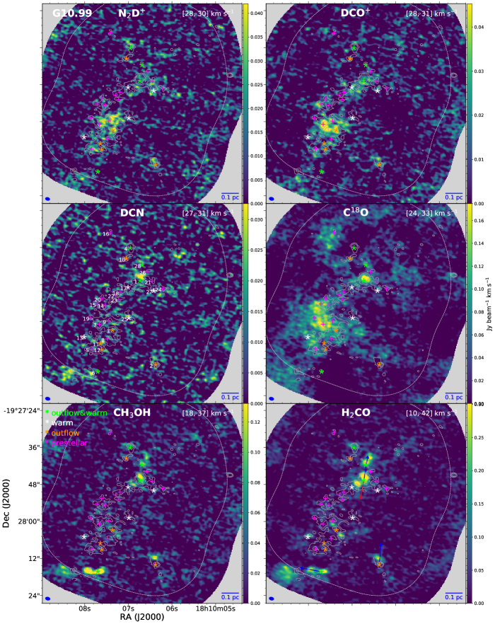
Figure 10: The velocity-integrated intensity maps of N₂D⁺, DCO⁺, DCN, C¹⁸O , CH₃OH, and H₂CO emission lines toward G10.99. Fuchsia plusses, yellow, white, and Green asterisks symbols indicate prestellar candidates (category 1), outflow cores (category 2), warm cores (category 3), and outflow+warm cores (category 4). The white dashed line shows 30% of the sensitivity level of the mosaic in the ALMA continuum image. The blue and red arrows in middle right panel indicate directions of the blueshifted and redshifted CO outflow lobes (see Paper II), respectively. The gray contours in each panel shows the 1.3 mm continuum emission. The contour levels are (3, 6) $\times\,\sigma$ , with $\sigma$ = 0.115 mJy beam^-1. The beam size is shown in the lower left corner of each panel.

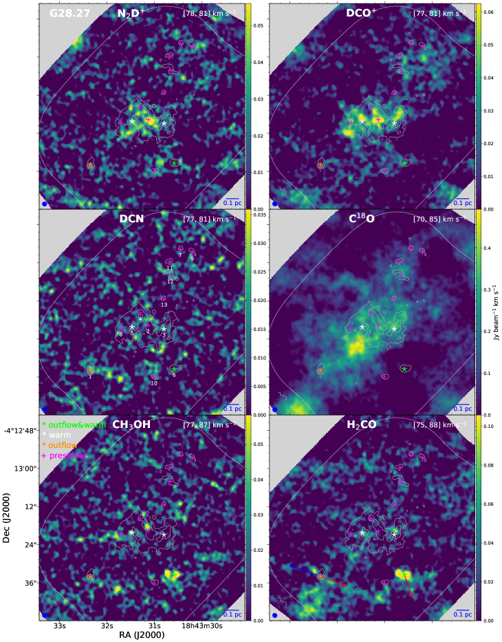
Figure 10:

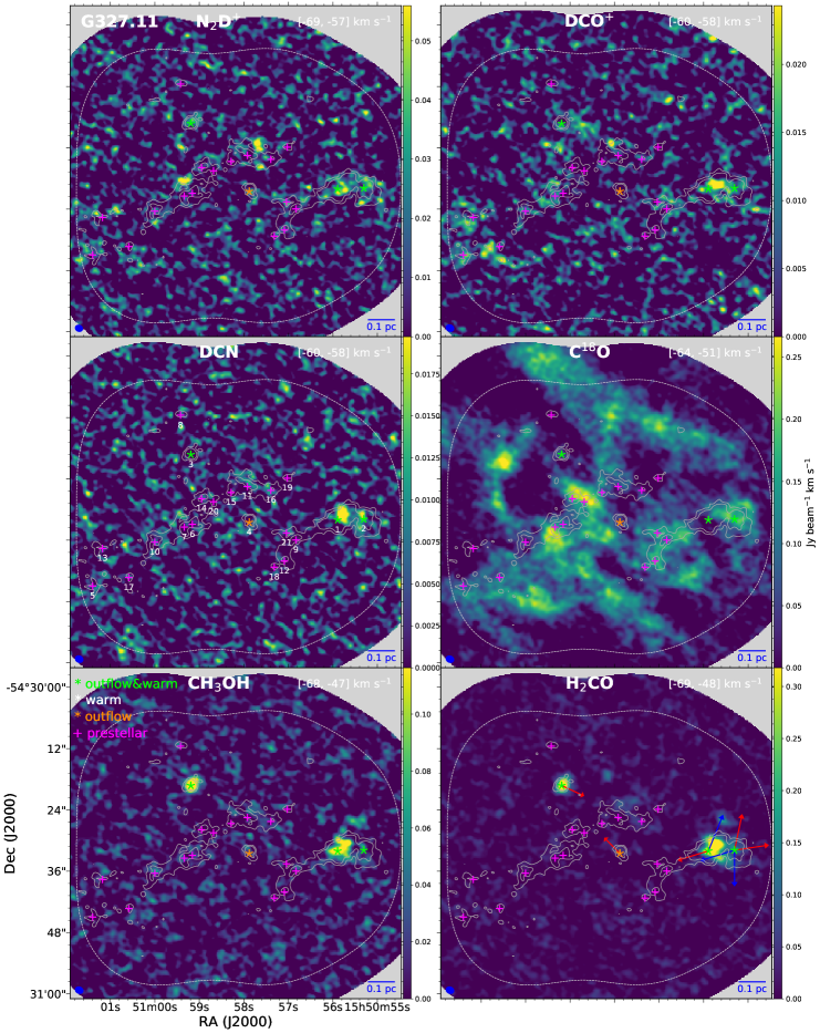
Figure 10:

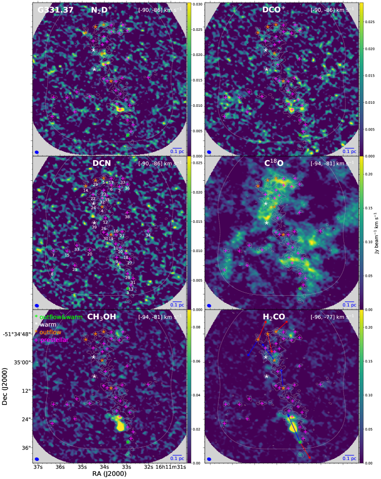
Figure 11: same as Figure 10, but for different sources.

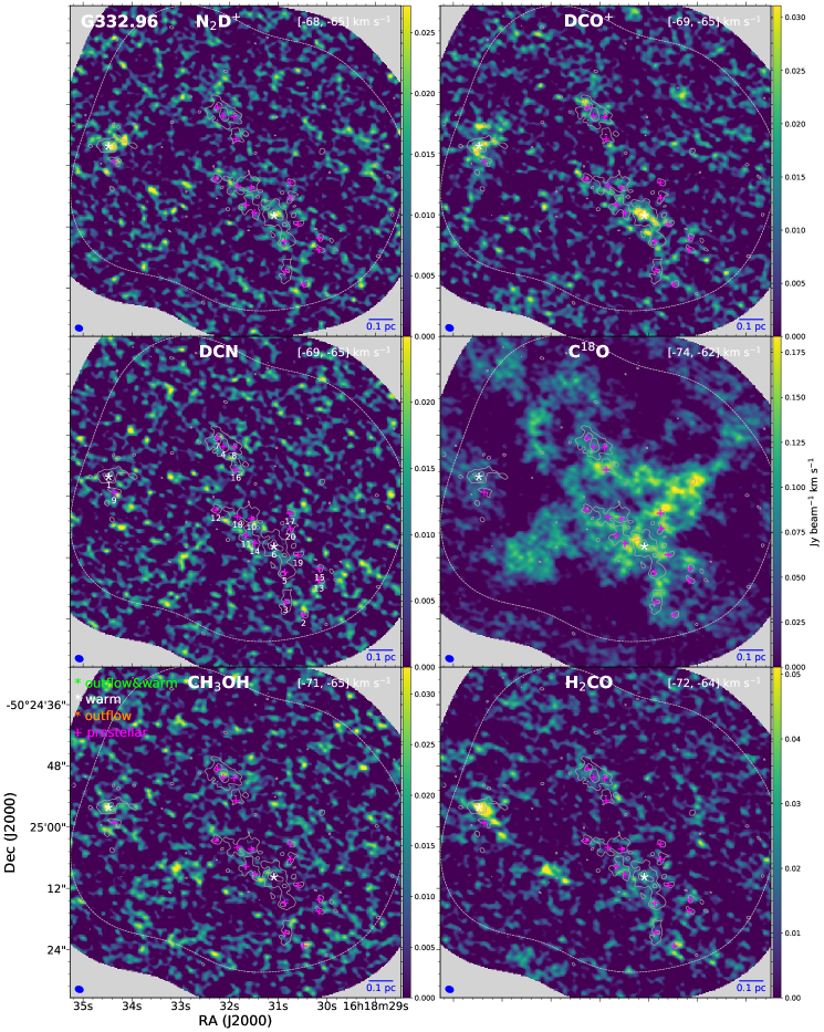
Figure 11:

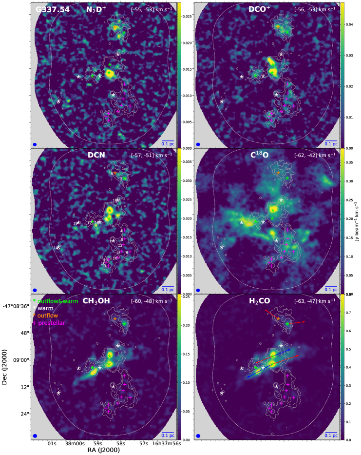
Figure 11:

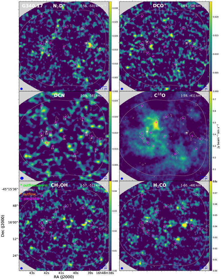
Figure 12: same as Figure 10, but for different sources.

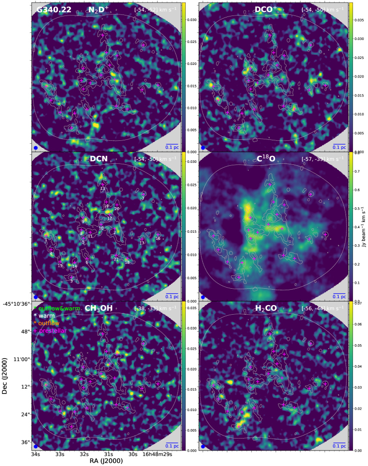
Figure 13: same as Figure 10, but for different sources.

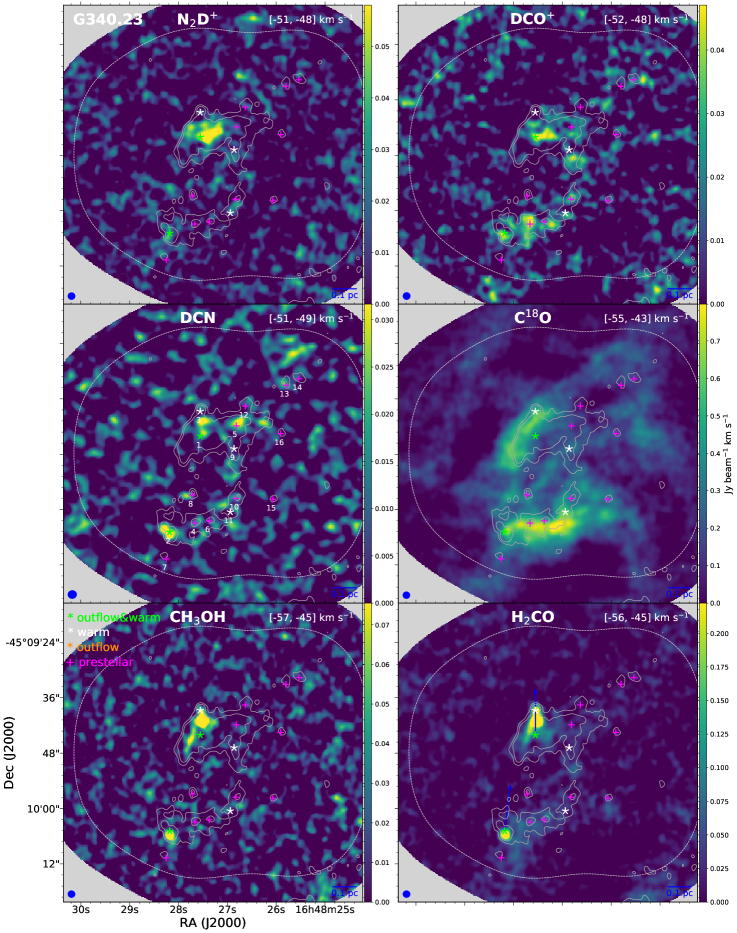
Figure 13:

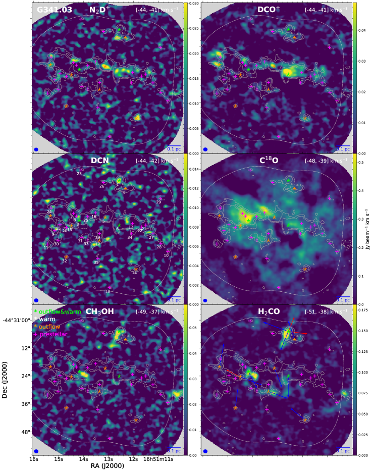
Figure 13:

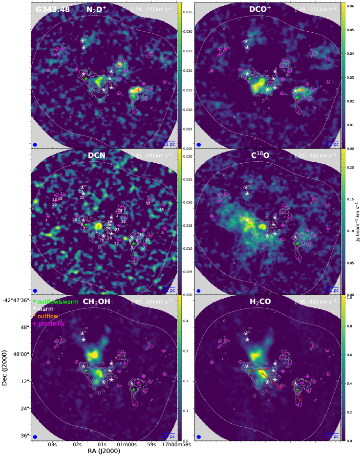
Figure 14: same as Figure 10, but for different sources.

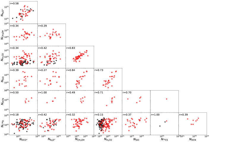
Figure 15: Column densities of each molecule plotted against one another. The black and red points represent the prestellar and protostellar cores, respectively.

Table 5: Summary of derived parameters of detected lines.

Molecule	core	$N_{\rm H_{2}}$	$n_{\rm H_{2}}$	$T_{\rm NH_{3}}$	$I_{\rm C^{18}O}$	$v_{\rm C^{18}O}$	$\sigma_{\rm C^{18}O}$	$N_{\rm C^{18}O}$	$I_{\rm DCO^{+}}$	$v_{\rm DCO^{+}}$	…
		$\times 10^{22}$ cm-2	$\times 10^{5}$ cm-3	K	K	km s-1	km s-1	$\times 10^{14}$ cm-2	K	km s-1	…
G10.99	1	4.78	1.59	13.4	0.69 (0.09)	0.69 (0.09)	30.16 (0.12)	0.76 (0.12)	0.41 (0.03)	29.75 (0.03)	…
G10.99	2	8.31	7.80	12.5	0.39 (0.08)	0.39 (0.08)	29.96 (0.13)	0.49 (0.11)	-	-	…
G10.99	3	7.80	5.21	11.7	0.65 (0.04)	0.65 (0.04)	29.92 (0.07)	1.07 (0.07)	0.51 (0.05)	29.63 (0.05)	…
G10.99	4	4.41	2.80	13.0	-	-	-	-	-	-	…
G10.99	5	5.55	2.33	13.3	0.62 (0.04)	0.62 (0.04)	29.28 (0.09)	1.12 (0.09)	0.79 (0.11)	29.90 (0.03)	…
G10.99	6	5.55	5.51	13.0	-	-	-	-	-	-	…
G10.99	7	5.29	2.15	12.3	1.23 (0.05)	1.23 (0.05)	29.62 (0.04)	0.85 (0.04)	1.74 (0.07)	29.56 (0.01)	…
G10.99	8	4.92	1.59	12.2	0.80 (0.04)	0.80 (0.04)	30.13 (0.04)	0.70 (0.04)	0.44 (0.06)	29.83 (0.05)	…
G10.99	9	4.25	2.43	13.3	0.84 (0.05)	0.84 (0.05)	29.38 (0.05)	0.74 (0.05)	0.66 (0.07)	29.52 (0.04)	…
G10.99	10	3.32	1.53	11.7	-	-	-	-	0.29 (0.05)	30.46 (0.05)	…
G10.99	11	5.56	6.16	11.4	0.33 (0.06)	0.33 (0.06)	30.74 (0.23)	1.10 (0.23)	0.87 (0.16)	29.78 (0.03)	…
G10.99	12	4.85	4.61	11.3	0.53 (0.09)	0.53 (0.09)	30.14 (0.11)	0.54 (0.11)	-	-	…
G10.99	13	3.21	1.55	13.0	0.80 (0.06)	0.80 (0.06)	28.99 (0.08)	0.96 (0.08)	-	-	…
G10.99	14	3.29	2.22	13.3	0.63 (0.07)	0.63 (0.07)	29.50 (0.13)	1.03 (0.13)	0.32 (0.06)	28.76 (0.08)	…
G10.99	15	3.38	1.66	13.3	1.10 (0.09)	1.10 (0.09)	29.54 (0.08)	0.91 (0.08)	-	-	…
…	…	…	…	…	…	…	…	…	…	…	…
G343.48	23	1.06	1.35	12.9	-	-	-	-	0.38 (0.06)	-28.62 (0.02)	…
G343.48	24	1.10	0.44	13.6	-	-	-	-	0.23 (0.04)	-28.93 (0.04)	…
G343.48	25	0.84	0.47	15.2	0.18 (0.02)	-28.25 (0.15)	0.92 (0.15)	2.32 (0.51)	-	-	…
G343.48	26	0.97	1.10	13.6	1.00 (0.03)	-28.84 (0.02)	0.60 (0.02)	8.78 (0.62)	-	-	…
G343.48	27	0.73	0.58	16.3	0.46 (0.03)	-28.73 (0.04)	0.40 (0.02)	2.63 (0.25)	-	-	…
G343.48	28	0.77	0.61	16.4	0.81 (0.03)	-28.40 (0.02)	0.52 (0.02)	6.05 (0.47)	0.33 (0.05)	-28.38 (0.03)	…
G343.48	29	1.05	0.62	12.0	0.11 (0.02)	-26.20 (0.17)	0.88 (0.17)	1.52 (0.40)	-	-	…

Appendix B Ammonia excitation temperature

Excitation temperatures were obtained using the method described in Mangum & Shirley (2015). The ammonia (1,1) and (2,2) transition spectra were modelled using five-component Gaussian models with seven parameters (systemic velocity, line width and five amplitude parameters, one for each hyperfine component). The best-fit model parameters were obtained using scipy’s “curve_fit” routine, using the TRF (“Trust Region Reflective”) algorithm.

From these parameters, the optical depth for the (1,1) transition, $\tau(1,1)$, was calculated from the ratio of the brightness of the satellite hyperfine transitions to the main component; this was solved numerically, using scipy’s “root” routine, using the Levenberg-Marquardt algorithm to minimise the sum of squares error of the four ratios simultaneously.

Finally, the brightness temperatures, $T_{\rm B}(1,1)$ and $T_{\rm B}(2,2)$, and the optical depth were combined with the line width parameter ($\Delta v(1,1)$ and $\Delta v(2,2)$, common to all hyperfine components) to calculate the excitation temperature, $T_{\rm NH_{3}}$, as

$$T_{\rm NH_{3}}=\frac{-41.5}{\ln\left[-\frac{0.283\Delta v(2,2)}{\tau(1,1)\Delta v(1,1)}\ln\left(1-\frac{T_{B}(2,2)}{T_{B}(1,1)}(1-\exp[-\tau(1,1)])\right)\right]}.$$ (B1)

Full details of this method for calculating optical depth and excitation temperature are given in Mangum & Shirley (2015).

The error bounds for the excitation temperature were then computed using a Monte Carlo approach. For each model parameter, a randomised value was repeatedly drawn (1000 times) from a Gaussian distribution with mean equal to the optimal parameter value and variance equal to the variance of the parameter estimates, as reported by the fitting routine. The optical depth and excitation temperature were then calculated using each set of randomised parameters, and the variance of the resulting distribution calculated to yield the temperature uncertainty.

Appendix C Column density

Assuming local thermodynamic equilibrium (LTE) and thin optical depths in the molecular line, the column densities of molecule can be calculated following (Mangum & Shirley, 2015)

$$N_{\rm mol}=\frac{3h}{8\pi^{3}R}\frac{Q_{\rm rot}}{S\mu^{2}g_{\rm u}}\frac{{\rm exp}(E_{\rm u}/kT_{\rm ex})}{{\rm exp}(h\nu/kT_{\rm ex})\,-\,1}\left(J_{\nu}(T_{\rm ex})\,-\,J_{\nu}(T_{\rm bg})\right)^{-1}\int\frac{T_{\rm B}dv}{f},$$ (C1)

where $h$ is the Planck constant, $S\mu^{2}$ is the line strength multiplied by the square of dipole moment, $R$ is the relative intensity of the main hyperfine transition with respect to the rest of hyperfine transitions, $g_{\rm u}$ is the statistical weight of the upper level, $T_{\rm ex}$ is the excitation temperature, $T_{\rm bg}$ is the back ground temperature, $E_{\rm u}$ is the energy of the upper state, $\nu$ is the transition frequency, $T_{\rm B}$ is brightness temperature, $\int T_{\rm B}dv$ is the velocity-integrated intensity, $f$ is the filling factor, and $Q_{\rm rot}$ is the partition function. Here $f$ is assumed to be 1 and $T_{\rm NH_{3}}$ approximates $T_{\rm ex}$ of molecular lines.

The molecular column density $N_{\rm H_{2}}$, gas mass $M_{\rm gas}$, and volume density $n_{\rm H_{2}}$ are derived from the continuum emission with

$$N_{\rm H_{2}}=\eta\frac{S_{\nu}}{B_{\nu}(T)\,\kappa_{\nu}\,\Omega\,\mu\,m_{\rm H}},$$ (C2)

$$M_{\rm gas}=\eta\frac{F_{\nu}\,\rm{D^{2}}}{\kappa_{\nu}\,B_{\nu}(T)},$$ (C3)

$$n_{\rm H_{2}}=\frac{M_{\rm gas}}{\frac{4}{3}\pi r^{3}\,\mu\,m_{\rm H}},$$ (C4)

where $\eta$=100 is the gas-to-dust ratio, $S_{\nu}$ is the peak flux density, $F_{\nu}$ is the measured integrated source flux, $\Omega$ is the beam solid angle, $m_{\rm H}$ is the mass of an hydrogen atom, $\mu$=2.8 is the mean molecular weight of the interstellar medium (Kauffmann et al., 2008), $\kappa_{\nu}$ is the dust opacity at a frequency of $\nu$, D is the distance to the source, and $r$ is the radius of dense cores. We adopted a value of 0.9 cm^-2 g^-1 for $\kappa_{\rm 1.3mm}$, which corresponds to the opacity of thin ice mantles and a gas density of 10⁶ cm^-3 (Ossenkopf & Henning, 1994).

The flux density is converted to brightness temperature following

$$T_{\rm B}=1.222\times 10^{3}\frac{I}{\nu^{2}\,\theta_{\rm maj}\,\theta_{\rm min}},$$ (C5)

where $T_{\rm B}$ is the brightness temperature in K, $I$ is the flux in mJy beam^-1, $\nu$ is the frequency in GHz, and $\theta_{\rm maj}$ and $\theta_{\rm min}$ are the half-power beam widths along the major and minor axes, respectively.

References

- Albertsson et al. (2013) Albertsson, T., Semenov, D. A., Vasyunin, A. I., Henning, T., & Herbst, E. 2013, ApJS, 207, 27, doi: 10.1088/0067-0049/207/2/27
- Arce et al. (2008) Arce, H. G., Santiago-García, J., Jørgensen, J. K., Tafalla, M., & Bachiller, R. 2008, ApJ, 681, L21, doi: 10.1086/590110
- Astropy Collaboration et al. (2013) Astropy Collaboration, Robitaille, T. P., Tollerud, E. J., et al. 2013, A&A, 558, A33, doi: 10.1051/0004-6361/201322068
- Barnes et al. (2016) Barnes, A. T., Kong, S., Tan, J. C., et al. 2016, MNRAS, 458, 1990, doi: 10.1093/mnras/stw403
- Bergin & Tafalla (2007) Bergin, E. A., & Tafalla, M. 2007, ARA&A, 45, 339, doi: 10.1146/annurev.astro.45.071206.100404
- Bernstein et al. (2002) Bernstein, M. P., Dworkin, J. P., Sandford, S. A., Cooper, G. W., & Allamandola, L. J. 2002, Nature, 416, 401, doi: 10.1038/416401a
- Bisschop et al. (2007) Bisschop, S. E., Jørgensen, J. K., van Dishoeck, E. F., & de Wachter, E. B. M. 2007, A&A, 465, 913, doi: 10.1051/0004-6361:20065963
- Booth et al. (2021) Booth, A. S., Walsh, C., Terwisscha van Scheltinga, J., et al. 2021, Nature Astronomy, 5, 684, doi: 10.1038/s41550-021-01352-w
- Caselli & Ceccarelli (2012) Caselli, P., & Ceccarelli, C. 2012, A&A Rev., 20, 56, doi: 10.1007/s00159-012-0056-x
- Caselli et al. (2002) Caselli, P., Walmsley, C. M., Zucconi, A., et al. 2002, ApJ, 565, 344, doi: 10.1086/324302
- Charnley et al. (1997) Charnley, S. B., Tielens, A. G. G. M., & Rodgers, S. D. 1997, ApJ, 482, L203, doi: 10.1086/310697
- Chen et al. (2010) Chen, H.-R., Liu, S.-Y., Su, Y.-N., & Zhang, Q. 2010, ApJ, 713, L50, doi: 10.1088/2041-8205/713/1/L50
- Cohen (1988) Cohen, J. 1988, 1988 Statistical Power Analysis for the Behavioral Sciences (Hillsdale, NJ: L. Erlbaum Associates)
- Contreras et al. (2018) Contreras, Y., Sanhueza, P., Jackson, J. M., et al. 2018, ApJ, 861, 14, doi: 10.3847/1538-4357/aac2ec
- Dalgarno & Lepp (1984) Dalgarno, A., & Lepp, S. 1984, ApJ, 287, L47, doi: 10.1086/184395
- Drozdovskaya et al. (2019) Drozdovskaya, M. N., van Dishoeck, E. F., Rubin, M., Jørgensen, J. K., & Altwegg, K. 2019, MNRAS, 490, 50, doi: 10.1093/mnras/stz2430
- Feng et al. (2020) Feng, S., Li, D., Caselli, P., et al. 2020, ApJ, 901, 145, doi: 10.3847/1538-4357/abada3
- Fuchs et al. (2009) Fuchs, G. W., Cuppen, H. M., Ioppolo, S., et al. 2009, A&A, 505, 629, doi: 10.1051/0004-6361/200810784
- Garrod et al. (2006) Garrod, R., Park, I. H., Caselli, P., & Herbst, E. 2006, Faraday Discussions, 133, 51, doi: 10.1039/b516202e
- Garrod et al. (2008) Garrod, R. T., Widicus Weaver, S. L., & Herbst, E. 2008, ApJ, 682, 283, doi: 10.1086/588035
- Gerner et al. (2014) Gerner, T., Beuther, H., Semenov, D., et al. 2014, A&A, 563, A97, doi: 10.1051/0004-6361/201322541
- Gerner et al. (2015) Gerner, T., Shirley, Y. L., Beuther, H., et al. 2015, A&A, 579, A80, doi: 10.1051/0004-6361/201423989
- Giannetti et al. (2019) Giannetti, A., Bovino, S., Caselli, P., et al. 2019, A&A, 621, L7, doi: 10.1051/0004-6361/201834602
- Ginsburg et al. (2022) Ginsburg, A., Sokolov, V., de Val-Borro, M., et al. 2022, AJ, 163, 291, doi: 10.3847/1538-3881/ac695a
- Guzmán et al. (2018) Guzmán, A. E., Guzmán, V. V., Garay, G., Bronfman, L., & Hechenleitner, F. 2018, ApJS, 236, 45, doi: 10.3847/1538-4365/aac01d
- Guzmán et al. (2013) Guzmán, V. V., Goicoechea, J. R., Pety, J., et al. 2013, A&A, 560, A73, doi: 10.1051/0004-6361/201322460
- Herbst & van Dishoeck (2009) Herbst, E., & van Dishoeck, E. F. 2009, ARA&A, 47, 427, doi: 10.1146/annurev-astro-082708-101654
- Hoq et al. (2013) Hoq, S., Jackson, J. M., Foster, J. B., et al. 2013, ApJ, 777, 157, doi: 10.1088/0004-637X/777/2/157
- Hunter (2007) Hunter, J. D. 2007, Computing in Science Engineering, 9, 90
- Immer et al. (2014) Immer, K., Galván-Madrid, R., König, C., Liu, H. B., & Menten, K. M. 2014, A&A, 572, A63, doi: 10.1051/0004-6361/201423780
- Jørgensen et al. (2020) Jørgensen, J. K., Belloche, A., & Garrod, R. T. 2020, ARA&A, 58, 727, doi: 10.1146/annurev-astro-032620-021927
- Jørgensen et al. (2005) Jørgensen, J. K., Schöier, F. L., & van Dishoeck, E. F. 2005, A&A, 437, 501, doi: 10.1051/0004-6361:20042060
- Kauffmann et al. (2008) Kauffmann, J., Bertoldi, F., Bourke, T. L., Evans, N. J., I., & Lee, C. W. 2008, A&A, 487, 993, doi: 10.1051/0004-6361:200809481
- Kong et al. (2017) Kong, S., Tan, J. C., Caselli, P., et al. 2017, ApJ, 834, 193, doi: 10.3847/1538-4357/834/2/193
- Le Teuff et al. (2000) Le Teuff, Y. H., Millar, T. J., & Markwick, A. J. 2000, A&AS, 146, 157, doi: 10.1051/aas:2000265
- Leurini et al. (2010) Leurini, S., Parise, B., Schilke, P., Pety, J., & Rolffs, R. 2010, A&A, 511, A82, doi: 10.1051/0004-6361/200912484
- Li et al. (2017) Li, S., Wang, J., Zhang, Z.-Y., et al. 2017, MNRAS, 466, 248, doi: 10.1093/mnras/stw3076
- Li et al. (2019) Li, S., Wang, J., Fang, M., et al. 2019, ApJ, 878, 29, doi: 10.3847/1538-4357/ab1e4c
- Li et al. (2020) Li, S., Sanhueza, P., Zhang, Q., et al. 2020, ApJ, 903, 119, doi: 10.3847/1538-4357/abb81f
- Li et al. (2021) Li, S., Lu, X., Zhang, Q., et al. 2021, ApJ, 912, L7, doi: 10.3847/2041-8213/abf64f
- Liu et al. (2020) Liu, H.-L., Sanhueza, P., Liu, T., et al. 2020, ApJ, 901, 31, doi: 10.3847/1538-4357/abadfe
- Lu et al. (2021) Lu, X., Li, S., Ginsburg, A., et al. 2021, ApJ, 909, 177, doi: 10.3847/1538-4357/abde3c
- Mangum & Shirley (2015) Mangum, J. G., & Shirley, Y. L. 2015, PASP, 127, 266, doi: 10.1086/680323
- Maret et al. (2005) Maret, S., Ceccarelli, C., Tielens, A. G. G. M., et al. 2005, A&A, 442, 527, doi: 10.1051/0004-6361:20052899
- Maret et al. (2004) Maret, S., Ceccarelli, C., Caux, E., et al. 2004, A&A, 416, 577, doi: 10.1051/0004-6361:20034157
- McMullin et al. (2007) McMullin, J. P., Waters, B., Schiebel, D., Young, W., & Golap, K. 2007, in Astronomical Society of the Pacific Conference Series, Vol. 376, Astronomical Data Analysis Software and Systems XVI, ed. R. A. Shaw, F. Hill, & D. J. Bell, 127
- Miettinen (2014) Miettinen, O. 2014, A&A, 562, A3, doi: 10.1051/0004-6361/201322596
- Morii et al. (2021) Morii, K., Sanhueza, P., Nakamura, F., et al. 2021, ApJ, 923, 147, doi: 10.3847/1538-4357/ac2365
- Mottram et al. (2020) Mottram, J. C., Beuther, H., Ahmadi, A., et al. 2020, A&A, 636, A118, doi: 10.1051/0004-6361/201834152
- Muñoz Caro et al. (2002) Muñoz Caro, G. M., Meierhenrich, U. J., Schutte, W. A., et al. 2002, Nature, 416, 403, doi: 10.1038/416403a
- Müller et al. (2005) Müller, H. S. P., Schlöder, F., Stutzki, J., & Winnewisser, G. 2005, Journal of Molecular Structure, 742, 215, doi: 10.1016/j.molstruc.2005.01.027
- Öberg & Bergin (2021) Öberg, K. I., & Bergin, E. A. 2021, Phys. Rep., 893, 1, doi: 10.1016/j.physrep.2020.09.004
- Ossenkopf & Henning (1994) Ossenkopf, V., & Henning, T. 1994, A&A, 291, 943
- Pagani et al. (2007) Pagani, L., Bacmann, A., Cabrit, S., & Vastel, C. 2007, A&A, 467, 179, doi: 10.1051/0004-6361:20066670
- Pagani et al. (2009) Pagani, L., Vastel, C., Hugo, E., et al. 2009, A&A, 494, 623, doi: 10.1051/0004-6361:200810587
- Peng et al. (2022) Peng, Y., Liu, T., Qin, S.-L., et al. 2022, MNRAS, 512, 4419, doi: 10.1093/mnras/stac624
- Pineda et al. (2022) Pineda, J. E., Harju, J., Caselli, P., et al. 2022, AJ, 163, 294, doi: 10.3847/1538-3881/ac6be7
- Qin et al. (2022) Qin, S.-L., Liu, T., Liu, X., et al. 2022, MNRAS, 511, 3463, doi: 10.1093/mnras/stac219
- Redaelli et al. (2019) Redaelli, E., Bizzocchi, L., Caselli, P., et al. 2019, A&A, 629, A15, doi: 10.1051/0004-6361/201935314
- Redaelli et al. (2021) Redaelli, E., Bovino, S., Giannetti, A., et al. 2021, A&A, 650, A202, doi: 10.1051/0004-6361/202140694
- Requena-Torres et al. (2006) Requena-Torres, M. A., Martín-Pintado, J., Rodríguez-Franco, A., et al. 2006, A&A, 455, 971, doi: 10.1051/0004-6361:20065190
- Robitaille & Bressert (2012) Robitaille, T., & Bressert, E. 2012, APLpy: Astronomical Plotting Library in Python, Astrophysics Source Code Library. http://ascl.net/1208.017
- Rosolowsky et al. (2008) Rosolowsky, E. W., Pineda, J. E., Kauffmann, J., & Goodman, A. A. 2008, ApJ, 679, 1338, doi: 10.1086/587685
- Sabatini et al. (2019) Sabatini, G., Giannetti, A., Bovino, S., et al. 2019, MNRAS, 490, 4489, doi: 10.1093/mnras/stz2818
- Sabatini et al. (2020) Sabatini, G., Bovino, S., Giannetti, A., et al. 2020, A&A, 644, A34, doi: 10.1051/0004-6361/202039010
- Sabatini et al. (2021) —. 2021, A&A, 652, A71, doi: 10.1051/0004-6361/202140469
- Sabatini et al. (2022) Sabatini, G., Bovino, S., Sanhueza, P., et al. 2022, arXiv e-prints, arXiv:2207.12431. https://arxiv.org/abs/2207.12431
- Sakai et al. (2012) Sakai, N., Ceccarelli, C., Bottinelli, S., Sakai, T., & Yamamoto, S. 2012, ApJ, 754, 70, doi: 10.1088/0004-637X/754/1/70
- Sakai et al. (2022) Sakai, T., Sanhueza, P., Furuya, K., et al. 2022, ApJ, 925, 144, doi: 10.3847/1538-4357/ac3d2e
- Sanhueza et al. (2010) Sanhueza, P., Garay, G., Bronfman, L., et al. 2010, ApJ, 715, 18, doi: 10.1088/0004-637X/715/1/18
- Sanhueza et al. (2012) Sanhueza, P., Jackson, J. M., Foster, J. B., et al. 2012, ApJ, 756, 60, doi: 10.1088/0004-637X/756/1/60
- Sanhueza et al. (2013) —. 2013, ApJ, 773, 123, doi: 10.1088/0004-637X/773/2/123
- Sanhueza et al. (2017) Sanhueza, P., Jackson, J. M., Zhang, Q., et al. 2017, ApJ, 841, 97, doi: 10.3847/1538-4357/aa6ff8
- Sanhueza et al. (2019) Sanhueza, P., Contreras, Y., Wu, B., et al. 2019, ApJ, 886, 102, doi: 10.3847/1538-4357/ab45e9
- Schöier et al. (2005) Schöier, F. L., van der Tak, F. F. S., van Dishoeck, E. F., & Black, J. H. 2005, A&A, 432, 369, doi: 10.1051/0004-6361:20041729
- Tafalla et al. (2010) Tafalla, M., Santiago-García, J., Hacar, A., & Bachiller, R. 2010, A&A, 522, A91, doi: 10.1051/0004-6361/201015158
- Tafalla et al. (2006) Tafalla, M., Santiago-García, J., Myers, P. C., et al. 2006, A&A, 455, 577, doi: 10.1051/0004-6361:20065311
- Tafoya et al. (2021) Tafoya, D., Sanhueza, P., Zhang, Q., et al. 2021, ApJ, 913, 131, doi: 10.3847/1538-4357/abf5da
- Turner (2001) Turner, B. E. 2001, ApJS, 136, 579, doi: 10.1086/322536
- Tychoniec et al. (2021) Tychoniec, Ł., van Dishoeck, E. F., van’t Hoff, M. L. R., et al. 2021, A&A, 655, A65, doi: 10.1051/0004-6361/202140692
- van Dishoeck & Blake (1998) van Dishoeck, E. F., & Blake, G. A. 1998, ARA&A, 36, 317, doi: 10.1146/annurev.astro.36.1.317
- Vasyunina et al. (2014) Vasyunina, T., Vasyunin, A. I., Herbst, E., et al. 2014, ApJ, 780, 85, doi: 10.1088/0004-637X/780/1/85
- Watanabe et al. (2004) Watanabe, N., Nagaoka, A., Shiraki, T., & Kouchi, A. 2004, ApJ, 616, 638, doi: 10.1086/424815
- Wootten & Loren (1987) Wootten, A., & Loren, R. B. 1987, ApJ, 317, 220, doi: 10.1086/165270