Fondue: an algorithm to find the optimal dimensionality of the latent representations of variational autoencoders

Abstract

When training a variational autoencoder (VAE) on a given dataset, determining the optimal number of latent variables is mostly done by grid search — a costly process in terms of computational time and carbon footprint. In this paper, we explore the intrinsic dimension estimation (IDE) of the data and latent representations learned by VAEs. We show that the discrepancies between the IDE of the mean and sampled representations of a VAE after only a few steps of training reveal the presence of passive variables in the latent space, which, in well-behaved VAEs, indicates a superfluous number of dimensions. Using this property, we propose FONDUE: an algorithm which quickly finds the number of latent dimensions after which the mean and sampled representations start to diverge (i.e., when passive variables are introduced), providing a principled method for selecting the number of latent dimensions for VAEs and autoencoders.

1 Introduction

“How many latent variables should I use for this model?” is a question that many practitioners using variational autoencoders (VAEs) or autoencoders (AEs) have to deal with. When the task has been studied before, this information is available in the literature for the specific architecture and dataset used. However, when it has not, answering this question becomes more complicated. Indeed, the dimensionality of the latent representation is usually determined empirically by increasing the number of latent dimensions until the reconstruction does not improve anymore (Doersch, 2016). This is a costly process requiring multiple model training, and increasing the carbon footprint and time needed for an experiment.

In recent years, topology-based methods have successfully been applied to deep learning (Hensel et al., 2021) and generative models to design new metrics (Khrulkov & Oseledets, 2018; Zhou et al., 2021; Rieck et al., 2019) and learning methods (Falorsi et al., 2018; Perez Rey et al., 2020; Keller & Welling, 2021). They have also been used to analyse the representations learned by deep neural networks (DNNs) (Arvanitidis et al., 2018; Ansuini et al., 2019; Maheswaranathan et al., 2019; Naitzat et al., 2020).

Intrinsic dimension estimation (IDE) — the estimation of the minimum number of variables needed to describe the data — is an active area of reseach in topology, and various estimation methods have been proposed (Facco et al., 2017; Levina & Bickel, 2004). Using these techniques, the intrinsic dimension (ID) of images was empirically shown to be much lower than their extrinsic dimension (i.e., the number of pixels) (Gong et al., 2019; Ansuini et al., 2019; Pope et al., 2021). Moreover, Ansuini et al. (2019) observed that the ID of neural network classifiers with good generalisation tended to first increase, then decrease until reaching a very low ID in the last layer.

As IDE provides an estimate of the minimum number of variables needed to describe the data, it could be an invaluable tool to determine the number of latent variables needed for VAEs and avoid costly grid searches, effectively reducing the carbon footprint of model implementations.

Thus, our objective in this paper is to verify whether the ID of different layers can be used to determine the number of latent variables in VAEs.

Our contributions are as follows:

1. We provide an experimental study of the IDE of VAEs, and have released more than 35,000 IDE scores (https://data.kent.ac.uk/id/eprint/455).

2. We have released the library created for this experiment (https://github.com/bonheml/VAE_learning_dynamics). It can be reused with other IDE techniques or models for further research in the domain.

3. During our analysis of VAEs, we found that (1) the deeper the layer of the encoder, the lower the estimated IDs, whereas the layers of the decoder all have the same IDE; (2) the extrinsic dimensionality of the latent representations is generally higher than its IDE; (3) the layers reach a stable ID very early in the training; and (4) the IDE of mean and sampled representations is different when some latent variables collapse.

4. Based on these findings, we propose FONDUE: an algorithm for Finding the Optimal Number of Dimensions by Unsupervised Estimation, which works well on the three datasets used in our experiment.

2 Background

2.1 Variational Autoencoders

VAEs (Kingma & Welling, 2014; Rezende & Mohamed, 2015) are deep probabilistic generative models based on variational inference. The encoder maps an input ${\mathbf{x}}$ to a latent representation ${\mathbf{z}}$, and the decoder attempts to reconstruct ${\mathbf{x}}$ using ${\mathbf{z}}$. This can be optimised by maximising $\mathcal{L}$, the evidence lower bound (ELBO)

$$\operatorname{\mathcal{L}({\bm{\theta}},{\bm{\phi}};{\mathbf{x}})}=\underbrace{\mathbb{E}_{q_{\bm{\phi}}({\mathbf{z}}|{\mathbf{x}})}[\log p_{\bm{\theta}}({\mathbf{x}}|{\mathbf{z}})]}_{\text{reconstruction term}}-\underbrace{D_{\mathrm{KL}}\left(q_{\bm{\phi}}({\mathbf{z}}|{\mathbf{x}})||p({\mathbf{z}})\right)}_{\text{regularisation term}},$$ (1)

where $p({\mathbf{z}})$ is generally modelled as a standard multivariate Gaussian distribution $\mathcal{N}(0,{\bm{I}})$ to permit a closed form computation of the regularisation term (Doersch, 2016). The regularisation term can be further penalised by a weight $\beta$ (Higgins et al., 2017) such that

$$\operatorname{\mathcal{L}({\bm{\theta}},{\bm{\phi}};{\mathbf{x}})}=\underbrace{\mathbb{E}_{q_{\bm{\phi}}({\mathbf{z}}|{\mathbf{x}})}[\log p_{\bm{\theta}}({\mathbf{x}}|{\mathbf{z}})]}_{\text{reconstruction term}}-\underbrace{\beta D_{\mathrm{KL}}\left(q_{\bm{\phi}}({\mathbf{z}}|{\mathbf{x}})||p({\mathbf{z}})\right)}_{\text{regularisation term}},$$ (2)

reducing to equation 1 when $\beta=1$ and to a deterministic auto-encoder when $\beta=0$.

Posterior collapse and polarised regime

When $\beta\geqslant 1$, VAEs can produce disentangled representations (Higgins et al., 2017) but too high values of $\beta$ result in posterior collapse (i.e., ${\mathbf{z}}\sim\mathcal{N}(0,{\bm{I}})$) making the model unusable (Lucas et al., 2019a; b; Dai et al., 2020). Indeed, the sampled representation will not retain any information from the input, making it impossible for the decoder to correctly reconstruct the image. Nevertheless, for VAEs to provide good reconstruction (Dai & Wipf, 2018; Dai et al., 2020), it is necessary for any superfluous dimensions of ${\mathbf{z}}$ to be collapsed and ignored by the decoder. These collapsed dimensions are called passive variables; the remaining, active variables. When this selective posterior collapse behaviour — also known as the polarised regime (Rolinek et al., 2019) — happens, the passive variables are very different in mean and sampled representations (Bonheme & Grzes, 2021) (see also Appendices E and F).

2.2 Intrinsic dimension estimation

It is generally assumed that a dataset ${\bm{X}}$ of $m$ i.i.d. data examples ${\bm{X}}_{i}\in\mathbb{R}^{n}$ is a locally smooth non-linear transformation $g$ of a lower-dimensional dataset ${\bm{Y}}$ of $m$ i.i.d. samples ${\bm{Y}}_{i}\in\mathbb{R}^{d}$, where $d\leqslant n$ (Campadelli et al., 2015; Chollet, 2021). The goal of intrinsic dimension estimation (IDE) is to recover $d$ given ${\bm{X}}$. In this section, we will detail two IDE techniques which use the statistical properties of the neighbourhood of each data point to estimate $d$, and provide good results for approximating the ID of deep neural network representations and deep learning datasets (Ansuini et al., 2019; Gong et al., 2019; Pope et al., 2021).

Maximum Likelihood Estimation

Levina & Bickel (2004) modelled the neighbourhood of a given point ${\bm{X}}_{i}$ as a Poisson process in a d-dimensional sphere $S_{{\bm{X}}_{i}}(R)$ of radius $R$ around ${\bm{X}}_{i}$. This Poisson process is denoted $\{N(t,{\bm{X}}_{i}),0\leqslant t\leqslant R\}$, where $N(t,{\bm{X}}_{i})$ is a random variable (distributed according to a Poisson distribution) representing the number of neighbours of ${\bm{X}}_{i}$ within a radius $t$. Each point ${\bm{X}}_{j}\in S_{{\bm{X}}_{i}}(R)$ is thus considered as an event, its arrival time $t=T({\bm{X}}_{i},{\bm{X}}_{j})$ being the Euclidean distance from ${\bm{X}}_{i}$ to its $j^{th}$ neighbour ${\bm{X}}_{j}$. By expressing the rate $\lambda(t,{\bm{X}}_{i})$ of the process $N(t,{\bm{X}}_{i})$ as a function of the surface area of the sphere — and thus relating $\lambda(t,{\bm{X}}_{i})$ to $d$ — they obtain a maximum likelihood estimation (MLE) of the intrinsic dimension $d$:

$$\bar{d}_{R}({\bm{X}}_{i})=\left[\frac{1}{N(R,{\bm{X}}_{i})}\sum_{j=1}^{N(R,{\bm{X}}_{i})}\log\frac{R}{T({\bm{X}}_{i},{\bm{X}}_{j})}\right]^{-1}.$$ (3)

Equation 3 is then simplified by fixing the number of neighbours, $k$, instead of the radius $R$ of the sphere, such that

$$\bar{d}_{k}({\bm{X}}_{i})=\left[\frac{1}{k-1}\sum_{j=1}^{k-1}\log\frac{T({\bm{X}}_{i},{\bm{X}}_{k})}{T({\bm{X}}_{i},{\bm{X}}_{j})}\right]^{-1},$$ (4)

where the last summand is omitted, as it is zero for $j=k$. The final estimate $\bar{d}_{k}$ is the averaged score over $n$ data examples (Levina & Bickel, 2004)

$$\bar{d}_{k}=\frac{1}{n}\sum_{i=1}^{n}\bar{d}_{k}({\bm{X}}_{i}).$$ (5)

To obtain an accurate estimation of the ID with MLE, it is very important to choose a sufficient number of neighbours $k$ to form a dense small sphere (Levina & Bickel, 2004). On one hand, if $k$ is too small, MLE will generally underestimate the ID, and suffer from high variance (Levina & Bickel, 2004; Campadelli et al., 2015; Pope et al., 2021). On the other hand, if $k$ is too large, the ID will be overestimated (Levina & Bickel, 2004; Pope et al., 2021).

TwoNN

Facco et al. (2017) proposed an estimation of the ID based on the ratio of the two nearest neighbours of ${\bm{X}}_{i}$, $r_{{\bm{X}}_{i}}=\frac{T({\bm{X}}_{i},{\bm{X}}_{l})}{T({\bm{X}}_{i},{\bm{X}}_{j})}$, where ${\bm{X}}_{j}$ and ${\bm{X}}_{l}$ are the first and second closest neighbours of ${\bm{X}}_{i}$, respectively. $r$ follows a Pareto distribution with scale $s=1$ and shape $d$, and its density function $f(r)$ is

$$f(r)=\frac{ds^{d}}{r^{d+1}}=dr^{-(d+1)}.$$ (6)

Its cumulative distribution function is thus

$$F(r)=1-\frac{s^{d}}{r^{d}}=1-r^{-d},$$ (7)

and, using Equation 7, one can readily obtain $d=\frac{-\log(1-F(r))}{\log{r}}$. From this, we can see that $d$ is the slope of the straight line passing through the origin, which is given by the set of coordinates ${\mathbb{S}}=\{(\>\log r_{{\bm{X}}_{i}},-\log(1-F(r_{{\bm{X}}_{i}}))\>)\;|\;i=1,\cdots,m\}$, and can be recovered by linear regression.

As TwoNN uses only two neighbours, it can be sensitive to outliers (Facco et al., 2017) and do not perform well on high ID (Pope et al., 2021), overestimating the ID in both cases.

Ensuring an accurate analysis

Given the limitations previously mentioned, we take two remedial actions to guarantee that our analysis is as accurate as possible. To provide an IDE which is as accurate as possible with MLE, we will measure the MLE with an increasing number of neighbours and, similar to Karbauskaitė et al. (2011), retain the IDE which is stable for the largest number of $k$ values. TwoNN will be used as a complementary metric to validate our choice of $k$ for MLE. In case of significant discrepancies with a significantly higher TwoNN IDE, we will rely on the results provided by MLE.

3 Experimental setup

As mentioned in section 1, the main objective of our experiment is to investigate the IDs of the representations learned by VAEs to assess whether they can be used to determine the optimal number of latent dimensions of VAEs.

To do so, we will train VAEs with at least 8 different numbers of latent dimensions on 3 datasets of increasing ID and estimate the ID of each layer of the models. We will then analyse these results and use them to verify our objectives in Section 4.

Datasets

We use three datasets with an increasing number of intrinsic dimensions: Symmetric solids (Murphy et al., 2021), dSprites (Higgins et al., 2017), and Celeba (Liu et al., 2015). The numbers of generative factors of the first two datasets are 2 and 5, respectively, and the IDE of these two datasets should be close to these values. While we do not know the generative factors of Celeba, Pope et al. (2021) reported an IDE greater than 20, which is high enough for our experiment.

Data preprocessing

Each image is resized to $64\times 64\times c$, where $c=1$ for Symmetric solids and dSprites, and $c=3$ for Celeba. We also removed duplicate images (i.e., cases where different rotations resulted in the same image) and labels from Symmetric solids and created a reduced version: symsol_reduced which is available  at https://data.kent.ac.uk/436.

VAE training

We use the $\beta$-VAE architecture detailed in Higgins et al. (2017) for all the datasets, together with the standard learning objective of VAEs, as presented in Equation 1. Each VAE is trained 5 times with a number of latent dimensions $n=3,6,8,10,12,18,24,32$ on every dataset. For Celeba, which has the highest IDE, we additionally train VAEs with latent dimensions $n=42,52,62,100,150,200$.

Estimations of the ID

For all the models, we estimate the ID of the layers’ activations using 3 batches of 10,000 data examples each. As in Pope et al. (2021), the MLE scores are computed with $k=3,5,10,20$.

Additional details on our implementation can be found in Appendix C and our code is available at https://github.com/bonheml/VAE_learning_dynamics.

4 Results

In this section, we will analyse the results of the experiment detailed in Section 3. First, we will review the IDE of the different datasets in Section 4.1. Then, in Section 4.2, we will discuss the variation of IDs between different layers of VAEs when we change the number of latent dimensions and how it evolves during training. Finally, based on the findings of these sections, we will answer the objective of Section 3 by proposing FONDUE — an algorithm to automatically find the optimal number of latent dimensions for VAEs in an efficient and unsupervised way — in Section 4.3.

4.1 Estimating the intrinsic dimensions of the datasets

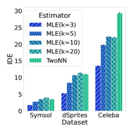
Figure 1: Intrinsic dimension estimation of dSprites, Celeba, and Symsol using different ID estimators. We can see that MLE have very close estimates for 10 and 20 neighbours, which generally agree with TwoNN estimates. However, TwoNN seems to overestimate the ID of Celeba.

Following Karbauskaitė et al. (2011), we will retain for our analysis the MLE estimates which are stable for the largest number of $k$ values, as detailed in Section 2.2. We can see in Figure 1 that the MLE estimations become stable when $k$ is between 10 and 20, similar to what was reported by Levina & Bickel (2004). These IDEs are also generally close to TwoNN estimations, except for Celeba, where TwoNN seems to overestimate the ID, as previously reported by Pope et al. (2021). In the rest of this paper, we will thus consider the IDEs obtained from MLE with $k=20$ as our most likely IDEs.

As mentioned in Section 3, we have selected 3 datasets of increasing intrinsic dimensionality: Symsol (Murphy et al., 2021), dSprites (Higgins et al., 2017), and Celeba (Liu et al., 2015). Celeba’s IDE was previously estimated to be 26 for MLE with $k=20$ (Pope et al., 2021), and we know that Symsol and dSprites have 2 and 5 generative factors, respectively. We thus expect their IDEs to be close to these values.  We can see in Figure 1 that MLE and TwoNN overestimate the IDs of Symsol and dSprites, with IDEs of 4 and 11 instead of the expected 2 and 5. Our result for Celeba is close to Pope et al. (2021) with an estimate of 22; the slight difference may be attributed to the difference in our averaging process (Pope et al. (2021) used the averaging described by MacKay & Ghahramani (2005) instead of the original averaging of Levina & Bickel (2004) given in Equation 5).

Overall, we can see that we get an upper bound on the true ID of the data for the datasets whose ID are known. However, as we will study the variations of ID over different layers, our experiment will not be impacted by any overestimation of the true ID.

4.2 Analysing the IDE of the different layers of VAEs

Now that we have an IDE for each of the datasets, we are interested in observing how the ID of VAEs varies between layers and when they are trained with different numbers of latent variables.

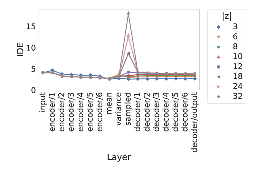
(a) Symsol

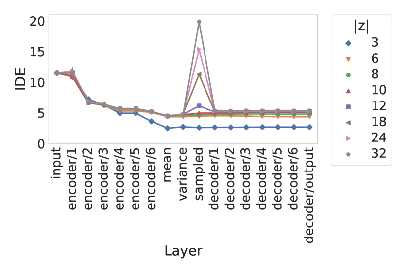
(b) dSprites

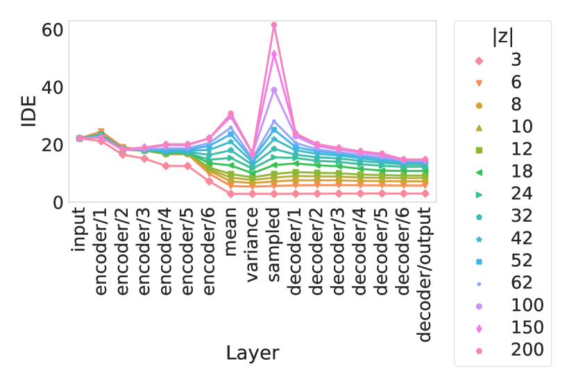
(c) Celeba

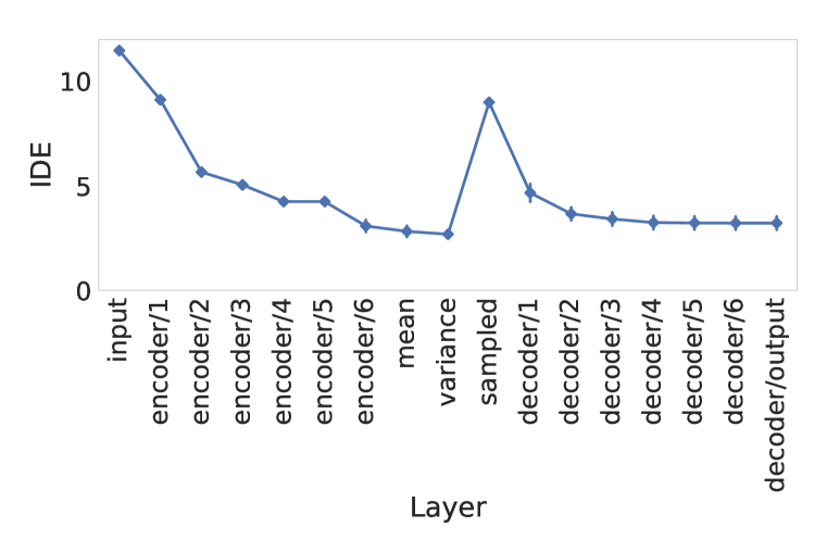
(d) $\beta$-VAE trained on dSprites with 10 latent variables and $\beta=20$.

Figure 2: Intrinsic dimension estimation of VAEs trained with an increasing number of latent dimensions $|{\mathbf{z}}|$. (a), (b), and (c) show the results on Symsol, dSprites, and Celeba, respectively. (d) shows the results of $\beta$-VAEs trained on dSprites with 10 latent variables and $\beta=20$ to cause posterior collapse.

The ID of the encoder decreases, but the ID of the decoder stays constant

We can see in Figure 2 that the ID of the representations learned by the encoder decreases until we reach the mean and variance layers, which is consistent with the observations reported for classification (Ansuini et al., 2019). Interestingly, for dSprites and Symsol, when the number of latent variables is at least equal to the ID of the data, the IDE of the mean and variance representations is very close to the true data ID. After a local increase of the ID in the sampled representations, the ID of the decoder representations stays close to the ID of the mean representations and does not change much between layers.

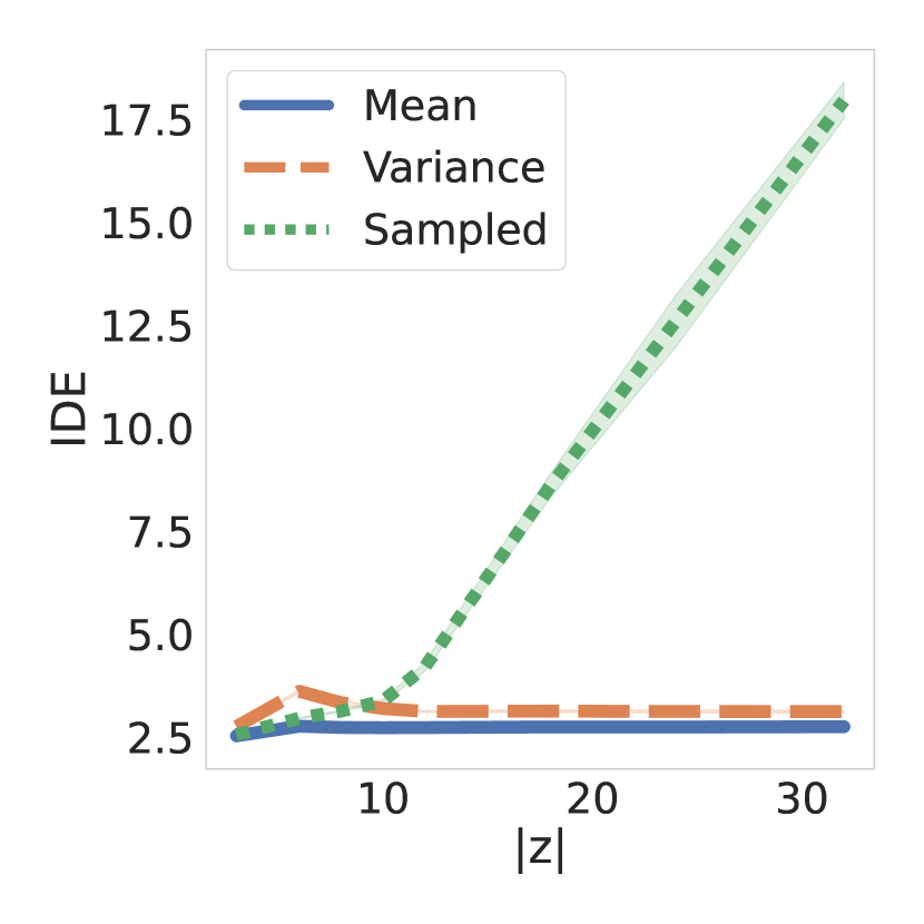
(a) Symsol

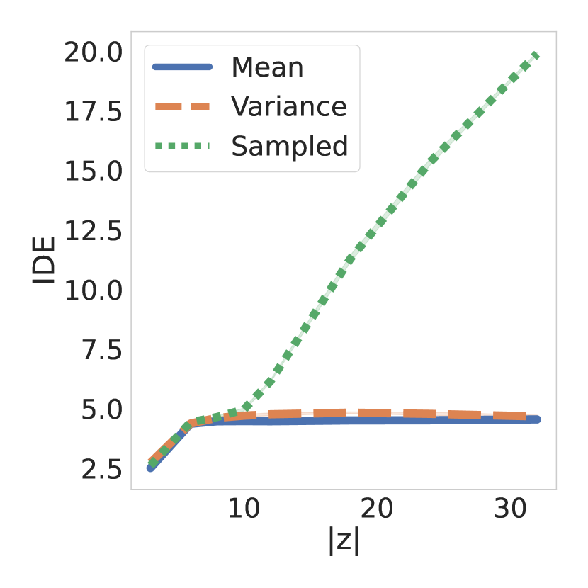
(b) dSprites

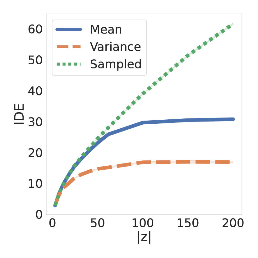
(c) Celeba

Figure 3: Intrinsic dimension estimation of the mean, variance, and sampled representations of VAEs trained with an increasing number of latent dimensions $|{\mathbf{z}}|$. (a), (b), and (c) shows the results on Symsol, dSprites, and Celeba, respectively.

Mean and sampled representations have different IDEs

Looking into the IDEs of mean and sampled representations in Figure 3, we see a clear pattern emerge: when increasing the number of latent variables the IDEs remain similar up to a point, then abruptly diverge. As discussed in Section 2.1, once a VAE has enough latent variables to encode the information needed by the decoder, the remaining variables will become passive to minimise the KL divergence in Equation 2. This phenomenon will naturally occur when we increase the number of latent variables.  Bonheme & Grzes (2021) observed that, in the context of the polarised regime, passive variables were very different in mean and sampled representations. Indeed, for sampled representations, the set of passive variables will be sampled from $\mathcal{N}(0,I)$ where they will stay close to 0 with very low variance in mean representations. They also introduced the concept of mixed variables — variables that are passive only for some data examples — and shown that they were also leading to different mean and sampled representations, albeit to a minor extent. We can thus hypothesise that the difference between the mean and sampled IDEs grows with the number of mixed and passive variables. This is verified by computing the number of active, mixed, and passive variables using the method of Bonheme & Grzes (2021), as shown in Figure 4.

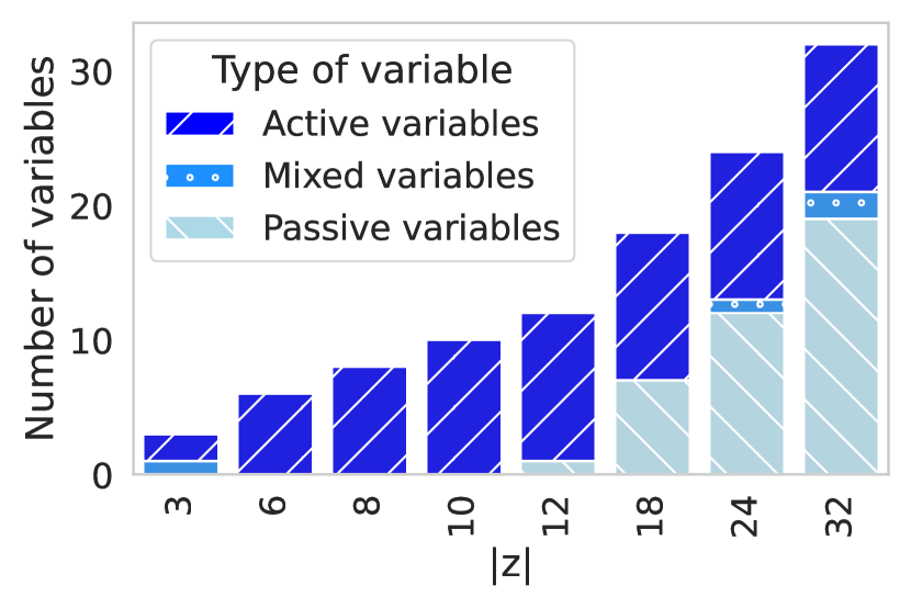
(a) Symsol

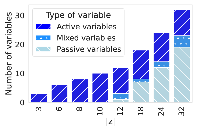
(b) dSprites

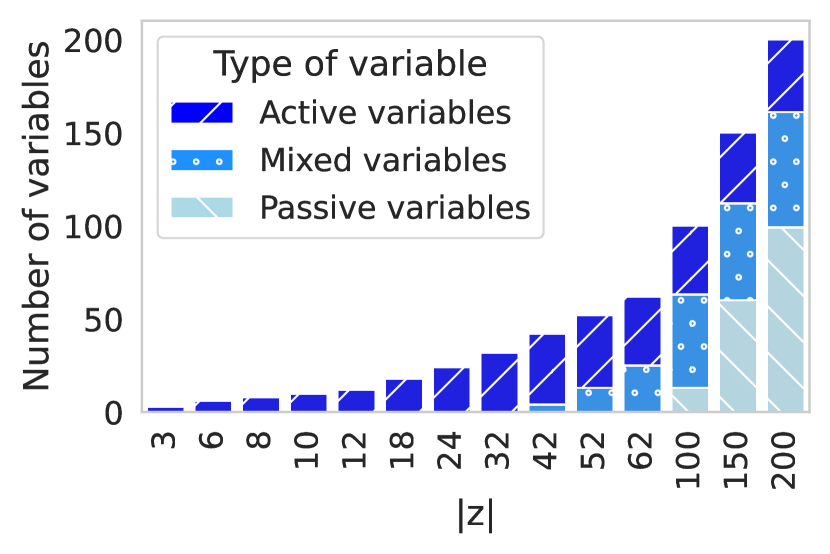
(c) Celeba

Figure 4: Quantity of active, mixed, and passive variables of VAEs trained with an increasing number of latent dimensions $|{\mathbf{z}}|$. (a), (b), and (c) show the results on Symsol, dSprites, and Celeba, respectively.

What happens in the case of posterior collapse?

By using a $\beta$-VAE with very large $\beta$ (e.g., $\beta=20$), one can induce posterior collapse, where a majority of the latent variables become passive and prevent the decoder from accessing sufficient information about the input to provide a good reconstruction. This phenomenon is illustrated in Figure 2(d), where the IDs of the encoder are similar to what one would obtain for a well performing model in the first 5 layers, indicating that these early layers of the encoder still encode some useful information about the data. The IDs then drop in the last three layers of the encoder, indicating that most variables are passive, and only a very small amount of information is retained. The ID of the sampled representation (see sampled in  Figure 2(d)) is then artificially inflated by the passive variables and becomes very close to the number of dimensions $|{\mathbf{z}}|$. From this, the decoder is unable to learn much and has thus a low ID, close to the ID of the mean representation (see the points on the RHS of Figure 2(d)).

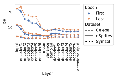
Figure 5: The evolution over multiple epochs of the IDE of the representations learned by VAEs using 10 latent variables on Symsol, dSprites, and Celeba.

The IDs of the model’s representations do not change much after the first epoch

The IDs of the different layers do not change much after the first epoch for well-performing models (see Figure 5). However, for Celeba, whose number of latent dimensions is lower than the data IDE and thus cannot reconstruct the data well, the ID tends to change more in the early layers of the encoder, with a higher variance in IDE.

4.3 Finding the optimal number of dimensions by unsupervised estimation

As discussed in Section 4.2, the IDs of the mean and sampled representations start to diverge when (unused) passive variables appear, and this is already visible after the first epochs of training. We can thus use the difference of IDs between the mean and sampled representations to find the number of latent dimensions retaining the most information while remaining sufficiently compressed (i.e., no passive variables). To this aim, we propose an algorithm for Finding the Optimal Number of Dimensions from Unsupervised Estimation (FONDUE).

Theorem 1.

Any execution of FONDUE (Algorithm 1) returns the largest number of dimensions $p$ for which $IDE_{z}-IDE_{\mu}\leqslant threshold$, where $IDE_{z}$, and $IDE_{\mu}$ are the IDEs of the sampled and mean representations, respectively.

Proof Sketch.

In Algorithm 1, we define a lower and upper bound of the ID estimate, $l$ and $u$, and update the predicted number of latent variables $p$ until, after $i$ iterations, $p_{i}=l_{i}$. Using the loop invariant $l_{i}\leqslant p_{i}\leqslant u_{i}$, we can show that the algorithm terminates when $l_{i}=p_{i}=\operatorname{floor}\left(\frac{l_{i}+u_{i}}{2}\right)$, which can only be reached when $u_{i}=p_{i}+1$, that is, when $p_{i}$ is the maximum number of latent dimensions for which we have $IDE_{z}-IDE_{\mu}\leqslant threshold$. See Appendix A for the full proof. ∎

To ensure stable ID estimates, we computed FONDUE multiple times, gradually increasing the number of epochs $e$ until the predicted $p$ stopped changing. As reported in Table 1, the results were already stable after one epoch, except for Symsol which needed two. We set a fixed threshold $t=0.2$ (20% of the data IDE) in all our experiments and used memoisation (see Algorithm 2) to avoid unnecessary retraining and speed up Algorithm 1.

Algorithm 1 FONDUE

1:procedure FONDUE($t,IDE_{data},epochs$)

2:     $l\leftarrow 0$ $\triangleright$ Lower bound

3:     $u\leftarrow\infty$ $\triangleright$ Upper bound

4:     $p\leftarrow IDE_{data}$ $\triangleright$ Current number of latent dimensions

5:     $mem\leftarrow\{\}$

6:     $threshold\leftarrow\frac{t\times p}{100}$

7:     while $p\neq l$ do

8:         $IDE_{z},IDE_{\mu}\leftarrow\operatorname{GET-MEM}(mem,p,epochs)$

9:         if $IDE_{z}-IDE_{\mu}\leqslant threshold$ then $\triangleright$ Figure 6

10:              $l\leftarrow p$

11:              $p\leftarrow\min(p\times 2,u)$

12:         else$\triangleright$ Figure 7

13:              $u\leftarrow p$

14:              $p\leftarrow\operatorname{floor}\left(\frac{l+u}{2}\right)$

15:         end if

16:     end while

17:     return $p$

18:end procedure

Algorithm 2 GET-MEM

1:procedure GET-MEM($mem,p,e$)

2:     if $mem[p]=\emptyset$ then

3:         $vae\leftarrow\operatorname{TRAIN-VAE}(dim=p,n\_epochs=e)$

4:         $IDE_{z},IDE_{\mu}\leftarrow IDEs(vae)$

5:         $mem[p]\leftarrow IDE_{z},IDE_{\mu}$

6:     end if

7:     return $mem[p]$

8:end procedure

Figure 6: Update $l$ and increase $p$ until $IDE_{z}-IDE_{\mu}>threshold$.

Figure 7: Update $u$ and decrease $p$ until $IDE_{z}-IDE_{\mu}\leqslant threshold$.

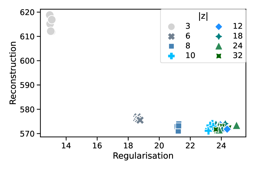
(a) Symsol

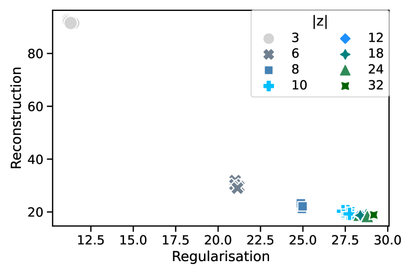
(b) dSprites

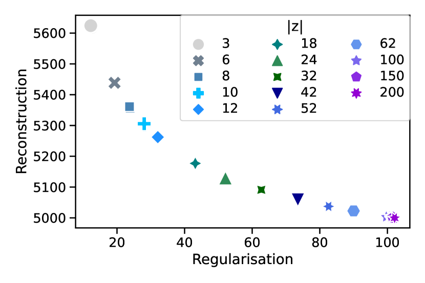
(c) Celeba

Figure 8: Reconstruction and regularisation loss of VAEs for Symsol, dSprites, and Celeba with an increasing number of latent variables.

Table 1: Number of latent variables $|{\mathbf{z}}|$ obtained with FONDUE. The results are averaged over 5 seeds, and computation times are reported for NVIDIA A100 GPUs. The computation time is given for one run of FONDUE over the minimum number of epochs needed to obtain a stable score.

Dataset	Dimensionality (avg $\pm$ SD)	Time/run	Models trained	Epochs/training
Symsol	11 $\pm$ 0	7 min	6	2
dSprites	12.2 $\pm$ 0.4	20 min	5	1
Celeba	50.2 $\pm$ 0.9	14 min	9	1

Analysing the results of FONDUE

As shown in Table 1, the execution time for finding the optimal number of dimensions of a dataset is much shorter than for fully training one model (approximately 2h using the same GPUs), making the algorithm clearly more efficient than grid search. Moreover, the number of latent dimensions predicted by FONDUE is consistent with well-performing models. Indeed, for dSprites and Symsol, the selected numbers of dimensions correspond to the number of dimensions after which the reconstruction error stops decreasing and the regularisation loss remains stable (see Figure 8). For Celeba, the reconstruction loss continues to improve slightly after 50 latent dimensions, due to the addition of mixed variables between 52 and 100 latent dimensions. While one could increase the threshold of FONDUE to take more mixed variables into account, this may not always be desirable. Indeed, mixed variables encode features specific to a subtype of data examples (Bonheme & Grzes, 2021) and will provide less compact representations for a gain in reconstruction quality which may only be marginal.

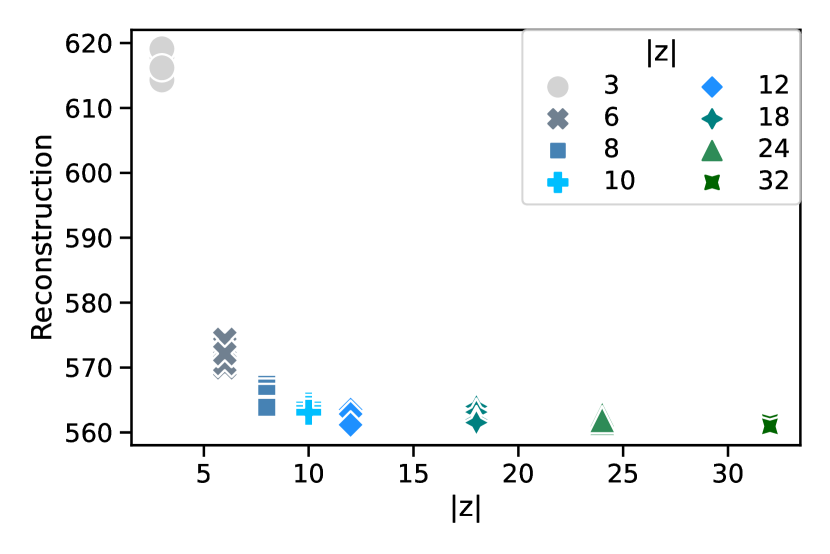
(a) Symsol

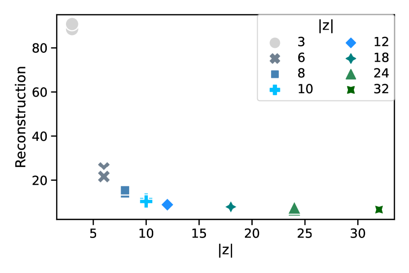
(b) dSprites

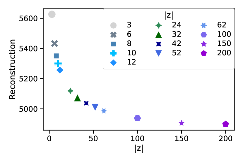
(c) Celeba

Figure 9: Reconstruction loss of AEs for Symsol, dSprites, and Celeba with an increasing number of latent variables.

Can FONDUE be applied to other architectures and learning objectives?

We can see in Figure 9 that deterministic AEs with equivalent architectures to the VAEs in Figure 8 are performing well when provided with the same number of latent dimensions, indicating that FONDUE’s results could be reused for AEs trained on the same dataset with an identical architecture. FONDUE also seems to be robust to architectural changes and worked equally well with fully-connected architectures (see Appendix D).

5 Conclusion

By studying the ID estimates of the representations learned by VAEs, we have seen that the deeper the encoder’s layers, the lower their ID, while the ID of the decoder’s layers consistently stayed close to the ID of the mean representation. We also observed increasing discrepancies between mean and sampled IDs when the number of latent variable was large enough for passive and mixed variables to appear.

This phenomenon is seen very early in the training process, and it leads to FONDUE: an algorithm which can find the number of latent dimensions after which the mean and sampled representations start to strongly diverge. After proving the correctness of our algorithm, we have shown that it is a computationally efficient alternative to grid search — taking only minutes to provide an estimation of the optimal number of dimensions to use — which leads to a good tradeoff between the reconstruction and regularisation losses. Moreover, FONDUE is not impacted by architectural changes, and its prediction can also be used for deterministic autoencoders.

Acknowledgments

The authors thank Théophile Champion and Declan Collins for their helpful comments on the paper.

Appendix A Proof of Theorem 1

This section provides the full proof of Theorem 1. To ease its reading, let us first define an axiom based on our observation from Section 4.2 that the IDEs of the mean and sampled representations start to diverge only after the number of latent dimensions has become large enough for (unused) passive variables to appear.

Axiom 1.

Let $IDE_{x}^{y}$ be the IDE of layer $x$ using $y$ latent dimensions. Given the sets ${\mathbb{A}}=\{a|IDE^{a}_{z}-IDE^{a}_{\mu}\leqslant threshold\}$ and ${\mathbb{B}}=\{b|IDE^{b}_{z}-IDE^{b}_{\mu}>threshold\}$, we have $a<b\quad\forall\,a\in{\mathbb{A}},\;\forall\,b\in{\mathbb{B}}$.

Remark 1.

Given that $l$ and $u$ only take values of latent dimensions for which $IDE_{z}-IDE_{\mu}\leqslant threshold$ and $IDE_{z}-IDE_{\mu}>threshold$, respectively, Axiom 1 implies that for all iterations $i$, $l_{i}\in{\mathbb{A}}$ and $u_{i}\in{\mathbb{B}}$ and $l_{i}<u_{i}$.

Using the loop invariant $l_{i}\leqslant p_{i}\leqslant u_{i}$ for each iteration $i$, we will now show that Algorithm 1 terminates when $l_{i}=p_{i}=\operatorname{floor}\left(\frac{l_{i}+u_{i}}{2}\right)$, which can only be reached when $u_{i}=p_{i}+1$, that is when $p_{i}$ is the maximum number of latent dimensions for which we have $IDE_{z}-IDE_{\mu}\leqslant threshold$.

Proof.

Initialisation: $l_{0}=0,p_{0}=IDE_{data},u_{0}=\infty$, thus $l_{0}<p_{0}<u_{0}$.

Maintenance: We will consider both branches of the if statement separately:

• For $IDE_{z}-IDE_{\mu}\leqslant threshold$ (lines 9-11), $u_{i}=u_{i-1}$, $p_{i}=min(p_{i-1}\times 2,u_{i})$, and $l_{i}=p_{i-1}$. We directly see that $p_{i}\leqslant u_{i}$. We know from Remark 1 that $l_{i}<u_{i}$ and we also have $l_{i}<p_{i-1}\times 2$, it follows that $l_{i}<p_{i}$. Grouping both inequalities, we get $l_{i}<p_{i}\leqslant u_{i}$.

• For $IDE_{z}-IDE_{\mu}>threshold$ (lines 12-14), $u_{i}=p_{i-1},l_{i}=l_{i-1}$, and $p_{i}=\operatorname{floor}\left(\frac{l_{i}+u_{i}}{2}\right)$. Using Remark 1 we can directly see that $l_{i}\leqslant\operatorname{floor}\left(\frac{l_{i}+u_{i}}{2}\right)<u_{i}$ and we obtain $l_{i}\leqslant p_{i}<u_{i}$.

Termination: The loop terminates when $l_{i}=p_{i}$. Given that $l_{i}<p_{i}$ when $IDE_{z}-IDE_{\mu}\leqslant threshold$, this is only possible when $IDE_{z}-IDE_{\mu}>threshold$, which is when $p_{i}=\operatorname{floor}\left(\frac{l_{i}+u_{i}}{2}\right)$. We know from Remark 1 that $l_{i}<u_{i}$, so we must have $(l_{i}+u_{i})\operatorname{mod}2>0$. As $a\operatorname{mod}2\in\{0,1\}$, the only possible value for $u_{i}$ to satisfy $l_{i}=p_{i}=\operatorname{floor}\left(\frac{l_{i}+u_{i}}{2}\right)$ is $u_{i}=p_{i}+1$. Thus, $p_{i}$ is the largest number of latent dimensions for which $IDE_{z}-IDE_{\mu}\leqslant threshold$.

∎

Appendix B Resources

As mentioned in Sections 1 and 3, we released the code of our experiment, and the IDEs:

• The IDEs can be downloaded at https://data.kent.ac.uk/id/eprint/455

• symsol_reduced, the reduced version of Symmetric solids can be downloaded at https://data.kent.ac.uk/436

• The code is available at https://github.com/bonheml/VAE_learning_dynamics

Appendix C Experimental setup

Our implementation uses the same hyperparameters as Locatello et al. (2019), as listed in Table 2. We reimplemented the Locatello et al. (2019) code base, designed for Tensorflow 1, in Tensorflow 2 using Keras. The model architectures used are also similar, as described in Table 3 and 4. We used the convolutional architecture in the main paper and the fully-connected architecture in Appendix D. Each model is trained 5 times with seed values from 0 to 4. Every image input is normalised to have pixel values between 0 and 1. TwoNN is used with an anchor of 0.9, and the hyperparameters for MLE can be found in Table 5.

Table 2: VAEs hyperparameters

Parameter	Value
Batch size	64
Latent space dimension	3, 6, 8, 10, 12, 18, 24, 32.
	For Celeba only: 42, 52, 62, 100, 150, 200
Optimizer	Adam
Adam: $\beta_{1}$	0.9
Adam: $\beta_{2}$	0.999
Adam: $\epsilon$	1e-8
Adam: learning rate	0.0001
Reconstruction loss	Bernoulli
Training steps	300,000
Train/test split	90/10
$\beta$	1

Table 3: Architecture

Encoder	Decoder
Input: $\mathbb{R}^{64\times 63\times channels}$	$\mathbb{R}^{10}$
Conv, kernel=4×4, filters=32, activation=ReLU, strides=2	FC, output shape=256, activation=ReLU
Conv, kernel=4×4, filters=32, activation=ReLU, strides=2	FC, output shape=4x4x64, activation=ReLU
Conv, kernel=4×4, filters=64, activation=ReLU, strides=2	Deconv, kernel=4×4, filters=64, activation=ReLU, strides=2
Conv, kernel=4×4, filters=64, activation=ReLU, strides=2	Deconv, kernel=4×4, filters=32, activation=ReLU, strides=2
FC, output shape=256, activation=ReLU, strides=2	Deconv, kernel=4×4, filters=32, activation=ReLU, strides=2
FC, output shape=2x10	Deconv, kernel=4×4, filters=channels, activation=ReLU, strides=2

Table 4: Fully-connected architecture

Encoder	Decoder
Input: $\mathbb{R}^{64\times 63\times channels}$	$\mathbb{R}^{10}$
FC, output shape=1200, activation=ReLU	FC, output shape=256, activation=tanh
FC, output shape=1200, activation=ReLU	FC, output shape=1200, activation=tanh
FC, output shape=2x10	FC, output shape=1200, activation=tanh

Table 5: MLE hyperparameters

Parameter	Value
k	3, 5, 10, 20
anchor	0.8
seed	0
runs	5

Appendix D FONDUE on fully-connected architectures

We report the results obtained by FONDUE for fully-connected (FC) architectures in Table 6 and Figure 10. As shown in Table 6, the execution time for finding the optimal number of dimensions of a dataset is much shorter than for training one model (this is approximately 2h on the same GPUs), in similarity with convolutional VAEs. As in Section 4.3, FONDUE correctly finds the number of latent dimensions after which the mean and sampled IDEs start to diverge, as shown in Figure 10. One can see that the number of latent variables needed for FC VAEs is much lower than for convolutional VAEs (see Table 1 for comparison). For dSprites, it is near the true ID of the data, and for Celeba, it is close to the data IDE reported in Figure 1 of Section 4.1.

As in Section 4.3, we gradually increase the number of epochs until FONDUE reaches a stable estimation of the latent dimensions. As these models have fewer parameters than the convolutional architecture used in Section 4.3, they converge more slowly and need to be trained for more epochs on Celeba and Symsol before reaching a stable estimation (Arora et al., 2018; Sankararaman et al., 2020). dSprites contains more data examples than the other datasets and less complex data than Celeba, which can explain its quicker convergence.

For dSprites and Symsol, the number of dimensions selected by FONDUE corresponds to the number of dimensions after which the reconstruction stops improving and the regularisation loss remains stable (see Figure 11). For Celeba, the reconstruction continues to improve slightly after 39 latent dimensions, due to the addition of variables between 42 and 100 latent dimensions, as illustrated in Figure 12. As in convolutional architectures, one could increase the threshold of FONDUE to take more mixed variables into account.

Overall, we can see that FONDUE also provides good results on the FC architectures, despite a slower convergence, showing robustness to architectural changes.

Table 6: Number of latent variables obtained with FONDUE for fully-connected architectures. The results are averaged over 5 seeds, and computation times are reported for NVIDIA A100 GPUs. The computation time is given for one run of FONDUE over the minimum number of epochs needed to obtain a stable score.

Dataset	Dimensionality (avg $\pm$ SD)	Time/run	Models trained	Epochs/training
Symsol	8 $\pm$ 0	15 min	6	6
dSprites	6.6 $\pm$ 0.5	16 min	5	1
Celeba	39 $\pm$ 0.6	50 min	7	9

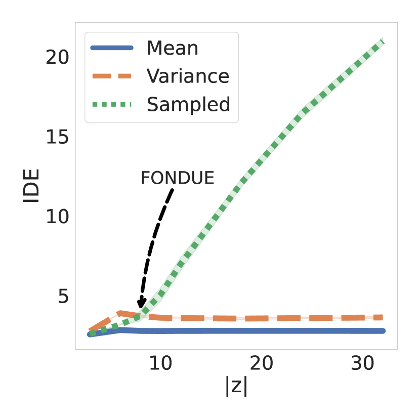
(a) Symsol

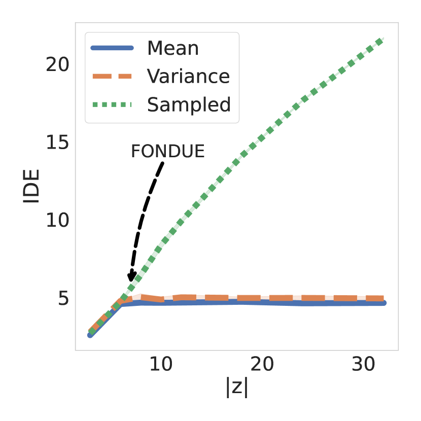
(b) dSprites

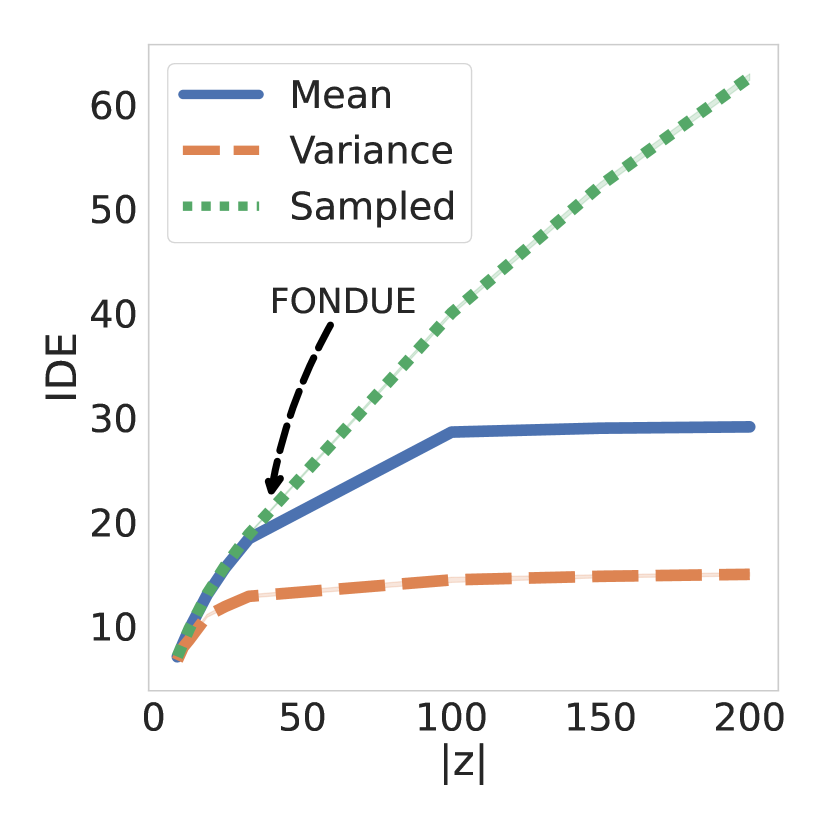
(c) Celeba

Figure 10: Number of latent dimensions provided by FONDUE for fully-connected VAEs: $|{\mathbf{z}}|=8$ on Symsol, $|{\mathbf{z}}|=7$ on dSprites, and $|{\mathbf{z}}|=39$ on Celeba.

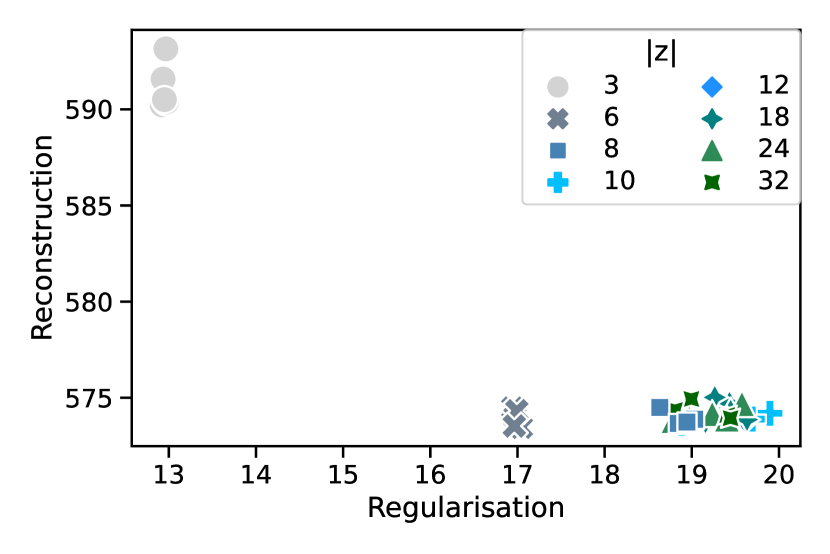
(a) Symsol

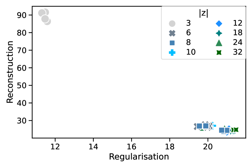
(b) dSprites

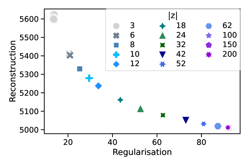
(c) Celeba

Figure 11: Reconstruction and regularisation scores of fully-connected VAEs for Symsol, dSprites, and Celeba with an increasing number of latent variables $|{\mathbf{z}}|$.

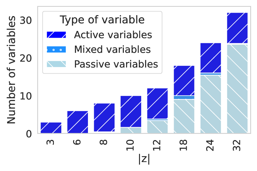
(a) Symsol

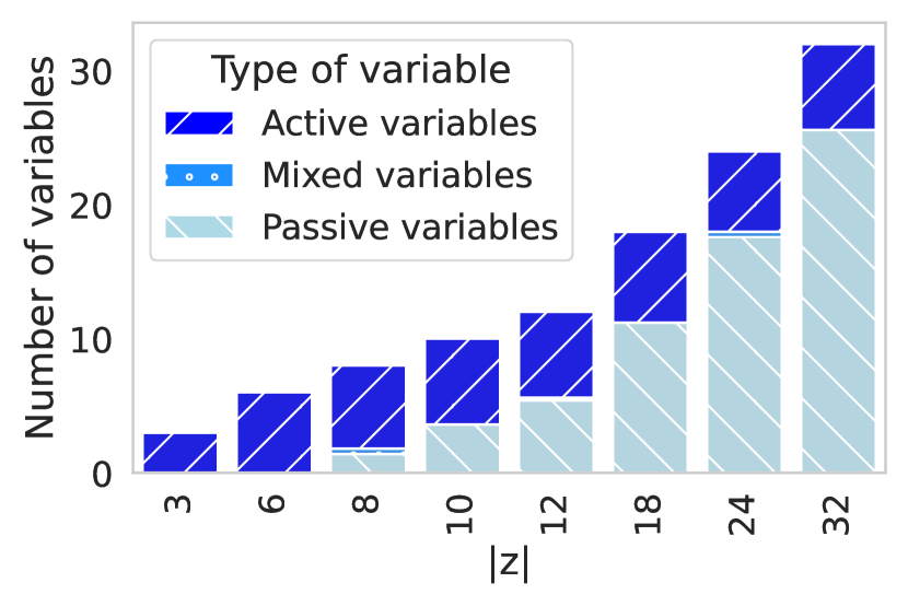
(b) dSprites

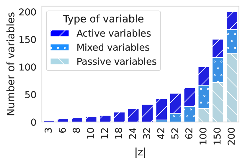
(c) Celeba

Figure 12: Quantity of active, mixed, and passive variables of VAEs trained with an increasing number of latent dimensions $|{\mathbf{z}}|$. (a), (b), and (c) show the results on Symsol, dSprites, and Celeba, respectively.

Appendix E Additional details on mean, variance, and sampled representations

This section presents a concise illustration of what mean, variance, and sampled representations are. As shown in Figure 13, the mean, variance and sampled representations are the last 3 layers of the encoder, where the sampled representation, ${\mathbf{z}}$, is the input of the decoder.

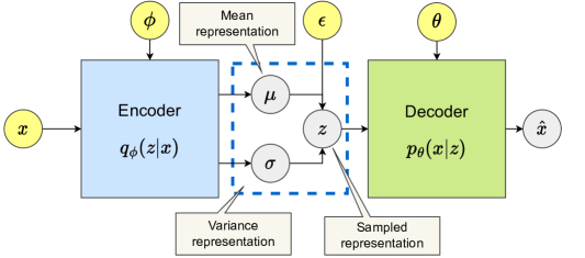
Figure 13: The structure of a VAE

Appendix F Passive variables and posterior collapse

As discussed in Section 2.1, passive variables appear in latent representations of VAEs in two cases: polarised regime and posterior collapse. In well-behaved VAEs (i.e., in the case of polarised regime), passive variables arise when the number of latent dimensions is larger than the number of latent variables needed by the VAE to encode latent representations. These passive variables contribute to lowering the regularisation loss term of Equation 1 without increasing the reconstruction loss. However, passive variables can also be encountered as part of a pathological state where the reconstruction loss is very high and the regularisation loss is pushed towards zero (i.e., when posterior collapse takes place). This issue can happen for various reasons (Dai et al., 2020), but is clearly distinct from the polarised regime as the reconstruction loss is very high and the latent representations contain little to no active variables.

In both cases, passive variables are very different in mean and sampled representations, due to the sampling process ${\mathbf{z}}\sim{\bm{\mu}}+\epsilon\sqrt{{\sigma}{\bm{I}}}$, where $\epsilon\sim\mathcal{N}(0,{\bm{I}})$, ${\bm{\mu}}$ is the mean representation and ${\sigma}{\bm{I}}$ the diagonal matrix of the variance representations. For the regularisation term to be low, one needs to create passive variables, that is, as many dimensions of ${\mathbf{z}}$ as close as possible to $\mathcal{N}(0,{\bm{I}})$. This can easily be done by setting some elements of ${\bm{\mu}}$ to 0 and their corresponding variance to 1. As a result, passive variables, when observed over multiple data examples will have a mean of 0 in the mean and sampled representations. However, their variance will be close to 0 in the mean representations, and close to 1 in their sampled counterpart (Rolinek et al., 2019; Bonheme & Grzes, 2021).

Appendix G Why not use variable type instead of IDE for FONDUE?

As passive variables are easy to detect, one could wonder why they were not used directly to determine the number of latent dimensions instead of comparing IDEs of models trained for a few epochs multiple times. For example, it would be quicker to train one model with a large number of latent variables for a few epochs and retrieve the number of active (or active and mixed) variables detected, as for example, illustrated in Algorithm 3.

How does Algorithm 3 work?

We define the initial number of latent variables as twice the data IDE. Then, if we want to have enough dimensions for active and mixed variables, we double the number of latent variables until we find at least one passive variable and return the sum of active and mixed variables as the chosen number of latent dimensions. If we want instead to have only active variables, we double the number of latent variables until we find at least either one passive or mixed variable and return the number of active variables as the chosen number of latent dimensions.

Why use Algorithm 1 instead?

As shown in Table 7, the identification of variable types displays a high variance during early training, which generally makes Algorithm 3 less reliable than Algorithm 1 for equivalent computation time. In addition to this instability, the numbers of latent dimensions predicted by Algorithm 3 in Table 7 are far from optimal compared to Table 1. There is a large overestimation in Symsol and an underestimation in Celeba. These issues may be explained by the fact that Algorithm 1 is based on mean and sampled representations, while Algorithm 3 solely relies on variance representations, decreasing the stability during early training. Moreover, mixed and passive variables are not discriminated correctly in early epochs, possibly for the same reasons, preventing any modulation of compression/reconstruction quality that could be achieved with Algorithm 1.

Algorithm 3 FONDUE with variable types

procedure FONDUE-var($data\_ide,epochs,keep\_mixed$)

     $l\leftarrow 2*data\_ide$

     $n\leftarrow-1$

     while $n<0$ do

         $vae\leftarrow train\_VAE(dim=l,n\_epochs=epochs)$

         $av,mv,pv\leftarrow variable\_types(vae)$ $\triangleright$ Number of active, mixed and passive variables

         if $pv>0$ and $keep\_mixed$ then

              $n\leftarrow av+mv$

         else if ($mv>0$ or $pv>0$) and not $keep\_mixed$ then

              $n\leftarrow av$

         else

              $l\leftarrow l*2$

         end if

     end while

     return $n$

end procedure

Table 7: Number of latent variables obtained with FONDUE-var. The results are averaged over 5 seeds and computation times are reported for NVIDIA A100 GPUs.

Dataset	Dimensionality (avg $\pm$ SD)	Time/run	Models trained	Epochs/training
Symsol	14 $\pm$ 1.2	2 min	3	1
Symsol	17 $\pm$ 1.7	3 min	3	2
Symsol	15 $\pm$ 1.1	10 min	3	5
dSprites	9.2 $\pm$ 1.3	4 min	1	1
dSprites	8.8 $\pm$ 1.2	8 min	1	2
dSprites	9.6 $\pm$ 0.5	20 min	1	5
Celeba	38.6 $\pm$ 2.6	1 min	1	1
Celeba	38.6 $\pm$ 0.4	2 min	1	2
Celeba	41.2 $\pm$ 0.4	6 min	1	5

References

- Ansuini et al. (2019) Alessio Ansuini, Alessandro Laio, Jakob H. Macke, and Davide Zoccolan. Intrinsic dimension of data representations in deep neural networks. In Advances in Neural Information Processing Systems, volume 32, 2019.
- Arora et al. (2018) Sanjeev Arora, Nadav Cohen, and Elad Hazan. On the optimization of deep networks: Implicit acceleration by overparameterization. In Jennifer Dy and Andreas Krause (eds.), Proceedings of the 35th International Conference on Machine Learning, volume 80 of Proceedings of Machine Learning Research, pp. 244–253. PMLR, 2018.
- Arvanitidis et al. (2018) Georgios Arvanitidis, Lars Kai Hansen, and Søren Hauberg. Latent Space Oddity: on the Curvature of Deep Generative Models. In International Conference on Learning Representations, volume 6, 2018.
- Bonheme & Grzes (2021) Lisa Bonheme and Marek Grzes. Be More Active! Understanding the Differences between Mean and Sampled Representations of Variational Autoencoders. arXiv e-prints, 2021.
- Campadelli et al. (2015) P. Campadelli, E. Casiraghi, C. Ceruti, and A. Rozza. Intrinsic dimension estimation: Relevant techniques and a benchmark framework. Mathematical Problems in Engineering, 2015, 2015.
- Chollet (2021) F. Chollet. Deep Learning with Python, Second Edition. Manning, 2021. ISBN 9781617296864.
- Dai & Wipf (2018) Bin Dai and David Wipf. Diagnosing and Enhancing VAE Models. In International Conference on Learning Representations, volume 6, 2018.
- Dai et al. (2020) Bin Dai, Ziyu Wang, and David Wipf. The Usual Suspects? Reassessing Blame for VAE Posterior Collapse. In Proceedings of the 37th International Conference on Machine Learning, 2020.
- Doersch (2016) Carl Doersch. Tutorial on Variational Autoencoders. arXiv e-prints, 2016.
- Facco et al. (2017) Elena Facco, Maria dÉrrico, Alex Rodriguez, and Alessandro Laio. Estimating the intrinsic dimension of datasets by a minimal neighborhood information. Scientific Reports, 7(1), 2017.
- Falorsi et al. (2018) Luca Falorsi, Pim De Haan, Tim R Davidson, Nicola De Cao, Maurice Weiler, Patrick Forré, and Taco S Cohen. Explorations in homeomorphic variational auto-encoding. arXiv e-prints, 2018.
- Gong et al. (2019) Sixue Gong, Vishnu Naresh Boddeti, and Anil K Jain. On the intrinsic dimensionality of image representations. In Proceedings of the IEEE/CVF Conference on Computer Vision and Pattern Recognition, pp. 3987–3996, 2019.
- Hensel et al. (2021) Felix Hensel, Michael Moor, and Bastian Rieck. A survey of topological machine learning methods. Frontiers in Artificial Intelligence, 4, 2021.
- Higgins et al. (2017) Irina Higgins, Loic Matthey, Arka Pal, Christopher Burgess, Xavier Glorot, Matthew Botvinick, Mohamed Shakir, and Alexander Lerchner. -VAE: Learning Basic Visual Concepts with a Constrained Variational Framework. In International Conference on Learning Representations, volume 5, 2017.
- Karbauskaitė et al. (2011) Rasa Karbauskaitė, Gintautas Dzemyda, and Edmundas Mazėtis. Geodesic distances in the maximum likelihood estimator of intrinsic dimensionality. Nonlinear Analysis, 16(4):387–402, 2011.
- Keller & Welling (2021) T. Anderson Keller and Max Welling. Topographic VAEs learn equivariant capsules. In A. Beygelzimer, Y. Dauphin, P. Liang, and J. Wortman Vaughan (eds.), Advances in Neural Information Processing Systems, volume 35, 2021.
- Khrulkov & Oseledets (2018) Valentin Khrulkov and Ivan Oseledets. Geometry score: A method for comparing generative adversarial networks. In Jennifer Dy and Andreas Krause (eds.), Proceedings of the 35th International Conference on Machine Learning, volume 80 of Proceedings of Machine Learning Research, pp. 2621–2629. PMLR, 10–15 Jul 2018.
- Kingma & Welling (2014) Diederik P. Kingma and Max Welling. Auto-Encoding Variational Bayes. In International Conference on Learning Representations, volume 2, 2014.
- Levina & Bickel (2004) Elizaveta Levina and Peter J. Bickel. Maximum Likelihood Estimation of Intrinsic Dimension. In Advances in Neural Information Processing Systems, volume 16, 2004.
- Liu et al. (2015) Ziwei Liu, Ping Luo, Xiaogang Wang, and Xiaoou Tang. Deep learning face attributes in the wild. In ICCV, 2015.
- Locatello et al. (2019) Francesco Locatello, Stefan Bauer, Mario Lucic, Gunnar Raetsch, Sylvain Gelly, Bernhard Schölkopf, and Olivier Bachem. Challenging Common Assumptions in the Unsupervised Learning of Disentangled Representations. In Proceedings of the 36th International Conference on Machine Learning, volume 97 of Proceedings of Machine Learning Research, 2019.
- Lucas et al. (2019a) James Lucas, George Tucker, Roger B. Grosse, and Mohammad Norouzi. Understanding Posterior Collapse in Generative Latent Variable Models. In Deep Generative Models for Highly Structured Data, ICLR 2019 Workshop, 2019a.
- Lucas et al. (2019b) James Lucas, George Tucker, Roger B. Grosse, and Mohammad Norouzi. Don’t Blame the ELBO! A linear VAE Perspective on Posterior Collapse. In Advances in Neural Information Processing Systems, volume 32, 2019b.
- MacKay & Ghahramani (2005) David J.C. MacKay and Zoubin Ghahramani. Comments on ‘Maximum Likelihood Estimation of Intrinsic Dimension’ by E. Levina and P. Bickel (2004), 2005. URL http://www.inference.org.uk/mackay/dimension/.
- Maheswaranathan et al. (2019) Niru Maheswaranathan, Alex Williams, Matthew Golub, Surya Ganguli, and David Sussillo. Universality and Individuality in Neural Dynamics Across Large Populations of Recurrent Networks. In Advances in Neural Information Processing Systems, volume 32, 2019.
- Murphy et al. (2021) Kieran Murphy, Carlos Esteves, Varun Jampani, Srikumar Ramalingam, and Ameesh Makadia. Implicit representation of probability distributions on the rotation manifold. In International Conference on Machine Learning, 2021.
- Naitzat et al. (2020) Gregory Naitzat, Andrey Zhitnikov, and Lek-Heng Lim. Topology of Deep Neural Networks. Journal of Machine Learning Research, 21(184), 2020.
- Perez Rey et al. (2020) Luis A. Perez Rey, V. Menkovski, and Jacobus W. Portegies. Diffusion Variational Autoencoders. In 29th International Joint Conference on Artificial Intelligence - 17th Pacific Rim International Conference on Artificial Intelligence. (IJCAI-PRICAI 2020), 2020.
- Pope et al. (2021) Phillip Pope, Chen Zhu, Ahmed Abdelkader, Micah Goldblum, and Tom Goldstein. The Intrinsic Dimension of Images and Its Impact on Learning. In International Conference on Learning Representations, volume 9, 2021.
- Rezende & Mohamed (2015) Danilo Rezende and Shakir Mohamed. Variational Inference with Normalizing Flows. In Proceedings of the 32nd International Conference on Machine Learning, volume 37 of Proceedings of Machine Learning Research, 2015.
- Rieck et al. (2019) Bastian Rieck, Matteo Togninalli, Christian Bock, Michael Moor, Max Horn, Thomas Gumbsch, and Karsten Borgwardt. Neural Persistence: A Complexity Measure for Deep Neural Networks Using Algebraic Topology. In International Conference on Learning Representations, volume 7, 2019.
- Rolinek et al. (2019) Michal Rolinek, Dominik Zietlow, and Georg Martius. Variational Autoencoders Pursue PCA Directions (by Accident). In Proceedings of the IEEE/CVF Conference on Computer Vision and Pattern Recognition (CVPR), 2019.
- Sankararaman et al. (2020) Karthik Abinav Sankararaman, Soham De, Zheng Xu, W. Ronny Huang, and Tom Goldstein. The impact of neural network overparameterization on gradient confusion and stochastic gradient descent. In Hal Daumé III and Aarti Singh (eds.), Proceedings of the 37th International Conference on Machine Learning, volume 119 of Proceedings of Machine Learning Research, pp. 8469–8479. PMLR, 2020.
- Zhou et al. (2021) Sharon Zhou, Eric Zelikman, Fred Lu, Andrew Y. Ng, Gunnar E. Carlsson, and Stefano Ermon. Evaluating the disentanglement of deep generative models through manifold topology. In International Conference on Learning Representations, volume 9, 2021.