Multi-wavelength Observations of MWC 297: Constraints on Disk Inclination and Mass Outflow

Abstract

MWC 297 is a young, early-type star driving an ionized outflow and surrounded by warm, entrained dust. Previous analyses of near- and mid-IR interferometric images suggest that the emission at these wavelengths arises from a compact accretion disk with a moderate ($i<$ 40^∘) inclination. We have obtained 5-40 $\mu$m images of MWC 297 with FORCAST on SOFIA, as well as near-infrared spectra acquired with SpeX on the IRTF and radio data obtained with the VLA and BIMA, and supplemented these with archival data from Herschel/PACS and SPIRE. The FORCAST images, combined with the VLA data, indicate that the outflow lobes are aligned nearly north-south and are well separated. Simple geometrical modeling of the FORCAST images suggests that the disk driving the outflow has an inclination of $55\pm 5$^∘, in disagreement with the results of the interferometric analyses. Analysis of the SpeX data, with a wind model, suggests the the mass loss rate is on the order of $6.0\pm^{3.7}_{1.7}\times 10^{-7}M_{\odot}~{}\mathrm{yr}^{-1}$ and the extinction to the source is $A_{V}\sim 8.1\pm^{2.5}_{1.5}$ mag. We have combined our data with values from the literature to generate the spectral energy distribution of the source from $0.35~{}\mu$m to $6$ cm and estimate the total luminosity. We find the total luminosity to be about $7900~{}L_{\odot}$, if we include emission from an extended region around the star, only slightly below that expected for a B1.5V star. The reddening must be produced by dust along the line of sight, but distant from the star.

1 Introduction

As the more massive (2-10 $M_{\odot}$; Waters & Waelkens 1998) counterparts of the low-mass Classical T Tauri Stars, Herbig AeBe (HAeBe) stars represent a bridge between low mass young stellar objects, whose formation processes are (at least qualitatively) well characterized and understood, and high mass stars, whose formation processes are (quite literally) still shrouded in dust and uncertainty. Therefore they represent a means of testing whether the low mass star formation paradigm can be extended to higher mass stars. While it is clear that these young, pre-main sequence stars are actively accreting material from their circumstellar environments, the geometry of the material and the mechanisms by which the accretion occurs are still not well understood, particularly for the most massive Herbig Be systems. Although it is generally agreed that a circumstellar accretion disk is present in these systems (for which there is direct observational evidence in a few cases), the structure and extent of the disks are topics of active research and debate.

MWC 297 is a young ($\sim 0.1$ Myr), highly reddened (A_V $\sim$ 8 mag), rapidly rotating ($v\sin i\sim 350$ km s^-1) early-type (B1.5 Ve) HAeBe star with a luminosity of $L>3\times$ 10³  L_⊙  (Drew et al., 1997; Benedettini et al., 2001; Fairlamb et al., 2015) at a distance of $417.9\pm 5.3$ pc (based on Gaia; Riello et al. 2021). The estimated distance places MWC 297 in the Aquila Rift (Ortiz-León et al., 2017) and beyond the unrelated, foreground H II region Sh 2-62 (Drew et al., 1997). MWC 297 exhibits a strong infrared excess due to hot dust in a circumstellar disk and surrounding envelope (Hillenbrand et al., 1992). It is one of the few early-type B stars known to be surrounded by a circumstellar disk from which it is actively accreting, as evidenced by strong and variable Balmer line emission and double-peaked CO emission (Finkenzeller & Mundt, 1984; Drew et al., 1997; Banzatti et al., 2022; Sandell & Vacca, 2022). It was included in Herbig’s original list of HAeBe stars (Herbig, 1960) as well as in the comprehensive catalogue of HAeBe members and candidate members compiled by Thé, de Winter and Pérez (1994). Analysis of 2MASS and (saturated) Spitzer IRAC images indicates that MWC 297 is the most massive member in a cluster of $\sim$ 80 PMS stars (Wang & Looney, 2007; Gutermuth et al., 2009). Recent high-resolution near-infrared imaging observations have revealed the presence of two possible low-mass ($<0.5M_{\odot}$ companions within 250 AU of MWC 297 (Ubeira-Gabellini et al., 2020; Sallum et al., 2021). MWC 297 has been observed across the electromagnetic spectrum and the literature on it is extensive. A summary of some of the results of previous observations can be found in Acke et al. (2008).

Because MWC 297 is so bright ($K\sim 3$ mag), with strong emission lines, and relatively nearby (for a massive star), it has frequently been the target of near-infrared (NIR) and mid-infrared (MIR) interferometric observations. However, analyses of these, as well as other, observations of MWC 297 have led to contradictory results regarding the inclination $i$ of the accretion disk surrounding it. Based on the extended nature of the source in a 5 GHz radio map, as well as the high value of $v\sin i$ derived from the optical spectra, Drew et al. (1997) initially suggested that the inclination of the system was very high and seen nearly edge-on. The N-S elongation of the source seen in the radio maps of Sandell, Weintraub & Hamidouche (2011) also suggests that the the disk is highly inclined (nearly edge-on with $i>80$ ^∘). However, the double-peaked optical [O I] emission lines detected by Zickgraf (2003) are more indicative of an intermediate inclination for the system. On the other hand, the narrowness of the [O I] lines observed by Acke et al. (2005) led to the conclusion that, if these lines arise from the bipolar outflow, as is typical of Herbig Be stars, then outflow axis should be in the plane of the sky and the system should be viewed nearly edge-on (Acke et al., 2008). Interpretation of the NIR, MIR, and mm interferometric results by numerous authors, however, indicates a fairly low inclination for the system ($i<40$^∘and in some cases as low as $20$^∘; Millan-Gabet at al. 2001; Malbet et al. 2007; Acke et al. 2008; Alonso-Albi et al. 2009; Weigelt et al. 2011; Hone et al. 2017; Kluska et al. 2020). Recently, Sallum et al. (2021) used the Large Binocular Telescope Interferometer to image MWC 297 and derived an inclination angle $\sim$ 50^∘ - 65^∘ under the assumption that the source consisted of a disk plus an outflow at moderate inclination angles. Finally, Oudmaijer & Drew (1999) found no evidence for variation in the spectro-polarimetric signal across the H$\alpha$ line, a result which seems to indicate that the projection of the H $\alpha$ emission region in MWC 297 onto the plane of the sky is circularly symmetric (that is, the system is seen nearly pole-on, with $i\approx 0$^∘). The discrepancy in the derived inclination angles is not merely a trivial detail, as the value can have profound consequences for our understanding of this object. Given the $v\sin i$ value of 350 km s^-1found by Drew et al. (1997), an inclination $i<40$^∘, would imply a stellar rotational velocity close to or even in excess of the critical, or break-up, velocity for such a massive star ($\sim 10$ M_⊙).

In this paper we present mid-infrared images of MWC 297 obtained with the Faint Object infraRed Camera for the SOFIA Telescope (FORCAST) on the Stratospheric Observatory for Infrared Astronomy (SOFIA) as well as previously unpublished NRAO/Very Large Array (VLA) and Berkeley-Illinois-Maryland Association (BIMA) millimeter array observatory data. These observations show that the star drives an ionized jet surrounded by warm entrained dust. The morphology of the outflow, as seen in these images, clearly rules out a face-on disk. We combine these data with Herschel archival data to construct the spectral energy distribution of the system and determine the total luminosity. We also present a medium resolution (R $\sim$ 2000) 0.8 - 2.4 $\mu$m spectrum of MWC 297 obtained with SpeX at the IRTF and use these data to better constrain the properties of the outflow (velocity and mass-loss rate) from the star.

We describe the observations in increasing order of wavelength in the next section. We then present results of attempts to reproduce the morphology seen in the VLA and FORCAST images with a simple physical model. We find that the inclination of the system must be much larger than that derived from the interferometric measurements. We also present the results of a wind model constructed to determine the physical parameters of the outflow. A discussion of these results and our conclusions are given in the final section.

2 Observations and Data Reduction

2.1 IRTF/SpeX observations

We observed MWC 297 at the NASA Infrared Telescope Facility (IRTF) on Mauna Kea on 2007 Nov 02 (UT) with SpeX, the facility near-infrared medium resolution cross-dispersed spectrograph (Rayner et al., 2003). Ten individual exposure of MWC 297, each lasting 30 s, were obtained using the short-wavelength cross-dispersed (SXD) mode of SpeX. This mode yields spectra spanning the wavelength range 0.8 -2.4 $\mu$m divided into 6 spectral orders. The observations were acquired in “pair mode”, in which the object was observed at two separate positions along the 15^′′-long slit. The slit width was set to 0$\farcs$3, which yields a nominal resolving power of 2000 for the SXD spectra. (At the distance of MWC  297 of 418 pc, the SpeX $0\farcs 3$ slit spans $\sim 125$ au.) The slit was set to the parallactic angle during the observations. The airmass was about 1.43 for the observations. Observations of HD 171149, an A0 V star, used as a “telluric standard” to correct for absorption due to the Earth’s atmosphere and to flux calibrate the target spectra, were obtained immediately after the observations of MWC 297. The airmass difference between the observations of the object and the standard was 0.05. Conditions were reported to be rather poor during the observations, with fog present. A set of internal flat fields and arc frames were obtained immediately after the observations of MWC  297 for flat fielding and wavelength calibration purposes.

The data were reduced using Spextool (Cushing, Vacca & Rayner, 2004), the IDL-based package developed for the reduction of SpeX data. The Spextool package performs non-linearity corrections, flat fielding, image pair subtraction, aperture definition, optimal extraction, and wavelength calibration. The sets of spectra resulting from the individual exposures were median combined and then corrected for telluric absorption and flux calibrated using the extracted A0  V telluric standard spectra and the technique and software described by Vacca, Cushing & Rayner (2003). The spectra from the individual orders were then spliced together by matching the flux levels in the overlapping wavelength regions, and regions of poor atmospheric transmission were removed. The final $0.8-2.4$ $\mu$m spectrum is shown in Figure 1. The S/N varies across the spectrum but is on the order of several hundred across the entire SXD wavelength range.

Figure 1: Spectrum of MWC 297 obtained with SpeX/IRTF. The Brackett and Paschen series of H have been marked along with the prominent O I lines. Pfund lines, as well as a weak CO (2-0) emission feature, can be seen at the longest wavelengths $\lambda>2.29\mu$m). Continuum jumps associated with all three H series are also clearly seen. The weak, broad, double-peaked feature at $\sim 2\mu$m is a residual telluric artifact. Aside from the P Cygni shape of the He I 1.083 $\mu$m, no convincing evidence of (stellar) absorption lines can be seen.

We computed synthetic NIR magnitudes in various filters from our final spectrum. The estimated 2MASS magnitudes are $J=6.31$, $H=4.61$, and $K_{s}=3.31$. Comparison with the 2MASS point source catalogue indicates that our synthetic magnitudes are systematically lower by $\sim 0.22$ mag, most likely due to the effects of losses through the narrow slit and the poor observing conditions. However our synthetic $J-H$ and $H-K_{s}$ colors agree to better than 0.05 mags with the 2MASS values, which indicates that our relative flux calibration is quite accurate.

Fluxes for the strong emission lines seen in the spectrum were measured after subtracting the continuum. We fitted the continuum between the Paschen, Brackett, and Pfund jumps seen in the spectrum with low order polynomials. The continuum subtracted spectrum is shown in Fig. 13. The line fluxes are presented in Table 1, and have been multiplied by 1.22 to account for the necessary adjustment to the overall flux levels to match the 2MASS magnitudes (again, under the assumption that the differences in the synthetic and 2MASS mags are due primarily to the poor observing conditions).

2.2 SOFIA/FORCAST observations

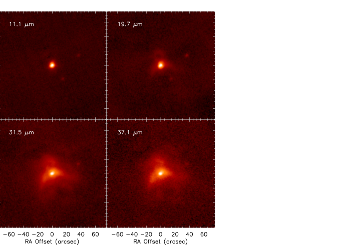
Figure 2: FORCAST images of MWC297 at 11, 19, 31, and 37 $\mu$m, displayed with asinh scaling (Lupton et al., 1999). North is up and East is left. The two Class II sources MWC 297#1 and #2 can be clearly seen at 11.1 and 19.7 $\mu$m.

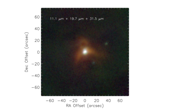
Figure 3: Three-color image generated by combining the FORCAST 11.1 (blue), 19.7 (green), and 31.5 (red) $\mu$m images.

Table 2: SOFIA/FORCAST Observations of MWC 297

Filter	Flight	UT Date	UT Time	$t_{exp}$	Altitude	Zenith Angle	$C$
($\mu$m)				(s)	(feet)	(deg)	(Me- s-1 Jy-1)
6.6	170	2014 May 08	11:12:29	120	42983	43.6	0.093 $\pm$ 0.004
11.1	170	2014 May 08	11:05:35	180	42973	44.0	0.363 $\pm$ 0.033
19.7	170	2014 May 08	10:58:49	189	42993	42.8	0.530 $\pm$ 0.012
31.5	170	2014 May 08	11:05:35	222	42973	44.0	0.165 $\pm$ 0.013
37.1	170	2014 May 08	10:58:49	429	42993	42.8	0.044 $\pm$ 0.004
11.1	178	2014 Jun 11	08:25:21	180	43001	43.6	0.354 $\pm$ 0.010
19.7	178	2014 Jun 11	08:12:15	208	42995	44.6	0.535 $\pm$ 0.016
31.5	178	2014 Jun 11	08:25:21	197	43001	43.6	0.106 $\pm$ 0.004
37.1	178	2014 Jun 11	08:12:15	199	42995	44.6	0.028 $\pm$ 0.003

Table 3: Positions and flux densities of FORCAST mid-infrared sources in the MWC 297 field

Source	$\alpha$(2000.0)	$\delta$(2000.0)	S(6.6 $\mu$m)	S(11.1 $\mu$m)	S(19.7 $\mu$m)	S(31.5 $\mu$m)	S(37.0 $\mu$m)
	[h m s]	[∘ ′ ′′]	[Jy]	[Jy]	[Jy]	[Jy]	[Jy]
MWC 297 core	18 27 39.53	$-$03 49 52.1	109.9 $\pm$ 4.8	118.8 $\pm$ 3.5	109.5 $\pm$ 3.4	113.9 $\pm$ 15.4	97.7 $\pm$ 18.6
#1	18 27 37.07	$-$03 49 38.5	0.88 $\pm$ 0.02	1.04 $\pm$ 0.01	1.47 $\pm$ 0.12	$\cdots$	$\cdots$
#2	18 27 38.55	$-$03 50 11.0	1.04 $\pm$ 0.01	0.93 $\pm$ 0.01	0.67 $\pm$ 0.07	$\cdots$	$\cdots$
#3	18 27 38.69	$-$03 49 54.1	0.43 $\pm$ 0.02	$<$ 0.06	$\cdots$	$\cdots$	$\cdots$
#4	18 28 38.17	$-$03 49 44.0	0.80 $\pm$ 0.02	0.34 $\pm$ 0.03	$\cdots$	$\cdots$	$\cdots$
#5	18 27 38.83	$-$03 49 34.8	0.61 $\pm$ 0.02	0.44 $\pm$ 0.03	$\cdots$	$\cdots$	$\cdots$
#6	18 27 38.95	$-$03 50 01.4	0.22 $\pm$ 0.03	$<$ 0.06	$\cdots$	$\cdots$	$\cdots$
MWC 297 extd	18 27 39.53	$-$03 49 52.1	111.4 $\pm$ 4.9	121.6 $\pm$ 3.6	171.6 $\pm$ 5.3	513.1 $\pm$ 18.5	650.4 $\pm$ 64.7

MWC 297 was observed with FORCAST on SOFIA as part of a cycle 2 project (02_0016) targeting disks around early B-stars. FORCAST is a dual-channel mid-infrared camera covering 5 - 40 $\mu$m with a suite of broad and narrow-band filters (Herter et al., 2012). Each channel consists of an array of 256 $\times$ 256 pixels. Both channels can be operated simultaneously via a dichroic mirror internal to FORCAST, which was the configuration used for these observations. MWC 297 was observed using the ‘Nod-Matched-Chop’ mode with dithering. On 08 May 2014, all observations were (erroneously) executed with a 30^′′ east-west chop throw and nod, using the filter combinations 19.7/37.1 $\mu$m, 11.1/31.5 $\mu$m, and 6.6/37.1 $\mu$m, resulting in twice the integration time for 37.1 $\mu$m. Unfortunately, because of the the large angular extent of the emission in MWC297, the relatively small chop/nod throw renders these images useful only for investigating point sources in the vicinity of MWC297. The observations were repeated on 11 June 2014 with a 270^′′ chop throw at a position angle of 320^∘, in the filter combinations 19.7/37.1 and 11.1/31.5 $\mu$m. These images are shown in Figure 2 and were used to measure the flux from MWC297 and for the subsequent analysis. On both flights MWC 297 was observed at an aircraft altitude of $\sim 43000$ feet with excellent sky transmission, although the sky background was somewhat variable on the second flight. Details of the observations are given in Table 2.

We retrieved the Level 3 data from the SOFIA Science archive. These pipeline reduced and calibrated images require no further processing; details about FORCAST data reduction and calibration can be found in Herter et al. (2013). The pixel size after pipeline processing is 0.768^′′. We found that the relative positions of the source were different in the various filters. We manually shifted the images such that the centroid of the peak of the emission in all the filter images was aligned with that seen in the 11.1 $\mu$m filter.

Figure 3 shows a three color image of MWC 297 generated from the 11.1, 19.7, and 31.5 $\mu$m filter images obtained during the second SOFIA flight. At wavelengths shorter than 19.7 $\mu$m, the images reveal only unresolved point sources, and the data from the first flight can also be used for point source photometry. At 6.6 $\mu$m we see six sources, three of which are new detections. All the new sources are within 20^′′  of MWC 297, which is severely saturated in Spitzer and WISE images. This makes it impossible to see even a moderately faint source in the vicinity of the star. At 11.1 $\mu$m and longer wavelengths only MWC 297 and the two brightest young stellar objects are visible. The latter two both have 2MASS counterparts and were first detected in the mid-infrared by Habart et al. (2003) at 10.5 $\mu$m. MWC 297#1 is also a sub-millimeter source, first detected by Henning et al. (1998) and is also visible in the SCUBA 850 and 450 $\mu$m images presented by Sandell, Weintraub & Hamidouche (2011). In Gutermuth et al. (2009), who observed the MWC 297 region with Spitzer IRAC and MIPS they are listed as MWC 297 #6 and #7. They characterize both as Class II objects.

Flux densities from PSF fitting or aperture photometry (using a radius of 12 pixels) of the central stellar core are presented in Table 3, along with measurements for the other point sources detected in the FORCAST images. As can be seen in Figures 2 and 3, at wavelengths longer than 11.1 $\mu$m, the emission from the envelope surrounding the central star in MWC297 is quite prominent. Since we expect that this emission arises from dust reprocessing the ultraviolet and optical light from the central source, we used a large aperture with a radius of $54$^′′(70 pixels) to measure the total flux from the extended MWC297 region (stellar core plus envelope) in these images.

2.3 Herschel PACS and SPIRE archival data

The MWC 297 field was observed twice in the guaranteed time Key Program the Herschel Gould Belt Survey (HGBS) (André et al., 2010; Bontemps et al., 2010; Könyves et al., 2010). On Operational Day (OD) 163 (2009-10-24) MWC 297 was observed in parallel mode with PACS (70/160 $\mu$m) and SPIRE. The field was observed with fast scanning (60^′′/sec) with an orthogonal scan, resulting in an approximately symmetric, but significantly broadened PSF due to the fast scan rate. The PACS 70 $\mu$m data were retrieved from the HGBS website. These data are part of the observations discussed in Bontemps et al. (2010) as well as in Könyves et al. (2010, 2015). We also retrieved the level 2.5 SPIRE data from the Herschel data archive. MWC 297 was observed on OD 522 (2010-10-18) with PACS (100/160 $\mu$m) with medium scan speed (20^′′ s^-1) with an orthogonal cross scan. The latter data set has much better image quality. Level 2.5 JScanam images processed with HIPE 12.1.0 were retrieved for both 100 $\mu$m and 160 $\mu$m from the Herschel data archive.

Even though there is extensive emission surrounding MWC 297 from the molecular cloud associated with it, the central star is clearly visible in the PACS images (Fig. 4). The emission from MWC 297 is particularly obvious in the PACS 100 $\mu$m image, which has the best spatial resolution ($\sim$ 6.7^′′) of the three PACS images we analyzed. This is shown in Figure 5, where we overlay the PACS 100 $\mu$m image on the FORCAST 31.5 $\mu$m image. However, the central source cannot be seen in the SPIRE images, which are completely dominated by the molecular cloud emission (see Fig. 6). Note that the brightest source in the PACS 100 and 160 $\mu$m images and the SPIRE images is not the central star in MWC297, but rather a source about $20$^′′  to the northeast, which we refer to as the NE core. This object sits on the edge of the diagonal dust ridge and seems to be encircled by a faint blue halo. It can be clearly seen in the 450 and 850 $\mu$m maps shown by Alonso-Albi et al. (2009) and Sandell, Weintraub & Hamidouche (2011). We also detect MWC 297#1 at 100 $\mu$m and at 160 $\mu$m, but here the source is too blended with emission from the surrounding cloud to allow us to determine a reliable flux density. MWC 297#1 is not detected at 70 $\mu$m.

A three-color image generated by combining the PACS 70, 100, and 160 $\mu$m data is shown in Figure 4. In addition to measuring the flux from the central source in the three PACS bands, we also used a large aperture with a radius of $384$^′′(120 pixels) in order to capture all of the flux from the envelope surrounding the central star, which is expected to be reprocessed light from the central star. A similar sized aperture was used to estimate the fluxes in the SPIRE images. The fluxes are given in Table 4.

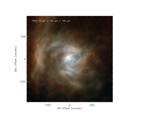
Figure 4: Three-color image of of MWC 297, generated from the PACS 70 (blue), 100 (green), and 160 (red) $\mu$m data on an asinh scale, of the region used to estimate total MIR fluxes. The arc detected in the SOFIA/FORCAST images, as well as the NE core, offset by about 15 ^′′from the center of MWC297, can be clearly seen. The arc is blue while the NE core is considerably redder. A faint blue halo can also be seen centered on the NE core. The dust ridge separating the central star in MWC297 from the NE core can also be seen.

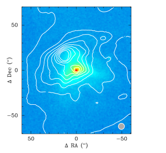
Figure 5: PACS 100 $\mu$m image (contours) overlaid on a logarithmically stretched FORCAST 31.5 $\mu$m image in color.

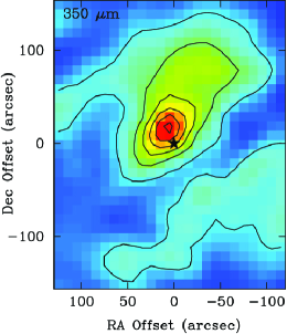
Figure 6: The 350 $\mu$m SPIRE image shows that MWC 297 is located on the southwestern rim of a small cloud. The emission at 350 $\mu$m is dominated by a prestellar core about 15^′′ northeast of the star. The gap to the southwest of the star is also seen in the ¹³CO(1 – 0) image by Ridge et al. (2003)

Table 4: Positions and flux densities of Herschel PACS sources in the vicinity of MWC 297.

Name	$\alpha$(2000.0)	$\delta$(2000.0)	S(70 $\mu$m)	S(100 $\mu$m)	S(160 $\mu$m)	comment
	[h m s]	[∘ ′ ′′]	[Jy]	[Jy]	[Jy]
MWC 297 core	18 27 39.51	$-$03 49 51.0	17.8 $\pm$ 5.0	16.3 $\pm$ 3.3	7.0 $\pm$ 3.0
MWC 297#1	18 27 37.31	$-$03 49 38.7	$\cdots$	1.8 $\pm$ 0.3	$\cdots$
NE Core	18 27 40.56	$-$03 49 34.7	51.7 $\pm$ 15.5	77.4 $\pm$ 8.0	45.6 $\pm$ 5.0	[KAM2015]68
MWC 297 extd	18 27 39.51	$-$03 49 51.0	4838 $\pm$ 160	6557 $\pm$ 230	6142 $\pm$ 441

2.4 BIMA observations

Observations of MWC 297 were conducted on several occasions between 2002 October and 2003 February at several frequencies and antenna configurations; see Table 5. The mm-emission is unresolved in all observations with the possible exception of the B-array data obtained on 2003 February 18. Therefore the synthesized beam size is not listed in Table 2 except for these 2003 February data. All data sets were reduced and imaged in a standard way using MIRIAD (Sault, Teuben & Wright, 1995). The quasar 1751$+$096 was used for phase calibration, 3C454.3 was used for amplitude calibration, and Uranus or MWC 349 was used for flux calibration. Since the primary objective of these observations was to characterize the continuum emission from MWC 297, the correlator was configured for four 100 MHz bands, except for the 110 GHz observations where ¹³CO(1–0) was centered in a 25 MHz wide window, while the other three correlator windows were set to 100 MHz. Figure 7 shows the B-array image with the integrated ¹³CO(1–0) emission in color overlaid with continuum emission in contours.

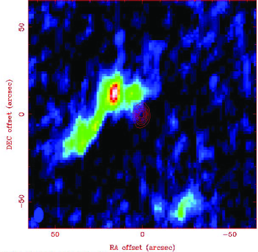
Figure 7: Integrated ¹³CO(1–0) emission plotted in color with 110 GHz continuum emission overlaid with red contours

Table 5: BIMA flux densities of MWC 297

Frequency	Flux density	Observing date(s)	Array configuration
[GHz]	[mJy]
075	85 $\pm$ 0.15	2002 Nov 29	C
107	149.6 $\pm$ 0.08	2002 Oct 28	C
108.5	146.25 $\pm$ 0.11	2003 Feb 17	B
230	340 $\pm$ 0.15	2002 Nov 26, 29	C

2.5 VLA observations and VLA archival data

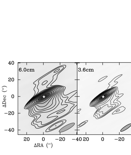
Figure 8: Re-reduced VLA CnD observations at 6.0 and 3.6 cm. The beam, which is very elliptical, is drawn in the right bottom corner of each image.

MWC 297 was observed with the VLA on 2003 December 5 in the C (4.89 GHz) and U-band (14.94 GHz) for 4.5 hrs in the B-configuration. The observing conditions were excellent and we had good UV coverage, giving a synthesized beam of 1.55^′′ $\times$ 1.15^′′ with a PA $=-22.1$^∘  in C-band and 0.49^′′ $\times$ 0.40^′′  with a PA $=-15.1$^∘ in U-band. 3C 286 was used for absolute calibration and 1832$-$105 for phase calibration. The data were reduced with AIPS in a standard way. MWC 297 was bright enough for self calibration, but the phase stability was so good that we could see no improvement in signal to noise with this option. We resolved the radio emission at both frequencies; see Table 6.

We searched the VLA archive and found a set of observations from 1978 December 9 - 10 (L and C band), which we retrieved, reduced, calibrated and created cleaned images at both frequencies. At the time VLA had only 9 antennas working, mostly on the east and the west arms. The bandwidth was 12.5 MHz and data were recorded for both R and L polarization. The maximum antenna spacing was 14.4 km, which places the antenna configuration somewhere between A and B. At L-band (1.48 GHz) the emission is extended with an integrated flux density of 8.8 $\pm$ 2.0 mJy. The C-band observations had better phase stability than the L-band observations and resulted in an rms noise of 0.4 mJy beam^-1 with a synthesized beam width of 3$\farcs$62 $\times$ 2$\farcs$21 and a PA = $-$19^∘. We find MWC 297 unresolved with a total flux density of 5.1 $\pm$ 0.4 mJy, which agrees quite well with our results from 2003, see Table 6.

Our observed flux densities agree quite well with those of Skinner, Brown, & Stewart (1993), except for their CnD (low spatial resolution) observations from 1991 Feb 7. We retrieved the latter data set from the VLA archive and re-reduced the data. The higher flux densities in the CnD data results from the inclusion of the bipolar ionized outflow lobes from MWC 297 (Fig. 8, which are filtered out in in the A and B-array data. Performing a careful two-component Gaussian fit (one for the compact core and one for the extended emission), we find very consistent results for the core emission (see Table 6 and Skinner, Brown, & Stewart 1993). The flux densities for the outflow lobes were estimated by integrating over the role are of emission and subtracting out the flux densities for the compact core. The CnD observation also included L-band (1.49 GHz) observations of the MWC 297 field. Here the emission is dominated by the outflow lobes and an estimate of the flux of the compact core could not be obtained. The total flux density flux at 1.49 GHz (core + outflow lobes) is 15.3 $\pm$ 2.1 mJy.

Table 6: VLA data on MWC 297

Frequency	Core size	PA	rms	Flux Density
				Peak	Core Total	Outflow Lobes
[GHz]	′′ $\times$ ′′	[deg]	[mJy beam-1]	[mJy]	[mJy]	[mJy]
4.86	$\cdots$	$\cdots$	0.074	07.04 $\pm$ 0.07	7.48 $\pm$ 0.01	8.6
4.89	0.33 $\times$ 0.15	0$-$90 $\pm$ 12	0.034	06.18 $\pm$ 0.03	6.56 $\pm$ 0.06	$\cdots$
4.90	1.3 $\times$ 0.8	0$+$160 $\pm$ 18	0.170	5.1 $\pm$ 0.4	5.1 $\pm$ 0.4	$\cdots$
8.44	$\cdots$	$\cdots$	0.052	10.67 $\pm$ 0.05	10.82 $\pm$ 0.10	5.2
8.44	$\cdots$	$\cdots$	0.046	6.35 $\pm$ 0.06	8.88 $\pm$ 0.10	$\cdots$
8.44	$\cdots$	$\cdots$	0.046	6.19 $\pm$ 0.07	8.80 $\pm$ 0.10	$\cdots$
14.93	0.14 $\times$ 0.11	0$+$26 $\pm$ 16	0.067	17.79 $\pm$ 0.07	19.62 $\pm$ 0.12	$\cdots$

3 Results

3.1 Morphology

The Herschel PACS and SPIRE images show that MWC 297 lies on the southeastern rim of a ridge with a more extended cloud core north of the star. There is a gap or low density area parallel to the ridge seemingly splitting the cloud into a northern and a southern or southwestern core, the latter being less dense (Figure 6). The same structure is also seen in the SCUBA-2 images Rumble et al. (2015), although the cloud to the southwest is rather faint. Maps of ¹³CO J = 1– 0 and C¹⁸O J = 1– 0 (Ridge et al., 2003) show the same southeastern ridge as seen in the PACS images, including the cloud southwest of MWC 297. The ¹³CO map shows that there is essentially a cavity southwest of the ridge splitting the clouds in two. In the sub-millimeter images one can see a protostellar core northeast of the star, which starts to dominate the emission shortward of 850 $\mu$m. At 350 $\mu$m it is very bright and MWC 297 is no longer visible. This core is also associated with strong ¹³CO emission seen in the BIMA image (Figure 7).

The VLA data obtained by Skinner, Brown, & Stewart (1993), and re-reduced by Sandell, Weintraub & Hamidouche (2011), in the CnD configuration show that MWC 297 powers a large bipolar ionized jet (see also Rumble et al., 2015), or outflow, oriented approximately north-south. In the south the outflow has a wide opening angle, while in the north it appears much weaker and narrower. The thermal emission is dominated by a compact core, centered on the star, with a spectral index, $\alpha\sim$ 1.03 and a size decreasing with increasing frequency, as typically seen in collimated thermal jets (Reynolds, 1986; Sandell et al., 2009). Sub-arcsecond imaging at 5 GHz (Drew et al., 1997) resolves the core into a double peaked east-west structure (presumably the ionized disk) with a more pronounced north-south extension in the outflow direction.

In the MIR, at wavelengths $\lambda<19\mu$m, MWC 297 appears as an unresolved, point-like source in the FORCAST images. However, at longer MIR wavelengths, the source is clearly extended. An wide arc, opening to the southwest, whose tips are separated by $\sim 32$^′′($\sim 13400$ au), is clearly seen in the 19, 31, and 35 $\mu$m images. The arms of the arc extend about $\sim 14-18$^′′(5850 - 7520 au) from the central source. A small loop, or annulus, with a diameter of $\sim 10$^′′(4180 au), can be seen to the northeast in the 19 and 31 $\mu$m images. The annulus and arc are very nearly symmetric with respect to the central source, with the arc opening in nearly the opposite direction to the position of the northern annulus.

The structure seen in the long wavelength FORCAST images mirrors that seen in the VLA data. A comparison between the FORCAST 31 $\mu$m image and the VLA 6 cm map is shown in Figure 9. These data suggest that the ionized outflow from MWC 297 is surrounded by a warm dust layer, which is perhaps being compressed and heated in the shear layer between the outflow and the surrounding molecular cloud. The compact nature of the emission to the north indicates the the outflow is constrained by the dense environment in this direction. Therefore, we interpret the arc and the northern loop seen in the FORCAST images as arising from dust on a bi-conical surface, surrounding the outflow, that is tipped with respect to the line of sight; the southwestern arc traces the edge-brightened surface that is tipped toward us and the northeastern annulus traces the circular rim of the northern structure that is tipped away from us. Diagrams of similar outflow structures can be seen in the papers by Cantó et al. (1981); Raga et al. (1993).

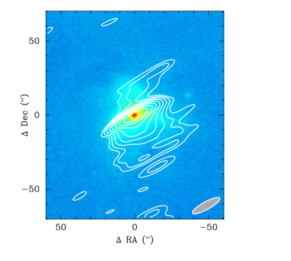
Figure 9: VLA 6 cm image (contours) overlaid on a logarithmically stretched FORCAST 31.5 $\mu$m image in color. The VLA beam is plotted at bottom right.

In order to determine the properties of the dust in the southwestern arc and northern loop, we estimated the dust temperature at each pixel in the 19.7, 31.5, and 37.1 $\mu$m combined image by fitting the emission with a model given by

$$F_{\nu}=\Omega\cdot S_{\nu}(T_{dust})\cdot[1-\exp(-\tau_{\nu})]$$ (1)

where $S_{\nu}(T)$ is the blackbody function, $T_{dust}$ is the temperature of the dust, and $\tau_{\nu}$ is the dust opacity (see e.g. Shuping et al., 2012). We adopted the dust opacity law of McClure (2009). Note that the full-width at half maximum (FWHM) of the point spread function (PSF) in the FORCAST images does not vary substantially across this wavelength range. The resulting dust map and radial profile are presented in Fig. 10. The temperature map indicates that the dust has a relatively uniform temperature of $T_{dust}\sim 67$K and a low optical depth ($\tau_{\nu}<<1$) at all of the FORCAST wavelengths.

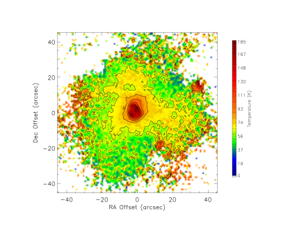
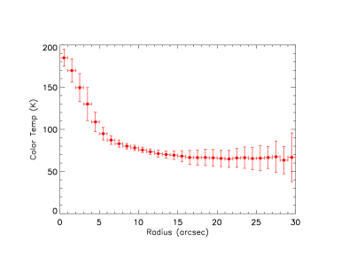
Figure 10: (left) Dust temperature map derived from the FORCAST data. The contour around the bright yellow/orange region in the map corresponds to $T\approx 67$ K. (right) Azimuthally averaged radial profile of the dust temperature.

3.2 System Inclination

To constrain the inclination of the system, we constructed a simple geometrical model of the outflow structure and synthesized MIR images which could be compared to the FORCAST data. For simplicity, we limited ourselves to modeling only the southwestern arc , for which the FORCAST images provide sufficient data to constrain any models. We assumed that the dust emission traced the surface of a conical outflow with a shape given by $r(z)\sim z^{\alpha}$. The dust emission surface was assumed to be physically and optically thin, with a uniform thickness, and isothermal with a temperature of 67 K; these assumptions are justified by our results described above. In order to simulate the wavelength dependence of the dust emission, we assumed a wavelength dependence of the dust emissivity of $Q_{abs}\sim\lambda^{-1.5}$. The dust emission spectrum was scaled to roughly match the observed surface brightness in the FORCAST images. The central source was added to the image, with an intensity at each wavelength equal to that seen in the FORCAST images. The simulated images were scaled to match the observed physical size of the FORCAST images. We rotated the structure in three dimensions, convolved the resulting image with a Gaussian with a FWHM equivalent to that of the FORCAST PSF (FWHM $\sim 3^{\prime\prime}$), and resampled it to match the FORCAST pixel size. The free parameters of the model were the power law index of the conical shape, $\alpha$, the position angle (PA) on the sky, and the inclination angle, $i$. We generated $\sim 800$ models with a range of parameter values ($\alpha$ was varied between 0.1 and 0.6, $i$ between 35 and $60$^∘, and PA between 185 and $210$^∘) and attempted to match the resulting image to the observations. The best-fit parameters, yielding an image most similar to that of the data, were found to be $\alpha=0.3\pm 0.15$, PA $=197\pm 10$^∘, and $i=55\pm 5$^∘. Given the limited length of the arc seen in the FORCAST images and the relatively low signal-to-noise ratio and contrast of the emission compared to the background, the uncertainties on $\alpha$ and the PA are fairly large and a wide range of values provided reasonable fits to the data. However, the PA we find agrees well with that determined by Sallum et al. (2021) from interferometric imaging with the LBT. Furthermore, the inclination of the conical structure is quite well-constrained. The synthetic image produced by the model for these parameters shown in Fig. 11 is remarkably close to the observations. We then used the same model to generate synthetic images using the parameters derived from the analyses of the NIR interferometric data (PA $\sim 56$^∘, and $i\sim 15$^∘from Malbet et al. 2007; PA $\sim 120$^∘, and $i\sim 40$^∘from Acke et al. 2008), with $\alpha\sim 0.3$. The resulting synthetic images are shown in Fig.11, which demonstrates that these parameters cannot reproduce the structure seen in the FORCAST images.

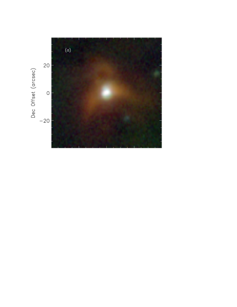
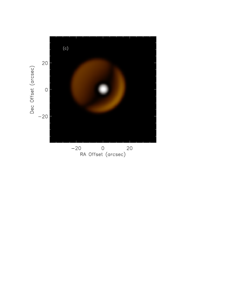
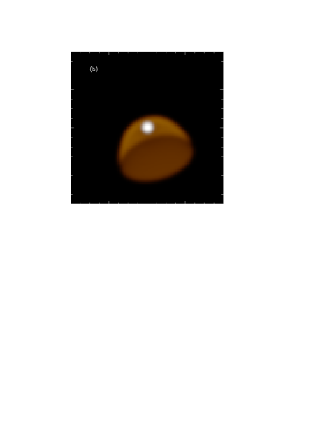
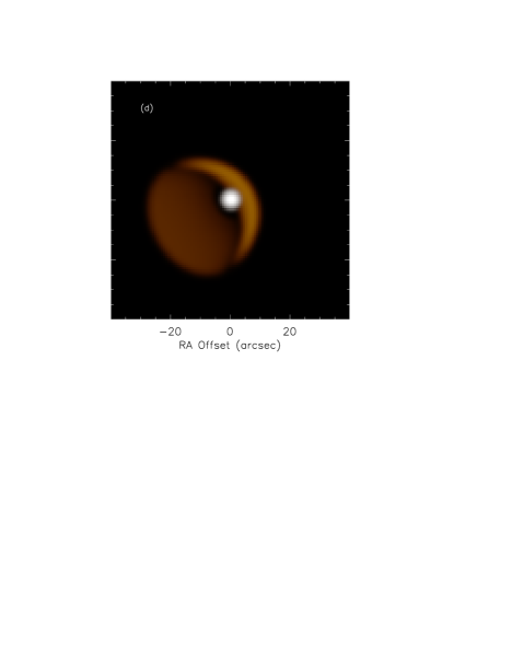
Figure 11: (a) Center of the FORCAST 3-color image on an asinh intensity scale; (b) Simulated image for best fit parameters found in this work (PA $=197$^∘and $i=55$^∘) on the same intensity scale; (c) Simulated image generated for PA $\sim 56$^∘and $i\sim 15$^∘, as found by Malbet et al. (2007); (d) Simulated image generated for PA $\sim 120$^∘and $i\sim 40$^∘, as found by Acke et al. (2008).

3.3 Outflow Parameters

The IRTF spectrum reveals strong emission lines from the H Paschen, Brackett, and Pfund series, as well as O I lines, atop a strong, red continuum. The He I 1.083 $\mu$m line can be seen and exhibits a clear P Cygni profile, with two absorption dips. Weak CO 2-0 bandhead emission can be seen at 2.29 $\mu$m. Continuum discontinuities associated with the three H line series are quite prominent and are clearly in emission. There is no evidence of any absorption lines associated with the stellar photosphere, which indicates that the near-infrared continuum at wavelengths at least as short as 0.8 $\mu$m is dominated by a combination of dust, bound-free, and possibly free-free continuum emission.

The large number of H lines in the spectrum provides a wealth of data that can be used to infer the properties of the system. We detect at least 57 H lines in the Paschen (down to the Pa 25 line), Brackett (to Br 30), and Pfund (to Pf 34) series, along with lines of He I and O I, with a signal-to-noise ratio considerably higher than in the spectra of Benedettini et al. (2001). As shown in Fig 12, the line fluxes and flux ratios estimated from the standard Case B assumption (Storey & Hummer, 1995) do not provide a good fit to the entire set of observed values for any values of temperature and electron density (see also Drew et al., 1997; Benedettini et al., 1998). Following Nisini et al. (1995) and Benedettini et al. (2001), we therefore constructed wind models, using the Sobolev approximation (Sobolev, 1960) and the formalism developed by Castor (1970), to predict the strengths of hydrogen emission lines under the assumption of a two-level atom (see e.g., Peraiah, 2002, chap. 9). The models assume that the wind is isothermal and fully ionized and that LTE conditions apply. An extensive discussion of the applicability and limitations of these assumptions for wind models of HAeBe stars is given by Nisini et al. (1995). The assumed velocity profile is given by

$$v(r)=v_{i}+(v_{max}-v_{i})\Bigg{(}1-\bigg{(}\frac{r_{i}}{r}\bigg{)}^{\alpha}\Bigg{)}$$ (2)

where $v_{i}$ is the velocity at the base of the wind, located at $r_{i}$, and $v_{max}$ is the terminal velocity of the wind. This expression for the velocity profile is commonly used in the analysis of hot star winds (see Groenewegen & Lamers, 1989). The mass loss rate $\dot{M}$ for the wind is then given by

$$\dot{M}=4\pi r^{2}m_{p}n_{e}(r)v(r)~{}.$$ (3)

We did not incorporate variations with wind velocity and mass flux with stellar latitude (Malbet et al., 2007). In these models, the flux density at a frequency $\nu$ arising from a line transition at frequency $\nu_{0}$, with statistical weight of the lower level $g_{l}=2l^{2}$, oscillator strength $f_{lu}$, and energy of the lower level of $E_{l}=13.6/l^{2}$, is given by

$$F_{\nu}=\frac{2\pi S_{\nu}(T)}{D^{2}}\int_{r_{i}}^{r_{o}}(1+\mu^{2}(\nu,r)\sigma(r))[1-\exp(-\tau(\mu,\nu,r))]rdr$$ (4)

where $S_{\nu}(T)$ is the Planck function at temperature $T$, which we have assumed is constant throughout the wind. Here $\mu$ is the angle between the radial direction and the line of sight and is given by

$$\mu=\frac{c}{v(r)}\frac{\nu-\nu_{0}}{\nu_{0}},$$ (5)

while

$$\sigma(r)=\frac{r}{v(r)}\frac{dv}{dr}-1$$ (6)

and

$$\tau(\mu,\nu,r)=\frac{\tau_{0}(r)}{1+\mu^{2}(\nu,r)\sigma(r)}$$ (7)

where

$$\begin{split}\tau_{0}(r)=\frac{\pi e^{2}n_{e}^{2}r}{2m_{e}v(r)\nu_{0}}\Bigg{(}\frac{h^{2}}{2\pi m_{e}kT}\Bigg{)}^{1.5}g_{l}f_{lu}\exp(E_{l}/kT)[1-\exp(-h\nu_{0}/kT)]\end{split}$$ (8)

To keep the number of free parameters relatively small, we assumed $D=418$ pc, $T=10000$ K, $v_{i}=20$ km s^-1 (in agreement with Nisini et al., 1995 and Benedettini et al., 2001) and $\alpha=1$ (in agreement with the description of the winds for massive stars; Puls et al., 1996, e. g.). Although we explored models with a variety of values for $r_{i}$, we decided to adopt $r_{i}=R_{\star}=6R_{\odot}$. This left us with $\dot{M}$, $v_{max}$, and $\rho=r_{o}/r_{i}$ as the free parameters. Based on the observed line widths (mean FWHM $\sim 200$ km s^-1) and the inherent resolution of the instrument ($R\sim 2000$), we limited $v_{max}$ to be less than or equal to 200 km s^-1.

Table 7: Adopted Values for Wind Model Parameters

Parameter	Values	Units
$\alpha$	0.0, 1.0
$v_{max}$	50, 75, 100, 150, 200	km s-1
$\dot{M}$	$5\times 10^{-8}$, $(1,3,5,5.5,6,6.5,7,7.5,8,8.5,9,9.5)\times 10^{-7}$, $(1,1.1,2,3)\times 10^{-6}$	$M_{\odot}$ yr-1
$\rho$	2, 5, 10, 15, 20, 25, 30, 35, 40, 45, 50, 75, 100, 125, 150, 200
$A_{V}$	4 - 12 in steps of 0.1	mag

We generated over $1300$ models with a range of parameter values centered on those found by (Benedettini et al., 2001); the range of values adopted for the various parameters are given in Table 7. For each model we computed the fluxes of the H lines of the Paschen, Brackett, and Pfund series up to at least $n_{\rm upp}=30$. We then reddened the line fluxes using the Cardelli, Clayton & Mathis (1989) extinction model and $A_{V}$ values between 4 and 12 mag in steps of 0.1 mag. This resulted in over $10^{5}$ reddened models. We compared these reddened models with the observed line fluxes and determined the best fitting model by computing $\chi^{2}$. We found that the best fit to the observed line strengths were provided by the model with $\rho\geq 200$, $v_{max}=50$ km s^-1, $\dot{M}=6.0\times 10^{-7}M_{\odot}~{}\mathrm{yr}^{-1}$ and $A_{V}=8.1$ mag. A comparison between the observed line fluxes and those of the best fit model are shown in Fig 12. The model spectrum, convolved to the SpeX resolution ($R\approx 2000$), is plotted along with our continuum-subtracted SpeX spectrum in Fig. 13. The latter figure indicates that the model provides a very good match for most of the observed lines, although it slightly underestimates the strength of the Pa $\beta$ line (in contrast to the results of Nisini et al. 1995) and overestimates the flux of the highest and lowest Br transitions. All of the lines, even those arising from high upper levels, are found to be optically thick. The radial profiles of the wind velocity and the electron density in the wind, computed with our best fit parameters are shown in Figure 14. Based on the $\chi^{2}$ fits, we estimate the the allowed ranges on the reddening and mass-loss values to be $A_{V}=8.1\pm^{2.5}_{1.5}$ mag and $\dot{M}=6.0\pm^{3.7}_{1.7}\times 10^{-7}M_{\odot}~{}\mathrm{yr}^{-1}$. Due to our model sampling, useful constraints cannot be derived for $v_{max}$ although the derived value is consistent with the observed widths of the strongest emission lines in the SpeX spectrum. Constraints on $\rho$ are also difficult to obtain, as almost all values of $\rho>25$ yielded acceptable fits. Models with $\rho$ values up to as large as 2000 were generated and slightly better fits to the observed spectrum were found as $\rho$ increased, although the improvement was minuscule and almost entirely due to a tiny increase in the predicted Pa $\beta$ line flux. On the other hand, we can estimate the radius of the line emitting region by assuming that this radius represents the surface at which $\tau=1$, and the line emission is given by a blackbody with temperature $T$ (see Nisini et al., 2004). In this case,

$$r_{o}=\Bigl{[}\frac{cL_{\rm line}}{4\pi^{2}B_{\lambda}(\lambda,T)\lambda\Delta v}\Bigr{]}^{0.5}~{}~{}~{},$$ (9)

where $L_{line}$ is the luminosity in the line, and $B_{\lambda}(\lambda,T)$ is the Planck function. For both Pa $\beta$ and Br $\gamma$, with $T=10000$ K, and $\Delta v=50$ km s^-1 we find $r_{o}\lesssim 1$ au, or $\rho\lesssim 30$. The best fit value of $\rho=200$ corresponds to $r_{o}=5.6$ au.

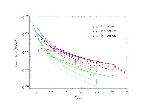
Figure 12: Comparison between observed line fluxes and those predicted by the wind model (solid lines) as a function of the upper level number for the transition $n_{\rm upp}$. Solid symbols denote measurements from the IRTF/SpeX data, while open symbols are from Benedettini et al. (2001). Dotted lines are Case B values for $T=10000$ K, $n_{e}=1.0\times 10^{2}$ cm^-3, reddened by $A_{V}=8.1$ mag and scaled to match the observed Pa $\beta$ flux, while the dashed lines are similarly Case B values for $n_{e}=1.0\times 10^{10}$ cm^-3.

Figure 13: Comparison between the continuum-subtracted IRTF/SpeX spectrum and the best fitting wind model (red). Only H lines have been synthesized in the model.

Figure 14: Radial profile of the electron density (left hand scale) and wind velocity (right hand scale) in H line emitting region for our best fit parameters and the adopted wind model.

Our estimate of the reddening is in good agreement with the values found in the literature (e.g. Nisini et al., 1995; Drew et al., 1997; Benedettini et al., 2001; Fairlamb et al., 2015; Vioque et al., 2018; Ubeira-Gabellini et al., 2020; Wichittanakom et al., 2020). Furthermore, the value of $v_{max}$ we find is consistent with that found by Drew et al. (1997) for the Br$\alpha$ line, although it is significantly smaller than the value adopted by Nisini et al. (1995) based on the width of the H $\alpha$ line in the spectrum shown by Finkenzeller & Mundt (1984). Their value of 380 km s^-1is not supported by the observed widths of the emission lines in our spectrum. The mass-loss rate derived from our best fit model is about 30% of the value found by Benedettini et al. (2001) and about half that given by Nisini et al. (1995) (both for a distance of 450 pc), while our reddening estimate is only slightly larger. This is perhaps unsurprising given that variations in the widths and strengths of the strongest H lines in MWC 297 have been reported in the literature (see e.g. Drew et al., 1997; Benedettini et al., 2001; Eisner et al., 2015). Our measured line strength for the Pa $\beta$ line is about half that given by Nisini et al. (1995) while our Br $\gamma$ line flux is about 16% larger. We note that our mass-loss rate is about a factor 5 smaller than that derived by Jinliang et al. (1997) using non-LTE wind models and the line fluxes reported by Nisini et al. (1995).

The tendency of the wind models to overestimate the strengths of the weakest transitions (i.e., those with the highest upper levels, $n_{\rm upp}$) was before noted by Nisini et al. (2004), who suggested that this may indicate that the wind velocity law is incorrect. While a much steeper acceleration, occurring over a much smaller radius, may possibly yield better fits, such a velocity law seems unphysical and is inconsistent with the description of winds from massive stars. While a full investigation of the wind velocity law is beyond the scope of this paper, we did generate a set of models with $\alpha=0$, and a smaller set with $\alpha=10$, as extreme examples of a wind that is at, or close to, the terminal velocity when it leaves the stellar surface. We did not find that these models produced significantly better fits to the data than those with $\alpha=1.0$; better fits to the strengths of the weaker lines in each series were obtained at the expense of poorer fits to the lines with intermediate values of $n_{\rm upp}$. Significantly, we also found that the parameters of the best fit model to the observed line fluxes were very similar to those we found above ($\dot{M}=8.5\times 10^{-7}M_{\odot}~{}\mathrm{yr}^{-1}$, $A_{V}=8.2$ mag, $v_{max}=75$ km s^-1, and $\rho=200$).

The H line strengths provide an estimate of the ionizing luminosity. If the lines were optically thin, we could use the predicted emissivities tabulated by Storey & Hummer (1995) for Case B conditions to estimate the ionizing luminosity producing the H lines. Adopting a gas temperature of $10^{4}$ K and an electron density of $10^{9}$ cm^-3, using the observed strengths of the Br $\gamma$ lines, correcting for extinction corresponding to $A_{V}=8.1$ mag, and adopting a distance of 418 pc, we find the ionizing photon flux to be $Q_{0}\sim 2\times 10^{47}$ photons s^-1. Of course, our models indicate that none of the H lines are optically thin, and therefore the Case B estimate of $Q_{0}$ is not strictly applicable, but it can be considered a lower limit to the true ionizing flux in the system. We can also use the equation from Felli & Panagia (1981) to estimate the ionization rate for an accelerating wind for a given mass-loss rate. For the mass-loss rate we find from our models, and the velocity law we have adopted, we find $Q_{0}=2.2\times 10^{48}$ photons s^-1. Using a Kurucz model with a temperature of 24000 K, a $\log g$ of 4.0, and a radius of $6R_{\odot}$, parameters typical of a B1.5 V star (Bohm-Vitense, 1981; SchmidtKaler, 1982), we estimate the ionizing photon flux generated by the star to be $Q_{0}=3.8\times 10^{45}$ photons s^-1, a factor of at least $50$ smaller than the estimated value. A similar, but slightly smaller, value of $2.9\times 10^{45}$ photons s^-1 is found using the B star models of Lanz & Hubeny (2007). With our assumed velocity law, the maximum mass-loss rate for which a B1.5V star can completely ionize its wind is only $\sim 2.5\times 10^{-8}M_{\odot}~{}\mathrm{yr}^{-1}$ (see Felli & Panagia 1981), clearly far below the value we estimate from the emission lines in our SpeX data. This result suggests that either the wind is completely ionized within only a tiny region beyond the stellar photosphere (which seems incompatible with our model results) or nearly all of the ionizing luminosity is generated by the accretion process (e.g., by shocks, as the accreting material impacts the stellar surface), not the star itself.

The Br $\gamma$ luminosity is often used as a measure of the accretion rate of a young stellar object. In the case of MWC 297, our dereddened luminosity is $L({\rm Br}\gamma)/L_{\odot}\approx 0.67$. Using the correlation between $L({\rm Br}\gamma)$ and the accretion luminosity $L_{acc}$ given by Fairlamb et al. (2015), we find $L_{acc}\approx 1.7\times 10^{4}L_{\odot}$, which in turn corresponds to a mass accretion rate of ${\dot{M}}_{acc}\approx 3.3\times 10^{-4}M_{\odot}$ yr^-1, or about 540 times larger than the mass-loss rate we derive from our wind models. If we use the observed Pa $\beta$ line strength, we estimate $L_{acc}\approx 3.2\times 10^{4}L_{\odot}$ and ${\dot{M}}_{acc}\approx 6.2\times 10^{-4}M_{\odot}$ yr^-1, nearly a factor of two larger. Such large accretion rates accord with our observation of an optical and NIR continuum dominated by emission lines and bound-free continuum, with the Paschen, Brackett, and Pfund jumps all in emission. The accretion rate we derive from the Br $\gamma$ luminosity is in good agreement with the value estimated by Wichittanakom et al. (2020) from the H $\alpha$ line strength. However, it is a factor of $\sim 9$ times larger than that given by Guzman-Diaz et al. (2021) and $\sim 8$ times larger than that derived by Fairlamb et al. (2015) (after accounting for the different distance adopted).

3.4 SED

To generate the spectral flux and spectral energy density (SED) of MWC 297, we began by compiling and carefully examining the data in the voluminous literature on this object, using the table in Appendix A.9 of Alonso-Albi et al. (2009) as an initial guide. In addition to our SOFIA/FORCAST, Herschel/PACS, and Herschel/SPIRE measurements, we included photometry from a number of individual measurements reported in the literature as well as sky surveys, including Pan-STARRS (Chambers et al., 2016), GAIA (Riello et al., 2021), APASS (Henden et al., 2015), SkyMapper (Wolf et al., 2018), TASS (Richmond et al., 2000), FONAC-S (Yuldoshev et al., 2017), DENIS (Kimeswenger et al., 2004), 2MASS, IRAS, and MSX. Filter wavelengths were adopted from the various references or, in the case of the Johnson/Cousins system, computed using the response functions given by Mann & von Braun (2015). Similarly, magnitudes were converted to fluxes in Jy using the zero points in the references or from Mann & von Braun (2015). We then added our own submm/radio measurements, as well as those of Skinner, Brown, & Stewart (1993), Mannings (1994), Henning et al. (1998), Manoj et al. (2007), and Alonso-Albi et al. (2009). If multiple measurements at the same wavelength were available, we computed a weighted average. The full list of adopted fluxes is given in Table8.

In Figure 15 we present the full spectral energy distribution of MWC 297 from 0.36 $\mu$m to $6.0$ cm. We included the archival ISO spectrum and our SpeX spectrum (scaled by a factor of 1.22) in the plot. Values that were used to generate averages are plotted in light blue. Dashed lines connect photometric measurements for the core and and core+extended emission at the same wavelength. This figure demonstrates the remarkable agreement between the flux levels of the various data sets, at least in the NIR and beyond, including the SOFIA photometry. At wavelengths longwards of 20 $\mu$m the ISO spectrum deviates from the other measurements because the rectangular ISO aperture captured only a fraction of the total flux in the extended envelope.

The flux for a Kurucz model with $T_{eff}=24000$K, $\log g=4.0$, and $R=6R_{\odot}$, corresponding to parameters for a B1.5V star, at a distance of 418 pc and reddened by $A_{V}=8.1$ mag, is also shown in Figure 15. The fluxes for this stellar model are well below the optical photometry points. A good fit to the optical photometry can be obtained if the reddening is reduced ($A_{V}\sim 7$ mag) or the stellar radius is increased ($R\sim 10R_{\odot}$). Radius values larger than $10R_{\odot}$ yield model spectra that are incompatible with the blue end of our SpeX spectrum while models with radii larger than $\sim 7R_{\odot}$ are incompatible with the critical rotation velocity (see Section 4.1). Irrespective of the specific parameter values, it is clear from both this figure and our SpeX spectrum (Fig. 1) that the flux longwards of about 0.8 $\mu$m is dominated by continuum emission that is not from the stellar photosphere, but must be generated by the accretion process.

To estimate the total luminosity, we fit a smooth curve to the photometric points shown in Figure 15 and integrated under the curve between 0.35 and $6.0$ cm. We find that the core of MWC297 generates a luminosity of approximately $740~{}L_{\odot}$, far below that expected for an early B star ($\sim 1.1\times 10^{4}L_{\odot}$). Including the flux from the extended emission region, under the assumption that this represents re-processed UV emission arising from dust which has been heated by MWC 297, we find a total luminosity of only $\sim 2300~{}L_{\odot}$. If MWC297 is an early B star, then clearly the dust that provides the optical reddening is not the same dust that is re-processing the UV flux from the star and re-radiating it in the infrared. If, instead, we assume that the reddening is produced by dust along the line of sight, but distant from MWC297, as suggested by Acke et al. (2008), then we should correct the optical and near-infrared photometry for this absorption before integrating to estimate the total luminosity. Adopting $A_{V}=8.1$ mag, we find that the dereddened core of MWC 297 produces a total luminosity of about $5300~{}L_{\odot}$. Including the emission from the extended region yields a total luminosity of about $6900~{}L_{\odot}$, still somewhat below what one would expect from a B1.5V star. Of course, we are missing the flux emitted between the UV and the optical $U$ band which could account for some of the difference. For the Kurucz model, the luminosity emitted between 2500 and 3500 Å is equal to that emitted longward of 3500 Å and represents 10% of the bolometric luminosity, while the luminosity emitted shortward of 2500 Å constitutes 80% of the total. For a model with $R=6R_{\odot}$, the luminosity emitted between between 2500 and 3500 Å is $\sim 1070~{}L_{\odot}$. If we assume that the dereddened luminosity computed from the observed SED represents the combination of the luminosity emitted $\geq 3500$ Å and all of the luminosity emitted $\leq 2500$ Å, which has been absorbed by dust and re-emitted, and we account for the missing flux between 2500 and 3500 Å  then we estimate a total luminosity for MWC 297 of about $7900L_{\odot}$, which is slightly below but in reasonable agreement with the luminosity expected from a B1.5V star. Because some of the luminosity must arise from the accretion process, our values represent upper limits to the luminosity of MWC 297 itself.

Analysis of the observed SED also allows us to put upper limits on the reddening and luminosity of the system. For values of the reddening $A_{V}>8.5$ mag, the dereddened optical photometric points deviate substantially from the stellar model spectra at the blue end. Adopting $A_{V}=8.5$ mag as the upper limit to the reddening, we find that the core of MWC generates a luminosity of $7540~{}L_{\odot}$, or $9130~{}L_{\odot}$ if the emission from the extended region is included. Adding the missed luminosity between 2500 and 3500 Å then yields an upper limit to the luminosity of MWC 297 of $10200L_{\odot}$, in good agreement with that expected from a B1.5V star. We note that the total luminosity we calculate directly from the SED, even after accounting for reddening and missing flux at unobserved wavelengths, is substantially below the values that can be found in the literature (e.g. Fairlamb et al., 2015; Vioque et al., 2018; Ubeira-Gabellini et al., 2020; Guzman-Diaz et al., 2021), which are typically derived by choosing a stellar radius such that a $T\approx 24000$ K stellar model fits the optical photometry. As stated above, and explained below, the stellar radius cannot be significantly larger than $R=6R_{\odot}$. (A radius of $R=7R_{\odot}$ would increase the luminosities due to the correction for missed flux between 2500 and 3500 Å by less than $400~{}L_{\odot}$.) If we adopt a smaller reddening value, in which case the B1.5V ($T=24000$ K) stellar model matches the observed SED in the optical, the discrepancy between the expected luminosity and the value derived from the dereddened SED becomes larger.

Table 8: Adopted fluxes for MWC 297 from catalogs and the literature

Wavelength	Obs. Flux	Uncertainty	Band, Reference
($\mu$m)	(Jy)	(Jy)
0.3595	0.00194	0.00004	U, DeWinter et al. (2001)
0.4368	0.0078	0.0001	B, weighted average of FONAC-S (Yuldoshev et al., 2017), APASS (Henden et al., 2015), and DeWinter et al. (2001)
0.4763	0.0163	0.0007	g’, APASS (Henden et al., 2015)
0.481	0.0311	0.0006	g, Pan-STARRS (Chambers et al., 2016)
0.5075	0.0283	0.0003	g, Skymapper (Wolf et al., 2018)
0.51097	0.0597	0.0006	$G_{BP}$, Gaia (Riello et al., 2021)
0.5486	0.0573	0.0005	V, average of TASS (Richmond et al., 2000), APASS (Henden et al., 2015), and DeWinter et al. (2001)
0.6138	0.1605	0.0016	r, Skymapper (Wolf et al., 2018)
0.62179	0.2616	0.0009	G, Gaia (Riello et al., 2021)
0.6247	0.1723	0.0173	r’, APASS (Henden et al., 2015)
0.6523	0.2649	0.0034	RC, DeWinter et al. (2001)
0.671	0.1759	0.0032	r, Pan-STARRS (Chambers et al., 2016)
0.752	0.3576	0.0066	i, Pan-STARRS (Chambers et al., 2016)
0.7718	0.4808	0.0744	i’, APASS as reported by Zacharias et al. (2015)
0.7769	0.6731	0.0056	$G_{RP}$ Gaia (Riello et al., 2021)
0.788	0.5923	0.0098	I, DENIS
0.8007	0.7470	0.0146	IC, weighted average of TASS (Richmond et al., 2000) and DeWinter et al. (2001)
0.866	0.8991	0.0166	z, Pan-STARRS (Chambers et al., 2016)
0.962	1.9282	0.0355	y, Pan-STARRS (Chambers et al., 2016)
1.221	6.1166	0.2225	J, DENIS, average of DENIS catalog and value given by Kimeswenger et al. (2004)
1.23	4.72	0.13	J, Berrilli et al. (1992)
1.235	5.64	0.10	J, 2MASS
1.63	15.7	0.29	H, Berrilli et al. (1992)
1.662	18.3	3.6	H, 2MASS
2.144	31.8076	2.421	K, DENIS, average of DENIS catalog and value given by Kimeswenger et al. (2004)
2.159	39.9	8.7	Ks, 2MASS
2.19	35.6	0.66	K, Berrilli et al. (1992)
3.79	80.56	1.48	L, Berrilli et al. (1992)
4.294	97.89	0.01	B1, MSX (Price et al., 2001)
4.356	90.04	0.01	B2, MSX (Price et al., 2001)
4.64	102.7	1.89	M, Berrilli et al. (1992)
8.276	141.2	0.01	A, MSX (Price et al., 2001)
8.38	129.3	10.8	N1, Berrilli et al. (1992)
9.69	103.1	8.54	N2, Berrilli et al. (1992)
12.00	159.0	1.0	IRAS
12.126	124.7	0.01	C, MSX (Price et al., 2001)
12.89	104.2	9.88	N3, Berrilli et al. (1992)
14.649	104.8	0.01	D, MSX (Price et al., 2001)
20	92.5	8.52	Q, Simon (1974)
21.336	114.2	0.01	E, MSX (Price et al., 2001)
25.00	224.0	1.0	IRAS
350.0	4.18	0.35	Mannings (1994)
450.0	2.16	0.11	weighted average of Mannings (1994) and Sandell, Weintraub & Hamidouche (2011) values
600.0	0.971	0.108	Mannings (1994)
750.0	0.843	0.058	Mannings (1994)
800.0	0.699	0.013	Mannings (1994)
850.0	0.642	0.018	weighted average of Mannings (1994) and Sandell, Weintraub & Hamidouche (2011) values
1100.0	0.452	0.014	Mannings (1994)
1300.0	0.1858	0.0049	weighted average of Mannings (1994), Manoj et al. (2007), Henning et al. (1998), and Alonso-Albi et al. (2009)
1378.3	0.2887	0.02887	Stapper et al. (2022)
2600.0	0.149	0.005	Alonso-Albi et al. (2009)
6917.0	0.029	0.0010	Alonso-Albi et al. (2009)
13350.0	0.026	0.0002	Alonso-Albi et al. (2009)
36000.0	0.00939	0.00013	weighted average of Skinner, Brown, & Stewart (1993) values
60000.0	0.01334	0.00036	Skinner, Brown, & Stewart (1993)

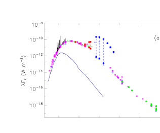
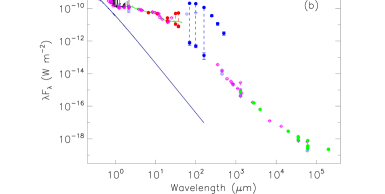
Figure 15: (a) Observed and (b) dereddened SED of MWC 297. Red points are the values derived from SOFIA/FORCAST, while blue points are from Herschel/PACS and SPIRE and green points are from newly measured submm/radio observations. Pink diamonds are values taken from the literature. Blue diamonds are literature values that were not considered in the fit or were combined to generate values shown in pink. Vertical dashed lines connect values for the core and the extended region. Solid black line is the IRTF/SpeX spectrum and solid green line is the ISO spectrum. Solid dark blue line is a Kurucz model for a B1.5 V star, reddened by $A_{V}=8.1$ mag in (a).

Both Manoj et al. (2007) and Alonso-Albi et al. (2009) found that the SED of MWC 297 was rather flat at mm-wavelengths, which they attributed to a population of large grains. However, as pointed out by Sandell, Weintraub & Hamidouche (2011) these authors severely underestimated the free-free emission, which completely dominates the flux densities at millimeter wavelengths. Using all reliable VLA and 3 mm data, Sandell, Weintraub & Hamidouche (2011) found that MWC 297 has a spectral index $\alpha\sim 1.03$. We show a fit to the VLA and BIMA data described in this paper in Figure 16, which is very similar to that shown by Sandell, Weintraub & Hamidouche (2011). The similar fit is also shown by Rumble et al. (2015), who added their SCUBA-2 submillimeter flux densities to their plot. Figure 16 also demonstrates that there is clearly excess flux due to warm dust at 100 $\mu$m and 160 $\mu$m. There appears to be an excess at 450 $\mu$m as well, suggesting that the wind becomes optically thin somewhere between 850 and 450 $\mu$m. With an estimate of the spectral index of the ionized jet in hand, we can estimate the mass loss rate of ionized gas using the ionized jet model developed by Reynolds (1986). (See also eq. 3 in Beltrán et al., 2001.) The jet model requires estimates of the electron temperature, the velocity of the stellar wind, the jet opening angle, and inclination and the turnover frequency where the jet becomes optically thin. We assumed T${}_{e}=10^{4}$ K, consistent with our adopted value for the SpeX analysis, and a wind velocity of $50$ km s^-1, as found from our best fit model of the SpeX spectrum. The jet inclination is 125^∘, as determined from our geometrical modeling of the outflow and the assumption that the disk where the jet originates is perpendicular to the outflow (i.e., the disk inclination is the same as that of the outflow structure). Based on the high angular resolution 6 cm MERLIN image we estimate opening angle of the jet where it is launched to be $\sim 32$^∘. If we assume a turn over frequency (the frequency at which the free-free emission becomes optically thin) of $\sim 400$ GHz 16, the jet model gives a mass loss rate of the ionized gas, $\dot{M}=3.2\times 10^{-7}M_{\odot}~{}\mathrm{yr}^{-1}$, which is within a factor of two of the value derived from modeling the SpeX spectrum. The radius at which the ionized flow in the jet originates is found to be $\sim 19$ au. If a wind velocity of 75 km s^-1is adopted instead, then the predicted mass loss rate is $\dot{M}=4.8\times 10^{-7}M_{\odot}~{}\mathrm{yr}^{-1}$, in reasonable agreement with the value derived from our SpeX analysis.

Figure 16: Least squares fit to the radio and 3 mm flux densities of MWC 297, which yields a spectral index $\alpha\sim$ 1.03. Data points plotted with circles were omitted from the fit. The 850 $\mu$m and 450 $\mu$m flux densities are from Sandell, Weintraub & Hamidouche (2011), while the 160 $\mu$m and 100 $\mu$m PACS data are from this paper. The dot-dash line shows an extension of the fit to shorter wavelengths. There is a clear excess of flux (above the extension to the fit) at 100 $\mu$m and 160 $\mu$m, continuing down to about 450 $\mu$m. The turnover frequency appears to be between 850 and 450 $\mu$m. The dashed line shows the case when the wind becomes optically thin at 400 GHz (750 $\mu$m). Values above the dashed line are due to emission from warm dust.

3.5 The Northeastern Core

The strongest source detected at sub-mm and far infrared wavelengths is a relatively compact core, $\sim$ 20^′′  to the Northeast of MWC 297, which we refer to as the NE Core, see Table 4 and Figure 5. Rumble et al. (2015) labeled it SMM 4 and it is core #68 in Könyves et al. (2015). Rumble et al. (2015) derive a temperature of 46 $\pm$ 2 K and a mass of 2.54 $\pm$ 0.14  M_⊙ (corrected to 418 pc), and argue that it must be heated externally by MWC 297. Könyves et al. (2015) derive a much lower temperature, 23.3 $\pm$ 0.2 K and a mass of 1.6 $\pm$ 0.1  M_⊙, and classify the core as being protostellar, even though there is no embedded source in the core. We derive a smaller core size ($D\sim$ 13 – 14^′′} than both Könyves et al. (2015) and Rumble et al. (2015) by careful background subtraction and hence we derive lower flux densities. A gray body least squares fit gives a temperature of 32 $\pm$ 1 K and a mass of 0.3 $\pm$ 0.05  M_⊙. The temperature we derive is in reasonable agreement with Könyves et al. (2015), considering that their automatic fitting routine almost certainly includes emission from the surrounding cloud.

4 Discussion

4.1 The rotation velocity and nature of the hot star in MWC297

If the spectral type from Drew et al. (1997) and the reddening estimate derived from our spectra and wind models are correct, then the SED we have generated shows that the continuum flux throughout the infrared and even down into the optical wavelength range is predominantly due to dust and bound-free and possibly free-free continuum emission (Fig. 15). If the reddening is $A_{V}\sim 7$ mag, somewhat lower than what we have derived ($A_{V}=8.1$ mag) but still within our uncertainties, then a Kurucz model for a B1.5 V star would match the optical fluxes. However, dust, bound-free, and free-free continuum emission, perhaps due to shocks as a result of the accretion process, generate excess flux at wavelengths at least as short as $\sim 0.8\mu$m and longwards. This is confirmed by our SpeX spectrum, which exhibits strong emission lines and continuum emission, with continuum discontinuities in emission for all three H series we detected, and no discernible sign of stellar absorption lines. It is also consistent with the fractional dust contribution to the $H$ band flux of more than 90% derived by Lazareff et al. (2017), although it is not clear that the dominant source of the excess emission is dust rather than bound-free or free-free emission (see Kluska et al., 2020). This implies that attempts to derive the stellar parameters by fitting reddened stellar models directly to observed continuum fluxes beyond $\sim 0.8\mu$m, and probably at shorter wavelengths as well, without attempting to account for the excess flux, may lead to incorrect results. This may explain why some values for the stellar luminosity, radius, and mass for MWC 297 given in the literature are so much larger than that expected for a B 1.5V star (see e. g. Vioque et al., 2018; Ubeira-Gabellini et al., 2020). Adopting the smaller reddening value leads to a substantially smaller estimate of the total luminosity and therefore a larger discrepancy between the estimated value and that expected for a B1.5V star. Adopting a stellar radius larger than $10R_{\odot}$ to match the optical SED is inconsistent with both the parameters for a B1.5V star and the flux levels at the blue end of our SpeX spectrum.

Using our value of the inclination of the conical dust structure, assuming that the inclination of the central star is the same as that of the outflow, and adopting the stellar rotation rate of $v\sin i=350$ km s^-1 found by Drew et al. (1997) (under the assumption that the broad features detected in the optical spectra are in fact rotationally broadened stellar photospheric lines), we find that the true rotational velocity of the star is very high ($\sim 430$ km s^-1) and only slightly below the critical velocity for a 10 $M_{\odot}$ star with $R\sim 6R_{\odot}$ ($v_{crit}=(2GM_{\ast}/3R_{\ast})^{0.5}\sim 460$ km s^-1; Maeder & Meynet 2000); the ratio of the rotational velocity to the critical velocity is $\sim 0.9$. Furthermore, this value of the true rotational velocity would be well in excess of the critical velocity for a 10 $M_{\odot}$ star with any stellar radius $\geq 7R_{\odot}$. Such a high rotation rate would naturally result in an enhancement of the mass loss at the equator. (See Fig 2 in Maeder & Meynet 2010 for a depiction of the mass loss distribution for a star with properties very similar to those of MWC 297.) Therefore, even though MWC 297 appears to be still accreting, it could well be, simultaneously, in the throes of disruption due to its extreme rotational velocity. Acke et al. (2008) also suggested that the mass loss in MWC 297 may be due to its high rotational velocity and speculated that it may eventually evolve into a classical Be star.

In this regard it is interesting to note the striking differences between the optical spectrum of MWC 297 obtained by Drew et al. (1997) and Fairlamb et al. (2015), obtained in 1994 and 2009, respectively, and that of Andrillat & Jascheck (1998) obtained in 1997. The optical spectra obtained by Drew et al. (1997) and Fairlamb et al. (2015) are very similar, exhibiting strong Balmer emission lines sitting within deep absorption features. Photospheric absorption features from C III, N III, and O II, which Drew et al. (1997) used to determine both the spectral type and the rotational velocity, are present in the Fairlamb et al. (2015) spectra. On the other hand, no photospheric H absorption features can be discerned in the optical spectrum shown by Andrillat & Jascheck (1998), which exhibits a multitude of weak emission lines in the $0.44-0.48\mu$m wavelength region, none of which can be seen in the spectrum presented by Drew et al. (1997). The equivalent widths of the H $\alpha$ and H $\beta$ lines in the spectra from Drew et al. (1997) are a factor of $\sim 2$ larger than those reported by Andrillat & Jascheck (1998). Similarly, the equivalent widths of the H and O I lines given by Fairlamb et al. (2015) are substantially and systematically larger than those listed by Andrillat & Jascheck (1998). However, the equivalent width of the H $\alpha$ line reported by Acke et al. (2005) in data obtained in 2002 was very similar to that measured by Andrillat & Jascheck (1998). We also note that Acke et al. (2005) reported a change in the equivalent width of the [O I] 0.63 $\mu$m line of 25% over a 3 month time period.

We have also retrieved the flux-calibrated X-shooter NIR spectrum obtained by Fairlamb et al. (2015) from the archives and compared it with our SpeX spectrum. The X-shooter spectrum was obtained two years after our SpeX observations. This comparison reveals differences in the strength of both the continuum and the emission lines. The continuum in the $J$ and $H$ bands is a factor of $\sim 2$ stronger in the SpeX data compared to that in the X-shooter spectrum. Similarly, the Pa $\beta$ line flux is nearly a factor of 2 larger in our SpeX spectrum, while the Br $\gamma$ line, which is quite strong in our SpeX data, is nearly indistinguishable above the noise in the spectrum obtained by Fairlamb et al. (2015). Fairlamb et al. (2015) give only an upper limit for flux of the Br $\gamma$ line that is a factor of 12 lower than the flux we directly measure in our SpeX spectrum. The O I 0.8446 $\mu$m line is somewhat stronger in the X-shooter spectrum than in our SpeX data. Fairlamb et al. (2015) also report fluxes for the Ca II triplet at 0.85 $\mu$m that are significantly larger than the fluxes we measure in the nearby upper Paschen series; we see no evidence of Ca II emission in our SpeX spectrum. (Andrillat & Jascheck 1998 also did not detect the Ca II lines.) Given the differences in H line strengths, it is not surprising that the mass accretion rate we derive from the strongest emission line strengths in the SpeX spectrum is considerably larger than that reported by Fairlamb et al. (2015), even after accounting for the different distances used in the calculation. We also note that although the He I $1.083\mu$m line in our spectrum exhibits a P Cygni profile (with two blue absorption features), indicating formation in an outflowing wind, we see no sign of absorption at He I 2.058 $\mu$m, as reported by Murdoch & Drew (1994) (although the absorption could possibly be masked by residuals from the telluric correction in our spectrum).

The optical photometry of MWC 297, as well as the fluxes of the strongest H emission lines reported in the literature, combined with the results of this comparison indicate considerable, rapid variability in both the continuum and the emission line strengths of the source. It is possible that this irregular ’flickering’ of the source strength in MWC 297 is due to the unstable nature of the central star as a result of its high rotational velocity, extremely close to the break-up velocity. Examination of the Herschel PACS image 4, as well as the WISE, Spitzer, and 2MASS images of MWC 297 reveal numerous arcs of emission at a range of radii up to $\sim 1.5$ pc from the central star in MWC 297 (see e. g. Wang & Looney, 2007). The appearance of these structures, combined with the variability of the accretion and mass-loss rates (as evidenced by the variable H emission line strengths), suggests that MWC 297 has experienced multiple mass ejection events since its formation. It is tempting to speculate that these ejection events are due to the high rotational velocity of the star, perhaps combined with the orbital effects of the close companions discovered by Ubeira-Gabellini et al. (2020) and Sallum et al. (2021), which may be modulating the accretion rate from the central disk.

4.2 The accretion disk in MWC 297

Observations of double-peaked CO lines in NIR spectra (Banzatti et al., 2022; Sandell & Vacca, 2022) clearly indicate that an accretion disk is present in MWC297. However, the stellar rotational velocity, corrected for the inclination, indicates that the disk co-rotation radius, $R_{cor}=(GM_{\ast}R_{\ast}/v_{\ast}^{2})^{1/3}$, must be $\sim 7R_{\odot}$. Since the disk truncation radius must be smaller than the co-rotation radius, the accretion disk must extend down to nearly the stellar surface in MWC 297. Acke et al. (2008) and Kluska et al. (2020) reached a similar conclusion from modeling their interferometric data on MWC297, which failed to reveal an inner gap or cavity between the disk and the star. This result strengthens the claim that the model of magnetospheric accretion, widely accepted for lower mass Classical T Tauri stars, is probably not applicable to Herbig Be stars (see e.g. Mottram et al., 2007; Mendigutia et al., 2011; Wichittanakom et al., 2020). The boundary layer theory of accretion, proposed by Lynden-Bell & Pringle (1974), accompanied by a radiation-driven wind from either the star itself or the disk, as proposed by Drew, Proga, & Stone (1998), appears to be the more appropriate model for high luminosity objects like MWC 297.

It is unclear why the orientation of the system, derived directly from our MIR images, is so different from the values derived from interferometric analyses. While it is beyond the scope of this paper to investigate the reasons for this discrepancy, we can speculate about possible causes. It is possible that the inner source has rotated and the larger scale orientation that we observe in our FORCAST images does not reflect that of the inner disk (i.e., the inner disk is tilted.) However, given the young age of the system ($\sim 0.1$ Myr) and the magnitude of the inclination discrepancy ($>15$ ^∘), it is not clear how such a large misalignment of the disk and the larger-scale structure would have occurred in such a short time. The examples of systems with misaligned inner disks among HAeBe stars are generally fairly old (e.g., AB Aur and HD 100546, which have ages of several million years; van den Ancker et al. 1998; DeWarf et al. 2003). Furthermore, the radio data, which traces the outflow from its origin in the inner disk and therefore presumably does reflect the orientation of the inner disk, seems to be well aligned with the structure we see in the FORCAST images. In addition, Sallum et al. (2021) have derived disk inclinations similar to those we have found from our direct MIR observations from analysis of their interferometric data when they include an outflow along with an inclined disk in their models. They claim that the disk plus outflow model provides the best representation of the observed brightness distribution in their data. Their modeling also yields a position angle of the outflow that is similar to ours.

A possibly more likely explanation for the discrepancy in the inclination values is that the interferometric analyses are in error simply because the assumptions involved in the modeling the data are incorrect or incomplete. Malbet et al. (2007) modeled AMBER/VLTI observations of MWC 297 in the Br $\gamma$ line using a combination of an optically thick gas disk and an optically thin wind. However, our models suggest that the latter assumption is invalid in MWC 297, for which all of the NIR lines appear to be optically thick, and Br $\gamma$ extremely so. Interferometric studies often find that the Br $\gamma$ emitting region in MWC 297 is more extended than the region that generates the continuum emission Malbet et al. (e.g. 2007); Kraus et al. (e.g. 2008); Hone et al. (e.g. 2017). Most models used to interpret these results assume that the continuum emission is due to dust in the accretion disk close to the star (e.g. Millan-Gabet at al., 2001; Eisner et al., 2004; Acke et al., 2008; Kraus et al., 2008). These models usually encounter difficulties as they yield locations for the emission regions that are so close to the star that the temperature of the dust which is supposed to be responsible for the emission is beyond the sublimation limit. Our SpeX data, in which strong continuum jumps due to bound-free emission can be clearly seen, suggest that the assumption that emission from dust is the predominant component of the NIR flux may be incorrect. Instead, an optically thick gaseous region close to the star may be responsible for this flux via bound-free or free-free emission (see also Acke et al., 2008; Kluska et al., 2020). Muzerolle et al. (2004) has shown that emission from an optically thick gaseous inner disk region may be a substantial contributor to the NIR flux in sources with accretion rates as high as that we estimate for MWC 297. Our results, combined with those of Sallum et al. (2021), suggest that interpretation of interferometric data needs to be approached with some caution, as models which do not include important physical aspects of the system may lead to erroneous results.

5 Summary and Conclusions

Our SOFIA/FORCAST images at 20-40 $\mu$m provide a unique and direct view of the dust surrounding the massive Herbig Be star MWC 297. We interpret the extended MIR emission seen in the FORCAST images as arising from warm ($T_{dust}\sim 67$ K), optically thin dust entrained at the edges of the bi-polar outflow that is seen in our VLA and BIMA radio data. The structure seen in the MIR images reflects the conical shape expected from such a scenario. The southern arc is in the foreground, tipped toward the observer, while the northern annulus is tipped away. We constructed a simple geometrical model of the system and generated simulated MIR images to constrain the physical parameters. We find the inclination of the system to be $i\sim 55$ ^∘, which directly contradicts the low inclination values derived from the analysis of the previous interferometric observations. Nevertheless, our derived inclination value agrees with the approximately N-S extension of the ionized flow seen in the radio maps of Sandell, Weintraub & Hamidouche (2011) as well as the recent results of the interferometric images and analysis by Sallum et al. (2021). The inclination value implies that the central star in MWC 297 must be rotating close to its break-up velocity. Furthermore, the inclination allows us to estimate the truncation radius of the accretion disk, which must be close to the stellar surface. This result provides further evidence that the magnetospheric accretion model is not applicable to high mass Herbig Be stars.

Our NIR spectrum of MWC 297 obtained with SpeX reveals a host of strong emission lines, most from the Paschen, Brackett, and Pfund series of H, and continuum emission that rises to longer wavelengths. Continuum jumps from the H series are seen in emission. Although the He I $1.083\mu$m line exhibits a P Cygni profile, no other absorption features are seen in this spectrum. We modeled the H line emission with a wind model and find that all of the lines are optically thick. The analysis yields a mass-loss rate for the system of $\sim 6\times 10^{-7}M_{\odot}{\rm yr}^{-1}$ and an extinction of $A_{V}=8.1$ mag. The ionization rate needed to generate these lines is far above that expected from a B1.5V star atmosphere, and therefore most of the ionizing flux must arise from the accretion process.

We compiled data from the literature and combined it with our FORCAST, VLA, and BIMA measurements and archival Herschel data to generate the SED of MWC 297 from $0.35~{}\mu$m to $6$ cm. Integrating under the SED, we calculate a total luminosity of MWC 297 of $\sim 6900L_{\odot}$, somewhat less than that expected for a B1.5V star, although we are certainly missing flux from unobserved wavelength regions. After accounting for flux between 0.25 and 0.35 $\mu$m, we estimate a bolometric luminosity of MWC 297 of $\sim 7900L_{\odot}$, with an upper limit of $\sim 10200~{}L_{\odot}$ The SED analysis reinforces the suggestion of Acke et al. (2008) that the extinction we measure from the H lines with the wind model is due to foreground dust, distant from the star, and not the dust we detect in the immediate vicinity.

Finally, we speculate that the high rotational velocity ($\sim 430$ km s^-1, or $\sim 90$% of the break-up velocity) of the central star in MWC 297, perhaps combined with the orbital effects of the two possible nearby low-mass companions recently detected via interferometry, may be responsible for the rapid fluctuations in the mass accretion and mass-loss rates from the central disk. These fluctuations would then produce the variations observed in the continuum and emission line strengths.

Table 1: MWC 297 line fluxes measured with IRTF/SpeX

Obs. Wavelength	Obs. Flux	Uncertainty	ID
($\mu$m)	($10^{-16}$ W m-2)
0.832663	2.53	0.66	Pa 25
0.833688	5.48	0.91	Pa 24
0.834848	5.97	0.62	Pa 23
0.836198	8.37	0.48	Pa 22
0.837740	10.30	0.47	Pa 21
0.839541	11.87	0.45	Pa 20
0.841625	15.83	0.48	Pa 19
0.844929	261.57	0.64	Pa 18 + O I
0.847015	21.92	0.46	Pa 17
0.850542	24.34	0.43	Pa 16
0.854833	27.52	0.41	Pa 15
0.860108	34.89	0.41	Pa 14
0.863217	6.34	0.33	N I
0.866803	37.41	0.38	Pa 13
0.868566	18.80	0.41	N I
0.875349	42.55	0.36	Pa 12
0.886589	52.12	0.35	Pa 11
0.901800	61.24	0.39	Pa 10
0.906406	5.18	0.31
0.909760	6.03	0.36	C I
0.923224	86.59	0.44	Pa 9
0.924724	10.70	0.39	Mg II
0.926710	10.85	0.44	O I
0.954920	131.62	0.53	Pa $\epsilon$
1.000116	13.00	0.22
1.005296	233.13	0.45	Pa $\delta$
1.011420	14.02	0.26
1.017763	1.80	0.21
1.029057	2.14	0.21	[S II]
1.032398	2.68	0.16	[S II]
1.043853	1.19	0.24
1.046021	2.37	0.21
1.050532	10.88	0.21
1.053146	19.74	0.63
1.072321	54.94	0.81
1.083737	23.18	0.25	He I
1.086643	11.22	0.23
1.091859	12.89	0.27
1.094196	528.52	0.90	Pa $\gamma$
1.112957	10.71	0.33
1.116940	12.51	0.83
1.129121	446.46	0.82	O I
1.175703	27.07	0.23	C I
1.189867	4.80	0.18
1.200254	1.71	0.18
1.213768	2.38	0.21
1.219186	4.12	0.20
1.220817	2.85	0.21
1.233349	4.31	0.20
1.238663	6.81	0.20
1.240800	2.10	0.22
1.246987	31.59	0.29
1.257211	12.21	0.42
1.261574	7.45	0.38
1.282257	1588.64	1.78	Pa $\beta$
1.316919	89.94	0.36	O I
1.343495	12.81	0.37
1.454872	16.53	0.37
1.482794	23.14	1.66
1.485319	5.42	0.31	Br 30
1.487256	10.83	0.41	Br 29
1.489312	12.97	0.32	Br 28
1.491721	14.37	0.31	Br 27
1.494332	18.95	0.32	Br 26
1.497276	25.21	0.33	Br 25
1.500623	27.39	0.33	Br 24
1.504437	36.56	0.37	Br 23
1.508821	38.67	0.36	Br 22
1.513864	47.09	0.36	Br 21
1.519726	54.77	0.36	Br 20
1.526598	58.65	0.36	Br 19
1.534724	66.29	0.38	Br 18
1.544442	78.16	0.39	Br 17
1.556195	88.31	0.41	Br 16
1.558674	11.62	0.33
1.570623	98.93	0.44	Br 15
1.588622	123.30	0.49	Br 14
1.611500	150.41	0.56	Br 13
1.641303	157.17	0.61	Br 12
1.681246	164.14	0.71	Br 11
1.682854	81.20	1.90
1.703959	11.72	1.35
1.736831	187.78	0.97	Br 10
1.945248	380.34	1.78	Br 8
2.059333	22.94	1.29	He I
2.166293	512.79	1.42	Br $\gamma$
2.329991	8.05	1.05	Pf 34
2.333117	10.30	1.28	Pf 33
2.336679	13.03	1.44	Pf 32
2.340345	16.19	1.46	Pf 31
2.344606	10.74	1.03	Pf 30
2.349666	17.21	1.46	Pf 29
2.354513	25.41	1.52	Pf 28
2.360591	20.14	1.22	Pf 27
2.367197	28.05	1.56	Pf 26
2.374560	27.92	1.64	Pf 25
2.383186	28.52	1.41	Pf 24
2.392506	30.58	1.32	Pf 23
2.403738	31.52	1.37	Pf 22
2.416510	42.94	1.69	Pf 21

References

- Acke et al. (2008) Acke, B., et al. 2008, A&A, 485, 209
- Acke et al. (2005) Acke, B., van den Ancker, M. E., & Dullemond, C. P. 2005, A&A, 436, 209
- Allen & Swings (1972) Allen, D. A., & Swings, J. P. 1972, A&A, 47, 293
- Alonso-Albi et al. (2009) Alonso-Albi, T., Fuente, A., Bachiller, R., et al. 2009, A&A, 497, 117
- André et al. (2010) André, Ph., MenÕshchikov, A., Bontemps, S., et al. 2010, A&A, 518, L102
- Andrillat & Jascheck (1998) Andrillat, Y., & Jaschek, C. 1998, A&AS, 131, 479
- Banzatti et al. (2022) Banzatti, A., Abernathy, K. M., Brittain, S., Bosman, A. D., Pontoppidan, K. M., Boogert, A., Jensen, S., Carr, J., Najita, J., Grant, S., Sigler, R. M., Sanchez, M. A., Kern, J., & Rayner, J. T. 2022, arXiv:2202.03438v1
- Beltrán et al. (2001) Beltrán, M. T., Estalella, R., Anglada, G., et al. 2001, AJ, 121, 1556
- Benedettini et al. (1998) Benedettini, M., Nisini, B., Giannini, T., Lorenzetti, D., Tommasi, E., Saraceno, P., & Smith, H. A. 1998, A&A, 339, 159
- Benedettini et al. (2001) Benedettini, M., Pezzuto, S., Giannini, T., Lorenzetti, D., & Nisini, B. 2001, A&A, 379, 557
- Berrilli et al. (1992) Berrilli, F., Corciulo, G., Ingrosso, G., Lorenzetti, D., Nisini, B., & Strafella, F. 1992, ApJ, 398, 254
- Bohm-Vitense (1981) Böhm-Vitense, E. 1981, ARAA, 19, 295
- Bontemps et al. (2010) Bontemps, S., André, Ph., Könyves, V., et al. 2010, A&A, 518, L85
- Cantó et al. (1981) Cantó, J., Rodríguez, L. F., Barral, J. F., & Carral, P. 1981, ApJ, 244, 102
- Cardelli, Clayton & Mathis (1989) Cardelli, J. A., Clayton, G. C., & Mathis, J. S. 1989, ApJ, 345, 245
- Castelli & Kurucz (1994) Castelli, F. & Kurucz, R. L. 1994, A&A, 281, 817
- Castor (1970) Castor, J. I. 1970, MNRAS, 149, 111
- Chambers et al. (2016) Chambers, K. C. et al. 2016, arXiv:1612.05560
- Clarke et al. (2021) Clarke, M., Vacca, W., Chambers, E., & Radomski, J. 2021, FORCAST Redux Users Manual, SCI-IS-HBK-OP10-2003
- Cohen et al. (2001) Cohen, M., Walker, R. G., Jayaraman, S., Barker, E., & Price, S. D. 2001, AJ, 121, 1180
- Cohen et al. (2003) Cohen, M., Wheaton, Wm. A., & Megeath, S. T. 2003, AJ, 126, 1090
- Cushing, Vacca & Rayner (2004) Cushing, M. C., Vacca, W. D., & Rayner, J. T. 2004, PASP, 116, 362
- DeWarf et al. (2003) DeWarf, L. E., Sepinsky, J. F., Guinan, E. F., Ribas, I., & Nadalin, I. 2003, ApJ, 590, 357
- DeWinter et al. (2001) de Winter, D., van den Ancker, M. E., Maira, A., Thé, P. S., Tjin A Djie, H. R. E., Redondo, I., Eiroa, C., & Molster, F. J. 2001, A&A, 609
- Di Francesco et al. (1998) Di Francesco, J., Evans II, N. J., Harvey, P. M., Mundy, L. G., & Butner, H. M. 1998, ApJ, 509, 324
- Drew et al. (1997) Drew, J. E., Busfield, G., Hoare, M. G., et al. 1997, MNRAS, 286, 538
- Drew, Proga, & Stone (1998) Drew, J. E., Proga, D., & Stone, J. M. 1998, MNRAS, 296, L6
- Eisner et al. (2004) Eisner, J. A., Lane, B. F., Hillenbrand, L. A., Akeson, R. L., & Sargent, A. I. 2004, ApJ, 613, 1049
- Eisner et al. (2015) Eisner, J. A., Rieke, G. H., Rieke, M. J., Flaherty, K. M., Stone, J. M., Arnold, T. J., Cortes, S. R., Cox, E., Hawkins, C., Cole, A., Zajac, S., & Rudolph, A. L. 2015, MNRAS, 447, 202
- Fairlamb et al. (2015) Fairlamb, J. A., Oudmaijer, R. D., Mendigutía, I., et al. 2015, MNRAS, 453, 976
- Fairlamb et al. (2015) Fairlamb, J. A., Oudmaijer, R. D., Mendigutía, I., et al. 2015, MNRAS, 453, 976
- Felli & Panagia (1981) Felli, M. & Panagia, N. 1981, A&A, 102, 424
- Finkenzeller & Mundt (1984) Finkenzeller, U., & Mundt, R. 1984, A&AS, 55, 109
- Fouque et al. (2000) Fouqué, P. et al. 2000, \aas, 141, 313
- Gibb & Hoare (2007) Gibb, A. G., & Hoare, M. G. 2007, MNRAS, 380, 246
- Groenewegen & Lamers (1989) Groenewegen, M A. T. & Lamers, H. J. G. L. M. L. 1989, A&AS. 79, 359
- Gutermuth et al. (2009) Gutermuth, R. A., Megeath, S. T., Myers, C. P., et al. 2009, ApJS, 184, 18
- Guzman-Diaz et al. (2021) Guzmán-Díaz, J., Mendigutía, I., Montesinos, B., Oudmaijer, R. D., Vioque, M., Rodrigo, C., Solano, E., Meeus, G., & Marcos-Arenal, P. 2021, A&A, 650, A182
- Habart et al. (2003) Habart, E., Testi, L., Natta, A., & Vanzi, L. 2003, A&A, 400, 575
- Henden et al. (2015) Henden, A. A., Stephen, L., Dirk, T., & Welch, D. L. 2015, AAS225, 336.16
- Henning et al. (1998) Henning, Th., Burkert, A., Launhardt, R., Leinert, Ch., & Stecklum, B. 1998, A&A, 336, 565
- Herbig (1960) Herbig, G. H. 1960, ApJS, 4, 337
- Herter et al. (2013) Herter, T. L., Vacca. W. D., Adams, J. D., et al. 2013 PASP, 125, 1393
- Herter et al. (2012) Herter, T. L., Adams, J. D., De Buizer, J. M., et al. 2012, ApJ, 749, L18
- Hillenbrand et al. (1992) Hillenbrand, L. A., Strom, S. E., Vrba, F. J., & Keene, J. 1992, ApJ, 397, 613
- Hone et al. (2017) Hone, E., Kraus, S., Kreplin, A., Hofmann, K.-H., Weigelt, G., Harries, T., & Kluska, J. 2017, A&A, 607, A17
- Jinliang et al. (1997) Jinliang, H., Dongrong, J., & Chengqi, F. 1997, A&A, 327, 725
- Kimeswenger et al. (2004) Kimeswenger, S. et al. 2004, A&A, 413, 1037
- Kluska et al. (2020) Kluska, J., Berger, J.-P., Malbet, F., et al. 2020, A&A, 636, A116
- Könyves et al. (2015) Könyves, V., André, Ph., Men’shchikov, A., et al. 2015, A&A, 584, A91
- Könyves et al. (2010) Könyves, V., André, Ph., Men’shchikov, A., et al. 2010, A&A, 518, L106
- Kraus et al. (2008) Kraus, S. et al. 2008, A&A, 489, 1157
- Kurucz (1992) Kurucz, R. L. 1992, in IAU Symp. 149, The Stellar Populations of Galaxies, ed. B. Barbuy & A. Renzini (Dordrecht: Kluwer), 225
- Lamers & Pauldrach (1991) Lamers, H. J. G. L. M. & Pauldrach, A. W. A. 1991, A&A, 244, L5
- Lanz & Hubeny (2007) Lanz, T. & Hubeny, I. 2007, ApJS, 169, 83
- Lazareff et al. (2017) Lazareff, B., Berger, J.-P., Kluska, J., et al. 2017, A&A, 599, A85
- Lupton et al. (1999) Lupton, R. H., Gunn, J. E., &Szalay, A. S. 1999, AJ, 118, 1406
- Lynden-Bell & Pringle (1974) Lynden-Bell, D. & Pringle, J. E. 1974, MNRAS, 168, 603
- Maeder & Meynet (2000) Maeder, A. & Meynet, G. 2000, A&A, 361, 159
- Maeder & Meynet (2010) Maeder, A. & Meynet, G. 2010, New Astronomy Reviews, 54, 32
- Malbet et al. (2007) Malbet, F. et al. 2007, A&A, 464, 43
- Mann & von Braun (2015) Mann, A. W. & von Braun, K. 2015, PASP, 127, 102
- Manoj et al. (2007) Manoj, P., Ho, P. T. P., Ohashi, N., et al. 2007, ApJ, L187
- Mannings (1994) Mannings, V. 1994, MNRAS, 271, 587
- McClure (2009) McClure, M. 2009, ApJ, 693, L81
- Mendigutia et al. (2011) Mendigutía, I., Calvet, N., Montesinos, B., Mora, A., Muzerolle, J., Eiroa, C., Oudmaijer, R. D., & Merín, B. 2011, A&A, A99
- Millan-Gabet at al. (2001) Millan-Gabet, R., Schloerb, F. P., & Traub, W. A. 2001, ApJ, 546, 358
- Mottram et al. (2007) Mottram, J. C., Vink, J. S., Oudmaijer, R. D., & Patel, M. 2007, MNRAS, 377m 1363
- Murdoch & Drew (1994) Murdoch, K. A. & Drew, J. E. 1994, in ASP Conf. Ser. 62, The Nature and Evolutionary Status of Herbig Ae/Be Stars, 377
- Muzerolle et al. (2004) Muzerolle, J., D’Alessio, P., Calvet, N., & Hartmann, L. 2004, ApJ, 617, 406
- Nisini et al. (2004) Nisini, B. Antoniucci, S., & Giannini, T. 2004, A&A, 421, 187
- Nisini et al. (1995) Nisini, B. Milillo, A., Saraceno, P., & Vitali, F. 1995, A&AS, 302, 169
- Ortiz-León et al. (2017) Ortiz-León, G. N., Dzib, S. A., Kounkel, M. A., et al. 2017, ApJ, 834, 143
- Oudmaijer & Drew (1999) Oudmaijer, R. D. & Drew, J. E. 1999, MNRAS, 305, 166
- Peraiah (2002) Peraiah, A. 2002, An Introduction to Radiative Transfer, Cambridge: Cambridge University Press
- Price et al. (2001) Price, S. D., Egan, M. P., Carey, S. J., Mizuno, D. R., & Kuchar, T. A. 2001, AJ, 121, 2819
- Puls et al. (1996) Puls, J., Kudritzki, R.-P. Herrero, A., Pauldrach, A. W. A., Hase, E. M., Lennon, D. J., Gabler, R., Voels, S. A., Vilchez, J. M., Wachter, S., & Feldmeier, A. 1996, A&A, 305, 171
- Raga et al. (1993) Raga, A. C., Cantó, J., Calvet, N., Rodríguez, L. F., & Torrelles, J. M. 1993, A&A, 276, 539
- Rayner et al. (2003) Rayner, J. T., Toomey, D. W., Onaka, P. M., et al.. 2003, PASP, 115, 362
- Rayner, Cushing & Vacca (2009) Rayner, J. T., Cushing, M. C., & Vacca, W. D. 2009, ApJS, 185, 289
- Reynolds (1986) Reynolds, S. P. 1986, ApJ, 304, 713
- Richmond et al. (2000) Richmond, M. W., Droege, T. F., Gombert, G., Gutzwiller, M., Henden, A. A., Albertson, C., Beser, N., Molhant, N., & Johnson, H. 2000, PASP, 112, 397
- Ridge et al. (2003) Ridge, N. A., Wilson, T. L., Megeath, S. T., et al. 2003, AJ, 126, 286
- Riello et al. (2021) Riello, M. et al. 2021, A&AS, 649, A3
- Rumble et al. (2015) Rumble, D., Hatchell, J., Gutermuth, R. A., et al. 2015, MNRAS, 488, 1551
- Sallum et al. (2021) Sallum, S., Eisner, J. A., Stone, J. M., et al. 2021, ApJ, 161, 28
- Sandell, Weintraub & Hamidouche (2011) Sandell, G., Weintraub, D. A., & Hamidouche, M. 2011, ApJ, 727, 26
- Sandell et al. (2009) Sandell, G., Goss, W. M., Wright, M., & Corder, S. 2009, ApJ, 699, L31
- Sandell & Vacca (2022) Sandell, G. & Vacca, W. D. 2022, submitted
- Sault, Teuben & Wright (1995) Sault, R. J., Teuben, P. J., & Wright, M. C. H. 1995, in ASP Conf. Ser. 77, Astronomical Data Analysis Software and Systems IV, ed. R. A. Shaw, H. E. Payne, & J. J. E. Hayes (San Francisco, CA: ASP), 433
- SchmidtKaler (1982) Schmidt-Kaler, T. 1982, in Landolt-Börnstein, New Series, Group VI, Vol. 2, ed. K. Schaifers & H. H. Voigt(Berlin: Springer-Verlag), 1
- Shuping et al. (2012) Shuping, R. Y., Morris, M., R., Herter, T. L., Adams, J. D., Gull, G. E., Schoenwald, J., Henderson, C. P., Becklin, E. E., De Buizer, J. M., Vacca, W. D., Zinnecker, H., & Megeath, S. T. 2012, ApJ, 749, L22
- Simon (1974) Simon, T. 1974, AJ, 79, 1054
- Skinner, Brown, & Stewart (1993) Skinner, S. L., Brown, A., & Stewart, R. T. 1993 ApJS, 87, 217
- Sobolev (1960) Sobolev, V. V. 1960, Moving Atmospheres of Stars, Cambridge: Harvard University Press
- Storey & Hummer (1995) Storey, P. J. & Hummer, D. G. 1995, MNRAS, 272, 41
- Stapper et al. (2022) Stapper, L. M., Hogerheijde, M. R., van Dishoeck, E. F., & Mentel, R.¯2022, A&A, 658, A112
- Thé, de Winter and Pérez (1994) Thé, P. S., de Winter, D., & Pérez, M. R. 1994, A&AS, 104, 315
- Tonry et al. (2012) Tonry, J. L. et al. 2012, ApJ, 750, 99
- Tuthill et al. (2002) Tuthill, P. G., Monnier, J. D., Danchi, W. C., Hale, D. D. S., & Townes, C. H. 2002, ApJ, 577, 826
- Ubeira-Gabellini et al. (2020) Ubeira-Gabellini, M. G., Christiaens, V., Lodato, G., et al. 2020, ApJ, 890, L8
- Vacca, Cushing & Rayner (2003) Vacca, W. D., Cushing, M. C. & Rayner, J. T. 2003, PASP, 115, 389
- van den Ancker et al. (1998) van den Ancker, M. E., de Winter, D., Tjin A Djie, H. R. E. 1998, A&A, 330, 145
- Verhoeff et al. (2012) Verhoeff, A. P., Waters, L. B., F. M., van den Ancker, M. E., et al. 2012, A&A, 538, A101
- Vioque et al. (2018) Vioque, M., Oudmaijer, R. D., Baines, D., et al. 2018, A&A, 620, A128
- Wang & Looney (2007) Wang, S., & Looney, L. W. 2007, ApJ, 659, 1360
- Waters & Waelkens (1998) Waters, L. B. F. M. & Waelkens, C. 1998, ARA&A, 36, 233
- Weigelt et al. (2011) Weigelt, G. et al. 2011, A&A, 527, A103
- Wichittanakom et al. (2020) Wichittanakom, C., Oudmaijer, R. D., Fairlamb, J. R., Mendigutía, I., Vioque, M., & Ababakr, K., M. 2020, MNRAS, 234
- Wolf et al. (2018) Wolf, C. et al. 2018, PASA, 35, 1
- Yuldoshev et al. (2017) Yuldoshev, W. X., Ehgamberdiev, Sh. A., Muminov, M. M., Protsyuk, Yu. I., Relke, H., & Andruk, V. M. 2017, Kinematics and Physics of Celestial Bodies, 33, 250
- Zacharias et al. (2015) Zaharias, N. et al. 2015, AJ, 150, 101
- Zickgraf (2003) Zickgraf, F.-J. 2003, A&A, 408, 257