PL-$k$NN: A Parameterless Nearest Neighbors Classifier

Abstract

Demands for minimum parameter setup in machine learning models are desirable to avoid time-consuming optimization processes. The $k$-Nearest Neighbors is one of the most effective and straightforward models employed in numerous problems. Despite its well-known performance, it requires the value of $k$ for specific data distribution, thus demanding expensive computational efforts. This paper proposes a $k$-Nearest Neighbors classifier that bypasses the need to define the value of $k$. The model computes the $k$ value adaptively considering the data distribution of the training set. We compared the proposed model against the standard $k$-Nearest Neighbors classifier and two parameterless versions from the literature. Experiments over 11 public datasets confirm the robustness of the proposed approach, for the obtained results were similar or even better than its counterpart versions.

I Introduction

Data classification is the most popular approach in machine learning. The paradigm comprises a set of labeled samples used to train a specific model, i.e., to learn intrinsic characteristics from data, for further classification of unlabeled instances. In this context, one can refer to traditional methods such as the Support Vector Machines [1] and Artificial Neural Networks [2], as well as graph-based models, such as the Optimum-Path Forest [3] and the $k$-Nearest Neighbors ($k$-NN) [4]. $k$-NN is a method used for both classification [5] and regression [6] purposes. It obtained notorious popularity in the last three decades due to its competitive results in a wide variety of domains, ranging from medicine [7] to engineering [8], and sentiment analysis [9]. Although efficient and straightforward, $k$-NN is sensitive to the proper selection of the $k$ value, which may denote a stressful task to the user. A similar problem is faced by most machine learning methods and has been commonly overpassed through metaheuristic optimization algorithms [10]. Regarding $k$-NN, Wicaksono and Supianto [11] recently employed such approaches to model the problem of selecting an appropriate $k$. Ling et al. [12] proposed a distance-based strategy to choose the best $k$ by considering a region centered in each instance of the test set. On the other hand, Zhang and Song [13] proposed a neural network-based model to predict the best $k$ by considering a set of features extracted from each sampled dataset. Besides, Singh et al. [14] proposed a parameterless version of the $k$-NN algorithm for regression purposes. Similar work presented by Desai et al. [15] also claims a parameterless version of $k$-NN for regression purposes. However, the model requires four extra hyperparameters. Ayyad et al. [5] proposed a modified version of the $k$-NN classifier for gene expression cancer classification. The proposed model defines a circle with radius $r$ centered at the test sample under prediction, where $r$ is computed by two versions of their Modified $k$-NN (MKNN) model: Smallest MKNN (SMKNN) and Largest MKNN (LMKNN), which measure the minimum and maximum distance between the test sample and each class centroid of the training set, respectively. Although effective in the context of gene data analysis, the method may still suffer from the high amount of neighbors in cases where the class centroids are distant from each other.

This paper proposes the Parameterless $k$-Nearest Neighbors (PL-$k$NN) classifier, a $k$-Nearest Neighbors variant that avoids selecting the proper value of $k$ by introducing a mechanism that automatically chooses the number of neighbors that correctly matches the data distribution. The proposed model is similar to SMKNN presented by Ayyad et al. [5]; however, we suggest the following two improvements:

• To use the median sample instead of the mean sample as the class centroid;

• To use a semicircle whose radius is defined as the distance of the test sample to the nearest class centroid.

Regarding the second contribution, we want to find the training samples assumed to be as close as possible to the nearest centroid of the test sample under prediction. This approach is efficient when there is a mixing of training samples of different classes. In this case, the proposed model defines a semicircle enclosing only the nearest samples close to the cluster assumed as the class of the test instance.

The remainder of the paper is organized as follows: Section II introduces the proposed PL-$k$NN model. Afterward, Sections III and IV present the methodology and the experimental results, respectively. Finally, Section V states conclusions and future work.

II Proposed method

Let ${\cal Y}=\{\omega_{1},\omega_{2},\omega_{3},\dots,\omega_{n}\}$ be the set of classes from the dataset, where $\omega_{i}$ represents the $i^{th}$ class. Also, let ${\cal X}={\{\bm{x}_{1},\bm{x}_{2},\bm{x}_{3},\dots,\bm{x}_{m}\}}$ be the set of samples of the dataset represented by a feature vector denoted as $\bm{x}_{j}\in R^{d}$. In the supervised classification approach, each sample $\bm{x}_{j}$ is assigned to a class $y_{j}\in{\cal Y}$ such that the pair $(\bm{x}_{j},y_{j})$ is used in the subsequent training and testing of the classifier. Formally speaking, this step involves partitioning the samples such that ${\cal X}={\cal X}_{1}\cup{\cal X}_{2}$ and ${\cal X}_{1}\cap{\cal X}_{2}=\emptyset$, where ${\cal X}_{1}$ and ${\cal X}_{2}$ denote the training and testing sets, respectively.

In the proposed method, the training set is split into $n$ clusters that represent each class $y_{i}\in{\cal Y}$. Further, the number of nearest neighbors $k$ connected to a target sample $\bm{x}_{j}$ is adaptively defined according to its distance to all training samples inside the radius of the nearest cluster’s centroid. Let ${\cal C}=\{\bm{c}_{1},\bm{c}_{2},\ldots,\bm{c}_{n}\}$ be the set of centroids such that $c_{i}$ denotes the centroid of the $i^{th}$ cluster, which contains all samples from ${\cal X}_{1}$ that belong to class $\omega_{i}$. The training stage of the proposed model is summarized as follows:

1. Cluster the dataset into $n$ clusters;

2. For each sample $\bm{x}_{i}\in{\cal X}_{1}$, assign it to the $y_{i}^{th}$ cluster;

3. For each $y_{i}^{th}$ cluster, compute its centroid $\bm{c}_{y_{i}}$ as the median sample;

4. Compute the weight of each training sample $\bm{x}_{i}$ regarding its centroid $\bm{c}_{y_{i}}$ using $W(\bm{x}_{i},\bm{c}_{y_{i}})=D_{E}(\bm{x}_{i},\bm{c}_{y_{i}})^{-1}$, where $D_{E}(\bm{x}_{i},\bm{c}_{y_{i}})$ denotes the Euclidean distance between sample $\bm{x}_{i}$ and the centroid $\bm{c}_{y_{i}}$;

5. Repeat steps 2-4 for all samples in ${\cal X}_{1}$.

The training stage is similar to SMKNN, except for the class centroid computation, whose value is computed from the average of each training sample’s features in the SMKNN variant.

The PL-$k$NN training stage consists of finding the cluster centroid and the distance weights of all training samples. The distance is computed between each training sample $\bm{x}_{i}\in{\cal X}_{1}$ and the centroid $\bm{c}_{y_{i}}$ of its cluster. Step 1 is concerned with the splitting of the dataset into $n$ clusters according to the number of classes in ${\cal Y}$. In Step 2, each training sample $\bm{x}_{i}$ is assigned to the cluster of its class $y_{i}$. Step 3 finds the samples assumed to be the center of each cluster by computing its median feature vector. This approach is more effective than using the average due to the following reasons: i) the average is not a valid instance of the cluster, although it is assumed to be located as close as possible to its center, and ii) the average is more sensitive to outliers, and consequently, the resulting value may differ from the data distribution center. In contrast, the median is the sample in the middle of the data distribution, which reduces the effect of instances distant from the dense region of the cluster. Step 4 is defined to assign a weight for all instances inside the cluster. The more distant from the centroid, the smaller the weight of the training sample. Samples distant from the cluster will have less impact as a neighbor of a test sample.

The following steps are performed for each testing sample $\bm{s}$:

1. Calculate the Manhattan distances $D_{M}(\bm{s},\bm{c}_{i})$ between $\bm{s}$ and all cluster’s centroids;

2. Get the centroid $\bm{c}^{\star}$ with the smallest distance;

3. Define a circle with radius $D_{M}(\bm{s},\bm{c}^{\star})$ around the test sample $\bm{s}$;

4. Compute the angle $\theta$ between $\bm{s}$ and $\bm{c}^{\star}$;

5. Let ${\cal T}=\{\bm{t}_{1},\bm{t}_{2},\ldots,\bm{t}_{z}\}$ be the set of all training samples $\bm{t}_{i}$ with an angle $\theta_{i}$ between $-90^{o}$ and $+90^{o}$ considering the vector connecting $\bm{s}$ and $\bm{c}^{\star}$ (dark gray area inside the circle in Figure 1). The idea is to pick only the samples inside the semi-circle formed between $\bm{s}$ and the cluster centroid $\bm{c}^{\star}$;

6. Determine the final class of $\bm{s}$ as the class with the higher frequency among all training samples $\bm{t}_{i}\in{\cal T}$ selected in the previous step (see Equations 1 and 2 below).

We want to find the nearest neighbors of the test sample $\bm{s}$ that significantly impact the prediction of its final class. This approach performs similarly to SMKNN, except for the step that chooses the instances that fall inside the circle enclosing $\bm{s}$. Figure 1 depicts the aforementioned idea.

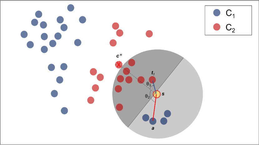
Figure 1: Proposed approach to select the samples inside the semicircle that surrounds the test sample $\bm{s}$. The dimmest area is the semicircle representation proposed for our approach. The dashed line is the distance between $\bm{s}$ and the nearest class centroid $\bm{c}^{\star}$. The solid blue solid depicts the selected nearest sample $\bm{t}_{1}$, while the solid red line depicts a sample $\bm{a}$ that is not included in the class prediction of $\bm{s}$.

As illustrated in Figure 1, instead of picking all samples inside the circle, we want to find the ones assumed to be as close as possible to the cluster of the centroid $\bm{c}^{\star}$. Furthermore, since Euclidean distance is sensitive to high-dimensional spaces, we use the Manhattan distance to avoid intensifying features with large differences in such scenarios.

Step 6 of the algorithm above regards the final prediction of the test sample $\bm{s}$ according to the following equations:

$$p_{i}(\bm{s})=\frac{\displaystyle\sum_{\forall\bm{t}\in{\cal T}\wedge\lambda(t)=\omega_{i}}{D_{M}(\bm{t}_{j},\bm{s})}^{-1}\ast W(\bm{t}_{j},\bm{c}_{i})}{\sum_{k=1}^{n}p_{k}(\bm{s})},\forall i\in{\cal Y},$$ (1)

and

$$y_{s}=\operatorname*{arg\,max}_{i}(p_{i}),\forall i=1,2,\ldots,n,$$ (2)

where $y_{s}$ is the predicted class of $s$, $\lambda(\bm{t})$ outputs the true label of sample $\bm{t}$, and $p_{i}(\bm{s})$ stands for the probability of sample $\bm{s}$ belonging to class $\omega_{i}$. We want to penalize the neighbor’s samples of $\bm{s}$ with the farthest distance to their cluster centroid. Those samples will have less impact on the final prediction of $\bm{s}$ since they are distant from their correct class group, representing possible outliers.

III Methodology

This section presents the datasets used in this study and the setup of the experiments.

III-A Datasets

The experiments were performed over 11 public datasets from the UCI Machine Learning  repository. The datasets include binary and multiclass labels, variation in the number of features, and numerical features only. The latter aspect is more concerned with avoiding the encoding of categorical features. The description of the datasets is presented in Table I.

TABLE I: DESCRIPTION OF THE DATASETS USED IN THE EXPERIMENTS.

Dataset	Description
	Samples	Features	Classes
Blood Transfusion (BT)	748	4	2
Breast Cancer Diagnostic (BCD)	569	30	2
Breast Cancer Original (BCO)	699	10	2
Forest Type (FT)	523	27	4
HCV data (HCV)	615	13	5
Indian Liver (IL)	583	10	2
Mammographic Mass (MM)	961	6	2
Somerville Hapiness (SH)	143	6	2
SPECT Heart (SPTH)	267	44	2
Urban Land Cover (ULC)	168	148	9
Wine (WN)	178	13	3

III-B Experimental Setup

The PL-$k$NN model  and all baselines were implemented using Python 3.6. We rely on Algorithm 1 presented in Ayyad et al. [5] to develop the source code of SMKNN and LMKNN. The datasets were divided into 20 folds of training, validation, and testing sets considering a proportion of 70%, 15%, and 15%, respectively. Apart from the statistical analysis between the baselines and the proposed classifier’s results, the splitting strategy also enables the optimization of the $k$ value employed by the standard $k$-NN classifier using the training and validation sets. The best $k$ was computed from a range between 1 and 50 to find the value that maximizes the accuracy over the validation set. Also, we used the average accuracy and F1-Score to assess the PL-$k$NN effectiveness. Finally, the Wilcoxon signed-rank [16] test with 5% of significance was employed to evaluate the statistical similarity among PL-$k$NN and the baselines over each dataset. Besides, a post hoc analysis was also conducted using the Nemenyi test [17] with $\alpha=0.05$ to expose the critical difference (CD) among all techniques.

IV Experiments

This section compares the PL-$k$NN with $k$-NN, SMKNN, and LMKNN. Despite intending the gene classification task, SMKNN and LMKNN are easily adaptable to other contexts due to the cluster analysis, which is intrinsic to any data distribution. Moreover, both techniques work similarly to PL-$k$NN, particularly the SMKNN variant, which is the base of our model, thus constituting a reasonable comparison in public datasets.

For the sake of comparison, the best value for the $k$-NN model was configured using the optimization step described in Section III. Notice the most accurate average F1-Score is in bold, while similar results according to the Wilcoxon signed-rank test with $5\%$ of significance are underlined for all classifiers. The F1-Score was particularly preferable to assess the model effectiveness because of the imbalanced class distribution of some datasets used in the experiments, such as the Forest Type, HCV data, and SPECT Heart.

Table II presents the average results where the proposed model obtained the best F1-Score in seven out of eleven datasets. The proposed model showed similar and higher F1-Score values for the Blood Transfusion, Forest Type, HCV, Indian Liver, Mammographic, Somerville Happiness, SPECT Heart, Urban Land Cover, and Wine datasets. Even when the proposed model showed inferior results, the average metrics were almost equivalent as observed in the Forest Type and Mammographic Mass datasets. Furthermore, the proposed method surpassed the effectiveness obtained by SMKNN and LMKNN in cases where $k$-NN showed the best F1-Score and the results were statistically different. Notice such behavior presented by Breast Cancer Diagnostic and Breast Cancer Original datasets. Besides, it is worth noting the low performance of LMKNN over some datasets such as Forest Type, HCV, Indian Liver, and Urban Land Cover, which probably relates to its mechanism that assumes a more significant number of neighbors while computing the radius of the circle.

TABLE II: AVERAGE RESULTS OBTAINED BY EACH CLASSIFIER.

Dataset	Method	Measure
		Accuracy	F1-Score
BT	$k$-NN	0.7844 ± 0.0270	0.3806 ± 0.0934
	LMKNN	0.7594 ± 0.0250	0.3192 ± 0.0786
	SMKNN	0.7585 ± 0.0319	0.4217 ± 0.0944
	PL-$k$NN	0.7121 ± 0.0499	0.4439 ± 0.0848
BCD	$k$-NN	0.9553 ± 0.0254	0.9373 ± 0.0371
	LMKNN	0.9076 ± 0.0221	0.8595 ± 0.0376
	SMKNN	0.9247 ± 0.0212	0.8898 ± 0.0338
	PL-$k$NN	0.9406 ± 0.0176	0.9153 ± 0.0266
BCO	$k$-NN	0.9648 ± 0.0195	0.9479 ± 0.0300
	LMKNN	0.7743 ± 0.0278	0.5073 ± 0.0896
	SMKNN	0.9481 ± 0.0196	0.9208 ± 0.0306
	PL-$k$NN	0.9510 ± 0.0198	0.9255 ± 0.0310
FT	$k$-NN	0.8692 ± 0.0554	0.8616 ± 0.0614
	LMKNN	0.5256 ± 0.0290	0.3014 ± 0.0219
	SMKNN	0.8513 ± 0.0437	0.8397 ± 0.0557
	PL-$k$NN	0.8538 ± 0.0424	0.8494 ± 0.0494
HCV	$k$-NN	0.9136 ± 0.0170	0.4839 ± 0.1036
	LMKNN	0.8696 ± 0.0000	0.1860 ± 0.0000
	SMKNN	0.9071 ± 0.0199	0.4843 ± 0.1245
	PL-$k$NN	0.9092 ± 0.0147	0.4985 ± 0.1197
IL	$k$-NN	0.6897 ± 0.0378	0.1958 ± 0.1020
	LMKNN	0.7126 ± 0.0178	0.0723 ± 0.0643
	SMKNN	0.7121 ± 0.0361	0.2558 ± 0.0886
	PL-$k$NN	0.7121 ± 0.0294	0.3336 ± 0.0635
MM	$k$-NN	0.8045 ± 0.0330	0.7855 ± 0.0380
	LMKNN	0.7740 ± 0.0276	0.7627 ± 0.0276
	SMKNN	0.7823 ± 0.0282	0.7666 ± 0.0294
	PL-$k$NN	0.7785 ± 0.0302	0.7689 ± 0.0301
SH	$k$-NN	0.5476 ± 0.1190	0.4667 ± 0.1844
	LMKNN	0.6119 ± 0.0695	0.5106 ± 0.1338
	SMKNN	0.5667 ± 0.0877	0.4601 ± 0.1212
	PL-$k$NN	0.6167 ± 0.0714	0.5177 ± 0.1266
SPTH	$k$-NN	0.8087 ± 0.0483	0.3797 ± 0.1890
	LMKNN	0.7587 ± 0.0582	0.5150 ± 0.1033
	SMKNN	0.7163 ± 0.0644	0.4665 ± 0.0905
	PL-$k$NN	0.7675 ± 0.0507	0.5320 ± 0.0702
ULC	$k$-NN	0.7782 ± 0.0265	0.7671 ± 0.0351
	LMKNN	0.5515 ± 0.0390	0.3470 ± 0.0375
	SMKNN	0.7728 ± 0.0359	0.7654 ± 0.0393
	PL-$k$NN	0.8005 ± 0.0377	0.7946 ± 0.0402
WN	$k$-NN	0.9519 ± 0.0424	0.9530 ± 0.0424
	LMKNN	0.9481 ± 0.0429	0.9508 ± 0.0421
	SMKNN	0.9537 ± 0.0368	0.9545 ± 0.0370
	PL-$k$NN	0.9630 ± 0.0310	0.9640 ± 0.0308

Besides the Wilcoxon signed-rank test, we also employ the Nemenyi test to provide an overall statistical analysis. The method examines the critical difference among all techniques to plot the method’s average rank in a horizontal bar (see Figure 2). Notice lower ranks denote better performance, and the methods connected are similar in terms of statistical significance. One can notice the best result attained by the PL-$k$NN model. Also, the proposed approach achieved statistical similarity and better performance compared to the baseline techniques.

Figure 2: Nemenyi test computed for all techniques.

V Conclusions and Future Works

This paper presented PL-$k$NN, a novel approach for automatically determining the number of nearest neighbors for the $k$-NN classifier. Experiments over 11 datasets showed the competitive results obtained from the proposed model according to statistical analysis applied to all the baselines used for comparison. Besides, the Nemenyi test also confirms the statistical similarity of the PL-$k$NN results with the ones obtained by the standard $k$-NN classifier configured with the best $k$ value. Regarding future studies, we intend to identify the regions in which the entire circle may be necessary to provide more neighboring samples to increase the prediction accuracy. Furthermore, we also plan to extend PL-$k$NN to regression analysis.

References

- [1] M. V. Menezes, L. C. Torres, and A. P. Braga, “Width optimization of RBF kernels for binary classification of support vector machines: A density estimation-based approach,” Pattern Recognition Letters, vol. 128, pp. 1–7, 2019.
- [2] K. M. C. Mohammed, S. SrinivasKumar, and G. Prasad, “Defective texture classification using optimized neural network structure,” Pattern Recognition Letters, 2020.
- [3] J. P. Papa, A. X. Falcão, and C. T. N. Suzuki, “Supervised pattern classification based on optimum-path forest,” International Journal of Imaging Systems and Technology, vol. 19, no. 2, pp. 120–131, 2009.
- [4] J. L. Bentley, “Multidimensional binary search trees used for associative searching,” Communications of the ACM, vol. 18, no. 9, p. 509–517, 1975.
- [5] S. M. Ayyad, A. I. Saleh, and L. M. Labib, “Gene expression cancer classification using modified K-Nearest Neighbors technique,” BioSystems, vol. 176, pp. 41–51, 2019.
- [6] K. J. Luken, R. P. Norris, and L. A. Park, “Preliminary Results of Using k-nearest-neighbor Regression to Estimate the Redshift of Radio-selected Data Sets,” Publications of the Astronomical Society of the Pacific, vol. 131, no. 1004, p. 108003, 2019.
- [7] L. Zhong, L. Lin, Z. Lu, Y. Wu, Z. Lu, M. Huang, W. Yang, and Q. Feng, “Predict CT image from MRI data using KNN-regression with learned local descriptors,” in 2016 IEEE 13th International Symposium on Biomedical Imaging (ISBI). IEEE, 2016, pp. 743–746.
- [8] M. Farshad and J. Sadeh, “Accurate single-phase fault-location method for transmission lines based on k-nearest neighbor algorithm using one-end voltage,” IEEE Transactions on Power Delivery, vol. 27, no. 4, pp. 2360–2367, 2012.
- [9] M. Murugappan, “Human emotion classification using wavelet transform and KNN,” in 2011 International Conference on Pattern Analysis and Intelligence Robotics, vol. 1. IEEE, 2011, pp. 148–153.
- [10] L. A. Passos and J. P. Papa, “A metaheuristic-driven approach to fine-tune deep boltzmann machines,” Applied Soft Computing, p. 105717, 2019.
- [11] A. S. Wicaksono and A. A. Supianto, “Hyper Parameter Optimization using Genetic Algorithm on Machine Learning Methods for Online News Popularity Prediction,” International Journal of Advanced Computer Science and Applications, vol. 9, no. 12, pp. 263–267, 2018.
- [12] P. Ling, D. Gao, X. Zhou, Z. Huang, and X. Rong, “Improve the diagnosis of atrial hypertrophy with the local discriminative support vector machine,” Bio-Medical Materials and Engineering, vol. 26, no. s1, pp. S1813–S1820, 2015.
- [13] X. Zhang and Q. Song, “Predicting the number of nearest neighbors for the k-nn classification algorithm,” Intelligent Data Analysis, vol. 18, no. 3, pp. 449–464, 2014.
- [14] H. Singh, A. Desai, and V. Pudi, “PAGER: Parameterless, Accurate, Generic, Efficient kNN-based Regression,” in International Conference on Database and Expert Systems Applications. Springer, 2010, pp. 168–176.
- [15] A. Desai, H. Singh, and V. Pudi, “GEAR: Generic, Efficient, Accurate kNN-based Regression,” in International Conference on Knowledge Discovery and Information Retrieval (KDIR), 2010, pp. 1–13.
- [16] F. Wilcoxon, “Individual comparisons by ranking methods,” Biometrics Bulletin, vol. 1, no. 6, pp. 80–83, 1945.
- [17] P. Nemenyi, Distribution-free Multiple Comparisons. Princeton University, 1963.