STD: Stable Triangle Descriptor for 3D place recognition

Abstract

In this work, we present a novel global descriptor termed stable triangle descriptor (STD) for 3D place recognition. For a triangle, its shape is uniquely determined by the length of the sides or included angles. Moreover, the shape of triangles is completely invariant to rigid transformations. Based on this property, we first design an algorithm to efficiently extract local key points from the 3D point cloud and encode these key points into triangular descriptors. Then, place recognition is achieved by matching the side lengths (and some other information) of the descriptors between point clouds. The point correspondence obtained from the descriptor matching pair can be further used in geometric verification, which greatly improves the accuracy of place recognition. In our experiments, we extensively compare our proposed system against other state-of-the-art systems (i.e., M2DP, Scan Context) on public datasets (i.e., KITTI, NCLT, and Complex-Urban) and our self-collected dataset (with a non-repetitive scanning solid-state LiDAR). All the quantitative results show that STD has stronger adaptability and a great improvement in precision over its counterparts. To share our findings and make contributions to the community, we open source our code on our GitHub: github.com/hku-mars/STD.

I Introduction

Place recognition refers to the problem of detecting if two measurements of the sensor (e.g., camera image, LiDAR point cloud) are collected in the same scene. It is a fundamental problem in a variety of robotic applications, such as loop detection in simultaneous localization and mapping (SLAM)[1, 2, 3], global re-localization in prior maps [4, 5], and maps merging in multi-robot systems [6]. Many vision-based SLAM systems [7, 8, 9, 10, 11] have been proposed due to the widespread use of cameras. However, these loop detection methods are difficult to deal with the strong variation caused by illumination, appearance, or viewpoint changes. On the other hand, Light Detection and Ranging sensor (LiDAR) is invariant to illumination and appearance change as it can directly obtain the structural information of the environment. The emergence of low-cost and high-performance LiDARs has further increased the use of LiDAR in robotics [12, 13, 14, 15].

Generally, an efficient LiDAR-based place recognition solution should satisfy the following requirements. First, the solution is required to achieve both rotation and translation invariance regardless of the viewpoint changes. Second, the solution should better provide a relative pose. A good initial pose estimation allows the subsequent registration algorithm to converge faster and more accurate. Third, the method should be robust to different LiDAR point cloud densities and environments since the sparsity of LiDAR point cloud varies with distance, scene, and LiDAR types.

In order to achieve the above performance, in this paper, we develop a new descriptor termed stable triangle descriptor (STD), which encodes any three key points in the scene by a triangle. Compared with polygons used in other descriptors, the triangle is more stable because the shape of the triangle is uniquely defined given the length of the sides (or included angles). Compared with local descriptors around key points, the shape of a triangle is completely rotation and translation invariant. To extract key points for triangle descriptors, we perform point cloud projection on the plane and extract key points on the boundary, then form the key points into triangles. Matches are made based on the similarity of triangles. A typical place recognition case with STD is shown in Fig. 1, which successfully recognizes two point clouds collected at opposite view angles in the same place. Specifically, our contributions are as follows:

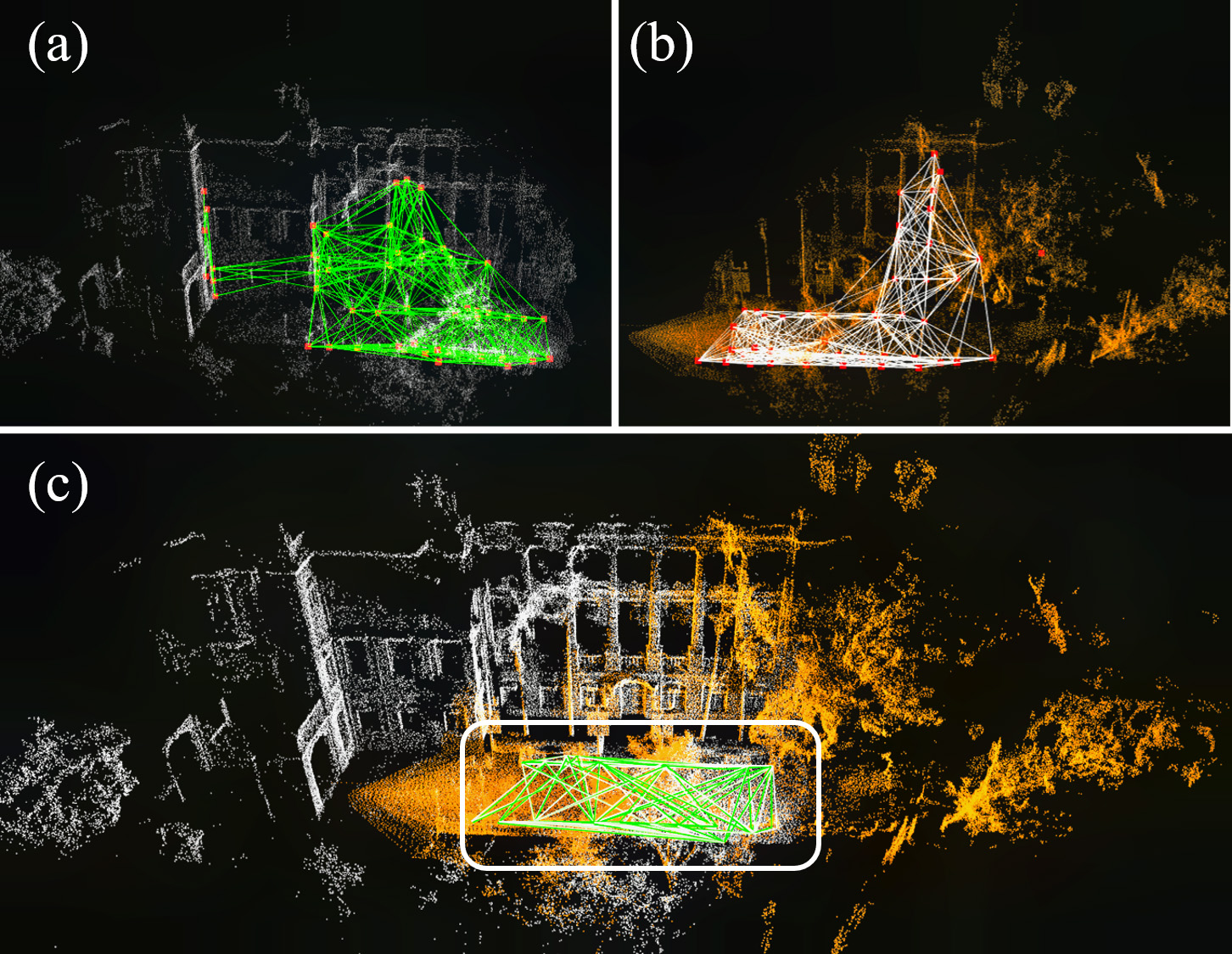
Figure 1: (a) shows the stable triangle descriptor (STD) extracted from a query point cloud. (b) shows the STD extracted from a historical point cloud. In (c), an example of STD matching between these two frames of the point cloud. The correctly matched STD descriptors are indicated by white box, and the point clouds are registered by the poses provided by the STD. These two frames of point clouds are collected by a small FOV LiDAR (Livox Avia) moving in opposite directions, resulting in a low point cloud overlap and drastic viewpoint change (See our accompanying video on YouTube: youtu.be/O-9iXn1ME3g).

• We design a triangle descriptor (see Fig. 3), a six-dimension vector consisting of the length of three triangle sides and the angles between the normal vectors of the adjacent plane attached to each triangle vertex. The descriptor is completely invariant to rotation and translation while maintaining a high degree of distinguishability.

• We propose a fast key point extraction method based on keyframes. In order to represent the structural information of the scene, we project the point cloud at the plane boundary and extract key points therein, which will form triangle descriptors with adjacent key points.

• We evaluate our algorithm under multiple types of scenarios (urban, indoor, and unstructured environments) and different LiDAR data (conventional spinning LiDARs and solid state LiDARs). Sufficient experimental results verify the effectiveness of our method.

• To share our findings and make contributions to the community, let our readers can quickly reproduce our work in their follow-up research, we make our codes publicly available on our GitHub: github.com/hku-mars/STD.

II Related Works

Place recognition in 3D data is a key problem for robot localization and has been addressed in different approaches. According to the principle of the methods, we have divided the existing work into the following three categories: (i) local descriptor based on point features. (ii) global descriptor based on appearance (iii) learning-based method.

Inspired by the place recognition solution in robotic vision, Bastian[16] transforms a given 3D scan data into a range image, then extracts point features from the range image and performs score matching for 3D scan data based on point features. Bosse and Zlot [17] extract key points directly on 3D data, then use the Gestalt Descriptor that encodes each key point’s neighborhood and calculate the voting matrix for place recognition. Apart from the Gestalt descriptors, some other descriptors, such as PFH [18], SURFs [19], or SHOT [20], are also used in a similar framework. However, these local descriptors are sensitive to the density and noise of the LiDAR point clouds and are not invariant to rotation or translation of the viewpoint.

Global descriptors prefer to use the appearance information of the point cloud. Magnusson et al. [21] first divide the point cloud into overlapping grids, then compute the shape properties of each cell by normal distribution transform, and finally combines them into a matrix of surface shape histograms. He et al. propose M2DP [22], which is generated by projecting a 3D point cloud to multiple 2D planes and generating a high dimensional compact global representation. Giseop Kim and Ayoung Kim [23] propose scan Context, a 2D descriptor based on the height of the surrounding structures. V. Nardari et al. [24] propose a polygon descriptor to achieve place recognition in the forest environment. Jiang et al [25] propose a triangle feature-based descriptor for 2D SLAM. In short, these global descriptors make use of the appearance information (surface flatness and orientation, height, and so on) of the scene.

In contrast with the local descriptors, global descriptors are more robust against noise and resolution changes, but they still struggle with the change of viewpoints. Therefore, some other works attempt to use deep learning for 3D place recognition tasks. SegMap [26] achieves place recognition by matching semantic features. OverlapNet [27] proposes a deep neural network to achieve overlap calculation and relative yaw angle estimates between pairs of 3D scans. These learning-based approaches all require a training step and use GPU acceleration.

Our proposed descriptor, stable triangle descriptor, is a global descriptor consisting of three key points. The triangle descriptors are extracted within a keyframe and describe the relative distribution of key points in the frame. Compared with other global descriptors [21, 22, 23], our descriptor has stronger rotation and translation invariance. Compared with the polygon descriptor [24, 25], our descriptor is extracted directly in 3D space, and uses the most recognizable and invariable triangle among polygons, while [24, 25] extracts polygon descriptors in 2D space. In addition, our descriptor can provide pose estimation with full degrees of freedom, which can greatly reduce the registration time while ensuring the registration accuracy.

III Methodology

In this section, we describe how to extract the stable triangle descriptor from a point cloud. Next, we introduce how to build the descriptor dictionary and how to select loop candidates. Finally, RANSAC-based loop detection and geometric verification are proposed for a complete loop detection pipeline. The overall pipeline of our method is depicted in Fig. 3.

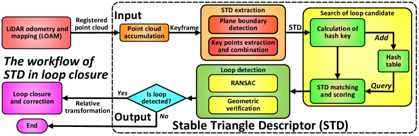
Figure 2: Workflow of our algorithm. Our method computes the triangle descriptors from keyframes. Then a hash table is used to serve as the database of our descriptors for quick store and match. Frames with the top 10 descriptor matching scores will be selected as candidates. The loop candidate is regarded as a valid loop once passing the geometric verification. The relative transformation between the loop frame and candidate frame will also be obtained as the loop is triggered.

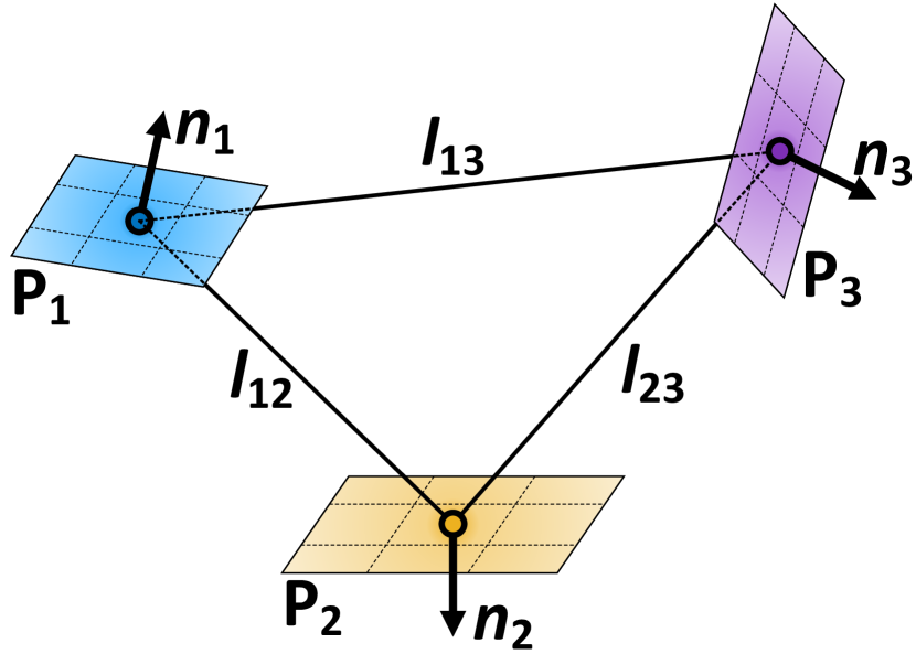
Figure 3: A standard triangle descriptor. Each vertex $\mathbf{p}_{1},\mathbf{p}_{2},\mathbf{p}_{3}$ corresponds to a adjacent plane. $\mathbf{n}_{1},\mathbf{n}_{2},\mathbf{n}_{3}$ are the normal vector to the adjacent planes. Vertices are arranged according to $l_{12}\leq l_{23}\leq l_{13}$.

III-A Stable Triangle Descriptor

Inspired by [26], to improve the stability of segmentation, we perform loop detection on keyframes, which have points accumulated from a few consecutive scans and hence have increased point cloud density regardless of the specific LiDAR scanning pattern. Specifically, we use a LiDAR odometer [28] to register each new incoming point cloud into the current keyframe. A new keyframe will be created when the number of sub-frames accumulates to a certain number. When given a keyframe of the point cloud, we first perform plane detection by region growing. Specifically, we divide the entire point cloud into voxels of given sizes (e.g., 1m). Each voxel contains a group of points $\mathbf{p}_{i}\ (i=1,...,N)$; we then calculate the point covariance matrix $\mathbf{\Sigma}$:

$$\bar{\mathbf{p}}=\frac{1}{N}\sum_{i=1}^{N}\mathbf{p}_{i};\quad\mathbf{\Sigma}=\frac{1}{N}\sum_{i=1}^{N}(\mathbf{p}_{i}-\bar{\mathbf{p}})(\mathbf{p}_{i}-\bar{\mathbf{p}})^{T};$$ (1)

Let $\lambda_{k}$ denote the $k$-th largest eigenvalue of matrix $\mathbf{\Sigma}$. The plane criterion principle is:

$$\lambda_{3}<\sigma_{1}~{}\text{and}~{}\lambda_{2}>\sigma_{2}$$ (2)

where $\sigma_{1}$ and $\sigma_{2}$ are pre-set hyperparameters. By this criterion, we can check whether the points in a voxel form a plane and if so, the voxel is called a plane voxel. Then, we initialize a plane with any plane voxel and grow the plane by searching for its neighboring voxels. If the neighboring voxels are the same planes (has the same plane normal direction with a distance below a threshold), they are added to the plane under growing. Otherwise, if the neighboring voxel is not on the same plane, it is added to a list of boundary voxels for the plane under growing. The above growing process repeats until all the added neighboring voxels are expanded, or boundary voxels are reached (see Fig. 4).

With the boundary voxels, we project their contained points to the respective plane (see Fig. 5(a) and Fig. 5(b)). For each plane, we create an image where the image plane coincides with the plane and each pixel represents the maximum distance of points contained in boundary voxels of the plane. Then, we select a point, which has the largest pixel value in its $5*5$ neighborhood, as a key point (see Fig. 5(c)). Each extracted key point corresponds to a 3D point in the input point cloud and could be attached with the normal of the plane it is extracted from.

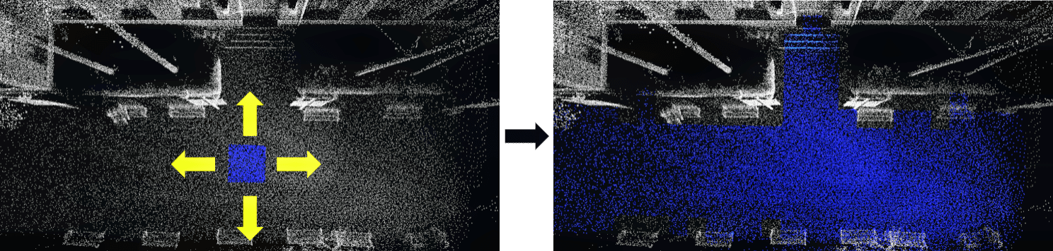
Figure 4: Plane expand process

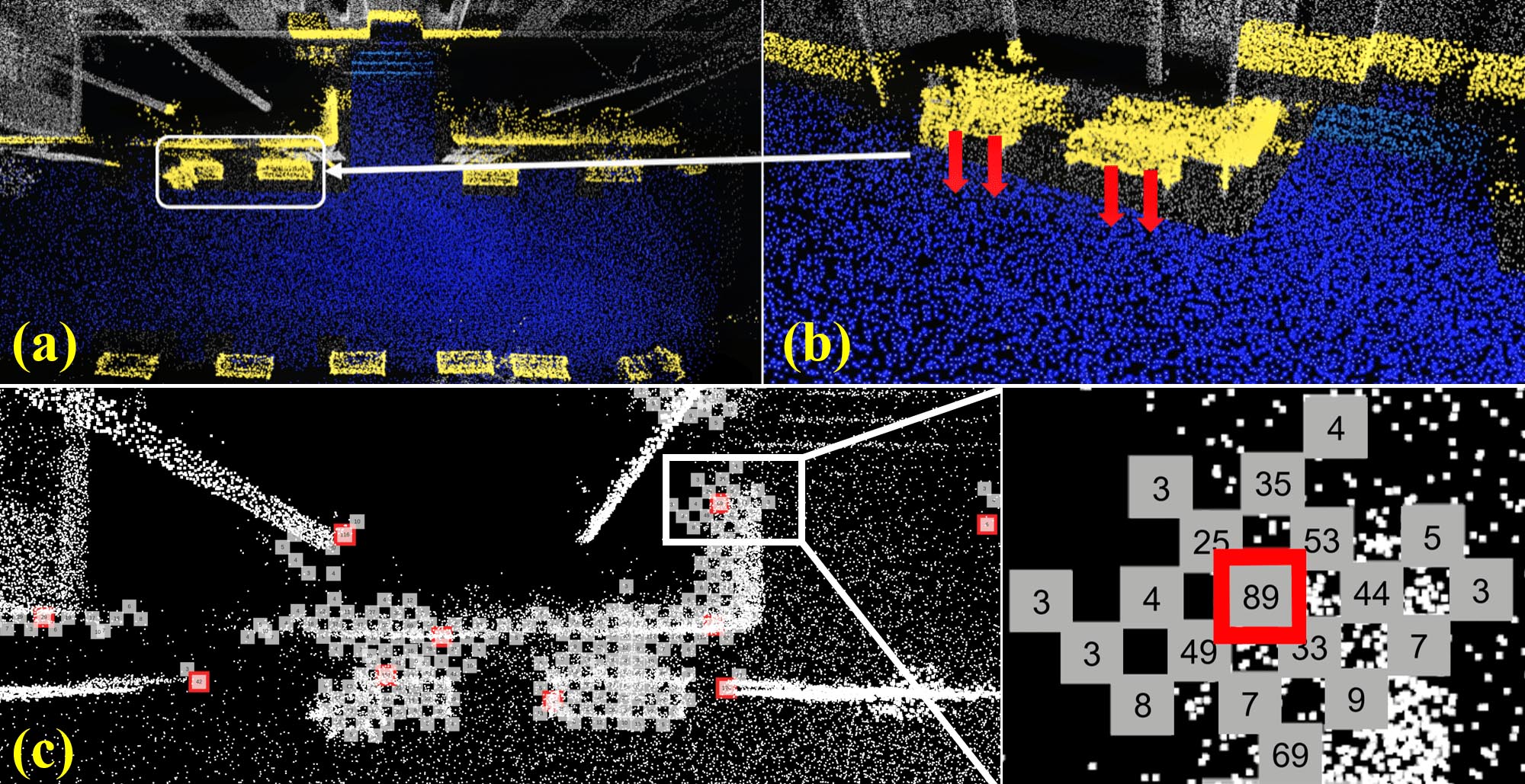
Figure 5: (a) Points in boundary voxels are colored in yellow. (b) The points are projected onto the adjacent planes (blue points). (c) The plane image where each pixel represents the maximum distance (in cm) of points in boundary voxels to the plane. If a point has the maximum pixel value in its 5*5 neighborhood, it will be considered as the key points (red points).

With the extracted key points in a keyframe, we build a $k$-D tree and search 20 near neighbor points for each point to form the triangle descriptor. Redundant descriptors with the same side length will be eliminated. Each triangle descriptor contains three vertices, $\mathbf{p}_{1}$, $\mathbf{p}_{2}$ and $\mathbf{p}_{3}$, with projection normal vectors $\mathbf{n}_{1}$, $\mathbf{n}_{2}$ and $\mathbf{n}_{3}$. Besides, the vertices of the triangle are arranged according to the rule of side length in ascending order (see Fig. 3). We summarize that a triangle descriptor $\boldsymbol{\Delta}$ has the following contents:

• $\mathbf{p}_{1}$, $\mathbf{p}_{2}$, $\mathbf{p}_{3}$: three vertices,

• $\mathbf{n}_{1}$, $\mathbf{n}_{3}$, $\mathbf{n}_{3}$: three projection normal vectors,

• $l_{12}$, $l_{23}$, $l_{13}$: three sides, and $l_{12}\leq l_{23}\leq l_{13}$,

• $\mathbf{q}$: the centriod of the triangle,

• $k$: the frame number corresponding to the descriptor.

In addition to descriptors, we will also save all $n$ planes ${\Pi}=(\boldsymbol{\pi}_{1},\boldsymbol{\pi}_{2},\ldots,\boldsymbol{\pi}_{n})$ extracted from this keyframe for the following geometrical verification step.

III-B Search of Loop Candidates

Since hundreds of descriptors can be extracted from a keyframe, to quickly query and match descriptors, we use a Hash table to store all descriptors. We use six attributes with rotation and translation invariance in the descriptor to compute the hash key, which are side lengths $l_{12}$, $l_{23}$, $l_{13}$, and the dot product of the normal projection vector $\mathbf{n}_{1}\cdot\mathbf{n}_{2}$, $\mathbf{n}_{2}\cdot\mathbf{n}_{3}$, $\mathbf{n}_{1}\cdot\mathbf{n}_{3}$ respectively. Descriptors with all six similar attributes will have the same hash key and hence be stored in the same container. For a query keyframe, we extract all its descriptors as detailed in Sec. III-A. For each descriptor $\boldsymbol{\Delta}_{i}$, we calculate its hash key, locate it to the corresponding container in the Hash table and vote once for the keyframes that have a descriptor in this container. The matching process finishes when all descriptor $\boldsymbol{\Delta}_{i}$ in the query keyframe are processed. keyframes with the top 10 votes will be selected as candidates with matched descriptors saved for the use of the loop detection step.

Remark 1: Since boundary points are projected to the plane extracted from the 3D point cloud instead of from the range image, such as in [16], the extracted key point is invariant to the view angle change. Moreover, the six descriptor attributes are also invariant to any rigid transformation. Hence, the overall method is rotation and translation invariance.

Remark 2: Thanks to the ordering of the triangle side length and the stability of the triangle, two triangles are assured to be the same if and only if the length of their ordered sides are equal, without enumerating the side correspondence.

III-C Loop Detection

When given a loop candidate keyframe, we perform geometrical verification to eliminate the false detection due to incorrect descriptor matching pairs. Since the shape of the triangle is uniquely determined after the side length is determined, once $\mathbf{\Delta}_{a}$ is matched to $\mathbf{\Delta}_{b}$, their vertices $(\mathbf{p}_{a_{1}},\mathbf{p}_{a_{2}},\mathbf{p}_{a_{3}})$ and $(\mathbf{p}_{b_{1}},\mathbf{p}_{b_{2}},\mathbf{p}_{b_{3}})$ naturally match. Then with this point correspondence, we can easily calculate the relative transformation $\mathbf{T}=(\mathbf{R},\mathbf{t})$ between these two keyframes through Singular Value Decomposition (SVD):

$$\mathbf{H}=\sum\nolimits_{i=1}^{3}(\mathbf{p}_{a_{i}}-\mathbf{q}_{a})(\mathbf{p}_{b_{i}}-\mathbf{q}{{}_{b}})$$ (3)

$$[\mathbf{U},\ \mathbf{S},\ \mathbf{V}]=\mathtt{SVD}(\mathbf{H})$$

$$\mathbf{R}=\mathbf{VU}^{T},\ \mathbf{t}=-\mathbf{R}*\mathbf{q}_{a}+\mathbf{q}_{b}.$$

To increase the robustness, we use RANSAC[29] to find the transformation that maximizes the number of correctly matched descriptors.

Based on this transformation, we calculate the plane overlap between the current frame and the candidate frame for geometrical verification. Let a center point $\mathbf{g}$ and a normal vector $\mathbf{u}$ represent a plane $\boldsymbol{\pi}$ in a voxel. Denote the plane group of the current frame be ${}^{B}\Pi=[({}^{B}\mathbf{g}_{1},{}^{B}\mathbf{u}_{1}),...({}^{B}\mathbf{g}_{n},{}^{B}\mathbf{u}_{n})])$, the plane group of the candidate frame be ${}^{C}\Pi=[({}^{C}\mathbf{g}_{1},{}^{C}\mathbf{u}_{1}),...({}^{C}\mathbf{g}_{m},{}^{C}\mathbf{u}_{m})])$, and the rigid-body transformation be ${}^{C}_{B}\mathbf{T}=({}^{C}_{B}\mathbf{R},{}^{C}_{B}\mathbf{t})\in SE(3))$, where $n$ is the number of planes in the current frame and $m$ is the number of planes in the candidate frame. We construct a $k$-D tree ($k=3$) with the center points $({}^{C}\mathbf{g}_{1},{}^{C}\mathbf{g}_{2},...,{}^{C}\mathbf{g}_{m})$ from the ${}^{C}\Pi$. Then for each plane center point ${}^{B}\mathbf{g}_{i}\ (i=1,2,...,n)\in{}^{B}\Pi$. We first transform ${}^{B}\mathbf{g}_{i}$ by the transformation ${}^{C}_{B}\mathbf{T}$, then search a nearest point ${}^{C}\mathbf{g}_{j}$ in the $k$-D tree, and judge whether the two planes coincide by the difference in normal vector and the point-to-plane distance:

$$\|{}^{C}_{B}\mathbf{R}{}^{B}\mathbf{u}_{i}-{}^{C}\mathbf{u}_{j}\|_{2}<\sigma_{n}$$ (4)

$${}^{C}\mathbf{u}_{j}^{T}({}^{C}_{B}\mathbf{T}{}^{B}\mathbf{g}_{i}-{}^{C}\mathbf{g}_{j})<\sigma_{d},$$

where $\sigma_{n}$ and $\sigma_{d}$ are preset hyperparameters to determine whether planes overlap or not. If a pair of planes satisfies the normal vector and point-to-distance constraints in equation (4), the pair of planes are coinciding. After checking all planes of the current frame, we calculate the percent of plane coincidence ($N_{c}$):

$$N_{c}=\frac{N_{\mathtt{coincide}}}{N_{\mathtt{sum}}}\times 100\%,$$ (5)

where $N_{\mathtt{coincide}}$ is the number of coninciding planes and $N_{\mathtt{sum}}$ is the number of all planes of the current frame. If the $N_{c}$ of the current frame and the candidate frame exceeds a certain threshold $\sigma_{\mathtt{pc}}$, we finally consider it to be a valid loop detection. It is worth noting that geometric verification based on planes is much more efficient than the ICP-based methods since the number of planes is much less than the number of point clouds. Besides, we can further optimize the normal vector difference and point-to-plane distance in equation (4) to obtain a more accurate transformation for loop correction, which can be easily implemented using Ceres-Solver[30]. We defined this optimization process as STD-ICP and the performance of STD-ICP will be verified in experiments.

IV Experiments

In this section, to verify the effectiveness, robustness and adaptability of our method, we evaluate our algorithm in different scenarios (urban, indoor and unstructured environments) with different types of LiDAR (mechanical spinning LiDARs and solid state LiDARs). In each experiment, we compare our method with state-of-the-art counterparts. All experiments are carried out on the same system with an Intel i7-11700k @ 3.6 $\rm GHz$ with 16 $\rm{GB}$ memory.

IV-A Benchmark Evaluation

In this experiment, we evaluate our method on the open urban dataset including KITTI odometry dataset [31], NCLT dataset [32] and Complex Urban dataset [33]. All data were collected in urban environments using mechanical spinning LiDARs with different scanning lines. We compare our method with two other global descriptors: Scan Context [23] and M2DP [22]. We accumulate every 10 frames into a keyframe for these datasets. If the ground truth pose distance between the query keyframe and the matched keyframe is less than 20m, the detection is considered a true positive.

For the implementation, we run our algorithm on all datasets with the same parameters, where the voxel size is 1m, the plane judgement threshold $\sigma_{1}$ and $\sigma_{2}$ are 0.01 and 0.05, respectively, the normal different threshold $\sigma_{n}$ is 0.2 and the point-to-plane distance threshold $\sigma_{d}$ is 0.3m. For Scan Context [23] and M2DP [22], we directly use the results presented in the original paper [23].

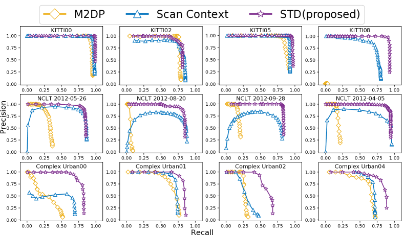
Figure 6: Precision-Recall curves on KITTI, NCLT and Complex Urban datasets .

IV-A1 Precision-Recall Evaluation

We evaluate the performance of STD by the precision-recall curve when vary plane coincide threshold $\sigma_{\mathtt{pc}}$ as shown in Fig. 6. Since Scan Context-50 performs better than Scan Context-10 in most scenarios, we only show the result from Scan Context-50. From the results, STD outperforms Scan Context and M2DP in almost all datasets. As stated in [23], their method does not perform as well in narrow scenarios where variation in vertical height is less significant. However, our method is not limited to the height of the scene, and a successful loop detection in such a scene is shown in Fig. 7 (a). Our method performs poorly only when the structure or planes of the scene are particularly sparse because the key points extracted in such scenes will be scarce. A typical failure example is shown in Fig. 7 (b). Both cases are from the NCLT dataset.

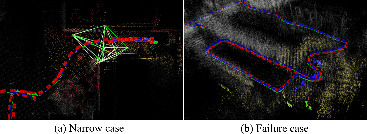
Figure 7: A challenge case in narrow scenario and a failure case of STD.

IV-A2 Run Time Evaluation

We record the computation time on KITTI00 for all methods, as shown in Fig. 9. For M2DP [22], we test with their open-sourced MATLAB code with the default parameter. For Scan Context [23], we modified their MATLAB code (add 8 Scan Context augmentations) to obtain the results in Sec. IV-A1. Point cloud downsampling with a $0.5\ m^{3}$ voxel grid is used for all methods. As shown in Fig. 9, the time consumption per frame in Scan Context and M2DP linearly increases with the number of frames in the library, while our method does not have such a linear growing trend. That is mainly due to our use of a Hash table as the database to store descriptors, which avoids building a $k$-D tree for historical descriptors like M2DP and Scan Context do. Overall, the computation time of STD is similar with M2DP, while it processing 10 times more points than M2DP. Scan Context uses augmented descriptors, which increases time consumption in both descriptor build and search loop.

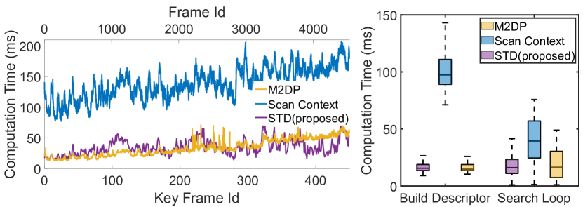
Figure 8: Time Evaluation on KITTI00

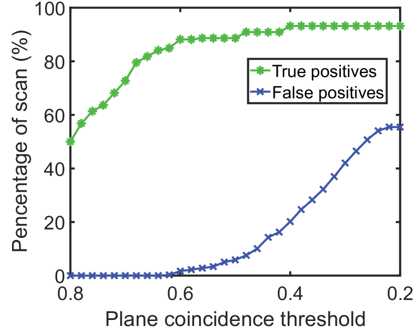
Figure 9: The effect of the plane coincidence threshold $\sigma_{\mathtt{pc}}$ on the true positive rate and false positive rate on KITTI08.

IV-A3 Plane Coincidence Threshold Selection

As can be seen from Fig. 6, Precision-Recall curves of STD always decline from precision equal to 1, mainly due to the selection of the plane coincide threshold $\sigma_{\mathtt{pc}}$. When a relatively large $\sigma_{\mathtt{pc}}$ is given, only the loop with large point cloud overlap will be selected, which is $100\%$ accurate in the urban dataset we use. When the threshold decreases, more loops with smaller overlap will be selected, introducing possible false positives. We record the true and false positive rates corresponding to different $\sigma_{\mathtt{pc}}$ of STD on Kitti08 in Fig. 9. It can be seen from the figure that $0.5\sim 0.6$ is a good trade-off value.

IV-A4 Localization Evaluation

Some other descriptors [23, 27] can estimate the yaw angle between the loop frame and the candidate frame while performing loop detection. Our proposed descriptor has further improved this function since we can provide the relative transformation of all six degrees of freedom between the loop frame and the candidate frame without extra calculation. To verify this, we conduct the experiment on the loop nodes of KITTI00. For each loop node, we set the transform relative to matched frame a random initial value uniformly drawn from a neighborhood ($\pm 5^{\circ}$ in each axis of rotation and $\pm 5$m in each axis of translation) of the ground truth value. Fig. 11 shows the error and computation time of GICP, STD and STD-ICP. STD-ICP can achieve similar accuracy as GICP with less variance in both rotation and translation. This is because STD provides a good initial value for STD-ICP, while GICP is likely to have a local optimum in loop nodes with less overlap. In addition, STD and STD-ICP take much less time than GICP, only less than $1\%$ of GICP. This is because the number of planes (hundreds) is very small compared to the size of the point cloud (more than 100K).

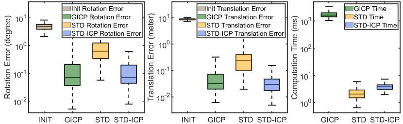
Figure 10: Pose error and computation time of GICP, STD and STD-ICP.

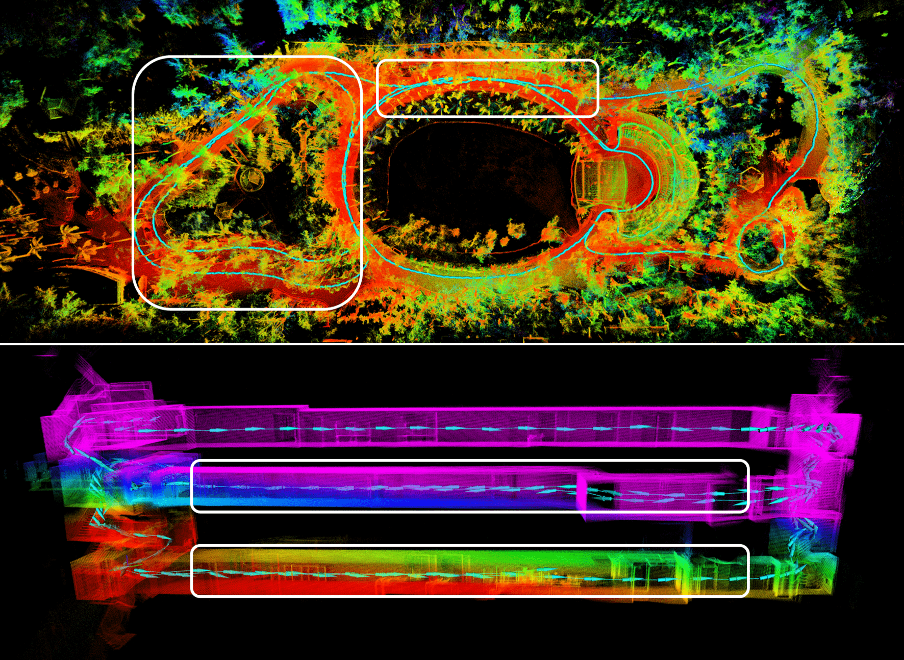
Figure 11: The fine point cloud map in park and indoor environments. Loop nodes are indicated by white boxes.

IV-B Applicability to Other Types of LiDARs

In this experiment, to evaluate the adaptability and applicability of STD in different environments and using different LiDARs, we conduct experiments with Livox series solid-state LiDARs in urban, unstructured and indoor environments. For the urban environment, we choose the KA_Urban_East dataset, which is collected by Livox Horizon LiDAR and open-sourced in LiLi-OM [34]. For the unstructured environment experiment, we collect two groups of loop data inside a park filled with trees. For the indoor environment, we collect the loop data in a multi-floor building. These two datasets are collected by Livox Avia LiDAR. Since Scan Context [23] is not compatible with Livox solid-state LiDARs, so we only compare STD with M2DP [22]. For the implementation, we use the default parameters of the available codes for M2DP [22]. For STD, the voxel size used in indoor is adjust to 0.5m while other parameters remain the same as in Sec. IV-A.

For the ground truth calculation, we first use a LiDAR-Inertial Odometry to get a rough map, then use loop detection and pose graph [35, 36] to get a fine map, which is used as the true value to select the ground truth loop nodes. Because the number of the point cloud in a single frame of Livox LiDAR is sparser than that of spinning LiDAR, we accumulate every 20 frames into a keyframe. Based on this, if the ground truth pose distance between the query keyframe and the matched keyframe is less than 20m for outdoor and 4m for indoor, the detection is considered as a true positive. We show the fine point cloud map and loop nodes for the park and indoor environments in Fig. 11.

IV-B1 Result Analysis

The Precision-Recall curves for STD and M2DP [22] are plotted in Fig. 12. From the figure, we can see that M2DP performs poorly on the Livox dataset, while STD achieves similar performance as IV-A on the Livox dataset, except indoor dataset. This is mainly because the corridors of each floor of the building are very similar, resulting in relatively low precision and recall. However, we can still provide a certain number of valid loop nodes for loop correction so that LiDAR loop closure can be applied to indoor mappings, such as multi-floor parking lots, museums, etc.

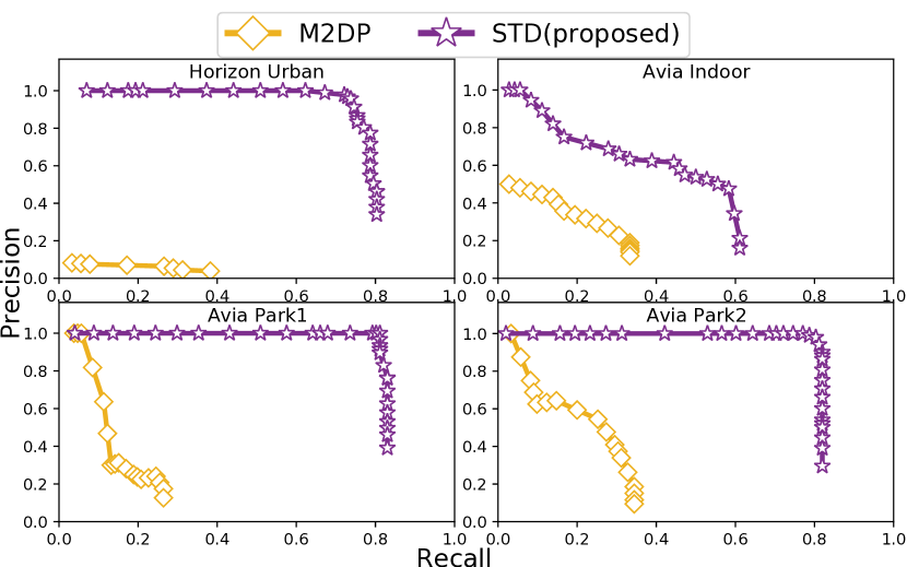
Figure 12: Precision-Recall curves on Livox LiDAR dataset.

V Conclusion

This paper proposes a triangle-based global descriptor STD. An efficient key point extraction algorithm based on plane detection and boundary projection is proposed to extract key points with geometrical features. These key points form the triangle descriptors with their neighbors. This combination greatly improves the rotation and translation invariance of descriptors. Besides, the stability and uniqueness of triangles make this descriptor naturally suitable for similarity comparison in place recognition. To speed up the querying and matching of the descriptor, we employ a Hash table as the database to store all historical descriptors, which avoids building a $k$-D tree in loop searching. Compared with other global descriptors, STD not only performs better on public datasets but also shows greater adaptability to different environments and LiDAR types.

References

- [1] J. Lin and F. Zhang, “Loamlivox: A fast, robust, high-precision lidar odometry and mapping package for lidars of small fov,” in 2020 IEEE International Conference on Robotics and Automation (ICRA). IEEE, 2020, pp. 3126–3131.
- [2] M. Labbé and F. Michaud, “Appearance-based loop closure detection for online large-scale and long-term operation,” IEEE Transactions on Robotics, vol. 29, no. 3, pp. 734–745, 2013.
- [3] J. Lin and F. Zhang, “A fast, complete, point cloud based loop closure for lidar odometry and mapping,” arXiv preprint arXiv:1909.11811, 2019.
- [4] G. Kim, B. Park, and A. Kim, “1-day learning, 1-year localization: Long-term lidar localization using scan context image,” IEEE Robotics and Automation Letters, vol. 4, no. 2, pp. 1948–1955, 2019.
- [5] B. Glocker, J. Shotton, A. Criminisi, and S. Izadi, “Real-time rgb-d camera relocalization via randomized ferns for keyframe encoding,” IEEE Transactions on Visualization and Computer Graphics, vol. 21, no. 5, pp. 571–583, 2015.
- [6] J. Lin, X. Liu, and F. Zhang, “A decentralized framework for simultaneous calibration, localization and mapping with multiple lidars,” in 2020 IEEE/RSJ International Conference on Intelligent Robots and Systems (IROS), 2020, pp. 4870–4877.
- [7] R. Mur-Artal, J. M. M. Montiel, and J. D. Tardós, “Orb-slam: A versatile and accurate monocular slam system,” IEEE Transactions on Robotics, vol. 31, no. 5, pp. 1147–1163, 2015.
- [8] T. Qin, P. Li, and S. Shen, “Vins-mono: A robust and versatile monocular visual-inertial state estimator,” IEEE Transactions on Robotics, vol. 34, no. 4, pp. 1004–1020, 2018.
- [9] J. Lin, C. Zheng, W. Xu, and F. Zhang, “R2live: A robust, real-time, lidar-inertial-visual tightly-coupled state estimator and mapping,” IEEE Robotics and Automation Letters, vol. 6, no. 4, pp. 7469–7476, 2021.
- [10] J. Lin and F. Zhang, “R3live: A robust, real-time, rgb-colored, lidar-inertial-visual tightly-coupled state estimation and mapping package,” in 2022 International Conference on Robotics and Automation (ICRA), 2022, pp. 10 672–10 678.
- [11] Y. Zhu, C. Zheng, C. Yuan, X. Huang, and X. Hong, “Camvox: A low-cost and accurate lidar-assisted visual slam system,” 2020.
- [12] W. Yang, Z. Gong, B. Huang, and X. Hong, “Lidar with velocity: Correcting moving objects point cloud distortion from oscillating scanning lidars by fusion with camera,” IEEE Robotics and Automation Letters, vol. 7, no. 3, pp. 8241–8248, 2022.
- [13] C. Yuan, X. Liu, X. Hong, and F. Zhang, “Pixel-level extrinsic self calibration of high resolution lidar and camera in targetless environments,” IEEE Robotics and Automation Letters, vol. 6, no. 4, pp. 7517–7524, 2021.
- [14] W. Xu, Y. Cai, D. He, J. Lin, and F. Zhang, “Fast-lio2: Fast direct lidar-inertial odometry,” IEEE Transactions on Robotics, 2022.
- [15] J. Lin and F. Zhang, “R3live++: A robust, real-time, radiance reconstruction package with a tightly-coupled lidar-inertial-visual state estimator,” arXiv preprint arXiv:2209.03666, 2022.
- [16] B. Steder, G. Grisetti, and W. Burgard, “Robust place recognition for 3d range data based on point features,” in 2010 IEEE International Conference on Robotics and Automation, 2010, pp. 1400–1405.
- [17] M. Bosse and R. Zlot, “Place recognition using keypoint voting in large 3d lidar datasets,” in 2013 IEEE International Conference on Robotics and Automation, 2013, pp. 2677–2684.
- [18] R. B. Rusu, N. Blodow, Z. C. Marton, and M. Beetz, “Aligning point cloud views using persistent feature histograms,” in 2008 IEEE/RSJ International Conference on Intelligent Robots and Systems, 2008, pp. 3384–3391.
- [19] H. Bay, T. Tuytelaars, and L. Van Gool, “Surf: Speeded up robust features,” in European conference on computer vision. Springer, 2006, pp. 404–417.
- [20] S. Salti, F. Tombari, and L. Di Stefano, “Shot: Unique signatures of histograms for surface and texture description,” Computer Vision and Image Understanding, vol. 125, pp. 251–264, 2014.
- [21] M. Magnusson, H. Andreasson, A. Nüchter, and A. J. Lilienthal, “Automatic appearance-based loop detection from three-dimensional laser data using the normal distributions transform,” Journal of Field Robotics, vol. 26, no. 11-12, pp. 892–914, 2009.
- [22] L. He, X. Wang, and H. Zhang, “M2dp: A novel 3d point cloud descriptor and its application in loop closure detection,” in 2016 IEEE/RSJ International Conference on Intelligent Robots and Systems (IROS). IEEE, 2016, pp. 231–237.
- [23] G. Kim and A. Kim, “Scan context: Egocentric spatial descriptor for place recognition within 3d point cloud map,” in 2018 IEEE/RSJ International Conference on Intelligent Robots and Systems (IROS). IEEE, 2018, pp. 4802–4809.
- [24] G. V. Nardari, A. Cohen, S. W. Chen, X. Liu, V. Arcot, R. A. F. Romero, and V. Kumar, “Place recognition in forests with urquhart tessellations,” IEEE Robotics and Automation Letters, vol. 6, no. 2, pp. 279–286, 2021.
- [25] B. Jiang, Y. Zhu, and M. Liu, “A triangle feature based map-to-map matching and loop closure for 2d graph slam,” in 2019 IEEE International Conference on Robotics and Biomimetics (ROBIO), 2019, pp. 2719–2725.
- [26] R. Dubé, D. Dugas, E. Stumm, J. Nieto, R. Siegwart, and C. Cadena, “Segmatch: Segment based place recognition in 3d point clouds,” in 2017 IEEE International Conference on Robotics and Automation (ICRA). IEEE, 2017, pp. 5266–5272.
- [27] X. Chen, T. Läbe, A. Milioto, T. Röhling, O. Vysotska, A. Haag, J. Behley, and C. Stachniss, “OverlapNet: Loop Closing for LiDAR-based SLAM,” in Proceedings of Robotics: Science and Systems (RSS), 2020.
- [28] C. Yuan, W. Xu, X. Liu, X. Hong, and F. Zhang, “Efficient and probabilistic adaptive voxel mapping for accurate online lidar odometry,” IEEE Robotics and Automation Letters, vol. 7, no. 3, pp. 8518–8525, 2022.
- [29] M. A. Fischler and R. C. Bolles, “Random sample consensus: a paradigm for model fitting with applications to image analysis and automated cartography,” Communications of the ACM, vol. 24, no. 6, pp. 381–395, 1981.
- [30] S. Agarwal, K. Mierle, and Others, “Ceres solver,” http://ceres-solver.org.
- [31] A. Geiger, P. Lenz, and R. Urtasun, “Are we ready for autonomous driving? the kitti vision benchmark suite,” in Conference on Computer Vision and Pattern Recognition (CVPR), 2012.
- [32] N. Carlevaris-Bianco, A. K. Ushani, and R. M. Eustice, “University of Michigan North Campus long-term vision and lidar dataset,” International Journal of Robotics Research, vol. 35, no. 9, pp. 1023–1035, 2015.
- [33] J. Jeong, Y. Cho, Y.-S. Shin, H. Roh, and A. Kim, “Complex urban dataset with multi-level sensors from highly diverse urban environments,” International Journal of Robotics Research, vol. 38, no. 6, pp. 642–657, 2019.
- [34] K. Li, M. Li, and U. D. Hanebeck, “Towards high-performance solid-state-lidar-inertial odometry and mapping,” IEEE Robotics and Automation Letters, vol. 6, no. 3, pp. 5167–5174, 2021.
- [35] M. Kaess, A. Ranganathan, and F. Dellaert, “isam: Incremental smoothing and mapping,” IEEE Transactions on Robotics, vol. 24, no. 6, pp. 1365–1378, 2008.
- [36] M. Kaess, H. Johannsson, R. Roberts, V. Ila, J. J. Leonard, and F. Dellaert, “isam2: Incremental smoothing and mapping using the bayes tree,” The International Journal of Robotics Research, vol. 31, no. 2, pp. 216–235, 2012.