Online Submodular Coordination with Bounded Tracking Regret:
Theory, Algorithm, and Applications to Multi-Robot Coordination

Abstract

We enable efficient and effective coordination in unpredictable environments, i.e., in environments whose future evolution is unknown a priori and even adversarial. We are motivated by the future of autonomy that involves multiple robots coordinating in dynamic, unstructured, and adversarial environments to complete complex tasks such as target tracking, environmental mapping, and area monitoring. Such tasks are often modeled as submodular maximization coordination problems. We introduce the first submodular coordination algorithm with bounded tracking regret, i.e., with bounded suboptimality with respect to optimal time-varying actions that know the future a priori. The bound gracefully degrades with the environments’ capacity to change adversarially. It also quantifies how often the robots must re-select actions to “learn” to coordinate as if they knew the future a priori. The algorithm requires the robots to select actions sequentially based on the actions selected by the previous robots in the sequence. Particularly, the algorithm generalizes the seminal Sequential Greedy algorithm by Fisher et al. to unpredictable environments, leveraging submodularity and algorithms for the problem of tracking the best expert. We validate our algorithm in simulated scenarios of target tracking.

I Introduction

In the future, robots will be jointly planning actions to complete complex tasks such as:

• Target Tracking: How mobile robot networks can collaboratively track multiple evading targets? [1]

• Environmental Mapping: How mobile robots can collaboratively map an unknown environment? [2]

• Area Monitoring: How robot swarms can collaboratively monitor an area of interest? [3]

All the aforementioned coordination tasks have been modeled by researchers in robotics, control, and machine learning via optimization problems of the form

$$\max_{a_{i,\,t}\,\in\,\mathcal{V}_{i},\,\forall\,i\,\in\,{\cal N}}\ f_{t}(\,\{a_{i,\,t}\}_{i\,\in\,{\cal N}}\,),\ \ t=1,2,\ldots,$$ (1)

where ${\cal N}$ is the robot set, $a_{i,\,t}$ is robot $i$’s action at time step $t$, ${\cal V}_{i}$ is robot $i$’s set of available actions, and $f_{t}:2^{\prod_{i\in{\cal N}}{\cal V}_{i}}\mapsto\mathbb{R}$ is the objective function that captures the task utility. Particularly, $f_{t}$ is considered computable prior to each time step $t$ given a model about the future evolution of the environment [4, 5, 6, 2, 7, 8, 9, 10, 11, 1, 3]; e.g., in target tracking, a stochastic model for the targets’ future motion is often considered available, and then $f_{t}$ can be chosen for example as the mutual information between the position of the robots and that of the targets [2].

Although eq. 1 is generally NP-hard [12], near-optimal polynomial-time approximation algorithms have been proposed when $f_{t}$ is submodular [13], a diminishing returns property. For example, the Sequential Greedy (SG) algorithm [13] achieves the near-optimal $1/2$ approximation bound when $f_{t}$ is submodular. All aforementioned complex tasks can be modeled as submodular coordination problems, and thus SG and its variants are commonly used in the literature [4, 5, 6, 2, 7, 8, 9, 10, 11, 1, 3].

But complex tasks often evolve in environments that change unpredictably, i.e., in environments whose future evolution is unknown a priori. For example, during adversarial target tracking the targets’ actions can be unpredictable since their intentions and maneuvering capacity may be unknown [14]. In such challenging environments, the robots that are tasked to track the targets cannot simulate the future to compute $f_{t}$ prior to time step $t$. Hence, the robots have to coordinate their actions by relying on past information only, e.g., by relying only on the retrospective utility of their actions once the evolution of the environment has been observed.

In this paper, we aim to solve eq. 1 in unpredictable environments where $f_{t}$ is unknown to the robots prior to time step $t$ and thus the robots need to coordinate actions by relying only on the retrospective utility of their actions. Our goal is to provide polynomial-time algorithms with bounded suboptimality with respect to optimal time-varying multi-robot actions that know the future a priori, i.e., with bounded tracking regret [15] —the optimal actions ought to be time-varying to be effective against a changing environment such as an evading target. To this end, we will leverage tools from the literature of online learning [15].

Related Work. The current algorithms for eq. 1 either (i) assume that $f_{t}$ is known prior to each time step $t$, instead of unknown, or (ii) apply to static environments where the optimal actions are time-invariant, instead of time-varying, or (iii) run in exponential time, instead of polynomial. No polynomial-time coordination algorithm exists that addresses eq. 1 when $f_{t},t=1,2,\ldots$, are unknown a priori and where the optimal actions in hindsight are time-varying:

Related Work in Submodular Optimization for Multi-Robot Coordination

The seminal algorithm Sequential Greedy (SG) [13] is the first polynomial-time algorithm for eq. 1 with near-optimal approximation guarantees. Algorithms based on SG have enabled multi-robot coordination for a spectrum of tasks from target tracking [6, 11, 1] and environmental exploration [10, 16] to collaborative mapping [2, 3] and area monitoring [7, 9, 17, 18, 19, 20]. However, these algorithms assume a priori known $f_{t}$.

Related Work in Online Learning for Submodular Optimization with Static Regret

Online learning algorithms have been proposed for eq. 1 to account for the case where $f_{t}$ is unknown a priori [21, 22, 23, 24, 25, 26]. But these algorithms apply only to tasks where the optimal solution is static: they guarantee bounded suboptimality with respect to optimal time-invariant robot actions, instead of optimal time-varying ones.

Related Work in Online Learning of Time-Varying Optimal Actions

The problem of learning online a sequence of time-varying actions that are optimal in hindsight constitutes the problem of tracking the best expert [27, 28, 29, 30, 31, 32, 33]. The problem involves an agent that selects actions online to maximize an accumulated utility across a number of time steps. The challenge is that the utility associated with each action is unknown a priori. Although algorithms for the tracking the best expert problem can be applied “as is” to eq. 1, they then require exponential time to run, instead of polynomial. Similarly, although [33] recently leveraged such algorithms to provide polynomial-time online learning algorithms for the problem of cardinality-constrained submodular maximization, since this problem takes the form of $\max_{{\cal S}\,\subseteq\,{\cal V},\,|{\cal S}|\,\leq\,k}\,f({\cal S})$ given an integer $k$ and a function $f:2^{\cal V}\mapsto\mathbb{R}$, those algorithms in [33] cannot be applied to eq. 1, which has the form $\max_{a_{i,\,t}\,\in\,\mathcal{V}_{i},\,\forall\,i\,\in\,{\cal N}}\;f(\,\{a_{i,\,t}\}_{i\,\in\,{\cal N}}\,)$, Instead, inspired by [33], our algorithm addresses the latter problem.

Contribution. We provide the first polynomial-time online learning algorithm with bounded tracking regret for multi-robot submodular coordination in unpredictable environments (Section III). We name the algorithm Online Sequential Greedy (OSG). The algorithm generalizes the Sequential Greedy algorithm [13] from the setting where each $f_{t}$ is known a priori to the online setting where $f_{t}$ is unknown a priori. As such, the algorithm requires the robots to select actions sequentially based on the actions selected by the previous robots in the sequence. OSG enjoys the properties:

• Efficiency: For each agent $i$, OSG has a running time linear in the number of available actions per time step (Section IV-A).

• Effectiveness: OSG guarantees bounded tracking regret (Section IV-B). The bound gracefully degrades with the environments’ capacity to change adversarially. It quantifies the intuition that the agents should be able to effectively adapt to an unpredictable environment when they can re-select actions frequently enough with respect to the environment’s rate of change. Specifically, the bound guarantees asymptotically and in expectation that the agents select actions near-optimally as if they knew the future a priori, matching the performance of the Sequential Greedy algorithm [13].

Inspired by [33], our technical approach innovates by leveraging algorithms for the tracking the best expert problem [33], and the submodularity of the objective functions. Although the direct application of the tracking the best expert framework to eq. 1 results in an exponential-time algorithm, by leveraging submodularity, we obtain the linear-time OSG.

Numerical Evaluations. We evaluate OSG in simulated scenarios of two mobile robots pursuing two mobile targets (Section V). We consider non-adversarial and adversarial targets: the non-adversarial targets traverse predefined trajectories, independently of the robots’ motion; whereas, the adversarial targets maneuver, in response to the robots’ motion. In both cases, the targets’ future motion and maneuvering capacity are unknown to the robots. Across the simulated scenarios, OSG enables the robots to closely track the targets despite being oblivious to the targets’ future motion.

II Online Submodular Coordination with Bounded Tracking-Regret

We define the problem Online Submodular Coordination with Bounded Tracking-Regret. To this end, we set:

• ${\cal V}_{\cal N}\triangleq\prod_{i\,\in\,{\cal N}}\,{\cal V}_{i}$ is the set of possible action combinations for all the agents ${\cal N}$, given the set of available actions ${\cal V}_{i}$ for each agent $i\in{\cal N}$;

• $f(\,a\;|\;{\cal A}\,)\triangleq f(\,{\cal A}\cup\{a\}\,)-f(\,{\cal A}\,)$ is the marginal gain of adding $a$ to ${\cal A}$, given an objective set function $f:2^{\cal V}\mapsto\mathbb{R}$, $a\in{\cal V}$, and ${\cal A}\subseteq{\cal V}$.

• $|{\cal A}|$ is the cardinality of ${\cal A}$, given a discrete set ${\cal A}$.

The following framework is also considered.

Agents. ${\cal N}$ is the set of all agents. The terms “agent” and “robot” are used interchangeably in this paper. The agents coordinate actions via a coordinate descent scheme commonly used in the literature [5, 6, 2, 7, 8, 9, 10, 11, 1, 3] where the agents sequentially choose actions based on the actions selected by all previous agents in the sequence.

Actions. ${\cal V}_{i}$ is a discrete and finite set of actions available to robot $i$. For example, ${\cal V}_{i}$ may be a set of (i) motion primitives that robot $i$ can execute to move in the environment [6] or (ii) robot $i$’s discretized control inputs [2].

Objective Function. The robots coordinate their actions to maximize an objective function. In information-gathering tasks such as target tracking, environmental mapping, and area monitoring, typical objective functions are the covering functions [9, 17, 34]. Intuitively, these functions capture how much area/information is covered given the actions of all robots. They satisfy the properties defined below (Definition 1).

Definition 1 (Normalized and Non-Decreasing Submodular Set Function [13]).

A set function $f:2^{\cal V}\mapsto\mathbb{R}$ is normalized and non-decreasing submodular if and only if

• $f(\,\emptyset\,)=0$;

• $f(\,{\cal A}\,)\leq f(\,{\cal B}\,)$, for any ${\cal A}\subseteq{\cal B}\subseteq{\cal V}$;

• $f(\,s\;|\;{\cal A}\,)\geq f(\,s\;|\;{\mathcal{B}}\,)$, for any ${\cal A}\subseteq{\mathcal{B}}\subseteq{\cal V}$ and $s\in{\cal V}$.

Normalization $(f(\,\emptyset\,)=0)$ holds without loss of generality. In contrast, monotonicity and submodularity are intrinsic to the function. Intuitively, if $f(\,{\cal A}\,)$ captures the area covered by a set ${\cal A}$ of activated cameras, then the more sensors are activated, the more area is covered; this is the non-decreasing property. Also, the marginal gain of the covered area caused by activating a camera $s$ drops when more cameras are already activated; this is the submodularity property.

Problem Definition. In this paper, we focus on:

Problem 1 (Online Submodular Coordination).

Assume a time horizon $H$ of operation discretized to $T$ time steps. The agents select actions $\{a_{i,\;t}\}_{i\,\in\,{\cal N}}$ online such that at each time step $t=1,\ldots,T$ they solve the optimization problem

$$\max_{a_{i,\,t}\,\in\,\mathcal{V}_{i},\,\forall\,i\,\in\,{\cal N}}\ f_{t}(\,\{a_{i,\,t}\}_{i\,\in\,{\cal N}}\,),$$ (2)

where $f_{t}:2^{{\cal V}_{\cal N}}\mapsto\mathbb{R}$ is a normalized and non-decreasing submodular set function, becoming known to the agents only once they have executed their actions $\{a_{i,\,t}\}_{i\,\in\,{\cal N}}$.

1 assumes that the agents know the full objective function $f_{t}:2^{\prod_{i\in{\cal N}}{\cal V}_{i}}\mapsto\mathbb{R}$ once they have executed their actions for the time step $t$. This assumption is known as the full information setting in the literature of online learning [33].

Remark 1 (Feasibility of the Full Information Setting).

The full information setting is feasible in practice when the agents can simulate the past upon observation of the environments’ new state by the end of any time step $t$. For example, during target tracking with multiple robots, once the robots have executed their actions and observed the targets’ new positions by the end of the time step $t$, then they can evaluate in hindsight the effect of all possible actions they could have selected instead. That is, $f_{t}$ becomes fully known after the robots have acted at time step $t$.

Remark 2 (Adversarial Environment).

The objective function $f_{t}$ can be adversarial, i.e., the environment may choose $f_{t}$ once it has observed the agents’ actions $\{a_{i,\,t}\}_{i\,\in\,{\cal N}}$. When $f_{t}$ changes arbitrarily bad between time steps, then inevitably no algorithm can guarantee near-optimal performance. In this paper, we provide a randomized algorithm (OSG) which guarantees in expectation a suboptimality bound that deteriorates gracefully as the environment becomes more adversarial.

III Online Sequential Greedy (OSG) Algorithm

We present Online Sequential Greedy (OSG). OSG leverages as subroutine an algorithm for the problem of tracking the best expert [33]. Thus, before presenting OSG in Section III-B, we first present the tracking the best expert problem in Section III-A, along with its solution algorithm.

III-A The Problem of Tracking the Best Expert

0:  Time steps $T$; and action set ${\cal V}$.

10:  Probability distribution $p_{t}\,\in\,\{[0,1]^{|{\cal V}|}:\|p_{t}\|_{1}=$ $1\}$ over the actions in ${\cal V}$ at each $t=1,\ldots,T$.

1:  $J\leftarrow\lceil\log_{2}{(\,T\,)}\rceil$, $\gamma\leftarrow\sqrt{{\log_{e}{(\,J\,)}}\,/\,{T}}$, $\beta\leftarrow{1}\,/\,{T}$;

2:  $\gamma^{(j)}\leftarrow\sqrt{{\log_{e}{(\,|{\cal V}|\,T\,)}}\,/\,{2^{j-1}}}$ for all $j=1,\dots,J$;

23:  Initialize $z_{1}=\left[z_{1,\,1},\dots,z_{J,\,1}\right]^{\top}$ with $z_{j,\,1}=1$,

for all $j=1,\dots,J$;

34:  Initialize $w_{1}^{(j)}=\left[w_{1,\,1}^{(j)},\dots,w_{|{\cal V}|,\,1}^{(j)}\right]^{\top}$ with $w_{i,\,1}^{(j)}=1$,

for all $j=1,\dots,J$ and $i=1,\dots,|{\cal V}|$;

5:  for each time step $t=1,\dots,T$ do

46:     $q_{t}\leftarrow{z_{t}}\,/\,{\|z_{t}\|_{1}}$, $p_{t}^{(j)}\leftarrow{w_{t}^{(j)}}\,/\,{\|w_{t}^{(j)}\|_{1}}$,

for all $j=1,\dots,J$;

7:     $p_{t}\leftarrow\sum_{j=1}^{J}\,q_{j,\,t}\,p_{t}^{(j)}$;

58:     observe the rewards $\{r_{i,\,t}\}_{i\,\in\,{\cal V}}$ that the agent recei-

ves by selecting any action $i\in{\cal V}$ at the step $t$;

9:     $r_{t}\leftarrow\left[\,r_{1,\,t},\dots,r_{|{\cal V}|,\,t}\,\right]^{\top}$;

10:     for $j=1,\dots,J$ do

11:        $v_{i,\,t}^{(j)}\leftarrow w_{i,\,t}^{(j)}\,\exp{(\,\gamma^{(j)}\,r_{i,\,t}\,)}$, $i=1,\dots,|{\cal V}|$;

12:        $W_{t}^{(j)}\leftarrow v_{1,\,t}^{(j)}+\dots+v_{|{\cal V}|,\,t}^{(j)}$;

13:        $w_{i,\,t+1}^{(j)}\!\leftarrow\!\beta\,\frac{W_{t}^{(j)}}{|{\cal V}|}+(1-\beta)\,v_{i,\,t}^{(j)}$, ​$i=1,\dots,|{\cal V}|$;

14:        $z_{j,\,t+1}\leftarrow z_{j,\,t}\exp{(\,\gamma\,r_{t}^{\top}\,p_{t}^{(j)}\,)}$;

15:     end for

16:  end for

Algorithm 1 Fixed Share Forecaster^⋆ (FSF^⋆) [33].

Tracking the best expert involves an agent selecting actions to maximize a total reward (utility) across a given number of time steps. The challenge is that the reward associated with each action is time-varying and unknown to the agent before the action has been executed. Therefore, to solve the problem, the agent needs to somehow guess the “best expert” actions, i.e., the actions achieving the highest reward at each time step.

To formally state the problem, we use the notation:

• ${\cal V}$ denotes the set of actions available to the agent;

• $r_{i,\,t}$ denotes the reward that the agent receives by selecting action $i\in{\cal V}$ at the time step $t$;

• $r_{t}\triangleq\left[\,r_{1,\,t},\dots,r_{|{\cal V}|,\,t}\,\right]^{\top}$ is the vector of all rewards at $t$;

• $i^{\star}_{t}\in\arg\max_{i\,\in\,{\cal V}}\;r_{i,\,t}$; i.e., $i^{\star}_{t}$ is the index of the “best expert” action at time $t$, that is, of the action that achieves the highest reward at time $t$;

• ${\bf 1}(\cdot)$ is the indicator function, i.e., ${\bf 1}(x)=1$ if the event $x$ is true, otherwise ${\bf 1}(x)=0$.

• $P(T)\triangleq\sum_{t=1}^{T-1}{\bf 1}(\,i^{\star}_{t}\neq i^{\star}_{t+1}\,)$; i.e., $P(T)$ counts how many times the best action changes over $T$ time steps.

Problem 2 (Tracking the Best Expert [15]).

Assume a time horizon $H$ of operation discretized to $T$ time steps. The agent selects an action $a_{t}$ online at each time step $t=1,\ldots,T$ to solve the optimization problem

$$\max_{a_{t}\,\in\,\mathcal{V},\,t\,=\,1,\ldots,T}\;\;\sum_{t=1}^{T}\;r_{a_{t},\,t},\vspace{-1mm}$$ (3)

where the rewards $\{r_{i,\,t}\}_{i\,\in\,{\cal V}}$ can take any value and become known to the agent only once the agent has executed action $a_{t}$.

Algorithm 1, whose intuitive description is offered at the end of this subsection, guarantees a suboptimality bound when solving 2 despite the challenge that the “best expert” actions $i^{\star}_{1},\ldots,i^{\star}_{T}$ are unknown a priori to the agent, i.e., despite the challenge that the rewards $\{r_{i,\,t}\}_{i\,\in\,{\cal V}}$ become known only once the agent has executed action $a_{t}$. To this end, the algorithm provides the agent with a probability distribution $p_{t}$ over the action set ${\cal V}$ at each time step $t$, from which the agent draws an action $a_{t}$. Then, in expectation the agent’s total reward is guaranteed to be [33, Corollary 1]:

$$\sum_{t=1}^{T}\;r_{t}^{\top}\,p_{t}\;\geq\;\sum_{t=1}^{T}\;r_{i^{\star}_{t},\,t}-\tilde{O}\left[\,\sqrt{T\,P(T)}\,\right],$$ (4)

where $\tilde{O}\left[\cdot\right]$ hides $\log$ terms. Thus, if $i^{\star}_{t}$ does not change many times across consecutive time steps $t$, particularly, if $P(T)$ grows slow enough with $T$, then in expectation the agent is able to track the “best expert” actions as $T$ increases: if $\sqrt{T\,P(T)}/T\rightarrow 0$ as $T\rightarrow+\infty$, then eq. 4 implies that $r_{t}^{\top}\,p_{t}\rightarrow r_{i^{\star}_{t},\,t}$, i.e., in expectation $a_{t}\rightarrow i^{\star}_{t}$.

Remark 3 (Randomization Need).

Algorithm 1 is randomized since $i^{\star}_{1},i^{\star}_{2},\ldots$ may evolve adversarially, i.e., may adapt to the agent’s selected actions such that to minimize the agent’s total reward. If an algorithm for 2 is instead deterministic, then the environment can minimize the agent’s total reward, making a bound similar to eq. 4 impossible. For example, if a deterministic algorithm picks actions for the time step $t$ based on the observed rewards at time step $t-1$, then the environment can adapt the rewards $\{r_{i,\,t}\}_{i\,\in\,{\cal V}}$ at time $t$ such that $r_{i^{\star}_{t-1},\,t}$ is the minimum reward among all $\{r_{i,\,t}\}_{i\,\in\,{\cal V}}$.

Intuition Behind Algorithm 1. Algorithm 1 computes the probability distribution $p_{t}$ online given the observed rewards, i.e., given $\{r_{i,\,\cdot}\}_{i\,\in\,{\cal V}}$ up to $t-1$ (lines 5-15). To this end, Algorithm 1 assigns each action $i\in{\cal V}$ time-dependent weights $\{w_{i,\,t}^{(j)}\}_{j\,=\,1,\ldots,J}$ that increase the higher $r_{i,\,1},\ldots,r_{i,\,t-1}$ are compared with the corresponding rewards of all other actions (lines 11-14). The effect that the older rewards have on the value of $w_{i,\,t}^{(j)}$ is controlled by the parameter $\gamma^{(j)}$ (lines 11-14). $\gamma^{(j)}$ can be interpreted as a “learning” rate: the higher the $\gamma^{(j)}$ is, the more $w_{i,\,t}^{(j)}$ depends on the most recent rewards only, causing $w_{i,\,t}^{(j)}$ to adapt to (“learn”) the recent environment faster. Thus, higher values of $\gamma^{(\cdot)}$ are desirable when the environment is more adversarial, i.e., when $P(T)$ is larger. To account for that $P(T)$ is unknown a priori, Algorithm 1 computes in parallel multiple weights, the $\{w_{i,\,t}^{(j)}\}_{j\,=\,1,\ldots,J}$, corresponding to the multiple learning rates $\{\gamma^{(j)}\}_{j\,=\,1,\ldots,J}$. $\{\gamma^{(j)}\}_{j\,=\,1,\ldots,J}$ cover the spectrum from small to large sufficiently enough (lines 1-2) since eq. 4 achieves the best known bound up to $\log$ factors [35].

III-B The OSG Algorithm

0:  Time steps $T$; and agents’ action sets $\{\mathcal{V}_{i}\}_{i\,\in\,{\cal N}}$.

0:  ​Agent actions $\{a_{i,\,t}^{\sf OSG}\}_{i\,\in\,{\cal N}}$ at each $t=1,\ldots,T$.

1:  Each agent $i\in{\cal N}$ initializes an FSF^⋆ with the value of the parameters $T$ and ${\cal V}_{i}$.

2:  Denote the FSF^⋆ onboard agent $i$ by FSF${}^{\star}|_{i}$.

3:  Order the agents in ${\cal N}$ such that ${\cal N}=\{1,\ldots,|{\cal N}|\}$.

4:  for each time step $t=1,\dots,T$ do

5:     for $i=1,\dots,|{\cal N}|$ do

6:        get the output $p_{t}^{(i)}$ from FSF${}^{\star}|_{i}$;

7:        draw an action $a_{i,\,t}^{\sf OSG}$ from the distribution $p_{t}^{(i)}$;

8:     end for

9:     execute $\{a_{i,\,t}^{\sf OSG}\}_{i\,\in\,{\cal N}}$;

10:     observe the objective function $f_{t}:2^{{\cal V}_{{\cal N}}}\mapsto\mathbb{R}$;

11:     ${\cal A}^{{\sf OSG}}_{0,\,t}\leftarrow\emptyset$;

12:     for $i=1,\dots,|{\cal N}|$  do

13:        ${\cal A}^{{\sf OSG}}_{i,\,t}\leftarrow{\cal A}^{{\sf OSG}}_{i-1,\,t}\cup\{a_{i,\,t}^{\sf OSG}\}$;

14:        for every $a\in{\cal V}_{i}$ do

15:           $r_{a,\,t}^{\hskip 0.5pt(i)}\leftarrow f_{t}(\,a\;|\;{\cal A}^{{\sf OSG}}_{i-1,\,t}\,)$;

16:        end for

17:        $r_{t}^{\hskip 0.5pt(i)}\leftarrow\{r_{a,\,t}^{\hskip 0.5pt(i)}\}_{a\,\in\,{\cal V}_{i}}$;

18:        input $r_{t}^{\hskip 0.5pt(i)}$ to FSF${}^{\star}|_{i}$ (per line 8 of Algorithm 1);

19:     end for

20:  end for

Algorithm 2 Online Sequential Greedy (OSG).

OSG is presented in Algorithm 2. OSG generalizes the Sequential Greedy (SG) algorithm [13] to the online setting of 1, leveraging at the agent-level FSF^⋆ (Algorithm 1). Particularly, when $f_{t}$ is known a priori, instead of unknown per 1, then SG instructs the agents to sequentially select actions $\{a_{i,\,t}^{\sf SG}\}_{i\,\in\,{\cal N}}$ at each $t$ such that

$$a_{i,\,t}^{\sf SG}\,\in\,\max_{a\,\in\,{\cal V}_{i}}\;\;f_{t}(\,a\;|\;\{a_{1,\,t}^{\sf SG},\ldots,a_{i-1,\,t}^{\sf SG}\}\,),$$ (5)

i.e., agent $i$ selects $a_{i,\,t}^{\sf SG}$ after agent $i-1$, given the actions of all previous agents $\{1,\ldots,i-1\}$, and such that $a_{i,\,t}^{\sf SG}$ maximizes the marginal gain given the actions of all previous agents from $1$ through $i-1$. But since $f_{t}$ is unknown and adversarial per 1, OSG replaces the deterministic action-selection rule of eq. 5 with a tracking the best expert rule (cf. Remark 3). Thus, OSG is also a sequential action-selection algorithm.

In more detail, OSG starts by instructing each agent $i\in{\cal N}$ to initialize an FSF^⋆ —we denote the FSF^⋆ onboard each agent $i$ by FSF${}^{\star}|_{i}$. Specifically, agent $i$ initializes FSF${}^{\star}|_{i}$ with its action set ${\cal V}_{i}$ and with the number $T$ of total time steps (line 1). Then, at each time step $t=1,\ldots,T$, in sequence:

• Each agent $i$ draws an action $a_{i,\,t}^{\sf OSG}$ given the probability distribution $p_{t}^{(i)}$ output by FSF${}^{\star}|_{i}$ (lines 5-8).

• All agents execute their actions $\{a_{i,\,t}^{\sf OSG}\}_{i\,\in\,{\cal N}}$ and then observe $f_{t}:2^{{\cal V}_{\cal N}}\mapsto\mathbb{R}$ (lines 9-10).

• Each agent $i$ receives from agent $i-1$ the actions of all agents with a lower index, ${\cal A}^{{\sf OSG}}_{i-1,\,t}$, and then computes the marginal gain $f_{t}(\,a\,|\,{\cal A}^{{\sf OSG}}_{i-1,\,t}\,)$ of each of its actions $a\in{\cal V}_{i}$ (lines 11-16). Thus, in this step, each agent $i$ imitates in hindsight SG’s rule in eq. 5.

• Finally, each agent $i$ makes the vector of its computed marginal gains observable to FSF${}^{\star}|_{i}$ per the line 8 of Algorithm 1 (lines 17-18). With this input, FSF${}^{\star}|_{i}$ will compute $p_{t+1}^{(i)}$, i.e., the probability distribution over the agent $i$’s actions for the next time step $t+1$.

IV Performance Guarantees of OSG

We quantify OSG’s computational complexity and approximation performance (Sections IV-A and IV-B respectively).

IV-A Computational Complexity of OSG

OSG is the first algorithm for 1 with polynomial computational complexity.

Proposition 1 (Computational Complexity).

OSG requires each agent $i\in{\cal N}$ to perform $O(T\,|{\cal V}_{i}|)$ function evaluations and $O(T\,\log{(T)})$ additions and multiplications.

The proposition holds true since at each $t=1,\ldots,T$, OSG requires each agent $i$ to perform $O(|{\cal V}_{i}|)$ function evaluations to compute the marginal gains in OSG’s line 14 and $O(\log{(T)})$ additions and multiplications to run FSF${}^{\star}|_{i}$.

IV-B Approximation Performance of OSG

We bound OSG’s suboptimality with respect to the optimal actions the agents’ would select if they knew the $\{f_{t}\}_{t=1,\ldots,T}$ a priori. Particularly, we bound OSG’s tracking regret, proving that it gracefully degrades with the environment’s capacity to select $\{f_{t}\}_{t=1,\ldots,T}$ adversarially (Theorem 1).

To present Theorem 1: first, we define tracking regret, particularly, $1/2$-approximate tracking regret (Definition 2); then, we quantify the environment’s capacity to select $\{f_{t}\}_{t=1,\ldots,T}$ adversarially (Definition 3). To these ends, we use the notation:

• ${\cal A}^{{\sf OPT}}_{t}\in\arg\max_{a_{i,\,t}\,\in\,\mathcal{V}_{i},\,\forall\,i\,\in\,{\cal N}}\;f_{t}(\,\{a_{i,\,t}\}_{i\,\in\,{\cal N}}\,)$; i.e., ${\cal A}^{{\sf OPT}}_{t}$ is the optimal actions the agents’ would select at the time step $t$ if they knew the $f_{t}$ a priori;

• $a_{i,\,t}^{\sf OPT}$ is agent $i$’s action among the actions in ${\cal A}^{{\sf OPT}}_{t}$;

• ${\cal A}_{t}\triangleq\{a_{i,\,t}\}_{i\,\in\,{\cal N}}$; i.e., ${\cal A}_{t}$ is the set of all agents’ actions at time step $t$.

Definition 2 ($1/2$-Approximate Tracking Regret).

Consider any sequence of action sets $\{{\cal A}_{t}\}_{t\,=\,1,\ldots,T}$. Then, $\{{\cal A}_{t}\}_{t\,=\,1,\ldots,T}$’s $1/2$-approximate tracking regret is

$${{\sf Tracking}\text{-}{\sf Regret}_{T}^{(1/2)}}(\,\{{\cal A}_{t}\}_{t=1,\ldots,T}\,)$$

$$\qquad\qquad\qquad\quad\triangleq\frac{1}{2}\sum_{t=1}^{T}\;f_{t}(\,{\cal A}^{{\sf OPT}}_{t}\,)\,-\,\sum_{t=1}^{T}\;f_{t}(\,{\cal A}_{t}\,).$$ (6)

Definition 2 evaluates $\{{\cal A}_{t}\}_{t=1,\ldots,T}$’s suboptimality with respect to the optimal actions $\{{\cal A}_{t}^{\sf OPT}\}_{t=1,\ldots,T}$ the agents’ would select if they knew the $\{f_{t}\}_{t=1,\ldots,T}$ a priori. The optimal value $\sum_{t=1}^{T}f_{t}(\,{\cal A}^{{\sf OPT}}_{t}\,)$ is discounted by $1/2$ in definition 2 since solving exactly 1 is NP-hard even when $\{f_{t}\}_{t=1,\ldots,T}$ are known a priori [36]. Specifically, the best possible approximation bound in polynomial time is the $1-1/e$ [36], while the Sequential Greedy algorithm [13], which OSG extends to the online setting, achieves the near-optimal bound $1/2$. In this paper, we prove that OSG can approximate Sequential Greedy’s near-optimal performance by bounding definition 2.

Definition 3 (Environment’s Total Adversarial Effect).

The environment’s total adversarial effect over $T$ time steps is

$$\Delta(T)\triangleq\sum_{t=1}^{T-1}\sum_{i\,\in\,{\cal N}}\;{\bf 1}(\,a_{i,\,t}^{\sf OPT}\neq a_{i,\;t+1}^{\sf OPT}\,).$$ (7)

$\Delta(T)$ captures the environment’s total effect in selecting $\{f_{t}\}_{t=1,\ldots,T}$ adversarially by counting how many times the optimal actions of the agents must shift across the $T$ steps to adapt to the changing $f_{(\cdot)}$. That is, any changes that do not necessitate the agents’ to adapt are ignored.

In sum, the larger is the environment capacity to select $\{f_{t}\}_{t=1,\ldots,T}$ adversarially, the larger $\Delta(T)$ is, and the more frequently the agents need to change actions to remain optimal.

Theorem 1 (Approximation Performance).

OSG instructs the agents to select actions, $\{a_{i,\,t}^{\sf OSG}\}_{i\,\in\,{\cal N},\,t=1,\ldots,T}$ guaranteeing

$$\mathbb{E}\left[\,{{\sf Tracking}\text{-}{\sf Regret}_{T}^{(1/2)}}(\,\{a_{i,\,t}^{\sf OSG}\}_{i\,\in\,{\cal N},\,t=1,\ldots,T}\,)\,\right]$$

$$\qquad\qquad\qquad\quad\leq\tilde{O}\left\{\sqrt{\,|{\cal N}|\,T\,\left[\,\Delta(T)+|{\cal N}|\,\right]}\,\right\},$$ (8)

where $\mathbb{E}\left[\,\cdot\,\right]$ denotes expectation with respect to OSG’s randomness, and $\tilde{O}\left\{\cdot\right\}$ hides $\log$ terms.

Theorem 1 bounds the expected tracking regret of OSG. The bound is a function of the number of robots, the total time steps $T$, and the environment’s total adversarial effect.

The upper bound in eq. 8 implies that if the environment’s total adversarial effect grows slow enough with $T$, then in expectation the agents are able to $1/2$-approximately track the unknown optimal actions ${\cal A}_{1}^{\sf OPT},\ldots,{\cal A}_{T}^{\sf OPT}$: if

$$\tilde{O}\left\{\sqrt{\,|{\cal N}|\,T\,\left[\,\Delta(T)+|{\cal N}|\,\right]}\,\right\}\Big{/}T\rightarrow 0,\text{ for $T\rightarrow+\infty$},$$ (9)

then eq. 8 implies $f_{t}(\,{\cal A}_{t}\,)\rightarrow 1/2f_{t}(\,{\cal A}_{t}^{\sf OPT}\,)$ in expectation.

For example, eq. 9 holds true in environments whose evolution in real-time is unknown yet predefined, instead of being adaptive to the agents’ actions. Then, $\Delta(T)$ is uniformly bounded since increasing the discretization density of time horizon $H$, i.e., increasing the number of time steps $T$, does not affect the environment’s evolution. Thus, $\Delta(T)/T\rightarrow 0$ for $T\rightarrow+\infty$, which implies eq. 9. The result agrees with the intuition that the agents should be able to adapt to an unknown but non-adversarial environment when they re-select actions with high enough frequency.

Remark 4 (“Learning” to be Near-Optimal).

When eq. 9 holds true, OSG enables the agents to asymptotically “learn” to coordinate as if they knew $f_{t},f_{t+1},\ldots$ a priori, matching the performance of the near-optimal Sequential Greedy algorithm [13]: the Sequential Greedy algorithm guarantees $f_{t}(\,{\cal A}_{t}\,)\geq 1/2f_{t}(\,{\cal A}_{t}^{\sf OPT}\,)$ when $f_{t}$ is known a priori, and eq. 9 asymptotically guarantees $f_{t}(\,{\cal A}_{t}\,)\gtrsim 1/2f_{t}(\,{\cal A}_{t}^{\sf OPT}\,)$ in expectation despite $f_{t}$ is unknown a priori.

V Numerical Evaluation in Multi-Target Tracking Tasks with Multiple Robots

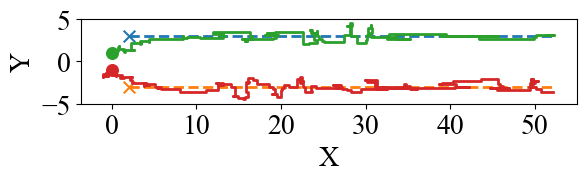
(a) $H=50$s, $T=500$ time steps ($10$Hz).

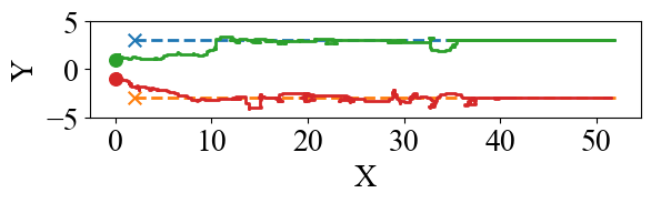
(b) $H=50$s, $T=1000$ time steps ($20$Hz).

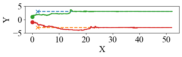
(c) $H=50$s, $T=2500$ time steps ($50$Hz).

(d) $H=50$s, $T=500$ time steps ($10$Hz).

(e) $H=50$s, $T=1000$ time steps ($20$Hz).

(f) $H=50$s, $T=2500$ time steps ($50$Hz).

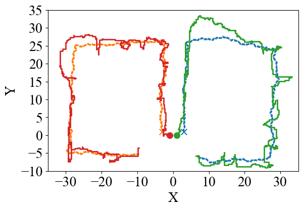
(g) $H=100$s, $T=1000$ time steps ($10$Hz).

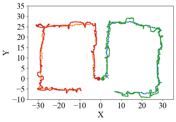
(h) $H=100$s, $T=2000$ time steps ($20$Hz).

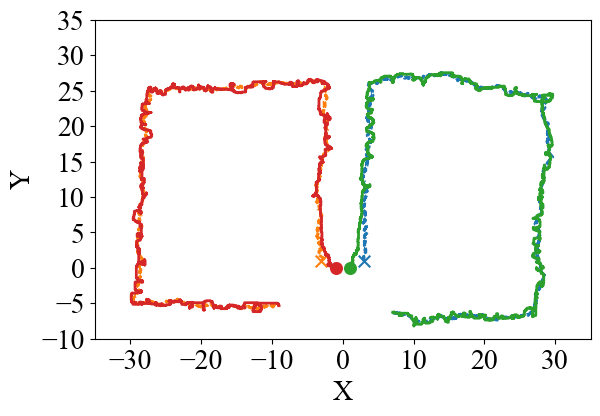
(i) $H=100$s, $T=5000$ time steps ($50$Hz).

(j) $H=100$s, $T=1000$ time steps ($10$Hz).

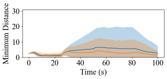
(k) $H=100$s, $T=2000$ time steps ($20$Hz).

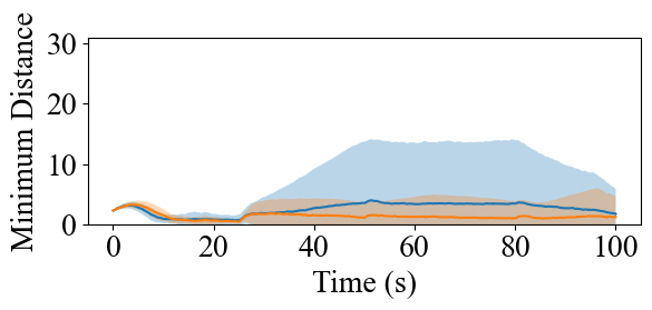
(l) $H=100$s, $T=5000$ time steps ($50$Hz).

Figure 1: Non-Adversarial Target Tracking with Multiple Robots. 2 robots pursue 2 targets that traverse trajectories that are non-adaptive to the robots motion: (a)–(c) the targets traverse the dashed straight trajectories; (g)–(i) the targets traverse the dashed noisy-rectangular trajectories that result from nominal rectangular trajectories corrupted with Gaussian noise of mean zero and variance $2$. The green and red solid lines are the robots’ trajectories, starting from the solid dots, and the blue and orange dashed lines are the targets’ trajectories, starting from the crosses. Across (a)–(c) and (g)–(i), the number $T$ of time steps per the given horizon $H$ varies, resulting in the robots to re-select actions with varying frequency. (d)–(f) and (j)–(l) depict the minimum distance from each target to a robot, averaged over 50 instances of the simulation scenarios shown in (a)–(c) and (g)–(i) respectively.

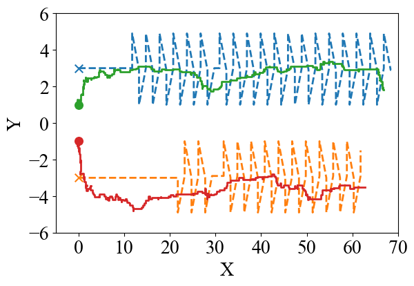
(a) Target and Robot Trajectories per OSG.

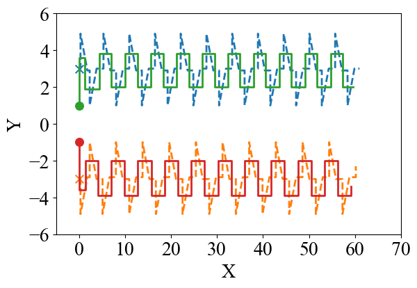
(b) Target and Robot Trajectories per ${{\sf\widehat{SG}}}$.

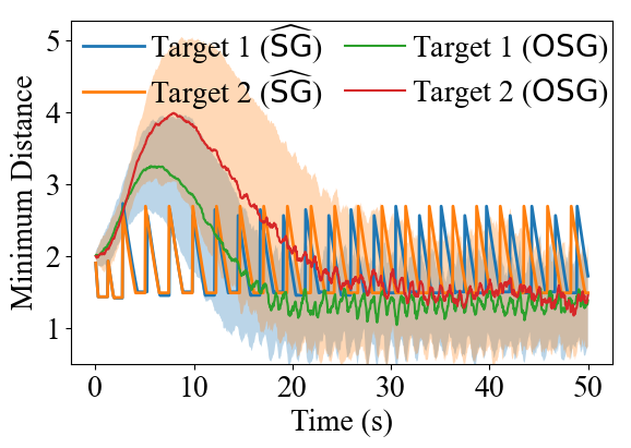
(c) Minimum Distance.

Figure 2: Adversarial Target Tracking with Multiple Robots. 2 robots pursue 2 adversarial targets over a time horizon $H=50$s. The robots re-select actions with frequency $20$Hz. The targets maneuver up or down from a nominal straight line and then forward and back to the line every time a robot is at most 1.5 units away. The robots select actions either per OSG, inducing the trajectories in (a), or per ${{\sf\widehat{SG}}}$, inducing the trajectories in (b). The green and red solid lines are the robots’ trajectories, starting from the solid dots, and the blue and orange dashed lines are the targets’ trajectories, starting from the crosses. (c) depicts the minimum distance from each target to a robot, averaged over 50 instances of scenarios (a) and (b) respectively.

We evaluate OSG in simulated scenarios of target tracking. We first consider non-adversarial targets (Section V-A), i.e., targets whose motion is non-adaptive to the robots’ motion. Then, we consider adversarial targets (Section V-B), i.e., targets whose motion adapts to the robots’ motion.

Common Simulation Setup across Simulated Scenarios. We consider two robots pursuing two targets. Particularly:

Robots

The robots can observe the exact location of the targets. The challenge is that the robots are unaware of the targets’ future motion and, as a result, the robots cannot coordinate their actions by projecting where the targets are going to be. Instead, the robots have to coordinate their actions based only on the history of past observations and somehow guess the future. To move in the environment, each robot $i\in{\cal N}$ can perform either of the actions {“upward”, “downward”, “left”, “right”} at a speed of {$1$, $2$} units/s.

Targets

The targets are either non-adversarial or adversarial, moving on the same 2D plane as the robots. The available actions to the targets in each of the two scenarios are described in Section V-A and Section V-B, respectively.

Objective Function

The robots coordinate their actions $\{a_{i,\,t}\}_{i\,\in\,{\cal N}}$ to maximize at each time step $t$

$${f_{t}(\,\{a_{i,\,t}\}_{i\,\in\,{\cal N}}\,)\,=\,\sum_{j\,\in\,{\cal T}}\;\max_{i\,\in\,{\cal N}}\;\frac{1}{d_{t}(a_{i,\,t},\,j)},}$$ (10)

where $d_{t}(a_{i,\,t},\,j)$ is the distance between robot $i$ and target $j$ after $a_{i,\,t}$ has been executed. Hence, $d_{t}(a_{i,\,t},\,j)$ is known to the robots only once the robots have executed their actions and the targets’ locations at time step $t$ have been observed.

By maximizing $f_{t}$, the robots aim to “capture” the targets: $f_{t}$ indicates that if robot $i$ keeps being the closest to target $j$, then the remaining robots receive no marginal gain by trying to approach target $j$ and thus they would want to approach other targets to maximize the objective.

Computer System Specifications. We performed all simulations in Python 3.9.7, on a MacBook Pro equipped with the Apple M1 Max chip and a 32 GB RAM.

Code. Our code is available at: https://gitlab.umich.edu/iral-code/ral23-online-submodular-coordination.

V-A Non-Adversarial Targets: Non-Adaptive Target Trajectories

Simulation Setup. We consider two scenarios of non-adaptive target trajectories: (i) the targets traverse predefined straight lines over a time horizon $H=50$s with speed $1$ unit/s (Fig. 1(a-c)), and (ii) the targets traverse noisy rectangular-like trajectories over a time horizon $H=100$s (Fig. 1(g-i)); specifically, the rectangular-like trajectories are generated by targets that follow a nominal rectangular trajectory with speed $1$ unit/s while randomizing their lateral speed by sampling from a Gaussian distribution with zero mean and variance $2$. For each case, we evaluate OSG when the robots’ action re-selection frequency varies from $10$Hz to $20$Hz to $50$Hz.

Results. The simulation results are presented in Fig. 1. They reflect the theoretical analyses in Section IV-B. At $10$Hz, the robots fail to “learn” the targets’ future motion, failing to reduce their distance to them (Fig. 1(a,d,g,j)). The situation improves at $20$Hz (Fig. 1(b,e,h,k)), and even further at $50$Hz (Fig. 1(c,f,i,l)), in which case the robots closely track the targets. The average minimum distances improve from $2$ ($10$Hz) to $1$ ($20$Hz) to $0.3$ ($50$Hz) unit for the line case (Fig. 1(d-f)), and from $8$ ($10$Hz) to $4$ ($20$Hz) to $2$ ($50$Hz) units for the noisy-rectangular case (Fig. 1(j-l)).

V-B Adversarial Targets: Adaptive Target Trajectories

Simulation Setup. We consider targets that maneuver when the robots are close enough. As long as the robots are more than $1.5$ units away from a target $j$, the target $j$ will keep moving “right” on a nominal straight line at a speed $1$ unit/s. But once a robot is within $1.5$ units away, then target $j$ will perform a maneuver: target $j$ will first choose from moving “upward” or “downward” at $2$ units/s for $1$s to maximize the distance from the robots, and then will move diagonally for $0.05$s to return back to the nominal path with vertical speed $40$ units/s and horizontal speed to the “right” $30$ units/s.

To demonstrate the need for randomization in adversarial environments (Remark 3), we compare OSG with a deterministic algorithm that selects actions at each $t$ with respect to the previously observed $f_{t-1}$. We denote the algorithm by ${{\sf\widehat{SG}}}$ since it is a (heuristic) extension of the Sequential Greedy algorithm [13] to 1’s setting per the rule:

$$a_{i,\,t}^{{{{\sf\widehat{SG}}}}}\,\in\,\max_{a\,\in\,{\cal V}_{i}}\;f_{t-1}(\,a\;|\;\{a_{1,\,t}^{{{\sf\widehat{SG}}}},\ldots,a_{i-1,\,t}^{{{\sf\widehat{SG}}}}\}\,).$$ (11)

The Sequential Greedy algorithm [13] instead selects actions per the rule in eq. 5, given the a priori knowledge of $f_{t}$.

Results. The simulation results are presented in Fig. 2. OSG performs better than ${{\sf\widehat{SG}}}$, as expected since ${{\sf\widehat{SG}}}$ prescribes actions to the robots “blindly” by deterministically following the target’s previous position, instead of accounting for the whole history of the targets’ past motions as OSG does: OSG triggers $50\%$ more target maneuvers than ${{\sf\widehat{SG}}}$ ($31$ maneuvers in Fig. 2(a) vs. $20$ maneuvers in Fig. 2(b)), implying OSG tracks the targets closer than ${{\sf\widehat{SG}}}$; particularly, once OSG has “learned” the target’s future motion (after the $30$-th second in Fig. 2(c)), OSG results in average minimum distances to each target that are $20$% smaller than ${{\sf\widehat{SG}}}$’s.

VI Conclusion

Summary. We introduced the first algorithm for efficient and effective online submodular coordination in unpredictable environments (OSG): OSG is the first polynomial-time algorithm with bounded tracking regret for 1. The bound gracefully degrades with the environments’ capacity to change adversarially, quantifying how frequently the agents must re-select actions to “learn” to coordinate as if they knew the future a priori. OSG generalizes the seminal Sequential Greedy algorithm [13] to 1’s online optimization setting. To this end, we leveraged the FSF^⋆ algorithm for the problem of tracking the best expert. We validated OSG in simulated scenarios of target tracking.

Future Work. We plan for the future work:

Partial Information Feedback

OSG selects actions at each $t$ based on full information feedback, i.e., based on the availability of the functions $f_{k}:2^{{\cal V}_{\cal N}}\mapsto\mathbb{R}$ for each $k\leq t-1$. The availability of these functions relies on the assumption that the agents can simulate the environment from the beginning of each step $k$ till its end. But the agents may lack the resources for this. We will enable OSG to rely only on partial information, i.e., only on the observed values $f_{k}(\,\{a_{i,\,k}\}_{i\,\in\,{\cal N}}^{\sf OSG}\,)$ per the executed actions $\{a_{i,\,k}^{\sf OSG}\}_{i\,\in\,{\cal N}}$.

Best of Both Worlds (BoBW)

OSG selects actions assuming the environment may evolve arbitrarily in the future. The assumption is pessimistic when the environment’s evolution is governed by a stochastic (yet unknown) model. For example, OSG’s performance against the non-adversarial targets in Section V-A, although it becomes near-optimal for large $T$, is pessimistic: the deterministic heuristic ${{\sf\widehat{SG}}}$ can be shown to perform better since by construction $f_{t-1}\simeq f_{t}$ in Section V-A. We will extend OSG such that it offers BoBW suboptimality guarantees [37]. BoBW guarantees become especially relevant under partial information feedback since then heuristics such as the ${{\sf\widehat{SG}}}$ cannot apply in the first place.

Appendix

-A Proof of Theorem 1

We use the notation:

• ${\cal A}^{{\sf OPT}}_{i-1,\,t}$ is the optimal solution set for the first $i-1$ agents at time step $t$;

• $\Delta_{i}(T)\triangleq\sum_{t=1}^{T-1}{\bf 1}(a_{i,\,t}^{\sf OPT}\neq a_{i,\;t+1}^{\sf OPT})$ is the change of environment for agent $i$, i.e., $\sum_{i\,\in\,\mathcal{N}}\Delta_{i}(T)=\Delta(T)$.

We have:

$$\sum_{t=1}^{T}f_{t}(\,{\cal A}^{{\sf OPT}}_{t}\,)\leq\sum_{t=1}^{T}f_{t}(\,{\cal A}^{{\sf OPT}}_{t}\cup{\cal A}^{{\sf OSG}}_{t}\,)$$ (12)

$$=\sum_{t=1}^{T}f_{t}(\,{\cal A}^{{\sf OSG}}_{t}\,)+\sum_{t=1}^{T}\sum_{i\,\in\,{\cal N}}f_{t}(a_{i,\,t}^{\sf OPT}\,|\,{\cal A}^{{\sf OPT}}_{i-1,\,t}\cup{\cal A}^{{\sf OSG}}_{t}\,)$$ (13)

$$\leq\sum_{t=1}^{T}f_{t}(\,{\cal A}^{{\sf OSG}}_{t}\,)+\sum_{t=1}^{T}\sum_{i\,\in\,{\cal N}}f_{t}(a_{i,\,t}^{\sf OPT}\,|\,{\cal A}^{{\sf OSG}}_{i-1,\,t}\,)$$ (14)

$$=2\sum_{t=1}^{T}f_{t}(\,{\cal A}^{{\sf OSG}}_{t}\,)$$

$$\quad+\sum_{t=1}^{T}\sum_{i\,\in\,{\cal N}}f_{t}(a_{i,\,t}^{\sf OPT}\,|\,{\cal A}^{{\sf OSG}}_{i-1,\,t}\,)-f_{t}(a_{i,\,t}^{\sf OSG}\,|\,{\cal A}^{{\sf OSG}}_{i-1,\,t}\,)$$ (15)

$$=2\sum_{t=1}^{T}f_{t}(\,{\cal A}^{{\sf OSG}}_{t}\,)+\sum_{t=1}^{T}\sum_{i\,\in\,{\cal N}}r_{a^{\sf OPT},\,t}^{\hskip 0.5pt(i)}-r_{a^{\sf OSG},\,t}^{\hskip 0.5pt(i)},$$ (16)

where eq. 12 holds from the monotonicity of $f_{t}$; eqs. 13 and 15 are proved by telescoping the sums; eq. 14 holds from the submodularity of $f_{t}$; and eq. 16 holds from the definition of $r_{a,\,t}^{\hskip 0.5pt(i)}$ (OSG’s line 14). We now complete the proof:

$$\mathbb{E}\Bigl{[}{{\sf Tracking}\text{-}{\sf Regret}_{T}^{(1/2)}}(\,{\cal A}^{{\sf OSG}}\,)\Bigr{]}$$

$$=\mathbb{E}\Bigl{[}\frac{1}{2}\sum_{t=1}^{T}f_{t}(\,{\cal A}^{{\sf OPT}}_{t}\,)-\sum_{t=1}^{T}f_{t}(\,{\cal A}^{{\sf OSG}}_{t}\,)\Bigr{]}$$ (17)

$$\leq\frac{1}{2}\sum_{t=1}^{T}\sum_{i\,\in\,{\cal N}}\mathbb{E}\Big{[}r_{a^{\sf OPT},\,t}^{\hskip 0.5pt(i)}-r_{a^{\sf OSG},\,t}^{\hskip 0.5pt(i)}\Big{]}$$ (18)

$$=\frac{1}{2}\sum_{t=1}^{T}\sum_{i\,\in\,{\cal N}}r_{a^{\sf OPT},\,t}^{\hskip 0.5pt(i)}-r_{t}^{\hskip 0.5pt(i)\top}p_{t}^{(i)}$$ (19)

$$\leq\frac{1}{2}\times 8\sum_{i\,\in\,{\cal N}}\sqrt{T\Big{(}(\Delta_{i}(T)+1)\log{(|{\cal V}_{i}|T)}+l\Big{)}}$$ (20)

$$\leq 4\sqrt{|{\cal N}|T\sum_{i\,\in\,{\cal N}}\Big{(}(\Delta_{i}(T)+1)\log{(|{\cal V}_{i}|T)}+l\Big{)}}$$ (21)

$$\leq 4\sqrt{|{\cal N}|T\Big{(}(\Delta(T)+|{\cal N}|)\log{(\max_{i\,\in\,{\cal N}}{|{\cal V}_{i}|}T)}+|{\cal N}|l\Big{)}},$$ (22)

where $l\triangleq\log{(1+\log{(T)})}$, eq. 17 holds from Definition 2; eq. 18 holds from eq. 16; eq. 19 holds from the internal randomness of FSF${}^{\star}|_{i}$; eq. 20 holds from [33, Corollary 1]; eq. 21 holds from the Cauchy–Schwarz inequality; and eq. 22 holds since $\sum_{i\,\in\,{\cal N}}\Delta_{i}(T)=\Delta(T)$. ∎

-B Proof of Monotonicity and Submodularity of Function (10)

It suffices to prove that $\max\colon 2^{\mathbb{R}}\mapsto\mathbb{R}$ is non-decreasing and submodular. Indeed, if ${\cal A}\subseteq{\cal B}\in 2^{\mathbb{R}}$, then $\max({\cal A})\leq\max({\cal B})$, i.e., $\max$ is non-decreasing. Next, consider finite and disjoint ${\cal B}_{1}\in 2^{\mathbb{R}}$ and ${\cal B}_{2}\in 2^{\mathbb{R}}$, and an arbitrary real number $s$. Then, using Table I we verify that $\max(s\,|\,{\cal B}_{1})$ $\geq\max{(s\,|\,{\cal B}_{1}\cup{\cal B}_{2})}$ holds true, i.e., $\max$ is submodular. ∎

	$\max{(s\,|\,{\cal B}_{1})}$	$\max{(s\,|\,{\cal B}_{1}\cup{\cal B}_{2})}$
$s\leq\min{(b_{1},b_{2})}$	0	0
$b_{1}<s<b_{2}$	$s-b_{1}$	0
$b_{2}<s<b_{1}$	0	0
$\max{(b_{1},b_{2})}\leq s$	$s-b_{1}$	$s-\max{(b_{1},b_{2})}$
$b_{1}=b_{2}$	$\max{(0,s-b_{1})}$	$\max{(0,s-b_{1})}$

TABLE I: Comparison of $\max{(s\,|\,{\cal B}_{1})}$ and $\max{(s\,|\,{\cal B}_{1}\cup{\cal B}_{2})}$ for all relationships of $b_{1}$, $b_{2}$, and $s$, where $b_{1}\triangleq\max{({\cal B}_{1})}$ and $b_{2}\triangleq\max{({\cal B}_{2})}$.

References

- [1] M. Corah and N. Michael, “Scalable distributed planning for multi-robot, multi-target tracking,” in IEEE/RSJ International Conference on Intelligent Robots and Systems (IROS), 2021, pp. 437–444.
- [2] N. Atanasov, J. Le Ny, K. Daniilidis, and G. J. Pappas, “Decentralized active information acquisition: Theory and application to multi-robot SLAM,” in IEEE International Conference on Robotics and Automation (ICRA), 2015, pp. 4775–4782.
- [3] B. Schlotfeldt, V. Tzoumas, and G. J. Pappas, “Resilient active information acquisition with teams of robots,” IEEE Transactions on Robotics (TRO), vol. 38, no. 1, pp. 244–261, 2021.
- [4] A. Krause, A. Singh, and C. Guestrin, “Near-optimal sensor placements in gaussian processes: Theory, efficient algorithms and empirical studies,” Jour. of Mach. Learn. Res. (JMLR), vol. 9, pp. 235–284, 2008.
- [5] A. Singh, A. Krause, C. Guestrin, and W. J. Kaiser, “Efficient informative sensing using multiple robots,” Journal of Artificial Intelligence Research, vol. 34, pp. 707–755, 2009.
- [6] P. Tokekar, V. Isler, and A. Franchi, “Multi-target visual tracking with aerial robots,” in IEEE/RSJ International Conference on Intelligent Robots and Systems (IROS), 2014, pp. 3067–3072.
- [7] B. Gharesifard and S. L. Smith, “Distributed submodular maximization with limited information,” IEEE Transactions on Control of Network Systems (TCNS), vol. 5, no. 4, pp. 1635–1645, 2017.
- [8] D. Grimsman, M. S. Ali, J. P. Hespanha, and J. R. Marden, “The impact of information in distributed submodular maximization,” IEEE Trans. on Contr of Netw. Sys. (TCNS), vol. 6, no. 4, pp. 1334–1343, 2018.
- [9] M. Corah and N. Michael, “Distributed submodular maximization on partition matroids for planning on large sensor networks,” in IEEE Conference on Decision and Control (CDC), 2018, pp. 6792–6799.
- [10] ——, “Distributed matroid-constrained submodular maximization for multi-robot exploration: Theory and practice,” Autonomous Robots (AURO), vol. 43, no. 2, pp. 485–501, 2019.
- [11] L. Zhou, V. Tzoumas, G. J. Pappas, and P. Tokekar, “Resilient active target tracking with multiple robots,” IEEE Robotics and Automation Letters (RAL), vol. 4, no. 1, pp. 129–136, 2018.
- [12] U. Feige, “A threshold of for approximating set cover,” Journal of the ACM (JACM), vol. 45, no. 4, pp. 634–652, 1998.
- [13] M. L. Fisher, G. L. Nemhauser, and L. A. Wolsey, “An analysis of approximations for maximizing submodular set functions–II,” in Polyhedral combinatorics, 1978, pp. 73–87.
- [14] M. Sun, M. E. Davies, I. Proudler, and J. R. Hopgood, “A gaussian process based method for multiple model tracking,” in Sensor Signal Processing for Defence Conference (SSPD), 2020, pp. 1–5.
- [15] N. Cesa-Bianchi and G. Lugosi, Prediction, Learning, and Games. Cambridge university press, 2006.
- [16] J. Liu, L. Zhou, P. Tokekar, and R. K. Williams, “Distributed resilient submodular action selection in adversarial environments,” IEEE Robotics and Automation Letters (RAL), vol. 6, no. 3, pp. 5832–5839, 2021.
- [17] A. Robey, A. Adibi, B. Schlotfeldt, H. Hassani, and G. J. Pappas, “Optimal algorithms for submodular maximization with distributed constraints,” in Learn. for Dyn. & Cont. (L4DC), 2021, pp. 150–162.
- [18] N. Rezazadeh and S. S. Kia, “Distributed strategy selection: A submodular set function maximization approach,” arXiv:2107.14371, 2021.
- [19] R. Konda, D. Grimsman, and J. R. Marden, “Execution order matters in greedy algorithms with limited information,” in American Control Conference (ACC), 2022, pp. 1305–1310.
- [20] Z. Xu and V. Tzoumas, “Resource-aware distributed submodular maximization: A paradigm for multi-robot decision-making,” in IEEE Conference on Decision and Control (CDC), 2022, pp. 5959–5966.
- [21] M. Streeter and D. Golovin, “An online algorithm for maximizing submodular functions,” Advances in Neural Information Processing Systems (NeurIPS), vol. 21, 2008.
- [22] M. Streeter, D. Golovin, and A. Krause, “Online learning of assignments,” Advances in Neu. Inform. Proc. Sys. (NeurIPS), vol. 22, 2009.
- [23] D. Suehiro, K. Hatano, S. Kijima, E. Takimoto, and K. Nagano, “Online prediction under submodular constraints,” in International Conference on Algorithmic Learning Theory (ALT), 2012, pp. 260–274.
- [24] D. Golovin, A. Krause, and M. Streeter, “Online submodular maximization under a matroid constraint with application to learning assignments,” arXiv preprint:1407.1082, 2014.
- [25] L. Chen, H. Hassani, and A. Karbasi, “Online continuous submodular maximization,” in International Conference on Artificial Intelligence and Statistics (AISTATS). PMLR, 2018, pp. 1896–1905.
- [26] M. Zhang, L. Chen, H. Hassani, and A. Karbasi, “Online continuous submodular maximization: From full-information to bandit feedback,” Adv. in Neu. Inform. Proc. Sys. (NeurIPS), vol. 32, 2019.
- [27] M. Herbster and M. K. Warmuth, “Tracking the best expert,” Machine learning, vol. 32, no. 2, pp. 151–178, 1998.
- [28] A. György, T. Linder, and G. Lugosi, “Tracking the best of many experts,” in International Conference on Computational Learning Theory (COLT). Springer, 2005, pp. 204–216.
- [29] A. György, T. Linder, G. Lugosi, and G. Ottucsák, “The on-line shortest path problem under partial monitoring.” Journal of Machine Learning Research (JMLR), vol. 8, no. 10, 2007.
- [30] L. Zhang, T. Yang, J. Yi, R. Jin, and Z.-H. Zhou, “Improved dynamic regret for non-degenerate functions,” Adv. in Neu. Inform. Proc. Sys. (NeurIPS), vol. 30, 2017.
- [31] L. Zhang, S. Lu, and Z.-H. Zhou, “Adaptive online learning in dynamic environments,” Adv. in Neu. Inform. Proc. Sys. (NeurIPS), vol. 31, 2018.
- [32] N. Harvey, C. Liaw, and T. Soma, “Improved algorithms for online submodular maximization via first-order regret bounds,” Adv. in Neu. Inform. Proc. Sys. (NeurIPS), vol. 33, pp. 123–133, 2020.
- [33] T. Matsuoka, S. Ito, and N. Ohsaka, “Tracking regret bounds for online submodular optimization,” in International Conference on Artificial Intelligence and Statistics (AISTATS). PMLR, 2021, pp. 3421–3429.
- [34] A. Downie, B. Gharesifard, and S. L. Smith, “Submodular maximization with limited function access,” IEEE Tran. on Auto. Cont. (TAC), 2022.
- [35] J. Robinson and M. Herbster, “Improved regret bounds for tracking experts with memory,” Advances in Neural Information Processing Systems (NeurIPS), vol. 34, pp. 7625–7636, 2021.
- [36] M. Sviridenko, J. Vondrák, and J. Ward, “Optimal approximation for submodular and supermodular optimization with bounded curvature,” Math. of Operations Research, vol. 42, no. 4, pp. 1197–1218, 2017.
- [37] S. Ito, “On optimal robustness to adversarial corruption in online decision problems,” Advances in Neural Information Processing Systems (NeurIPS), vol. 34, pp. 7409–7420, 2021.