NNPred: A Predictor Library to Deploy Neural Networks in Computational Fluid Dynamics software

Abstract

A neural-networks predictor library has been developed to deploy machine learning (ML) models into computational fluid dynamics (CFD) codes. The pointer-to-implementation strategy is adopted to isolate the implementation details in order to simplify the implementation to CFD solvers. The library provides simplified model-managing functions by encapsulating the TensorFlow C library, and it maintains self-belonging data containers to deal with data type casting and memory layouts in the input/output (I/O) functions interfacing with CFD solvers. On the language level, the library provides application programming interfaces (APIs) for C++ and Fortran, the two commonly used programming languages in the CFD community. High-level customized modules are developed for two open-source CFD codes, OpenFOAM and CFL3D, written with C++ and Fortran, respectively. The basic usage of the predictor is demonstrated in a simple data-driven heat transfer problem as the first tutorial case. Another tutorial case of modeling the effect of turbulence in channel flow using the library is implemented in both OpenFOAM and CFL3D codes. The developed ML predictor library provides a powerful tool for the deployment of ML models in CFD solvers.

PROGRAM SUMMARY

Program Title: NNPred
CPC Library link to program files: (to be added by Technical Editor)
Developer’s respository link: https://github.com/Weishuo93/NN_Pred
Code Ocean capsule: (to be added by Technical Editor)
Licensing provisions: MIT, LGPL, Apache-2.0
Programming language: C/C++, Fortran
Nature of problem:
Coupling machine learning models with CFD programs with minimal modifications in CFD codes.
Solution method:
Adopting pointer-to-implementation (Pimpl) strategy to isolate the implementation details and developing different levels of API and modules on programming language and CFD solvers respectively.
Additional comments including restrictions and unusual features :
Currently rely on TensorFlow as the machine learning model’s backends.

1 Introduction

In recent years, the machine learning (ML) technology has been empowering the development of computational fluid dynamics (CFD) in many aspects, with specific applications in turbulence modeling [1, 2], reduced order modeling [3, 4, 5], uncertainty quantification [6, 7, 8, 9], flow control [10, 11], grid generation [12, 13, 14], and etc. ML technology owns its advantage of extracting complex mapping relations from collected data, therefore can speed up the empirical modeling process that would otherwise require a significant amount of human experience. More significantly, such ML-integrated applications generally have superior performance against empirical methods especially for complex systems (e.g., turbulence). Numerous elaborate revisions have demonstrated the feasibility of integrating ML techniques in a CFD toolset [15, 16], indicating their huge potential in both academic and industrial scenarios.

However, there exists a noticeable barrier in terms of the programming infrastructures between typical ML workflow and conventional CFD solvers, since the mainstream programming languages are fundamentally different between the two communities. For training the ML models, interpretive languages (e.g., Python) are generally adopted for their convenience in run-time execution and searching for optimal configuration of the model [17, 18, 19, 20]. But for CFD solvers, compiled languages such as C/C++ and Fortran are widely used for the efficiency of massive floating-point operations [21, 22, 23, 24]. Researchers or engineers might need to spend a great amount of time and effort implementing and testing an ML model within a CFD solver.

From the technical perspective, deploying a trained ML model to an application program can take the following options. The first option is to drive the Python interpreter [25] inside the CFD program. But at each iteration step, the in-memory data needs to be packed as Python objects and passed to the model prediction function written in Python, and vice versa for the returned Python arrays [26, 27]. The implementation can be highly customized, but the massive converting process would cause a significant overhead of computer resources, making it only suitable for some small-scale calculations. Another method is to reconstruct the ML model with the CFD’s native language according to the model’s information saved from Python scripts. This strategy could maintain good compatibility with the CFD program, and has been adopted by the Fortran-Keras Bridge library [28]. However, active development is needed to keep up with the updates of ML libraries, which are currently fast-changing, and if one were to reconstruct a complex NN architecture in CFD software, some new features from the updated ML library might be not available timely. However, most wide-used ML frameworks (e.g., TensorFlow and PyTorch) provide binary libraries with native binding application programming interfaces (APIs) in fundamental languages (e.g., C/C++), which might be compatible with CFD codes. Their computational efficiency is normally optimized internally, and the newest features are naturally updated. Therefore, utilizing the ML libraries’ binding APIs became the best choice to take into account the computational efficiency, complex model structures, and coding compatibility. For example, Geneva and Zabaras deployed a neural network (NN) from PyTorch [19] into OpenFOAM [21] for uncertainty quantification studies [9]. Maulik et al. [29] employed the TensorFlow (TF) C-API [30] also in OpenFOAM and formulate Reynolds-Averaged Navier–Stokes (RANS) and large eddy simulation (LES) solvers calling runtime ML predictions. Shin et al. modeled subgrid-scale closure in OpenFOAM LES solver via OpenVINO [31], which is an artificial intelligence (AI) inference toolkit designed for Intel CPU.

Nonetheless, the deployment of ML models still remains a challenge for CFD programmers. It may take developers a lot of effort to find the APIs to call a model’s forward prediction. Besides, since ML models are normally trained on GPU but CFD codes are mainly applied on CPU clusters, problems might exist in data type casting and parallelization. To deal with the above-mentioned difficulties, we develop a neural-networks (NN) predictor library under the pointer-to-implementation (Pimpl) strategy [32, 33], which isolates the implementation detail so that its implementation to CFD software can be largely simplified. The library provides simplified model-managing functions by encapsulating the TensorFlow C-API, and maintains self-belonging data containers to automatically deal with data type casting and memory layouts in the I/O functions interfacing with CFD solvers. The process of the implementation is simplified to two major steps: initialization and prediction, where each step can be achieved using only 3-4 lines of scripts. The library currently supports APIs for two languages: C++ and Fortran, with high-level customized modules for two open-source CFD codes, OpenFOAM (OF) and CFL3D [22]. The former is written in C++, following the object-oriented programming (OOP) paradigm, whereas the latter is NASA’s compressible CFD solver written in Fortran, and has been widely applied in many projects [34] since the 1980s.

In this paper, two tutorial cases are presented to demonstrate the usage of the library. First, a heat transfer problem is considered to introduce the basic process to call the ML model’s prediction from a general partial differential equation solver. The Laplacian solver of the OpenFOAM is modified for this application. In the second tutorial case, the methodology of the iterative ML-RANS framework of Liu et al. [35, 36] is reproduced in both OpenFOAM and CFL3D. The effect of turbulence in a channel flow is modeled by NN in this case. The computational efficiency and parallel performance are also tested for both codes. By maintaining an independent predictor in each thread to perform serial local predictions, the CFD program’s original message passing interface (MPI) pattern [37] does not need to be re-designed, and no extra message passing load is increased. The source code repository is publicly available and free of use.

The paper is organized as follows. Section 2 describes the program design of the library, including its basic application workflow, API hierarchy, and a minimal example explaining the runtime model controlling and data I/O mechanism. In Sec. 3, the tutorial cases, i.e., the heat transfer and turbulent channel flow, are presented. Conclusions are drawn in the last section (Sec. 4).

2 Library Design

In this section, the program design of the predictor library is introduced. First, the library’s typical application workflow with its fundamental structure is shown in subsection. 2.1 to provide an initial intuitive understanding of where and how this library should be used. Then the Pimpl concept is introduced to develop a well-isolated pure-method class, based on which the API hierarchy in Fortran and higher-level CFD programs are established (subsection. 2.2). Finally, the predictor’s model loading and runtime data I/O mechanisms are demonstrated by running a simple A + B model with a minimal C++ code example (subsection. 2.3). This example is also used in the API manual, documented in B, to facilitate understanding the API usage in different languages and CFD programs.

2.1 Library Structure and Basic Workflow

The typical workflow and the library structure are shown in Fig. 1. The core functionality of this library includes, loading a trained model, performing prediction, and I/O with external data sources. Structurally, this library has two main parts. The first part is the model-control methods, which wraps the TensorFlow C library [30] to impose controls on the model’s initialization and prediction. The control methods significantly simplify the calling process, thus reducing the difficulty in deploying the ML model. The other is the data methods with self-maintained data containers and the I/O functions from/to external data sources. Normally, the external sources might be from another programming language (e.g., Fortran in many legacy codes) or under a specific data structure (e.g., the volScalarField in OpenFOAM), therefore, customized I/O function with data type and memory layout changing options are provided for adaption to CFD codes.

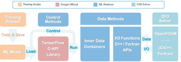
Figure 1: The structure and work flow of the ML predictor library.

The predictor library is designed with the following features to facilitate the deployment of a ML model:

• Supported format.:

  • PB graph (normally saved by TensorFlow version 1 scripts)

  • SavedModel (normally saved by Keras APIs)

• Parallelization:

  • Automatic parallelization on idle CPUs (default setting for TensorFlow C library)

  • Manually set core numbers for model prediction to adapt a parallel computation

• Data I/O:

  • Automatic data type casting according to the external source/target arrays

  • Memory layout changing options (adaption of row/column-major layout)

2.2 The Pimpl Paradigm and API hierarchy

The top-level design of this predictor library follows the Pimpl paradigm. It is an implementation-hiding technique in which a public class wraps a structure or class that cannot be seen outside the library [33]. In the predictor library, control methods, data methods, and the inner data container are all well-isolated, and the exposed public class is designed as a pure method class. This wrapping style reconciles the possibility of implementing the library in both object-oriented and process-oriented programs. The API hierarchy is shown in Fig. 2, where the core predictor class is written with C++ under the Pimpl paradigm. The Fortran APIs are then developed via the ISO_C_BINDING module [38, 39] from the C++ core predictor. The language-level APIs are then further encapsulated into program-level modules for OpenFOAM and CFL3D, which could read settings from text setup files. In this way, the model deployment is further simplified and the modification of CFD codes could be minimized.

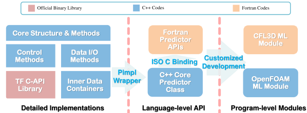
Figure 2: The API hierarchy relationships of the predictor library.

The Pimpl strategy is achieved in C++ with the d-pointer technique [40], which means the public class only needs to maintain a private pointer to the implementation class. The detailed methods and data are actually coded in the implementation class. A demonstrative bare-bone header for the public class is shown in Listing 1, where the implementation class only needs to be declared (line 2) without any further definition, and the public class can utilize the private implementation-class pointer (defined in line 20) to realize all the public methods.

⬇

1// Declaration of the Impl class

2class PredictorImpl;

3

4// The public class exposed to users

5class Predictor {

6

7 public:

8 // Constructors:

9 explicit Predictor(std::string pbfile);

10 // ... ... Other constructors will be introduced in the API section.

11

12 // Destructor:

13 virtual ~Predictor();

14

15 // Class methods: initialization, data I/O, model running functions ...

16 // ... ... ... will be introduced in detail in the API section.

17

18 private:

19 // d-pointer to hide implementation details from the users

20 PredictorImpl *d;

21

22};

Listing 1: Main structure of the predictor library’s header

2.3 Minimal example with A+B Model

We use a simple A + B model to illustrate the basic process of deploying an ML model in C++ code, which includes initializing the model, performing prediction, and interfacing with outer memory spaces. This minimal example can be seen as an entry-level getting-started tutorial, and the entire detailed API documentation is also demonstrated with this example, which is documented in B. The installation guide with the necessary dependencies and compile options can be found in A.

2.3.1 Explanation of the A + B model and its saved formats

Basically, the predictor library adopts TensorFlow C library [30] to manage models, and therefore, any TensorFlow supported formats are accepted in the present library. At the fundamental level, TensorFlow defines an ML model as sequential records of how data is manipulated mathematically till the outputs are obtained. Each mathematical operation or the input/output data placeholder is recorded as a node, and a series of nodes in a collection constitutes a graph. At higher levels, TensorFlow integrates Keras [41] to compose models. Keras provides frequently used NN layer APIs by grouping basic node operations, and the model management methods (e.g., training, evaluation, prediction, and saving) are also well encapsulated. The high-level model (i.e., created by Keras) is normally saved in the official SavedModel format.

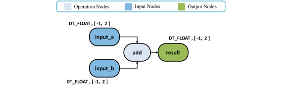
Figure 3: The API hierarchy relationships of the predictor library.

The A + B model is simply to get the summation of two arrays, in which the operation of adding two 2D arrays (i.e., A and B) is recorded. The A + B model has two input arrays with dimension size: $n$ $\times$ 2, where n is the number of data instances. The shape of the output is also an $n$ $\times$ 2 array, holding the summation of the two input arrays. The node definitions are shown in Fig. 3, with the data type being specified as the single precision floating point (DT_FLOAT under TensorFlow’s definition). The model can be created in two different ways and stored in the corresponding formats. One way acts bottom-to-top to establish graphs from basic operations, such graphs are saved in protocol buffers (PB) format [42] (with file extensions *.pb) as a sequential stream of bytes. While the other way uses Keras to build and saves the models in the SavedModel format (which is actually a folder). The two methods for building and saving ML models can be viewed in the Python script: createmodel_AplusB.py in the repository. The command-line usage to create the two different formats is shown in  B.

Note that the library is upward compatible with TensorFlow. The higher version of TensorFlow can load the model from the library using a lower version of TensorFlow, but the reverse operation would raise an incompatibility problem. The model saved in a TensorFlow version 2 Keras SavedModel format can not be loaded via a TensorFlow version 1 binary library.

2.3.2 Runtime model control and data I/O via C++ example

In this part, the A + B model is loaded in a C++ code example to demonstrate the runtime model control and data I/O mechanism of the predictor. The PB graph format, simple_graph_tf2.pb, is used in the code snippet example, and the alternative APIs for other TensorFlow format is introduced in the documentation (B).

Table 1: Lines of scripts required for each step of the program

Initialization		Prediction
Program Step	Lines of scripts *	Program Step	Lines of Codes *
Load Model	1	Set Input Data	$\boldsymbol{N}_{i}$
Register Nodes	$\boldsymbol{N}_{io}$	Run Model	1
Set Data Number	1	Get Output Data	$\boldsymbol{N}_{o}$

• $\boldsymbol{N}_{i}$, $\boldsymbol{N}_{o}$, and $\boldsymbol{N}_{io}$ stands for the number of input nodes, output nodes and their summation.

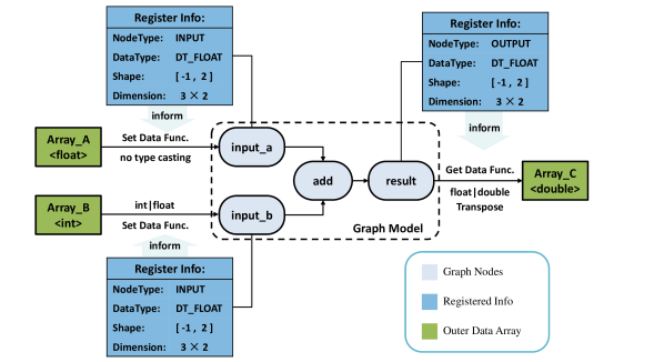
Figure 4: Interaction relation within predictor elements and with outer memory spaces during a prediction process.

Basically, the overall process can be divided into two major parts: initialization and prediction. Each part can be implemented with several lines of scripts (see Table 1). The initialization part consists of loading the model, registering the input/output nodes, and setting the number of data instances, whereas the prediction part includes setting the input data, running predictions, and extracting the result.

Figure 4 illustrates how the different elements in the predictor interact with others, and an example of the scripts is shown in Listing 2. The loading procedure is achieved by creating the predictor object with the model’s path being specified (line 7 in the code example), in which, all the definitions of nodes are cached (circled by the dotted line in Fig. 4). Then users should register nodes by specifying the nodes’ name and input/output type (line 11-16 in Listing 2). In this process, the pieces of information of the registered nodes are extracted and recorded for the automatic I/O functions (blue tables in Fig.4). Finally, the initialization process can be considered completed after setting the number of data instances (line 19 in Listing 2), after which the predictor will allocate memory space for the inner data containers according to the recorded data types and dimensions.

Afterward, three C++ arrays are created (line 21-26 in Listing 2) to represent the external sources of data. In the prediction process, the input data is first mapped to the predictor’s input container through the set data function (line 28-30 in Listing 2). Then the model is executed (line 33 in Listing 2) and the output containers are filled with computation results, which will finally be extracted to the external arrays via the get-data function (line 36 in Listing 2). It needs to be mentioned that the data type of the external arrays is not necessarily consistent with the model-defined type (e.g., float). The set/get data function can automatically cast the data according to the recorded node information (done by the register function) to ensure a correct computational result. For example, the set-data function casts the integers from Array_B to floats as defined by the node container input_b. Apart from this, the external array’s memory layout can also be specified during the I/O process. Fig. 5 shows the process to extract the output data into a column-majored memory space.

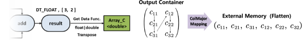
Figure 5: Extract data and map into a column-majored memory space.

It needs to be mentioned that the actual information passed to the set/get data functions is a pointer that specifies the data type (e.g., int, float or double), the array’s memory address, and the number of data indicating the size of this piece of memory. A more detailed explanation including the intrinsic version of setting and getting data functions can be found in the API document (B).

⬇

1// Header files

2#include "predictor.h" // Predictor header

3#include <vector> // C++ standard header

4

5int main(int argc, char const *argv[]) {

6 // Load Model:

7 Predictor pd("simple_graph_tf2.pb"); // Model’s path or filename

8

9 // Register node:

10 // Inputs:

11 // Predictor::INPUT_NODE is the node type enumerate

12 pd.regist_node("input_a", Predictor::INPUT_NODE);

13 pd.regist_node("input_b", Predictor::INPUT_NODE);

14 // Outputs:

15 // Predictor::OUTPUT_NODE is the node type enumerate

16 pd.regist_node("result", Predictor::OUTPUT_NODE);

17

18 // Set the number of data instances (n=3)

19 pd.set_data_count(3);

20

21 // Create external source of input/output data array:

22 // Inputs:

23 std::vector<float> vec_input1_float = {1.1, 2.2, 3.3, 4.4, 5.5, 6.6};

24 std::vector<int> vec_input2_float = {6, 5, 4, 3, 2, 1};

25 // Outputs:

26 std::vector<double> vec_out_float(6);

27

28 // Set data for input nodes

29 pd.set_node_data("input_a", vec_input1);

30 pd.set_node_data("input_b", vec_input2);

31

32 // Run model

33 pd.run();

34

35 // Get output into the target container

36 pd.get_node_data("result", vec_out, Predictor::ColumnMajor);

37

38 // Check results, expected calculation results:

39 // vec_out: [7.1, 7.3, 7.5, 7.2, 7.4, 7.6]

40 // [C11, C21, C31, C12, C22, C32]

41 return 0;

42}

Listing 2: Minimal example to run A + B model in C++

3 Tutorial Cases

Two tutorial cases are presented in this section. The first case is to solve a simple heat transfer problem using a data-driven approach, which demonstrates the basic process to invoke an ML model’s prediction within a CFD program by modifying the Laplacian solver in OpenFOAM. The second tutorial replicates the methodology of the iterative ML-RANS framework [35, 36] in OpenFOAM, and further migrates the turbulence model to the CFL3D code. The simulation cross validates the feasibility of the ML-RANS system, as both CFD codes have achieved converged solutions identical to the high-fidelity database of turbulent channel flow.

3.1 A Heat Transfer Problem

The predictor library is first applied in a modified OpenFOAM Laplacian solver (source code can be found in the folder: heat_transfer) to solve a one-dimensional steady heat transfer problem with radioactive and convective heat sources [27], which can be defined by the following equation:

$$\frac{d^{2}T}{dx^{2}}=\varepsilon(T)\left(T_{\infty}^{4}-T^{4}\right)+h\left(T_{\infty}-T\right),$$ (1)

in which, $T$ is the temperature, $x$ is the space coordinate with range: $x\in[0,1]$, $T_{\infty}$ is the temperature of the heating source, $h$ is a constant convection coefficient: $h=0.5$, and $\varepsilon(T)$ is the emissivity determined by the local temperature:

$$\varepsilon(T)=\left[1+5\sin\left(\frac{3\pi}{200}T\right)+\exp(0.02T)\right]\times 10^{-4}$$ (2)

However, the emissivity-temperature relation described by Eq. 2 is supposed to be unknown to the solver, and a model is therefore needed to establish the relation between emissivity and temperature. In the present case, the training data is generated by adding a zero-mean Gaussian noise, $\mathcal{N}\left(0,\sigma^{2}\right)$, to Eq. 2 ($\sigma$ is taken to be 0.3). The emissivity analytical formula and the training data can be seen in Fig. 6.

To solve Eq. 1, a traditional modeling strategy often attempts to find out an empirical analytical relation with coefficients regressed from the observed data, so that the relation can be solved as a part of the governing equations. For this tutorial, a data-driven approach is adopted in the modeling process, where a two-layer NN is trained to approximate the emissivity-temperature relation. The temperature is taken as the input, and the emissivity is the output. The hyper-parameters for the NN training are listed in Table. 2. The NN-estimated emissivity model compared to the theoretical truth and the training data is shown in Fig. 6.

Table 2: Hyper-parameters of emissivity-temperature NN

Hyperparameters	Recommend Values
Number of Hidden Layers	2
Number of Nodes per Layer	32
Activation Function	tanh
Optimizer	Adam
Learning Rate	0.001
L1 Regularization	3e-05
L2 Regularization	8e-04
Epoch Numbers	5000

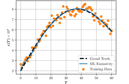
Figure 6: Comparison of machine-learned function, the true distribution and data with noises.

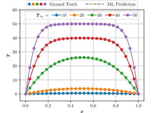
Figure 7: Temperature distribution of the true analytical model and ML model.

The trained model is then deployed in OpenFOAM to solve Eq. 1 and get the temperature distribution, using the modified Laplacian solver of the OpenFOAM. The comparison of the temperature between the ML and the analytical models is shown in Fig. 7, where the temperature of the heat source is set to be $T_{\infty}=10,20,...,50$. As can be seen from the figure, the ML model achieves a remarkable accuracy, indicating the ML model successfully learned the relation described by Eq. 2 via the training process, and the deployment of the model to the OpenFOAM effectively solves the heat transfer problem. This training and deployment process can be applied to solve a real engineering problem, where there is no analytical formula to describe the unknown relation and only some measured data are available.

3.2 The ML-RANS model in OpenFOAM and CFL3D

The training methodology of the iterative ML-RANS framework [35, 36] is replicated, in which, NN is adopted to model the effect of turbulence in channel flows. The NN model is then deployed through the predictor library in two classic CFD codes, OpenFOAM and CFL3D, written with C++ and Fortran, respectively. The relevant codes including the training scripts, modified solvers and simulation cases can be viewed in the repository (see folder: turbulent_channel and CFL3D-Extension for details).

The ML-RANS framework is designed with a built-in consistency to reproduce the high-fidelity training data in the a posteriori simulations. The model has been tested and assessed in engineering applications, and it showed an improved performance against conventional models [43]. The computational procedures are shown in Fig. 8, where the idea is to incorporate transport equations of a conventional turbulence model to provide auxiliary quantities for both training and prediction. Such quantities are combined with mean flow variables to form the dimensionless input features for the ML model. Meanwhile, the form of the closure term is chosen based on the conditioning analysis [44] of the Reynolds-averaged Navier–Stokes (RANS) equations, and the actual effect of the closure term is verified by forward solving the RANS equations based on the closure’s pre-mapped frozen distribution. With a proper normalization of the input and output data, the ML model can be trained and then loaded by CFD solvers to perform the a posteriori simulations.

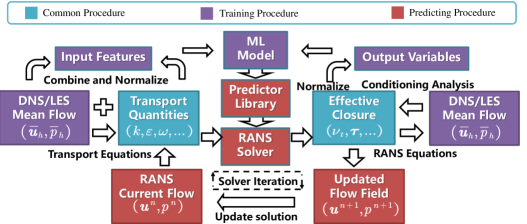
Figure 8: The iterative ML-RANS framework with consistent computational procedure.

The DNS channel flow at $Re_{\tau}=\left\{180,395,640,1020\right\}$ from Abe et al. [45, 46] are used as training cases, in which, the Reynolds number, $Re_{\tau}$, is defined as:

$$Re_{\tau}=\frac{u_{\tau}h}{\nu}$$ (3)

where $u_{\tau}$ is the friction velocity, $h$ is the half height of the channel, and $\nu$ is the molecular kinematic viscosity.

For each independent training case, the input and output data are obtained with the following steps. First, the DNS mean flow fields (i.e., velocity and pressure fields for incompressible flow) are interpolated to the computational mesh. The transport equations of the $k$–$\omega$ SST [47] model are then solved based on the frozen DNS mean field through the modified scalar transport solver in OpenFOAM, with turbulence kinetic energy $k$ and turbulence frequency $\omega$ being saved as auxiliary variables. Second, the eddy-viscosity field is calculated from DNS data as the effective closure term based on the conditioning analysis [44]. Finally, the saved $k$ and $\omega$ are adopted to perform a bounded normalization [36] of the input and output data, with their physical meanings and non-dimensional denominators listed in Table. 3. After generating training data for each case, the data from the four training cases are grouped together to train a four-layer NN (see Table. 4 for the training parameters). The eddy-viscosity used in the second step is calculated from the mean strain and Reynolds stress tensors as,

$$\nu_{t}=\left|\frac{\tau_{ij}S_{ij}}{2S_{ij}S_{ij}}\right|,$$ (4)

where $\tau_{ij}$ is the Reynolds stress tensor, $S_{ij}$ is the strain rate tensor, and the Einstein summation is applied for repeated indices.

Table 3: Non-dimensional input and output data definition for the ANN

Variable type	Raw definition	Normalize factor	Normalized form$\star$	Description
Input feature	$k$	$0.5u_{i}u_{i}$ $\dagger$	$50k/(50k+u_{i}u_{i})$ $\ddagger$	turbulence intensity
Input feature	$k/\omega$	$\nu$	$k/(k+50\nu\omega)$	estimated eddy viscosity
Label data	$\nu_{t}$	$k/\omega$	$5\nu_{t}/(5\nu_{t}+3k/\omega)$	true eddy viscosity

• The normalization strategy [36] takes a relative division $\bar{q_{i}}=|q_{i}|/(|{q_{i}|}+|\tilde{q_{i}}|)$, where $\bar{q_{i}}$ is the normalized variable, $q_{i}$ is the raw variable, and $\tilde{q_{i}}$ is the normalize factor.

• The value of $q_{i}$ and $\tilde{q_{i}}$ are adjusted with constant multiplier, ensuring $\bar{q_{i}}$ a uniform distribution between 0 and 1 within the range of training data.

• $0.5u_{i}u_{i}$ is the kinetic energy of mean flow, where $u_{i}$ is the velocity vector.

Table 4: Hyper-parameters of the NN in ML-RANS framework

Hyperparameters	Recommend Values
Number of Hidden Layers	3
Number of Nodes per Layer	24
Activation Function	tanh
Optimizer	Adam
Learning Rate	0.002
L1 Regularization	4e-06
L2 Regularization	6e-06
Epoch Numbers	5000

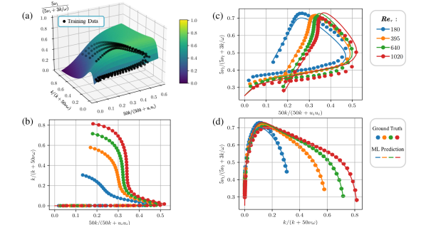
Figure 9: A priori performance of the ML model: (a) ML predicted surface and training data distribution in 3D frame: $x$-$y$ plane for input features, $z$ axis for output value. (b) 2D projections for $x$-$y$ plane of input features. (c) Comparison of ML predictions and training data in 2D projections for $x$-$z$ plane and (d) for $y$-$z$ plane.

The ML model’s a priori performance is shown in Fig. 9. Fig. 9.(a) shows the predicted curved surface of the NN compared with the training data, in which the $x$-axis stands for the first input feature, $\bar{q_{1}}=50k/(50k+u_{i}u_{i})$, and the $y$-axis is the second input feature, $\bar{q_{2}}=k/(k+50\nu\omega)$. The outputted variable, $\bar{\nu_{t}}=5\nu_{t}/(5\nu_{t}+3k/\omega)$, is the $z$-axis. Fig. 9.(b), (c), and (d) further show the 2D projection of (a) along the $z$, $y$, and $x$-axes, in which the output from the ML model is compared with the ground truth under the same input data. From the a priori results, we can see that the NN finally obtains a surface with the training data falling on closely, and the smoothness and flatness of the surface are satisfying. The output’s variation patterns with respect to each independent input feature are also accurately captured, as the predicted lines perfectly matched the training data in the $y$-$z$ plane (Fig. 9.(d)). In the $x$-$z$ plane, the ML returns the averaged curve of the training data in the bottom half of the figure. This is because the inputs of the four cases overlap in this region (shown as an overlapped straight line in Fig. 9(b) at $y\approx 0$), which does not provide enough separated distance to obtain distinguished outputs.

The trained model is then deployed into OpenFOAM and CFL3D through the C++ and Fortran APIs of the predictor library. The eddy-viscosity calculated from the $k$–$\omega$ SST model in the two CFD codes is then substituted with the ML model’s prediction at each iteration step. The iteration stops until the residuals of the mean flow field, turbulence quantities, and the closure term reach certain criteria. The a posteriori simulations are conducted at $Re_{\tau}=\left\{180,395,640,830,1020,1340,1670,2000\right\}$, where cases at $Re_{\tau}=\left\{180,395,640,1020\right\}$ and $Re_{\tau}=2000$, are compared with DNS data [45, 46] to evaluate the model’s interpolation and extrapolation performance, respectively. The results at intervening Reynolds numbers (i.e., $Re_{\tau}=\left\{830,1340,1670,\right\}$) indicates that the ML model works properly within a certain range.

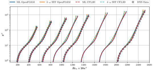
Figure 10: The velocity profiles of the series a posteriori simulations.

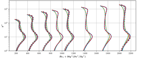
Figure 11: The $y^{+}\partial u^{+}/\partial y^{+}$ profiles of the series a posteriori simulations.

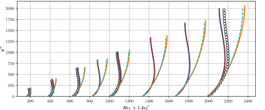
Figure 12: The eddy-viscosity profiles of the series a posteriori simulations.

This series of cases adopt a quasi-2D grid with 1153 $\times$ 101 nodes in the wall-normal and streamwise direction respectively, which ensures the grid resolution at the wall, $y_{1}^{+}\leq 1$, at the highest Reynolds number (i.e., $Re_{\tau}=2000$). The results from different models and CFD codes are compared in Figs. 10, 11, and 12, which respectively present profiles of velocity, velocity gradient, and eddy-viscosity. More specifically, the results from the case at $Re_{\tau}=640$ are shown separately to highlight the performance of the ML model in Figs. 13 and  14.

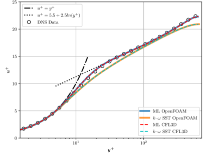
Figure 13: The velocity profile of the a posteriori simulation at $Re_{\tau}=640$.

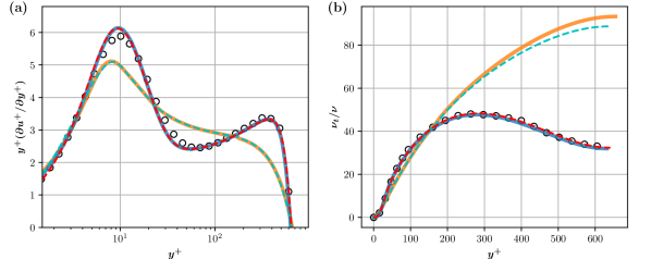
Figure 14: The $y^{+}\partial u^{+}/\partial y^{+}$ and eddy-viscosity profiles of the a posteriori simulation at $Re_{\tau}=640$.

It can be seen from Figs. 10, 11, and 12 that the results of the ML model from two different CFD codes overlap perfectly with each other, meaning that the implementation of the ML library is code-independent. The ML model presents improved results against the conventional $k$–$\omega$ SST model, which agrees with the previous result of Liu et al. [35, 36]. Although the implementation of the CFD algorithms differs significantly between the two CFD codes, the reproducibility of the ML-RANS framework is adequately demonstrated through the predictor library.

The predictor library can be deployed to parallel CFD solvers based on domain decomposition and communication using the message passing interface (MPI). Under this parallel strategy, each thread will load an independent predictor to handle the ML prediction within its local subdomain. To evaluate the predictor’s influence on the parallel performance, the simulation of channel flow with 1-16 MPI threads is conducted. The elapsed time in a single iteration and the extra time cost from the ML prediction in both CFD codes are shown in Table. 5, from which we note that incorporation of the ML model brings an extra 10% – 15% time cost compared with a conventional turbulence model. The speed-up ratio is demonstrated in Fig. 15, where no obvious difference between the ML model and $k$–$\omega$ SST model is observed. Therefore, the parallel efficiency is not influenced by incorporating the predictor library.

Table 5: Elapsed time in a single iteration for $k$–$\omega$ SST and ML model in channel flow under parallel configuration

Blocks	OpenFOAM			CFL3D *
	ML Model	$k$–$\omega$ SST	ML Cost **	ML Model	$k$–$\omega$ SST	ML Cost **
1	0.308s	0.277s	11.19%	0.422s	0.367s	14.99%
2	0.158s	0.141s	11.90%	0.216s	0.189s	14.55%
4	0.083s	0.074s	12.16%	0.112s	0.099s	13.56%
8	0.050s	0.044s	13.64%	0.063s	0.056s	12.76%
16	0.034s	0.030s	14.33%	0.042s	0.037s	12.31%

• CFL3D needs one extra core as the host of MPI slaves, for example, 17 cores are needed in the 16-block case.

• The extra percentage of time cost compared with $k$–$\omega$ SST model.

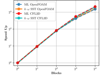
Figure 15: The parallel speed-up ratio of ML model and $k$–$\omega$ SST model on OpenFOAM and CFL3D.

4 Conclusion and Further Improvements

A predictor library is developed to deploy NN to CFD software conveniently. Using the Pimpl strategy, the library isolates the implementation details and achieves a pure-method class that can be easily extended to other languages. The library currently provides language-level APIs for C++ and Fortran, and high-level modules for OpenFOAM and CFL3D. The simplified APIs for loading models, setting the parallel options, and the data I/O functions enhanced the compatibility with most CFD programs.

The basic usage of the library is first demonstrated through a simple A + B example, and further explained in modeling a 1-D heat transfer problem. The library is then applied in OpenFOAM and CFL3D to simulate turbulent channel flow using the ML model accounting for the effect of turbulence. The results are shown to be independent of CFD software. The incorporation of the library does not influence the parallel efficiency of a CFD code. This newly developed ML predictor library could largely promote the deployment of ML models in mainstream CFD software.

Further improvement of the predictor can be made in three aspects. First, the library can be applied to other types of partial differential equation solvers for wider communities. Second, more backends should be supported, such as loading PyTorch and driving a Python interpreter, to provide more flexible ML support. Finally, the ML acceleration can be adapted to different parallel structures. For example, the ML prediction can be executed on GPU in a server-client mode in a heterogeneous computing system.

Appendix A Installation Guide

C++ Core Predictor:

In the third_party directory of the code repository, a bash script for downloading the necessary dependencies is available: DownloadThirdParty.sh. Users can simply execute the script:

⬇

$ cd Predictor-Core/third_party

$ sh DownloadThirdParty.sh

in which, the major dependencies are TensorFlow C API binary library and Eigen numerical template library. The former is the core functioning library to call ML prediction whereas the latter could enable efficient I/O option with SIMD (Single Instruction/Multiple Data) [48] operations. One can also download the dependencies with the following links (no need to compile the dependencies) manually:

• libtensorflow.so

• Eigen

Two environment variables: MY_TF_HOME and MY_EIGEN_HOME are needed to specify the location of these third-party libraries. The bash script: activate.sh could quickly set the environment variables if the download script is executed:

⬇

$ source activate.sh

Otherwise users needs to set them manually via:

⬇

$ export MY_EIGEN_HOME=path/to/your/eigen/dir

$ export MY_TF_HOME=path/to/your/TF/dir/

Then the predictor library is ready to be compiled via (tested passed by GNU compiler ver 7.3.1):

⬇

$ make cxxso # C++ library

$ make cxxtest # C++ test program loading A+B

$ make run # run the test program

In addtion, two macro flags can be specified in the Makefile to achieve special usage:

⬇

-D_CPU_SERIAL # default run serially, otherwise will use all available CPUs

-D_DEBUG # print error messages if not properly used

Fortran Interface:

With C++ core predictor compiled, one with GNU Fortran compiler [39] could directly compile the Fortran interface and its test program via:

⬇

$ make f90so # Fortran predictor library

$ make f90test # Fortran test program loading A+B

$ make runf # run the Fortran test program

OpenFOAM Module:

Apart from the C++ core predictor library, the OpenFOAM module needs to be compiled within an activated wmake environment, which means OpenFOAM installation is required first. The module supports OpenFOAM version $\geq$ 4, and can be compiled and tested via:

⬇

$ cd OpenFOAM-Extension # Go to the OF Extension dir

$ make ofso # OpenFOAM module library

$ make oftest # OpenFOAM test program loading A+B

$ make runof # run the OpenFOAM test program

Fortran CFD Module (i.e., the CFL3D module):

The self-developed CFL3D solver with ML taking over the prediction of eddy-viscosity can be compiled via:

⬇

$ cd CFL3D-Extension # Go to the OF Extension dir

$ make cfl3d_seq_ori # Original solver serial version

$ make cfl3d_mpi_ori # Original solver parallel version

$ make cfl3d_seq_ml # ML-RANS solver serial version

$ make cfl3d_mpi_ml # ML-RANS solver parallel version

Instead of compiling the module into an independent library, a Fortran 90 format module template is provided to compile with CFD program together. Users are recommended to modify the template following the instructions. This template module design pattern is tested as compatible with fixed format (*.F) and free format (*.F90) because it only interacts with the arrays without allocating extra memory spaces in the main CFD program. All the other intermediate arrays and class instances are maintained by the module itself. Therefore the risk of memory leak in a legacy Fortran program can be avoided.

Appendix B Detailed API Documents

This appendix records the entire document of the APIs in C++, Fortran, and OpenFOAM extension. The extension module for CFL3D is shown as a template to provide a solution dealing with legacy CFD code. The same A + B model is adopted in examples for C++, Fortran, and OpenFOAM for a better understanding. For C++ and Fortran, the alternative APIs are listed after the code example with the specified step ID for a more customized usage.

The two different formats of TensorFlow model can be generated by simply executing createmodel_AplusB.py, where the TensorFlow version is automatically detected to match the API difference between TensorFlow version 1 and 2:

⬇

$ python3 createmodel_AplusB.py PB # Save model in Protobuf format

$ python3 createmodel_AplusB.py SavedModel # Save model in SavedModel format

The model will finally be saved with the following filename:

⬇

simple_graph_tf1.pb # TF1 saved *.pb format

simple_graph_tf2.pb # TF2 saved *.pb format

saved_tf1_model # TF1 SavedModel format (Normally by Estimator)

saved_tf2_model # TF2 SavedModel format (Normally by TF2 Keras)

B.1 C++ Core Predictor Class APIs

The C++ code example deploying the A + B model is shown in Listing 3, in which, the necessary steps, with their function prototypes and locations in the code example, are marked in Table. 6:

Table 6: ID, function prototypes and locations of necessary steps in C++

Step ID	Usage	Function Prototype *	Location
C01	Load Model	Predictor(std::string PBfile)	06-07
C02	Register Nodes	regist_node(std::string node_name, Predictor::NodeType tp)	09-16
C03	Set Data Counts	set_data_count(int n_data)	18-19
C04	Set Input Data	set_node_data(std::string node_name, std::vector<T>& data)	28-30
C05	Run Model	run()	32-33
C06	Get Output Data	get_node_data(std::string node_name, std::vector<T>& data)	35-36

• The function prototypes are all under public class: class Predictor. Therefore, the full reference of functions, for example for C01, should be: Predictor::Predictor(std::string PBfile)

Basically, the code example is similar to the code shown in Sec. 2.3.2, the only difference is that the output array is not transposed in this case, which reads:

⬇

1// Header files

2#include "predictor.h" // Predictor header

3#include <vector> // C++ standard header

4

5int main(int argc, char const *argv[]) {

6 // Load Model:

7 Predictor pd("simple_graph_tf2.pb"); // Model’s path or filename

8

9 // Register node:

10 // Inputs:

11 // Predictor::INPUT_NODE is the node type enumerate

12 pd.regist_node("input_a", Predictor::INPUT_NODE);

13 pd.regist_node("input_b", Predictor::INPUT_NODE);

14 // Outputs:

15 // Predictor::OUTPUT_NODE is the node type enumerate

16 pd.regist_node("result", Predictor::OUTPUT_NODE);

17

18 // Set the number of data instances (n=3)

19 pd.set_data_count(3);

20

21 // Create external source of input/output data array:

22 // Inputs:

23 std::vector<float> vec_input1_float = {1.1, 2.2, 3.3, 4.4, 5.5, 6.6};

24 std::vector<int> vec_input2_float = {6, 5, 4, 3, 2, 1};

25 // Outputs:

26 std::vector<double> vec_out_float(6);

27

28 // Set data for input nodes

29 pd.set_node_data("input_a", vec_input1);

30 pd.set_node_data("input_b", vec_input2);

31

32 // Run model

33 pd.run();

34

35 // Get output into the target container

36 pd.get_node_data("result", vec_out);

37

38 // Check results, expected calculation results:

39 // vec_out: [7.1, 7.3, 7.5, 7.2, 7.4, 7.6]

40 // [C11, C21, C31, C12, C22, C32]

41 return 0;

42}

Listing 3: Minimal example to run A + B model in C++

Entire API list for C++:

• C01: Loading Model:

  • Predictor(std::string pbfile)

    • pbfile – the file name of the PB graph (i.e.,simple_graph_tf2.pb).

    Class constructor, to create the Predictor object from a *.pb format.

  • Predictor(std::string folder, std::string tag)

    • folder – the directory of the SavedModel format (this format itself is a folder).

    • tags – tags label within a SavedModel format, by default is serve.

    Class constructor, to create the Predictor object from a SavedModel format.

  • Predictor(std::string pbfile, uint8_t para_intra, uint8_t para_inter)

    • pbfile – the name of the PB graph (i.e.,simple_graph_tf2.pb).

    • para_intra – number of threads for internal parallelization (e.g., matrix multiplication and reduce sum).

    • para_inter – number of threads for operations independent with each other.

    Class constructor, to create the Predictor object from a *.pb format with parallelization configs. If both para_intra and para_inter are set to be 0, the system will pick an appropriate number. If they are set to be 1, the predictor will run model serially (an easy way to cooperate with MPI pattern in CFD codes).

  • Predictor(std::string folder, std::string tag, uint8_t para_intra, uint8_t para_inter)

    • folder – the directory of the SavedModel format (this format itself is a folder).

    • tags – tags label within a SavedModel format, by default is serve.

    • para_intra – number of threads for internal parallelization (e.g., matrix multiplication and reduce sum).

    • para_inter – number of threads for operations independent with each other.

    Class constructor, to create the Predictor object from a SavedModel format with parallelization configs. If both para_intra and para_inter are set to be 0, the system will pick an appropriate number. If they are set to be 1, the predictor will run model serially (an easy way to cooperate with MPI pattern in CFD codes).

• C02: Register Nodes:

  • regist_node(std::string node_name, NodeType type)

    • node_name – the name of the node to be registered as input or output.

    • type – the enumerate to specify node type, the available options are:

      • Predictor::INPUT_NODE – to register node as input.

      • Predictor::OUTPUT_NODE – to register node as output.

    To register input and output node for feeding and extracting data.

• C03: Set Data Counts:

  • set_data_count(int n_data)

    • n_data – the number of data instances.

    To set the number of data instances to substitute the unknown dimension of input/output tensors. For example, in the A + B example, the input/output shapes are all [-1, 2], the function could set the unknown -1 into concrete value so that the inner data containers can be created.

• C04: Set Input Data:

  • set_node_data(std::string node_name, std::vector<T>& data)

    • node_name – the name of the input node to be fed with external data.

    • data – the external data defined with C++ STL library (i.e., std::vector)

    To feed the internal input data container registered under node_name with external data source hold by a C++ standard template library (STL) std::vector. If the data type of the internal container and external source are different, this function would automatically cast the datatype to resolve the difference.

  • set_node_data(std::string node_name, std::vector<T>& data, DataLayout layout)

    • node_name – the name of the input node to be fed with external data.

    • data – the external data defined with C++ STL library (i.e., std::vector)

    • layout – the enumerate to specify whether the memory layout is transposed, the available options are:

      • Predictor::RowMajor – to hold the original memory sequence of the external data source.

      • Predictor::ColumnMajor – to perform matrix transpose while set data to internal container.

    To feed the internal input data container registered under node_name with external data source hold by a C++ standard template library (STL) std::vector. If the data type of the internal container and external source are different, this function would automatically cast the datatype to resolve the difference. The memory layout would be changed during the mapping process if Predictor::ColumnMajor is passed to the function.

  • set_node_data(std::string node_name, std::vector<T>& data, DataLayout layout,
CopyMethod method)

    • node_name – the name of the input node to be fed with external data.

    • data – the external data defined with C++ STL library (i.e., std::vector)

    • layout – the enumerate to specify whether the memory layout is transposed, the available options are:

      • Predictor::RowMajor – to hold the original memory sequence of the external data source.

      • Predictor::ColumnMajor – to perform matrix transpose while set data to internal container.

    • method – the enumerate to specify the copy method to the internal container:

      • Predictor::Simple – to copy/cast the arrays element-wise through C++ loop (possibly cache miss).

      • Predictor::Eigen – to copy/cast the arrays via Eigen library (SIMD is enabled).

    To feed the internal input data container registered under node_name with external data source hold by a C++ standard template library (STL) std::vector. If the data types of the internal container and external source are different, this function would automatically cast the datatype to resolve the difference. The memory layout would be changed during the mapping process if Predictor::ColumnMajor is passed to the function. The copy/cast procedure could be accelerated via Eigen library by specifying Predictor::Eigen options.

  • set_node_data(std::string node_name, T* p_data, int array_size)

    • node_name – the name of the input node to be fed with external data.

    • p_data – the pointer to the first element of external data array.

    • array_size – the number of data elements of the external data array.

    To feed the internal input data container registered under node_name with external data source specified by the pointer to the array and the number of data elements. If the data types of the internal container and external source are different, this function would automatically cast the datatype to resolve the difference.

  • set_node_data(std::string node_name, T* p_data, int array_size, DataLayout layout)

    • node_name – the name of the input node to be fed with external data.

    • p_data – the pointer to the first element of external data array.

    • array_size – the number of data elements of the external data array.

    • layout – the enumerate to specify whether the memory layout is transposed, the available options are:

      • Predictor::RowMajor – to hold the original memory sequence of the external data source.

      • Predictor::ColumnMajor – to perform matrix transpose while set data to internal container.

    To feed the internal input data container registered under node_name with external data source specified by the pointer to the array and the number of data elements. If the data types of the internal container and external source are different, this function would automatically cast the datatype to resolve the difference. The memory layout would be changed during the mapping process if Predictor::ColumnMajor is passed to the function.

  • set_node_data(std::string node_name, T* p_data, int array_size, DataLayout layout,
CopyMethod method)

    • node_name – the name of the input node to be fed with external data.

    • p_data – the pointer to the first element of external data array.

    • array_size – the number of data elements of the external data array.

    • layout – the enumerate to specify whether the memory layout is transposed, the available options are:

      • Predictor::RowMajor – to hold the original memory sequence of the external data source.

      • Predictor::ColumnMajor – to perform matrix transpose while set data to internal container.

    • method – the enumerate to specify the copy method to the internal container:

      • Predictor::Simple – to copy/cast the arrays element-wise through C++ loop (possibly cache miss).

      • Predictor::Eigen – to copy/cast the arrays via Eigen library (SIMD is enabled).

    To feed the internal input data container registered under node_name with external data source specified by the pointer to the array and the number of data elements. If the data types of the internal container and external source are different, this function would automatically cast the datatype to resolve the difference. The memory layout would be changed during the mapping process if Predictor::ColumnMajor is passed to the function. The copy/cast procedure could be accelerated via Eigen library by specifying Predictor::Eigen options.

• C05: Run Model:

  • run()

    To run the model prediction, the result will be stored in the internal data container holding the model’s output.

• C06: Get Output Data:

  • get_node_data(std::string node_name, std::vector<T>& data)

    • node_name – the name of the output node’s data to be extracted to external array.

    • data – the external data defined with C++ STL library (i.e., std::vector)

    To extract the data stored in the the internal output data container registered under node_name into external data array hold by a C++ standard template library (STL) std::vector. If the data types of the internal container and external source are different, this function would automatically cast the datatype to resolve the difference.

  • get_node_data(std::string node_name, std::vector<T>& data, DataLayout layout)

    • node_name – the name of the output node’s data to be extracted to external array.

    • data – the external data defined with C++ STL library (i.e., std::vector)

    • layout – the enumerate to specify whether the memory layout is transposed, the available options are:

      • Predictor::RowMajor – to hold the original memory sequence of the external data source.

      • Predictor::ColumnMajor – to perform matrix transpose while set data to internal container.

    To extract the data stored in the the internal output data container registered under node_name into external data array hold by a C++ standard template library (STL) std::vector. If the data types of the internal container and external source are different, this function would automatically cast the datatype to resolve the difference. The memory layout would be changed during the mapping process if Predictor::ColumnMajor is passed to the function.

  • get_node_data(std::string node_name, std::vector<T>& data, DataLayout layout,
CopyMethod method)

    • node_name – the name of the output node’s data to be extracted to external array.

    • data – the external data defined with C++ STL library (i.e., std::vector)

    • layout – the enumerate to specify whether the memory layout is transposed, the available options are:

      • Predictor::RowMajor – to hold the original memory sequence of the external data source.

      • Predictor::ColumnMajor – to perform matrix transpose while set data to internal container.

    • method – the enumerate to specify the copy method to the internal container:

      • Predictor::Simple – to copy/cast the arrays element-wise through C++ loop (possibly cache miss).

      • Predictor::Eigen – to copy/cast the arrays via Eigen library (SIMD is enabled).

    To extract the data stored in the the internal output data container registered under node_name into external data array hold by a C++ standard template library (STL) std::vector. If the data type of the internal container and external source are different, this function would automatically cast the datatype to resolve the difference. The memory layout would be changed during the mapping process if Predictor::ColumnMajor is passed to the function. The copy/cast procedure could be accelerated via Eigen library by specifying Predictor::Eigen options.

  • get_node_data(std::string node_name, T* p_data, int array_size)

    • node_name – the name of the output node’s data to be extracted to external array.

    • p_data – the pointer to the first element of external data array.

    • array_size – the number of data elements of the external data array.

    To extract the data stored in the the internal output data container registered under node_name into external data array specified by the pointer to the array and the number of data elements. If the data type of the internal container and external source are different, this function would automatically cast the datatype to resolve the difference.

  • get_node_data(std::string node_name, T* p_data, int array_size, DataLayout layout)

    • node_name – the name of the output node’s data to be extracted to external array.

    • p_data – the pointer to the first element of external data array.

    • array_size – the number of data elements of the external data array.

    • layout – the enumerate to specify whether the memory layout is transposed, the available options are:

      • Predictor::RowMajor – to hold the original memory sequence of the external data source.

      • Predictor::ColumnMajor – to perform matrix transpose while set data to internal container.

    To extract the data stored in the the internal output data container registered under node_name into external data array specified by the pointer to the array and the number of data elements. If the data type of the internal container and external source are different, this function would automatically cast the datatype to resolve the difference. The memory layout would be changed during the mapping process if Predictor::ColumnMajor is passed to the function.

  • get_node_data(std::string node_name, T* p_data, int array_size, DataLayout layout,
CopyMethod method)

    • node_name – the name of the output node’s data to be extracted to external array.

    • p_data – the pointer to the first element of external data array.

    • array_size – the number of data elements of the external data array.

    • layout – the enumerate to specify whether the memory layout is transposed, the available options are:

      • Predictor::RowMajor – to hold the original memory sequence of the external data source.

      • Predictor::ColumnMajor – to perform matrix transpose while set data to internal container.

    • method – the enumerate to specify the copy method to the internal container:

      • Predictor::Simple – to copy/cast the arrays element-wise through C++ loop (possibly cache miss).

      • Predictor::Eigen – to copy/cast the arrays via Eigen library (SIMD is enabled).

    To extract the data stored in the the internal output data container registered under node_name into external data array specified by the pointer to the array and the number of data elements. If the data type of the internal container and external source are different, this function would automatically cast the datatype to resolve the difference. The memory layout would be changed during the mapping process if Predictor::ColumnMajor is passed to the function. The copy/cast procedure could be accelerated via Eigen library by specifying Predictor::Eigen options.

• Auxiliary Functions:

  • print_operations()

    To print all the node information (type and shape) in the loaded model.

  • print_operations(std::string node_name)

    • node_name – the name of node to print shape and type information.

    To print the node information (type and shape) with specified name in the loaded model.

B.2 Fortran Calling the Predictor Function

The Fortran APIs is a wrapper of the C++ predictor class through ISO_C_BINDING, which is supposed to be a necessary component in a GNU Fortran compiler. A minimal code example that closely replicates the C++ calling sequence is shown below (written in F90). The major subroutines with their locations in the example are listed in Table. 7. One difference between the C++ example is that in the data I/O process, the Fortran APIs adopt the pointer-and-data-number calling methods, since the Fortran’s array shape information is not naturally passed to C++ via ISO_C_BINDING.

Table 7: ID, function prototypes and locations of necessary steps in Fortran

Step ID	Usage	Function Prototype	Location
F01	Load Model	ptr = C_CreatePredictor(file_name) *	13-14
F02	Register Inputs	C_PredictorRegisterInputNode(ptr, in_node_name)	16-18
F03	Register Outputs	C_PredictorRegisterOutputNode(ptr, in_node_name)	20-21
F04	Set Data Counts	C_PredictorSetDataCount(ptr, n_data)	23-24
F05	Set Input Data	C_PredictorSetNodeData(ptr, in_node, input_arr , n_element)	26-28
F06	Run Model	C_PredictorRun(ptr)	30-31
F07	Get Output Data	C_PredictorGetNodeData(ptr, out_node, output_arr , n_element)	33-34
F08	Finalize Model	C_DeletePredictor(ptr)	39-40

• The type of the returned value should be declared as: type(c_ptr) :: ptr.

The Fortran code example to load the A + B model reads:

⬇

1program main

2use ml_predictor !The predictor module that declared all the function interfaces

3use iso_c_binding, only: c_ptr !C-pointer to the Predictor instance

4

5 implicit none

6 type(c_ptr) :: ptr ! C-pointer to the Predictor instance

7

8 ! External input/output arrays from fortran program (Support up to 6d)

9 real(kind=4), dimension(2,3) :: arr_a = reshape((/0.0, 1.1, 2.2, 3.3, 4.4, 5.5/), (/2,3/))

10 integer(kind=4), dimension(6) :: arr_b = (/5, 4, 3, 2, 1, 0/)

11 real(kind=8), dimension(3,2) :: arr_c = 0.0

12

13 ! Create predictor from *.pb

14 ptr = C_CreatePredictor("simple_graph_tf2.pb")

15

16 ! Register input nodes

17 call C_PredictorRegisterInputNode(ptr, "input_a")

18 call C_PredictorRegisterInputNode(ptr, "input_b")

19

20 ! Register output nodes

21 call C_PredictorRegisterOutputNode(ptr, "result")

22

23 ! Set number of data instances

24 call C_PredictorSetDataCount(ptr, 3)

25

26 ! Set the input data

27 call C_PredictorSetNodeData(ptr, "input_a", arr_a, 6)

28 call C_PredictorSetNodeData(ptr, "input_b", arr_b, 6)

29

30 ! Run the model

31 call C_PredictorRun(ptr)

32

33 ! Get the model output data into arr_c

34 call C_PredictorGetNodeData(ptr, "result", arr_c, 6)

35

36 ! Print the output

37 print*, "Calculation Result:", arr_c

38

39 ! Delete predictor when it is not used anymore

40 call C_DeletePredictor(ptr)

41

42end program main

Listing 4: Minimal example to run A + B model in Fortran

Entire API list for Fortran:

• F01: Loading Model:

  • ptr = C_CreatePredictor(file_name)

    • file_name – the Fortran CHARACTER array specifying the file name of the PB graph.

    To create the Predictor object from a *.pb format, which return the reference to the Predictor object, the return value, ptr should be defined as type(c_ptr)::ptr.

  • ptr = C_CreatePredictor(model_dir, tag)

    • model_dir – the Fortran CHARACTER array specifying the directory of the SavedModel format (this format itself is a folder).

    • tags – the Fortran CHARACTER array specifying the tags label within a SavedModel format, by default is serve.

    To create the Predictor object from a SavedModel format, which return the reference to the Predictor object, the return value, ptr should be defined as type(c_ptr)::ptr.

• F02: Register Inputs:

  • C_PredictorRegisterInputNode(ptr, in_node_name)

    • ptr – the C pointer reference to the created Predictor object.

    • in_node_name – the Fortran CHARACTER array specifying the name of the node to be registered as input.

    To register input node for feeding data.

• F03: Register Outputs:

  • C_PredictorRegisterOutputNode(ptr, out_node_name)

    • ptr – the C pointer reference to the created Predictor object.

    • out_node_name – the Fortran CHARACTER array specifying the name of the node to be registered as output.

    To register output node for extracting data.

• F04: Set Data Counts:

  • C_PredictorSetDataCount(ptr, n_data)

    • ptr – the C pointer reference to the created Predictor object.

    • n_data – the Fortran INTEGER variable specifying number of data instances.

    To set the number of data instances to substitute the unknown dimension of input/output tensors. For example, in the A + B example, the input/output shapes are all [-1, 2], the function could set the unknown -1 into concrete value so that the inner data containers can be created.

• F05: Set Input Data:

  • C_PredictorSetNodeData(ptr, in_node, input_arr , n_element)

    • ptr – the C pointer reference to the created Predictor object.

    • in_node – the Fortran CHARACTER array specifying the name of the input node to be fed with external data.

    • input_arr – the Fortran numerical array holding the external data, available data type: INTEGER, REAL(4) and REAL(8).

    • n_element – the Fortran INTEGER variable specifying the number of data elements of the external data array.

    To feed the internal input data container registered under in_node with external data array. Because the shape information of a Fortran array is lost when passing to a C library, so the total number of elements in the array needs to be specified. If the data type of the internal container and external source are different, this function would automatically cast the datatype to resolve the difference.

  • C_PredictorSetNodeDataTranspose(ptr, in_node, input_arr , n_element)

    • ptr – the C pointer reference to the created Predictor object.

    • in_node – the Fortran CHARACTER array specifying the name of the input node to be fed with external data.

    • input_arr – the Fortran numerical array holding the external data, available data type: INTEGER, REAL(4) and REAL(8).

    • n_element – the Fortran INTEGER variable specifying the number of data elements of the external data array.

    To feed the internal input data container registered under in_node with external data array. Because the shape information of a Fortran array is lost when passing to a C library, so the total number of elements in the array needs to be specified. If the data type of the internal container and external source are different, this function would automatically cast the datatype to resolve the difference. The memory layout would be tansposed during the mapping process.

• F06: Run Model:

  • C_PredictorRun(ptr)

    • ptr – the C pointer reference to the created Predictor object.

    To run the model prediction, the result will be stored in the internal data container holding the model’s output.

• F07: Get Output Data:

  • C_PredictorGetNodeData(ptr, out_node, output_arr , n_element)

    • ptr – the C pointer reference to the created Predictor object.

    • out_node – the Fortran CHARACTER array specifying the name of the output node’s data to be extracted to external array.

    • output_arr – the Fortran numerical array holding the external data, available data type: INTEGER, REAL(4) and REAL(8).

    • n_element – the Fortran INTEGER variable specifying the number of data elements of the external data array.

    To extract the data stored in the the internal output data container registered under out_node into external data array. Because the shape information of a Fortran array is lost when passing to a C library, so the total number of elements in the array needs to be specified. If the data type of the internal container and external source are different, this function would automatically cast the datatype to resolve the difference.

  • C_PredictorGetNodeDataTranspose(ptr, out_node, output_arr , n_element)

    • ptr – the C pointer reference to the created Predictor object.

    • out_node – the Fortran CHARACTER array specifying the name of the output node’s data to be extracted to external array.

    • output_arr – the Fortran numerical array holding the external data, available data type: INTEGER, REAL(4) and REAL(8).

    • n_element – the Fortran INTEGER variable specifying the number of data elements of the external data array.

    To extract the data stored in the the internal output data container registered under out_node into external data array. Because the shape information of a Fortran array is lost when passing to a C library, so the total number of elements in the array needs to be specified. If the data type of the internal container and external source are different, this function would automatically cast the datatype to resolve the difference. The memory layout would be tansposed during the mapping process.

• F08: Finalize Mode:

  • C_DeletePredictor(ptr)

    • ptr – the C pointer reference to the created Predictor object.

    To delete the Predictor object pointed by ptr, the manual finalization is needed because the resource created by C++ library would not be automatically released by Fortran.

B.3 OpenFOAM Predictor Module

The OpenFOAM module specifies all the available setting options in an OpenFOAM dictionary:

⬇

1model // Dictionary name, referenced by the constructor function

2{

3 readFromPB yes; // yes/no for PB/SavedModel

4 modelDirectory "models/simple_graph_tf2.pb";

5// tags "serve"; // only needed for SavedModel

6 copyMethod Eigen; // Eigen/Safe for SIMD/element-wise copy

7 layout ColMajor; // RowMajor or ColMajor

8 inputs ("input_a" "input_b"); // use space as separator

9 outputs ("result"); // use space as separator

10}

Listing 5: OpenFOAM dictionary to initialize predictor library

Therefore, the function call is simplified with just only the constructor function and prediction function (line 31 and 34 in the following codes). But calling the prediction is slightly different since OpenFOAM defines its own fundamental data structures. Two-level container (Foam::List) of the Foam::scalarField references need to be assembled. The outer-level Foam::List corresponds to the number of nodes, whereas the inner-level capacity corresponds to the known dimension of the node shape. For example in the A + B model, two independent nodes are registered as input nodes, so that the outer list capacity of the multi_inputs is two (line 36). The dimensions of the inner list (e.g., multi_inputs[0] in line 40) is two because the tensor shape of the input/output node is [-1, 2]. The exact code example can be found below:

⬇

1#include "scalarField.H" // Header from OpenFOAM

2#include "TF_OF_Predictor.H" // Header for TF_Predictor

3

4int main() {

5

6 // External OF fields ...

7

8 // create input field A (columns):

9 scalarField input_field_a_col1(3, scalar(0.0));

10 input_field_a_col1[0] = 0.0;

11 input_field_a_col1[1] = 2.2;

12 input_field_a_col1[2] = 4.4;

13 scalarField input_field_a_col2(3, scalar(0.0));

14 input_field_a_col2[0] = 1.1;

15 input_field_a_col2[1] = 3.3;

16 input_field_a_col2[2] = 5.5;

17

18

19 // create input field B (columns):

20 scalarField input_field_b_col1(3, scalar(0.0));

21 input_field_b_col1[0] = 5.0;

22 input_field_b_col1[1] = 3.0;

23 input_field_b_col1[2] = 1.0;

24 scalarField input_field_b_col2(3, scalar(0.0));

25 input_field_b_col2[0] = 4.0;

26 input_field_b_col2[1] = 2.0;

27 input_field_b_col2[2] = 0.0;

28

29 // create output field C (columns)

30 scalarField output_field_c_col1(3, scalar(0.0)); // output field for pb model column1

31 scalarField output_field_c_col2(3, scalar(0.0)); // output field for pb model column2

32

33

34 // Create the entry list for OF fields:

35 // PB format model:

36 Foam::List<Foam::List<scalarField*>> multi_inputs(2);

37 Foam::List<Foam::List<scalarField*>> multi_outputs(1);

38

39 // For input_a:

40 multi_inputs[0].append(&input_field_a_col1);

41 multi_inputs[0].append(&input_field_a_col2);

42

43 // For input_b:

44 multi_inputs[1].append(&input_field_b_col1);

45 multi_inputs[1].append(&input_field_b_col2);

46

47 // For output_c:

48 multi_outputs[0].append(&output_field_c_col1);

49 multi_outputs[0].append(&output_field_c_col2);

50

51

52 Info << "Creating TF_OF_Predictor\n" << endl;

53 TF_OF_Predictor pd = TF_OF_Predictor("constant/TF_Predictor_Dict", "model_pb_2D");

54

55

56 Info << "Running the models \n" << endl;

57 pd.predict(multi_inputs, multi_outputs);

58

59 Info << "Print the running results\n" << endl;

60 Info << "Results of column 1: \n"

61 << input_field_a_col1 << " + " << input_field_b_col1 << " = " << output_field_c_col1 << endl;

62

63 Info << "Results of column 2: \n"

64 << input_field_a_col2 << " + " << input_field_b_col2 << " = " << output_field_c_col2 << endl;

65

66 return 0;

67}

Listing 6: Minimal example to run A + B model in OpenFOAM

Entire API list for OpenFOAM Module:

• OF01: Model Initialization:

  • TF_OF_Predictor()

    To create the TF_OF_Predictor object from the OpenFOAM dictionary stored in default directory. The default file path of the dictionary is constant/TF_Predictor_Dict, and the settings are under the default dictionary name, model.

  • TF_OF_Predictor(std::string Model_name)

    • Model_name – the name of the dictionary the model will be launched under its setting options.

    To create the TF_OF_Predictor object from the OpenFOAM dictionary stored in default directory. The default file path of the dictionary is constant/TF_Predictor_Dict, and the settings are under the dictionary name, Model_name.

  • TF_OF_Predictor(std::string Dict_dir, std::string Model_name)

    • Dict_dir – the OpenFOAM dictionary file holding the dictionaries of the settings of the TF_OF_Predictor.

    • Model_name – the name of the dictionary the model will be launched under its setting options.

    To create the TF_OF_Predictor object from the OpenFOAM dictionary stored in Dict_dir, and the settings are under the dictionary name, Model_name.

• OF02: Model Prediction:

  • predict(Foam::List<Foam::scalarField*>& inputs,
Foam::List<Foam::scalarField*>& outputs)

    • inputs – the reference container holding the references of input scalarField for a single-input-output model.

    • outputs – the reference container holding the references of output scalarField for a single-input-output model.

    To perform prediction of a single-input-output model, which means the number of the input nodes and output nodes are both one. In this case, the capacity of the reference container corresponds to the known dimension of the node shape. For example, if the node shape is [-1, 2, 3], then the reference container needs to have $2\times 3=6$ references of scalarField.

  • predict(Foam::List<Foam::List<Foam::scalarField*>> & multi_inputs,
Foam::List<Foam::List<Foam::scalarField*>> & multi_outputs)

    • inputs – the two-level reference container holding the references of input scalarField for a multiple-input-output model.

    • outputs – the two-level reference container holding the references of output scalarField for a multiple-input-output model.

    To perform prediction of a multiple-input-output model, which means model has more than one input nodes or output nodes. In this case, the outer-level capacity of the two-level reference container equals to the number of nodes (e.g., the multi_inputs in the example), and the inner-level capacity corresponds to the known dimension of the node shape. For example, if the node shape is [-1, 2, 3], then the reference container needs to have $2\times 3=6$ references of scalarField.

  • predict(Foam::List<Foam::volScalarField*>& inputs,
Foam::List<Foam::volScalarField*>& outputs)

    • inputs – the reference container holding the references of input volScalarField for a single-input-output model.

    • outputs – the reference container holding the references of output volScalarField for a single-input-output model.

    To perform prediction of a single-input-output model, which means the number of the input nodes and output nodes are both one. In this case, the capacity of the reference container corresponds to the known dimension of the node shape. For example, if the node shape is [-1, 2, 3], then the reference container needs to have $2\times 3=6$ references of volScalarField.

  • predict(Foam::List<Foam::List<Foam::volScalarField*>> & multi_inputs,
Foam::List<Foam::List<Foam::volScalarField*>> & multi_outputs)

    • inputs – the two-level reference container holding the references of input volScalarField for a multiple-input-output model.

    • outputs – the two-level reference container holding the references of output volScalarField for a multiple-input-output model.

    To perform prediction of a multiple-input-output model, which means model has more than one input nodes or output nodes. In this case, the outer-level capacity of the two-level reference container equals to the number of nodes (e.g., the multi_inputs in the example), and the inner-level capacity corresponds to the known dimension of the node shape. For example, if the node shape is [-1, 2, 3], then the reference container needs to have $2\times 3=6$ references of volScalarField.

B.4 Fortran Module Template (Experience in Modifying CFL3D)

The module template to integrate the predictor into a Fortran CFD program can be found in the public repository. The design of this module allows it to be used as an absolute external plug-in component, which means the module maintains all the user-defined variables (e.g., predictor instances, additional field) by itself, and only interacts with the program’s originally allocated arrays. In this way, no extra memory is allocated in the main program, and the risk of memory leak caused by mutual contamination between the legacy-code-created global variables (normally in F77 format) and newly created objects can be minimized to the greatest extent.

The structural template of the module can be viewed in the repository: ML_Template_Module.F90. Basically, all the managements of the ML-associated variables (e.g., predictor objects and data arrays) are governed by the module itself. whereas the subroutine for updating field is in charge of interacting with the main program. Users only need to define their needed arrays in the definition of pd_pack, the initialization/finalization functions for such arrays, and the update-field subroutine by themselves.

A reference of the read-in text file for predictor settings is also shown below as a reference (Listing 7), the initialization and the format of this setting file also can be modified according to the user’s demand.

⬇

1# Whether it is from PB (0) or from SavedModel (1) format? !n_ml_options;

20

3# This is model dir

4ML_inputs/output_graph.pb

5# This is the tag string for SavedModel(1) format, will not be used if n_ml_options = 0

6serve

7# This is input node name

8Lamda_in/Placeholder

9# This is output node name

10layer_out/Wx_plus_b/Add

Listing 7: Setting file for Fortran predictor module

References

- [1] K. Duraisamy, G. Iaccarino, H. Xiao, Turbulence modeling in the age of data, Annual Review of Fluid Mechanics 51 (1) (2019) 357–377.
- [2] J. N. Kutz, Deep learning in fluid dynamics, Journal of Fluid Mechanics 814 (2017) 1–4.
- [3] K. Taira, M. S. Hemati, S. L. Brunton, Y. Sun, K. Duraisamy, S. Bagheri, S. T. Dawson, C.-A. Yeh, Modal analysis of fluid flows: Applications and outlook, AIAA Journal 58 (3) (2020) 998–1022.
- [4] E. J. Parish, C. R. Wentland, K. Duraisamy, The adjoint Petrov–Galerkin method for non-linear model reduction, Computer Methods in Applied Mechanics and Engineering 365 (2020) 112991.
- [5] L. Sun, H. Gao, S. Pan, J.-X. Wang, Surrogate modeling for fluid flows based on physics-constrained deep learning without simulation data, Computer Methods in Applied Mechanics and Engineering 361 (2020) 112732.
- [6] J.-L. Wu, J.-X. Wang, H. Xiao, A Bayesian calibration–prediction method for reducing model-form uncertainties with application in RANS simulations, Flow, Turbulence and Combustion 97 (3) (2016) 761–786.
- [7] J. Ling, A. Ruiz, G. Lacaze, J. Oefelein, Uncertainty analysis and data-driven model advances for a jet-in-crossflow, Journal of Turbomachinery 139 (2) (2017).
- [8] H. Xiao, P. Cinnella, Quantification of model uncertainty in RANS simulations: A review, Progress in Aerospace Sciences (2019).
- [9] N. Geneva, N. Zabaras, Quantifying model form uncertainty in reynolds-averaged turbulence models with bayesian deep neural networks, Journal of Computational Physics 383 (2019) 125–147.
- [10] N. Gautier, J.-L. Aider, T. Duriez, B. Noack, M. Segond, M. Abel, Closed-loop separation control using machine learning, Journal of Fluid Mechanics 770 (2015) 442–457.
- [11] T. Duriez, S. L. Brunton, B. R. Noack, Machine learning control-taming nonlinear dynamics and turbulence, Vol. 116, Springer, 2017.
- [12] R. Chedid, N. Najjar, Automatic finite-element mesh generation using artificial neural networks-part i: Prediction of mesh density, IEEE Transactions on Magnetics 32 (5) (1996) 5173–5178.
- [13] Z. Zhang, Y. Wang, P. K. Jimack, H. Wang, Meshingnet: A new mesh generation method based on deep learning, in: International Conference on Computational Science, Springer, 2020, pp. 186–198.
- [14] D. G. Triantafyllidis, D. P. Labridis, A finite-element mesh generator based on growing neural networks, IEEE Transactions on neural networks 13 (6) (2002) 1482–1496.
- [15] M. Brenner, J. Eldredge, J. Freund, Perspective on machine learning for advancing fluid mechanics, Physical Review Fluids 4 (10) (2019) 100501.
- [16] S. L. Brunton, B. R. Noack, P. Koumoutsakos, Machine learning for fluid mechanics, Annual Review of Fluid Mechanics 52 (1) (2020) 477–508.
- [17] T. Chen, M. Li, Y. Li, M. Lin, N. Wang, M. Wang, T. Xiao, B. Xu, C. Zhang, Z. Zhang, Mxnet: A flexible and efficient machine learning library for heterogeneous distributed systems, arXiv preprint arXiv:1512.01274 (2015).
- [18] M. Abadi, P. Barham, J. Chen, Z. Chen, A. Davis, J. Dean, M. Devin, S. Ghemawat, G. Irving, M. Isard, M. Kudlur, J. Levenberg, R. Monga, S. Moore, D. G. Murray, B. Steiner, P. Tucker, V. Vasudevan, P. Warden, M. Wicke, Y. Yu, X. Zheng, Tensorflow: A system for large-scale machine learning, in: 12th USENIX Symposium on Operating Systems Design and Implementation (OSDI 16), USENIX Association, Savannah, GA, 2016, pp. 265–283.
- [19] A. Paszke, S. Gross, F. Massa, A. Lerer, J. Bradbury, G. Chanan, T. Killeen, Z. Lin, N. Gimelshein, L. Antiga, et al., Pytorch: An imperative style, high-performance deep learning library, Advances in neural information processing systems 32 (2019).
- [20] F. Pedregosa, G. Varoquaux, A. Gramfort, V. Michel, B. Thirion, O. Grisel, M. Blondel, P. Prettenhofer, R. Weiss, V. Dubourg, J. Vanderplas, A. Passos, D. Cournapeau, M. Brucher, M. Perrot, Édouard Duchesnay, Scikit-learn: Machine learning in python, Journal of Machine Learning Research 12 (85) (2011) 2825–2830.
- [21] H. Jasak, A. Jemcov, Z. Tukovic, et al., Openfoam: A c++ library for complex physics simulations, in: International workshop on coupled methods in numerical dynamics, Vol. 1000, IUC Dubrovnik Croatia, 2007, pp. 1–20.
- [22] S. L. Krist, CFL3D user’s manual (version 5.0), National Aeronautics and Space Administration, Langley Research Center, 1998.
- [23] T. D. Economon, F. Palacios, S. R. Copeland, T. W. Lukaczyk, J. J. Alonso, Su2: An open-source suite for multiphysics simulation and design, Aiaa Journal 54 (3) (2016) 828–846.
- [24] F. Archambeau, N. Méchitoua, M. Sakiz, Code saturne: A finite volume code for the computation of turbulent incompressible flows-industrial applications, International Journal on Finite Volumes 1 (1) (2004) http–www.
- [25] G. van Rossum, F. L. Drake, Extending and embedding the Python interpreter, Centrum voor Wiskunde en Informatica, 1995.
- [26] J. R. Holland, J. D. Baeder, K. Duraisamy, Towards integrated field inversion and machine learning with embedded neural networks for RANS modeling, in: AIAA Scitech 2019 Forum, 2019, pp. AIAA PAper 2019–1884.
- [27] E. J. Parish, K. Duraisamy, A paradigm for data-driven predictive modeling using field inversion and machine learning, Journal of Computational Physics 305 (2016) 758–774.
- [28] J. Ott, M. Pritchard, N. Best, E. Linstead, M. Curcic, P. Baldi, A fortran-keras deep learning bridge for scientific computing, arXiv preprint arXiv:2004.10652 (2020).
- [29] R. Maulik, H. Sharma, S. Patel, B. Lusch, E. Jennings, Deploying deep learning in openfoam with tensorflow, in: AIAA Scitech 2021 Forum, 2021, p. 1485.
- [30] Install tensorflow for c, https://www.tensorflow.org/install/lang_c, accessed: 2022-08-01 (2022).
- [31] J. Shin, Y. Ge, A. Lampmann, M. Pfitzner, A data-driven subgrid scale model in large eddy simulation of turbulent premixed combustion, Combustion and Flame 231 (2021) 111486.
- [32] J. O. Coplien, Advanced C++: programming styles and idioms, Addison-Wesley Longman Publishing Co., Inc., 1992.
- [33] E. Gamma, R. Helm, R. Johnson, R. E. Johnson, J. Vlissides, et al., Design patterns: elements of reusable object-oriented software, Pearson Deutschland GmbH, 1995.
- [34] C. L. Rumsey, R. T. Biedron, J. L. Thomas, Cfl3d: Its history and some recent applications, Tech. rep. (1997).
- [35] W. Liu, J. Fang, S. Rolfo, C. Moulinec, D. R. Emerson, An iterative machine-learning framework for RANS turbulence modeling, International Journal of Heat and Fluid Flow 90 (2021) 108822.
- [36] W. Liu, J. Fang, S. Rolfo, C. Moulinec, D. R. Emerson, On the improvement of the extrapolation capability of an iterative machine-learning based rans framework, Computers & Fluids, To be published. (2022).
- [37] W. Gropp, W. D. Gropp, E. Lusk, A. Skjellum, A. D. F. E. E. Lusk, Using MPI: portable parallel programming with the message-passing interface, Vol. 1, MIT press, 1999.
- [38] I. J. Bush, New fortran features: The portable use of shared memory segments, Tech. rep., Citeseer (2007).
- [39] J. Reid, The new features of fortran 2003, in: ACM SIGPLAN Fortran Forum, Vol. 26, ACM New York, NY, USA, 2007, pp. 10–33.
- [40] B. Eckel, Thinking in C++, Volume I: Introduction to Standard C++, Prentice Hall PTR, 2000.
- [41] F. J. J. Joseph, S. Nonsiri, A. Monsakul, Keras and tensorflow: A hands-on experience, in: Advanced deep learning for engineers and scientists, Springer, 2021, pp. 85–111.
- [42] Protocol buffers, https://developers.google.com/protocol-buffers/, accessed: 2022-08-01 (2022).
- [43] L. Fang, T. Bao, W. Xu, Z. Zhou, J. Du, Y. Jin, Data driven turbulence modeling in turbomachinery—an applicability study, Computers & Fluids 238 (2022) 105354.
- [44] J. Wu, H. Xiao, R. Sun, Q. Wang, Reynolds-averaged Navier–Stokes equations with explicit data-driven Reynolds stress closure can be ill-conditioned, Journal of Fluid Mechanics 869 (2019) 553–586.
- [45] H. Abe, H. Kawamura, Y. Matsuo, Direct numerical simulation of a fully developed turbulent channel flow with respect to the Reynolds number dependence, Journal of Fluids Engineering 123 (2) (2001) 382–393.
- [46] H. Abe, H. Kawamura, Y. Matsuo, Surface heat-flux fluctuations in a turbulent channel flow up to Re= 1020 with Pr= 0.025 and 0.71, International Journal of Heat and Fluid Flow 25 (3) (2004) 404–419.
- [47] F. R. Menter, M. Kuntz, R. Langtry, Ten years of industrial experience with the SST turbulence model, Turbulence, Heat and Mass Transfer 4 (1) (2003) 625–632.
- [48] H. Amiri, A. Shahbahrami, Simd programming using intel vector extensions, Journal of Parallel and Distributed Computing 135 (2020) 83–100.