Package Delivery Using Drones with Restricted Movement Areas

Abstract

For the problem of delivering a package from a source node to a destination node in a graph using a set of drones, we study the setting where the movements of each drone are restricted to a certain subgraph of the given graph. We consider the objectives of minimizing the delivery time (problem $\mathsf{DDT}$) and of minimizing the total energy consumption (problem $\mathsf{DDC}$). For general graphs, we show a strong inapproximability result and a matching approximation algorithm for $\mathsf{DDT}$ as well as $\mathit{NP}$-hardness and a $2$-approximation algorithm for $\mathsf{DDC}$. For the special case of a path, we show that $\mathsf{DDT}$ is $\mathit{NP}$-hard if the drones have different speeds. For trees, we give optimal algorithms under the assumption that all drones have the same speed or the same energy consumption rate. The results for trees extend to arbitrary graphs if the subgraph of each drone is isometric.

1 Introduction

Problem settings where multiple drones collaborate to deliver a package from a source location to a target location have received significant attention recently. One motivation for the study of such problems comes from companies considering the possibility of delivering parcels to consumers via drones, e.g., Amazon Prime Air [Ama22]. In previous work in this area [CDM⁺13, CJMW14, BCD⁺17, BGM18, BCD⁺20, CEP21, CDD⁺21], the drones are typically modeled as agents that move along the edges of a graph, and the package has to be transported from a source node to a target node in that graph. Optimization objectives that have been considered include minimizing the delivery time, minimizing the energy consumption by the agents, or a combination of the two. A common assumption has been that every agent can travel freely throughout the whole graph [BCD⁺17, BGM18, CEP21], possibly with a restriction of each agent’s travel distance due to energy constraints [CDM⁺13, CJMW14, BCD⁺20, CDD⁺21]. In this paper, we study for the first time a variation of the problem in which each agent is only allowed to travel in a certain subgraph of the given graph.

We remark that the previously considered problem in which each agent has an energy budget that constrains its total distance traveled [CDM⁺13, CJMW14, BCD⁺20, CDD⁺21] is fundamentally different from the problem considered here in which each agent can only travel in a certain subgraph: In our problem, an agent can still travel an arbitrary distance by moving back and forth many times within its subgraph. Furthermore, the subgraph in which an agent can travel cannot necessarily be defined via a budget constraint. This means that neither hardness results nor algorithmic results translate directly between the two problems.

As motivation for considering agents with movement restrictions, we note that in a realistic setting, the usage of drones may be regulated by licenses that forbid some drones from flying in certain areas. The license of a drone operator may only allow that operator to cover a certain area. Furthermore, densely populated areas may have restrictions on which drones are allowed to operate there. Package delivery with multiple collaborating agents might also involve different types of agents (boats, cars, flying drones, etc.), where it is natural to consider the case that each agent can traverse only a certain part of the graph: For example, a boat can only traverse edges that represent waterways.

In our setting, we are given an undirected graph $G=(V,E)$ with a source node $s$ and a target node $y$ of the package as well as a set of $k$ agents. The subgraph in which an agent $a$ is allowed to operate is denoted by $G_{a}=(V_{a},E_{a})$. Each agent can pick up the package at its source location or from another drone, and it can deliver the package to the target location or hand it to another drone. We consider the objective of minimizing the delivery time, i.e., the time when the package reaches $y$, as well as the objective of minimizing the total energy consumption of the drones. We only consider the problem for a single package.

Related work.

Collaborative delivery of a package from a source node $s$ to a target node $y$ with the goal of minimizing the delivery time was considered by Bärtschi et al. [BGM18]. For $k$ agents in a graph with $n$ nodes and $m$ edges, they showed that the problem can be solved in $O(k^{2}m+kn^{2}+\mathrm{APSP})$ time for a single package, where $\mathrm{APSP}$ is the time for computing all-pairs shortest paths in a graph with $n$ nodes and $m$ edges. Carvalho et al. [CEP21] improved the time complexity for the problem to $O(kn\log n+km)$ and showed that the problem is $\mathit{NP}$-hard if two packages must be delivered.

For minimizing the energy consumption for the delivery of a package, Bärtschi et al. [BCD⁺17] gave a polynomial algorithm for one package and showed that the problem is $\mathit{NP}$-hard for several packages.

The combined optimization of delivery time $\mathcal{T}$ and energy consumption $\mathcal{E}$ for the collaborative delivery of a single package has also been considered. Lexicographically minimizing $(\mathcal{E},\mathcal{T})$ can be done in polynomial time [BT17], but lexicographically minimizing $(\mathcal{T},\mathcal{E})$ or minimizing any linear combination of $\mathcal{T}$ and $\mathcal{E}$ is $\mathit{NP}$-hard [BGM18].

Delivering a package using $k$ energy-constrained agents has been shown to be strongly $\mathit{NP}$-hard in general graphs [CDM⁺13] and weakly $\mathit{NP}$-hard on a path [CJMW14]. Bärtschi et al. [BCD⁺20] showed that the variant where each agent must return to its initial location can be solved in polynomial time for tree networks. The variant in which the package must travel via a fixed path in a general graph has been studied by Chalopin et al. [CDD⁺21].

Our results.

In Section 2, we introduce definitions and give some auxiliary results. In Section 3, we show that movement restrictions make the drone delivery problem harder for both objectives: For minimizing the delivery time, we show that the problem is $\mathit{NP}$-hard to approximate within ratio $O(n^{1-\epsilon})$ or $O(k^{1-\epsilon})$. For minimizing the energy consumption, we show $\mathit{NP}$-hardness. These results hold even if all agents have the same speed and the same energy consumption rate.

In Section 4, we propose an $O(\min\{n,k\})$-approximation algorithm for the problem of minimizing the delivery time. The algorithm first computes a schedule with minimum delivery time for the problem variant where an arbitrary number of copies of each agent is available. Then it transforms the schedule into one that is feasible for the problem with a single copy of each agent. The algorithm can also handle handovers on edges. In Section 5, we give a $2$-approximation algorithm for the problem of minimizing the total energy consumption. We again first compute an optimal schedule that may use several copies of each agent and then transform the schedule into one with a single copy of each agent.

In Section 6, we first consider the special case where the graph is a path (line) and the subgraph of each agent is a subpath. For this case, we show that the problem of minimizing the delivery time is $\mathit{NP}$-hard if the agents have different speeds. If the agents have the same speed or the same energy consumption rate, we show that the problem of minimizing the delivery time or the problem of minimizing the total energy consumption are both polynomial-time solvable even for the more general case when the graph is a tree, or when the graph is arbitrary but the subgraph of every agent is isometric (defined in Section 6.2). Conclusions are presented in Section 7.

2 Preliminaries

We now define the drone delivery ($\mathsf{DD}$) problem formally. We are given a connected graph $G=(V,E)$ with edge lengths $\ell:E\to{\mathbb{R}}_{\geq 0}$, where $\ell(u,v)$ represents the distance between $u$ and $v$ along edge $\{u,v\}$. (We sometimes write $G=(V,E,\ell)$ to include an explicit reference to $\ell$.) Let $n=|V|$ and $m=|E|$. We are also given a set $A$ containing $k\geq 1$ mobile agents (representing drones). Each agent $a\in A$ is specified by $a=(p_{a},v_{a},w_{a},V_{a},E_{a})$, where $p_{a}\in V$ is the agent’s initial position, and $v_{a}>0$ and $w_{a}\geq 0$ are the agent’s velocity (or speed) and energy consumption rate, respectively. To traverse a path of length $x$, agent $a$ takes time $x/v_{a}$ and consumes $x\cdot w_{a}$ units of energy. Furthermore, $V_{a}\subseteq V$ and $E_{a}\subseteq E$ are the node-range and edge-range of agent $a$, respectively. Agent $a$ can only travel to/via nodes in $V_{a}$ and edges in $E_{a}$. We require $p_{a}\in V_{a}$. To ensure meaningful solutions, we make the following two natural assumptions:

• For each agent $a$, the graph $G_{a}=(V_{a},E_{a})$ is a connected subgraph of $G$.

• The union of the subgraphs $G_{a}$ over all agents is the graph $G$, i.e., $\bigcup_{a\in A}V_{a}=V$ and $\bigcup_{a\in A}E_{a}=E$. This implies that there is a feasible schedule for any package $(s,y)$.

The package is specified by $(s,y)$, where $s,y\in V$ are the start node (start location) and destination node (target location), respectively. The task is to find a schedule for delivering the package from the start node to the destination node while achieving a specific objective. The problem of minimizing the delivery time is denoted by $\mathsf{DDT}$, and the problem of minimizing the consumption by $\mathsf{DDC}$.

To describe solutions of the problems, we need to define how a schedule can be represented. A schedule is given as a list of trips $\mathcal{S}=\{S_{1},S_{2},\ldots,S_{h}\}$:

$$\{(a_{1},t_{1},\langle o_{1},\ldots,u_{0}\rangle,\langle u_{0},\ldots,u_{1}\rangle),\ldots,(a_{h},t_{h},\langle o_{h},\ldots,u_{h-1}\rangle,\langle u_{h-1},\ldots,u_{h}\rangle)\}$$

The $i$-th trip $S_{i}=(a_{i},t_{i},\langle o_{i},\ldots,u_{i-1}\rangle,\langle u_{i-1},\ldots,u_{i}\rangle)$ represents two consecutive trips taken by agent $a_{i}$ starting at time $t_{i}\geq 0$: an empty movement trip traversing nodes $O_{i}=\langle o_{i},\ldots,u_{i-1}\rangle$, and a delivery trip (during which $a_{i}$ carries the package) of traversing nodes $U_{i}=\langle u_{i-1},\ldots,u_{i}\rangle$. The agent $a_{i}$ picks up the package at node $u_{i-1}$ and drops it off at node $u_{i}$. With slight abuse of notation, we also use $O_{i}$ and $U_{i}$ to denote the set of edges in each of these two trips. If $S_{i}$ is the first trip of agent $a_{i}$, then $o_{i}$ is the agent’s initial location. Otherwise, $o_{i}$ is the location where the agent dropped off the package at the end of its previous trip. Initially, each agent $a\in A$ is at node $p_{a}$ at time $0$. In the definition of schedules, when we allow two agents to meet on an edge to hand over the package, we allow the nodes also to be points on edges: For example, a node $u_{i}$ could be the point on an edge $\{u,v\}$ with length $5$ that is at distance $2$ from $u$ (and hence at distance $3$ from $v$).

Let $T(u_{i})$ (resp. $C(u_{i})$) denote the time passed (resp. the energy consumed) until the package is delivered to node $u_{i}$ in schedule $\mathcal{S}$, i.e.,

$$T(u_{i})=\max\bigm{\{}T(u_{i-1}),t_{i}+\sum_{e\in O_{i}}\frac{\ell(e)}{v_{a_{i}}}\bigm{\}}+\sum_{e\in U_{i}}\frac{\ell(e)}{v_{a_{i}}},$$

$$C(u_{i})=C(u_{i-1})+w_{a_{i}}\cdot\sum_{e\in O_{i}}\ell(e)+w_{a_{i}}\cdot\sum_{e\in U_{i}}\ell(e).$$

In the formula for $T(u_{i})$, the first term represents the earliest time when agent $a_{i}$ can pick up the package at $u_{i-1}$: The package reaches $u_{i-1}$ at time $T(u_{i-1})$, and the agent $a_{i}$ reaches $u_{i-1}$ at time $t_{i}+\sum_{e\in O_{i}}(\ell(e)/v_{a_{i}})$. Hence, the maximum of these two times is the time when both the agent and the package have reached $u_{i-1}$. The second term in the formula represents the time that agent $a_{i}$ takes, once it has picked up the package at $u_{i-1}$, to carry it along $U_{i}$ to $u_{i}$. The three terms in the formula for $C(u_{i})$ represent the energy consumed until the package reaches $u_{i-1}$, the energy consumed by agent $a_{i}$ to travel from $o_{i}$ to $u_{i-1}$ along $O_{i}$, and the energy consumed by agent $a_{i}$ to carry the package from $u_{i-1}$ to $u_{i}$ along $U_{i}$, respectively.

The pick-up location of the first agent must be the start node, i.e., $u_{0}=s$, and the drop-off location of the last agent must be the destination node, $u_{h}=y$. We let $T(u_{0})=0$ and $C(u_{0})=0$. The goal of the $\mathsf{DDT}$ problem is to find a feasible schedule $\mathcal{S}$ that minimizes the delivery time $T(y)$, and the goal of the $\mathsf{DDC}$ problem is to find a feasible schedule $\mathcal{S}$ that minimizes the energy consumption $C(y)$.

So far, we have defined the $\mathsf{DDT}$ and $\mathsf{DDC}$ problem. As in previous studies [CEP21], we further distinguish variants of these problems based on the handover manner.

Handover manner. The handover of the package between two agents may occur at a node or at some interior point of an edge. When the handovers are restricted to be on nodes, we say the drone delivery problem is handled with node handovers, and when the handover can be done on a node or at an interior point of an edge, we say that the drone delivery problem is handled with edge handovers. We use the subscripts $\mathsf{N}$ and $\mathsf{E}$ to represent node handovers and edge handovers, respectively. Thus, we get four variants of the drone delivery problem: $\mathsf{DDT}_{\mathsf{N}}$, $\mathsf{DDT}_{\mathsf{E}}$, $\mathsf{DDC}_{\mathsf{N}}$ and $\mathsf{DDC}_{\mathsf{E}}$.

With or without initial positions. We additionally consider problem variants in which the initial positions of the agents are not fixed (given), which means that the initial positions $p_{a}$ for ${a\in A}$ can be chosen by the algorithm. When the initial positions are fixed, we say that the problem is with initial positions, and when the initial positions are not fixed, we say that the problem is without initial positions. When we do not specify that a problem is without initial positions, we always refer to the problem with initial positions by default.

In the rest of the paper, in order to simplify notation, the $i$-th trip in a schedule $\mathcal{S}$ is usually written in simplified form as $(a_{i},u_{i-1},u_{i})$, where $a_{i}$ is the agent, $u_{i-1}$ is the pick-up location of the package, and $u_{i}$ is the drop-off location of the package. We can omit the agent’s empty movement trip (including its previous position) and its start time because the agent $a_{i}$ always takes the path in $G_{a_{i}}=(V_{a_{i}},E_{a_{i}})$ with minimum cost (travel time or energy consumption) from its previous position to the current pick-up location $u_{i-1}$ and then from $u_{i-1}$ to $u_{i}$.

For each node $v\in V$, we use $A(v)$ to denote the set of agents that can visit the node $v$; and for every edge $\{u,v\}$ in $E$, we use $A(u,v)$ to denote the set of agents that can traverse the edge $\{u,v\}$. For any pair of nodes $u,v\in V_{a}$ for some $a\in A$, we denote by $\mathsf{dist}_{a}(u,v)$ the length of the shortest path between node $u$ and $v$ in the graph $G_{a}=(V_{a},E_{a})$.

Useful properties.

We show some basic properties for the drone delivery problem. The following lemma can be shown by an exchange argument: If an agent was involved in the package delivery at least twice, letting that agent keep the package from its first involvement to its last involvement does not increase the delivery time nor the energy consumption.

Lemma 2.1.

For every instance of $\mathsf{DDT}_{\mathsf{N}}$, $\mathsf{DDT}_{\mathsf{E}}$, $\mathsf{DDC}_{\mathsf{N}}$ and $\mathsf{DDC}_{\mathsf{E}}$ (with or without initial positions), there is an optimal solution in which each of the involved agents picks up and drops off the package exactly once.

Proof.

For an optimal solution, we label the agents $1,2,\ldots$ in the order in which they carry the package in the schedule $\mathcal{S}$. Agent $i$ and agent $i+1$ are different for each $i$. We show that there is an optimal solution in which each of the involved agents picks up and drops off the package exactly once.

Assume that there is an agent involved in the optimal schedule $\mathcal{S}$ more than once. Let $i$ be the first agent in $\mathcal{S}$ such that agent $j>i+1$ and agent $i$ are the same agent. Then we can simply remove the trips of agents $i+1,i+2,...,j-1$ and let agent $i$ keep the package and travel the edges that agent $i$ originally traversed after dropping off the package at $u_{i}$ to reach $u_{j-1}$. This is because agent $i$ can reach the drop-off location $u_{j-1}$ of agent $j-1$ before agent $j$ picks up the package at $u_{j-1}$. By doing so, we do not increase the time between the drop-off time of agent $i$ and the pick-up time of agent $j$. Agent $i$ (equal to agent $j$) can then carry the package further to $u_{j}$. Furthermore, the later agents $j+1,j+2,\ldots$ can deliver the package following the original schedule on time. By repeating this modification, we can produce an optimal schedule for both $\mathsf{DDT}_{\mathsf{N}}$ and $\mathsf{DDT}_{\mathsf{E}}$ such that each agent is involved in the delivery of the package exactly once.

Similarly, it is easy to show the energy consumption does not increase by the above modification. This gives the proof for $\mathsf{DDC}_{\mathsf{N}}$ and $\mathsf{DDC}_{\mathsf{E}}$. ∎

For $\mathsf{DDC}$, we can show that handovers at interior points of edges cannot reduce the energy consumption. If two agents carry the package consecutively over parts of the same edge, letting one of the two agents carry the package over those parts can be shown not to increase the energy consumption.

Lemma 2.2.

For any instance of $\mathsf{DDC}_{\mathsf{N}}$ and $\mathsf{DDC}_{\mathsf{E}}$ (with or without initial positions), there is a solution that is simultaneously optimal for both problems. In other words, there is an optimal solution for $\mathsf{DDC}_{\mathsf{E}}$ in which all handovers of the package take place at nodes of the graph.

Proof.

Consider an optimal solution of $\mathsf{DDC}_{\mathsf{E}}$ that minimizes the number of handovers that take place on edges of the graph. Let $e=\{u,v\}$ be an edge on which at least one handover takes place in that solution, and let the package travel from $u$ to $v$. Let $a_{1}$ and $a_{2}$ be the first two agents carrying the package on $e$, with $a_{i}$ carrying the package over distance $\ell_{i}>0$ for $i=1,2$. Let $v_{1}$ denote the point on $e$ at distance $\ell_{1}$ from $u$ and let $v_{2}$ denote the point on $e$ at distance $\ell_{1}+\ell_{2}$ from $u$. Note that $v_{2}=v$ is possible. Agent $a_{1}$ carries the package from $u$ to $v_{1}$, and agent $a_{2}$ carries the package from $v_{1}$ to $v_{2}$.

First, consider the problem variants with initial positions. Agent $a_{2}$ must reach $v_{1}$ coming from $v$, because otherwise (if agent $a_{2}$ reaches $v_{1}$ coming from $u$) we could let $a_{2}$ carry the package from $u$ to $v_{1}$ and save $a_{1}$’s trip from $u$ to $v_{1}$, reducing the energy consumption. Therefore, $a_{2}$ travels distance $\ell_{2}$ twice: First to go from $v_{2}$ to $v_{1}$ without the package, then to carry the package from $v_{1}$ to $v_{2}$. Hence, the two agents consume energy $w_{1}\ell_{1}+2w_{2}\ell_{2}$ while traveling between $u$ and $v_{2}$.

Consider the following two alternatives where only one of the two agents is used to carry the package from $u$ to $v_{2}$: Agent $a_{1}$ could bring the package from $u$ to $v_{2}$, consuming energy $w_{1}(\ell_{1}+\ell_{2})$, or agent $a_{2}$ could travel to $u$ to pick up the package and then bring it to $v_{2}$, consuming energy $2w_{2}(\ell_{1}+\ell_{2})$. We claim that at least one of these alternatives does not consume more energy than the original solution that uses both agents. Assume otherwise. Then we have:

$$w_{1}\ell_{1}+2w_{2}\ell_{2} <w_{1}(\ell_{1}+\ell_{2})$$

$$w_{1}\ell_{1}+2w_{2}\ell_{2} <2w_{2}(\ell_{1}+\ell_{2})$$

These inequalities can be simplified to:

$$2w_{2}\ell_{2} <w_{1}\ell_{2}$$

$$w_{1}\ell_{1} <2w_{2}\ell_{1}$$

As $\ell_{1},\ell_{2}>0$, we get that $2w_{2}<w_{1}$ and $w_{1}<2w_{2}$, which is a contradiction. Thus, we can remove the handover between $a_{1}$ and $a_{2}$ at $v_{1}$ and use only one of these two agents to transport the package from $u$ to $v_{2}$, without increasing the energy consumption. This is a contradiction to our assumption that we started with an optimal solution that minimizes the number of handovers on edges. Hence, there is an optimal solution to $\mathsf{DDC}_{\mathsf{E}}$ in which no handovers take place on edges, and that solution is also an optimal solution to $\mathsf{DDC}_{\mathsf{N}}$.

Now, consider the problem variants without initial positions. The energy consumed by agents $a_{1}$ and $a_{2}$ to bring the package from $u$ to $v_{2}$ is $w_{1}\ell_{1}+w_{2}\ell_{2}$ (the algorithm can choose $v_{1}$ as the initial position of agent $a_{2}$). If $w_{1}\leq w_{2}$, we can modify the solution and let $a_{1}$ carry the package from $u$ to $v_{2}$. If $w_{1}>w_{2}$, we can choose $u$ as initial position for $a_{2}$ and let $a_{2}$ carry the package from $u$ to $v_{2}$. Hence, we can remove the handover at $v_{1}$ without increasing the energy consumption, and the result follows as above. ∎

For the case that $G_{a}=G$ for all $a\in A$, it has been observed in previous work [BGM18, CEP21] that there is an optimal schedule for $\mathsf{DDT}_{\mathsf{N}}$ and $\mathsf{DDT}_{\mathsf{E}}$ in which the velocities of the involved agents are strictly increasing, and an optimal schedule for $\mathsf{DDC}_{\mathsf{N}}$ and $\mathsf{DDC}_{\mathsf{E}}$ in which the consumption rates of the involved agents are strictly decreasing. We remark that this very useful property does not necessarily hold in our setting with agent movement restrictions. This is the main reason why the problem becomes harder, as shown by our hardness results in Section 3 and, even for path networks, in Section 6.1.

3 Hardness results

In this section, we prove several hardness results for $\mathsf{DDT}$ and $\mathsf{DDC}$ via reductions from the $\mathit{NP}$-complete $3$-dimensional matching problem (3DM) [GJ79]. All of them apply to the case where all agents have the same speed and the same energy consumption rate. We first present the construction of a base instance of $\mathsf{DDT}$, which we then adapt to obtain the hardness results for $\mathsf{DDT}$ and $\mathsf{DDC}$. The instances that we create have the property that every edge $e$ of the graph is only in the set $E_{a}$ of a single agent $a$. Therefore, handovers on edges are not possible for these instances, and so the variants of the problems with node handovers and with edge handovers are equivalent for these instances. Hence, we only need to consider the problem variant with node handovers in the proofs.

The problem 3DM is defined as follows: Given are three sets $X,Y,Z$, each of size $n$, and a set $\mathcal{F}\subseteq X\times Y\times Z$ consisting of $m$ triples. Each triple in $\mathcal{F}$ is of the form $(x,y,z)$ with $x\in X$, $y\in Y$, and $z\in Z$. The question is: Is there a set of $n$ triples in $\mathcal{F}$ such that each element of $X\cup Y\cup Z$ is contained in exactly one of these $n$ triples?

Let an instance of 3DM be given by $X,Y,Z$ and $\mathcal{F}$. Assume $X=\{x_{1},x_{2},\ldots,x_{n}\}$, $Y=\{y_{1},y_{2},\ldots,y_{n}\}$ and $Z=\{z_{1},z_{2},\ldots,z_{n}\}$. Number the triples in $\mathcal{F}$ from $1$ to $m=|\mathcal{F}|$ arbitrarily, and let the $j$-th triple be $t_{j}=(x_{f(j)},y_{g(j)},z_{h(j)})$ for suitable functions $f,g,h:[m]\rightarrow[n]$. We create from this a base instance $I$ of $\mathsf{DDT}_{\mathsf{N}}$ that consists of $n$ selection gadgets and $3n$ agent gadgets. Carrying the package through a selection gadget corresponds to selecting one of the $m$ triples of $\mathcal{F}$. The $n$ selection gadgets are placed consecutively, so that the package travels through all of them (unless it makes a detour that increases the delivery time). For each element $q$ of $X\cup Y\cup Z$, there is an agent gadget containing the start position of a unique agent. The agent gadget for element $q$ ensures that the agent can carry the package on the edge corresponding to element $q$ on a path through a selection gadget if and only if that path corresponds to a triple that contains $q$. If the instance of 3DM is a yes instance, then each of the agents from the agent gadgets only needs to transport the package on one edge. Otherwise, an agent must travel (with or without the package) from one selection gadget to another one, and the extra time consumed by this movement increases the delivery time.

Formally, the instance of $\mathsf{DDT}_{\mathsf{N}}$ with graph $\bar{G}=(\bar{V},\bar{E})$ is created as follows. See Figure 1 for an illustration. The vertex set $\bar{V}$ contains $3n$ agent nodes and $n(3m+1)+1$ nodes in selection gadgets, a total of $4n+3mn+1$ nodes. The agent nodes comprise a node $x_{i}$ for each $x_{i}\in X$, a node $y_{i}$ for each $y_{i}\in Y$, and a node $z_{i}$ for each $z_{i}\in Z$. The node set of selection gadget $i$, for $1\leq i\leq n$, is $\{s_{i},s_{i+1}\}\cup\{v^{i,x}_{j},v^{i,y}_{j},v^{i,z}_{j}\mid 1\leq j\leq m\}$, a set containing $3m+2$ nodes. For $1\leq i<n$, the node $s_{i+1}$ is contained in selection gadget $i$ and in selection gadget $i+1$. The path through the three nodes $v^{i,x}_{j},v^{i,y}_{j},v^{i,z}_{j}$ (in selection gadget $i$ for any $i$) represents the triple $t_{j}$ in $\mathcal{F}$. The package is initially located at node $s_{1}$ and must be delivered to node $s_{n+1}$.

The edge set $\bar{E}$ contains two types of edges: inner edges, each of which connects two nodes in a selection gadget, and outer edges, each of which connects an agent node and a node in a selection gadget. For every $i\in[n]$ and $j\in[m]$, there are four inner edges $\{s_{i},v^{i,x}_{j}\}$, $\{v^{i,x}_{j},v^{i,y}_{j}\}$, $\{v^{i,y}_{j},v^{i,z}_{j}\}$ and $\{v^{i,z}_{j},s_{i+1}\}$ of length $0$. So there are $4mn$ inner edges. The outer edges are as follows: For every $i\in[n]$ and $j\in[m]$, there are the three outer edges $\{x_{f(j)},v^{i,x}_{j}\}$, $\{y_{g(j)},v^{i,y}_{j}\}$, $\{z_{h(j)},v^{i,z}_{j}\}$ of length $M$ for some $M>0$. (We can set $M=1$.)

This completes the description of the graph ${\bar{G}}=({\bar{V}},{\bar{E}})$ with edge lengths.

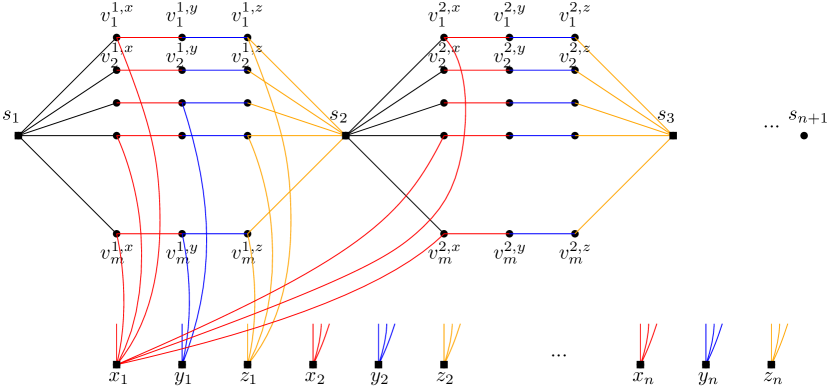
Figure 1: The graph ${\bar{G}}=({\bar{V}},{\bar{E}})$ used for the inapproximability and hardness proofs for $\mathsf{DDT}$ and $\mathsf{DDC}$. The inner edges have length $0$, and the outer edges have length $M$. Each square node represents a drone’s initial location. Each colored (red, blue, and orange) path represents a set of edges that can be visited by the same agent which is initially located at a location in $\{x_{i},y_{i},z_{i}\mid i\in[n]\}$. For each $i\in[n]$, there is an additional agent that is initially located at $s_{i}$ and which can visit edges $\{\{s_{i},v^{i,x}_{x}\}\mid j\in[m]\}$.

Now we define the set of agents. We have $4n$ agents with unit speed and unit energy consumption rate. Their initial locations are $\{x_{i},y_{i},z_{i},s_{i}\mid i\in[n]\}$. The agents with initial location in $\{x_{i},y_{i},z_{i}\mid i\in[n]\}$ are called element agents. For each $i\in[n]$, the node ranges and edge ranges of the agents with initial location with subscript $i$ are defined as follows:

• The agent located at $x_{i}$ has node range $\{x_{i},v^{i^{\prime},x}_{j},v^{i^{\prime},y}_{j}\mid i^{\prime}\in[n],j\in[m],f(j)=i\}$ and edge range $\{\{x_{i},v^{i^{\prime},x}_{j}\},\{v^{i^{\prime},x}_{j},v^{i^{\prime},y}_{j}\}\mid i^{\prime}\in[n],j\in[m],f(j)=i\}$.

• The agent located at $y_{i}$ has node range $\{y_{i},v^{i^{\prime},y}_{j},v^{i^{\prime},z}_{j}\mid i^{\prime}\in[n],j\in[m],g(j)=i\}$ and edge range $\{\{y_{i},v^{i^{\prime},y}_{j}\},\{v^{i^{\prime},y}_{j},v^{i^{\prime},z}_{j}\}\mid i^{\prime}\in[n],j\in[m],g(j)=i\}$.

• The agent located at $z_{i}$ has node range $\{z_{i},v^{i^{\prime},z}_{j},s_{i^{\prime}+1}\mid i^{\prime}\in[n],j\in[m],h(j)=i\}$ and edge range $\{\{z_{i},v^{i^{\prime},z}_{j}\},\{v^{i^{\prime},z}_{j},s_{i+1}\}\mid i^{\prime}\in[n],j\in[m],h(j)=i\}$.

• The agent located at $s_{i}$ has node range $\{s_{i},v^{i,x}_{j}\mid j\in[m]\}$ and edge range $\{\{s_{i},v^{i,x}_{j}\}\mid j\in[m]\}$.

We now show that the given instance of 3DM is a yes-instance if and only if the constructed base instance of $\mathsf{DDT}_{\mathsf{N}}$ has an optimal schedule with delivery time $M$. First, assume that the given instance of 3DM is a yes-instance, and let $\{t_{k_{1}},t_{k_{2}},\ldots,t_{k_{n}}\}\subseteq\mathcal{F}$ be a perfect matching. We let the package travel from $s_{1}$ to $s_{n+1}$ via the $n$ selection gadgets, using the path via nodes $v^{i,x}_{k_{i}},v^{i,y}_{k_{i}},v^{i,z}_{k_{i}}$ in selection gadget $i$, for $i\in[n]$. This path consists of $4n$ edges. Each of the $4n$ agents needs to carry the package on exactly one edge of this path. All the element agents reach the node where they pick up the package at time $M$. As all edges in the selection gadgets have length $0$, this shows that the package reaches $s_{n+1}$ at time $M$. It is clear that this solution is optimal because at least one element agent must take part in the delivery and cannot pick up the package before time $M$.

Now, assume that the base instance of $\mathsf{DDT}_{\mathsf{N}}$ admits a schedule with delivery time $M$. It is not hard to see that the schedule must be of the above format, using each agent on exactly one edge in one selection gadget. This is because it takes time $2M$ for an element agent to move from one selection gadget to another one via its initial location.

This shows that there is a schedule with delivery time $M$ if and only if the given instance of 3DM is a yes-instance. Furthermore, as any element agent needs time $M$ to reach a pick-up point in a selection gadget and time $2M$ to move to a different selection gadget (with or without the package), it is clear that the optimal schedule will have length at least $3M$ if the given instance of 3DM is a no-instance. This already shows that $\mathsf{DDT}_{\mathsf{N}}$ is $\mathit{NP}$-hard and does not admit a polynomial-time approximation algorithm with approximation ratio smaller than $3$ unless $P=\mathit{NP}$, but we can strengthen the inapproximability result by concatenating multiple copies of the base instance, as we show in the following theorem.

Theorem 3.1.

For any constant $\epsilon>0$, it is $\mathit{NP}$-hard to approximate $\mathsf{DDT}_{\mathsf{N}}$ (or $\mathsf{DDT}_{\mathsf{E}}$) within a factor of $O(\min\{n^{1-\epsilon},k^{1-\epsilon}\})$ even if all agents have the same speed.

Proof.

Consider the base instance $\bar{G}$ constructed from an instance $I$ of 3DM with $|X|=|Y|=|Z|=n$ and $|\mathcal{F}|=m$. To obtain a stronger inapproximability result for $\mathsf{DDT}_{\mathsf{N}}$, we concatenate $q$ copies of $\bar{G}$, for a suitable choice of $q$ (polynomial in $n$ and $m$). The node $s_{n+1}$ of each copy of $\bar{G}$ (except the last) is identified with the node $s_{1}$ of the next copy of $\bar{G}$. The package is initially located at the node $s_{1}$ of the first copy and needs to be delivered to node $s_{n+1}$ of the last copy. We call the initial location of the package $s$ (the node $s_{1}$ of the first copy) and the target location $y$ (the node $s_{n+1}$ of the last copy). The resulting instance of $\mathsf{DDT}_{\mathsf{N}}$ has $N=(4n+3mn)q+1$ nodes and $k=4nq$ agents. Let $G=(V,E)$ denote the graph of the resulting instance.

If the instance $I$ of 3DM admits a perfect matching, then there is an optimal schedule for the constructed instance of $\mathsf{DDT}_{\mathsf{N}}$ that has delivery time $M$: The element agents in all copies of $\bar{G}$ reach the node at which they pick up the package at time $M$. Otherwise, the best schedule for the constructed instance of $\mathsf{DDT}_{\mathsf{N}}$ has delivery time at least $M+q\cdot 2M=(1+2q)M$: It takes time $M$ for the first element agent to reach the location where it pick up the package; furthermore, in each of the $q$ copies of $\bar{G}$, at least one agent will have to carry the package over edges in two different selection gadgets, adding $2M$ to the delivery time. This shows that it is $\mathit{NP}$-hard to obtain an approximation ratio of at most $2q$.

We choose $q=(4n+3mn)^{c}$ for an arbitrarily large constant $c$. Then the constructed instance of $\mathsf{DDT}_{\mathsf{N}}$ has $N=(4n+3mn)q+1=(4n+3mn)^{c+1}+1$ nodes and $k=4nq=4n(4n+3mn)^{c}$ agents. As $q=(4n+3m)^{c}=(N-1)^{c/(c+1)}=\Omega(N^{1-1/(c+1)})$, this shows that there is no $O(N^{1-\epsilon})$-approximation algorithm unless $P=\mathit{NP}$. As $q=(4n+3m)^{c}\geq k^{c/(c+1)}=k^{1-1/(c+1)}$, there is also no $O(k^{1-\epsilon})$-approximation algorithm unless $P=\mathit{NP}$. ∎

To show $\mathit{NP}$-hardness for $\mathsf{DDC}$, we adapt the base instance by numbering the columns of the selection gadgets to which outer edges are attached from $1$ to $3n$ (from left to right) and letting the outer edges attached to column $i$ have length $2^{3n+1-i}$. If the given instance of 3DM is a yes-instance, exactly one outer edge attached to each column will be used, for a total energy consumption of $2^{3n+1}-2$. Otherwise, some column will be the first column in which an outer edge is used twice, and the total energy consumption will be at least $2^{3n+1}$.

Theorem 3.2.

The problems $\mathsf{DDC}_{\mathsf{N}}$ (and $\mathsf{DDC}_{\mathsf{E}}$) are $\mathit{NP}$-hard even if all agents have the same energy consumption.

Proof.

To prove the $\mathit{NP}$-hardness of $\mathsf{DDC}_{\mathsf{N}}$, we construct the graph $G=(V,E)$ from the base instance $\bar{G}$ by changing the lengths of the outer edges: For every $i\in[n]$ and $j\in[m]$, we let the outer edges $(x_{f(j)},v^{i,x}_{j})$, $(y_{g(j)},v^{i,y}_{j})$ and $(z_{h(j)},v^{i,z}_{j})$ have lengths $2^{3n+1-3(i-1)-1}$, $2^{3n+1-3(i-1)-2}$ and $2^{3n+1-3(i-1)-3}$, respectively. Intuitively, there are $3n$ columns of vertices in selection gadgets to which outer edges are attached (cf. Figure 1), and the lengths of the outer edges are powers of two that decrease column by column. The outer edges attached to the leftmost column (closest to $s_{1}$) have length $2^{3n}$, and those attached to the rightmost column (closest to $s_{n+1}$) have length $2$. The outer edges attached to the $k$-th column, $1\leq k\leq 3n$, have length $2^{3n+1-k}$.

If the instance of 3DM admits a perfect matching, then there is a schedule for the constructed instance of $\mathsf{DDC}_{\mathsf{N}}$ in which every agent carries the package over exactly one edge of a path in exactly one selection gadget. That schedule has total energy consumption $2^{3n}+2^{3n-1}+\cdots+2=2^{3n+1}-2$. Otherwise, at least one agent must carry the package over edges in at least two different selection gadgets. Assume that the first agent who does this picks up the package in column $k$. Then that agent will have energy consumption at least $2\cdot 2^{3n+1-k}$ because it needs to go back to its initial location after picking up the package. The previously used agents (who brought the package from $s_{1}$ to a node in column $k$) have energy consumption at least $2^{3n+1-1}+2^{3n+1-2}+\cdots+2^{3n+1-(k-1)}$. The total energy consumption is at least $\left(\sum_{t=1}^{k-1}2^{3n+1-t}\right)+2\cdot 3^{3n+1-k}=2^{3n+1}$. We conclude that there is a schedule with total energy consumption at most $2^{3n+1}-2$ if and only if the instance of 3DM is a yes-instance. ∎

Finally, for the problem variants without initial positions, we observe that the base instance admits a delivery schedule with delivery time $0$ and energy consumption $0$ if and only if the given instance of 3DM is a yes-instance. This shows that there cannot be any polynomial-time approximation algorithm for any of the $\mathsf{DDT}$ and $\mathsf{DDC}$ problem variants without initial positions.

Theorem 3.3.

For $\mathsf{DDT}_{\mathsf{N}}$ (or $\mathsf{DDT}_{\mathsf{E}}$) without initial positions, it is $\mathit{NP}$-hard to distinguish between instances with delivery time $0$ and instances with delivery time greater than $0$, even if all agents have the same speed. Therefore, there is no polynomial-time approximation algorithm for these problems (with any finite ratio), unless $P=\mathit{NP}$.

Proof.

For $\mathsf{DDT}_{\mathsf{N}}$ without initial positions, consider the base instance. If the given instance of 3DM is a yes-instance, there is a schedule in which the package travels along a path of $4n$ edges, these edges have length $0$, and each agent needs to carry the package over exactly one of these $4n$ edges. Hence, we can place each agent at the start of the edge over which it must carry the package, and the package can be delivered in time $0$. If the instance of 3DM is a no-instance, at least one element agent will have to carry the package on edges in two different selection gadgets, and that agent will require time $2M$ to travel to the second selection gadget. Thus, the delivery time will be at least $2M$. ∎

Theorem 3.4.

For $\mathsf{DDC}_{\mathsf{N}}$ (or $\mathsf{DDC}_{\mathsf{E}}$) without initial positions, it is $\mathit{NP}$-hard to distinguish between instances with energy consumption $0$ and instances with energy consumption greater than $0$, even if all agents have the same energy consumption rate. Therefore, there is no polynomial-time approximation algorithm for these problems (with any finite ratio), unless $P=\mathit{NP}$.

Proof.

We again use the base instance, and the argument is analogous to the proof of Theorem 3.3: If the instance of 3DM is a yes-instance, we can place each agent at the start of the edge over which it needs to carry the package, and the agent can carry the package over that edge with energy consumption $0$. Otherwise, at least one agent will have to travel between two different selection gadgets, consuming energy $2M$. ∎

Remark.

The results of Theorems 3.3 and 3.4 arise because we allow zero-length edges and it is $\mathit{NP}$-hard to decide whether an optimal solution with objective value $0$ exists. If we were to require strictly positive edge lengths, it would be possible to obtain approximation algorithms with ratios that depend on the ratio of maximum to minimum edge length.

4 Approximation algorithm for the $\mathsf{DDT}$ problem

First, we can show that an approach based on Dijkstra’s algorithm with time-dependent edge transit times (similar to [CEP21]) yields an optimal algorithm for the variant of $\mathsf{DDT}_{\mathsf{N}}$ where the solution can use an arbitrary number of copies of each agent (each copy of agent $a\in A$ has the same initial location $p_{a}$).

We start by introducing some notation used in the algorithm. For any edge $\{u,v\}\in E_{a}$ for some $a\in A$, we denote by $\mathsf{eT}_{a}(v,u\prec v)$ the earliest time for the package to arrive at $v$ if the package is carried over the edge $\{u,v\}$ by a copy of agent $a$. In addition, we use $\mathsf{eT}(v,u\prec v)$ to denote the earliest time for the package to arrive at node $v$ if the package is carried over the edge $\{u,v\}$ by some agent, i.e., $\mathsf{eT}(v,u\prec v)=\min\{\mathsf{eT}_{a}(v,u\prec v)\mid\{u,v\}\in E_{a},a\in A\}$. For every $v\in V$, we use $\mathsf{eT}(v)$ to denote the earliest arrival time for the package at node $v$, i.e., $\mathsf{eT}(v)=\min\{\mathsf{eT}(v,u\prec v)\mid\{u,v\}\in E\}$. Note that the package is initially at location $s$ at time $0$, i.e., $\mathsf{eT}(s)=0$. Given a node $v$, we denote by $\mathcal{S}(v)$ the schedule for carrying the package from $s$ to $v$, i.e., $\mathcal{S}(v)=\{(a_{1},s,u_{1}),(a_{2},u_{1},u_{2}),\ldots,(a_{h},u_{h-1},v)\}$.

Data: Graph $G=(V,E,\ell)$; package source node $s$ and target node $y$; agent $a$ with velocity $v_{a}$ and initial location $p_{a}$ for $a\in A$

Result: earliest arrival time for package at target location $y$, i.e., $\mathsf{eT}(y)$

1 begin

2      compute $\mathsf{dist}_{a}(p_{a},v)$ for $a\in A$ and $v\in V_{a}$

3      $\mathsf{eT}(s)\leftarrow 0$

4      $\mathsf{eT}(v)\leftarrow\infty$ for all $v\in V\setminus\{s\}$

5      $L(v)\leftarrow\emptyset$ for all $v\in V$ // agent bringing the package to $v$

6      

7      $\mathsf{proc}(v)\leftarrow 0$ for all $v\in V$ // all nodes $v$ are unprocessed

8      

9      $\mathsf{prev}(v)\leftarrow\emptyset$ for all $v\in V$ // previous node on optimal package path to $v$

10      

11      $Q\leftarrow\{s\}$ // priority queue of pending nodes

12      

13      while $Q\neq\emptyset$ do

14            

15            $u\leftarrow\arg\min\{\mathsf{eT}(v)\mid v\in Q\}$ // node with minimum arrival time in $Q$

16            

17            $Q\leftarrow Q\setminus\{u\}$ and $\mathsf{proc}(u)\leftarrow 1$

18            if $u=y$ then

19                   break

20             end if

21            

22            $t\leftarrow\mathsf{eT}(u)$ // arrival time when package reaches $u$

23            

24            for neighbors $v$ of $u$ with $\mathsf{proc}(v)=0$ and $A(u,v)\neq\emptyset$ do

25                   $\{\mathsf{eT}(v,u\prec v),L(v,u\prec v)\}\leftarrow$ NeiDelivery$(u,v,t)$

26                  if $\mathsf{eT}(v,u\prec v)<\mathsf{eT}(v)$ then

27                         $\mathsf{eT}(v)\leftarrow\mathsf{eT}(v,u\prec v)$

28                        $L(v)\leftarrow L(v,u\prec v)$

29                        $\mathsf{prev}(v)\leftarrow\{u\}$

30                        if $v\notin Q$ then

31                               $Q\leftarrow Q\cup\{v\}$ with earliest arrival time $\mathsf{eT}(v)$

32                         end if

33                        

34                   end if

35                  

36             end for

37            

38       end while

39      return $\mathsf{eT}(y)$

40 end

41

Algorithm 1 Algorithm for $\mathsf{DDT}$

Our algorithm adapts the approach of a time-dependent Dijkstra’s algorithm [BGM18, CEP21]. Algorithm 1 shows the pseudo-code. For each node $v\in V$, we maintain a value $\mathsf{eT}(v)$ that represents the current upper bound on the earliest time when the package can reach $v$ (line 3–4). Initially, we set the earliest arrival time for $s$ to $0$ and for all other nodes to $\infty$. We maintain a priority queue $Q$ of nodes $v$ with finite $\mathsf{eT}(v)$ value that have not been processed yet (line 8). In each iteration of the while-loop, we process a node $u$ in $Q$ having the earliest arrival time (line 10), where $u=s$ in the first iteration. For each unprocessed neighbor node $v$ of $u$, we calculate the earliest arrival time $\mathsf{eT}(v,u\prec v)$ at node $v$ if the package is carried over the edge between $u$ and $v$ by some agent (and we store the identity of that agent in $L(v,u\prec v)$), by calling the subroutine NeiDelivery$(u,v,t)$ (Algorithm 2). If this earliest arrival time is smaller than $\mathsf{eT}(v)$, then $\mathsf{eT}(v)$ is updated and $v$ is inserted into $Q$ (if it is not yet in $Q$) or its priority reduced to the new value of $\mathsf{eT}(v)$. The algorithm terminates and returns the value $\mathsf{eT}(y)$ when the node being processed is $y$ (line 12). The schedule $\mathcal{S}=\mathcal{S}(y)$ can be constructed in a backward manner because we store for each node $v$ the involved agent $L(v)$ and its predecessor node $\mathsf{prev}(v)$ (line 20 and 21).

To compute $\mathsf{eT}(v,u\prec v)$ in line 17 of Algorithm 1, we call NeiDelivery$(u,v,t)$ (Algorithm 2): That subroutine calculates for each agent $a\in A$ with $\{u,v\}\in E_{a}$, i.e., for all $a\in A(u,v)$, the time when the package reaches $v$ if that agent picks it up at $u$ and carries it over $\{u,v\}$ to $v$. The earliest arrival time at $v$ via the edge $\{u,v\}$ is returned as $\mathsf{eT}(v,u\prec v)$, and the agent $a^{*}$ achieving that arrival time is returned as $L(v,u\prec v)$.

Data: Edge $\{u,v\}$, arrival time for node $u$ $\mathsf{eT}(u)=t$, agents $A(u,v)$

Result: $\mathsf{eT}(v,u\prec v)$

1

2for $a\in A(u,v)$ do

3       $\mathsf{eT}_{a}(v,u\prec v)=\max\{t,\frac{\mathsf{dist}_{a}(p_{a},u)}{v_{a}}\}+\frac{\ell{(u,v)}}{v_{a}}$

4 end for

5

6$a^{*}=\arg\min\{\mathsf{eT}_{a}(v,u\prec v)\mid a\in A(u,v)\}$;

7$\mathsf{eT}(v,u\prec v)\leftarrow\mathsf{eT}_{a^{*}}(v,u\prec v)$

8$L(v,u\prec v)\leftarrow a^{*}$

return $\mathsf{eT}(v,u\prec v)$ and $L(v,u\prec v)$

Algorithm 2 Algorithm NeiDelivery$(u,v,t)$ for $\mathsf{DDT}_{\mathsf{N}}$

Lemma 4.1.

The following statements hold for the schedule found by Algorithm 1.

1. It may happen that an agent picks up and drops off the package more than once. Each time an agent $a$ carries the package over a path of consecutive edges, a copy of the agent starts at $p_{a}$, travels to the start node $u$ of the path, picks up the package at time $\max\{\mathsf{eT}(u),\frac{\mathsf{dist}_{a}(p_{a},u)}{v_{a}}\}$, and then carries the package over the edges of the path.

2. The package is carried to each node $v\in V$ at most once, and thus the schedule carries the package over at most $|V|-1$ edges.

Proof.

For statement (i), note that NeiDelivery$(u,v,t)$ (Algorithm 2) does not take into account whether an agent in $A(u,v)$ has already been involved in the trips that bring the package to $u$ at time $\mathsf{eT}(u)=t$ or not. Thus, it may select an agent again, and so agents may be involved in the schedule more than once, which means that a fresh copy of the agent is used each time the agent is involved. If an agent $a$ is used on two consecutive edges, then it can continue to carry the package over the second edge after it arrives at the endpoint of the first edge, and we do not need to use a fresh copy of the agent for the second edge.

According to lines 10–11 of Algorithm 1, the node $u$ being processed is removed from $Q$ and never enters $Q$ again (because $\mathsf{proc}(u)$ is set to 1 in line 11, and only nodes with $\mathsf{proc}(u)=0$ can be entered into $Q$ due to the condition in line 16). The node $u$ can become a predecessor (stored in $\mathsf{prev}(v)$) of another node $v$ only at the time when $u$ is being processed and the node $v$ has not yet been processed. Therefore, the resulting schedule for the delivery of the package visits each node at most once. This shows statement (ii). ∎

Lemma 4.2.

There is an algorithm that computes an optimal schedule in time $O(k(m+n\log n))$ for $\mathsf{DDT}_{\mathsf{N}}$ under the assumption that an arbitrary number of copies of each agent can be used. The package gets delivered from $s$ to $y$ along a simple path with at most $|V|-1$ edges.

Proof.

We claim that the arrival time $\mathsf{eT}(u)$ for each node $u$ is minimum by the time $u$ gets processed. Obviously, the first processed node $s$ has arrival time $\mathsf{eT}(s)=0$. Whenever a node $u$ is processed, the earliest arrival time for each unprocessed neighbor is updated (line 19 of Algorithm 1) if the package can reach that neighbor earlier via node $u$ (line 4 in Algorithm 2 identifies the agent $a^{*}$ that can bring the package from $u$ to the neighbor the fastest). At the time when a node $u$ is removed from the priority queue $Q$ and starts to be processed, all nodes $v$ with $\mathsf{eT}(v)<\mathsf{eT}(u)$ have already been processed, and so its value $\mathsf{eT}(u)$ must be equal to the earliest time when the package can reach $u$. The algorithm terminates when $y$ is removed from $Q$.

In lines 19–21 of Algorithm 1, we update the arrival time $\mathsf{eT}(v)$ and the agent $L(v)$ as well as the predecessor node $\mathsf{prev}(v)$ without explicitly maintaining the schedules $\mathcal{S}(v)$. The schedule $\mathcal{S}(v)$ can be retraced from $L(\cdot)$ and $\mathsf{prev}(\cdot)$ since the schedule found for $\mathsf{eT}(v)$ visits each node in $V$ at most once, cf. Lemma 4.1. This also shows that the package gets delivered from $s$ to $y$ along a simple path (with at most $|V|-1$ edges) in $G$.

We can analyze the running-time of Algorithm 1 as follows. The distances $\mathsf{dist}_{a}(p_{a},v)$ can be pre-computed by running Dijkstra’s algorithm with Fibonacci heaps in time $O(m+n\log n)$ [CLRS22] for each agent $a$ with source node $p_{a}$ in the graph $G_{a}$, taking total time $O(k(m+n\log n))$ (line 2). Selecting and removing a minimum element from the priority queue $Q$ in lines 10–11 takes time $O(\log n)$. At most $n$ nodes will be added into $Q$ (and later removed from $Q$), so the running time for inserting and removing elements from $Q$ is $O(n\log n)$. For each processed node $u$, we compute the value $\mathsf{eT}(v,u\prec v)$ for each unprocessed adjacent node $v$ with $A(u,v)\neq\emptyset$ in time $O(|A(u,v)|)$. Overall we get a running time of $O(k(m+n\log n)+n\log n+km)=O(k(m+n\log n))$. ∎

If the algorithm uses an agent $a$ on consecutive edges of the package delivery path, this can be seen as a single trip by agent $a$. If, however, the algorithm uses the same agent $a$ on edges that are not consecutive, then this corresponds to using different copies of agent $a$. This is because the algorithm assumes that $a$ can always travel from its initial location to the node where it picks up the package, which may be a shorter trip than traveling from the agent’s previous drop-off location to the pick-up node. Hence, the delivery schedule produced by the algorithm is guaranteed to be feasible only if we have arbitrarily many copies of each agent.

Next, we can show how to convert the delivery schedule $\mathcal{S}$ with delivery time $\mathcal{T}$ produced by the algorithm of Lemma 4.2 into a schedule that is feasible with a single copy per agent, and we bound the resulting increase in the delivery time $\mathcal{T}$ to obtain an approximation algorithm for $\mathsf{DDT}_{\mathsf{N}}$. The conversion consists of the repeated application of modification steps. Each step considers the first agent $a$ that is used at least twice. Let $a$ pick up the package at $u_{i-1}$ in its first trip and carry it from $u_{j-1}$ to $u_{j}$ in its last trip. We then modify the schedule so that $a$ picks up the package at $u_{i-1}$ and carries it all the way to $u_{j}$ along a shortest path in $G_{a}$. We have $\frac{1}{v_{a}}\mathsf{dist}_{a}(p_{a},u_{i-1})\leq\mathcal{T}$ and $\frac{1}{v_{a}}(\mathsf{dist}_{a}(p_{a},u_{j-1})+\mathsf{dist}_{a}(u_{j-1},u_{j}))\leq\mathcal{T}$. By the triangle inequality, $\mathsf{dist}_{a}(u_{i-1},u_{j})\leq\mathsf{dist}_{a}(u_{i-1},p_{a})+\mathsf{dist}_{a}(p_{a},u_{j-1})+\mathsf{dist}_{a}(u_{j-1},u_{j})$. Hence, agent $a$ needs time at most $2\mathcal{T}$ to carry the package from $u_{i-1}$ to $u_{j}$, and so the delivery time increases by at most $2\mathcal{T}$. Furthermore, we can bound the number of modification steps by $\min\{\frac{n-1}{3},k-1\}$.

Theorem 4.3.

There is a $\min\{2n/3+1/3,2k-1\}$-approximation algorithm for $\mathsf{DDT}_{\mathsf{N}}$.

Proof.

Based on the solution $\mathcal{S}(y)$ obtained by the algorithm of Lemma 4.2, we create a feasible solution $\mathcal{S}^{\prime}(y)$ for $\mathsf{DDT}_{\mathsf{N}}$ by modifying the schedule until each agent is involved in the delivery at most once. Initially, let $\mathcal{S}^{\prime}(y)=\mathcal{S}(y)$. Consider the first agent $a$ in $\mathcal{S}^{\prime}(y)$ that is involved in the delivery at least twice. Let $a$ be involved for the first time as the $i$-th agent and for the last time as the $j$-th agent. Then $a$ carries the package from node $u_{i-1}$ to node $u_{i}$ during its first involvement and from node $u_{j-1}$ to node $u_{j}$ during its last involvement in $\mathcal{S}^{\prime}(y)$, and at least one other agent is involved in carrying the package from $u_{i}$ to $u_{j-1}$. We modify the schedule and use agent $a$ to carry the package from $u_{i-1}$ to $u_{j}$ along a shortest path in $G_{a}$ and remove the trips made by the $(i+1)$-th agent to the $(j-1)$-th agent. If the package arrives at $u_{j}$ later in the resulting schedule, the times of all subsequent trips are delayed accordingly. Replace $\mathcal{S}^{\prime}(y)$ by the new schedule, and repeat this operation as long as there exists an agent that is involved in the delivery at least twice.

Note that the schedule $\mathcal{S}(y)$ transports the package over a path $P$ consisting of at most $n-1$ edges. A modification step that lets $a$ carry the package from $u_{i-1}$ to $u_{j}$ directly can be charged to three edges of $P$ that are not charged by any other modification step: An edge on $P$ between $u_{i-1}$ and $u_{i}$, one between $u_{i}$ and $u_{j-1}$, and one between $u_{j-1}$ and $u_{j}$. Therefore, there are at most $(n-1)/3$ modification steps. Similarly, the agent $a$ for which a modification step is carried out will not be involved in another modification step, and modification steps can only be necessary if there are still at least two agents for which no modification step has been carried out so far. Therefore, the number of modification steps can also be bounded by $k-1$. Thus, to obtain the final $S^{\prime}(y)$, we need to modify the schedule at most $\min\{(n-1)/3,k-1\}$ times.

Next, we bound the delivery time of the constructed schedule $\mathcal{S}^{\prime}(y)$. We claim that each modification step increases the delivery time of the package by at most $2\mathsf{eT}(y)$. Consider a modification step that lets agent $a$ carry the package from $u_{i-1}$ to $u_{j}$. Considering the original schedule $\mathcal{S}(y)$, we observe:

$$\mathsf{eT}(u_{i})\geq\frac{\mathsf{dist}_{a}(p_{a},u_{i-1})}{v_{a}}+\frac{\mathsf{dist}_{a}(u_{i-1},u_{i})}{v_{a}}$$

$$\mathsf{eT}(u_{j})\geq\frac{\mathsf{dist}_{a}(p_{a},u_{j-1})}{v_{a}}+\frac{\mathsf{dist}_{a}(u_{j-1},u_{j})}{v_{a}}$$

By the triangle inequality, we have $\mathsf{dist}_{a}(u_{i-1},u_{j})\leq\mathsf{dist}_{a}(u_{i-1},p_{a})+\mathsf{dist}_{a}(p_{a},u_{j-1})+\mathsf{dist}_{a}(u_{j-1},u_{j})$ and hence

$$\frac{\mathsf{dist}_{a}(u_{i-1},u_{j})}{v_{a}} \leq\frac{\mathsf{dist}_{a}(u_{i-1},p_{a})}{v_{a}}+\frac{\mathsf{dist}_{a}(p_{a},u_{j-1})}{v_{a}}+\frac{\mathsf{dist}_{a}(u_{j-1},u_{j})}{v_{a}}$$ (1)

$$\leq\mathsf{eT}(u_{i})+\mathsf{eT}(u_{j})\leq 2\cdot\mathsf{eT}(y)$$ (2)

The time when $a$ picks up the package at node $u_{i-1}$ is unchanged by the modification, and the time for carrying the package from $u_{i-1}$ to $u_{j}$ is at most $2\cdot\mathsf{eT}(y)$ after the modification. Therefore, the time when the package reaches $u_{j}$, and hence the delivery time of the package at $y$, increases by at most $2\cdot\mathsf{eT}(y)$ in the modification, as claimed.

Since there are at most $\min\{(n-1)/3,k-1\}$ modification steps, we have

$$\mathsf{eT}^{\prime}(y)\leq\mathsf{eT}(y)+\min\{(n-1)/3,k-1\}\cdot 2\cdot\mathsf{eT}(y)=\min\{2n/3+1/3,2k-1\}\cdot\mathsf{eT}(y).$$

This completes the proof. ∎

To adapt the approach from $\mathsf{DDT}_{\mathsf{N}}$ to $\mathsf{DDT}_{\mathsf{E}}$, we can adapt the algorithm of Lemma 4.2 to edge handovers by using as a subroutine the FastLineDelivery$(u,v,t)$ method from [CEP21], which calculates in $O(k\log k)$ time an optimal delivery schedule using the agents in $A(u,v)$ to transport the package that arrives at $u$ at time $t$ from $u$ to $v$ over the edge $\{u,v\}$. When transforming the resulting package delivery schedule into one that uses each agent at most once, the number of modification steps can be bounded by $\min\{n-1,k-1\}$.

For $\mathsf{DDT}_{\mathsf{E}}$, we may need to choose a set of agents to collaborate on carrying the package over an edge $\{u,v\}$ since the package can be handed over at any point in the interior of the edge. Therefore, in line 17 of Algorithm 1 we now call as subroutine NeiDelivery$(u,v,t)$ instead of Algorithm 2 a subroutine that computes the fastest way for carrying the package from $u$ to $v$ over the edge $\{u,v\}$ assuming that the package has arrived at node $u$ at time $t$. This subproblem can be solved in $O(k\log k)$ time using the algorithm FastLineDelivery$(u,v,t)$ from [CEP21]. That algorithm can be applied in our setting with movement restrictions because it considers a single edge $\{u,v\}$. Only the agents in $A(u,v)$ are relevant for the solution, and all other agents can be ignored. We know for each agent in $A(u,v)$ the earliest time when it can reach $u$ and the earliest time when it can reach $v$, and so we can execute FastLineDelivery$(u,v,t)$ (together with its subroutines PreprocessSender and PreprocessReceiver) from [CEP21] in $O(k\log k)$ time.

Similar to Lemma 4.2, we thus get the following:

Lemma 4.4.

Algorithm 1 computes an optimal schedule for $\mathsf{DDT}_{\mathsf{E}}$ in time $O(k(m\log k+n\log n))$ under the assumption that an arbitrary number of copies of each agent can be used.

We note that the schedule produced for agents collaborating to transport the package over an edge $\{u,v\}$ by algorithm FastLineDelivery$(u,v,t)$ from [CEP21] has the property that the velocities of the agents used are strictly increasing. Therefore, each agent is used at most once on each edge of the path along which the package is delivered from $s$ to $y$. We can now show the following theorem:

Theorem 4.5.

There is a $\min\{2n-1,2k-1\}$-approximation algorithm for $\mathsf{DDT}_{\mathsf{E}}$.

Proof.

Similar to the proof of Theorem 4.3, we repeatedly modify the schedule $\mathcal{S}$ obtained by Algorithm 1 (using FastLineDelivery from [CEP21] as the NeiDelivery subroutine) for $\mathsf{DDT}_{\mathsf{E}}$ until each agent is involved at most once. The difference here is that every modification can only be charged to a single edge, not three edges. For example, if the modification operation is applied to an agent $a$ that carries the package on parts of consecutive edges $e_{1}$ and $e_{2}$, then the modification can only be charged to $e_{1}$, because another agent carrying the package on a later part of $e_{2}$ may be involved in another modification. Thus, the number of modification steps can only be bounded by $\min\{n-1,k-1\}$. By similar arguments as in the proof of Theorem 4.3, we get $\mathsf{eT}^{\prime}(y)\leq\min\{2n-1,2k-1\}\cdot\mathsf{eT}(y)$. ∎

5 Approximation algorithm for the $\mathsf{DDC}$ problem

By Lemma 2.2, handovers on interior points of edges are not needed for $\mathsf{DDC}$, so the results for $\mathsf{DDC}_{\mathsf{N}}$ that we present in this section automatically apply to $\mathsf{DDC}_{\mathsf{E}}$ as well. Therefore, we only consider $\mathsf{DDC}_{\mathsf{N}}$ in the proofs. We first give an algorithm that solves $\mathsf{DDC}_{\mathsf{N}}$ optimally if there is a sufficient number of copies of every agent.

Let an instance of $\mathsf{DDC}_{\mathsf{N}}$ be given by a graph $G=(V,E,\ell)$, package start node $s$ and destination node $y$, and a set $A$ of $k$ agents where $a=(p_{a},v_{a},w_{a},V_{a},E_{a})$ for $a\in A$. We create a directed graph $G^{\prime}$ in which a shortest path from $s^{\prime}$ to $y^{\prime}$ corresponds to an optimal delivery schedule. This approach is motivated by a method used by Bärtschi et al. [BCD⁺17]. We construct the directed edge-weighted graph $G^{\prime}=(V^{\prime},E^{\prime},\ell^{\prime})$ as follows:

• For each node $u\in V$ and each agent $a\in A$ with $u\in V_{a}$, create a node $u_{a}$ in $V^{\prime}$. In addition, add a node $s^{\prime}$ and a node $y^{\prime}$.

• For all $a\in A$ with $s\in V_{a}$, add an arc $(s^{\prime},s_{a})$ with $\ell^{\prime}{(s^{\prime},s_{a})}=w_{a}\cdot\mathsf{dist}_{a}(p_{a},s)$. For all $a\in A$ with $y\in V_{a}$, add an arc $(y_{a},y^{\prime})$ with $\ell^{\prime}{(y_{a},y^{\prime})}=0$.

• For $\{u,x\}\in E$, for each $a$ with $\{u,x\}\in E_{a}$, create two arcs $(u_{a},x_{a})$ and $(x_{a},u_{a})$ with $\ell^{\prime}{(x_{a},u_{a})}=\ell^{\prime}{(u_{a},x_{a})}=w_{a}\cdot\ell{(u,x)}$.

• For $u\in V$ and agents $a,\bar{a}\in A(u)$, create the following two arcs: $(u_{a},u_{\bar{a}})$ with $\ell^{\prime}{(u_{a},u_{\bar{a}})}=w_{\bar{a}}\cdot\mathsf{dist}_{\bar{a}}(p_{\bar{a}},u)$, and $(u_{\bar{a}},u_{a})$ with $\ell^{\prime}{(u_{\bar{a}},u_{a})}=w_{a}\cdot\mathsf{dist}_{a}(p_{a},u)$.

Intuitively, a node $u_{a}$ in $G^{\prime}$ represents the agent $a$ carrying the package at node $u$ in $G$. An arc $(u_{a},x_{a})$ represent the agent $a$ carrying the package over edge $\{u,x\}$ from $u$ to $x$. An arc $(u_{a},u_{\bar{a}})$ represents a copy of agent $\bar{a}$ traveling from $p_{\bar{a}}$ to $u$ and taking over the package from agent $a$ there. We can show that a shortest $s^{\prime}$-$y^{\prime}$ path in $G^{\prime}$ corresponds to an optimal schedule with multiple copies per agent.

Lemma 5.1.

An optimal schedule for $\mathsf{DDC}_{\mathsf{N}}$ (and $\mathsf{DDC}_{\mathsf{E}}$) can be computed in time $O(nk^{2}+n^{2}k)$ under the assumption that an arbitrary number of copies of each agent can be used.

Proof.

We claim that a shortest $s^{\prime}$-$y^{\prime}$ path in $G^{\prime}$ corresponds to an optimal delivery schedule. First, assume that an optimal delivery schedule $\mathcal{S}$ is

$$\{(a_{1},s,u_{1}),(a_{2},u_{1},u_{2}),\ldots,(a_{h},u_{h-1},y)\},$$

where it is possible that $a_{i}=a_{j}$ for $j>i+1$ because we allow copies of agents to be used. Then we can construct an $s^{\prime}$-$y^{\prime}$ path in $G^{\prime}$ whose length equals the total energy consumption of $\mathcal{S}$ as follows: Start with the arc $(s^{\prime},s_{a_{1}})$. Then use the arcs $(s_{a_{1}},z^{(1)}_{a_{1}}),\ldots,(z^{(g)}_{a_{1}},{u_{1}}_{a_{1}})$ corresponding to the path $s,z^{(1)},\ldots,z^{(g)},u_{1}$ (for some $g\geq 0$) along which agent $a_{1}$ carries the package from $s$ to $u_{1}$ in $\mathcal{S}$. Next, use the arc $({u_{1}}_{a_{1}},{u_{1}}_{a_{2}})$ representing the handover from $a_{1}$ to $a_{2}$ at $u_{1}$. Continue in this way until node $y_{a_{h}}$ is reached, and then follow the arc from there to $y^{\prime}$. Similarly, any $s^{\prime}$-$y^{\prime}$ path $P$ in $G^{\prime}$ can be translated into a delivery schedule in $G$ whose total energy consumption is equal to the length of $P$ in $G^{\prime}$.

Finally, let us consider the running-time of the algorithm. First, we compute $\mathsf{dist}_{a}(p_{a},v)$ for each agent $a$ and each node $v\in V$ by running Dijkstra’s algorithm with Fibonacci heaps [CLRS22] once in $G_{a}$ with source node $p_{a}$ for each $a\in A$, taking time $O(k(n\log n+m))=O(kn^{2})$. The graph $G^{\prime}$ has at most $n\cdot k+2\in O(nk)$ vertices and at most $2k+(n^{2}\cdot k+n\cdot k^{2})\in O(nk^{2}+n^{2}k)$ arcs. It can be constructed in $O(nk^{2}+n^{2}k)$ time as we have pre-computed the values $\mathsf{dist}_{a}(p_{a},v)$. We can compute the shortest $s^{\prime}$-$y^{\prime}$ path in $G^{\prime}$ in time $O(nk^{2}+n^{2}k+nk\log(nk))=O(nk^{2}+n^{2}k)$ time using Dijkstra’s algorithm. ∎

Theorem 5.2.

There is a 2-approximation algorithm for $\mathsf{DDC}_{\mathsf{N}}$ (and $\mathsf{DDC}_{\mathsf{E}}$).

Proof.

Let an instance of $\mathsf{DDC}_{\mathsf{N}}$ be given by a graph $G=(V,E,\ell)$, package start node $s$ and destination node $y$, and a set $A$ of $k$ agents where $a=(p_{a},v_{a},w_{a},V_{a},E_{a})$ for $a\in A$. Compute an optimal delivery schedule that may use multiple copies of agents using the algorithm of Lemma 5.1. Then we transform the schedule into one that uses each agent at most once as follows: Let $a$ be the first agent that is used more than once in the delivery schedule. Assume that $a$ carries the package from node $u$ to node $v$ during its first involvement in the delivery and from node $u^{\prime}$ to node $v^{\prime}$ during its last involvement in the delivery. The energy consumed by these two copies of agent $a$ is:

$$W_{a}=w_{a}(\mathsf{dist}_{a}(p_{a},u)+\mathsf{dist}_{a}(u,v)+\mathsf{dist}_{a}(p_{a},u^{\prime})+\mathsf{dist}_{a}(u^{\prime},v^{\prime}))$$

We modify the schedule and let agent $a$ pick up the package at $u$ and carry it along a shortest path in $G_{a}$ from $u$ to $v^{\prime}$. The trips in the original schedule that bring the package from $v$ to $u^{\prime}$ are removed. The new energy consumption by agent $a$ is $w_{a}(\mathsf{dist}_{a}(p_{a},u)+\mathsf{dist}_{a}(u,v^{\prime}))$. By the triangle inequality, $\mathsf{dist}_{a}(u,v^{\prime})\leq\mathsf{dist}_{a}(u,p_{a})+\mathsf{dist}_{a}(p_{a},u^{\prime})+\mathsf{dist}_{a}(u^{\prime},v^{\prime})$. Hence, the new energy consumption is bounded by $2W_{a}$. As long as there is an agent that is used more than once, we apply the same modification step to the first such agent. The procedure terminates after at most $k-1$ modification steps. During the execution of the procedure, the energy consumption of every agent at most doubles. Therefore, the total energy consumption of the resulting schedule for $\mathsf{DDC}_{\mathsf{N}}$ with a single copy of each agent is at most twice the total energy consumption of $\mathcal{S}$, which is a lower bound on the optimal energy consumption.

The algorithm of Lemma 5.1 takes $O(nk^{2}+n^{2}k)$ time, which dominates the time needed to carry out the modification steps. Thus, the overall running time is $O(nk^{2}+n^{2}k)$. ∎

6 Drone delivery on path and tree networks

6.1 Hardness of $\mathsf{DDT}$ on the path

Theorem 6.1.

$\mathsf{DDT}_{\mathsf{N}}$ and $\mathsf{DDT}_{\mathsf{E}}$ with initial positions are $\mathit{NP}$-complete if the given graph is a path.

Proof.

We give a reduction from the $\mathit{NP}$-complete Even-Odd Partition (EOP) problem [GJ79] that is defined as follows: Given a set of $2n$ positive integers $X=\{x_{1},x_{2},\ldots,x_{2n}\}$, is there a partition of $X$ into two subsets $X_{1}$ and $X_{2}$ such that $\sum_{x_{i}\in X_{1}}x_{i}=\sum_{x_{i}\in X_{2}}x_{i}$ and such that, for each $i\in 1,2,\ldots,n$, $X_{1}$ (and also $X_{2}$) contains exactly one element of $\{x_{2i-1},x_{2i}\}$?

Let an instance of EOP be given by $2n$ numbers $\{x_{1},x_{2},\ldots,x_{2n-1},x_{2n}\}$. Construct a path (see Figure 2) with set of nodes $\{s,b_{1},b_{2},\ldots,b_{2n},z,z^{\prime},c_{2n},c_{2n-1},\ldots,c_{1},y,u\}$ ordered from left to right. The length of each edge corresponds to the Euclidean distance between its endpoints. We let $z^{\prime}-z=b_{2i}-b_{2i-1}=1$, $c_{2i-1}-c_{2i}=1/2$, $z-b_{2n}=c_{2n}-z^{\prime}=y-c_{1}=L$, and $b_{2i+1}-b_{2i}=c_{2i}-c_{2i+1}=L$ for all $i\in[n-1]$ where $L=3Cn/2+7/4+1$. Furthermore, we let $b_{1}-s=S$, where $S>0$ is specified later. The node $u$ is placed so that $u-z=b_{1}-s+Cn+0.5$, where $C$ is a constant that we can set to $C=3$. There are $4n+3$ agents:

• Two agents $h_{1},h_{2}$: These agents have speed $1$. Agent $h_{1}$ is initially at node $s$ and can traverse the interval $[s,b_{1}]$. Agent $h_{2}$ is initially at node $u$ and can traverse the interval $[z,u]$.

• $2n$ agents $p_{1},p_{2},\ldots,p_{2n}$: These agents are initially at node $z$; each agent $p_{i}$ has speed $v_{p_{i}}=\frac{1}{C+x_{i}/M}$ where $M=\sum_{i\in[2n]}x_{i}$. Agents $p_{2i-1}$ and $p_{2i}$ for $i\in[n]$ can traverse the interval $[b_{2i-1},c_{2i-1}]$.

• $2n+1$ agents $f_{1},f_{2},\ldots,f_{2n},f_{2n+1}$: These agents have infinite speed. Each agent $f_{i}$ for $i<n$ is initially at node $b_{2i}$ and can traverse the interval $[b_{2i},b_{2i+1}]$; agent $f_{n}$ is initially at node $b_{2n}$ and can traverse the interval $[b_{2n},z]$; agent $f_{n+1}$ is initially at node $z^{\prime}$ and can traverse the interval $[z^{\prime},c_{2n}]$; each agent $f_{i}$ for $n+1<i\leq 2n$ is initially at node $c_{2(2n+1-i)+1}$ and can traverse the interval $[c_{2(2n+1-i)+1},c_{2(2n+1-i)}]$; agent $f_{2n+1}$ is initially at node $c_{1}$ and can traverse the interval $[c_{1},y]$.

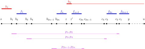
Figure 2: Instance of $\mathsf{DDT}_{\mathsf{N}}$ on a path

The goal is to deliver a package from $s$ to $y$ as quickly as possible. We claim that there is a schedule with delivery time at most $T=S+3Cn/2+7/4$ if and only if the original instance of EOP is a yes-instance.

First, assume that the instance of EOP is a yes-instance with partition $(X_{1},X_{2})$. Let $(P_{1},P_{2})$ be the corresponding partition of the set containing the $2n$ agents $p_{i}$. We construct a delivery schedule for the package as follows (the colors we mention refer to those shown in Figure 2). Until time $S=b_{1}-s$, the agent $h_{1}$ carries the package to $b_{1}$, and all agents $p_{i}$ pick a bold purple interval and arrive at its left endpoint. This is done in such a way that agent $p_{i}$ picks its left bold purple interval (the interval of length 1 at the left end of its range) if $p_{i}\in P_{1}$, and its right bold purple interval (the interval of length $\frac{1}{2}$ at the right end of its range) otherwise. To guarantee that any agent $p_{i}$ arrives at the left endpoint of its interval by time $S$, we set $S=\max_{i\in[n]}\frac{(n+1-i)(L+1)}{\min\{p_{2i-1},p_{2i}\}}$. Next, the package travels from $b_{1}$ to $z$ by always being alternatingly carried by an agent $p_{i}$ over a bold purple interval of length 1 and an infinite speed agent $f$ over a blue interval of length $L$. The package thus reaches $z$ at time $S+Cn+1/2$ (because $\sum_{x_{i}\in X_{1}}x_{i}/M=1/2$). As $u-z=S+Cn+1/2$, the agent $h_{2}$ arrives at $z$ at exactly the same time. Then, the agent $h_{2}$ carries the package from $z$ to $z^{\prime}$ in time $1$. After that, the package is alternatingly carried by an infinite speed agent and an agent $p_{i}$ until it reaches $y$, taking time $Cn/2+1/4$. The total delivery time is $S+Cn+1/2+1+Cn/2+1/4=S+3Cn/2+7/4=T$ as required.

Now consider the case that the original EOP instance is a no-instance. Assume that there exists a delivery schedule with delivery time $T=S+3Cn/2+7/4$. First, we claim that neither an agent $p_{i}$ nor the agent $h_{2}$ can carry the package over an interval of length $L$ (these are the intervals $[b_{2n},z]$, $[z^{\prime},c_{2n}]$, $[c_{1},y]$, and the intervals $[b_{2i},b_{2i+1}]$, $[c_{2i+1},c_{2i}]$ for any $i\in[n-1]$). Otherwise, the delivery time is larger than $S+L>S+3Cn/2+7/4$ because these agents have speed at most $1$ and these blue intervals have length $L=3Cn/2+7/4+1$. Therefore, it is clear that each of the $2n$ agents $p_{i}$ and the agent $h_{2}$ will carry the package over exactly one of the following $2n+1$ intervals: the interval $[b_{1},b_{2}]$, and the $2n$ intervals that lie between two consecutive blue intervals. Next, we claim that $h_{2}$ must carry the package over the interval $[z,z^{\prime}]$ with length $1$. Otherwise, $h_{2}$ would have to carry the package over an interval $[c_{2i},c_{2i-1}]$ with length $1/2$, and an agent $p_{i}$ with speed less than $1/C$ would have to carry the package through $[z,z^{\prime}]$ with length $1$ instead. Even if we assume that all agents $p_{i}$ have the faster speed $1/C$, the resulting schedule would have delivery time at least $S+nC+C+(n-1)C/2+1/2=S+3Cn/2+C/2+1/2$, which is larger than $T=S+3Cn/2+7/4$ as $C=3>5/2$.

This implies that agent $h_{2}$ carries the package over $[z,z^{\prime}]$ and, for each $i\in[n]$, one agent among $\{p_{2i-1},p_{2i}\}$ carries the package on a bold purple interval to the left of $z$ and the other agent carries the package on a bold purple interval to the right of $z^{\prime}$. Let the resulting partition of the agents $p_{i}$ be $(P_{1},P_{2})$, and let the corresponding partition of the original EOP instance be $(X_{1},X_{2})$. Suppose the package arrives at node $z$ at time $S+W$. Since the instance of EOP is a no-instance, either $W>Cn+1/2$ or $W<Cn+1/2$ holds. As the agents $p_{i}$ that carry the package to the left of $z$ take time $W$ in total, the agents $p_{i}$ that carry the package over intervals to the right of $z^{\prime}$ take time $\frac{2Cn+1-W}{2}$ in total. Consider the two cases:

• $W>Cn+1/2$. As agent $h_{2}$ carries the package from $z$ to $z^{\prime}$, the delivery time is $S+W+1+\frac{2Cn+1-W}{2}=S+Cn+W/2+3/2>S+3Cn/2+7/4=T$, a contradiction.

• $W<Cn+1/2$. As agent $h_{2}$ carries the package from $z$ to $z^{\prime}$, the package must wait at $z$ until time $S+Cn+1/2$ when $h_{2}$ reaches $z$. The delivery time is $S+Cn+1/2+1+\frac{2Cn+1-W}{2}=S+2Cn+2-W/2>S+2Cn+2-(Cn+1/2)/2=S+3Cn/2+7/4=T$, a contradiction.

Finally, we observe that in the constructed instance of $\mathsf{DDT}$, the availability of edge handovers has no impact on the existence of a schedule with delivery time $S+3Cn/2+7/4$. Therefore, the reduction establishes $\mathit{NP}$-hardness of both $\mathsf{DDT}_{\mathsf{N}}$ and $\mathsf{DDT}_{\mathsf{E}}$. ∎

6.2 Algorithms for drone delivery on a tree

In this section, we show that all variants of the drone delivery problem can be solved optimally in polynomial time if the graph is a tree and all agents have the same speed (for minimizing the delivery time) or the same energy consumption rate (for minimizing the total energy consumption). In fact, the algorithms extend to the case of general graphs if the subgraph $G_{a}=(V_{a},E_{a})$ of each agent is isometric, i.e., it satisfies the following condition: For any two nodes $u,v\in V_{a}$, the length of the shortest $u$-$v$ path in $G_{a}$ is equal to the length of the shortest $u$-$v$ path in $G$. If the given graph is a tree, the subgraph $G_{a}$ of every agent $a$ is necessarily isometric because we assume that $G_{a}$ is connected and there is a unique path between any two nodes in a tree.

If all agents have the same speed (for $\mathsf{DDT}$) or the same consumption rate (for $\mathsf{DDC}$), handovers at internal points of edges can never improve the objective value. Therefore, we only need to consider $\mathsf{DDT}_{\mathsf{N}}$ and $\mathsf{DDC}_{\mathsf{N}}$ in the following.

The crucial ingredient of our algorithms for the case of isometric subgraphs $G_{a}$ is:

Lemma 6.2.

Consider a delivery schedule $\mathcal{S}$ that may use an arbitrary number of copies of each agent. If the subgraph of each agent is isometric and all agents have the same speed (or the same energy consumption rate), then $\mathcal{S}$ can be transformed in time $O(k(m+n\log n))$ into a schedule in which each agent is used at most once without increasing the delivery time (or the energy consumption).

Proof.

Consider the first agent $a$ that is used at least twice in $\mathcal{S}$. Assume that it carries the package from $u_{i-1}$ to $u_{i}$ in its first trip and from $u_{j-1}$ to $u_{j}$ in its last trip. Change the schedule so that $a$ carries the package from $u_{i-1}$ to $u_{j}$, and discard the trips by agents $i+1,\ldots,j-1$. As $G_{a}$ is isometric, the agent $a$ carries the package from $u_{i-1}$ to $u_{j}$ along a shortest path in $G$, and hence neither the time (in case of equal speed) nor the energy consumption (in case of equal energy consumption rate) increase by this modification. Repeat the modification step until every agent is used at most once.

There are at most $k-1$ modification steps, and each of them can be implemented in $O(m+n\log n)$ time using Dijkstra’s algorithm with Fibonacci heaps [CLRS22]. ∎

Theorem 6.3.

$\mathsf{DDT}_{\mathsf{N}}$ (and $\mathsf{DDT}_{\mathsf{E}}$) can be solved optimally in time $O(k(n\log n+m))$ if all agents have the same speed and the subgraph of every agent is isometric.

Proof.

Compute an optimal delivery schedule that may use multiple copies of each agent using Lemma 4.2 and then apply Lemma 6.2. ∎

Theorem 6.4.

$\mathsf{DDC}_{\mathsf{N}}$ (and $\mathsf{DDC}_{\mathsf{E}}$) can be solved optimally in time $O(nk^{2}+n^{2}k)$ if all agents have the same speed and the subgraph of every agent is isometric.

Proof.

Compute an optimal delivery schedule that may use multiple copies of each agent using Lemma 5.1 and then apply Lemma 6.2. ∎

The problem variants without initial positions can also be solved optimally in polynomial time: We simply compute a shortest $s$-$y$-path $P$ and place on each edge $e$ of $P$ a copy of an arbitrary agent in $A(e)$ and then apply Lemma 6.2.

For the special case where $G$ is a tree, the running-time for $\mathsf{DDT}_{\mathsf{N}}$ can be improved to $O(kn)$ by using a simple algorithm that can even be implemented in a distributed way: The package acts as a magnet, and each agent moves towards the package until it meets the package and then follows it (or carries it) towards $y$ as long as its range allows. When several agents are at the same location as the package, the one whose range extends furthest towards $y$ carries the package.

For the case where the given graph $G$ is a tree, we first have the following observation:

Observation 6.5.

For any instance of the $\mathsf{DDT}$ or $\mathsf{DDC}$ problem on a tree, there is an optimal solution in which the package is carried along the unique simple path $\mathsf{Path}(s,y)$ between start node $s$ and destination node $y$.

Proof.

If the package was ever transported away from $\mathsf{Path}(s,y)$, it would have to be returned to $\mathsf{Path}(s,y)$ before moving closer to $y$ on $\mathsf{Path}(s,y)$, and this detour could be removed from the solution without increasing the delivery time or energy consumption. ∎

Lemma 6.6.

For any instance of $\mathsf{DDT}$ on a tree, if all agents have the same speed, we can find an optimal solution for both $\mathsf{DDT}_{\mathsf{N}}$ and $\mathsf{DDT}_{\mathsf{E}}$ with initial positions in time $O(kn)$. Furthermore, we can find an optimal solution for both $\mathsf{DDT}_{\mathsf{N}}$ and $\mathsf{DDT}_{\mathsf{E}}$ without initial positions in time $O(kn)$.

Proof.

Consider this algorithm for $\mathsf{DDT}_{\mathsf{N}}$ with initial positions:

• At any moment in time, starting at $t=0$, each agent $a$ moves from its initial location $p_{a}$ towards the current location of the package; it only stops moving when it hits an endpoint of its node range.

• At each moment in time $t$ when there is a set of agents that is at the same location as the package and at least one of them can carry the package in the direction of $y$, let $D(t)$ be the set of agents that can carry the package further in the direction of $y$. Let the agent $a$ in $D(t)$ that contains the node $b(a)$ closest to $y$ in $V_{a}\cap V(\mathsf{Path}(s,y))$ take the package and carry it towards $b(a)$ until it either reaches $b(a)$ or the package can be transferred at a node to another agent $a^{\prime}$ whose node $b(a^{\prime})$ is closer to $y$ than $b(a)$.

In this algorithm, the package acts like a magnet and all agents act like pieces of metal that are attracted by the magnet. When the package is “touched” by an agent, it moves with unit speed in this agent’s edge-range in the package path until it is handed over to another agent, which happens when it is not possible for the agent to carry the package further or if there is another agent at the location of the package whose edge range is larger. We remark that this algorithm could be implemented in a distributed manner as each agent only needs to know the current location of the package to determine its movement.

We denote the nodes where the package is picked up by the first agent or handed over from one agent to another agent or delivered to $y$ by $H=\{u_{1},u_{2},...,u_{h}\}$ with $|H|=h$ in order from $u_{1}=s$ to $u_{h}=y$. Obviously, the package is handed to a different agent at each handover node. Let agent $i$ be the agent that carries the package from $u_{i-1}$ to $u_{i}$, for $2\leq i\leq h$. Next, we show that the package is delivered to $u_{h}=y$ with minimum delivery time.

We can prove that the package reaches each node of $H$ as early as possible by induction. Let $P(u_{i})$ be the statement that the package reaches $u_{i}$ as early as possible. The base case $P(u_{1})$ is obvious, as the package is at $u_{1}=s$ at time $0$. Next, we show that for every node $u_{i}\in H$ with $i<h$, if $P(u_{i})$ holds, then $P(u_{i+1})$ also holds. Note that the package reaches $u_{i+1}$ at the time that is equal to the maximum of the package’s arrival time at node $u_{i}$ and agent $i+1$’s arrival time at $u_{i}$, plus the travel time from $u_{i}$ to $u_{i+1}$. By the inductive hypothesis, the package is carried to $u_{i}$ with minimum arrival time, and the travel time from $u_{i}$ to $u_{i+1}$ is fixed because the speed of all agents is the same. So we only need to show that the package is handed at $u_{i}$ to an agent that reaches $u_{i}$ as early as possible among all agents that can carry the package from $u_{i}$ closer towards $y$.

Assume that $a^{*}$ is the agent that can reach $u_{i}$ as early as possible and that can carry the package closer towards $y$. In the algorithm, agent $a^{*}$ first moves from its initial location to the closest node $v$ on $\mathsf{Path}(s,y)$. At the time when $a^{*}$ reaches $v$, there are two possibilities: If the package is already closer to $y$ than $v$, then $a^{*}$ will chase the package and reach node $u_{i}$ as early as possible. If the package is further from $y$ than $v$, then $a^{*}$ will first move towards the package until it is in the same location and then travel along with the package at the same speed until the package reaches $u_{i}$. Thus, $a^{*}$ is guaranteed to reach $u_{i}$ by the time when the package reaches $u_{i}$ or as early as possible afterwards. Thus, $P(u_{i+1})$ holds as well.

Note that the proof for $\mathsf{DDT}_{\mathsf{E}}$ is the same, because handovers in interior points of edges cannot reduce the delivery time if all agents have the same speed.

For the setting without initial locations, we choose for each agent $a\in A$ with $V(\mathsf{Path}(s,y))\cap V_{a}\neq\emptyset$ as initial location $p_{a}$ the node on $V(\mathsf{Path}(s,y))\cap V_{a}$ that is closest to $s$. The remaining agents (if any) do not participate in the delivery of the package, and their initial locations can be chosen arbitrarily. It is easy to see that the delivery time is then equal to the length of $\mathsf{Path}(s,y)$ divided by the speed of the agents, which is clearly optimal.

The algorithms for all problem variants can be implemented in $O(kn)$ time using standard techniques. In particular, for each agent $a\in A$, we can in $O(n)$ time determine for each node on $\mathsf{Path}(s,y)$ the earliest time when $a$ can reach that node. Whenever the package reaches a node $v$ on $\mathsf{Path}(s,y)$, we can then in $O(k)$ time identify the earliest agent that can carry the package from $v$ to the next node in the path. ∎

Furthermore, we have:

Corollary 6.7.

We can determine an optimal solution for both $\mathsf{DDC}_{\mathsf{N}}$ and $\mathsf{DDC}_{\mathsf{E}}$ without initial positions in time $O(kn)$ on a tree if all agents have the same consumption rate.

Proof.

Since the package is delivered following a fixed path, the energy consumption of the optimal solution for both $\mathsf{DDC}_{\mathsf{N}}$ and $\mathsf{DDC}_{\mathsf{E}}$ without initial locations is simply equal to the total energy consumption of carrying the package over the fixed path, i.e., $\frac{\sum_{e\in E(\mathsf{Path}(s,y))}\ell(e)}{w}$, where $w$ is the consumption rate of the agents. The schedule is the same as an optimal solution for $\mathsf{DDT}_{\mathsf{N}}$ or $\mathsf{DDT}_{\mathsf{E}}$ without initial locations. ∎

7 Conclusions

In this paper we have studied drone delivery problems in a setting where the movement area of each drone is restricted to a subgraph of the whole graph. For $\mathsf{DDT}$, we have presented a strong inapproximability result and given a matching approximation algorithm. For $\mathsf{DDC}$, we have shown $\mathit{NP}$-hardness and presented a $2$-approximation algorithm. For the interesting special case of a path (line), we have shown that $\mathsf{DDT}$ is $\mathit{NP}$-hard if the agents can have different speeds. For trees (or, more generally, the case where the subgraph of each agent is isometric), we have shown that all problem variants can be solved optimally in polynomial time if the agents have the same speed or the same energy consumption.

We leave open the complexity of $\mathsf{DDC}$ on a path. For the case without initial positions, the complexity of both $\mathsf{DDC}$ and $\mathsf{DDT}$ on a path remains open. For $\mathsf{DDT}$ with initial positions on the path, a very interesting question is how well the problem can be approximated.

References

- [Ama22] Amazon Staff. Amazon Prime Air prepares for drone deliveries. https://www.aboutamazon.com/news/transportation/amazon-prime-air-prepares-for-drone-deliveries, 13 June 2022. Accessed: 2022-06-19.
- [BCD+17] Andreas Bärtschi, Jérémie Chalopin, Shantanu Das, Yann Disser, Daniel Graf, Jan Hackfeld, and Paolo Penna. Energy-efficient delivery by heterogeneous mobile agents. In Heribert Vollmer and Brigitte Vallée, editors, 34th Symposium on Theoretical Aspects of Computer Science, STACS 2017, March 8-11, 2017, Hannover, Germany, volume 66 of LIPIcs, pages 10:1–10:14. Schloss Dagstuhl - Leibniz-Zentrum für Informatik, 2017.
- [BCD+20] Andreas Bärtschi, Jérémie Chalopin, Shantanu Das, Yann Disser, Barbara Geissmann, Daniel Graf, Arnaud Labourel, and Matús Mihalák. Collaborative delivery with energy-constrained mobile robots. Theor. Comput. Sci., 810:2–14, 2020.
- [BGM18] Andreas Bärtschi, Daniel Graf, and Matús Mihalák. Collective fast delivery by energy-efficient agents. In Igor Potapov, Paul G. Spirakis, and James Worrell, editors, 43rd International Symposium on Mathematical Foundations of Computer Science, MFCS 2018, volume 117 of LIPIcs, pages 56:1–56:16. Schloss Dagstuhl - Leibniz-Zentrum für Informatik, 2018.
- [BT17] Andreas Bärtschi and Thomas Tschager. Energy-efficient fast delivery by mobile agents. In Ralf Klasing and Marc Zeitoun, editors, Fundamentals of Computation Theory - 21st International Symposium, FCT 2017, Bordeaux, France, September 11-13, 2017, Proceedings, volume 10472 of Lecture Notes in Computer Science, pages 82–95. Springer, 2017.
- [CDD+21] Jérémie Chalopin, Shantanu Das, Yann Disser, Arnaud Labourel, and Matús Mihalák. Collaborative delivery on a fixed path with homogeneous energy-constrained agents. Theor. Comput. Sci., 868:87–96, 2021.
- [CDM+13] Jérémie Chalopin, Shantanu Das, Matúš Mihalák, Paolo Penna, and Peter Widmayer. Data delivery by energy-constrained mobile agents. In International Symposium on Algorithms and Experiments for Sensor Systems, Wireless Networks and Distributed Robotics (ALGOSENSORS 2013), volume 8243 of Lecture Notes in Computer Science, pages 111–122. Springer, 2013.
- [CEP21] Iago A. Carvalho, Thomas Erlebach, and Kleitos Papadopoulos. On the fast delivery problem with one or two packages. J. Comput. Syst. Sci., 115:246–263, 2021.
- [CJMW14] Jérémie Chalopin, Riko Jacob, Matúš Mihalák, and Peter Widmayer. Data delivery by energy-constrained mobile agents on a line. In 41st International Colloquium on Automata, Languages, and Programming (ICALP 2014), volume 8573 of Lecture Notes in Computer Science, pages 423–434. Springer, 2014.
- [CLRS22] Thomas H. Cormen, Charles E. Leiserson, Ronald L. Rivest, and Clifford Stein. Introduction to Algorithms, 4th Edition. MIT Press, 2022.
- [GJ79] M. R. Garey and David S. Johnson. Computers and Intractability: A Guide to the Theory of NP-Completeness. W. H. Freeman, 1979.