A fully-discrete virtual element method for the nonstationary Boussinesq equations

Abstract

In the present work we propose and analyze a fully coupled virtual element method of high order for solving the two dimensional nonstationary Boussinesq system in terms of the stream-function and temperature fields. The discretization for the spatial variables is based on the coupling $C^{1}$- and $C^{0}$-conforming virtual element approaches, while a backward Euler scheme is employed for the temporal variable. Well-posedness and unconditional stability of the fully-discrete problem is provided. Moreover, error estimates in ${\rm H}^{2}$- and ${\rm H}^{1}$-norms are derived for the stream-function and temperature, respectively. Finally, a set of benchmark tests are reported to confirm the theoretical error bounds and illustrate the behavior of the fully-discrete scheme.

Key words: Virtual element method, nonstationary Boussinesq equations, stream-function form, error estimates.

Mathematics subject classifications (2000): 65M12, 65M15, 65M60, 76D05

1 Introduction

The Boussinesq system is typically used to describe the natural convection in a viscous incompressible fluid, which consists of coupling between the Navier-Stokes equations with a convection-diffusion equation. Such coupling is done by means of a buoyancy term (in the momentum equation of the Navier-Stokes system) and convective heat transfer (in the energy equation). Applications of this fluid-thermal system appears in several engineering processes, such as, industrial ovens, cooling procedures (cooling of steel industries, electronic and electric equipments, nuclear reactors, etc). Moreover, this physical phenomena appears in oceanography and geophysics when studying oceanic flows and climate predictions.

Due its relevance and presence in different applications, several works have been devoted to study these equations (and some variants). For the analysis of existence, uniqueness and regularity of the solution, we refer to [48, 41]. Besides, over the last decades several discretizations have been employed to solve this system; see for instance  [22, 23, 52, 59, 49, 5, 33, 32, 35, 4] and the references therein, where the steady and unsteady regimens, temperature-dependent parameters problems have been studied, considering the classical velocity–pressure–temperature and pseudostress–velocity–temperature formulations.

Typically, in the existing literature, the majority of the discretizations for the fluid part involve the standard velocity–pressure formulation for the Boussinesq system. However, some researchers have developed numerical methods by using the stream-function–vorticity and pure stream-function approaches to approximate this system. For instance, in [51] a finite element discretization is considered to solve the problem in stream-function–vorticity–temperature form, numerical solutions are obtained for the natural convection in a square cavity and compared with some results available in the literature. In [53] a fourth-order compact finite difference scheme is formulated for solving the steady regimen, by using also the stream-function–vorticity–temperature formulation. Numerical experiments are also presented. More recently, in [42, 58], the authors present the analysis of stability and convergence for a fourth-order finite difference method for the unsteady regimen of Boussinesq equations with the stream-function–vorticity–temperature approach is established. Numerical results are provided in [42]. On the other hand, in [21], the authors employed a $C^{1}$ finite element method to approximate the stream-function variable. Numerical solution for the $2$D natural convection in a square cavity are presented and compared with benchmark results [55].

For two dimensional fluid problems, the formulation in terms of the stream-function presents several attractive features, among these we can mention: the velocity vector and pressure fields are not present in the formulation, instead only one scalar variable (the stream-function) is the main unknown to approximate. By construction the incompressibility constraint is automatically satisfied. Moreover, the resulting trilinear form in the momentum equation is naturally skew-symmetric, which allows more direct stability and convergence arguments. On the other hand, in comparison with the stream-function–vorticity form, our approach avoid the difficulties related with the definition of the boundary values for the vorticity field, present in such formulation.

Nevertheless, the construction of subspaces of ${\rm H}^{2}$ (space where the stream-function belongs) by using finite element method involve high order polynomials and a large number of degrees of freedom, which are considered a difficult task principally from the computational viewpoint, even for triangular decompositions. As an alternative to avoid the aforementioned drawback, we consider the approach presented in [26, 31] to introduce $C^{1}$-virtual element schemes of arbitrary order $k\geq 2$, to approximate the stream-function variable of the Boussinesq system.

The Virtual Element Methods (VEM) were introduced in the seminal work [10] as an extension of Finite Elements Methods (FEM) to polygonal or polyhedral decompositions. In this first work the Poisson equation is used to illustrate the main ideas of VEM approach. The virtual element spaces are constituted by polynomial and nonpolynomial functions, the degrees of freedom must be chosen appropriately so that the stiffness matrix and load term can be computed without computing these nonpolynomial functions. Later on, in [26] is introduced a new family of $C^{1}$-virtual element of high order $k\geq 2$, to solve Kirchhoff-Love plate problems, which in the lowest order polynomial degree employed only $3$ degrees of freedom per mesh vertex (the function and its gradient values vertex). This fact represents a very significant advantage over $C^{1}$ schemes based on FEM. Moreover, in [16, 8], the authors discuss the application of VEM to construct finite dimensional spaces of arbitrarily regular $C^{\alpha}$, with $\alpha\geq 1$, where promising results have been observed to solve equations involving high-order PDEs. In the last year a wide variety of second- and fourth-order problems have been discretized by using VEM. Due to the large number of papers available in the literature, we here limit ourselves in citing some representative articles within the area of fluid mechanics, where several models have been addressed with the conforming VEM approach: the Stokes equations [6, 30, 14, 56], the Brinkman model [27, 46], Navier-Stokes and incompressible flows [15, 19, 36, 12, 20, 34], the Quasi-Geostrophic equations of the ocean [47] and Boussinesq system [37, 9], where different formulations have been considered.

According to the previously discussed, in the present contribution, we are interested in further exploring the ability of VEM to approximate coupled nonlinear fluid flow problems considering the stream-function approach. More precisely, we develop and analyze a fully-discrete VE scheme for solving the nonstationary Boussinesq system. Under assumption that the domain is simply connected and by using the incompressibility condition of the velocity field, we write a equivalent variational formulation in terms of the stream-function and temperature unknowns. The discretization for the spatial variables is based on the coupling of $C^{1}$- and $C^{0}$- conforming virtual element approaches [26, 10], for the stream-function and temperature fields, respectively, and we handle the time derivatives with a classical backward Euler implicit method. Employing the discretizations mentioned above, we propose a fully-discrete scheme of high-order, which is fully coupled, implicit in the nonlinear terms and unconditionally stable. By using the fixed point theory, we establish the corresponding existence of a discrete solution and, under a small time step assumption, we prove that such discrete solution is also unique. Moreover, employing the natural skew-symmetry property of the resulting discrete trilinear form (in the momentum equation) we provide optimal error estimates in ${\rm H}^{2}$- and ${\rm H}^{1}$-norms for the stream-function and temperature, respectively.

The remainder of this paper has been organized as follows: In Section 2 we provide preliminaries notations and recall the unsteady Boussinesq equations in its standard velocity–pressure–temperature formulation. Moreover, we write a weak form of the system in terms of the stream-function and temperature variables. We finish this section by recalling the corresponding stability and well-posedness results for the continuous problem. In Section 3 we present the VE discretization, introducing the polygonal decomposition and mesh notations, the constructions of stream-function and temperature VE spaces along with their corresponding degrees of freedom, the polynomial projections and the construction of the multilinear forms. In Section 4 we present the fully-discrete VE formulation and provide its stability and well-posedness. In Section 5 we derive error estimates for the stream-function and temperature fields. Finally, three numerical experiments, including the solution of the $2$D natural convection benchmark problem, are presented in Section 6, to illustrate the good performance of the scheme and confirm our theoretical predictions.

2 Preliminaries and the continuous problem

We start this section introducing some preliminary notations that will be used throughout this work. Thenceforth, $\Omega$ will denote a polygonal simply connected bounded domain of $\mathbb{R}^{2}$, with boundary $\Gamma:=\partial\Omega$ and ${\bf n}=(n_{i})_{1\leq i\leq 2}$ is the outward unit normal vector to the boundary $\Gamma$ and ${\bf t}=(t_{i})_{i=1,2}:=(-n_{2},n_{1})$ is the unit tangent vector to $\Gamma$. Moreover, we denote by $\partial_{\bf n}$ to the normal derivative. According to [2], for any open measurable bounded domain $\mathcal{D}\subseteq\Omega$, we will employ the usual notation for the Banach spaces ${\rm L}^{p}(\mathcal{D})$ and the Sobolev spaces ${\rm W}_{p}^{s}(\mathcal{D})$, with $s\geq 0$ and $p\in[1,+\infty]$, with the corresponding seminorms and norms are denoted by $|\cdot|_{{\rm W}_{p}^{s}(\mathcal{D})}$ and $\|\cdot\|_{{\rm W}_{p}^{s}(\mathcal{D})}$, respectively. We adopt the convention ${\rm W}_{p}^{0}(\mathcal{D}):={\rm L}^{p}(\mathcal{D})$ and in particular when $p=2$, we write ${\rm H}^{s}(\mathcal{D})$ instead to ${\rm W}_{2}^{s}(\mathcal{D})$, the corresponding seminorm and norm of these space will be denoted by $|\cdot|_{s,\mathcal{D}}$ and $\|\cdot\|_{s,\mathcal{D}}$, respectively. Furthermore, we denote by $\SS$ the corresponding vectorial version of a generic scalar $\mathrm{S}$, examples of this are: $\mathbf{L}^{p}(\mathcal{D}):=[{\rm L}^{p}(\mathcal{D})]^{2}$ and $\mathbf{W}_{p}^{s}(\mathcal{D}):=[{\rm W}_{p}^{s}(\mathcal{D})]^{2}$.

We denote by $t$ the temporal variable with values in the interval $I:=(0,T]$, where $T>0$ is a given final time. Moreover, given a Banach space $V$ endowed with the norm $\|\cdot\|_{V}$, we define the space ${\rm L}^{p}(0,T;V)$ as the space of classes of functions $\phi:(0,T)\to V$ that are Bochner measurable and such that $\|\phi\|_{{\rm L}^{p}(0,T;V)}<\infty$, with

$$\|\phi\|_{{\rm L}^{p}(0,T,V)}:=\left(\int_{0}^{T}\|\phi(t)\|_{V}^{p}\mathrm{d}t\right)^{1/p}\quad\text{and}\quad\|\phi\|_{{\rm L}^{\infty}(0,T,V)}:=\underset{t\in[0,T]}{\text{ess sup}}\|\phi(t)\|_{V}.$$

2.1 The time dependent Boussinesq system

In this work we are interested in approximating the solution of the nonstationary Boussinesq system, modeling incompressible nonisothermal fluid flows. The system consists of a coupling between the Navier-Stokes equations with a convection-diffusion equation for the temperature variable. The coupling is by means of a buoyancy term (in the momentum equation of the Navier-Stokes system) and convective heat transfer (in the energy equation). More precisely, given suitable initial data $(\boldsymbol{u}_{0},\theta_{0})$, the aforementioned system of equations are given by (see [48]):

$$\begin{split}\partial_{t}\boldsymbol{u}-\nu\Delta\boldsymbol{u}+(\boldsymbol{u}\cdot\nabla)\boldsymbol{u}+\nabla p-{\bf g}\theta&={\bf f}_{\psi}\qquad\textrm{in}\quad\Omega\times(0,T),\\ {\rm div}\>\boldsymbol{u}&=0\qquad\>\>\textrm{in}\quad\Omega\times(0,T),\\ \boldsymbol{u}&=\boldsymbol{0}\qquad\>\>\textrm{on}\quad\Gamma\times(0,T),\\ \boldsymbol{u}(0)&=\boldsymbol{u}_{0}\qquad\textrm{in}\quad\Omega\text{ at }t=0,\\ (p,1)_{0,\Omega}&=0\\ \partial_{t}\theta-\kappa\Delta\theta+\boldsymbol{u}\cdot\nabla\theta&=f_{\theta}\>\qquad\textrm{in}\quad\Omega\times(0,T),\\ \theta&=0\>\>\>\qquad\textrm{on}\quad\Gamma\times(0,T),\\ \theta(0)&=\theta_{0}\>\>\qquad\textrm{in}\quad\Omega\text{ at }t=0,\end{split}$$ (2.1)

where $\boldsymbol{u}:\Omega\times(0,T)\to\mathbb{R}^{2}$, $p:\Omega\times(0,T)\to\mathbb{R}$ and $\theta:\Omega\times(0,T)\to\mathbb{R}$ denote the velocity, pressure and temperature fields. The parameters $\nu>0$ and $\kappa>0$ are the viscosity fluid and the thermal conductivity, respectively. The functions ${\bf f}_{\psi}:\Omega\times(0,T)\to\mathbb{R}^{2}$, $f_{\theta}:\Omega\times(0,T)\to\mathbb{R}$ is a set of external forces and ${\bf g}:\Omega\times(0,T)\to\mathbb{R}^{2}$ is a force per unit mass.

In next subsection, by using the incompressibility property of the velocity field, we will write an equivalent weak formulation of the system (2.1) in terms of the stream-function and temperature variables.

2.2 The time dependent stream-function–temperature formulation

Let us introduce the following space of functions belonging to $\mathbf{H}_{0}^{1}(\Omega)$ with vanishing divergence:

$${\bf Z}:=\left\{\boldsymbol{v}\in\mathbf{H}_{0}^{1}(\Omega):{\rm div}\>\boldsymbol{v}=0\right\}.$$

Since $\Omega\subset\mathbb{R}^{2}$ is simply connected, a well known result states that a vector function $\boldsymbol{v}\in{\bf Z}$ if and only if there exists a scalar function $\varphi\in{\rm H}^{2}(\Omega)$ (called stream-function), such that

$$\boldsymbol{v}={\mathbf{curl}}\>\varphi\in\mathbf{H}_{0}^{1}(\Omega).$$

The function $\varphi$ is defined up to a constant (see [38]). Thus, we consider the following space

$${{\rm H}_{0}^{2}(\Omega)}=\left\{\varphi\in{\rm H}^{2}(\Omega):\varphi=\partial_{{\bf n}}\varphi=0{\quad\hbox{on}\quad}\Gamma\right\}.$$

Then, choosing $\psi(t)\in{{\rm H}_{0}^{2}(\Omega)}$ the stream-function of the velocity field $\boldsymbol{u}(t)\in{\bf Z}$ (i.e. $\boldsymbol{u}(t)={\mathbf{curl}}\>\psi(t)$) in the momentum equation of system (2.1), testing against a function $\boldsymbol{v}={\mathbf{curl}}\>\phi$ with $\phi\in{{\rm H}_{0}^{2}(\Omega)}$ and applying twice an integration by part, we have

$$\int_{\Omega}{\mathbf{curl}}\>(\partial_{t}\psi)\cdot{\mathbf{curl}}\>\phi+\nu\int_{\Omega}\mathbf{D}^{2}\psi:\,\mathbf{D}^{2}\phi+\int_{\Omega}\Delta\psi\,{\mathbf{curl}}\>\psi\cdot\nabla\phi-\int_{\Omega}{\bf g}\theta\cdot{\mathbf{curl}}\>\phi=\int_{\Omega}{\bf f}_{\psi}\cdot{\mathbf{curl}}\>\phi\qquad\forall\phi\in{{\rm H}_{0}^{2}(\Omega)}.$$

On other hand, multiplying by $v\in{\rm H}_{0}^{1}(\Omega)$ and integrating by parts in the energy equation of system (2.1), we obtain

$$\int_{\Omega}\partial_{t}\theta v+\kappa\int_{\Omega}\nabla\theta\cdot\nabla v+\int_{\Omega}({\mathbf{curl}}\>\psi\cdot\nabla\theta)v=\int_{\Omega}f_{\theta}v\qquad\forall v\in{\rm H}_{0}^{1}(\Omega).$$

From the above identities, we obtain the following weak formulation for system (2.1): given $\psi_{0}\in{\rm H}_{0}^{1}(\Omega)$, $\theta_{0}\in{\rm L}^{2}(\Omega)$, ${\bf g}\in{\rm L}^{\infty}(0,T;\mathbf{L}^{\infty}(\Omega))$, and the external forces ${\bf f}_{\psi}\in{\rm L}^{2}(0,T;\mathbf{L}^{2}(\Omega)),f_{\theta}\in{\rm L}^{2}(0,T;{\rm L}^{2}(\Omega))$, find $(\psi,\theta)\in{\rm L}^{2}(0,T;{\rm H}_{0}^{2}(\Omega))\times{\rm L}^{2}(0,T;{\rm H}_{0}^{1}(\Omega))$ such that

$$\begin{split}M_{F}(\partial_{t}\psi,\phi)+\nu A_{F}(\psi,\phi)+B_{F}(\psi;\psi,\phi)-C(\theta,\phi)&=F_{\psi}(\phi)\qquad\forall\phi\in{{\rm H}_{0}^{2}(\Omega)},\quad\text{for a.e. $t\in(0,T)$},\\ M_{T}(\partial_{t}\theta,v)+\kappa A_{T}(\theta,v)+B_{T}(\psi;\theta,v)&=F_{\theta}(v)\>\qquad\forall v\in{{\rm H}_{0}^{1}(\Omega)},\quad\text{for a.e. $t\in(0,T)$},\\ \psi(0)=\psi_{0},\quad\qquad\theta(0)&=\theta_{0},\end{split}$$ (2.2)

where the bilinear forms $M_{F}(\cdot,\cdot)$, $M_{T}(\cdot,\cdot)$, $A_{F}(\cdot,\cdot)$ and $A_{T}(\cdot,\cdot)$ are given by

$$M_{F}(\cdot,\cdot):{{\rm H}_{0}^{2}(\Omega)}\times{{\rm H}_{0}^{2}(\Omega)} \to\mathbb{R},\qquad M_{F}(\varphi,\phi):=\int_{\Omega}{\mathbf{curl}}\>\varphi\cdot{\mathbf{curl}}\>\phi,$$ (2.3)

$$M_{T}(\cdot,\cdot):{\rm H}_{0}^{1}(\Omega)\times{\rm H}_{0}^{1}(\Omega) \to\mathbb{R},\qquad M_{T}(v,w):=\int_{\Omega}vw,$$ (2.4)

$$A_{F}:{{\rm H}_{0}^{2}(\Omega)}\times{{\rm H}_{0}^{2}(\Omega)} \to\mathbb{R},\qquad A_{F}(\varphi,\phi):=\int_{\Omega}\mathbf{D}^{2}\varphi:\,\mathbf{D}^{2}\phi,$$ (2.5)

$$A_{T}:{{\rm H}_{0}^{1}(\Omega)}\times{{\rm H}_{0}^{1}(\Omega)} \to\mathbb{R},\qquad A_{T}(v,w):=\int_{\Omega}\nabla v\cdot\nabla w,$$ (2.6)

whereas the convective trilinear forms $B_{F}(\cdot;\cdot,\cdot)$ and $B_{T}(\cdot;\cdot,\cdot)$ are defined by

$$B_{F}:{{\rm H}_{0}^{2}(\Omega)}\times{{\rm H}_{0}^{2}(\Omega)}\times{{\rm H}_{0}^{2}(\Omega)} \to\mathbb{R},\qquad B_{F}(\zeta;\varphi,\phi):=\int_{\Omega}\Delta\zeta\,{\mathbf{curl}}\>\varphi\cdot\nabla\phi,$$ (2.7)

$$B_{T}:{{\rm H}_{0}^{2}(\Omega)}\times{{\rm H}_{0}^{1}(\Omega)}\times{{\rm H}_{0}^{1}(\Omega)} \to\mathbb{R},\qquad B_{T}(\varphi;v,w):=\int_{\Omega}({\mathbf{curl}}\>\varphi\cdot\nabla v)w.$$ (2.8)

The bilinear form $C(\cdot,\cdot)$ associated to the buoyancy term is given by

$$C:{{\rm H}_{0}^{1}(\Omega)}\times{{\rm H}_{0}^{2}(\Omega)}\to\mathbb{R},\qquad C(v,\phi):=\int_{\Omega}{\bf g}v\cdot{\mathbf{curl}}\>\phi$$ (2.9)

and the functionals $F_{\psi}(\cdot)$ and $F_{\theta}(\cdot)$ are give by

$$F_{\psi} :{{\rm H}_{0}^{2}(\Omega)}\to\mathbb{R},\qquad F_{\psi}(\phi):=\int_{\Omega}{\bf f}_{\psi}\cdot{\mathbf{curl}}\>\phi,$$ (2.10)

$$F_{\theta} :{{\rm H}_{0}^{1}(\Omega)}\to\mathbb{R},\qquad F_{\theta}(v):=\int_{\Omega}f_{\theta}v.$$ (2.11)

We can observe by a direct computation that the trilinear form $B_{T}(\cdot;\cdot,\cdot)$ defined in (2.8) is skew-symmetric, i.e.,

$$B_{T}(\varphi;v,w)=-B_{T}(\varphi;w,v)\qquad\forall\varphi\in{{\rm H}_{0}^{2}(\Omega)}\quad\text{and}\quad\forall v,w\in{\rm H}_{0}^{1}(\Omega).$$

Therefore, the bilinear form $B_{T}(\cdot;\cdot,\cdot)$ is equal to its skew-symmetric part, defined by

$$B_{\mathop{\mathrm{skew}}\nolimits}(\varphi;v,w):=\frac{1}{2}(B_{T}(\varphi;v,w)-B_{T}(\varphi;w,v))\qquad\forall\varphi\in{{\rm H}_{0}^{2}(\Omega)}\quad\text{and}\quad\forall v,w\in{\rm H}_{0}^{1}(\Omega).$$ (2.12)

According with the above discussion, we rewrite system (2.2) in the following equivalent formulation: given the initial conditions $(\psi_{0},\theta_{0})\in{\rm H}_{0}^{1}(\Omega)\times{\rm L}^{2}(\Omega)$ and the forces ${\bf f}_{\psi}\in{\rm L}^{2}(0,T;\mathbf{L}^{2}(\Omega)),f_{\theta}\in{\rm L}^{2}(0,T;{\rm L}^{2}(\Omega))$ and ${\bf g}\in{\rm L}^{\infty}(0,T;\mathbf{L}^{\infty}(\Omega))$, find $(\psi,\theta)\in{\rm L}^{2}(0,T;{\rm H}_{0}^{2}(\Omega))\times{\rm L}^{2}(0,T;{\rm H}_{0}^{1}(\Omega))$ such that

$$\begin{split}M_{F}(\partial_{t}\psi,\phi)+\nu A_{F}(\psi,\phi)+B_{F}(\psi;\psi,\phi)-C(\theta,\phi)&=F_{\psi}(\phi)\qquad\forall\phi\in{{\rm H}_{0}^{2}(\Omega)},\quad\text{for a.e. $t\in(0,T)$},\\ M_{T}(\partial_{t}\theta,v)+\kappa A_{T}(\theta,v)+B_{\mathop{\mathrm{skew}}\nolimits}(\psi;\theta,v)&=F_{\theta}(v)\>\qquad\forall v\in{{\rm H}_{0}^{1}(\Omega)},\quad\text{for a.e. $t\in(0,T)$},\\ \psi(0)=\psi_{0},\quad\qquad\theta(0)&=\theta_{0}.\end{split}$$ (2.13)

2.3 Well-posedness of the weak formulation

In this subsection we recall some basic properties of the continuous forms and the existence and uniqueness properties of the solution to problem (2.13).

Lemma 2.1

For all $\zeta,\varphi,\phi\in{\rm H}_{0}^{2}(\Omega)$ and for each $v,w\in{\rm H}_{0}^{1}(\Omega)$, the forms defined in (2.3)-(2.12) satisfy the following properties:

$$|M_{F}(\varphi,\phi)| \leq\,C_{M_{F}}\|\varphi\|_{2,\Omega}\|\phi\|_{2,\Omega}\qquad\text{and}\qquad M_{F}(\phi,\phi)\geq|\phi|_{1,\Omega}^{2},$$

$$|M_{T}(v,w)| \leq\,C_{M_{T}}\|v\|_{1,\Omega}\|w\|_{1,\Omega}\qquad\text{and}\qquad M_{T}(v,v)\geq\|v\|_{0,\Omega}^{2},$$

$$|A_{F}(\varphi,\phi)| \leq\,C_{A_{F}}\|\varphi\|_{2,\Omega}\|\phi\|_{2,\Omega}\qquad\text{and}\qquad A_{F}(\phi,\phi)\geq\alpha_{A_{F}}\|\phi\|_{2,\Omega}^{2},$$

$$|A_{T}(v,w)| \leq\,C_{A_{T}}\|v\|_{1,\Omega}\|w\|_{1,\Omega}\qquad\text{and}\qquad A_{T}(v,v)\geq\alpha_{A_{T}}\|v\|_{1,\Omega}^{2},$$

$$|B_{F}(\zeta;\varphi,\phi)| \leq C_{B_{F}}\,\|\zeta\|_{2,\Omega}\|\varphi\|_{2,\Omega}\|\phi\|_{2,\Omega}\qquad\text{and}\qquad B(\zeta;\phi,\phi)=0,$$

$$|B_{\mathop{\mathrm{skew}}\nolimits}(\zeta;v,w)| \leq C_{B_{T}}\,\|\zeta\|_{2,\Omega}\|v\|_{1,\Omega}\|w\|_{1,\Omega}\qquad\text{and}\qquad B_{\mathop{\mathrm{skew}}\nolimits}(\zeta;v,v)=0,$$

$$|C(v,\phi)| \leq\|{\bf g}\|_{\infty,\Omega}\|v\|_{0,\Omega}\|\phi\|_{1,\Omega},\quad|F_{\psi}(\phi)|\leq C_{F_{\psi}}\|{\bf f}_{\psi}\|_{0,\Omega}\|\phi\|_{1,\Omega},\quad|F_{\theta}(v)|\leq C_{F_{\theta}}\|f_{\theta}\|_{0,\Omega}\|v\|_{0,\Omega}.$$

The equivalence between the (weak form of) problem (2.1) and its stream formulation (2.13) is well known and easy to check. The couple $(\psi,\theta)$ satisfies (2.13) if and only if it exists a unique $p$ such that the triple $(\boldsymbol{u},\theta,p)$ in ${\rm L}^{2}(0,T;\mathbf{H}_{0}^{1}(\Omega))\times{\rm L}^{2}(0,T;{\rm H}_{0}^{1}(\Omega))\times{\rm L}^{2}(0,T;L_{0}^{2}(\Omega))$ solves (the variational formulation of) (2.1), where $\boldsymbol{u}={\mathbf{curl}}\>\psi$. Therefore the following well-posedness results for problem (2.13) follow immediately from known results for (2.1), see [48].

Theorem 2.1

Problem (2.13) admits a unique solution $(\psi,\theta)$, satisfying $\psi\in{\rm L}^{2}(0,T;{\rm H}_{0}^{2}(\Omega))\cap{\rm L}^{\infty}(0,T;{\rm H}_{0}^{1}(\Omega))$ and $\theta\in{\rm L}^{2}(0,T;{\rm H}_{0}^{1}(\Omega))\cap{\rm L}^{\infty}(0,T;{\rm L}^{2}(\Omega))$. Furthermore there exists a positive constant $C$, such that

$$\begin{split}\|\psi\|_{{\rm L}^{\infty}(0,T;{\rm H}_{0}^{1}(\Omega))}+\|\psi\|_{{\rm L}^{2}(0,T;{\rm H}_{0}^{2}(\Omega))}&+\|\theta\|_{{\rm L}^{\infty}(0,T;{\rm L}^{2}(\Omega))}+\|\theta\|_{{\rm L}^{2}(0,T;{\rm H}_{0}^{1}(\Omega))}\\ &\leq C\left(\|{\bf f}_{\psi}\|_{{\rm L}^{2}(0,T;\mathbf{L}^{2}(\Omega))}+\|f_{\theta}\|_{{\rm L}^{2}(0,T;{\rm L}^{2}(\Omega))}+\|\theta_{0}\|_{0,\Omega}+|\psi_{0}|_{1,\Omega}\right).\end{split}$$

We close this section by recalling a useful Sobolev inequality ([4, Lemma 2.2]), needed in the sequel:

$$\|\boldsymbol{v}\|_{{\rm L}^{4}(\Omega)}\leq 2^{\frac{1}{4}}\|\boldsymbol{v}\|^{\frac{1}{2}}_{1,\Omega}\|\boldsymbol{v}\|^{\frac{1}{2}}_{0,\Omega}\qquad\forall\boldsymbol{v}\in\mathbf{H}^{1}_{0}(\Omega).$$ (2.14)

3 Virtual elements discretization

In this section we will introduce $C^{1}$- and $C^{0}$-conforming schemes of arbitrary order $k\geq 2$ and $\ell\geq 1$, for the numerical approximation of the stream-function and temperature unknowns of problem (2.13), respectively. First, we start by introducing some mesh notations together with the respective local and global virtual spaces and their degrees of freedom. Moreover, we introduce the classical VEM polynomial projections and present the discrete multilinear forms.

3.1 Polygonal decompositions and notations

Henceforth, we will denote by ${E}$ a general polygon, $e$ a general edge of $\partial{E}$, $h_{E}$ the diameter of the element ${E}$ and by $h_{e}$ the length of edge. Let $\{\Omega_{h}\}_{h>0}$ be a sequence of decompositions of $\Omega$ into non-overlapping polygons ${E}$, where $h:=\max_{{E}\in\Omega_{h}}h_{E}$.

Moreover, $N_{E}$ denotes the number of vertices of ${E}$ and we define the unit normal vector ${\bf n}_{{E}}$, that points outside of ${E}$ and the unit tangent vector ${\bf t}_{{E}}$ to ${E}$ obtained by a counterclockwise rotation of ${\bf n}_{{E}}$. Furthermore, for each ${E}$ and any integer $n\geq 0$, we introduce the following spaces:

• For every open bounded subdomain $\mathcal{D}\subset\mathbb{R}^{2}$ we define ${\mathbb{P}}_{n}(\mathcal{D})$ as the space of polynomials on $\mathcal{D}$ of degree up to $n$ and we denote by $\mathbf{P}_{n}(\mathcal{D})$ its vectorial version, i.e., $\mathbf{P}_{n}(\mathcal{D}):=[{\mathbb{P}}_{n}(\mathcal{D})]^{2}$;

• We define the discontinuous piecewise $n$-order polynomial by

  $${\mathbb{P}}_{n}(\Omega_{h}):=\big{\{}q\in{\rm L}^{2}(\Omega):q|_{{E}}\in{\mathbb{P}}_{n}({E})\quad\forall{E}\in\Omega_{h}\big{\}}.$$

Besides, for $s>0$, we consider the broken spaces

$${\rm H}^{s}(\Omega_{h}):=\big{\{}\phi\in{\rm L}^{2}(\Omega):\phi|_{{E}}\in{\rm H}^{s}({E})\quad\forall{E}\in\Omega_{h}\big{\}}$$

endowed with the following broken seminorm: $|\phi|_{s,h}:=\Big{(}\sum_{{E}\in\Omega_{h}}|\phi|_{s,{E}}^{2}\Big{)}^{1/2}$.

For the theoretical convergence analysis, we suppose that for all $h$, each element ${E}$ in the mesh family $\{\Omega_{h}\}_{h>0}$ satisfies the following assumptions [10, 31] for a uniform constant $\rho>0$:

• ${E}$ is star-shaped with respect to every point of a ball of radius greater or equal to $\rho h_{E}$;

• every edge $e\subset\partial{E}$ has the length greater or equal to $\rho h_{E}$.

3.2 Virtual element space for the stream-function

In the present section we introduce a virtual space of order $k$ used to approximate the stream-function unknown.

For each polygon ${E}\in\Omega_{h}$ and every integer $k\geq 2$, let $\widehat{k}:=\max\{k,3\}$ and $\widetilde{{\rm W}}_{k}^{h}({E})$ be the finite dimensional space introduced in [31]:

$$\widetilde{{\rm W}}_{k}^{h}({E}):=\left\{\phi_{h}\in{{\rm H}^{2}({E})}:\Delta^{2}\phi_{h}\in{\mathbb{P}}_{k-2}({E}),\phi_{h}|_{\partial{E}}\in C^{0}(\partial{E}),\phi_{h}|_{e}\in{\mathbb{P}}_{\widehat{k}}(e)\,\,\forall e\in\partial{E},\right.$$

$$\left.\nabla\phi_{h}|_{\partial{E}}\in\boldsymbol{C}^{0}(\partial{E}),\partial_{{\bf n}^{e}_{{E}}}\phi_{h}\in{\mathbb{P}}_{k-1}(e)\,\,\forall e\in\partial{E}\right\}.$$

Next, for $\phi_{h}\in\widetilde{{\rm W}}_{k}^{h}({E})$, we introduce the following set of linear operators:

• ${\bf D_{W}1}:$ the values of $\phi_{h}({\bf v}_{i})$, for all vertex ${\bf v}_{i}$ of the polygon ${E}$;

• ${\bf D_{W}2}:$ the values of $h_{{\bf v}_{i}}\nabla\phi_{h}({\bf v}_{i})$, for all vertex ${\bf v}_{i}$ of the polygon ${E}$;

• ${\bf D_{W}3}:$ for $k\geq 3$, the moments on edges up to degree $k-3$:

  $$\quad(q,\partial_{{\bf n}^{e}_{{E}}}\phi_{h})_{0,e}\qquad\forall q\in\mathbb{M}_{k-3}(e),\quad\forall\,\text{edge}\,\,e;$$

• ${\bf D_{W}4}:$ for $\widehat{k}\geq 4$, the moments on edges up to degree $\widehat{k}-4$:

  $$h^{-1}_{e}(q,\phi_{h})_{0,e}\qquad\qquad\forall q\in\mathbb{M}_{\widehat{k}-4}(e),\quad\forall\,\text{edge}\,\,e;$$

• ${\bf D_{W}5}:$ for $k\geq 4$, the moments on polygons up to degree $k-4$:

  $$\qquad h^{-2}_{E}(q,\phi_{h})_{0,{E}}\,\qquad\qquad\forall q\in\mathbb{M}_{k-4}({E}),\quad\forall\,\text{polygon}\,\,{E},$$

where for each vertex ${\bf v}_{i}$, we chose $h_{{\bf v}_{i}}$ as the average of the diameters of the elements having ${\bf v}_{i}$ as a vertex and $\mathbb{M}_{n}({E})$ denote the scaled monomials of degree $n$, for each $n\geq 0$ (for further details see [26]).

In order to construct an approximation for the bilinear form $A_{F}(\cdot,\cdot)$, we define the operator ${\tt P_{0}}:C^{0}(\partial{E})\longrightarrow{\mathbb{P}}_{0}({E})$ defined by as the following average:

$${\tt P_{0}}\phi_{h}=\frac{1}{N_{E}}\sum_{i=1}^{N_{E}}\phi_{h}({\bf v}_{i}),$$ (3.1)

where ${\bf v}_{i},1\leq i\leq N_{E}$, are the vertices of ${E}$. Then, for each polygon ${E}$, we define the projector:

$$\Pi_{{E}}^{\mathbf{D},k}:\widetilde{{\rm W}}_{k}^{h}({E})\longrightarrow{\mathbb{P}}_{k}({E})\subseteq\widetilde{{\rm W}}_{k}^{h}({E}),$$

as the solution of the local problems:

$$A^{{E}}_{F}(\phi_{h}-\Pi_{{E}}^{\mathbf{D},k}\phi_{h} ,q_{k})=0\qquad\forall q_{k}\in{\mathbb{P}}_{k}({E}),$$

$${\tt P_{0}}(\phi_{h}-\Pi_{{E}}^{\mathbf{D},k}\phi_{h}) =0,\quad{\tt P_{0}}(\nabla(\phi-\Pi_{{E}}^{\mathbf{D},k}\phi_{h}))=0,$$

where $A^{{E}}_{F}(\cdot,\cdot)$ is the restriction of the global bilinear form $A_{F}(\cdot,\cdot)$ (cf. (2.5)) on each polygon ${E}$.

Remark 3.1

The operator $\Pi_{{E}}^{\mathbf{D},k}:\widetilde{{\rm W}}_{k}^{h}({E})\to{\mathbb{P}}_{k}({E})$ is explicitly computable for every $\phi_{h}\in\widetilde{{\rm W}}_{k}^{h}({E})$, using only the information of the linear operators ${\bf D_{W}1}-{\bf D_{W}5}$; see for instance [31, 46].

Now, we will present the local stream-function virtual space. For any ${E}\in\Omega_{h}$ and each integer $k\geq 2$, we consider the following local enhanced virtual space

$${\rm W}_{k}^{h}({E}):=\left\{\phi_{h}\in\widetilde{{\rm W}}_{k}^{h}({E}):(q^{\ast}\,,\phi_{h}-\Pi_{{E}}^{\mathbf{D},k}\phi_{h})_{0,{E}}=0\quad\forall q^{\ast}\in\mathbb{M}^{\ast}_{k-3}({E})\cup\mathbb{M}^{\ast}_{k-2}({E})\right\},$$ (3.2)

where $\mathbb{M}^{\ast}_{k-3}({E})$ and $\mathbb{M}^{\ast}_{k-2}({E})$ are scaled monomials of degree $k-3$ and $k-2$, respectively (see [3]), with the convention that $\mathbb{M}^{\ast}_{-1}({E}):=\emptyset$. For further details, see for instance [31] (see also [26, 7, 46]).

For $k\geq 2$, we introduce an additional projector, which will be used to build an approximation of the bilinear form $M_{F}(\cdot,\cdot)$. Such projector $\Pi_{{E}}^{\mathbf{c},k}:\widetilde{{\rm W}}_{k}^{h}({E})\longrightarrow{\mathbb{P}}_{k}({E})\subseteq\widetilde{{\rm W}}_{k}^{h}({E})$ is defined as the solution of the local problems:

$$M^{{E}}_{F}(\phi_{h}-\Pi_{{E}}^{\mathbf{c},k}\phi_{h},q_{k}) =0\qquad\forall q_{k}\in{\mathbb{P}}_{k}({E}),$$

$${\tt P_{0}}(\nabla(\phi_{h}-\Pi_{{E}}^{\mathbf{c},k}\phi_{h})) =0,$$

where $M^{{E}}_{F}(\cdot,\cdot)$ is the restriction of the global bilinear form $M_{F}(\cdot,\cdot)$ (cf. (2.3)) on each polygon ${E}$.

We summarize the main properties of the local virtual space ${\rm W}_{k}^{h}({E})$ defined in (3.2) (for the proof, we refer to [3, 26, 31, 46]).

• ${\mathbb{P}}_{k}({E})\subset{\rm W}_{k}^{h}({E})\subset\widetilde{{\rm W}}_{k}^{h}({E})$;

• The sets of linear operators ${\bf D_{W}1}-{\bf D_{W}5}$ constitutes a set of degrees of freedom for ${\rm W}_{k}^{h}({E})$;

• The operators $\Pi_{{E}}^{\mathbf{D},k}:{\rm W}_{k}^{h}({E})\to{\mathbb{P}}_{k}({E})$ and $\Pi_{{E}}^{\mathbf{c},k}:{\rm W}_{k}^{h}({E})\to{\mathbb{P}}_{k}({E})$ are computable using only the degrees of freedom ${\bf D_{W}1}-{\bf D_{W}5}$.

Now, we present our global virtual space to approximate the stream-function of the Boussinesq system (2.13). For each decomposition $\Omega_{h}$ of $\Omega$ into simple polygons ${E}$, we define

$${\rm W}_{k}^{h}:=\left\{\phi_{h}\in{{\rm H}_{0}^{2}(\Omega)}:\phi_{h}|_{{E}}\in{\rm W}_{k}^{h}({E})\quad\forall{E}\in\Omega_{h}\right\}.$$

3.3 Virtual element space for the temperature

In this subsection we will introduce a $C^{0}$-virtual element space of high order $\ell\geq 1$ to approximate the temperature field of problem (2.13). To this end, for each polygon ${E}\in\Omega_{h}$, we consider the following finite dimensional space (see [3, 11, 28]):

$$\widetilde{{\rm H}}_{\ell}^{h}({E}):=\left\{w_{h}\in{\rm H}^{1}({E})\cap C^{0}(\partial{E}):{\Delta w_{h}}\in{\mathbb{P}}_{\ell}({E}),\,\,w_{h}|_{e}\in{\mathbb{P}}_{\ell}(e)\quad\forall e\subset\partial{E}\right\}.$$

For each $q_{h}\in\widetilde{{\rm H}}_{\ell}^{h}({E})$ we consider the following set of linear operators:

• ${\bf D_{H}1}:$ the values of $w_{h}({\bf v}_{i})$, for all vertex ${\bf v}_{i}$ of the polygon ${E}$.

• ${\bf D_{H}2}:$ for $\ell\geq 2$, the moments on edges up to degree $\ell-2$:

  $$h^{-1}_{e}(w_{h}\,p_{\ell})_{0,e}\qquad\forall p_{\ell}\in\mathbb{M}_{\ell-2}(e),\quad\forall\,\text{edge}\,\,e;$$

• ${\bf D_{H}3}:$ for $\ell\geq 2$, the moments on element ${E}$ up to degree $\ell-2$:

  $$h^{-2}_{{E}}(w_{h}\,p_{\ell})_{0,{E}}\qquad\forall p_{\ell}\in\mathbb{M}_{\ell-2}(E),\quad\forall\,\text{polygon}\,\,{E},$$

where $\mathbb{M}_{n}({E})$ denote the scaled monomials of degree $n$, for each $n\geq 0$ (for further details see [3, 28]). Now, we define the projector $\Pi_{{E}}^{\nabla,\ell}:\widetilde{{\rm H}}_{\ell}^{h}({E})\to{\mathbb{P}}_{\ell}({E})\subseteq\widetilde{{\rm H}}_{\ell}^{h}({E})$, as the solution of the local problems

$$A_{T}^{E}(w_{h}-\Pi_{{E}}^{\nabla,\ell}w_{h},r_{\ell}) =0\qquad\forall r_{\ell}\in{\mathbb{P}}_{\ell}({E}),$$

$${\tt P}_{0}(\Pi_{{E}}^{\nabla,\ell}w_{h}-w_{h}) =0,$$

where $A^{{E}}_{T}(\cdot,\cdot)$ is the restriction of the global bilinear form $A_{T}(\cdot,\cdot)$ (cf. (2.6)) on each polygon ${E}$ and the operator ${\tt P}_{0}(\cdot)$ is defined in (3.1). We have that the operator $\Pi_{{E}}^{\nabla,\ell}:\widetilde{{\rm H}}_{\ell}^{h}({E})\to{\mathbb{P}}_{\ell}({E})$ is computable using the set ${\bf D_{H}1}-{\bf D_{H}3}$ (see for instance, [3, 11, 28]). In addition, by using this projection and the definition of space $\widetilde{{\rm H}}_{\ell}^{h}({E})$, we introduce our local virtual space to approximate the temperature field:

$${\rm H}_{\ell}^{h}({E}):=\left\{w_{h}\in\widetilde{{\rm H}}_{\ell}^{h}({E}):(r^{\ast},w_{h}-\Pi_{{E}}^{\nabla,\ell}w_{h})_{0,{E}}=0\qquad\forall r^{\ast}\in\mathbb{M}^{\ast}_{\ell}({E})\cup\mathbb{M}^{\ast}_{\ell-1}({E})\right\},$$

where $\mathbb{M}^{\ast}_{\ell}({E})$ and $\mathbb{M}^{\ast}_{\ell-1}({E})$ are scaled monomials of degree $\ell$ and $\ell-1$, respectively, with the convention that $\mathbb{M}^{\ast}_{-1}({E}):=\emptyset$ (see [3, 28]).

Now, we summarize the main properties of the local virtual spaces ${\rm H}_{\ell}^{h}({E})$ (for a proof we refer to [3, 11, 28]):

• ${\mathbb{P}}_{\ell}({E})\subset{\rm H}_{\ell}^{h}({E})\subset\widetilde{{\rm H}}_{\ell}^{h}({E})$;

• The sets of linear operators ${\bf D_{H}1}-{\bf D_{H}3}$ constitutes a set of degrees of freedom for ${\rm H}_{\ell}^{h}({E})$;

• The operator $\Pi_{{E}}^{\nabla,\ell}:{\rm H}_{\ell}^{h}({E})\to{\mathbb{P}}_{\ell}({E})$ is also computable using the degrees of freedom ${\bf D_{H}1}-{\bf D_{H}3}$.

Next, we present our global virtual space to approximate the fluid temperature of the Boussinesq system (2.13). For each decomposition $\Omega_{h}$ of $\Omega$ into simple polygons ${E}$, we define

$${\rm H}_{\ell}^{h}:=\left\{w_{h}\in{{\rm H}_{0}^{1}(\Omega)}:w_{h}|_{{E}}\in{\rm H}_{\ell}^{h}({E})\quad\forall{E}\in\Omega_{h}\right\}.$$

3.4 ${\rm L}^{2}$-projections and the discrete forms

In this subsection we introduce some functions built from the classical ${\rm L}^{2}$-polynomial projections, which will be useful to construct an approximation of the continuous multilinear forms defined in Section 2.2. We start recalling the usual ${\rm L}^{2}({E})$-projection onto the scalar polynomial space ${\mathbb{P}}_{n}({E})$, with $n\in\mathbb{N}\cup\{0\}$: for each $\phi\in{\rm L}^{2}({E})$, the function $\Pi_{{E}}^{n}\phi\in{\mathbb{P}}_{n}({E})$ is defined as the unique function, such that

$$\left(q_{n},\phi-\Pi_{{E}}^{n}\phi\right)_{0,{E}}=0\qquad\forall q_{n}\in{\mathbb{P}}_{n}({E}).$$ (3.3)

An analogous definition holds for the $\mathbf{L}^{2}({E})$-projection onto the vectorial polynomial space $\mathbf{P}_{n}({E})$, which we will denote by $\boldsymbol{\Pi}_{{E}}^{n}$.

The following lemma establishes that certain polynomial projections are computable on ${\rm W}_{k}^{h}({E})$, using only the information of the degrees of freedom ${\bf D_{W}1}-{\bf D_{W}5}$ (see for instance [31, 46]).

Lemma 3.1

For $k\geq 2$, let $\Pi^{k-2}_{{E}}:{\rm L}^{2}({E})\to{\mathbb{P}}_{k-2}({E})$ and $\boldsymbol{\Pi}_{{E}}^{k-1}:\mathbf{L}^{2}({E})\to\mathbf{P}_{k-1}({E})$ be the operators defined by the relation (3.3) and by its vectorial version. Then, for each $\phi_{h}\in{\rm W}_{k}^{h}({E})$ the polynomial functions

$$\Pi^{k-2}_{{E}}\phi_{h},\quad\>\Pi^{k-2}_{{E}}\Delta\phi_{h},\quad\>\boldsymbol{\Pi}_{{E}}^{k-1}\nabla\phi_{h}\quad\text{and}\quad\boldsymbol{\Pi}_{{E}}^{k-1}{\mathbf{curl}}\>\phi_{h}$$

are computable using only the information of the degrees of freedom ${\bf D_{W}1}-{\bf D_{W}5}$.

For the space ${\rm H}_{\ell}^{h}({E})$ and its degrees of freedom ${\bf D_{H}1}-{\bf D_{H}3}$, we have the following result (see for instance [11, 28]).

Lemma 3.2

For $\ell\geq 1$, let $\Pi_{{E}}^{\ell-1}:{\rm L}^{2}({E})\to{\mathbb{P}}_{\ell-1}({E})$, $\Pi_{{E}}^{\ell}:{\rm L}^{2}({E})\to{\mathbb{P}}_{\ell}({E})$ and $\boldsymbol{\Pi}^{\ell-1}_{{E}}:\mathbf{L}^{2}({E})\to\mathbf{P}_{\ell-1}({E})$ be the operators defined by the relation (3.3) and by its vectorial version, respectively. Then, for each $w_{h}\in{\rm H}_{\ell}^{h}({E})$ the polynomial functions

$$\Pi_{{E}}^{\ell-1}w_{h},\quad\>\Pi_{{E}}^{\ell}w_{h}\quad\>\text{and}\quad\boldsymbol{\Pi}^{\ell-1}_{{E}}\nabla w_{h}$$

are computable using only the information of the degrees of freedom ${\bf D_{H}1}-{\bf D_{H}3}$.

Now, using the functions introduced above, we will construct the discrete version of the forms defined in Section 2.2. First, let $s^{\mathbf{c}}_{{E}}:{\rm W}_{k}^{h}({E})\times{\rm W}_{k}^{h}({E})\to\mathbb{R}$ and $s^{\mathbf{D}}_{{E}}:{\rm W}_{k}^{h}({E})\times{\rm W}_{k}^{h}({E})\to\mathbb{R}$ be any symmetric positive definite bilinear forms to be chosen to satisfy:

$$\begin{split}c_{0}M_{F}^{{E}}(\phi_{h},\phi_{h})&\leq s_{{E}}^{\mathbf{c}}(\phi_{h},\phi_{h})\leq c_{1}M_{F}^{{E}}(\phi_{h},\phi_{h})\qquad\quad\forall\phi_{h}\in\mathrm{Ker}(\Pi_{{E}}^{\mathbf{c},k}),\\ c_{2}A_{F}^{{E}}(\phi_{h},\phi_{h})&\leq s^{\mathbf{D}}_{{E}}(\phi_{h},\phi_{h})\leq c_{3}A_{F}^{{E}}(\phi_{h},\phi_{h})\qquad\quad\>\forall\phi_{h}\in\mathrm{Ker}(\Pi_{{E}}^{\mathbf{D},k}),\end{split}$$ (3.4)

with $c_{0},c_{1},c_{2}$ and $c_{3}$ are positive constants independent of $h$ and ${E}$. We will choose the following representation satisfying (3.4) (see [46, Proposition 3.5]):

$$s^{\mathbf{D}}_{{E}}(\varphi_{h},\phi_{h}):=h^{-2}_{{E}}\sum_{i=1}^{N_{E}^{{\rm dof}}}{\rm dof}^{{\rm W}_{k}^{h}({E})}_{i}(\varphi_{h}){\rm dof}^{{\rm W}_{k}^{h}({E})}_{i}(\phi_{h})\quad\text{and}\quad s^{\mathbf{c}}_{{E}}(\varphi_{h},\phi_{h}):=\sum_{i=1}^{N_{E}^{{\rm dof}}}{\rm dof}^{{\rm W}_{k}^{h}({E})}_{i}(\varphi_{h}){\rm dof}^{{\rm W}_{k}^{h}({E})}_{i}(\phi_{h}),$$

where $N_{E}^{{\rm dof}}:=\dim({\rm W}_{k}^{h}({E}))$ and the operator ${\rm dof}^{{\rm W}_{k}^{h}({E})}_{j}(\phi)$ associates to each smooth enough function $\phi$ the $j$th local degree of freedom ${\rm dof}^{{\rm W}_{k}^{h}({E})}_{j}(\phi)$, with $1\leq j\leq N_{E}^{{\rm dof}}$.

On each polygon ${E}$, we define the local discrete bilinear forms $M_{F}^{h,{E}}(\cdot,\cdot)$ and $A_{F}^{h,{E}}(\cdot,\cdot)$ as follows

$$M_{F}^{h,{E}}(\varphi_{h},\phi_{h}) :=M_{F}^{{E}}\left(\Pi_{{E}}^{\mathbf{c},k}\varphi_{h},\Pi_{{E}}^{\mathbf{c},k}\phi_{h}\right)+s^{\mathbf{c}}_{{E}}\big{(}({\rm I}-\Pi_{{E}}^{\mathbf{c},k})\varphi_{h},({\rm I}-\Pi_{{E}}^{\mathbf{c},k})\phi_{h}\big{)}\qquad\quad\forall\varphi_{h},\phi_{h}\in{\rm W}_{k}^{h}({E}),$$ (3.5)

$$A_{F}^{h,{E}}(\varphi_{h},\phi_{h}) :=A_{F}^{{E}}\left(\Pi_{{E}}^{\mathbf{D},k}\varphi_{h},\Pi_{{E}}^{\mathbf{D},k}\phi_{h}\right)+s^{\mathbf{D}}_{{E}}\big{(}({\rm I}-\Pi_{{E}}^{\mathbf{D},k})\varphi_{h},({\rm I}-\Pi_{{E}}^{\mathbf{D},k})\phi_{h}\big{)}\qquad\>\forall\varphi_{h},\phi_{h}\in{\rm W}_{k}^{h}({E}).$$ (3.6)

For the approximation of the local trilinear form $B_{F}^{{E}}(\cdot;\cdot,\cdot)$, we consider set

$$B_{F}^{h,{E}}(\zeta_{h};\varphi_{h},\phi_{h}):=\int_{{E}}\left[\left(\Pi^{k-2}_{{E}}\Delta\zeta_{h}\right)\left(\boldsymbol{\Pi}_{{E}}^{k-1}{\mathbf{curl}}\>\varphi_{h}\right)\right]\cdot\boldsymbol{\Pi}_{{E}}^{k-1}\nabla\phi_{h}\qquad\forall\zeta_{h},\varphi_{h},\phi_{h}\in{\rm W}_{k}^{h}({E}).$$ (3.7)

For the treatment of the right-hand side associate to the fluid equation, we set the following local load term:

$$F_{\psi}^{h,{E}}(\phi_{h})=\int_{{E}}\boldsymbol{\Pi}_{{E}}^{k-1}{\bf f}_{\psi}(t)\cdot{\mathbf{curl}}\>\phi_{h}\equiv\int_{{E}}{\bf f}_{\psi}(t)\cdot\boldsymbol{\Pi}_{{E}}^{k-1}{\mathbf{curl}}\>\phi_{h}\qquad\forall\phi_{h}\in{\rm W}_{k}^{h}({E}),\quad\text{for a.e. $t\in(0,T)$}.$$

Thus, for all $\zeta_{h},\varphi_{h},\phi_{h}\in{\rm W}_{k}^{h}$, we define the associated global forms $M_{F}^{h},A_{F}^{h},B_{F}^{h},F_{\psi}^{h}$ in the usual way, by summing the local forms on all mesh elements. For instance

$$M_{F}^{h}:{\rm W}_{k}^{h}\times{\rm W}_{k}^{h}\to\mathbb{R},\qquad M_{F}^{h}(\varphi_{h},\phi_{h}):=\sum_{{E}\in\Omega_{h}}M_{F}^{h,{E}}(\varphi_{h},\phi_{h}).$$

We recall that the forms defined above are computable using the degrees of freedom ${\bf D_{W}1}-{\bf D_{W}5}$. In addition, we have that the trilinear form $B_{F}^{h}(\cdot;\cdot,\cdot)$ is immediately extendable to the whole ${{\rm H}_{0}^{2}(\Omega)}$.

The following result establishes the usual $k$-consistency and stability properties for the discrete local forms $M_{F}^{h,{E}}(\cdot,\cdot)$ and $A_{F}^{h,{E}}(\cdot,\cdot)$.

Proposition 3.1

The local bilinear forms defined in (2.3), (2.5), (3.5) and (3.6), satisfy the following properties:

• $k$-consistency: for all ${E}\in\Omega_{h}$, we have that

  $$M_{F}^{h,{E}}(q,\phi_{h})=M_{F}^{{E}}(q,\phi_{h}),\qquad\qquad A_{F}^{h,{E}}(q,\phi_{h})=A_{F}^{{E}}(q,\phi_{h})\qquad\forall q\in{\mathbb{P}}_{k}({E}),\quad\forall\phi_{h}\in{\rm W}_{k}^{h}({E}).$$

• stability and boundedness: there exist positive constants $\alpha_{i},i=1,\ldots,4,$ independent of ${E}$, such that:

  $$\alpha_{1}M_{F}^{{E}}(\phi_{h},\phi_{h}) \leq M_{F}^{h,{E}}(\phi_{h},\phi_{h})\leq\alpha_{2}M_{F}^{{E}}(\phi_{h},\phi_{h}) \forall\phi_{h}\in{\rm W}_{k}^{h}({E}),$$

  $$\alpha_{3}A_{F}^{{E}}(\phi_{h},\phi_{h}) \leq A_{F}^{h,{E}}(\phi_{h},\phi_{h})\leq\alpha_{4}A_{F}^{{E}}(\phi_{h},\phi_{h}) \forall\phi_{h}\in{\rm W}_{k}^{h}({E}).$$

Proof. The proof follows standard arguments in the VEM literature (see [7, 10, 11]). $\square$

Now, we continue with the construction of the forms associated to the energy equation. First, let $s^{0}_{{E}}(\cdot,\cdot)$ and $s^{\nabla}_{{E}}(\cdot,\cdot)$ be any symmetric positive definite bilinear forms such that

$$\begin{split}c_{4}M_{T}^{{E}}(v_{h},v_{h})&\leq s^{0}_{{E}}(v_{h},v_{h})\leq c_{5}M_{T}^{{E}}(v_{h},v_{h})\qquad\qquad\forall v_{h}\in\mathrm{Ker}(\Pi_{{E}}^{\ell}),\\ c_{6}A_{T}^{{E}}(v_{h},v_{h})&\leq s_{{E}}^{\nabla}(v_{h},v_{h})\leq c_{7}A_{T}^{{E}}(v_{h},v_{h})\qquad\qquad\forall v_{h}\in\mathrm{Ker}(\Pi_{{E}}^{\nabla,\ell}),\end{split}$$ (3.8)

for some positive constants $c_{4}$, $c_{5}$, $c_{6}$ and $c_{7}$, independent of $h$ and ${E}$. We will choose the classical representation for these stabilizing forms satisfying property (3.8) (see [13, 25, 28]):

$$s^{0}_{{E}}(v_{h},w_{h}):=h_{{E}}^{2}\sum_{j=1}^{\dim({\rm H}_{\ell}^{h}({E}))}{\rm dof}^{{\rm H}_{\ell}^{h}({E})}_{j}(v_{h}){\rm dof}^{{\rm H}_{\ell}^{h}({E})}_{j}(w_{h}),\qquad s^{\nabla}_{{E}}(v_{h},w_{h}):=\sum_{j=1}^{\dim({\rm H}_{\ell}^{h}({E}))}{\rm dof}^{{\rm H}_{\ell}^{h}({E})}_{j}(v_{h}){\rm dof}^{{\rm H}_{\ell}^{h}({E})}_{j}(w_{h}),$$

where the operator ${\rm dof}^{{\rm H}_{\ell}^{h}({E})}_{j}(v)$ associates to each smooth enough function $v$ the $j$th local degree of freedom ${\rm dof}^{{\rm H}_{\ell}^{h}({E})}_{j}(v)$, with $1\leq j\leq\dim({\rm H}_{\ell}^{h}({E}))$. Then, we set the following approximation for the forms $M_{T}^{{E}}(\cdot,\cdot)$ and $A_{T}^{{E}}(\cdot,\cdot)$ (cf. (2.4) and (2.6))

$$M_{T}^{h,{E}}(v_{h},w_{h}) :=M_{T}^{{E}}\left(\Pi_{{E}}^{\ell}v_{h},\Pi_{{E}}^{\ell}w_{h}\right)+s^{0}_{{E}}\big{(}({\rm I}-\Pi_{{E}}^{\ell})v_{h},({\rm I}-\Pi_{{E}}^{\ell})w_{h}\big{)} \forall v_{h},w_{h}\in{\rm H}_{\ell}^{h}({E}),$$

$$A_{T}^{h,{E}}(v_{h},w_{h}) :=\int_{{E}}\boldsymbol{\Pi}^{\ell-1}_{{E}}\nabla v_{h}\cdot\boldsymbol{\Pi}^{\ell-1}_{{E}}\nabla w_{h}+s^{\nabla}_{{E}}\big{(}({\rm I}-\Pi_{{E}}^{\nabla,\ell})v_{h},({\rm I}-\Pi_{{E}}^{\nabla,\ell})w_{h}\big{)} \forall v_{h},w_{h}\in{\rm H}_{\ell}^{h}({E}).$$

We have that the bilinear forms $M_{T}^{h,{E}}(\cdot,\cdot)$ and $A_{T}^{h,{E}}(\cdot,\cdot)$ satisfy the classical $\ell$-consistency and stability properties (analogous to Proposition (3.1)). For further details, see [10, 11, 28].

To approximate of bilinear form $C^{{E}}(\cdot,\cdot)$, we set

$$C^{h,{E}}(w_{h},\phi_{h}):=\int_{{E}}{\bf g}\Pi^{\ell-1}_{{E}}w_{h}\cdot\boldsymbol{\Pi}_{{E}}^{k-1}{\mathbf{curl}}\>\phi_{h}\qquad\forall w_{h}\in{\rm H}_{\ell}^{h}({E}),\>\forall\phi_{h}\in{\rm W}_{k}^{h}({E}).$$

Now, we consider the following discrete trilinear form

$$B_{T}^{h,{E}}(\varphi_{h};v_{h},w_{h}):=\int_{{E}}\left(\boldsymbol{\Pi}_{{E}}^{k-1}{\mathbf{curl}}\>\varphi_{h}\cdot\boldsymbol{\Pi}^{\ell-1}_{{E}}\nabla v_{h}\right)\Pi^{\ell-1}_{{E}}w_{h}\qquad\forall\varphi_{h}\in{\rm W}_{k}^{h}({E}),\>\forall w_{h},v_{h}\in{\rm H}_{\ell}^{h}({E}).$$

Then, for the skew-symmetric trilinear form $B_{\mathop{\mathrm{skew}}\nolimits}^{{E}}(\cdot;\cdot,\cdot)$ (cf. (2.12)), we set the following approximation:

$$B_{\mathop{\mathrm{skew}}\nolimits}^{h,{E}}(\varphi_{h};v_{h},w_{h}):=\frac{1}{2}(B_{T}^{h,{E}}(\varphi_{h};v_{h},w_{h})-B_{T}^{h,{E}}(\varphi_{h};w_{h},v_{h}))\qquad\forall\varphi_{h}\in{\rm W}_{k}^{h}({E}),\>\forall w_{h},v_{h}\in{\rm H}_{\ell}^{h}({E}).$$

For the treatment of the right-hand side associated to the temperature discretization, we set following local load term

$$F_{\theta}^{h,{E}}(v_{h}):=\int_{{E}}\Pi_{{E}}^{\ell-1}f_{\theta}(t)v_{h}\equiv\int_{{E}}f_{\theta}(t)\Pi_{{E}}^{\ell-1}v_{h}\qquad\forall v_{h}\in{\rm H}_{\ell}^{h}({E})\quad\text{for a.e. $t\in(0,T)$}.$$

Thus, for all $\zeta_{h}\in{\rm W}_{k}^{h}$ and for all $v_{h},w_{h}\in{\rm H}_{\ell}^{h}$, we define the associated global forms $M_{T}^{h},C^{h},B_{\mathop{\mathrm{skew}}\nolimits}^{h},F_{\theta}^{h}$ in the usual way, by summing the local forms on all mesh elements. For instance

$$M_{T}^{h}:{\rm H}_{\ell}^{h}\times{\rm H}_{\ell}^{h}\to\mathbb{R},\qquad M_{T}^{h}(v_{h},w_{h}):=\sum_{{E}\in\Omega_{h}}M_{T}^{h,{E}}(v_{h},w_{h}).$$

We finish this section summarizing some properties of the discrete global forms defined above.

Lemma 3.3

For each $\zeta_{h},\varphi_{h},\phi_{h}\in{\rm W}_{k}^{h}$ and each $v_{h},w_{h}\in{\rm H}_{\ell}^{h}$, the global forms defined above satisfy the following properties:

$$|M^{h}_{F}(\varphi_{h},\phi_{h})| \leq\,\widehat{C}_{M_{F}}\|\varphi_{h}\|_{1,\Omega}\|\phi_{h}\|_{1,\Omega}\qquad\text{and}\qquad M^{h}_{F}(\phi_{h},\phi_{h})\geq\widehat{\alpha}_{M_{F}}\|\phi_{h}\|_{1,\Omega}^{2},$$

$$|M^{h}_{T}(v_{h},w_{h})| \leq\,\widehat{C}_{M_{T}}\|v_{h}\|_{0,\Omega}\|w_{h}\|_{0,\Omega}\qquad\text{and}\qquad M^{h}_{T}(v_{h},v_{h})\geq\widehat{\alpha}_{M_{T}}\|v_{h}\|_{0,\Omega}^{2},$$

$$|A^{h}_{F}(\varphi_{h},\phi_{h})| \leq\,\widehat{C}_{A_{F}}\|\varphi_{h}\|_{2,\Omega}\|\phi_{h}\|_{2,\Omega}\qquad\text{and}\qquad A^{h}_{F}(\phi_{h},\phi_{h})\geq\widehat{\alpha}_{A_{F}}\|\phi_{h}\|_{2,\Omega}^{2},$$

$$|A^{h}_{T}(v_{h},w_{h})| \leq\,\widehat{C}_{A_{T}}\|v_{h}\|_{1,\Omega}\|w_{h}\|_{1,\Omega}\qquad\text{and}\qquad A^{h}_{T}(v_{h},v_{h})\geq\widehat{\alpha}_{A_{T}}\|v_{h}\|_{1,\Omega}^{2},$$

$$|B^{h}_{F}(\zeta_{h};\varphi_{h},\phi_{h})| \leq\widehat{C}_{B_{F}}\,\|\zeta_{h}\|_{2,\Omega}\|\varphi_{h}\|_{2,\Omega}\|\phi_{h}\|_{2,\Omega}\qquad\text{and}\qquad B^{h}_{F}(\zeta_{h};\phi_{h},\phi_{h})=0,$$

$$|B^{h}_{\mathop{\mathrm{skew}}\nolimits}(\zeta;v_{h},w_{h})| \leq\widehat{C}_{B_{T}}\,\|\zeta_{h}\|_{2,\Omega}\|v_{h}\|_{1,\Omega}\|w_{h}\|_{1,\Omega}\qquad\text{and}\qquad B^{h}_{\mathop{\mathrm{skew}}\nolimits}(\zeta;v_{h},v_{h})=0,$$

$$|C^{h}(v,\phi)|\leq\|{\bf g}\|_{\infty,\Omega} \|v\|_{0,\Omega}\|\phi\|_{1,\Omega},\quad|F^{h}_{\psi}(\phi_{h})|\leq\widehat{C}_{F_{\psi}}\|{\bf f}_{\psi}\|_{0,\Omega}\|\phi_{h}\|_{1,\Omega}\quad\text{and}\quad|F^{h}_{\theta}(\phi)|\leq\widehat{C}_{F_{\theta}}\|f_{\theta}\|_{0,\Omega}\|v_{h}\|_{0,\Omega},$$

where all the constants involved are positive and independent of mesh size $h$.

Remark 3.2

If ${\bf f}_{\psi}$ is given as an explicit function, then we can consider the following alternative discrete load term

$$F_{\psi}^{h}(\phi_{h}):=\sum_{{E}\in\Omega_{h}}\int_{{E}}\mathop{\mathrm{rot}}\nolimits{\bf f}_{\psi}(t)\Pi^{k-2}_{{E}}\phi_{h}\qquad\forall\phi_{h}\in{\rm W}_{k}^{h},$$

which is also computable using the degrees of freedom ${\bf D_{1}}-{\bf D_{5}}$.

4 Fully-discrete formulation and its well posedness

In order to present a full discretization of problem (2.13) we introduce a sequence of time steps $t_{n}=n\Delta t$, $n=0,1,2,\ldots,N$, where $\Delta t=T/N$ is the time step. Moreover, we consider the following approximations at each time $t_{n}$: $\psi_{h}^{n}\approx\psi_{h}(t_{n})$ and $\theta_{h}^{n}\approx\theta_{h}(t_{n})$. For the external forces, we introduce the following notation: ${\bf f}_{\psi}^{n}:={\bf f}_{\psi}(t_{n})$, $f^{n}_{\theta}:=f_{\theta}(t_{n})$ and ${\bf g}^{n}:={\bf g}(t_{n})$.

We consider the backward Euler method coupled with the VE discretization presented in Section 3, which read as follows: given $(\psi_{h}^{0},\theta_{h}^{0})$, find $\{(\psi_{h}^{n},\theta_{h}^{n})\}_{n=1}^{N}\in{\rm W}_{k}^{h}\times{\rm H}_{\ell}^{h}$, such that

$$\begin{split}M^{h}_{F}\left(\frac{\psi_{h}^{n}-\psi_{h}^{n-1}}{\Delta t},\phi_{h}\right)+\nu A^{h}_{F}(\psi^{n}_{h},\phi_{h})+B^{h}_{F}(\psi^{n}_{h};\psi^{n}_{h},\phi_{h})-C^{h}(\theta^{n}_{h},\phi_{h})&=F_{\psi}^{h}(\phi_{h})\qquad\forall\phi_{h}\in{\rm W}_{k}^{h},\\ M^{h}_{T}\left(\frac{\theta_{h}^{n}-\theta_{h}^{n-1}}{\Delta t},v_{h}\right)+\kappa A^{h}_{T}(\theta^{n}_{h},v_{h})+B^{h}_{\mathop{\mathrm{skew}}\nolimits}(\psi^{n}_{h};\theta^{n}_{h},v_{h})&=F_{\theta}^{h}(v_{h})\qquad\forall v_{h}\in{\rm H}_{\ell}^{h}.\end{split}$$ (4.1)

The functions $(\psi_{h}^{0},\theta_{h}^{0})$ are initial approximations of $(\psi_{h},\theta_{h})$ at $t=0$. For instance, we will consider $\psi_{h}^{0}:=\mathcal{S}_{h}\psi_{0}$ (see (5.1)) and $\theta_{h}^{0}:=\mathcal{P}_{h}\theta_{0}$, with $\mathcal{P}_{h}(\cdot)$ being the energy operator associated to the ${\rm H}^{1}$-inner product (for further details, see for instance [54]).

In what follows, we will provide the well-posedness of the fully-discrete formulation (4.1).

Theorem 4.1

Let $\widehat{\alpha}:=\min\left\{\widehat{\alpha}_{M_{F}},\widehat{\alpha}_{M_{T}}\right\}$ and $\gamma:=\min\left\{\widehat{\alpha}_{A_{F}}\nu,\widehat{\alpha}_{A_{T}}\kappa\right\}$, where $\widehat{\alpha}_{M_{F}},\widehat{\alpha}_{M_{T}},\widehat{\alpha}_{A_{F}}$ and $\widehat{\alpha}_{A_{T}}$ are the constants in Lemma 3.3. Assume that

$$\widehat{\alpha}+\Delta t\left(\gamma-C_{{\bf g}}\right)>0,$$ (4.2)

where $C_{{\bf g}}:=\|{\bf g}\|_{{\rm L}^{\infty}(0,T;\mathbf{L}^{\infty}(\Omega))}$. Then the fully-discrete scheme (4.1) admits at least one solution $(\psi_{h}^{n},\theta^{n}_{h})\in{\rm W}_{k}^{h}\times{\rm H}_{\ell}^{h}$ at every time step $t_{n}$, with $n=1,\ldots,N$.

Proof. For simplicity we set ${\rm X}_{k,\ell}^{h}:={\rm W}_{k}^{h}\times{\rm H}_{\ell}^{h}$ and we endow this space with the following equivalent norm:

$$|||(\phi_{h},w_{h})|||:=(\|\phi_{h}\|^{2}_{1,\Omega}+\|w_{h}\|^{2}_{0,\Omega})^{\frac{1}{2}}\qquad\forall(\phi_{h},w_{h})\in{\rm X}_{k,\ell}^{h}.$$

Next, for $1\leq n\leq N$, let $(\psi^{n-1}_{h},\theta^{n-1}_{h})\in{\rm X}_{k,\ell}^{h}$ and for any $(\psi_{h},\theta_{h})\in{\rm X}_{k,\ell}^{h}$, we consider the operator $\Phi:{\rm X}_{k,\ell}^{h}\to({\rm X}_{k,\ell}^{h})^{\ast}$ defined by

$$\begin{split}\langle\Phi(\psi_{h},\theta_{h}),(\phi_{h},w_{h})\rangle&:=M^{h}_{F}(\psi_{h},\phi_{h})-M^{h}_{F}(\psi_{h}^{n-1},\phi_{h})+\nu\Delta tA^{h}_{F}(\psi_{h},\phi_{h})+\Delta tB^{h}_{F}(\psi_{h};\psi_{h},\phi_{h})\\ &\quad-\Delta tF_{\psi}^{h}(\phi_{h})+M^{h}_{T}(\theta_{h},w_{h})-M^{h}_{T}(\theta_{h}^{n-1},w_{h})+\kappa\Delta tA^{h}_{T}(\theta_{h},w_{h})\\ &\quad+\Delta tB^{h}_{\mathop{\mathrm{skew}}\nolimits}(\psi_{h};\theta_{h},w_{h})-\Delta tF_{\theta}^{h}(w_{h})-\Delta tC^{h}(\theta_{h},\phi_{h})\qquad\forall(\phi_{h},w_{h})\in{\rm X}_{k,\ell}^{h}.\end{split}$$ (4.3)

By using the definition of operator $\Phi$ and Lemma 3.3, we easily have that

$$\|\Phi(\psi_{h},\theta_{h})-\Phi(\psi^{\star}_{h},\theta^{\star}_{h})\|_{({\rm X}_{k,\ell}^{h})^{\ast}}\longrightarrow 0,\quad\text{when}\quad(\psi_{h},\theta_{h})\xrightarrow[]{|||\cdot|||}(\psi^{\star}_{h},\theta^{\star}_{h}),$$

i.e., $\Phi$ is continuous.

On the other hand, employing again Lemma 3.3 and the Young inequality, for all $(\psi_{h},\theta_{h})\in{\rm X}_{k,\ell}^{h}$, we obtain

$$\begin{split}\langle\Phi(\psi_{h}&,\theta_{h}),(\psi_{h},\theta_{h})\rangle\geq\widehat{\alpha}_{M_{F}}\|\psi_{h}\|^{2}_{1,\Omega}-\frac{\widehat{C}_{M_{F}}^{2}}{2\widehat{\alpha}_{M_{F}}}\|\psi^{n-1}_{h}\|^{2}_{1,\Omega}-\frac{\widehat{\alpha}_{M_{F}}}{2}\|\psi_{h}\|^{2}_{1,\Omega}+\widehat{\alpha}_{A_{F}}\nu\Delta t\|\psi_{h}\|^{2}_{2,\Omega}-\frac{\Delta t}{2\widehat{\alpha}_{A_{F}}\nu}\|{\bf f}^{n}_{\psi}\|^{2}_{0,\Omega}\\ &\quad-\frac{\widehat{\alpha}_{A_{F}}\nu\Delta t}{2}\|\psi_{h}\|^{2}_{2,\Omega}+\widehat{\alpha}_{M_{T}}\|\theta_{h}\|^{2}_{0,\Omega}-\frac{\widehat{C}_{M_{T}}^{2}}{2\widehat{\alpha}_{M_{T}}}\|\theta^{n-1}_{h}\|^{2}_{0,\Omega}-\frac{\widehat{\alpha}_{M_{T}}}{2}\|\theta_{h}\|^{2}_{0,\Omega}+\widehat{\alpha}_{A_{T}}\kappa\Delta t\|\theta_{h}\|^{2}_{1,\Omega}\\ &\quad-\frac{\Delta t}{2\widehat{\alpha}_{A_{T}}\kappa}\|f^{n}_{\theta}\|^{2}_{0,\Omega}-\frac{\widehat{\alpha}_{A_{T}}\kappa\Delta t}{2}\|\theta_{h}\|^{2}_{1,\Omega}-\frac{\Delta tC_{{\bf g}}}{2}(\|\psi_{h}\|^{2}_{1,\Omega}+\|\theta_{h}\|^{2}_{0,\Omega})\\ &\geq\min\left\{\widehat{\alpha}_{M_{F}},\widehat{\alpha}_{M_{T}}\right\}(\|\psi_{h}\|^{2}_{1,\Omega}+\|\theta_{h}\|^{2}_{0,\Omega})+\frac{\Delta t}{2}\min\left\{\widehat{\alpha}_{A_{F}}\nu,\widehat{\alpha}_{A_{T}}\kappa\right\}(\|\psi_{h}\|^{2}_{1,\Omega}+\|\theta_{h}\|^{2}_{0,\Omega})\\ &\quad-\frac{\Delta tC_{{\bf g}}}{2}(\|\psi_{h}\|^{2}_{1,\Omega}+\|\theta_{h}\|^{2}_{0,\Omega})-\frac{\widehat{C}_{M_{F}}^{2}}{2\widehat{\alpha}_{M_{F}}}\|\psi^{n-1}_{h}\|^{2}_{1,\Omega}+\frac{\widehat{C}_{M_{T}}^{2}}{2\widehat{\alpha}_{M_{T}}}\|\theta^{n-1}_{h}\|^{2}_{0,\Omega}\\ &\quad-\frac{\Delta t}{2\widehat{\alpha}_{A_{F}}\nu}\|{\bf f}^{n}_{\psi}\|^{2}_{0,\Omega}-\frac{\Delta t}{2\widehat{\alpha}_{A_{T}}\kappa}\|f^{n}_{\theta}\|^{2}_{0,\Omega}\\ &\geq\frac{1}{2}\left(\widehat{\alpha}+\Delta t\left(\gamma-C_{{\bf g}}\right)\right)(\|\psi_{h}\|^{2}_{1,\Omega}+\|\theta_{h}\|^{2}_{0,\Omega})-\frac{\widehat{C}_{M_{F}}^{2}}{2\widehat{\alpha}_{M_{F}}}\|\psi^{n-1}_{h}\|^{2}_{1,\Omega}-\frac{\widehat{C}_{M_{T}}^{2}}{2\widehat{\alpha}_{M_{T}}}\|\theta^{n-1}_{h}\|^{2}_{0,\Omega}\\ &\quad-\frac{\Delta t}{2\widehat{\alpha}_{A_{F}}\nu}\|{\bf f}^{n}_{\psi}\|^{2}_{0,\Omega}-\frac{\Delta t}{2\widehat{\alpha}_{A_{T}}\kappa}\|f^{n}_{\theta}\|^{2}_{0,\Omega}.\end{split}$$

Thus, from assumption (4.2), we can set

$$\rho:=\left(\widehat{\alpha}+\Delta t\left(\gamma-C_{{\bf g}}\right)\right)^{-\frac{1}{2}}\left(\frac{\widehat{C}_{M_{F}}^{2}}{\widehat{\alpha}_{M_{F}}}\|\psi^{n-1}_{h}\|^{2}_{1,\Omega}+\frac{\widehat{C}_{M_{T}}^{2}}{\widehat{\alpha}_{M_{T}}}\|\theta^{n-1}_{h}\|^{2}_{0,\Omega}+\frac{\Delta t}{\widehat{\alpha}_{A_{F}}\nu}\|{\bf f}^{n}_{\psi}\|^{2}_{0,\Omega}+\frac{\Delta t}{\widehat{\alpha}_{A_{T}}\kappa}\|f^{n}_{\theta}\|^{2}_{0,\Omega}\right)^{\frac{1}{2}},$$

and $\mathcal{S}:=\left\{(\varphi_{h},w_{h})\in{\rm X}_{k,\ell}^{h}:|||(\varphi_{h},w_{h})|||\leq\rho\right\}$. Then, we have that

$$\langle\Phi(\psi_{h},\theta_{h}),(\psi_{h},\theta_{h})\rangle\geq 0\quad\text{for any}\quad(\psi_{h},\theta_{h})\in\partial\mathcal{S}.$$

Then, by employing the fixed-point Theorem [38, Chap. IV, Corollary 1.1], there exists $(\psi^{n}_{h},\theta^{n}_{h})\in\mathcal{S}$, such that $\Phi(\psi_{h}^{n},\theta_{h}^{n})=\boldsymbol{0}$, i.e., the fully-discrete problem (4.1) admits at least one solution $(\psi_{h}^{n},\theta_{h}^{n})\in\mathcal{S}$ at every time step $t_{n}$. $\square$

Remark 4.1

From assumption (4.2) it follows that if $C_{{\bf g}}>\gamma$, that is when the buoyancy term is strong when compared to the diffusion terms, a “small time step condition” is needed in order to guarantee the existence of a discrete solution.

The following result establishes that the fully-discrete scheme (4.1) is unconditionally stable.

Theorem 4.2

Assume that ${\bf f}_{\psi}\in{\rm L}^{2}(0,T;\mathbf{L}^{2}(\Omega))$, $f_{\theta}\in{\rm L}^{2}(0,T;{\rm L}^{2}(\Omega))$, ${\bf g}\in{\rm L}^{\infty}(0,T;\mathbf{L}^{\infty}(\Omega))$. Moreover, suppose that the initial data satisfy $\psi_{0}\in{\rm H}^{2}_{0}(\Omega)$ and $\theta_{0}\in{\rm H}_{0}^{1}(\Omega)$. Then, the fully-discrete scheme (4.1) are unconditionally stable and satisfy the following estimate for any $0<m\leq N$

$$\begin{split}\|(\psi^{m}_{h},\theta^{m}_{h})\|_{{\rm H}^{1}(\Omega)\times{\rm L}^{2}(\Omega)}&+\Big{(}\Delta t\sum_{n=0}^{m}\|(\psi^{n}_{h},\theta^{n}_{h})\|^{2}_{{\rm H}^{2}(\Omega)\times{\rm H}^{1}(\Omega)}\Big{)}^{\frac{1}{2}}\\ &\leq C\Big{(}\Big{(}\Delta t\sum_{n=0}^{m}\|({\bf f}_{\psi}^{n},f_{\theta}^{n})\|^{2}_{\mathbf{L}^{2}(\Omega)\times{\rm L}^{2}(\Omega)}\Big{)}^{\frac{1}{2}}+\|(\psi_{0},\theta_{0})\|_{{\rm H}^{2}(\Omega)\times{\rm H}^{1}(\Omega)}\Big{)}=:\delta,\end{split}$$

where $C>0$ is independent of $h$ and $\Delta t$.

Proof. Let $(\psi_{h}^{n},\theta^{n}_{h})\in{\rm W}_{k}^{h}\times{\rm H}_{\ell}^{h}$ be a solution of fully-discrete problem (4.1). We consider the following equivalent norms:

$$|||\phi_{h}|||_{F,h}:=(M^{h}_{F}(\phi_{h},\phi_{h}))^{1/2},\qquad|||v_{h}|||_{T,h}:=(M^{h}_{T}(v_{h},v_{h}))^{1/2}\quad\phi_{h}\in{\rm W}_{k}^{h},\ \forall v_{h}\in{\rm H}_{\ell}^{h}.$$ (4.4)

Taking $v_{h}=\theta_{h}^{n}\in{\rm H}_{\ell}^{h}$ in the second equation of (4.1), using Lemma 3.3, the Young inequality and some identities of real numbers, we obtain

$$\frac{1}{2\Delta t}(|||\theta^{n}_{h}|||^{2}_{T,h}-|||\theta^{n-1}_{h}|||^{2}_{T,h})+\widehat{\alpha}_{A_{T}}\kappa\|\theta^{n}_{h}\|^{2}_{1,\Omega}\leq C_{F_{\theta}}\|f^{n}_{\theta}\|_{0,\Omega}\|\theta^{n}_{h}\|_{1,\Omega}\leq C\|f^{n}_{\theta}\|^{2}_{0,\Omega}+\frac{1}{2}\widehat{\alpha}_{A_{T}}\kappa\|\theta^{n}_{h}\|^{2}_{1,\Omega}.$$

Then, multiplying by $2\Delta t$, using the equivalence of norms and summing for $n=1,\ldots,m$, we have that

$$\|\theta^{m}_{h}\|^{2}_{0,\Omega}+\Delta t\sum^{m}_{n=1}\|\theta^{n}_{h}\|^{2}_{1,\Omega}\leq C\Big{(}\Delta t\sum^{m}_{n=1}\|f^{n}_{\theta}\|^{2}_{0,\Omega}+\|\theta^{0}_{h}\|^{2}_{0,\Omega}\Big{)}.$$ (4.5)

Analogously, taking $\phi_{h}=\psi^{n}_{h}\in{\rm W}_{k}^{h}$ in the first equation of (4.1) and repeating the same arguments, we obtain

$$|||\psi^{n}_{h}|||^{2}_{F,h}-|||\psi^{n-1}_{h}|||^{2}_{F,h}+\widehat{\alpha}_{A_{F}}\nu\Delta t\|\psi^{n}_{h}\|^{2}_{2,\Omega}\leq C\Delta tC_{{\bf g}}\|\theta^{n}_{h}\|^{2}_{0,\Omega}+C\Delta t\|{\bf f}^{n}_{\psi}\|^{2}_{0,\Omega},$$ (4.6)

where the constant $C_{{\bf g}}$ is defined in Theorem 4.1.

Now, summing for $n=1,\ldots,m$, inserting (4.5) in (4.6) and using the equivalence of norms and, we get

$$\|\psi^{m}_{h}\|^{2}_{1,\Omega}+\Delta t\sum^{m}_{n=1}\|\psi^{n}_{h}\|^{2}_{2,\Omega}\leq C\Big{(}\Delta t\sum^{m}_{n=1}\big{(}\|{\bf f}^{n}_{\psi}\|^{2}_{0,\Omega}+\|f^{n}_{\theta}\|^{2}_{0,\Omega}\big{)}+\|\psi^{0}_{h}\|^{2}_{1,\Omega}+\|\theta^{0}_{h}\|^{2}_{0,\Omega}\Big{)},$$ (4.7)

where the constant $C_{{\bf g}}$ was included in the constant $C$ to shorten the bound.

Finally, the desired result follows adding (4.5) and (4.7). $\square$

We now recall local inverse inequalities for the virtual spaces ${\rm W}_{k}^{h}({E})$ and ${\rm H}_{\ell}^{h}({E})$ (see [17, 29]):

$$|\phi_{h}|_{2,{E}}\leq C_{{\tt inv}}h^{-1}_{{E}}|\phi_{h}|_{1,{E}}\quad\forall\phi_{h}\in{\rm W}_{k}^{h}({E})\quad\text{and}\quad|v_{h}|_{1,{E}}\leq C_{{\tt inv}}h^{-1}_{{E}}\|v_{h}\|_{0,{E}}\quad\forall v_{h}\in{\rm H}_{\ell}^{h}({E}),\\$$ (4.8)

The following result establishes that the solution of scheme (4.1) is unique for small values of $\Delta t$.

Theorem 4.3

Let $\widehat{\alpha}_{M_{F}},\widehat{\alpha}_{M_{T}},\widehat{C}_{B_{F}}$ and $\widehat{C}_{B_{T}}$ be the constants in Lemma 3.3. Moreover, let $\delta$ be the upper bound in Theorem 4.2, $C_{{\bf g}}$ be the constant defined in Theorem 4.1 and $C_{{\tt inv}}$ be the constant in (4.8). Assume that

$$\Delta t<\min\{\widehat{\alpha}_{M_{F}},\widehat{\alpha}_{M_{T}}\}\min\left\{\frac{h_{min}^{2}}{2C_{{\tt inv}}^{2}(\widehat{C}_{B_{F}}+\widehat{C}_{B_{T}})\delta},\frac{h_{min}}{2C_{{\tt inv}}C_{{\bf g}}}\right\}.$$ (4.9)

Then, for each $n=1,\ldots,N$ the solution of the fully-discrete scheme (4.1) is unique.

Proof. Let $1\leq n\leq N$ and $(\psi_{h1}^{n},\theta^{n}_{h1}),(\psi_{h2}^{n},\theta_{h2}^{n})\in{\rm W}_{k}^{h}\times{\rm H}_{\ell}^{h}$ be two solutions of problem (4.1). Then, setting $\widetilde{\psi^{n}_{h}}:=\psi_{h1}^{n}-\psi_{h2}^{n}$, $\widetilde{\theta_{h}^{n}}:=\theta_{h1}^{n}-\theta_{h2}^{n}$ and using the definition of operator (4.3), for all $(\phi_{h},v_{h})\in{\rm W}_{k}^{h}\times{\rm H}_{\ell}^{h}$, we have that

$$\begin{split}&M^{h}_{F}(\widetilde{\psi^{n}_{h}},\phi_{h})+M^{h}_{T}(\widetilde{\theta^{n}_{h}},v_{h})+\nu\Delta tA^{h}_{F}(\widetilde{\psi^{n}_{h}},\phi_{h})+\kappa\Delta tA^{h}_{T}(\widetilde{\theta^{n}_{h}},v_{h})-\Delta tC^{h}(\widetilde{\theta^{n}_{h}},\phi_{h})\\ &\quad+\Delta t(B^{h}_{F}(\psi^{n}_{h1};\psi^{n}_{h1},\phi_{h})-B^{h}_{F}(\psi^{n}_{h2};\psi^{n}_{h2},\phi_{h}))+\Delta t(B^{h}_{\mathop{\mathrm{skew}}\nolimits}(\psi^{n}_{h1};\theta^{n}_{h1},v_{h})-B^{h}_{\mathop{\mathrm{skew}}\nolimits}(\psi^{n}_{h2};\theta_{h2}^{n},v_{h}))=0.\end{split}$$ (4.10)

Adding and subtracting $B^{h}_{F}(\psi^{n}_{h2};\psi^{n}_{h1},\phi_{h})$ and $B^{h}_{\mathop{\mathrm{skew}}\nolimits}(\psi^{n}_{h2};\theta^{n}_{h1},v_{h})$ we obtain

$$B^{h}_{F}(\psi^{n}_{h1};\psi^{n}_{h1},\phi_{h})-B^{h}_{F}(\psi^{n}_{h2};\psi^{n}_{h2},\phi_{h}) =B^{h}_{F}(\widetilde{\psi^{n}_{h}};\psi^{n}_{h1},\phi_{h})+B^{h}_{F}(\psi^{n}_{h2};\widetilde{\psi^{n}_{h}},\phi_{h})$$

$$B^{h}_{\mathop{\mathrm{skew}}\nolimits}(\psi^{n}_{h1};\theta^{n}_{h1},v_{h})-B^{h}_{\mathop{\mathrm{skew}}\nolimits}(\psi^{n}_{h2};\theta^{n}_{h2},v_{h}) =B^{h}_{\mathop{\mathrm{skew}}\nolimits}(\widetilde{\psi^{n}_{h}};\theta^{n}_{h1},v_{h})+B^{h}_{\mathop{\mathrm{skew}}\nolimits}(\psi^{n}_{h2};\widetilde{\theta^{n}_{h}},v_{h}).$$

Next, taking $\phi_{h}=\widetilde{\psi^{n}_{h}}$ and $v_{h}=\widetilde{\theta^{n}_{h}}$ in (4.10), from the above identities, the skew-symmetry of trilinear forms, the continuity and coercivity properties of the multilinear forms involved (cf. Lemma 3.3), it follows

$$\begin{split}&\widehat{\alpha}_{M_{F}}\|\widetilde{\psi^{n}_{h}}\|^{2}_{1,\Omega}+\widehat{\alpha}_{M_{T}}\|\widetilde{\theta^{n}_{h}}\|^{2}_{0,\Omega}+\widehat{\alpha}_{A_{F}}\nu\Delta t\|\widetilde{\psi^{n}_{h}}\|^{2}_{2,\Omega}+\widehat{\alpha}_{A_{T}}\kappa\Delta t\|\widetilde{\theta^{n}_{h}}\|^{2}_{1,\Omega}\\ &\leq\Delta t\widehat{C}_{B_{F}}\|\widetilde{\psi^{n}_{h}}\|_{2,\Omega}\|\psi^{n}_{h1}\|_{2,\Omega}\|\widetilde{\psi^{n}_{h}}\|_{2,\Omega}+\Delta t\widehat{C}_{B_{T}}\|\widetilde{\psi^{n}_{h}}\|_{2,\Omega}\|\theta^{n}_{h1}\|_{1,\Omega}\|\widetilde{\theta^{n}_{h}}\|_{1,\Omega}+\Delta tC_{{\bf g}}\|\widetilde{\theta^{n}_{h}}\|_{1,\Omega}\|\widetilde{\psi^{n}_{h}}\|_{2,\Omega}\\ &\leq\Delta t\widehat{C}_{B_{F}}\|\widetilde{\psi^{n}_{h}}\|^{2}_{2,\Omega}\|\psi^{n}_{h1}\|_{2,\Omega}+\frac{1}{2}\Delta t\widehat{C}_{B_{T}}\|\theta^{n}_{h1}\|_{1,\Omega}(\|\widetilde{\psi^{n}_{h}}\|^{2}_{2,\Omega}+\|\widetilde{\theta^{n}_{h}}\|^{2}_{1,\Omega})+\frac{1}{2}\Delta tC_{{\bf g}}(\|\widetilde{\psi^{n}_{h}}\|^{2}_{2,\Omega}+\|\widetilde{\theta^{n}_{h}}\|^{2}_{1,\Omega})\\ &\leq\Delta t\left(\widehat{C}_{B_{F}}\|\psi^{n}_{h1}\|_{2,\Omega}+\widehat{C}_{B_{T}}\|\theta^{n}_{h1}\|_{1,\Omega}+C_{{\bf g}}\right)\|(\widetilde{\psi^{n}_{h}},\widetilde{\theta^{n}_{h}})\|^{2}_{{\rm H}^{2}(\Omega)\times{\rm H}^{1}(\Omega)}.\end{split}$$

Now, employing local inverse inequalities (4.8) in the above estimate and Theorem 4.2, we get

$$\begin{split}\min\{\widehat{\alpha}_{M_{F}},\widehat{\alpha}_{M_{F}}\}\|(\widetilde{\psi^{n}_{h}},\widetilde{\theta^{n}_{h}})\|^{2}_{{\rm H}^{1}(\Omega)\times{\rm L}^{2}(\Omega)}\leq C_{{\tt inv}}h^{-1}_{min}\Delta t\left((\widehat{C}_{B_{F}}+\widehat{C}_{B_{T}})C_{{\tt inv}}h_{min}^{-1}\delta+C_{{\bf g}}\right)\|(\widetilde{\psi^{n}_{h}},\widetilde{\theta^{n}_{h}})\|^{2}_{{\rm H}^{1}(\Omega)\times{\rm L}^{2}(\Omega)}.\end{split}$$

From the assumption (4.9), we have that

$$\frac{C_{{\tt inv}}h^{-1}_{min}}{\min\{\widehat{\alpha}_{M_{F}},\widehat{\alpha}_{M_{F}}\}}\left((\widehat{C}_{B_{F}}+\widehat{C}_{B_{T}})C_{{\tt inv}}h_{min}^{-1}\delta+C_{{\bf g}}\right)<1.$$ (4.11)

Thus, $\widetilde{\psi_{h}^{n}}=0$ and $\widetilde{\theta^{n}_{h}}=0$, which implies $\psi^{n}_{h1}=\psi^{n}_{h2}$ and $\theta^{n}_{h1}=\theta^{n}_{h2}$. The proof is complete. $\square$

Remark 4.2

Exploiting the fact that we are in the two dimensional case and using sharper Sobolev bounds for the convective terms, we could get a power $h_{min}^{-\epsilon}$, for all $\epsilon>0$, instead of $h_{min}^{-1}$ in the term $h_{min}^{-1}\delta$ (see equation (4.11)).

5 Convergence analysis

This section is devoted to the convergence analysis of the fully-discrete formulation (4.1) introduced in the previous section. We start recalling some preliminary results of approximation in the polynomial and virtual spaces. Moreover, we introduce an energy operator associated to the ${\rm H}^{2}$-inner product with its corresponding approximation properties. Later on, we state technical results, which will be useful to provide the convergence result of our fully-discrete virtual scheme.

5.1 Preliminary results

First, we recall the following polynomial approximation result (see for instance [24]). Here below $E$ represents as usual a generic element of $\{{\Omega}_{h}\}_{h>0}$, which we recall satisfies assumptions ${\bf A1}$, ${\bf A2}$ in Section 3.1.

Proposition 5.1

For each $\phi\in{\rm H}^{m}({E})$, there exist $\phi_{\pi}\in{\mathbb{P}}_{n}({E})$, $n\geq 0$ and $C>0$ independent of $h_{{E}}$, such that

$$\|\phi-\phi_{\pi}\|_{t,{E}}\leq Ch_{E}^{m-t}|\phi|_{m,{E}},\quad t,m\in{\mathbb{R}},\ 0\leq t\leq m\leq n+1.$$

We continue with the following approximation for the stream-function and temperature virtual element spaces, which can be found in [39, 18, 26] and [45, 28, 11], respectively.

Proposition 5.2

For each $\phi\in{\rm H}^{m}(\Omega)$, there exist $\phi_{I}\in{\rm W}_{k}^{h}$ and $C_{I}>0$, independent of $h$, such that

$$\|\phi-\phi_{I}\|_{t,\Omega}\leq C_{I}h^{m-t}|\phi|_{m,\Omega},\quad t=0,1,2,\quad 2<m\leq k+1,\quad k\geq 2.$$

For the temperature variable, we present local and global approximation properties.

Proposition 5.3

For each $v\in{\rm H}^{m}(\Omega)$, there exist $v_{I}\in{\rm H}_{\ell}^{h}$ and $C_{I}>0$, independent of $h$, such that

$$\|v-v_{I}\|_{t,{E}}\leq C_{I}h_{{E}}^{m-t}|v|_{m,{E}}\quad\forall{E}\in\Omega_{h};\quad\|v-v_{I}\|_{t,\Omega}\leq C_{I}h^{m-t}|v|_{m,\Omega},\quad t=0,1,\quad 1<m\leq\ell+1,\quad\ell\geq 1.$$

Now, we will introduce the following discrete biharmonic projection associated with the stream-function discretization. For each $\varphi\in{\rm H}_{0}^{2}(\Omega)$, we consider the operator $\mathcal{S}_{h}:{\rm H}_{0}^{2}(\Omega)\rightarrow{\rm W}_{k}^{h}$, defined as the solution of problem:

$$A_{F}^{h}(\mathcal{S}_{h}\varphi,\phi_{h})=A_{F}(\varphi,\phi_{h})\qquad\forall\phi_{h}\in{\rm W}_{k}^{h},$$ (5.1)

where $A_{F}(\cdot,\cdot)$ was defined in (2.5) and we recall that $A_{F}^{h}(\cdot,\cdot)$ is the global version of the form defined in (3.6).

By using Propositions 3.1, 5.1 and 5.2, the following approximation result for the energy projection $\mathcal{S}_{h}(\cdot)$ holds true (see [1, Lemma 5.3]).

Proposition 5.4

For each $\varphi\in{\rm H}_{0}^{2}(\Omega)$, there exists a unique function $\mathcal{S}_{h}\varphi\in{\rm W}_{k}^{h}$ satisfying (5.1). Moreover, if $\varphi\in{\rm H}^{2+s}(\Omega)$, with $\frac{1}{2}<s\leq k-1$, then the following approximation property holds:

$$\|\varphi-\mathcal{S}_{h}\varphi\|_{1,\Omega}+h^{\tilde{s}}\|\varphi-\mathcal{S}_{h}\varphi\|_{2,\Omega}\leq Ch^{\tilde{s}+s}|\varphi|_{2+s,\Omega},$$

where $C$ is a positive constant, independent of $h$ and $\tilde{s}\in(\frac{1}{2},1]$ depends on the domain $\Omega$.

In what follows, we will establish four technical lemmas involving the trilinear forms associated to transport/convection and the bilinear form associated to the buoyancy term; these results will be useful in subsection 5.2.

Lemma 5.1

For all $\zeta_{h};\varphi_{h},\phi_{h}\in{\rm W}_{k}^{h}$, there exists $\widehat{C}_{B_{F}}>0$, independent of $h$, such that

$$|B^{h}_{F}(\zeta_{h};\varphi_{h},\phi_{h})|\leq\widehat{C}_{B_{F}}\,\|\zeta_{h}\|_{2,\Omega}\|\varphi_{h}\|_{2,\Omega}\|\phi_{h}\|^{\frac{1}{2}}_{2,\Omega}\|\phi_{h}\|^{\frac{1}{2}}_{1,\Omega}.$$

Proof. We use the definition of the trilinear form $B_{F}^{h}(\cdot;\cdot,\cdot)$ (cf. (3.7)), the Hölder inequality, the continuity of the operators $\Pi^{k-2}_{{E}}$ and $\boldsymbol{\Pi}_{{E}}^{k-1}$ with respect to the ${\rm L}^{2}$- and ${\rm L}^{4}$-norms (see [15]) respectively, and the Hölder inequality for sequences, to obtain

$$\begin{split}B_{F}^{h}(\zeta_{h};\varphi_{h},\phi_{h})&\leq\sum_{{E}\in\Omega_{h}}\|\Pi^{k-2}_{{E}}\Delta\zeta_{h}\|_{0,{E}}\|\boldsymbol{\Pi}_{{E}}^{k-1}{\mathbf{curl}}\>\varphi_{h}\|_{{\rm L}^{4}({E})}\|\boldsymbol{\Pi}_{{E}}^{k-1}\nabla\phi_{h}\|_{{\rm L}^{4}({E})}\\ &\leq C\|\Delta\zeta_{h}\|_{0,\Omega}\|{\mathbf{curl}}\>\varphi_{h}\|_{{\rm L}^{4}(\Omega)}\|\nabla\phi_{h}\|_{{\rm L}^{4}(\Omega)}\\ &\leq C\|\Delta\zeta_{h}\|_{0,\Omega}\|\varphi_{h}\|_{2,\Omega}\|\nabla\phi_{h}\|_{{\rm L}^{4}(\Omega)},\end{split}$$

where we have used the Sobolev inclusion ${\rm H}^{1}(\Omega)\hookrightarrow{\rm L}^{4}(\Omega)$. Now, applying the Sobolev inequality (2.14) with ${\bf v}=\nabla\phi_{h}$ we obtain the desired result. $\square$

Lemma 5.2

For all $\zeta,\varphi,\phi\in{{\rm H}_{0}^{2}(\Omega)}$, we have that

$$\begin{split}B_{F}^{h}(\varphi;\varphi,\phi)-B_{F}^{h}(\zeta;\zeta,\phi)&=B_{F}^{h}(\varphi;\varphi-\zeta+\phi,\phi)+B_{F}^{h}(\varphi-\zeta+\phi;\zeta,\phi)-B_{F}^{h}(\phi;\zeta,\phi).\end{split}$$

Proof. The proof follows by adding and subtracting suitable terms, and using the trilineality and skew-symmetric properties of form $B_{F}^{h}(\cdot;\cdot,\cdot)$. $\square$

Next lemmas give us the measure of the variational crime in the discretization of the trilinear forms $B_{F}(\cdot;\cdot,\cdot)$ and $B_{\mathop{\mathrm{skew}}\nolimits}(\cdot;\cdot,\cdot)$ and the bilinear form $C(\cdot,\cdot)$.

Lemma 5.3

Let $\varphi(t)\in{\rm H}^{2}_{0}(\Omega)\cap{\rm H}^{2+s}(\Omega)$, with $\frac{1}{2}<s\leq k-1$, for almost all $t\in(0,T)$. Then, there exists $C>0$, independent of mesh size $h$, such that

$$|B_{F}(\varphi;\varphi,\phi_{h})-B_{F}^{h}(\varphi;\varphi,\phi_{h})|\leq Ch^{s}\big{(}\|\varphi\|_{1+s,\Omega}+\|\varphi\|_{2,\Omega}\big{)}\|\varphi\|_{2+s,\Omega}\|\phi_{h}\|_{2,\Omega}\qquad\forall\phi_{h}\in{\rm W}_{k}^{h}.$$

Proof. The proof has been established in [1, Lemma 5.4]. $\square$

Lemma 5.4

Let $\frac{1}{2}<\gamma\leq\min\{k-1,\ell\}$. Assume that $\varphi(t)\in{\rm H}^{2}_{0}(\Omega)\cap{\rm H}^{2+\gamma}(\Omega)$ and $v(t)\in{\rm H}^{1}_{0}(\Omega)\cap{\rm H}^{1+\gamma}(\Omega)$, for almost all $t\in(0,T)$. Then, there exists $C>0$, independent of mesh size $h$, such that, a.e. $t\in(0,T)$,

$$|B_{\mathop{\mathrm{skew}}\nolimits}(\varphi;v,w_{h})-B_{\mathop{\mathrm{skew}}\nolimits}^{h}(\varphi;v,w_{h})|\leq Ch^{\gamma}\|\varphi\|_{2+\gamma,\Omega}\|v\|_{1+\gamma,\Omega}\|w_{h}\|_{1,\Omega}\qquad\forall w_{h}\in{\rm H}_{\ell}^{h}.$$ (5.2)

Moreover, assume that ${\bf g}(t)\in\mathbf{W}^{\gamma}_{\infty}(\Omega)$, for almost all $t\in(0,T)$. Then, a.e. $t\in(0,T)$,

$$|C(v,\phi_{h})-C^{h}(v,\phi_{h})|\leq Ch^{\gamma}\|{\bf g}\|_{{\rm W}^{\gamma}_{\infty}(\Omega)}\|v\|_{1+\gamma,\Omega}\|\phi_{h}\|_{1,\Omega}\qquad\qquad\forall\phi_{h}\in{\rm W}_{k}^{h}.$$ (5.3)

Proof. To prove estimate (5.2), we split the consistency error as follow:

$$B_{\mathop{\mathrm{skew}}\nolimits}(\varphi;v,w_{h})-B_{\mathop{\mathrm{skew}}\nolimits}^{h}(\varphi;v,w_{h})=\frac{1}{2}\left(\beta_{1}(w_{h})+\beta_{2}(w_{h})\right),$$ (5.4)

where

$$\beta_{1}(w_{h}):=\sum_{{E}\in\Omega_{h}}\left(B^{{E}}_{T}(\varphi;v,w_{h})-B^{h,{E}}_{T}(\varphi;v,w_{h})\right)\quad\text{and}\quad\beta_{2}(w_{h}):=\sum_{{E}\in\Omega_{h}}\left(B^{{E}}_{T}(\varphi;w_{h},v)-B^{h,{E}}_{T}(\varphi;w_{h},v)\right).$$

In what follows, we will establish bounds for the terms $\beta_{1}(w_{h})$ and $\beta_{2}(w_{h})$. Indeed, for the term $\beta_{1}(w_{h})$ we have

$$\begin{split}\beta_{1}(w_{h})&=\sum_{{E}\in\Omega_{h}}\int_{{E}}({\mathbf{curl}}\>\varphi\cdot\nabla v)w_{h}-\int_{{E}}(\boldsymbol{\Pi}_{{E}}^{k-1}{\mathbf{curl}}\>\varphi\cdot\boldsymbol{\Pi}^{\ell-1}_{{E}}\nabla v)\Pi_{{E}}^{\ell-1}w_{h}\\ &=\sum_{{E}\in\Omega_{h}}\int_{{E}}({\mathbf{curl}}\>\varphi\cdot\nabla v)(w_{h}-\Pi_{{E}}^{\ell-1}w_{h})+\sum_{{E}\in\Omega_{h}}\int_{{E}}\left({\mathbf{curl}}\>\varphi\cdot(\nabla v-\boldsymbol{\Pi}^{\ell-1}_{{E}}\nabla v)\right)\Pi_{{E}}^{\ell-1}w_{h}\\ &\quad+\sum_{{E}\in\Omega_{h}}\int_{{E}}\left(({\mathbf{curl}}\>\varphi-\boldsymbol{\Pi}_{{E}}^{k-1}{\mathbf{curl}}\>\varphi)\cdot\boldsymbol{\Pi}^{\ell-1}_{{E}}\nabla v\right)\Pi_{{E}}^{\ell-1}w_{h}\\ &=:T_{1}+T_{2}+T_{3}.\end{split}$$ (5.5)

In order to bound the terms $T_{1}$, first we consider the case $1/2<\gamma\leq 1$. Then, by using approximation property of $\Pi_{{E}}^{\ell-1}$ and the Hölder inequality, it follows

$$\begin{split}T_{1}&\leq\sum_{{E}\in\Omega_{h}}\|{\mathbf{curl}}\>\varphi\|_{{\rm L}^{4}({E})}\|\nabla\varphi\|_{{\rm L}^{4}({E})}\|w_{h}-\Pi_{{E}}^{\ell-1}w_{h}\|_{0,{E}}\\ &\leq C\sum_{{E}\in\Omega_{h}}\|{\mathbf{curl}}\>\varphi\|_{{\rm L}^{4}({E})}\|\nabla\varphi\|_{{\rm L}^{4}({E})}h_{{E}}|w_{h}|_{1,{E}}\\ &\leq Ch\|\varphi\|_{1+\gamma,\Omega}\|v\|_{1+\gamma,\Omega}\|w_{h}\|_{1,\Omega}.\end{split}$$

On the other hand, for the case $1<\gamma\leq\ell$, we use orthogonality and approximation properties of $\Pi_{{E}}^{\ell-1}$, the Hölder inequality (for sequences), to obtain

$$\begin{split}T_{1}&=\sum_{{E}\in\Omega_{h}}\int_{{E}}({\mathbf{curl}}\>\varphi\cdot\nabla v-\Pi_{{E}}^{\ell-1}({\mathbf{curl}}\>\varphi\cdot\nabla v))(w_{h}-\Pi_{{E}}^{\ell-1}w_{h})\leq Ch^{\gamma}|{\mathbf{curl}}\>\varphi\cdot\nabla v|_{\gamma-1,\Omega}\|w_{h}\|_{1,\Omega}.\end{split}$$

Then, applying the Hölder inequality and Sobolev embedding, we get

$$\begin{split}|{\mathbf{curl}}\>\varphi\cdot\nabla v|_{\gamma-1,\Omega}&\leq C\|{\mathbf{curl}}\>\varphi\|_{{\rm W}_{4}^{\gamma-1}(\Omega)}\|\nabla v\|_{{\rm W}_{4}^{\gamma-1}(\Omega)}\leq C\|\varphi\|_{1+\gamma,\Omega}\|v\|_{1+\gamma,\Omega}.\end{split}$$

Collecting the above inequalities, for $\frac{1}{2}<\gamma\leq\ell$, we have

$$T_{1}\leq Ch^{\gamma}\|\varphi\|_{1+\gamma,\Omega}\|v\|_{1+\gamma,\Omega}\|w_{h}\|_{1,\Omega}.$$ (5.6)

Now, for the term $T_{2}$ we proceed as follows. First, we apply the Hölder inequality, then by using stability and approximation properties of the ${\rm L}^{2}$-projectors, Sobolev embedding and the Hölder inequality for sequences, we get

$$\begin{split}T_{2}&\leq\sum_{{E}\in\Omega_{h}}\|{\mathbf{curl}}\>\varphi\|_{{\rm L}^{4}({E})}\|\nabla v-\boldsymbol{\Pi}^{\ell-1}_{{E}}\nabla v\|_{0,{E}}\|\Pi^{\ell-1}_{{E}}w_{h}\|_{{\rm L}^{4}({E})}\leq Ch^{\gamma}\|\varphi\|_{1+\gamma,\Omega}\|v\|_{1+\gamma,\Omega}\|w_{h}\|_{1,\Omega}.\end{split}$$ (5.7)

For the term $T_{3}$, we follow similar arguments, to obtain

$$\begin{split}T_{3}\leq Ch^{\gamma}\|\varphi\|_{1+\gamma,\Omega}\|v\|_{1+\gamma,\Omega}\|w_{h}\|_{1,\Omega}.\end{split}$$ (5.8)

From the bounds (5.5), (5.6), (5.7) and (5.8), we conclude that

$$\beta_{1}(w_{h})\leq Ch^{\gamma}\|\varphi\|_{1+\gamma,\Omega}\|v\|_{1+\gamma,\Omega}\|w_{h}\|_{1,\Omega}.$$ (5.9)

Now, we will focus on the term $\beta_{2}(w_{h})$. To estimate this term, first we add and subtract suitable expressions to obtain

$$\begin{split}\beta_{2}(w_{h})&=\sum_{{E}\in\Omega_{h}}\int_{{E}}({\mathbf{curl}}\>\varphi\cdot\nabla w_{h})v-\int_{{E}}(\boldsymbol{\Pi}_{{E}}^{k-1}{\mathbf{curl}}\>\varphi\cdot\boldsymbol{\Pi}^{\ell-1}_{{E}}\nabla w_{h})\Pi_{{E}}^{\ell-1}v\\ &=\sum_{{E}\in\Omega_{h}}\int_{{E}}v({\mathbf{curl}}\>\varphi)\cdot(\nabla w_{h}-\boldsymbol{\Pi}^{\ell-1}_{{E}}\nabla w_{h})+\sum_{{E}\in\Omega_{h}}\int_{{E}}\left({\mathbf{curl}}\>\varphi-\boldsymbol{\Pi}_{{E}}^{k-1}{\mathbf{curl}}\>\varphi\right)\cdot v\boldsymbol{\Pi}^{\ell-1}_{{E}}\nabla w_{h}\\ &\quad+\sum_{{E}\in\Omega_{h}}\int_{{E}}\left(\boldsymbol{\Pi}_{{E}}^{k-1}{\mathbf{curl}}\>\varphi\cdot\boldsymbol{\Pi}^{\ell-1}_{{E}}\nabla w_{h}\right)(v-\Pi_{{E}}^{\ell-1}v)\\ &=:I_{1}+I_{2}+I_{3}.\end{split}$$

Applying orthogonality and approximation properties of $\boldsymbol{\Pi}^{\ell-1}_{{E}}$, we have

$$\begin{split}I_{1}&=\sum_{{E}\in\Omega_{h}}\int_{{E}}(v({\mathbf{curl}}\>\varphi)-\boldsymbol{\Pi}^{\ell-1}_{{E}}(v({\mathbf{curl}}\>\varphi)))\cdot(\nabla w_{h}-\boldsymbol{\Pi}^{\ell-1}_{{E}}\nabla w_{h})\\ &\leq C\sum_{{E}\in\Omega_{h}}h_{{E}}^{\gamma}|v({\mathbf{curl}}\>\varphi)|_{\gamma,{E}}|w_{h}|_{1,{E}}\leq Ch^{\gamma}|v({\mathbf{curl}}\>\varphi)|_{\gamma,\Omega}\|w_{h}\|_{1,\Omega}.\end{split}$$

Then, employing the Hölder inequality and Sobolev embedding, we get

$$\begin{split}|v({\mathbf{curl}}\>\varphi)|_{\gamma,\Omega}&\leq C\|v\|_{{\rm W}_{4}^{\gamma}(\Omega)}\|{\mathbf{curl}}\>\varphi\|_{{\rm W}_{4}^{\gamma}(\Omega)}\leq C\|\varphi\|_{2+\gamma,\Omega}\|v\|_{1+\gamma,\Omega}.\end{split}$$

From the two bounds above, we obtain

$$I_{1}\leq Ch^{\gamma}\|\varphi\|_{2+\gamma,\Omega}\|v\|_{1+\gamma,\Omega}\|w_{h}\|_{1,\Omega}.$$

The terms $I_{2}$ and $I_{3}$ can be estimated using similar arguments. We conclude that

$$\beta_{2}(w_{h})\leq Ch^{\gamma}\|\varphi\|_{2+\gamma,\Omega}\|v\|_{1+\gamma,\Omega}\|w_{h}\|_{1,\Omega}.$$ (5.10)

The proof of (5.2) follows from (5.4), (5.9) and (5.10).

Next, we will prove property (5.3). Let $\phi_{h}\in{\rm W}_{k}^{h}$, then adding and subtracting the term ${\bf g}v\cdot\boldsymbol{\Pi}_{{E}}^{k-1}{\mathbf{curl}}\>\phi_{h}$ and by using orthogonality and approximations properties of projection $\boldsymbol{\Pi}_{{E}}^{k-1}$, we have

$$\begin{split}C(v,\phi_{h})-C^{h}(v,\phi_{h})&=\sum_{{E}\in\Omega_{h}}\int_{{E}}({\bf g}v-\boldsymbol{\Pi}_{{E}}^{k-1}({\bf g}v))\cdot({\mathbf{curl}}\>\phi_{h}-\boldsymbol{\Pi}_{{E}}^{k-1}{\mathbf{curl}}\>\phi_{h})+\int_{{E}}{\bf g}(v-\Pi_{{E}}^{\ell-1}v)\cdot\boldsymbol{\Pi}_{{E}}^{k-1}{\mathbf{curl}}\>\phi_{h}\\ &\leq C\sum_{{E}\in\Omega_{h}}(h_{{E}}^{\gamma}|{\bf g}v|_{\gamma,{E}}\|{\mathbf{curl}}\>\phi_{h}\|_{0,{E}}+h_{{E}}^{\gamma}\|{\bf g}\|_{{\rm L}^{\infty}({E})}\|v\|_{\gamma,{E}}\|{\mathbf{curl}}\>\phi_{h}\|_{0,{E}})\\ &\leq Ch^{\gamma}\|{\bf g}\|_{{\rm W}^{\gamma}_{\infty}(\Omega)}\|v\|_{\gamma,\Omega}\|\phi_{h}\|_{1,\Omega},\end{split}$$

where we have used the Hölder inequality. The proof is complete. $\square$

We finish this subsection recalling a discrete Gronwall inequality, which will be useful to derive the error estimate of the fully-discrete virtual scheme (4.1).

Lemma 5.5

Let $D\geq 0$, $a_{j}$, $b_{j}$, $c_{j}$ and $\lambda_{j}$ be non negative numbers for any integer $j\geq 0$, such that

$$a_{n}+\Delta t\sum_{j=0}^{n}b_{j}\leq\Delta t\sum_{j=0}^{n}\lambda_{j}a_{j}+\Delta t\sum_{j=0}^{n}c_{j}+D,\quad n\geq 0.$$

Suppose that $\Delta t\lambda_{j}<1$ for all $j$, and set $\sigma_{j}:=(1-\Delta t\lambda_{j})^{-1}$. Then, the following bound holds

$$a_{n}+\Delta t\sum_{j=0}^{n}b_{j}\leq\exp\Big{(}\Delta t\sum_{j=0}^{n}\sigma_{j}\lambda_{j}\Big{)}\Big{(}\Delta t\sum_{j=0}^{n}c_{j}+D\Big{)}.$$

Proof. See [40, Lemma 5.1]. $\square$

5.2 Error estimates for the fully-discrete scheme

In this subsection we will provide a convergence result for the fully-discrete problem (4.1) under suitable regularity conditions for the exact solution.

We start denoting $(\psi(t_{n}),\theta(t_{n}))$ as $(\psi^{n},\theta^{n})$ at each time level $t_{n}$, and splitting the stream-function error as follows:

$$\begin{split}\psi^{n}-\psi^{n}_{h}&=(\psi^{n}-\mathcal{S}_{h}\psi^{n})-(\psi^{n}_{h}-\mathcal{S}_{h}\psi^{n})=:\eta^{n}_{\psi}-\varphi^{n}_{\psi}.\end{split}$$

For the temperature variable we will exploit the virtual interpolant presented in Proposition 5.3, to split the error as:

$$\theta^{n}-\theta^{n}_{h}=(\theta^{n}-\theta_{I}^{n})-(\theta^{n}_{h}-\theta_{I}^{n})=:\eta^{n}_{\theta}-\varphi^{n}_{\theta},$$

where $\theta^{n}_{I}$ is the interpolant of $\theta^{n}$ in the virtual space ${\rm H}_{\ell}^{h}$.

Error estimates for the terms $\eta^{n}_{\theta}$ and $\eta^{n}_{\psi}$ are given by Propositions 5.3 and 5.4, respectively. Therefore, we will focus on the terms $\varphi^{n}_{\psi}$ and $\varphi^{n}_{\theta}$.

The following result establishes an error estimate for the fully-discrete virtual scheme (4.1).

Theorem 5.1

Suppose that the external forces satisfy ${\bf f}_{\psi}\in{\rm L}^{\infty}(0,T;\mathbf{H}^{s}(\Omega))$, $f_{\theta}\in{\rm L}^{\infty}(0,T;{\rm H}^{r}(\Omega))$ and ${\bf g}\in{\rm L}^{\infty}(0,T;\mathbf{W}^{\min\{s,r\}}_{\infty}(\Omega))$, with $\frac{1}{2}<s\leq k-1$ and $1\leq r\leq\ell$. Let $(\psi^{n},\theta^{n})\in{\rm H}_{0}^{2}(\Omega)\times{\rm H}_{0}^{1}(\Omega)$ be the solution of problem (2.13) at time $t=t_{n}$. Moreover, assume that

$$\begin{split}\psi\in{\rm L}^{\infty}(0,T;{\rm H}^{2+s}(\Omega)),&\qquad\partial_{t}\psi\in{\rm L}^{1}(0,T;{\rm H}^{1+s}(\Omega)),\qquad\partial_{tt}\psi\in{\rm L}^{1}(0,T;{\rm H}^{1}(\Omega)),\\ \theta\in{\rm L}^{\infty}(0,T;{\rm H}^{1+r}(\Omega)\cap{\rm W}^{1}_{\infty}(\Omega)),&\qquad\partial_{t}\theta\in{\rm L}^{1}(0,T;{\rm H}^{r}(\Omega)),\quad\qquad\partial_{tt}\theta\in{\rm L}^{1}(0,T;{\rm L}^{2}(\Omega)).\end{split}$$

Let $(\psi^{n}_{h},\theta^{n}_{h})\in{\rm W}_{k}^{h}\times{\rm H}_{\ell}^{h}$ be the virtual element solution generated by scheme (4.1). Then, the following estimate holds

$$\|(\psi^{n}-\psi^{n}_{h},\theta^{n}-\theta^{n}_{h})\|^{2}_{{\rm H}^{1}(\Omega)\times{\rm L}^{2}(\Omega)}+\Delta t\sum_{j=1}^{n}\|(\psi^{j}-\psi^{j}_{h},\theta^{j}-\theta^{j}_{h})\|^{2}_{{\rm H}^{2}(\Omega)\times{\rm H}^{1}(\Omega)}\leq C(h^{2\min\{s,r\}}+\Delta t^{2}),$$

where the constant $C$ is positive and depends on the physical parameters $\nu,\kappa$, final time $T$, mesh regularity parameter, the regularity of the Boussinesq solution fields $(\psi,\theta)$ and the external forces ${\bf f}_{\psi},f_{\theta},{\bf g}$, but is independent of mesh size $h$ and time steps $\Delta t$.

Proof. We will establish the proof in four steps. In Step $1$, by using the energy operator (5.1) and the interpolant presented in Proposition 5.3, we establish error equations for the momentum and energy identities in (4.1). In Steps $2$ and $3$, we derive error estimates for the error equations of Step $1$. Finally, in Step $4$, we combine the results obtained in Steps $2$ and $3$, then by employing the discrete Gronwall inequality we derive the desired result.

Step 1: Establishing error equations of the momentum and energy identities.

By using the fully-discrete scheme (4.1), the continuous weak formulation (2.13) and the biharmonic energy projection $\mathcal{S}_{h}$ defined in (5.1), we have the following error equation for the momentum identity (where we have taken $\phi_{h}=\varphi^{n}_{\psi}\in{\rm W}_{k}^{h}$)

$$\begin{split}M_{F}^{h}\left(\frac{\varphi_{\psi}^{n}-\varphi_{\psi}^{n-1}}{\Delta t},\varphi^{n}_{\psi}\right)&+\nu A_{F}^{h}(\varphi^{n}_{\psi},\varphi^{n}_{\psi})=\Big{(}F_{\psi}^{h}(\varphi^{n}_{\psi})-F_{\psi}(\varphi^{n}_{\psi})\Big{)}+\Big{(}B_{F}(\psi^{n};\psi^{n},\varphi^{n}_{\psi})-B_{F}^{h}(\psi_{h}^{n};\psi_{h}^{n},\varphi^{n}_{\psi})\Big{)}\\ &+\left(M_{F}(\partial_{t}\psi^{n},\varphi^{n}_{\psi})-M_{F}^{h}\Big{(}\frac{\mathcal{S}_{h}\psi^{n}-\mathcal{S}_{h}\psi^{n-1}}{\Delta t},\varphi^{n}_{\psi}\Big{)}\right)+\Big{(}C^{h}(\theta^{n}_{h},\varphi^{n}_{\psi})-C(\theta^{n},\varphi^{n}_{\psi})\Big{)}\\ &=:T_{F}+T_{B}+T_{M}+T_{C}.\end{split}$$ (5.11)

Analogously, recalling that $\varphi^{n}_{\theta}=\theta^{n}_{h}-\theta_{I}^{n}$, and using the definition of the continuous and discrete problems (cf. (2.13) and (4.1), respectively) for the energy equation, we have that

$$\begin{split}M_{T}^{h}\left(\frac{\varphi_{\theta}^{n}-\varphi_{\theta}^{n-1}}{\Delta t},\varphi^{n}_{\theta}\right)&+\kappa A_{T}^{h}(\varphi^{n}_{\theta},\varphi^{n}_{\theta})=\Big{(}F_{\theta}^{h}(\varphi^{n}_{\theta})-F_{\theta}(\varphi^{n}_{\theta})\Big{)}+\Big{(}B_{\mathop{\mathrm{skew}}\nolimits}(\psi^{n};\theta^{n},\varphi^{n}_{\theta})-B_{\mathop{\mathrm{skew}}\nolimits}^{h}(\psi_{h}^{n};\theta_{h}^{n},\varphi^{n}_{\theta})\Big{)}\\ &+\left(M_{T}(\partial_{t}\theta^{n},\varphi^{n}_{\theta})-M_{T}^{h}\Big{(}\frac{\theta_{I}^{n}-\theta_{I}^{n-1}}{\Delta t},\varphi^{n}_{\theta}\Big{)}\right)+\kappa\left(A_{T}(\theta^{n},\varphi^{n}_{\theta})-A^{h}_{T}(\theta_{I}^{n},\varphi^{n}_{\theta})\right)\\ &=:I_{F}+I_{B}+I_{M}+I_{A}.\end{split}$$ (5.12)

Step 2: Deriving error estimate for the momentum equation (5.11).

In this step we will establish bounds for each term in (5.11). Indeed, by using the definition of the functionals $F_{\psi}(\cdot)$ and $F_{\psi}^{h}(\cdot)$, the Cauchy-Schwarz and Young inequalities for the term $T_{F}$ holds

$$\begin{split}T_{F}&\leq\frac{C}{2\epsilon}h^{2s}\|{\bf f}_{\psi}\|^{2}_{{\rm L}^{\infty}(t_{n-1},t_{n};{\rm H}^{s}(\Omega_{h}))}+\frac{\epsilon}{2}\|\varphi^{n}_{\psi}\|^{2}_{1,\Omega}.\end{split}$$ (5.13)

For the term $T_{M}$, we proceed similarly as in [1, Theorem 5.6] to obtain

$$\begin{split}T_{M}&:=M_{F}(\partial_{t}\psi^{n},\varphi^{n}_{\psi})-M_{F}^{h}\left(\frac{\mathcal{S}_{h}\psi^{n}-\mathcal{S}_{h}\psi^{n-1}}{\Delta t},\varphi^{n}_{\psi}\right)=M_{F}\left(\partial_{t}\psi^{n}-\frac{\psi^{n}-\psi^{n-1}}{\Delta t},\varphi^{n}_{\psi}\right)\\ &\quad+\sum_{{E}\in\Omega_{h}}M^{{E}}_{F}\left(\frac{\psi^{n}-\psi^{n-1}}{\Delta t}-\left(\frac{\Pi_{{E}}^{\mathbf{D},k}(\psi^{n}-\psi^{n-1})}{\Delta t}\right),\varphi^{n}_{\psi}\right)\\ &\quad+\sum_{{E}\in\Omega_{h}}M_{F}^{{E},h}\left(\left(\frac{\Pi_{{E}}^{\mathbf{D},k}(\psi^{n}-\psi^{n-1})}{\Delta t}\right)-\frac{\mathcal{S}_{h}\psi^{n}-\mathcal{S}_{h}\psi^{n-1}}{\Delta t},\varphi^{n}_{\psi}\right)\\ &\leq C\|\partial_{tt}\psi\|_{{\rm L}^{1}(t_{n-1},t_{n};{\rm H}^{1}(\Omega))}\|\varphi^{n}_{\psi}\|_{1,\Omega}+\frac{C}{\Delta t}h^{s}\|\partial_{t}\psi\|_{{\rm L}^{1}(t_{n-1},t_{n};{\rm H}^{1+s}(\Omega))}\|\varphi^{n}_{\psi}\|_{1,\Omega}.\end{split}$$ (5.14)

Next, to estimate $T_{C}$, we add and subtract the term $C^{h}(\theta^{n},\varphi^{n}_{\psi})$ to get

$$\begin{split}T_{C}&:=C^{h}(\theta^{n}_{h},\varphi^{n}_{\psi})-C(\theta^{n},\varphi^{n}_{\psi})=C^{h}(\theta^{n}_{h}-\theta^{n},\varphi^{n}_{\psi})+(C^{h}(\theta^{n},\varphi^{n}_{\psi})-C(\theta^{n},\varphi^{n}_{\psi}))\\ &=(C^{h}(\varphi^{n}_{\theta},\varphi^{n}_{\psi})-C^{h}(\eta^{n}_{\theta},\varphi^{n}_{\psi}))+(C^{h}(\theta^{n},\varphi^{n}_{\psi})-C(\theta^{n},\varphi^{n}_{\psi}))\\ &\leq\|{\bf g}^{n}\|_{\infty,\Omega}\left(\|\varphi^{n}_{\theta}\|_{0,\Omega}+\|\eta^{n}_{\theta}\|_{0,\Omega}\right)\|\varphi^{n}_{\psi}\|_{1,\Omega}+Ch^{\min\{s,r\}}\|{\bf g}^{n}\|_{{\rm W}^{\min\{s,r\}}_{\infty}(\Omega)}\|\theta\|_{r,\Omega}\|\varphi^{n}_{\psi}\|_{1,\Omega}\\ &\leq C\|{\bf g}^{n}\|^{2}_{\infty,\Omega}(\|\varphi^{n}_{\theta}\|^{2}_{0,\Omega}+\|\varphi^{n}_{\psi}\|^{2}_{1,\Omega})+Ch^{2\min\{s,r\}}\|{\bf g}^{n}\|^{2}_{{\rm W}^{\min\{s,r\}}_{\infty}(\Omega)}\|\theta\|^{2}_{r,\Omega}+\epsilon\|\varphi^{n}_{\psi}\|^{2}_{1,\Omega},\end{split}$$ (5.15)

where we have used the Hölder inequality, bound (5.3) (with $\gamma=\min\{s,r\}$) and the Young inequality.

For the term $T_{B}$, we have

$$\begin{split}T_{B}&:=B_{F}(\psi^{n};\psi^{n},\varphi^{n}_{\psi})-B_{F}^{h}(\psi_{h}^{n};\psi_{h}^{n},\varphi^{n}_{\psi})=\Big{(}B_{F}(\psi^{n};\psi^{n},\varphi^{n}_{\psi})-B_{F}^{h}(\psi^{n};\psi^{n},\varphi^{n}_{\psi})\Big{)}\\ &\quad+\Big{(}B^{h}_{F}(\psi^{n};\psi^{n},\varphi^{n}_{\psi})-B_{F}^{h}(\psi_{h}^{n};\psi_{h}^{n},\varphi^{n}_{\psi})\Big{)}=:T_{B1}+T_{B2}.\end{split}$$ (5.16)

Now, we will bound the terms $T_{B1}$ and $T_{B2}$. Indeed, from Lemma 5.3 and the Young inequality we have that

$$\begin{split}T_{B1}&:=B_{F}(\psi^{n};\psi^{n},\varphi^{n}_{\psi})-B_{F}^{h}(\psi^{n};\psi^{n},\varphi^{n}_{\psi})\leq C\>h^{s}(\|\psi^{n}\|_{2+s,\Omega}+\|\psi^{n}\|_{2,\Omega})\|\psi^{n}\|_{2+s,\Omega}\|\varphi^{n}_{\psi}\|_{2,\Omega}\\ &\leq\frac{4C}{\widehat{\alpha}_{A_{F}}\nu}h^{2s}\|\psi^{n}\|^{2}_{2+s,\Omega}+\frac{\widehat{\alpha}_{A_{F}}\nu}{8}\|\varphi^{n}_{\psi}\|^{2}_{2,\Omega}\\ &\leq C\nu^{-1}h^{2s}\|\psi^{n}\|^{2}_{2+s,\Omega}+\frac{\widehat{\alpha}_{A_{F}}\nu}{8}\|\varphi^{n}_{\psi}\|^{2}_{2,\Omega},\end{split}$$ (5.17)

where we have included the term $(\|\psi^{n}\|_{2+s,\Omega}+\|\psi^{n}\|_{2,\Omega})$ in the constant $C$ in order to shorten the inequality.

On the other hand, to bound the term $T_{B2}$, we apply Lemma 5.2, recall that $\varphi^{n}_{\psi}=\psi_{h}^{n}-\mathcal{S}_{h}\psi^{n}$ and $\eta^{n}_{\psi}=\psi^{n}-\mathcal{S}_{h}\psi^{n}$, to arrive

$$\begin{split}T_{B2}&:=B_{F}^{h}(\psi^{n};\psi^{n},\varphi^{n}_{\psi})-B_{F}^{h}(\psi_{h}^{n};\psi_{h}^{n},\varphi^{n}_{\psi})\\ &=B_{F}^{h}(\psi^{n};\psi^{n}-\psi_{h}^{n}+\varphi^{n}_{\psi},\varphi^{n}_{\psi})+B_{F}^{h}(\psi^{n}-\psi_{h}^{n}+\varphi^{n}_{\psi};\psi_{h}^{n},\varphi^{n}_{\psi})-B_{F}^{h}(\varphi^{n}_{\psi};\psi_{h}^{n},\varphi^{n}_{\psi})\\ &=B_{F}^{h}(\psi^{n};\eta^{n}_{\psi},\varphi^{n}_{\psi})+B_{F}^{h}(\eta^{n}_{\psi};\psi^{n}_{h},\varphi^{n}_{\psi})-B_{F}^{h}(\varphi^{n}_{\psi};\psi_{h}^{n},\varphi^{n}_{\psi}).\end{split}$$ (5.18)

By using Lemma 3.3, together with the Young inequality, we have

$$\begin{split}B_{F}^{h}(\psi^{n};\eta^{n}_{\psi},\varphi^{n}_{\psi})\leq\frac{\widehat{\alpha}_{A_{F}}\nu}{8}\|\varphi^{n}_{\psi}\|^{2}_{2,\Omega}+C\nu^{-1}\|\psi^{n}\|^{2}_{2,\Omega}\|\eta^{n}_{\psi}\|^{2}_{2,\Omega}.\end{split}$$

Now, adding and subtracting suitable terms, employing Lemma 3.3 along with the Young inequality, we obtain

$$\begin{split}B_{F}^{h}(\eta^{n}_{\psi};\psi^{n}_{h},\varphi^{n}_{\psi})&=B_{F}^{h}(\eta^{n}_{\psi};\psi^{n}+(\psi^{n}_{h}-\psi^{n}),\varphi^{n}_{\psi})\\ &=B_{F}^{h}(\eta^{n}_{\psi};\psi^{n},\varphi^{n}_{\psi})+B_{F}^{h}(\eta^{n}_{\psi};\varphi^{n}_{\psi}-\eta^{n}_{\psi},\varphi^{n}_{\psi})\\ &=B_{F}^{h}(\eta^{n}_{\psi};\psi^{n},\varphi^{n}_{\psi})-B_{F}^{h}(\eta^{n}_{\psi};\eta^{n}_{\psi},\varphi^{n}_{\psi})\\ &\leq\widehat{C}_{B_{F}}\left(\|\psi^{n}\|_{2,\Omega}+\|\eta^{n}_{\psi}\|_{2,\Omega}\right)\|\eta^{n}_{\psi}\|_{2,\Omega}\|\varphi^{n}_{\psi}\|_{2,\Omega}\\ &\leq\frac{\widehat{\alpha}_{A_{F}}\nu}{8}\|\varphi^{n}_{\psi}\|^{2}_{2,\Omega}+C\nu^{-1}(\|\psi^{n}\|^{2}_{2,\Omega}+\|\eta^{n}_{\psi}\|^{2}_{2,\Omega})\|\eta^{n}_{\psi}\|^{2}_{2,\Omega}.\end{split}$$

Once again adding and subtracting suitable terms, using Lemma 5.1 and the Young inequality, we get

$$\begin{split}-B_{F}^{h}(\varphi^{n}_{\psi};\psi^{n}_{h},\varphi^{n}_{\psi})&=B_{F}^{h}(\varphi^{n}_{\psi};(\psi^{n}-\psi^{n}_{h})-\psi^{n},\varphi^{n}_{\psi})=B_{F}^{h}(\varphi^{n}_{\psi};\eta^{n}_{\psi},\varphi^{n}_{\psi})-B_{F}^{h}(\varphi^{n}_{\psi};\psi^{n},\varphi^{n}_{\psi})\\ &\leq\widehat{C}_{B_{F}}\|\varphi^{n}_{\psi}\|_{2,\Omega}\left(\|\eta^{n}_{\psi}\|_{2,\Omega}+\|\psi^{n}\|_{2,\Omega}\right)\|\varphi^{n}_{\psi}\|^{\frac{1}{2}}_{2,\Omega}\|\varphi^{n}_{\psi}\|^{\frac{1}{2}}_{1,\Omega}\\ &\leq\frac{\widehat{\alpha}_{A_{F}}\nu}{16}\|\varphi^{n}_{\psi}\|^{2}_{2,\Omega}+2C\nu^{-1}\left(\|\eta^{n}_{\psi}\|^{2}_{2,\Omega}+\|\psi^{n}\|^{2}_{2,\Omega}\right)\|\varphi^{n}_{\psi}\|_{2,\Omega}\|\varphi^{n}_{\psi}\|_{1,\Omega}\\ &\leq\frac{\widehat{\alpha}_{A_{F}}\nu}{16}\|\varphi^{n}_{\psi}\|^{2}_{2,\Omega}+2\nu^{-2}C_{4}\nu^{-1}\left(\|\eta^{n}_{\psi}\|^{2}_{2,\Omega}+\|\psi^{n}\|^{2}_{2,\Omega}\right)^{2}\|\varphi^{n}_{\psi}\|^{2}_{1,\Omega}+\frac{\widehat{\alpha}_{A_{F}}\nu}{16}\|\varphi^{n}_{\psi}\|^{2}_{2,\Omega}\\ &\leq\frac{\widehat{\alpha}_{A_{F}}\nu}{8}\|\varphi^{n}_{\psi}\|^{2}_{2,\Omega}+4C_{4}\nu^{-3}\left(\|\eta^{n}_{\psi}\|^{4}_{2,\Omega}+\|\psi^{n}\|^{4}_{2,\Omega}\right)\|\varphi^{n}_{\psi}\|^{2}_{1,\Omega}.\end{split}$$

Combining the estimates (5.16)-(5.18) and the three previous inequalities, we have

$$\begin{split}T_{B}&\leq C_{1}\nu^{-1}h^{2s}\|\psi^{n}\|^{2}_{2+s,\Omega}\|\psi^{n}\|^{2}_{2,\Omega}+\frac{\widehat{\alpha}_{A_{F}}\nu}{2}\|\varphi^{n}_{\psi}\|^{2}_{2,\Omega}+C\nu^{-1}\|\psi^{n}\|^{2}_{2,\Omega}\|\eta^{n}_{\psi}\|^{2}_{2,\Omega}\\ &\qquad+C\nu^{-1}(\|\psi^{n}\|^{2}_{2,\Omega}+\|\eta^{n}_{\psi}\|^{2}_{2,\Omega})\|\eta^{n}_{\psi}\|^{2}_{2,\Omega}+C_{4}\nu^{-3}\left(\|\eta^{n}_{\psi}\|^{4}_{2,\Omega}+\|\psi^{n}\|^{4}_{2,\Omega}\right)\|\varphi^{n}_{\psi}\|^{2}_{1,\Omega}.\end{split}$$ (5.19)

Now, from estimates (5.11), (5.13)-(5.15) and (5.19), the definition and equivalence of the norm $|||\cdot|||_{F,h}$ (cf. (4.4)), together with the coercivity of bilinear form $A^{h}_{F}(\cdot,\cdot)$ we have

$$\begin{split}\frac{1}{2\Delta t}&\left(|||\varphi^{n}_{\psi}|||^{2}_{F,h}-|||\varphi^{n-1}_{\psi}|||^{2}_{F,h}\right)+\frac{\widehat{\alpha}_{A_{F}}\nu}{2}\|\varphi^{n}_{\psi}\|^{2}_{2,\Omega}\leq C\left[1+\nu^{-3}\left(\|\eta^{n}_{\psi}\|^{4}_{2,\Omega}+\|\psi^{n}\|^{4}_{2,\Omega}\right)\right]|||\varphi^{n}_{\psi}|||^{2}_{F,h}\\ &\quad+C\left[\nu^{-1}(\|\psi^{n}\|^{2}_{2,\Omega}+\|\eta^{n}_{\psi}\|^{2}_{2,\Omega})\right]\|\eta^{n}_{\psi}\|^{2}_{2,\Omega}+\|{\bf g}^{n}\|^{2}_{\infty,\Omega}(\|\eta^{n}_{\theta}\|^{2}_{0,\Omega}+\|\varphi^{n}_{\theta}\|^{2}_{0,\Omega})\\ &\quad+Ch^{2s}\left(\|{\bf f}_{\psi}\|^{2}_{{\rm L}^{\infty}(t_{n-1},t_{n};{\rm H}^{s}(\Omega_{h}))}+\nu^{-1}\|\psi^{n}\|^{2}_{2+s,\Omega}\right)+h^{2\min\{s,r\}}\|{\bf g}\|^{2}_{{\rm W}^{\min\{s,r\}}_{\infty}(\Omega)}\|\theta^{n}\|^{2}_{r,\Omega}\\ &\quad+C\|\partial_{tt}\psi\|_{{\rm L}^{1}(t_{n-1},t_{n};{\rm H}^{1}(\Omega))}|||\varphi^{n}_{\psi}|||_{F,h}+\frac{C}{\Delta t}h^{s}\|\partial_{t}\psi\|_{{\rm L}^{1}(t_{n-1},t_{n};{\rm H}^{1+s}(\Omega))}|||\varphi^{n}_{\psi}|||_{F,h}.\end{split}$$ (5.20)

Step 3: Deriving error estimate for the energy equation (5.12).

In this step we will establish estimates for each terms in the error equation (5.12). We start with the term $I_{F}$, which is bounded by using the Cauchy-Schwarz inequality and approximation properties of projection $\Pi^{\ell}_{{E}}$, as follows:

$$\begin{split}I_{F}&:=F_{\theta}^{h}(\varphi^{n}_{\theta})-F_{\theta}(\varphi^{n}_{\theta})\leq\frac{C}{2\epsilon}h^{2r}\|f_{\theta}\|^{2}_{{\rm L}^{\infty}(t_{n-1},t_{n};{\rm H}^{r}(\Omega_{h}))}+\frac{\epsilon}{2}\|\varphi^{n}_{\theta}\|^{2}_{0,\Omega}.\end{split}$$ (5.21)

For the term $I_{M}$, we proceed similarly as in [54, Theorem 3.3] to obtain

$$\begin{split}I_{M}&:=M_{T}(\partial_{t}\theta^{n},\varphi^{n}_{\theta})-M_{F}^{h}\Big{(}\frac{\theta_{I}^{n}-\theta_{I}^{n-1}}{\Delta t},\varphi^{n}_{\theta}\Big{)}\\ &\leq C\|\partial_{tt}\theta\|_{{\rm L}^{1}(t_{n-1},t_{n};{\rm L}^{2}(\Omega))}\|\varphi^{n}_{\theta}\|_{0,\Omega}+\frac{C}{\Delta t}h^{r}\|\partial_{t}\theta\|_{{\rm L}^{1}(t_{n-1},t_{n};{\rm H}^{r}(\Omega))}\|\varphi^{n}_{\theta}\|_{0,\Omega}.\end{split}$$ (5.22)

Analogously, as in (5.16) we split the term $I_{B}$ as follows:

$$\begin{split}I_{B}&:=B_{\mathop{\mathrm{skew}}\nolimits}(\psi^{n};\theta^{n},\varphi^{n}_{\theta})-B_{\mathop{\mathrm{skew}}\nolimits}^{h}(\psi_{h}^{n};\theta_{h}^{n},\varphi^{n}_{\psi})=\Big{(}B_{\mathop{\mathrm{skew}}\nolimits}(\psi^{n};\theta^{n},\varphi^{n}_{\theta})-B_{\mathop{\mathrm{skew}}\nolimits}^{h}(\psi^{n};\theta^{n},\varphi^{n}_{\theta})\Big{)}\\ &\qquad+\Big{(}B^{h}_{\mathop{\mathrm{skew}}\nolimits}(\psi^{n};\theta^{n},\varphi^{n}_{\theta})-B_{\mathop{\mathrm{skew}}\nolimits}^{h}(\psi_{h}^{n};\theta_{h}^{n},\varphi^{n}_{\theta})\Big{)}=:I_{B1}+I_{B2}.\end{split}$$ (5.23)

Now, applying the bound (5.2), with $\gamma=\min\{s,r\}$ and using the Young inequality, we obtain

$$\begin{split}I_{B1}&:=B_{\mathop{\mathrm{skew}}\nolimits}(\psi^{n};\theta^{n},\varphi^{n}_{\theta})-B_{\mathop{\mathrm{skew}}\nolimits}^{h}(\psi^{n};\theta^{n},\varphi^{n}_{\theta})\leq Ch^{\min\{s,r\}}\|\psi^{n}\|_{2+s,\Omega}\|\theta^{n}\|_{1+r,\Omega}\|\varphi^{n}_{\theta}\|_{1,\Omega}\\ &\leq C\kappa^{-1}h^{2\min\{s,r\}}\|\psi^{n}\|^{2}_{2+s,\Omega}\|\theta^{n}\|^{2}_{1+r,\Omega}+\frac{\widehat{\alpha}_{A_{T}}\kappa}{10}\|\varphi^{n}_{\theta}\|^{2}_{1,\Omega}.\end{split}$$ (5.24)

On the other hand, similarly as in (5.18) and (5.19), we can derive

$$\begin{split}I_{B2}&=B_{\mathop{\mathrm{skew}}\nolimits}^{h}(\psi^{n};\eta^{n}_{\theta},\varphi^{n}_{\theta})+B_{\mathop{\mathrm{skew}}\nolimits}^{h}(\eta^{n}_{\psi};\theta^{n}_{h},\varphi^{n}_{\theta})-B_{\mathop{\mathrm{skew}}\nolimits}^{h}(\varphi^{n}_{\psi};\theta_{h}^{n},\varphi^{n}_{\theta})\\ &\leq\frac{\widehat{\alpha}_{A_{T}}\kappa}{10}\|\varphi^{n}_{\theta}\|^{2}_{1,\Omega}+C\kappa^{-1}\|\psi^{n}\|^{2}_{2,\Omega}\|\eta^{n}_{\theta}\|^{2}_{1,\Omega}+\frac{\widehat{\alpha}_{A_{T}}\kappa}{10}\|\varphi^{n}_{\theta}\|^{2}_{1,\Omega}+C\kappa^{-1}(\|\theta^{n}\|^{2}_{1,\Omega}+\|\eta^{n}_{\theta}\|^{2}_{1,\Omega})\|\eta^{n}_{\psi}\|^{2}_{2,\Omega}\\ &\qquad-B_{\mathop{\mathrm{skew}}\nolimits}^{h}(\varphi^{n}_{\psi};\theta_{h}^{n},\varphi^{n}_{\theta}).\end{split}$$ (5.25)

However, since the discrete trilinear form $B^{h}_{\mathop{\mathrm{skew}}\nolimits}(\cdot;\cdot,\cdot)$ does not satisfies an analogous property to Lemma 5.1, we will bound the last term in (5.25) by a different way. Indeed, adding and subtracting adequate terms, using the definition of trilinear form, the Hölder inequality and employing the continuity of the ${\rm L}^{2}$-projections involved, we obtain

$$\begin{split}-B_{\mathop{\mathrm{skew}}\nolimits}^{h}(\varphi^{n}_{\psi};\theta_{h}^{n},\varphi^{n}_{\theta})&=B_{\mathop{\mathrm{skew}}\nolimits}^{h}(\varphi^{n}_{\psi};\eta^{n}_{\theta},\varphi^{n}_{\theta})+B_{\mathop{\mathrm{skew}}\nolimits}^{h}(\varphi^{n}_{\psi};-\theta^{n},\varphi^{n}_{\theta})\\ &=\frac{1}{2}\left(B_{T}^{h}(\varphi^{n}_{\psi};\eta^{n}_{\theta},\varphi^{n}_{\theta})-B_{T}^{h}(\varphi^{n}_{\psi};\varphi^{n}_{\theta},\eta^{n}_{\theta})\right)+B_{\mathop{\mathrm{skew}}\nolimits}^{h}(\varphi^{n}_{\psi};-\theta^{n},\varphi^{n}_{\theta})\\ &\leq C\sum_{{E}\in\Omega_{h}}\|\boldsymbol{\Pi}^{\ell-1}_{{E}}\nabla\eta^{n}_{\theta}\|_{{\rm L}^{\infty}({E})}\|{\mathbf{curl}}\>\varphi^{n}_{\psi}\|_{0,{E}}\|\varphi^{n}_{\theta}\|_{0,{E}}\\ &\quad+C\sum_{{E}\in\Omega_{h}}\|\Pi^{\ell-1}_{{E}}\eta^{n}_{\theta}\|_{{\rm L}^{\infty}({E})}\|{\mathbf{curl}}\>\varphi^{n}_{\psi}\|_{0,{E}}\|\nabla\varphi^{n}_{\theta}\|_{0,{E}}+B_{\mathop{\mathrm{skew}}\nolimits}^{h}(\varphi^{n}_{\psi};-\theta^{n},\varphi^{n}_{\theta}).\end{split}$$ (5.26)

Now, applying an inverse inequality for polynomials, the continuity of $\boldsymbol{\Pi}^{\ell-1}_{{E}}$, and Proposition 5.3, for $r\geq 1$ we get

$$\begin{split}\|\boldsymbol{\Pi}^{\ell-1}_{{E}}\nabla\eta^{n}_{\theta}\|_{{\rm L}^{\infty}({E})}&\leq Ch^{-1}_{{E}}\|\boldsymbol{\Pi}^{\ell-1}_{{E}}\nabla\eta^{n}_{\theta}\|_{0,{E}}\leq Ch^{-1}_{{E}}\|\eta^{n}_{\theta}\|_{1,{E}}\leq C\|\theta^{n}\|_{1+r,{E}}\leq C_{{\tt reg}}.\end{split}$$

Analogously, we have that

$$\|\Pi^{\ell-1}_{{E}}\eta^{n}_{\theta}\|_{{\rm L}^{\infty}({E})}\leq C\|\theta^{n}\|_{1+r,{E}}\leq C_{{\tt reg}}.$$

Next, under assumption $\theta^{n}\in{\rm W}^{1}_{\infty}(\Omega)$, the definition of the form $B_{\mathop{\mathrm{skew}}\nolimits}^{h}(\cdot;\cdot,\cdot)$ and the Cauchy-Schwarz inequality, we get

$$\begin{split}B_{\mathop{\mathrm{skew}}\nolimits}^{h}(\varphi^{n}_{\psi};-\theta^{n},\varphi^{n}_{\theta})\leq C_{1}\|\theta^{n}\|_{{\rm W}^{1}_{\infty}(\Omega)}\|\varphi^{n}_{\psi}\|_{1,\Omega}\|\varphi^{n}_{\theta}\|_{0,\Omega}\leq C_{{\tt reg}}\|\varphi^{n}_{\psi}\|_{1,\Omega}\|\varphi^{n}_{\theta}\|_{0,\Omega}.\end{split}$$

Inserting the above estimates in (5.26), and applying the Cauchy-Schwarz and Young inequalities, it follows

$$\begin{split}-B_{\mathop{\mathrm{skew}}\nolimits}^{h}(\varphi^{n}_{\psi};\theta_{h}^{n},\varphi^{n}_{\theta})&\leq 3C_{{\tt reg}}\|\varphi^{n}_{\psi}\|_{1,\Omega}\|\varphi^{n}_{\theta}\|_{1,\Omega}\leq C\kappa^{-1}\|\varphi^{n}_{\psi}\|^{2}_{1,\Omega}+\frac{\widehat{\alpha}_{A_{T}}\kappa}{10}\|\varphi^{n}_{\theta}\|^{2}_{1,\Omega}.\end{split}$$ (5.27)

Then, combining the estimates (5.23), (5.24), (5.25) and (5.27), we obtain

$$\begin{split}I_{B}&\leq C\kappa^{-1}h^{2\min\{s,r\}}\|\psi^{n}\|^{2}_{2+s,\Omega}\|\theta^{n}\|^{2}_{1+r,\Omega}+C\kappa^{-1}\|\psi^{n}\|^{2}_{2,\Omega}\|\eta^{n}_{\theta}\|^{2}_{1,\Omega}\\ &\quad+C\kappa^{-1}(\|\theta^{n}\|^{2}_{1,\Omega}+\|\eta^{n}_{\theta}\|^{2}_{1,\Omega})\|\eta^{n}_{\psi}\|^{2}_{2,\Omega}+\frac{4\widehat{\alpha}_{A_{T}}\kappa}{10}\|\varphi^{n}_{\theta}\|^{2}_{1,\Omega}+C(\kappa^{-1}+1)\|\varphi^{n}_{\psi}\|^{2}_{1,\Omega}.\\ \end{split}$$ (5.28)

Now, for the term $I_{A}$, we add and subtract $\theta^{n}_{\pi}\in{\mathbb{P}}_{\ell}({E})$ such that Proposition 5.1 holds true, then applying the consistency property of $A^{h,{E}}_{T}(\cdot,\cdot)$, the triangle inequality and Proposition 5.3, we have that

$$\begin{split}I_{A}&=\kappa\sum_{{E}\in\Omega_{h}}\left(A^{{E}}_{T}(\theta^{n},\varphi^{n}_{\theta})-A^{h,{E}}_{T}(\theta_{I}^{n},\varphi^{n}_{\theta})\right)=\kappa\sum_{{E}\in\Omega_{h}}\left(A^{{E}}_{T}(\theta^{n}-\theta^{n}_{\pi},\varphi^{n}_{\theta})+A^{h,{E}}_{T}(\theta^{n}_{\pi}-\theta_{I}^{n},\varphi^{n}_{\theta})\right)\\ &\leq C\kappa h^{r}\|\theta^{n}\|_{1+r,\Omega}\|\varphi^{n}_{\theta}\|_{1,\Omega}\\ &\leq Ch^{2r}\|\theta^{n}\|^{2}_{1+r,\Omega}+\frac{\widehat{\alpha}_{A_{T}}\kappa}{10}\|\varphi^{n}_{\theta}\|^{2}_{1,\Omega}.\end{split}$$ (5.29)

Now, from bounds (5.12), (5.21), (5.22), (5.28) and (5.29), the definition and equivalence of the norms $|||\cdot|||_{T,h}$ (cf. (4.4)) and $\|\cdot\|_{0,\Omega}$, together with the coercivity of bilinear form $A^{h}_{T}(\cdot,\cdot)$, we have

$$\begin{split}\frac{1}{2\Delta t}&\left(|||\varphi^{n}_{\theta}|||^{2}_{T,h}-|||\varphi^{n-1}_{\theta}|||^{2}_{T,h}\right)+\frac{\widehat{\alpha}_{A_{T}}\kappa}{2}\|\varphi^{n}_{\theta}\|^{2}_{1,\Omega}\leq C\|\varphi^{n}_{\theta}\|^{2}_{0,\Omega}+\kappa^{-1}\|\theta^{n}\|^{2}_{1,\Omega}\|\eta^{n}_{\psi}\|^{2}_{2,\Omega}\\ &\quad+C\left[\kappa^{-1}(\|\psi^{n}\|^{2}_{2,\Omega}+\|\eta^{n}_{\psi}\|^{2}_{2,\Omega})\right]\|\eta^{n}_{\theta}\|^{2}_{1,\Omega}+C|||\varphi^{n}_{\theta}|||^{2}_{T,h}\\ &\quad+Ch^{2r}\|f_{\theta}\|^{2}_{{\rm L}^{\infty}(t_{n-1},t_{n};{\rm H}^{r}(\Omega_{h}))}+C_{1}\kappa^{-1}h^{2\min\{s,r\}}\|\psi^{n}\|^{2}_{2+s,\Omega}\|\theta^{n}\|^{2}_{2+r,\Omega}\\ &\quad+C\|\partial_{tt}\theta\|_{{\rm L}^{1}(t_{n-1},t_{n};{\rm L}^{2}(\Omega))}|||\varphi^{n}_{\theta}|||_{T,h}+\frac{C}{\Delta t}h^{r}\|\partial_{t}\theta\|_{{\rm L}^{1}(t_{n-1},t_{n};{\rm H}^{r}(\Omega))}|||\varphi^{n}_{\theta}|||_{T,h}.\end{split}$$ (5.30)

Step 4: Combining the steps 2, 3 and the discrete Gronwall inequality.

In this last part, we combine Steps $2$ and $3$. Indeed, we proceed to multiply by $2\Delta t$ the estimates (5.20) and (5.30), then employing the Young inequality to the resulting bounds and iterating $j=0,\ldots,n$, we have

$$\begin{split}|||\varphi^{n}_{\psi}|||^{2}_{F,h}&+|||\varphi^{n}_{\theta}|||^{2}_{T,h}+\Delta t\sum_{j=0}^{n}\|\varphi_{\psi}^{j}\|^{2}_{2,\Omega}+\Delta t\sum_{j=0}^{n}\|\varphi_{\theta}^{j}\|^{2}_{1,\Omega}\\ &\leq C\Delta t\sum_{j=0}^{n}\left[1+\nu^{-3}\left(\|\eta_{\psi}^{j}\|^{4}_{2,\Omega}+\|\psi^{j}\|^{4}_{2,\Omega}\right)\right]|||\varphi_{\psi}^{j}|||^{2}_{F,h}+C\Delta t\sum_{j=0}^{n}\left[1+\|{\bf g}^{j}\|^{2}_{\infty,\Omega}\right]|||\varphi_{\theta}^{j}|||^{2}_{T,h}\\ &\quad+C\Delta t\sum_{j=0}^{n}\left[\nu^{-1}(\|\psi^{j}\|^{2}_{2,\Omega}+\|\eta_{\psi}^{j}\|^{2}_{2,\Omega})+\kappa^{-1}\|\theta^{j}\|^{2}_{1,\Omega}\right]\|\eta_{\psi}^{j}\|^{2}_{2,\Omega}\\ &\quad+C\Delta t\sum_{j=0}^{n}\left[\kappa^{-1}(\|\psi^{j}\|^{2}_{2,\Omega}+\|\eta^{j}_{\psi}\|^{2}_{2,\Omega})+\|{\bf g}^{j}\|^{2}_{\infty,\Omega}\right]\|\eta^{j}_{\theta}\|^{2}_{1,\Omega}\\ &\quad+C\Delta th^{2s}\left(\|{\bf f}_{\psi}\|^{2}_{{\rm L}^{\infty}(0,t_{n};{\rm H}^{s}(\Omega_{h}))}+\|\partial_{t}\psi\|^{2}_{{\rm L}^{1}(0,t_{n};{\rm H}^{1+s}(\Omega))}+\nu^{-1}\|\psi\|^{2}_{{\rm L}^{\infty}(0,t_{n};{\rm H}^{2+s}(\Omega))}\right)\\ &\quad+\Delta th^{2\min\{s,r\}}\left(\|{\bf g}\|^{2}_{{\rm L}^{\infty}(0,t_{n};{\rm W}^{\min\{s,r\}}_{\infty}(\Omega))}\right)\|\theta\|^{2}_{{\rm L}^{\infty}(0,t_{n};{\rm H}^{r}(\Omega))}\\ &\quad+C\Delta th^{2r}\left(\|f_{\theta}\|^{2}_{{\rm L}^{\infty}(0,t_{n};{\rm H}^{r}(\Omega_{h}))}+\|\partial_{t}\theta\|^{2}_{{\rm L}^{1}(0,t_{n};{\rm H}^{r}(\Omega))}\right)\\ &\quad+C\Delta t\kappa^{-1}h^{2\min\{s,r\}}\left(\|\psi\|^{2}_{{\rm L}^{\infty}(0,t_{n};{\rm H}^{2+s}(\Omega))}+\|\theta\|^{2}_{{\rm L}^{\infty}(0,t_{n};{\rm H}^{1+r}(\Omega))}\right)\\ &\quad+C\Delta t^{2}\left(\|\partial_{tt}\theta\|^{2}_{{\rm L}^{1}(0,t_{n};{\rm L}^{2}(\Omega))}+\|\partial_{tt}\psi\|^{2}_{{\rm L}^{1}(0,t_{n};{\rm H}^{1}(\Omega))}\right)+\widehat{\alpha}_{M_{F}}\|\varphi^{0}_{\psi}\|^{2}_{1,\Omega}+\widehat{\alpha}_{M_{T}}\|\varphi^{0}_{\theta}\|^{2}_{0,\Omega}.\end{split}$$

Thus, applying the discrete Gronwall inequality (cf. Lemma 5.5), choosing $(\psi^{0}_{h},\theta^{0}_{h})=(\psi_{I}(0),\theta_{I}(0))$ and using Propositions 5.2 and 5.3 along with the equivalence of norms, we have

$$\begin{split}(\|\varphi_{\psi}^{n}\|^{2}_{1,\Omega}+\|\varphi_{\theta}^{n}\|^{2}_{0,\Omega})+\Delta t\sum_{j=1}^{n}(\|\varphi_{\psi}^{j}\|^{2}_{2,\Omega}+\|\varphi_{\theta}^{j}\|^{2}_{1,\Omega})\leq C(h^{2\min\{s,r\}}+\Delta t^{2}),\end{split}$$

with $\frac{1}{2}<s\leq k-1$, $1\leq r\leq\ell$ and $C>0$ is independent of mesh size $h$ and time step $\Delta t$.

Finally, the desired result follows from the above estimate, triangular inequality, together with Propositions 5.3 and 5.4. $\square$

Remark 5.1

In the present framework, the main advantage of using an energy projector $\mathcal{S}_{h}\psi^{n}$, as we do for the stream-function space, is to obtain a shorter proof. Nevertheless, for the temperature variable we do not use an energy projector, but resort to a standard interpolant $\theta_{I}^{n}$. The reason is that we need also some local approximation properties for the temperature field that the energy projection operator, being global in nature, would not have.

6 Numerical results

In this section we carry out numerical experiments in order to support our analytical results and illustrate the performance of the proposed fully-discrete virtual scheme (4.1) for the Boussinesq system. In all examples, we use the lowest order virtual element spaces ${\rm W}_{2}^{h}$ and ${\rm H}_{1}^{h}$, for the stream-function and temperature fields, respectively. At each discrete time, the nonlinear fully-discrete system (4.1) is linearized by using the Newton method. For the first time step, we take as initial guess $(\psi_{h}^{{\tt in}},\theta_{h}^{{\tt in}})=(0,0)$, and for all $n\geq 1$ we take $(\psi_{h}^{{\tt in}},\theta_{h}^{{\tt in}})=(\psi_{h}^{n-1},\theta_{h}^{n-1})$. The iterations are finalized when the $\ell^{\infty}$-norm of the global incremental discrete solution drop below a fixed tolerance of ${\rm Tol}=10^{-8}$.

The domain $\Omega$ is partitioned using the following sequences of polygonal meshes (an example for each family is shown in Figure 1):

• $\Omega^{1}_{h}$: Distorted quadrilaterals meshes;

• $\Omega^{2}_{h}$: Triangular meshes;

• $\Omega^{3}_{h}$: Voronoi meshes;

• $\Omega^{4}_{h}$: Distorted concave rhombic quadrilaterals.

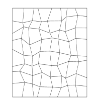
(a) mesh $\Omega^{1}_{h}$

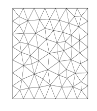
(b) mesh $\Omega^{2}_{h}$

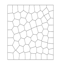
(c) mesh $\Omega^{3}_{h}$

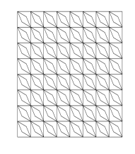
(d) mesh $\Omega^{4}_{h}$

Figure 1: Domain discretized with different meshes.

In order to test the convergence properties of the proposed VEM, we measure some errors as the difference between the exact solutions $(\psi,\theta)$ and adequate projections of the numerical solution $(\psi^{n}_{h},\theta^{n}_{h})$. More precisely, we consider the following quantities:

$${\tt E}(\psi,{\rm L}^{2},{\rm H}^{2}) :=\Big{(}\Delta t\sum_{n=1}^{N}|\psi(t_{n})-\Pi^{\mathbf{D},2}\psi^{n}_{h}|^{2}_{2,h}\Big{)}^{1/2},\qquad{\tt E}(\theta,{\rm L}^{2},{\rm H}^{1}):=\Big{(}\Delta t\sum_{n=1}^{N}|\theta(t_{n})-\Pi^{\nabla,1}\theta^{n}_{h}|^{2}_{1,h}\Big{)}^{1/2},$$ (6.1)

$${\tt E}(\psi,{\rm L}^{\infty},{\rm H}^{1}) :=|\psi(T)-\Pi^{\mathbf{D},2}\psi^{N}_{h}|_{1,h},\qquad\qquad\qquad\quad{\tt E}(\theta,{\rm L}^{\infty},{\rm L}^{2}):=\|\theta(T)-\Pi^{\nabla,1}\theta^{N}_{h}\|_{0,\Omega}.$$ (6.2)

Accordingly to Theorem 5.1, the expected convergence rate for the sum of the above norms is $\mathcal{O}(h+\Delta t)$.

6.1 Accuracy assessment

In our first example, we illustrate the accuracy in space and time of the proposed VEM (4.1), considering a manufactured exact solution on the square domain $\Omega:=(0,1)^{2}$, the time interval $[0,1]$ and force per unit mass ${\bf g}=(0,-1)^{T}$. We solve the Boussinesq system (2.1), taking the load terms ${\bf f}_{\psi}$ and $f_{\theta}$, boundary and initial conditions in such a way that the analytical solution is given by:

$$\boldsymbol{u}(x,y,t)=\begin{pmatrix}u_{1}(x,y,t)\\ u_{2}(x,y,t)\end{pmatrix}=\begin{pmatrix}\>\>(e^{10(t-1)}-e^{-10})\>x^{2}(1-x)^{2}(2y-6y^{2}+4y^{3})\\ -\>(e^{10(t-1)}-e^{-10})y^{2}(1-y)^{2}(2x-6x^{2}+4x^{3})\end{pmatrix},$$

$$p(x,y,t)=(e^{10(t-1)}-e^{-10})(\sin(x)\cos(y)+(\cos(1)-1)\sin(1)),$$

$$\psi(x,y,t)=(e^{10(t-1)}-e^{-10})x^{2}(1-x)^{2}y^{2}(1-y)^{2}\qquad\text{and}\qquad\theta(x,y,t)=u_{1}(x,y,t)+u_{2}(x,y,t).$$

In order to see the linear trend of the stream-function and temperature errors (6.1), predicted by Theorem 5.1, we refine simultaneously in space and time. More precisely, for each mesh family we consider the mesh refinements with $h=1/4,1/8,1/16,1/32$, and we use the same uniform refinements for the time variable. In particular, for the mesh $\Omega^{1}_{h}$, it can be seen along the diagonal of Table 1, the expected first order convergence for the stream-function and temperature errors (6.1).

In Figure 2, we display the errors (6.1) for the same simultaneous time and space refinements ($h=\Delta t=2^{-i}$, with $i=2,\ldots,5$), using the four mesh families. We notice that the rates of convergence predicted in Theorem 5.1 are attained by both unknowns.

${\tt E}(\psi,{\rm L}^{2};{\rm H}^{2})$
${\rm dofs}$		$1/4$	$1/8$	$1/16$	$1/32$	$1/64$
36	$1/4$	1.88912e-2	1.42183e-2	1.16131e-2	1.02912e-2	9.63665e-3
196	$1/8$	1.11333e-2	8.42107e-3	6.91546e-3	6.15400e-3	5.77765e-3
900	$1/16$	4.92223e-3	3.53363e-3	2.85747e-3	2.54826e-3	2.40427e-3
3844	$1/32$	3.61175e-3	2.11884e-3	1.46063e-3	1.21158e-3	1.11670e-3
15876	$1/64$	3.21002e-3	1.64565e-3	9.22443e-4	6.49802e-4	5.59824e-4
${\tt E}(\theta,{\rm L}^{2};{\rm H}^{1})$
36	$1/4$	1.74892e-2	1.34200e-2	1.11391e-2	9.96756e-3	9.38232e-3
196	$1/8$	1.02277e-2	7.88174e-3	6.66404e-3	6.05736e-3	5.75702e-3
900	$1/16$	5.32067e-3	3.65373e-3	2.93777e-3	2.64415e-3	2.51594e-3
3844	$1/32$	3.80377e-3	2.18463e-3	1.49484e-3	1.24874e-3	1.16084e-3
15876	$1/64$	3.37157e-3	1.71644e-3	9.52229e-4	6.64250e-4	5.69713e-4

Table 1: Accuracy assessment. Errors (6.1) using the VEM (4.1), with polynomial degrees $(k,\ell)=(2,1)$, physical parameters $\nu=\kappa=1$ and the mesh family mesh $\Omega^{1}_{h}$.

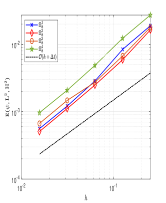
(a) Stream-function errors

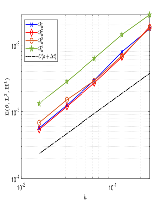
(b) Temperature errors

Figure 2: Accuracy assessment. Errors (6.1) for simultaneous space and time refinements, using the VEM (4.1) with polynomial degrees $(k,\ell)=(2,1)$, physical parameters $\nu=\kappa=1$ and the mesh families $\Omega^{i}_{h}$, $i=1,\ldots,4$.

In order to study the trend of the stream-function and temperature errors (6.2), we show in Table 2 the results considering again the mesh $\Omega^{1}_{h}$, with $h=\Delta t=2^{-i}$, with $i=2,\ldots,5$. In particular, we can observe that the rate of convergence in the mesh size $h$ seems higher than one; this is not fully surprising, since standard interpolation estimates (in space) for the norms in (6.2) indicate that, potentially, the discrete space could approximate the exact solution with order $\mathcal{O}(h^{2})$. In order to better investigate this aspect, in Figure 3 we display the errors (6.2) for space and time refinements given by $h=2^{-i}$ and $\Delta t=4^{-i}$, with $i=2,\ldots,5$, respectively, using the four mesh families. We notice that the rates of convergence seem indeed quadratic with respect to $h$.

${\tt E}(\psi,{\rm L}^{\infty};{\rm H}^{1})$
${\rm dofs}$		$1/4$	$1/8$	$1/16$	$1/32$	$1/64$
36	$1/4$	4.30301e-3	4.50090e-3	4.65255e-3	4.74590e-3	4.79749e-3
196	$1/8$	2.03865e-3	2.20110e-3	2.33234e-3	2.41662e-3	2.46443e-3
900	$1/16$	2.38767e-4	2.11074e-4	3.61809e-4	4.80109e-4	5.49619e-4
3844	$1/32$	7.26027e-4	4.35284e-4	2.05347e-4	6.71747e-5	4.99331e-5
15876	$1/64$	8.16241e-4	5.20174e-4	2.84604e-4	1.34953e-4	5.10645e-5
${\tt E}(\theta,{\rm L}^{\infty};{\rm L}^{2})$
36	$1/4$	3.44760e-3	3.94792e-3	4.28939e-3	4.48462e-3	4.58811e-3
196	$1/8$	9.85211e-4	1.44875e-3	1.82900e-3	2.06308e-3	2.19159e-3
900	$1/16$	5.96219e-4	2.98014e-4	3.26274e-4	4.64998e-4	5.57065e-4
3844	$1/32$	8.26668e-4	4.90632e-4	2.31786e-4	9.52686e-5	9.44396e-5
15876	$1/64$	8.90387e-4	5.68492e-4	3.13988e-4	1.53393e-4	6.48063e-5

Table 2: Accuracy assessment. Errors (6.2) using the VEM (4.1), with polynomial degrees $(k,\ell)=(2,1)$, the physical parameters $\nu=\kappa=1$ and the mesh family $\Omega^{1}_{h}$.

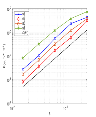
(a) Stream-function errors

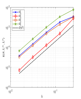
(b) Temperature errors

Figure 3: Accuracy assessment. Errors (6.2), using the VEM (4.1) with polynomial degrees $(k,\ell)=(2,1)$, the physical parameters $\nu=\kappa=1$ and the mesh families $\Omega^{i}_{h}$, $i=1,\ldots,4$.

6.2 Performance of the VEM for small viscosity

In this test we consider the square domain $\Omega:=(0,1)^{2}$, the time interval $[0,1]$ and force per unit mass ${\bf g}=(0,-1)^{T}$. We solve the Boussinesq system (2.1), taking the load terms ${\bf f}_{\psi}$ and $f_{\theta}$, boundary and initial conditions in such a way that the analytical solution is given by:

$$\boldsymbol{u}(x,y,t)=\begin{pmatrix}u_{1}(x,y,t)\\ u_{2}(x,y,t)\end{pmatrix}=\begin{pmatrix}-\cos(t)\sin(\pi x)\sin(\pi y)\\ -\cos(t)\cos(\pi x)\cos(\pi y)\end{pmatrix},$$

$$p(x,y,t)=\cos(t)(\sin(\pi x)+\cos(\pi y)-2/\pi),$$

$$\psi(x,y,t)=\frac{1}{\pi}\cos(t)\sin(\pi x)\cos(\pi y)\qquad\text{and}\qquad\theta(x,y,t)=u_{1}(x,y,t)+u_{2}(x,y,t).$$

The purpose of this experiment is to investigate the performance of the VEM (4.1) for small viscosity parameters. In Figure 4, we post the errors (6.1) of the stream-function variable obtained with the mesh sizes $h=1/4,1/8,1/16$ of $\Omega^{2}_{h}$, considering different values of $\nu$ and fixing the time step $\Delta t$ as $1/8$ and $1/16$ (see Figure 4(a) and Figure 4(b), respectively). It can observed that the solutions of our VEM are accurate even for small values of $\nu$. Larger stream-function errors appear for very small viscosity values.

We observe that this results are in accordance with the general observation that exactly divergence-free Galerkin methods are more robust with respect to small diffusion parameters, see for instance [50] (and also [15] in the VEM context). On the other hand, note that the scheme here proposed has no explicit stabilization of the convection term since this is not the focus of the present work (for instance, the natural norm associated to the stability of the discrete problem does not guarantee a robust control on the convection).

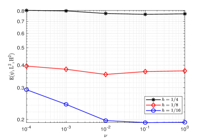
(a) Stream-function errors with $\Delta t=1/8$

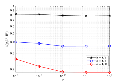
(b) Stream-function errors with $\Delta t=1/16$

Figure 4: Small viscosity test. Errors (6.1) of the VEM (4.1), for different values of $\nu$ and $\kappa=1$, using the meshes $\Omega^{2}_{h}$, polynomial degrees $(k,\ell)=(2,1)$.

6.3 Natural convection in a cavity with the left wall heating

In this last example we consider the $2$D natural convection benchmark problem, describing the behaviour of a incompressible flow in a squared cavity, which is heated at the left wall (see [59, 55, 44, 43, 57]). In particular, we consider the unitary square domain $\Omega=(0,1)^{2}$. The boundary conditions are given as follows: the temperature in the left and right walls are $\theta_{L}=1$ and $\theta_{R}=0$, respectively, while in the horizontal walls is $\partial_{{\bf n}}\theta=0$ (i.e., insulated, there is no heat transfer through these walls), no-slip boundary conditions are imposed for the fluid flow at all walls. In terms of the stream-function these conditions are given by: $\psi=\partial_{x}\psi=\partial_{y}\psi=0$ on $\Gamma$, as shown in Figure 5. The initial conditions are chosen as $\psi_{0}=-x+y$ and $\theta_{0}=1$ (so that the initial data does not satisfy the boundary conditions).

We consider the forces ${\bf f}_{\psi}=\boldsymbol{0}$, $f_{\theta}=0$ and ${\bf g}={\rm Pr}{\rm Ra}(0,1)^{T}$, where ${\rm Pr}$ and ${\rm Ra}$ denote the Prandtl and Rayleigh numbers, respectively. For the numerical experiment, we set the physical parameters as: $\nu={\rm Pr}=0.71$, ${\rm Ra}\in[10^{3},10^{6}]$ and $\kappa=1$.

(a) Boundary conditions

(b) mesh $\Omega^{5}_{h}$ with $h=1/8$

Figure 5: Natural convection cavity. Boundary conditions and domain discretized with mesh $\Omega^{5}_{h}$.

In order to compare our results with the existing bibliographic, we decompose the domain $\Omega$ using mesh $\Omega^{5}_{h}$ conformed by uniform squares (see Figure 5(b)). Moreover, the time step is $\Delta t=10^{-3}$ and final time $T=1$.

Streamlines and isotherms of the discrete solution obtained with our VEM (4.1) are posted in Figure 6, using ${\rm Ra}=10^{3},10^{4},10^{5},10^{6}$ and mesh size $h=1/64$. The results show well agreement with the results presented in the benchmark solutions in [59, 55, 44, 43, 57].

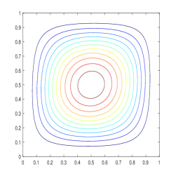
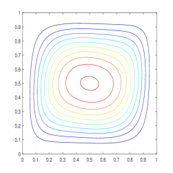
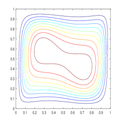
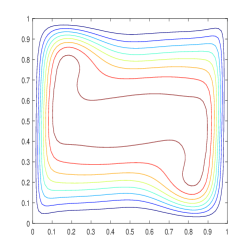
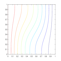
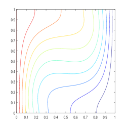
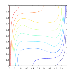
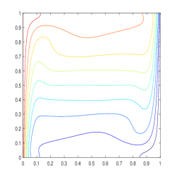
Figure 6: Natural convection cavity: streamlines (top panels) and isotherms (bottom panels), for ${\rm Ra}=10^{3},10^{4},10^{5}$ and $10^{6}$, respectively (from left to right).

Tables 3 and 4 present a quantitative comparison between our results and those obtained by the benchmark solutions in the above papers. Table 3 shows the maximum vertical velocity at $y=0.5$, for ${\rm Ra}=10^{4},10^{5}$ and $10^{6}$, while Table 4 shows the maximum horizontal velocity at $x=0.5$, using the same values of the Rayleigh number. Here the numbers in the parenthesis indicate the mesh size used by the respective reference. We can observe that the results show good agreement, even for higher Rayleigh numbers.

${\rm Ra}$	VEM	Ref [59]	Ref [55]	Ref [44]	Ref [43]	Ref [57]
$10^{4}$	19.56(64)	19.63(64)	19.51(41)	19.63(71)	19.90(71)	19.79(101)
$10^{5}$	68.46(64)	68.48(64)	68.22(81)	68.85(71)	70.00(71)	70.63(101)
$10^{6}$	216.37(64)	220.46(64)	216.75(81)	221.6(71)	228.0(71)	227.11(101)

Table 3: Natural convection cavity. Comparison of maximum vertical velocity $u_{1h}:=\Pi_{h}^{1}\partial_{y}\psi$ at $y=0.5$ with the VEM (4.1) and mesh $\Omega^{5}_{h}$ ($h=1/64$).

${\rm Ra}$	VEM	Ref [59]	Ref [55]	Ref [43]	Ref [57]
$10^{4}$	16.15(64)	16.19(64)	16.18(41)	16.10(71)	16.10(101)
$10^{5}$	34.80(64)	34.74(64)	34.81(81)	34.0(71)	34.00(101)
$10^{6}$	65.91(64)	64.81(64)	65.33(81)	65.40(71)	65.40(101)

Table 4: Natural convection cavity. Comparison of maximum horizontal velocity $u_{2h}:=-\Pi_{h}^{1}\partial_{x}\psi$ at $x=0.5$ with the VEM (4.1) and mesh $\Omega^{5}_{h}$ ($h=1/64$).

Finally, for the natural convection problem we investigate the heat transfer coefficient along the vertical walls of the cavity in terms of the local Nusselt number $({\rm Nu}_{local})$, which is defined by: ${\rm Nu}_{local}(x,y):=-\partial_{{\bf n}}\theta(x,y)$. Figure 7 describes the variation of local Nusselt number at hot wall and cold wall, for different values of the Rayleigh number. It can be seen that the results show good agreement with the results presented in [59, 55, 44, 43, 57].

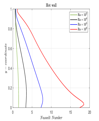
(a) Nusselt in the hot wall

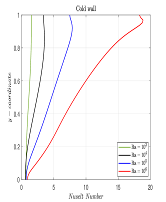
(b) Nusselt in the cold wall

Figure 7: Natural convection cavity. Nusselt number along the hot wall (left) and the cold wall (right) for varying Rayleigh numbers, using the VEM (4.1) and mesh $\Omega^{5}_{h}$, with $h=1/64$.

References

- [1] D. Adak, D. Mora, S. Natarajan and A. Silgado, A virtual element discretization for the time dependent Navier-Stokes equations in stream-function formulation, ESAIM Math. Model. Numer. Anal., 55(5), (2021), pp. 2535–2566.
- [2] R.A. Adams and J.J.F. Fournier, Sobolev Spaces, 2nd ed., Academic Press, Amsterdam, 2003.
- [3] B. Ahmad, A. Alsaedi, F. Brezzi, L.D. Marini and A. Russo, Equivalent projectors for virtual element methods, Comput. Math. Appl., 66, (2013), pp. 376–391.
- [4] R. Aldbaissy, F. Hecht, G. Mansour and T. Sayah, A full discretisation of the time-dependent Boussinesq (buoyancy) model with nonlinear viscosity, Calcolo, 55(4), (2018), Paper No. 44, 49.
- [5] R. Agroum, C. Bernardi and J. Satouri, Spectral discretization of the time-dependent Navier-Stokes problem coupled with the heat equation, Appl. Math. Comput., 268, (2015), pp. 59–82.
- [6] P.F. Antonietti, L. Beirão da Veiga, D. Mora and M. Verani, A stream virtual element formulation of the Stokes problem on polygonal meshes, SIAM J. Numer. Anal., 52, (2014), pp. 386–404.
- [7] P.F. Antonietti, L. Beirão da Veiga, S. Scacchi and M. Verani, A virtual element method for the Cahn–Hilliard equation with polygonal meshes, SIAM J. Numer. Anal., 54, (2016), pp. 36–56.
- [8] P.F. Antonietti, G. Manzini, S. Scacchi and M. Verani, A review on arbitrarily regular conforming virtual element methods for second- and higher-order elliptic partial differential equations. Math. Models Methods Appl. Sci. 31(14), (2021), pp. 2825–2853.
- [9] P.F. Antonietti, G. Vacca and M. Verani, Virtual element method for the Navier–Stokes equation coupled with the heat equation, arXiv:2205.00954v1 [math.NA], (2022).
- [10] L. Beirão da Veiga, F. Brezzi, A. Cangiani, G. Manzini, L.D. Marini and A. Russo, Basic principles of virtual element methods, Math. Models Methods Appl. Sci., 23, (2013), pp. 199–214.
- [11] L. Beirão da Veiga, F. Brezzi, L.D. Marini and A. Russo, Virtual element method for general second-order elliptic problems on polygonal meshes, Math. Models Methods Appl. Sci., 26(4), (2016), pp. 729–750.
- [12] L. Beirão da Veiga, F. Dassi and G. Vacca, The Stokes complex for virtual elements in three dimensions, Math. Models Methods Appl. Sci., 30(3), (2020), pp. 477–512.
- [13] L. Beirão da Veiga, C. Lovadina and A. Russo, Stability analysis for the virtual element method, Math. Models Methods Appl. Sci., 27(13), (2017), pp. 2557–2594.
- [14] L. Beirão da Veiga, C. Lovadina and G. Vacca, Divergence free virtual elements for the Stokes problem on polygonal meshes, ESAIM Math. Model. Numer. Anal., 51, (2017), pp. 509–535.
- [15] L. Beirão da Veiga, C. Lovadina and G. Vacca, Virtual elements for the Navier-Stokes problem on polygonal meshes, SIAM J. Numer. Anal., 56(3), (2018), pp. 1210–1242.
- [16] L. Beirão da Veiga and G. Manzini, A virtual element method with arbitrary regularity, IMA J. Numer. Anal., 34, (2014), pp. 759–781.
- [17] L. Beirão da Veiga and G. Manzini, Residual a posteriori error estimation for the virtual element methods for elliptic problems, ESAIM Math. Model. Numer. Anal., 49(2), (2015), pp. 577–599.
- [18] L. Beirão da Veiga, D. Mora and G. Rivera, Virtual elements for a shear-deflection formulation of Reissner-Mindlin plates, Math. Comp., 88, (2019), pp. 149–178.
- [19] L. Beirão da Veiga, D. Mora and G. Vacca, The Stokes complex for virtual elements with application to Navier-Stokes flows, J. Sci. Comput., 81(2), (2019), pp. 990–1018.
- [20] L. Beirão da Veiga, A. Pichler and G. Vacca, A virtual element method for the miscible displacement of incompressible fluids in porous media, Comput. Methods Appl. Mech. Engrg., 375, (2021), Paper No. 113649, 35 pp.
- [21] P.L. Betts and V. Haroutunian, A stream function finite element solution for two-dimensional natural convection with accurate representation of Nusselt number variations near a corner, Int. J. Numer. Methods Fluids., 3, (1983), pp. 605–622.
- [22] C. Bernardi, B. Métivet and B. Pernaud-Thomas, Couplage des équations de Navier-Stokes et de la chaleur: le modèle et son approximation par éléments finis. ESAIM Math. Model. Numer. Anal., 29(7), (1995), pp. 871–921.
- [23] J. Boland and W. Layton, An analysis of the finite element method for natural convection problems, Numer. Methods Partial Differential Equations, 2, (1990), pp. 115–126.
- [24] S.C. Brenner and R.L. Scott, The Mathematical Theory of Finite Element Methods, Springer, New York, 2008.
- [25] S.C. Brenner and L.Y. Sung, Virtual element methods on meshes with small edges or faces, Math. Models Methods Appl. Sci., 28(7), (2018), pp. 1291–1336.
- [26] F. Brezzi and L.D. Marini, Virtual elements for plate bending problems, Comput. Methods Appl. Mech. Engrg., 253, (2013), pp. 455–462.
- [27] E. Cáceres, G.N. Gatica and F. Sequeira, A mixed virtual element method for the Brinkman problem, Math. Models Methods Appl. Sci., 27, (2017), pp. 707–743.
- [28] A. Cangiani, G. Manzini and O.J. Sutton, Conforming and nonconforming virtual element methods for elliptic problems, IMA J. Numer. Anal., 37, (2017), pp. 1317–1354.
- [29] L. Chen and J Huang, Some error analysis on virtual element methods, Calcolo, 55(1), (2018), pp. 5–23.
- [30] A. Chernov, C. Marcati and L. Mascotto, - and - virtual elements for the Stokes problem, Adv. Comput. Math., 47, (2021), article number: 24, pp. 1–31.
- [31] C. Chinosi and L.D. Marini, Virtual element method for fourth order problems: -estimates, Comput. Math. Appl., 72(8), (2016), pp. 1959–1967.
- [32] E. Colmenares, G. N. Gatica and R. Oyarzúa, Analysis of an augmented mixed-primal formulation for the stationary Boussinesq problem, Numer. Methods Partial Differential Equations, 32(2), (2016), pp 445–478.
- [33] H. Dallmann and D. Arndt, Stabilized finite element methods for the Oberbeck-Boussinesq model, J. Sci. Comput., 69(1), (2016), pp. 244–273.
- [34] M. Dehghan, Z. Gharibi and R. Ruiz-Baier, Optimal error estimates of coupled and divergence-free virtual element methods for the Poisson–Nernst–Planck/Navier–Stokes equations, arXiv:2207.02455 [math.NA], (2022).
- [35] J. de Frutos, B. García-Archilla and Julia Novo, Grad-div stabilization for the time-dependent Boussinesq equations with inf-sup stable finite elements, Appl. Math. Comput., 349, (2019), pp. 281–291.
- [36] D. Frerichs and C. Merdon, Divergence-preserving reconstructions on polygons and a really pressure-robust virtual element method for the Stokes problem, IMA J. Numer. Anal., 42(1), (2022), pp. 597–619.
- [37] G.N. Gatica, M. Munar and F. Sequeira, A mixed virtual element method for the Boussinesq problem on polygonal meshes, J. Comput. Math., 39(3), (2021), pp. 392–427.
- [38] V. Girault and P.A. Raviart, Finite Element Methods for Navier-Stokes Equations, Springer-Verlag, Berlin, 1986.
- [39] Q. Guan, Some estimates of virtual element methods for fourth order problems, Electronic Research Archive, 29(6), (2021), pp. 4099–4118.
- [40] J. Heywood and R. Rannacher, Finite element approximation of the nonstationary Navier- Stokes problem, IV. Error analysis for second-order time discretization, SIAM J. Numer. Anal., 19, (1990), pp. 275–311.
- [41] S. A. Lorca and J.L Boldrini, The initial value problem for a generalized Boussinesq model. Nonlinear Anal., 36(4), (1999) Ser. A: Theory Methods, pp. 457–480.
- [42] J.G. Liu, C. Wang and H. Johnston, A fourth order scheme for incompressible Boussinesq equations, J. Sci. Comput., 18(2), (2003), pp. 253–285.
- [43] M.T. Manzari, An explicit finite element algorithm for convective heat transfer problems, Internat. J. Numer. Methods Heat Fluid Flow, 9, (1999), pp. 860–877.
- [44] N. Massarotti, P. Nithiarasu and O.C. Zienkiewicz, Characteristic-Based-Split (CBS) algorithm for incompressible flow problems with heat transfer, Internat. J. Numer. Methods Heat Fluid Flow, 8, (1998), pp. 969–990.
- [45] D. Mora, G. Rivera and R. Rodríguez, A virtual element method for the Steklov eigenvalue problem, Math. Models Methods Appl. Sci., 25, (2015), pp. 1421–1445.
- [46] D. Mora, C. Reales and A. Silgado, A -virtual element method of high order for the Brinkman equations in stream function formulation with pressure recovery, IMA J. Numer. Anal., Article in press, DOI: https://doi.org/10.1093/imanum/drab078.
- [47] D. Mora and A. Silgado, A virtual element method for the stationary quasi-geostrophic equations of the ocean, Comput. Math. Appl., 116, (2022), pp. 212–228.
- [48] H. Morimoto, Nonstationary Boussinesq equations, J. Fac. Sci. Univ. Tokyo Sect. IA Math., 39(1), (1992), pp. 61–75.
- [49] R. Oyarzúa, T. Qin and D. Schötzau, An exactly divergence-free finite element method for a generalized Boussinesq problem, IMA J. Numer. Anal., 34(3), (2014), pp. 1104–1135.
- [50] P. W. Schroeder and G. Lube Pressure-robust analysis of divergence-free and conforming FEM for evolutionary incompressible Navier–Stokes flows, J. Numer. Math., 25(4), (2017), pp. 249–276.
- [51] W.N.R. Stevens, Finite element, stream function–vorticity solution of steady laminar natural convection, Int. J. Numer. Methods Fluids, 2, (1982), pp. 349–366.
- [52] M. Tabata and D. Tagami, Error estimates of finite element methods for nonstationary thermal convection problems with temperature-dependent coefficients, Numer. Math., 100(2), (2005), pp. 351–372.
- [53] Z. Tian and Y. Ge, A fourth-order compact finite difference scheme for the steady stream function-vorticity formulation of the Navier-Stokes/Boussinesq equations, Internat. J. Numer. Methods Fluids, 41(5), (2003), pp. 495–518.
- [54] G. Vacca and L. Beirão da Veiga, Virtual element methods for parabolic problems on polygonal meshes, Numer. Methods Partial Differential Equations, 31(6), (2015), pp. 2110–2134.
- [55] D. de Vahl Davis, Natural convection of air in a square cavity: A benchmark solution, Internat. J. Numer. Methods Fluids, 3, (1983), pp. 249–264.
- [56] N. Verma and S. Kumar, Lowest order virtual element approximations for transient Stokes problem on polygonal meshes, Calcolo, 58(4), (2021), Paper No. 48, 35 pp.
- [57] D.C. Wan, B.S.V. Patnaik and G.W. Wei, A new benchmark quality solution for the buoyancy-driven cavity by discrete singular convolution, Numer. Heat Transfer, 40, (2001), pp. 199–228.
- [58] C. Wang, J.G. Liu and H. Johnston, Analysis of a fourth order finite difference method for the incompressible Boussinesq equations, Numer. Math., 97(3), (2004), pp. 555–594.
- [59] Y. Zhang, Y. Hou and J. Zhao, Error analysis of a fully discrete finite element variational multiscale method for the natural convection problem, Comput. Math. Appl., 68(4), (2014), pp. 543–567.