The good-bad-ugly system near spatial infinity on flat spacetime

Abstract

A model system of equations that serves as a model for the Einstein field equation in generalised harmonic gauge called the good-bad-ugly system is studied in the region close to null and spatial infinity in Minkowski spacetime. This analysis is performed using H. Friedrich’s cylinder construction at spatial infinity and defining suitable conformally rescaled fields. The results are translated to the physical set up to investigate the relation between the polyhomogeneous expansions arising from the analysis of linear fields using the $i^{0}$-cylinder framework and those obtained through a heuristic method based on Hörmander’s asymptotic system.

Keywords: cylinder at spatial infinity, null infinity, asymptotic system.

1 Introduction

One of the most emblematic results in the classical theory of asymptotics in general relativity is the peeling theorem [1, 2, 3]. The general term of “peeling” refers to the decay of the Weyl tensor in the asymptotic region of the spacetime. The classical peeling theorem [3] shows that, if a spacetime admits a smooth conformal extension then the components of the Weyl tensor decay as integer powers of a suitable parameter along the generators of outgoing light cones. The genericity of this crucial smoothness assumption has been put in question from the perspective of the initial value problem. There exist a considerable number of results —[4, 5, 6, 7, 8, 9, 10, 11]— showing, with varying levels of rigour and different standpoints, that generically, the gravitational field would satisfy at best a restricted peeling behaviour. Comparing these different results becomes a non-trivial task due to the diverse approaches taken in each case and the variety of gauges used to derive the results.

Recently, in [4] it was shown, exploiting a heuristic method introduced in [12], that in generalised harmonic gauge, the components of the Weyl tensor admit a polyhomogeneous expansion. The heuristic method put forward in [12], is based on a generalisation of Hörmander’s asymptotic system —see [13, 14, 15]. The general method used in [12] finds applicability and is tailored for a formulation of the Einstein field equations in generalised harmonic gauge which is designed for numerical investigations via suitably hyperboloidal initial value problems exploiting the dual frame formalism [16, 17].

Interestingly, there exist other body of work —see [11, 18, 19, 9, 20]— based on a distinctively different approach, the conformal Einstein field equations, giving seemingly similar polyhomogeneous expansions for the Weyl tensor. The polyhomogeneous expansions in [11, 19, 9] are obtained through the analysis of the components of the rescaled Weyl spinor close to spatial and null infinity. To do so, the framework of the cylinder at spatial infinity is employed. The cylinder at spatial infinity is a formalism developed to study the behaviour of the gravitational field in the region where null and spatial infinity meet —the critical sets— by means of the extended conformal Einstein field equations written in a gauge adapted to a special class of curves known as conformal geodesics [11, 21]. This special gauge around which the $i^{0}$-cylinder formalism is constructed is known as the $F$-gauge. Unfortunately, the relation between the $F$-gauge and other more traditional gauges is not simple to establish in general. However, there is a particular case where this gauge and the construction of the cylinder at spatial infinity can be obtained in an explicit closed form: the Minkowski spacetime. This special conformal representation of the Minkowski spacetime has been used as a model to understand the behaviour of fields propagating in the vicinity of spatial infinity of asymptotically flat spacetimes and the consequences of the degeneracy of the equations in the critical sets —see [22, 23, 24, 25, 26, 27, 28]. Crucially, one of these consequences is that even linear fields propagating in this conformal representation of the Minkowski spacetime ($i^{0}$-cylinder background) will develop logarithmic terms at the critical sets which spread out to null infinity —see [22, 23, 25, 29]. Although it has been shown that the non-linearities in the conformal Einstein field equations will generate further logarithmic terms —see [30], the analysis of linear fields about the given background already serves as a basis to develop intuition into what is the minimal regularity of the field that can be be expected close to the critical sets.

On the other hand, the basic model under which the general method of [12] was constructed is the good-bad-ugly (GBU) system of equations. This system is constituted by three fields which satisfy wave equations with non-linearities that mimic the worst of those present in the Einstein field equations in generalised harmonic gauge. In this paper, the GBU model equation on flat spacetime is solved using the methods of the cylinder at spatial infinity. The solution is obtained by conformally transforming the equations and fields to the $i^{0}$-cylinder background, defining a corresponding “unphysical” GBU system, then solving for the unphysical good, bad and ugly fields close to spatial infinity and then translating back the solution to the physical picture and comparing the results with those obtained in [12]. In doing so, we clarify the relation between the logarithmic terms obtained through the two methods and establish a base analysis for future investigations in the non-linear case.

Notations and Conventions

Most of the literature of Friedrich’s cylinder at spatial infinity uses the signature convention natural to spinors $(+,-,-,-)$. Nonetheless, since spinor formalism will not be used in this article, the signature convention for a Lorentzian spacetime metric will be the more standard $(-,+,+,+)$. Fields defined on the physical setup can be identified by the $\;\tilde{}\;$ symbol, while the unphysical (compactified) ones will not have such decoration. Latin and Greek indices will be used as abstract and coordinate indices respectively.

2 The cylinder at spatial infinity

The term cylinder at spatial infinity is broadly used to refer to a general framework to study conformal extensions of asymptotically flat spacetimes in a neighbourhood of spatial infinity using the conformal Einstein field equations —see [11, 21]. While these conformal extensions are known in general only in an abstract (non-explicit) way, for the Minkowski spacetime one can write closed and explicit expressions. Although most of the expressions given in this section have been reported already —see for instance [11, 31, 22, 24, 25, 29]— in the discussion presented here the emphasis is placed on making contact with the physical structures and the translation of some of the $i^{0}$-cylinder results to the physical set-up.

2.1 The $i^{0}$-cylinder conformal extension of the Minkowski spacetime

Let $\tilde{{\bm{\eta}}}$ be a Minkowski metric and let $\tilde{x}^{\mu}=(\tilde{t},\tilde{x}^{i})$, denote physical Cartesian coordinates. In these coordinates the Minkowski metric reads:

$$\tilde{{\bm{\eta}}}=\eta_{\mu\nu}\mathbf{d}\tilde{x}^{\mu}\otimes\mathbf{d}\tilde{x}^{\nu},$$ (1)

where $\eta_{\mu\nu}=\text{diag}(-1,1,1,1)$. Introducing physical polar coordinates defined by $\tilde{\rho}^{2}=\delta_{ij}\tilde{x}^{i}\tilde{x}^{j}$ where $\delta_{ij}=\text{diag(1,1,1)}$ and an arbitrary choice of coordinates on $\mathbb{S}^{2}$ one has

$$\tilde{{\bm{\eta}}}=-\mathbf{d}\tilde{t}\otimes\mathbf{d}\tilde{t}+\mathbf{d}\tilde{\rho}\otimes\mathbf{d}\tilde{\rho}+\tilde{\rho}^{2}\mathbf{\bm{\sigma}},$$ (2)

with $\tilde{t}\in(-\infty,\infty)$, $\tilde{\rho}\in[0,\infty)$ where $\bm{\sigma}$ denotes the standard metric on $\mathbb{S}^{2}$. The procedure to obtain the cylinder representation of spatial infinity is as follows: First, introduce inversion Cartesian coordinates $x^{\mu}=(t,x^{i})$

$$x^{\mu}={\tilde{x}^{\mu}}/{\tilde{X}^{2}},\qquad\tilde{X}^{2}\equiv\tilde{\eta}_{\mu\nu}\tilde{x}^{\mu}\tilde{x}^{\nu}.$$ (3)

A direct calculation shows that the inverse transformation is

$$\tilde{x}^{\mu}=x^{\mu}/X^{2},\qquad X^{2}=\eta_{\mu\nu}x^{\mu}x^{\nu}.$$ (4)

which is valid in the region where $\tilde{X}^{2}>0$, namely, in the complement of the lightcone at the origin in the Minkowski spacetime.

Remark 1.

There is a sign difference in equation (3) respect to other discussions in the literature —see [24, 25, 29]— which is due to the use of a different signature convention.

Using these coordinates, the following conformal (inversion) extension of the Minkowski spacetime is identified

$${\bm{g}}_{I}=\Xi^{2}\hskip 1.42262pt\tilde{{\bm{\eta}}},$$ (5)

where ${\bm{g}}_{I}=\eta_{\mu\nu}\mathbf{d}x^{\mu}\otimes\mathbf{d}x^{\nu}$ and $\Xi=X^{2}$. Observe that $X^{2}=1/\tilde{X}^{2}$. Now, define an unphysical polar radial coordinate via $\rho^{2}=\delta_{ij}x^{i}x^{j}$. In the unphysical polar coordinates, the rescaled metric ${\bm{g}}_{I}$ and conformal factor $\Xi$ read

$${\bm{g}}_{I}=-\mathbf{d}t\otimes\mathbf{d}t+\mathbf{d}\rho\otimes\mathbf{d}\rho+\rho^{2}\mathbf{\bm{\sigma}},\qquad\Xi=\rho^{2}-t^{2},$$ (6)

with $t\in(-\infty,\infty)$ and $\rho\in\leavevmode\nobreak\ [0,\infty)$. Although ${\bm{g}}_{I}$ is again the Minkowski metric notice that the roles of the origin $\mathcal{O}$ and spatial infinity $i^{0}$ are swapped. In other words, in this representation, $i^{0}$ corresponds to the point with coordinates $(t=0,\rho=0)$ in $(\mathbb{R}^{4},{\bm{g}}_{I})$. To prepare for the upcoming discussion, it will be useful to write the coordinate transformations (3) and (4) in terms of the physical and unphysical (inversion) polar coordinates:

$$\tilde{t}=\frac{t}{\rho^{2}-t^{2}},\qquad\tilde{\rho}=\frac{\rho}{\rho^{2}-t^{2}}.$$ (7)

The inverse transformation is given by

$$t=\frac{\tilde{t}}{\tilde{\rho}^{2}-\tilde{t}^{2}},\qquad\rho=\frac{\tilde{\rho}}{\tilde{\rho}^{2}-\tilde{t}^{2}}.$$ (8)

where we have chosen the positive root in the expression defining the respective radial coordinates. To arrive to the relevant conformal representation of the Minkowski spacetime the following change of coordinates is introduced

$$t=\rho\tau.$$ (9)

The unphysical coordinate system $(\tau,\rho)$ will be called $F$-coordinates. In these coordinates the metric ${\bm{g}}_{I}$ is written as

$${\bm{g}}_{I}=-\rho^{2}\mathbf{d}\tau\otimes\mathbf{d}\tau+(1-\tau^{2})\mathbf{d}\rho\otimes\mathbf{d}\rho-\rho\tau\mathbf{d}\rho\otimes\mathbf{d}\tau-\rho\tau\mathbf{d}\tau\otimes\mathbf{d}\rho+\rho^{2}{\bm{\sigma}}.$$

Finally, by rescaling the ${\bm{g}}_{I}$ as

$${\bm{g}}\equiv\frac{1}{\rho^{2}}{\bm{g}}_{I},$$ (10)

one obtains the conformal representation of the Minkowski spacetime adapted to the cylinder at spatial infinity. Composing the coordinate transformations and the conformal transformations one concludes that the relation between the (physical) Minkowski metric $\tilde{\bm{\eta}}$ and the (unphysical) $i^{0}$-cylinder metric ${\bm{g}}$ is given by

$${\bm{g}}=\Theta^{2}\tilde{\bm{\eta}}$$ (11)

where

$${\bm{g}}=-\mathbf{d}\tau\otimes\mathbf{d}\tau+\frac{(1-\tau^{2})}{\rho^{2}}\mathbf{d}\rho\otimes\mathbf{d}\rho-\frac{\tau}{\rho}\mathbf{d}\rho\otimes\mathbf{d}\tau-\frac{\tau}{\rho}\mathbf{d}\tau\otimes\mathbf{d}\rho+{\bm{\sigma}}.$$

and

$$\Theta:=\frac{\Xi}{\rho}$$ (12)

consistent with the bookkeeping naming conventions of Section Notations and Conventions, the metric ${\bm{g}}$ will be regarded as the metric of the unphysical spacetime while $\tilde{\bm{\eta}}$ as the metric of the physical spacetime. These naming conventions stem from the fact that the unphysical metric ${\bm{g}}$ corresponds to an explicit solution to the conformal Einstein field equations written in a gauge adapted to conformal geodesics —see [11, 21, 31, 22, 24, 25, 29] for further discussion and definitions. To simplify the terminology when discussing fields propagating in this geometry we will refer to it simply as the $i^{0}$-cylinder background. To better describe the geometry of the cylinder at spatial infinity it is convenient to introduce, the following ${\bm{g}}$-null frame —which in the following will be referred to as the $F$-frame:

$$\bm{\ell}=(1+\tau)\bm{\partial}_{\tau}{}-\rho\bm{\partial}_{\rho}{},\qquad\bm{\underline{\ell}}=(1-\tau)\bm{\partial}_{\tau}{}+\rho\bm{\partial}_{\rho}{},\qquad\bm{\partial}_{+}{},\qquad\qquad\bm{\partial}_{-}{}.$$ (13)

The corresponding dual coframe is given by

$$\bm{\ell}^{\flat}=-\mathbf{d}\tau-\frac{1}{\rho}\big{(}1+\tau\big{)}\mathbf{d}\rho,\qquad\bm{\underline{\ell}}^{\flat}=-\mathbf{d}\tau{}+\frac{1}{\rho}\big{(}1-\tau\big{)}\mathbf{d}\rho,\qquad\bm{\omega}^{+},\qquad\bm{\omega}^{-}.$$

In these expressions $\bm{\partial}_{\pm}$ and $\bm{\omega}^{\pm}$ represent an arbitrary null frame and coframe on $\mathcal{Q}\approx\mathbb{S}^{2}$, denoting the surfaces of constant $\tau$ and constant $\rho$ so that

$$\bm{\sigma}=2(\bm{\omega}^{+}\otimes\bm{\omega}^{-}+\bm{\omega}^{-}\otimes\bm{\omega}^{+}),\qquad\bm{\sigma}^{\flat}=\frac{1}{2}(\bm{\partial}_{+}\otimes\bm{\partial}_{-}+\bm{\partial}_{-}\otimes\bm{\partial}_{+}).$$ (14)

This frame is Lie dragged along the $\bm{\partial}_{\tau}$ and $\bm{\partial}_{\rho}$ directions, imposing that $[\bm{\partial}_{\tau},\bm{\partial}_{\pm}]=[\bm{\partial}_{\rho},\bm{\partial}_{\pm}]=0$ —see discussion in Appendix of [24]. In accordance with the conventions of this article, the metric then reads

$$g_{ab}=\ell_{(a}\underline{\ell}_{b)}-\omega^{+}_{(a}\omega^{-}_{b)}\,,$$ (15)

so that the normalisation of the tetrad is $\ell_{a}\underline{\ell}^{a}=-\omega^{+}_{a}\partial_{-}^{a}=-2$ while all the other contractions vanish. The relevance of the geometry of the cylinder at spatial infinity for Minkowski spacetime, is that, in this representation future and past null infinity are located at

$$\mathscr{I}^{+}\equiv\{p\in\mathcal{M}\;\rvert\;\tau(p)=1\},\qquad\mathscr{I}^{-}\equiv\{p\in\mathcal{M}\;\rvert\;\tau(p)=-1\},$$ (16)

and the following sets can be distinguished:

$$I\equiv\{p\in\mathcal{M}\;\rvert\;\;|\tau(p)|<1,\;\rho(p)=0\},\qquad I^{0}\equiv\{p\in\mathcal{M}\;\rvert\;\tau(p)=0,\;\rho(p)=0\},$$

$$I^{+}\equiv\{p\in\mathcal{M}\;\rvert\;\tau(p)=1,\;\rho(p)=0\},\qquad I^{-}\equiv\{p\in\mathcal{M}\;\rvert\;\tau(p)=-1,\;\rho(p)=0\}.$$

From the last expressions it can be noticed that spatial infinity $i^{0}$ has been blown up to the cylinder $I$. Moreover, different cuts of $I$ can be identified: $I^{0}$ denotes the intersection of the time symmetric hypersurface $\tau=0$ and $I$ and the critical sets $I^{\pm}$ represent the region where spatial and future/past null infinity meet, where evolution PDEs typically degenerate —see [11, 22, 24, 25, 29].

2.2 Relation to the physical coordinates and physical frame

The relation between the $F$-coordinates and the physical polar coordinates is:

$$\tau=\frac{\tilde{t}}{\tilde{\rho}},\qquad\rho=\frac{\tilde{\rho}}{\tilde{\rho}^{2}-\tilde{t}^{2}},$$ (17)

and the inverse transformation is

$$\tilde{t}=\frac{\tau}{\rho(1-\tau^{2})},\qquad\tilde{\rho}=\frac{1}{\rho(1-\tau^{2})}.$$ (18)

Unwrapping the definitions, the conformal factor $\Theta$ in $F$-coordinates and physical coordinate respectively, reads

$$\Theta=\rho(1-\tau^{2})=\frac{1}{\tilde{\rho}}$$ (19)

Hence, the relations in (18) can be succinctly rewritten as

$$\tilde{t}=\frac{\tau}{\Theta},\qquad\tilde{\rho}=\frac{1}{\Theta}.$$ (20)

For the upcoming calculations it will be convenient to introduce the physical advanced and retarded times

$$\tilde{u}=\tilde{t}-\tilde{\rho},\qquad\tilde{v}=\tilde{t}+\tilde{\rho}$$ (21)

The associated physical null vectors

$$L^{a}=-\tilde{\eta}^{ab}\tilde{\nabla}_{b}\tilde{u},\qquad\underline{L}^{a}=-\tilde{\eta}^{ab}\tilde{\nabla}_{b}\tilde{v},$$ (22)

explicitly read

$$L=\bm{\partial}_{\tilde{t}}+\bm{\partial}_{\tilde{\rho}},\qquad\underline{L}=\bm{\partial}_{\tilde{t}}-\bm{\partial}_{\tilde{\rho}}.$$ (23)

These vectors can be complemented with a pair of complex null vectors so that the physical null frame $\{L,\;\underline{L},\;\tilde{\bm{\omega}}^{+},\tilde{\bm{\omega}}^{-}\}$ reads

$$L=\bm{\partial}_{\tilde{t}}+\bm{\partial}_{\tilde{\rho}},\qquad\underline{L}=\bm{\partial}_{\tilde{t}}-\bm{\partial}_{\tilde{\rho}},\qquad\tilde{\omega}^{+}=\tilde{\rho}^{-1}\bm{\partial}_{+},\qquad\tilde{\omega}^{-}=\tilde{\rho}^{-1}\bm{\partial}_{-},$$ (24)

with the normalisation understood to be taken with respect to the physical Minkowski metric $\tilde{{\bm{\eta}}}$

$$\tilde{\eta}_{ab}L^{a}\underline{L}^{b}=-\tilde{\eta}_{ab}\tilde{\omega}^{a}_{+}\tilde{\omega}^{a}_{-}=-2.$$ (25)

This normalisation implies that the physical metric can be written as

$$\tilde{\eta}_{ab}=L_{(a}\underline{L}_{b)}-\tilde{\omega}^{+}_{(a}\tilde{\omega}^{-}_{b)}.$$ (26)

Remark 2.

Consistent with the previously stated conventions to distinguish the physical vs the unphysical fields, the physical null vectors should be denoted by the symbols $\tilde{\bm{\ell}}$ and $\tilde{\underline{\bm{\ell}}}$. Nonetheless, to simplify the notation and to align it with conventions of [9, 12, 13], the physical outgoing and incoming null vectors have been denoted with $L$ and $\underline{L}$ instead. Observe that with the current conventions an orthonormal frame can be constructed so that the timelike legs of such tetrads would read $\tilde{{\bm{e}}}_{0}=\frac{1}{2}(L+\underline{L})=\bm{\partial}_{\tilde{t}}$ and ${{\bm{e}}}_{0}=\frac{1}{2}({\bm{\ell}}+{\bm{\underline{\ell}}})=\bm{\partial}_{\tau}$.

For the calculations to follow, it will be necessary to spell out not only the relation between the coordinates but also the relation between the $F$-frame and the physical frames. A straightforward calculation using equations (13), (22), (17) and (18) gives the following

Proposition 1.

The relation between the $F$-frame and the physical frame —as given in equations (13) and (22), in the $i^{0}$-cylinder conformal extension of the Minkowski spacetime is given by

$$L=\Theta\kappa^{-1}\bm{\ell},\qquad\underline{L}=\Theta\kappa\bm{\underline{\ell}},\qquad\tilde{\bm{\partial}}_{\pm}^{a}=\Theta\bm{\partial}_{\pm}^{a},$$ (27)

where the conformal factor in $F$-coordinates and physical coordinates reads

$$\Theta:=\rho(1-\tau^{2})=\frac{1}{\tilde{\rho}}$$ (28)

and, similarly, the boost parameter $\kappa$ is given by

$$\kappa:=\frac{1+\tau}{1-\tau}=-\frac{\tilde{v}}{\tilde{u}}.$$ (29)

Remark 3.

The last result simply emphasises that the relation between the physical and unphysical frame is not only a conformal transformation but also a boost encoded in $\kappa$. Observe that $\kappa$ and $\kappa^{-1}$ diverge at $\mathscr{I}^{-}$ and $\mathscr{I}^{+}$ respectively; in particular, they diverge at the critical sets $I^{\pm}$ but are well defined elsewhere in the cylinder $I$. A crucial observation for the subsequent discussion is that the boost factor $\kappa$ —as given in equation (29)— can be written as the quotient between the physical advanced and retarded times.

Although the previous calculation is very simple, identifying the Lorentz transformation between the frames is crucial for practical applications of the $i^{0}$-cylinder framework. An example of this is that clarifying the relation between the $F$-frame and the NP-frame is central to compute conserved quantities at $\mathscr{I}$ —see for instance [32, 31, 24].

3 The GBU model close to spatial infinity

In [12], through an approach based on Hörmander’s asymptotic system, formal polyhomogeneous expansions near null infinity were obtained for a class of model equations called good-bad-ugly. The motivation for these model equations is that they mimic the non-linearities found in the Einstein field equations in harmonic gauge. Moreover, in [4] these expansions were used to obtain formal asymptotic expressions for the Weyl scalars. These were then used to assess the peeling properties of the gravitational field arising from an initial value problem using the Einstein field equations in generalised harmonic gauge. On the other hand, in [11, 31, 20, 9, 33] similar looking expansions have been obtained for the rescaled Weyl spinor using the conformal Einstein field equations. In this section we analyse the model equations of [12] from the point of view of conformal methods. Specifically, exploiting the framework of Friedrich’s cylinder at spatial infinity to understand if the logarithmic terms in [9, 33] and [12] —sourcing the violation of peeling in [4]— are related or not. To do so, we perform this calculation not on the full non-linear case of the Einstein field equations but on a simple good-bad-ugly model.

The good-bad-ugly system consists of the following equations on the physical Minkowski spacetime $(\tilde{\mathcal{M}},\tilde{{\bm{\eta}}})$:

$$\tilde{\square}\tilde{\phi}_{g}=0,$$ (30a)

$$\tilde{\square}\tilde{\phi}_{b}=(\nabla_{\tilde{t}}\tilde{\phi}_{g})^{2},$$ (30b)

$$\tilde{\square}\tilde{\phi}_{u}=\frac{2}{\tilde{\rho}}\nabla_{\tilde{t}}\tilde{\phi}_{u}.$$ (30c)

Here $\tilde{\square}:=\tilde{\eta}^{ab}\tilde{\nabla}_{a}\tilde{\nabla}_{b}$ where $\tilde{\nabla}$ is the Levi-Civita connection of $\tilde{{\bm{\eta}}}$. Here $\tilde{\phi}_{g}$, $\tilde{\phi}_{b}$ and $\tilde{\phi}_{u}$ are scalar fields that are called  good, bad and ugly fields, respectively. Our aim is to analyse (30) using conformal methods and the framework of the cylinder at spatial infinity. To do so, recall that for two conformally related manifolds —not necessarily the $i^{0}$-cylinder and the Minkowski spacetime— $(\tilde{\mathcal{M}},\tilde{{\bm{g}}})$ and $(\mathcal{M},{\bm{g}})$ with ${\bm{g}}=\Omega^{2}\tilde{{\bm{g}}}$, the D’Alembertian operator transforms under conformal transformations as follows:

$$\square\phi-\frac{1}{6}\phi R=\Omega^{-3}\bigg{(}\tilde{\square}\tilde{\phi}-\frac{1}{6}\tilde{\phi}\tilde{R}\bigg{)},$$ (31)

where $R$ and $\tilde{R}$ are the Ricci scalars of ${\bm{g}}$ and $\tilde{{\bm{g}}}$ respectively and $\phi=\Omega^{-1}\tilde{\phi}$.

3.1 The good equation

Using the conformal transformation formula for the wave equation given in equation (31), substituting the wave equation $\tilde{\square}\tilde{\phi}_{g}=0$ on the physical Minkowski spacetime $(\tilde{\mathcal{M}},\tilde{{\bm{\eta}}})$ and choosing the target conformal extension —the unphysical spacetime— $(\mathcal{M},{\bm{g}})$ to be that of Friedrich’s cylinder at spatial infinity discussed in section 2, one obtains

$$\square\phi_{g}=0.$$ (32)

To obtain the last equation we have used that in this very special case $R=\tilde{R}=0$. Notice that this means that the only non-zero part of the Riemann curvature $R^{a}{}_{bcd}$ of the unphysical spacetime is contained in the tracefree part of the (unphysical) Ricci tensor $R_{\{ab\}}$. Thus, the unphysical good equation, is simply the wave equation for the unphysical field $\phi_{g}=\Theta^{-1}\tilde{\phi}_{g}$ propagating on the $i^{0}$-cylinder background $(\mathcal{M},{\bm{g}})$. We stress that this true only for this particular case since for a general conformal transformation $R$ does not necessarily vanish and the unphysical equation can become potentially singular.

A direct calculation using the expressions given in Section 2 shows that the unphysical good equation in the $F$-coordinates explicitly reads

$$(\tau^{2}-1)\partial_{\tau}^{2}\phi-2\rho\tau\partial_{\tau}\partial_{\rho}\phi+\rho^{2}\partial_{\rho}^{2}\phi+2\tau\partial_{\tau}\phi+\Delta_{\mathbb{S}^{2}{}}{}\phi=0,$$ (33)

where $\Delta_{\mathbb{S}^{2}{}}{}$ is the Laplace operator on the unit $\mathbb{S}^{2}$. First notice that equation (33) is formally singular at $\tau=\pm 1$ since the coefficient $(\tau^{2}-1)$ appearing in the principal part vanishes. Nonetheless, using the same methods of [23, 24] used for the spin-2 equation one can derive an explicit expression for the exact solution arising from a suitable class of initial data. This analysis for the wave equation as written in expression (33) has already been carried out in [29]. In subsection 3.1.1 we give a brief description of the method and write the solution as reported in [29]. Our ultimate goal is to translate this solution to the physical set up and to compare it with the formal expansion obtained in [12] using a method based on Hörmander’s asymptotic system for the wave equation. In doing so we will clarify the relation of the logarithmic terms found in [12] with those found in solutions to linear equations propagating in the geometry of the $F$-cylinder at spatial infinity as discussed in [29] for the wave equation and in [23, 24] for the spin-1 and spin-2 equations.

3.1.1 Solution in the unphysical picture

Following [29] one considers the following Ansatz for the solution

$$\phi=\sum_{p=0}^{\infty}\sum_{\ell=0}^{p}\sum_{m=-\ell}^{m=\ell}\frac{1}{p!}a_{p;\ell,m}(\tau)Y_{\ell m}\rho^{p},$$ (34)

where $Y_{\ell m}$ are the spherical harmonics. Notice that by making this Ansatz one is implicitly assuming the initial data on hypersurface

$$\mathcal{S}:=\{{\bm{p}}\in\mathcal{M}\;|\;\tau({\bm{p}})=0\},$$ (35)

that is analytic at the cylinder at spatial infinity $\rho=0$, since

$$\phi|_{\mathcal{S}}=\sum_{p=0}^{\infty}\sum_{\ell=0}^{p}\sum_{m=-\ell}^{m=\ell}\frac{1}{p!}a_{p;\ell,m}(0)Y_{\ell m}\rho^{p},\qquad\dot{\phi}|_{\mathcal{S}}=\sum_{p=0}^{\infty}\sum_{\ell=0}^{p}\sum_{m=-\ell}^{m=\ell}\frac{1}{p!}\dot{a}_{p;\ell,m}(0)Y_{\ell m}\rho^{p},$$ (36)

where $\dot{\phi}|_{\mathcal{S}}:=\partial_{\tau}\phi|_{\mathcal{S}}$. Ultimately, the initial data is encoded in the constants $a_{p;\ell,m}(0)$ and $\dot{a}_{p;\ell,m}(0)$. Upon substitution of this Ansatz into equation (33) one obtains the following ODE for $a_{p;\ell,m}(\tau)$ for each fixed, $\{p,\ell,m\}$:

$$(1-\tau^{2})\ddot{a}_{p;\ell,m}+2\tau(p-1)\dot{a}_{p,\ell,m}+(\ell+p)(\ell-p+1){a}_{p;\ell,m}=0.$$ (37)

An analysis of this equation given in [29] gives the following result

Lemma 1 (Homogeneous wave equation on the $i^{0}$-cylinder background [29]).

The solution to equation (37) is given explicitly by:

1. For $p\geq 1$ and $0\leq\ell\leq p-1$

   $$a(\tau)_{p;\ell,m}=A_{p,\ell,m}\bigg{(}\frac{1-\tau}{2}\bigg{)}^{p}P_{\ell}^{(p,-p)}(\tau)+B_{p,\ell,m}\bigg{(}\frac{1+\tau}{2}\bigg{)}^{p}P_{\ell}^{(-p,p)}(\tau)$$ (38)

2. For $p\geq 0$ and $\ell=p$:

   $${a}_{p;p,m}(\tau)=\bigg{(}\frac{1-\tau}{2}\bigg{)}^{p}\bigg{(}\frac{1+\tau}{2}\bigg{)}^{p}\Bigg{(}C_{p,p,m}+D_{p,p,m}\int_{0}^{\tau}\frac{ds}{(1-s^{2})^{p+1}}\Bigg{)}$$ (39)

   where $P^{\alpha,\beta}_{\gamma}(\tau)$ are the Jacobi polynomials and $A_{p,\ell,m}$, $B_{p,\ell,m}$, $C_{p,p,m}$ and $D_{p,p,m}$ are constants which can be written algebraically in terms of the initial data $a_{p;\ell,m}(0)$ and $\dot{a}_{p;\ell,m}(0)$.

The most interesting feature of solutions obtained through the $i^{0}$-cylinder framework is that even for linear equations such as the wave equation (32) —see also [9, 33] for the solution to the spin1- and spin-2 equations— the expansion close to spatial and null infinity is polyhomogeneous. To see this clearly, observe that expanding the integral in (39) give rise to logarithmic terms. For instance for $p=0$ and $p=1$ one has:

$${a}_{0;0,0}(\tau) =C_{000}+\tfrac{1}{2}D_{000}(\log(1+\tau)-\log(1-\tau))$$ (40a)

$${a}_{1;1,m}(\tau) =\tfrac{1}{4}(1-\tau)(1+\tau)(C_{11m}+\tfrac{1}{4}D_{11m}(\log(1+\tau)-\log(1-\tau)+2\tau(1-\tau^{2})))$$ (40b)

Notice that the solution given by equation (34) and Lemma 1 is not an approximate solution: the sum in (34) is an infinite sum and the ODE (37) determining the solution at each order is solved exactly and explicitly. Moreover, since the modes do not mix, every partial sum —from $p=0$ to a fixed finite $p=P$— constitutes an exact solution arising from data satisfying $a_{p;\ell,m}(0)=\dot{a}_{p;\ell,m}(0)=0$ for $p\geq P+1$.

Remark 4.

(Log-free initial data [29]). A direct calculation using Lemma 1 shows that

$$C_{p;p,m}=2^{2p}a_{p;p,m}(0),\qquad D_{p;p,m}=2^{2p}\dot{a}_{p;p,m}(0)$$ (41)

Therefore, by choosing initial data such that $\dot{a}_{p;p,m}(0)=0$ one obtains a log-free expansion for $\phi$.

3.1.2 Solution in the physical picture

It is clear from equation (17) that any generic function of only $\tau$ or $\rho$ will lead to expression in the physical spacetime depending on both $\tilde{t}$ and $\tilde{\rho}$ hence, although the solutions of the Ansatz (34) split the functional form in the $F$-coordinates, this does not translate into a split in functions depending only on $\tilde{t}$ and $\tilde{\rho}$. The key observation to understand how the logarithms of Lemma 1 are expressed in terms of physical coordinates $(\tilde{t},\tilde{\rho})$ is the content of the following Remark.

Remark 5.

The logarithmic terms in Proposition 1 appear always in pairs of $\log(1-\tau)$ and $\log(1+\tau)$ that can be rewritten simply in terms of the boost parameter as $\log\kappa$.

To see this more clearly, one can write the solution given in Lemma 1 for the first few orders explicitly. Two points of view can be taken: the first one is to consider —for generic initial data within the class of equation (36)— an asymptotic solution close to the cylinder at spatial infinity up to order $\mathcal{O}(\rho^{P+1})$:

$$\phi=\sum_{p=0}^{P}\sum_{\ell=0}^{p}\sum_{m=-\ell}^{m=\ell}\frac{1}{p!}a_{p;\ell,m}(\tau)Y_{\ell m}\rho^{p}+\mathcal{O}(\rho^{P+1}).$$ (42)

The second one consists in exploiting the fact that the solution given in 1 is exact, for the class of initial data (36). Hence, in order to have a solution written as a finite sum of terms, one can simply restrict the initial data so that the sum in (34) ends at a finite $p=P$. For instance consider the solution arising from initial data satisfying

$$a_{p;\ell,m}(0)=\dot{a}_{p;\ell,m}(0)=0\qquad\text{for}\qquad p\geq 2.$$ (43)

The (exact) solution for the unphysical field $\phi_{g}$ simply reads

$$\phi=a_{0,0,0}(\tau)Y_{00}+\left[a_{1,0,0}(\tau)Y_{00}+a_{1,1,-1}(\tau)Y_{1,-1}+a_{1,1,0}(\tau)\right]\rho$$ (44)

Substituting $a_{p,\ell,m}$ using Lemma 1 and writing the terms using the definition for $\kappa$, in expression (29), leads to

$$\phi =\frac{1}{2}(2C_{000}+D_{000}\log\kappa)Y_{00}+\frac{1}{4}\rho\Big{(}2Y_{00}(A_{100}(1-\tau)+B_{100}(1+\tau)\Big{)}$$

$$\quad+Y_{1-1}(1-\tau)(1+\tau)\bigg{(}C_{11-1}+\frac{1}{4}D_{11-1}\bigg{(}\log\kappa+\frac{2\tau}{1-\tau^{2}}\bigg{)}\bigg{)}$$

$$\quad+Y_{10}(1-\tau)(1+\tau)\bigg{(}C_{110}+\frac{1}{4}D_{110}\bigg{(}\log\kappa+\frac{2\tau}{1-\tau^{2}}\bigg{)}\bigg{)}$$

$$\quad+Y_{11}(1-\tau)(1+\tau)\Big{(}C_{111}+\frac{1}{4}D_{111}\Big{(}\log\kappa+\frac{2\tau}{1-\tau^{2}}\Big{)}\Big{)},$$ (45)

where the constants $C_{p,\ell,m}$, $D_{p,\ell,m}$, $A_{p,\ell,m}$ and $B_{p,\ell,m}$ are determined by the non-trivial initial data $a_{p;\ell,m}(0)$ and $\dot{a}_{p;\ell,m}(0)$ for $0\leq p\leq 1$, $0\leq\ell\leq p$ and $-\ell\leq m\leq\ell$. Hence, recalling the relation between the physical and unphysical good fields $\tilde{\phi}=\Theta\phi$, using equation (28) for the conformal factor, and writing equation (45) expressed through the physical advanced and retarded times one gets

$$\tilde{\phi} =\frac{C_{000}Y_{00}}{\tilde{\rho}}+\frac{Y_{00}}{2\tilde{\rho}}\Big{(}\frac{A_{100}}{\tilde{v}}-\frac{B_{100}}{\tilde{u}}+D_{000}\log\kappa\Big{)}+\frac{C_{11-1}Y_{1-1}+C_{111}Y_{11}+C_{110}Y_{10}}{4\tilde{\rho}^{2}}$$

$$\quad+\frac{1}{32\tilde{\rho}^{2}}\Big{(}\frac{\tilde{u}}{\tilde{v}}-\frac{\tilde{v}}{\tilde{u}}+2\log\kappa\Big{)}(D_{11-1}Y_{1-1}+D_{110}Y_{10}+D_{111}Y_{11}).$$ (46)

recalling that the boost parameter $\kappa$ can be written in terms of physical coordinates as $\kappa=-\tilde{v}/\tilde{u}$ —see Proposition 1— one obtains an explicit exact solution for the physical field and written in physical coordinates for the type of initial data considered. Repeating the above explicit calculation, following the point of view that general initial data in the class of equation (36) is considered, and keeping the error order term in equation (42) one obtains the following:

Proposition 2.

The solution $\tilde{\phi}_{g}$ to equation (30a) —the physical good equation— arising from analytic initial data close to the cylinder at spatial infinity $I$ has the following formal expansion

$$\tilde{\phi}_{g}= \frac{C_{000}Y_{00}}{\tilde{\rho}}+\frac{Y_{00}}{2\tilde{\rho}}\Big{(}\frac{A_{100}}{\tilde{v}}-\frac{B_{100}}{\tilde{u}}+D_{000}\log\kappa\Big{)}+\frac{C_{11-1}Y_{1-1}+C_{111}Y_{11}+C_{110}Y_{10}}{4\tilde{\rho}^{2}}$$

$$+\frac{1}{32\tilde{\rho}^{2}}\Big{(}\frac{\tilde{u}}{\tilde{v}}-\frac{\tilde{v}}{\tilde{u}}+2\log\kappa\Big{)}(D_{11-1}Y_{1-1}+D_{110}Y_{10}+D_{111}Y_{11})+\mathcal{O}(\tilde{\rho}^{-3}).$$ (47)

Remark 6.

The terms with $\log\kappa$ are real valued functions since the range of validity of the coordinates corresponds to the complement of the lightcone at the origin of the Minkowski spacetime and hence $\tilde{u}<0$ and $\tilde{v}>0$ so that $\kappa>0$ —see Figure 1.

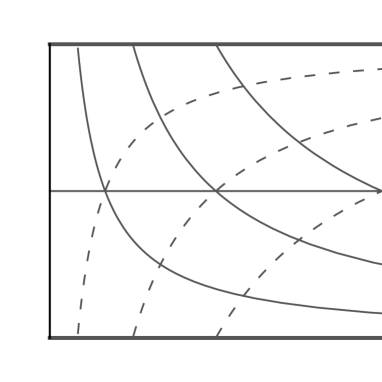
Figure 1: Panel (a) shows a coordinate diagram with the cylinder at spatial infinity for the Minkowski spacetime. Panel (b) shows the Penrose diagram of the Minkowski spacetime with the lightcone at the origin is depicted in light-gray: the region where the $F$-coordinates are valid is the complement of this cone (neighbourhood of $i^{0}$). The continuous lines represent null surfaces $\tilde{u}=-|\tilde{u}_{\star}|$ the dashed ones represent null surfaces $\tilde{v}=|\tilde{v}_{\star}|$.

Exploiting Remark 4 it is clear how to identify initial data for the physical good field which leads to log-free expansions. Splitting the initial data for $\dot{\phi}$ as

$$\dot{\phi}|_{\mathcal{S}}=\sum_{p=0}^{\infty}\sum_{m=-p}^{m=p}\frac{1}{p!}\dot{a}_{p;p,m}(0)Y_{\ell m}\rho^{p}+\sum_{p=1}^{\infty}\;\;\sum_{\ell=1}^{\max\{1,\;p-1\}}\sum_{m=-\ell}^{m=\ell}\frac{1}{p!}\dot{a}_{p;\ell,m}(0)Y_{\ell m}\rho^{p},$$ (48)

then it follows that to have a log-free expansion at all orders one needs special initial data of the form

$$\dot{\phi}|_{\mathcal{S}}=\sum_{p=1}^{\infty}\;\;\sum_{\ell=1}^{{\max\{1,\;p-1\}}}\sum_{m=-\ell}^{m=\ell}\frac{1}{p!}\dot{a}_{p;\ell,m}(0)Y_{\ell m}\rho^{p}.$$ (49)

Remark 7.

Notice also that the appearance of the logs is irrespective of the value of $a_{p,\ell,m}(0)$ and hence of the initial data for $\phi|_{\mathcal{S}}$ as given in equation (36). Using Proposition 1 one has that $\partial_{\tau}\phi|_{\mathcal{S}}=\tilde{\rho}\partial_{\tilde{t}}\phi|_{\mathcal{S}}$. Hence, recalling that $\phi=\Theta^{-1}\tilde{\phi}$, then $\dot{\phi}|_{\mathcal{S}}=\tilde{\rho}^{2}\partial_{\tilde{t}}\tilde{\phi}|_{\mathcal{S}}$.

This leads to the following

Proposition 3.

Initial data for the physical good field satisfying

$$\tilde{\phi}|_{\mathcal{S}}=\sum_{p=0}^{\infty}\sum_{\ell=0}^{p}\sum_{m=-\ell}^{m=\ell}\frac{1}{p!}a_{p;\ell,m}(0)Y_{\ell m}\tilde{\rho}^{p-1},\quad\partial_{\tilde{t}}\tilde{\phi}|_{\mathcal{S}}=\sum_{p=1}^{\infty}\sum_{\ell=1}^{{\max\{1,\;p-1\}}}\sum_{m=-\ell}^{m=\ell}\frac{1}{p!}\dot{a}_{p;\ell,m}(0)Y_{\ell m}\tilde{\rho}^{-p-2}.$$ (50)

gives rise to a log-free expansion close to $I$.

If one is only interested in suppressing the leading logarithm —that associated to $D_{000}$— then requiring that the initial data for the physical good field satisfies

$$\partial_{\tilde{t}}\tilde{\phi}|_{\mathcal{S}}=\mathcal{O}(\tilde{\rho}^{-3})$$ (51)

ensures that $D_{000}=0$. Later it will be shown that the condition (51), is sufficient but not necessary to do so. Moreover, it does not prevent the appearance of higher order logs.

3.2 The ugly equation

It was observed in [12] that the simple linear wave equation 30c, motivated by the equation of motion for certain components of the physical metric in generalised harmonic gauge, gives rise to polyhomogeneous expansions near null infinity. Using the identity (31) and the specific feature of the $i^{0}$-cylinder background discussed in Section 2, one gets

$$\square\phi =\frac{2}{\tilde{\rho}}\Theta^{-3}\tilde{\nabla}_{\tilde{t}}\tilde{\phi}$$

$$=2\Theta^{-1}\tilde{\nabla}_{\tilde{t}}(\Theta^{-1}\tilde{\phi})$$

$$=(\kappa\nabla_{\underline{\ell}}\phi+\kappa^{-1}\nabla_{\ell}\phi)$$ (52)

where from the first to the second line equation (28) was employed.

Remark 8.

Although it may appear obvious that the conformal factor $\Theta$ is a function of the physical radial coordinate $\tilde{\rho}$ only, this fact is not assumed a priori in the general framework of the conformal Einstein field equations. In the case of the Minkowski spacetime the relation between the physical and unphysical coordinates is explicitly known so that this relation be given in closed form.

Observe as well that although the unphysical ugly equation

$$\square\phi =\kappa\nabla_{\underline{\ell}}\phi+\kappa^{-1}\nabla_{\ell}\phi$$ (53)

does not contain any $\Theta^{-1}$ term, the boost parameter $\kappa$ and its inverse appear in equation (53) which is singular at $\tau=\pm 1$ respectively. The unphysical ugly equation in the $F$-coordinates reads

$$(\tau^{2}-1)\partial_{\tau}^{2}\phi-2\rho\tau\partial_{\tau}\partial_{\rho}\phi+\rho^{2}\partial_{\rho}^{2}\phi+2(\tau+q)\partial_{\tau}\phi+4\rho\tau(\tau^{2}-1)^{-1}\partial_{\rho}\phi+\Delta_{\mathbb{S}^{2}{}}{}\phi=0.$$ (54)

Using the Ansatz of equation (34) then renders the following ODE for $a_{p;\ell,m}$

$$(1-\tau^{2})\ddot{a}_{p;\ell,m}+2(\tau(p-1)-1)\dot{a}_{p,\ell,m}+\Big{[}(\ell+p)(\ell-p+1)+\frac{p\tau}{1-\tau^{2}}\Big{]}{a}_{p;\ell,m}=0.$$ (55)

Similarly to equation (33), this equation is formally singular at $\tau=\pm 1$, hence to contrast equations (33) and (55), the latter can be written more fairly if we multiply through by $1-\tau^{2}$

$$(1-\tau^{2})^{2}\ddot{a}_{p;\ell,m}+2(1-\tau^{2})(\tau(p-1)-1)\dot{a}_{p,\ell,m}+\Big{[}(\ell+p)(\ell-p+1)(1-\tau^{2})+p\tau\Big{]}{a}_{p;\ell,m}=0.$$ (56)

Unfortunately, equation (56) does not have the form of a Jacobi equation in which the theory of special functions of [34] can be applied. Presumably, (56) lies in the class of the Heun equation and could be solved accordingly in terms of special functions and power series. Although the latter described strategy could be pursued, an alternative, cleaner, approach is to realise that the ugly model equation can be written as a good equation for a suitably defined field and then apply the analysis of subsection 3.1 on this newly defined field. To do so it is convenient to rewrite it in terms of null directions. The physical ugly equation (30c) expressed using the physical outgoing and incoming null vectors reads

$$\tilde{\square}\tilde{\phi}-\frac{1}{\tilde{\rho}}(L\tilde{\phi}+\underline{L}\tilde{\phi})=0.$$ (57)

Using that $\tilde{\square}$ can be written in terms of $L$ and $\underline{L}$ as

$$\tilde{\square}\tilde{\phi}:=-\frac{1}{\tilde{\rho}}L\underline{L}(\tilde{\rho}\tilde{\phi})+\frac{1}{\tilde{\rho^{2}}}\Delta_{\mathbb{S}^{2}}\tilde{\phi},$$ (58)

and using the expressions for $L$ and $\underline{L}$ as given in equation (23), the following ‘commutation relation’ can be derived

$$\underline{L}(\tilde{\rho}^{2}\tilde{\square}\tilde{\phi})-\tilde{\rho}\tilde{\square}(\tilde{\rho}\underline{L}\tilde{\phi})=\underline{L}(\tilde{\rho}(L+\underline{L})\tilde{\phi}).$$ (59)

The latter expression can be rewritten as

$$\underline{L}\Bigg{(}\tilde{\rho}^{2}\Big{(}\tilde{\square}\tilde{\phi}-\frac{1}{\tilde{\rho}}(L\tilde{\phi}+\underline{L}\tilde{\phi})\Big{)}\Bigg{)}=\tilde{\rho}\tilde{\square}(\tilde{\rho}\underline{L}\tilde{\phi}).$$ (60)

Hence, the physical ugly equation (57) implies that

$$\tilde{\square}\tilde{\Phi}=0.$$ (61)

where

$$\tilde{\Phi}=\tilde{\rho}\underline{L}\tilde{\phi}.$$ (62)

The initial data for the auxiliary problem (61) is not free if the aim is to construct a solution to the physical ugly equation (57). To see this, notice that from equation (60) it follows that by solving the auxiliary problem (61) and (62), one is not necessarily obtaining a solution to the ugly equation (57), but rather to the more general equation

$$\tilde{\square}\tilde{\phi}-\frac{1}{\tilde{\rho}}(L\tilde{\phi}+\underline{L}\tilde{\phi})=Q,$$ (63)

where $Q$ is smooth function of the physical coordinates $\tilde{x}^{\mu}$ that satisfies $\underline{L}(\tilde{\rho}^{2}Q)=0$. The source term $Q$ encodes the relation between the data for the physical ugly field $\tilde{\phi}$ and the auxiliary physical good field $\tilde{\Phi}$. To clarify this relation observe that using equation (62) and writing equation (63) as

$$-\partial_{\tilde{t}}^{2}\tilde{\phi}+\Delta\tilde{\phi}+\frac{2}{\tilde{\rho}}\partial_{\tilde{t}}\tilde{\phi}=Q,$$ (64)

where $\Delta$ denotes the Laplace operator of 3-dimensional Euclidean space, it follows that the initial data is related via

$$\tilde{\Phi}|_{\mathcal{S}} =\left[\tilde{\rho}(\partial_{\tilde{t}}-\partial_{\tilde{\rho}})\tilde{\phi}\right]_{\mathcal{S}},$$ (65a)

$$\partial_{\tilde{t}}\tilde{\Phi}|_{\mathcal{S}} =\left[\tilde{\rho}(\partial^{2}_{\tilde{t}}-\partial_{\tilde{\rho}}\partial_{\tilde{t}})\tilde{\phi}\right]_{\mathcal{S}}=\left[\tilde{\rho}(\Delta\tilde{\phi}+2\tilde{\rho}^{-1}\partial_{\tilde{t}}\tilde{\phi}-Q-\partial_{\tilde{\rho}}\partial_{\tilde{t}}\tilde{\phi})\right]_{\mathcal{S}}$$ (65b)

Once the appropriate initial data for the auxiliary field $\tilde{\Phi}$ has been obtained, then using that $\underline{L}=2\partial_{\tilde{u}}$, integrating the expression (62) along the incoming null geodesic, one gets the formal expression

$$\tilde{\phi}=\frac{1}{2}\int_{\tilde{u}_{\star}}^{\tilde{u}}\frac{\tilde{\Phi}(\bar{u},\tilde{v})}{\tilde{\rho}(\bar{u},\tilde{v})}d\bar{u}.$$ (66)

Hence, the analysis for the physical good equation given in subsection 3.1.2 and summarised in Proposition 2 provides a general solution to the auxiliary problem —modulo adjusting the initial data as describe before. Multiplying by $\/\tilde{\rho}$ and integrating the asymptotic expansion for the physical good field given in Lemma 2, one obtains

$$\tilde{\phi}= \int_{\tilde{u}_{\star}}^{\tilde{u}}\Big{\{}\frac{C_{000}Y_{00}}{\tilde{\rho}^{2}}+\frac{Y_{00}}{2\tilde{\rho}^{2}}\Big{(}\frac{A_{100}}{\tilde{v}}-\frac{B_{100}}{\bar{u}}+D_{000}\log\kappa\Big{)}+\frac{C_{11-1}Y_{1-1}+C_{111}Y_{11}+C_{110}Y_{10}}{4\tilde{\rho}^{3}}$$

$$+\frac{1}{32\tilde{\rho}^{3}}\Big{(}\frac{\bar{u}}{\tilde{v}}-\frac{\tilde{v}}{\bar{u}}+2\log\kappa\Big{)}(D_{11-1}Y_{1-1}+D_{110}Y_{10}+D_{111}Y_{11})+\mathcal{O}(\tilde{\rho}^{-4})\Big{\}}d\bar{u}.$$

which, after integration renders,

$$\tilde{\phi}= \frac{2C_{000}Y_{00}}{\tilde{\rho}}+\frac{Y_{00}(A_{100}-B_{100})}{\tilde{v}\tilde{\rho}}-\frac{2B_{100}Y_{00}}{\tilde{v}^{2}}\log\Big{(}-\frac{\tilde{u}}{2\tilde{\rho}}\Big{)}+\frac{Y_{00}D_{000}\log\kappa}{\tilde{\rho}}$$

$$+\frac{2D_{000}Y_{00}}{\tilde{v}}\log\Big{(}-\frac{\tilde{u}}{2\tilde{\rho}}\Big{)}+\frac{C_{11-1}Y_{1-1}+C_{111}Y_{11}+C_{110}Y_{10}}{4\tilde{\rho}^{2}}-\frac{D_{11-1}Y_{1-1}+D_{110}Y_{10}+D_{111}Y_{11}}{8\tilde{v}\tilde{\rho}}$$

$$+\frac{D_{11-1}Y_{1-1}+D_{110}Y_{10}+D_{111}Y_{11}}{16\tilde{\rho}^{2}}\log\kappa+\mathcal{O}(\tilde{\rho}^{-3}).$$ (67)

Remark 9.

The term $\log(-\frac{\tilde{u}}{2\tilde{\rho}})$ is a real valued function since the range of validity of the inversion unphysical coordinates $x^{\mu}$ in equation (3) —used in turn to build the $F$-coordinates— correspond to the region determined by $\tilde{\rho}>0$ with $\tilde{u}<0$ and $\tilde{v}>0$.

Remark 10.

Observe that there are two types of logarithmic terms appearing in the expression (3.2), those coming from integration of terms such as $\tilde{\rho}^{-1}\tilde{u}^{-1}$ and those inherited from the terms containing $\log\kappa$ in the good field. The logs reported in [12] can only correspond to the former since in the last reference the good field does not contain any logarithmic term.

Choosing initial data for the auxiliary good field ensuring $Q=0$ within the working Ansatz (34) boils down to setting to zero some of the constants in equation (36). To the order shown in equation (3.2) this corresponds to setting $A_{100}=D_{000}=D_{110}=D_{111}=D_{11-1}=0$ which in particular gets rid of all the logarithmic terms directly inherited from the good field. The last discussion is summarised in the following

Proposition 4.

Let $\tilde{\phi}_{u}$ be a solution to equation (30c) constructed from solving equations (61) and (62) with analytic initial data close to $I$. Then, the field $\tilde{\phi}_{u}$ has the following asymptotic expansion near $I$:

$$\tilde{\phi}_{u}= \frac{2C_{000}Y_{00}}{\tilde{\rho}}-\frac{Y_{00}B_{100}}{\tilde{v}\tilde{\rho}}-\frac{2B_{100}Y_{00}}{\tilde{v}^{2}}\log\Big{(}-\frac{\tilde{u}}{2\tilde{\rho}}\Big{)}+\frac{C_{11-1}Y_{1-1}+C_{111}Y_{11}+C_{110}Y_{10}}{4\tilde{\rho}^{2}}+\mathcal{O}(\tilde{\rho}^{-3}).$$ (68)

3.3 The bad equation

Using the identity (31) and substituting the physical bad equation (30b), one gets

$$\square\phi_{b} =\Theta^{-3}(\tilde{\nabla}_{\tilde{t}}\tilde{\phi}_{g})^{2},$$

$$=\Theta^{-1}(\tilde{\nabla}_{\tilde{t}}\phi_{g})^{2},$$

$$=\frac{1}{4}\Theta(\kappa\nabla_{\underline{\ell}}\phi_{g}+\kappa^{-1}\nabla_{\ell}\phi_{g})^{2},$$ (69)

where from the first to the second line equation (28) was employed. From the second to the third line, the relation between the physical and unphysical fields $\tilde{\phi}=\Theta\phi$ and the results of Proposition 1 were used. Notice that, similarly to the case of the ugly equation, although there are no singular terms of the form $\Theta^{-1}$, the unphysical bad equation

$$\square\phi_{b}=\frac{1}{4}\Theta(\kappa\nabla_{\underline{\ell}}\phi_{g}+\kappa^{-1}\nabla_{\ell}\phi_{g})^{2},$$ (70)

does contain terms which will be singular at $\mathscr{I}^{+}$ and $\mathscr{I}^{-}$, due to the presence of the boost parameter in the form $\Theta\kappa^{2}$ and $\Theta\kappa^{-2}$, respectively. Given that the good and bad fields are decoupled, the analysis of the bad equation follows as a sub-case of the analysis of the following wave equation with sources

$$\square\phi=f$$ (71)

where $f=f(\tau,\rho,\theta^{A})$. Proceeding as before, using the Ansatz (34), the calculation boils down to analysing the ODE:

$$(1-\tau^{2})\ddot{a}_{p;\ell,m}+2\tau(p-1)\dot{a}_{p,\ell,m}+(\ell+p)(\ell-p+1){a}_{p;\ell,m}=f_{p;\ell,m}(\tau).$$ (72)

where $f_{p;\ell,m}(\tau)$ arises from expanding $f$ according to the Ansatz (34). The analysis of this wave equation has been given in Appendix D of [29] which we recall here:

Lemma 2 (Inhomogeneous wave equation on the $i^{0}$-cylinder background [29]).

The solution $a_{p;\ell,m}(\tau)$ of equation (72) can be written as:

$$a_{p;\ell,m}(\tau)=a^{H}_{1:p;\ell,m}(\tau)b_{1:p;\ell,m}(\tau)+a^{H}_{2:p;\ell,m}(\tau)b_{2:p;\ell,m}(\tau),$$ (73)

where $a^{H}_{1:p;\ell,m}(\tau)$ and $a^{H}_{2:p,\ell,m}(\tau)$ are two independent solutions to the homogeneous problem —namely, with $f(\tau)=0$— while $b_{1:p;\ell,m}(\tau)$ and $b_{2:p;\ell,m}(\tau)$ are given by

$$b_{1:p;\ell,m}(\tau)=F_{p;\ell,m}-\int_{0}^{\tau}\frac{a_{2:p;\ell,m}(s)f_{p,\ell,m}(s)}{W_{\star}(1-s^{2})^{p}}ds,$$ (74a)

$$b_{2:p,\ell,m}(\tau)=G_{p;\ell,m}-\int_{0}^{\tau}\frac{a_{1:p;\ell,m}(s)f_{p,\ell,m}(s)}{W_{\star}(1-s^{2})^{p}}ds.$$ (74b)

where $F_{p;\ell,m}$, $G_{p;\ell,m}$ and $W_{\star}$ are constants.

Naturally, the behaviour of the solution $a(\tau)$ hence depends on the regularity of the source $f(\tau)$. In the case of the bad equation (70) the source term is given by

$$f=\frac{1}{4}\Theta(\kappa\nabla_{\underline{\ell}}\phi_{g}+\kappa^{-1}\nabla_{\ell}\phi_{g})^{2}$$ (75)

where $\phi_{g}$ is the solution to equation (32), hence, in principle, $f(\tau)$ could contain both poles at $\tau=\pm 1$ and logarithmic terms of the form $\log(1\pm\tau)$. More explicitly, the source reads

$$f=-\frac{\rho}{1-\tau^{2}}((1-\tau^{2})\partial_{\tau}\phi_{g}+2\rho\tau\partial_{\rho}\phi_{g})^{2}.$$ (76)

A first observation is that the logarithmic terms coming from $\phi_{g}$ do not give rise to logarithmic terms in the source $f$ since

$$\partial_{\tilde{t}}\log\kappa=\frac{1}{2}(\partial_{\tilde{u}}+\partial_{\tilde{v}})\log\kappa=-\frac{1}{2}\Big{(}\frac{1}{\tilde{u}}-\frac{1}{\tilde{v}}\Big{)}.$$ (77)

A direct calculation using the solutions for the unphysical good field $\phi_{g}$ as determined by Lemma 1 gives:

$$f= \frac{\rho D_{000}{}^{2}Y_{00}{}^{2}}{1-\tau^{2}}+\frac{\rho^{2}D_{000}Y_{00}}{2(1-\tau^{2})}\Big{(}D_{11-1}Y_{1-1}+D_{110}Y_{10}+D_{111}Y_{11}-2A_{100}Y_{00}(1-\tau)^{2}$$

$$+2B_{100}Y_{00}(1+\tau)^{2}\Big{)}+\mathcal{O}(\tilde{\rho}^{-3}).$$ (78)

In general, $f$ will contain products of spherical harmonics, hence, to extract $f_{p;\ell,m}(\tau)$ one would need to express $Y_{\ell,m}Y_{{\ell^{\prime}},{m^{\prime}}}$ in terms of linear combinations of $Y_{L,M}$ where $|\ell-\ell^{\prime}|\leq L\leq\ell+\ell^{\prime}$ and $M=m+m^{\prime}$, via the Clebsch-Gordan coefficients. Fortunately, to the pursued order, this will not be necessary since one of the factors is $Y_{00}$, which is constant. Using equation (3.3), along with Lemmas 1 and 2, gives the following expansion for the unphysical bad field $\phi_{b}$

$$\phi_{b}=C_{000}F_{000}Y_{00}+\tfrac{1}{2}G_{000}\log(\kappa)Y_{00}+\rho(H_{1}+H_{2}\tau+H_{3}\tau^{2}+\log\kappa(H_{4}+H_{5}\tau^{2}))+\mathcal{O}(\rho^{2}),$$ (79)

where,

$$H_{1} =\frac{1}{2}(A_{100}F_{100}+B_{100}G_{100})Y_{00}+\frac{1}{4}(C_{11-1}F_{11-1}Y_{1-1}+C_{110}F_{110}Y_{10}+C_{111}F_{111}Y_{11}),$$

$$H_{2} =-\frac{Y_{00}}{8\pi^{1/2}W_{*}{}}\Big{(}A_{100}(B_{100}D_{000}{}^{2}+4\pi^{1/2}W_{*}{}F_{100})-4\pi^{1/2}W_{*}{}B_{100}G_{100}\Big{)}$$

$$\quad+\frac{1}{8}(G_{11-1}Y_{1-1}+G_{110}Y_{10}+G_{111}Y_{11}),$$

$$H_{3} =-\frac{1}{4}(C_{11-1}F_{11-1}Y_{1-1}+C_{110}F_{110}Y_{10}+C_{111}F_{111}Y_{11}),$$

$$H_{4} =\frac{1}{16}\Big{(}-\frac{A_{100}B_{100}D_{000}{}^{2}Y_{00}}{\pi^{1/2}W_{*}{}}+G_{11-1}Y_{1-1}+G_{110}Y_{10}+G_{111}Y_{11}\Big{)},$$

$$H_{5} =-\frac{1}{16}\Big{(}G_{11-1}Y_{1-1}+G_{110}Y_{10}+G_{111}Y_{11}\Big{)}.$$ (80)

To obtain the physical bad field it is enough to recall that $\tilde{\phi}=\Theta\phi$ and rewrite equation (79) in terms of the physical coordinates. A calculation then reveals the following:

Proposition 5.

The solution $\tilde{\phi}_{b}$ to equation (30a) —the physical bad equation— arising from analytic initial data close to the cylinder at spatial infinity $I$ has the following formal expansion

$$\tilde{\phi}_{b}= \frac{A_{100}B_{100}D_{000}{}^{2}\log(\kappa)Y_{00}}{16\pi^{1/2}W_{*}{}\tilde{v}\tilde{u}}+\frac{1}{\tilde{\rho}}\Big{(}C_{000}F_{000}Y_{00}+\tfrac{1}{2}G_{000}\log(\kappa)Y_{00}$$

$$+\frac{A_{100}(B_{100}D_{000}{}^{2}+8\pi^{1/2}W_{*}{}F_{100})Y_{00}}{16\pi^{1/2}W_{*}{}\tilde{v}}+\frac{B_{100}(A_{100}D_{000}{}^{2}-8\pi^{1/2}W_{*}{}G_{100})Y_{00}}{16\pi^{1/2}W_{*}{}\tilde{u}}\Big{)}$$

$$\frac{1}{\tilde{\rho}^{2}}\Big{(}C_{11-1}F_{11-1}Y_{1-1}+C_{110}F_{110}Y_{10}+C_{111}F_{111}Y_{11}\Big{)}$$

$$+\frac{1}{32\tilde{\rho}^{2}}\Big{(}\frac{\tilde{u}}{\tilde{v}}+2\log\kappa-\frac{\tilde{v}}{\tilde{u}}\Big{)}(C_{11-1}F_{11-1}Y_{1-1}+C_{110}F_{110}Y_{10}+C_{111}F_{111}Y_{11})+\mathcal{O}(\tilde{\rho}^{-3})$$ (81)

3.4 Comparison with the higher-order asymptotic expansion

The most clean case to compare the logs obtained in [12] and those appearing through the analysis of the cylinder at spatial infinity is that of the good field: on the one hand, the asymptotic expansion for the good field $\tilde{\phi}_{g}$ reported in [12] does not contain log terms while the solution of Proposition 2 contains logs. However, to go beyond this obvious observation and to make a comparison in a more equal footing it is necessary to recall that the expansions in [12] are obtained through integration along outgoing null directions and the parameter along this curve was chosen to be the physical radial coordinate $\tilde{\rho}$. Therefore to put the expansion (2) in the same format, one needs to evaluate it at a fiduciary retarded time

$$\tilde{u}=-|\tilde{u}_{\star}|.$$ (82)

Hence on these surfaces one has

$$\tilde{v}=-|\tilde{u}_{\star}|+2\tilde{\rho},$$ (83)

where $\tilde{\rho}>|\tilde{u}_{\star}|/2$ so that $\tilde{v}>0$ and $\tilde{u}<0$. Then, substituting expressions (82) and (83) in the expansion (2) one obtains, after Taylor expanding close to the associated cut of null infinity $\mathcal{C}_{\star}\subset\mathscr{I}$, the following expression:

$$\tilde{\phi}_{g}= \frac{C_{000}Y_{00}}{\tilde{\rho}}+\frac{1}{16|\tilde{u}_{\star}|\tilde{\rho}}\Big{(}8B_{100}Y_{00}+D_{11-1}Y_{1-1}+D_{110}Y_{10}+D_{111}Y_{11}\Big{)}+\frac{D_{000}Y_{00}}{2\tilde{\rho}}\log\bigg{(}\frac{2\tilde{\rho}}{|\tilde{u}_{\star}|}\bigg{)}$$

$$+ \frac{1}{32\tilde{\rho}^{2}}\Big{(}8(A_{100}-|\tilde{u}_{\star}|D_{000})+(8C_{11-1}-D_{11-1})Y_{1-1}+(8C_{110}-D_{110})Y_{10}+(8C_{111}-D_{111})Y_{11}\Big{)}$$

$$+ \frac{1}{16\tilde{\rho}^{2}}\log\bigg{(}\frac{2\tilde{\rho}}{|\tilde{u}_{\star}|}\bigg{)}(D_{11-1}Y_{1-1}+D_{110}Y_{10}+D_{111}Y_{11})+\mathcal{O}(\tilde{\rho}^{-3}\log{\tilde{\rho}}).$$ (84)

Remark 11.

The last expression contains terms proportional to $\log(\tilde{\rho})$ for any finite $\tilde{u}_{\star}\neq 0$. In contrast, the expression for the good field reported in [12] does not contain these logs. Naturally, choosing initial data so that $D_{p;\ell,m}=0$ (the data for $\dot{a}_{p;p,m}(0)$, see Remark 4) one recovers a log-free expansion —see Proposition 3.

Similarly, for the ugly field, using equations (82) and (83) on the expansion (68) gives:

$$\tilde{\phi}_{u}=\frac{2C_{000}Y_{00}}{\tilde{\rho}}+\frac{-2B_{100}Y_{00}+C_{11-1}Y_{1-1}+C_{110}Y_{10}+C_{111}Y_{11}}{4\tilde{\rho}^{2}}-\frac{B_{100}Y_{00}}{2\tilde{\rho}^{2}}\log\bigg{(}\frac{|\tilde{u}_{\star}|}{2\tilde{\rho}}\bigg{)}+\mathcal{O}(\tilde{\rho}^{-3}\log\tilde{\rho}).$$ (85)

Remark 12.

To this order, the last expansion agrees with the general form expected for the expansion of the ugly field as given in [12] since $\log\tilde{\rho}$ starts from the second order in $\tilde{\rho}$. Observe that the potential logs inherited from the good field —and directly related to the $i^{0}$-cylinder framework— appearing equation (3.2) get removed after imposing initial data ensuring $Q=0$ within the working Ansatz (34) —see Remark 10. Hence, unlike the case of the good and bad fields where both contributions are present, the logs in (85) correspond exclusively to those reported in [12].

Finally, proceeding analogously with the bad field using equation (5), one obtains:

$$\tilde{\phi}_{b}= \frac{1}{\tilde{\rho}}\Big{[}C_{000}F_{000}Y_{00}-\frac{A_{100}B_{100}D_{000}{}^{2}Y_{00}}{16\pi^{1/2}W_{*}|\tilde{u}_{*}{}|}$$

$$\quad-\frac{1}{16|\tilde{u}_{*}{}|}(8B_{100}G_{100}Y_{00}+G_{11-1}Y_{1-1}+G_{110}Y_{10}+G_{111}Y_{11})\Big{]}$$

$$+\frac{1}{64\tilde{\rho}^{2}}\Big{[}\frac{A_{100}(3B_{100}D_{000}{}^{2}+16\pi^{1/2}W_{*}{}F_{100})-16\pi^{1/2}|\tilde{u}_{*}{}|W_{*}{}G_{000})Y_{00}}{\pi^{1/2}W_{*}{}}$$

$$\qquad\quad+2((8C_{11-1}F_{11-1}-G_{11-1})Y_{1-1}+(8C_{110}F_{110}-G_{110})Y_{10}+(8C_{111}F_{111}-G_{111})Y_{11})\Big{]}$$

$$+\frac{1}{64\pi^{1/2}W_{*}}\log\Big{(}\frac{2\tilde{\rho}}{|\tilde{u}_{\star}|}\Big{)}\Big{[}\frac{2(-A_{100}B_{100}D_{000}{}^{2}+16\pi^{1/2}|\tilde{u}_{*}{}|W_{*}{}G_{000})Y_{00}}{|\tilde{u}_{*}{}|\tilde{\rho}}$$

$$\qquad\qquad-\frac{A_{100}B_{100}D_{000}{}^{2}Y_{00}-4\pi^{1/2}W_{*}(G_{11-1}Y_{1-1}+G_{110}Y_{10}+G_{111}Y_{11})}{\tilde{\rho}^{2}}\Big{]}+\mathcal{O}(\tilde{\rho}^{-3}\log\tilde{\rho})$$ (86)

Remark 13.

The $\log\tilde{\rho}$ terms in the last expression agree with the general form expected for the bad field according to [12]. Nevertheless, the logarithmic terms in expression (3.4) have two types of contributions: one contribution comes from the logs present in the expansion of the good field —with initial data $D_{p;\ell,m}\neq 0$— and the other comes from terms which are present even for a log-free expansion of the good field —with initial data $D_{p;\ell,m}=0$.

A reevaluation of the asymptotic system analysis to understand the apparent discrepancies is given in section 3.5.

3.5 Revisiting the asymptotic system

The analysis of the previous section shows that the logarithmic terms discussed in [12] are not in correspondence with the logarithmic terms having origin at spatial infinity using the $i^{0}$-cylinder framework. Since this discrepancy is more cleanly shown by the expansion of the good field —one method apparently renders log-free expansions while the other does not— it is of interest to revisit the asymptotic approximation upon which the expansions of [12] were derived —namely Hörmander’s asymptotic system— under the light of Proposition 2.

Hörmander’s asymptotic system is based on the observation that derivatives tangent to the outgoing null cone decay faster than transverse derivatives to it. This leads to calling $\underline{L}$ the bad derivative and, along with angular derivatives, calling $L$ the good derivative. The first order asymptotic system for the wave equation is based on the heuristic approach of disregarding the terms that only contain good derivatives. Expressing the physical wave operator in Minkowski spacetime as in equation (58), discarding the second term as it only contains two good —angular— derivatives, one obtains

$$L\underline{L}(\tilde{\rho}\tilde{\phi})\simeq 0$$ (87)

where the symbol $\simeq$ is used to emphasise that the previously described asymptotic approximation has been used. The last expression can be integrated as follows

$$\partial_{\tilde{u}}\partial_{\tilde{v}}(\tilde{\rho}\tilde{\phi})\simeq \;0,$$

$$\partial_{\tilde{v}}(\tilde{\rho}\tilde{\phi})\simeq (\partial_{\tilde{v}}(\tilde{\rho}\tilde{\phi}))|_{\tilde{u}_{\star}}:=f(\tilde{v},\theta^{A}),$$

$$\tilde{\rho}\tilde{\phi}\simeq (\tilde{\rho}\tilde{\phi})|_{\tilde{v}_{\star}}+\int_{\tilde{v}_{\star}}^{\tilde{v}}f(\bar{v},\theta^{A})d\bar{v},$$

$$\implies\tilde{\phi}\simeq \frac{1}{\tilde{\rho}}(G(\tilde{u},\theta^{A})+F(\tilde{v},\theta^{A})),$$ (88)

where in this calculation $f$ appears as an “integration constant” determined from given data for $\partial_{\tilde{v}}(\tilde{\rho}\tilde{\phi})$ and $G(\tilde{u},\theta^{A})$ is an “integration constant” resulting from data for $\tilde{\rho}\tilde{\phi}$. Similarly the function $F(\tilde{v},\theta^{A})$ is a shorthand for $\int_{\tilde{v}}f$ appearing in the third line of the derivation of expression (3.5). Therefore, this approach can serve as the foundation of a heuristic method for determining the general form of the field in general asymptotically flat backgrounds as was done in [12]. Nonetheless, observe that the functional form of $F(\tilde{v},\theta^{A})$ and $G(\tilde{u},\theta^{A})$ is not given explicitly by the method and are determined implicitly by initial data, given for instance on $\mathcal{S}$ when one considers the Cauchy problem. Hence, $F(\tilde{v},\theta^{A})$ and $G(\tilde{u},\theta^{A})$ can accommodate for the logarithmic terms appearing in Proposition 2. In other words, the logarithmic terms arising from the critical sets are, in some sense, not missed by the asymptotic system heuristics as they are contained inside the “integration constants”. However, the asymptotic system method by itself does not give information on the functional form of these “integration constants” or the field itself at the critical sets where spatial and null infinity meet. Nonetheless, one can still retrieve the first order logarithmic term appearing in the good field by means of the leading order asymptotic system heuristics. To do so notice that if initial data is chosen so that

$$f(\tilde{v},\theta^{A})\simeq\tilde{v}^{-1}M(\theta^{A})+o(\tilde{v}^{-1}),$$ (89)

where $M$ is a function of $\theta^{A}$ and the standard little-o notation is used in the second term, then integrating the second line in equation (3.5) gives

$$\tilde{\phi}\simeq\frac{\log\tilde{v}}{\tilde{\rho}}M(\theta^{A})+\frac{1}{\tilde{\rho}}G(\tilde{u},\theta^{A}),$$ (90)

Then, on outgoing null directions $u=u_{\star}$ one recovers

$$\tilde{\phi}\simeq\frac{\log\tilde{\rho}}{\tilde{\rho}}M(\theta^{A})+\frac{1}{\tilde{\rho}}G(\tilde{u},\theta^{A}),$$ (91)

Notice that these logarithmic terms were discarded in the analysis of [12]. Additionally, observe that the condition ensuring the absence of the leading logarithmic term is

$$f(\tilde{v},\theta^{A})\simeq\mathcal{O}(\tilde{v}^{-2}).$$ (92)

A attractive feature of expressing the “no-leading-order-log condition” in terms of (92) is that it allows for a simple physical interpretation: if the initial data for the incoming characteristic variable $\partial_{\tilde{v}}(\tilde{\rho}\tilde{\phi})$ decays faster than $\mathcal{O}(\tilde{v}^{-1})$, then there will be no leading log-term in the solution for $\tilde{\phi}$ towards $\mathscr{I}^{+}$. On the other hand, the analysis using the $i^{0}$-cylinder predicts a hierarchy of logarithmic terms in the expansion for the good field. The first order logarithmic term obtained through the conformal approach is controlled at the level of initial data by the coefficient $D_{000}$ —higher order logs being controlled by $D_{n,n,m}$ with $n\geq 1$. Thus, verifying that the asymptotic system heuristics described above capture the leading log-term predicted by the $i^{0}$-cylinder method one needs to check their correspondence at the level of initial data. To do so, observe that

$$f(\tilde{v},\theta):=(\partial_{\tilde{v}}(\tilde{\rho}\tilde{\phi}))|_{\tilde{u}_{\star}}=\big{(}\partial_{\tilde{t}}(\tilde{\rho}\tilde{\phi})+\partial_{\tilde{\rho}}(\tilde{\rho}\tilde{\phi})\big{)}|_{\mathcal{S}},$$ (93)

thus, assuming that the initial data has a series expansion in integer powers of $\tilde{\rho}^{-1}$, a necessary and sufficient condition to get rid of the leading log at null infinity from the point of view of the asymptotic system heuristics is that

$$\big{(}\partial_{\tilde{t}}(\tilde{\rho}\tilde{\phi})+\partial_{\tilde{\rho}}(\tilde{\rho}\tilde{\phi})\big{)}|_{\mathcal{S}}\sim\mathcal{O}(\tilde{\rho}^{-2}),$$ (94)

where to re-express (92) it was used that on $u=u_{\star}$ one has $\tilde{v}\sim\tilde{\rho}$. Rewriting the condition (94) in terms of the unphysical fields, using the results from Proposition 1 —as similarly done in Remark (7)— and substituting the initial data Ansatz (36), one gets

$$\big{(}\partial_{\tilde{t}}(\tilde{\rho}\tilde{\phi})+\partial_{\tilde{\rho}}(\tilde{\rho}\tilde{\phi})\big{)}|_{\mathcal{S}}\simeq\frac{1}{\tilde{\rho}}D_{000}+\mathcal{O}(\tilde{\rho}^{-2}).$$ (95)

Hence the no-leading-log condition $D_{000}=0$ obtained from the $i^{0}$-cylinder analysis corresponds precisely to the condition (94) expressed in the physical picture. Therefore, one can conclude that the leading log obtained through the above described method based on the asymptotic system retrieves the first order log obtained through the $i^{0}$-cylinder analysis. Notice however that the leading log corresponds to the spherically symmetric solution (terms with $Y_{00}$) while the higher order logs are related to a specific harmonics in the Ansatz (34) —associated to non-trivial spherical harmonics $Y_{\ell m}$. Obtaining a generalisation of the present new take on the asymptotic system heuristics to higher order is left for future work.

Choosing initial data of compact support all log-terms are of course suppressed. The foregoing discussion shows that the first order asymptotic system captures the case in which log-terms are absent in the initial data but manifest at future null infinity. But one furthermore observes from the general solution to the asymptotic system (3.5) that examples in which log-terms appear in the initial data, but not at future null infinity are easily constructed (mutatis mutandis at past null infinity). For instance, one may choose,

$$\tilde{\phi} =\frac{M_{F}(\theta^{A})}{\tilde{\rho}}+\frac{H_{G}(\theta^{A})\log|\tilde{u}|}{\tilde{\rho}},$$ (96)

where it is stressed that $\tilde{u}$ is finite at any cut of future null infinity. A final interesting case is that in which logarithmically divergent terms are present both in the initial data and at future null infinity, for instance

$$\tilde{\phi} =\frac{H_{F}(\theta^{A})\log|\tilde{v}|}{\tilde{\rho}}+\frac{M_{G}(\theta^{A})}{\tilde{\rho}}.$$ (97)

The proposed discriminating condition for the appearance of leading log-terms at future null infinity (94) is compatible with all four cases.

4 Conclusions

The peeling property of the gravitational field has been a continuous source of debate in the general relativity community and a good number of works on the topic have been presented in recent years [4, 5, 8, 9, 20]. Nonetheless, it is usually the case that these results are obtained in different gauges, making different assumptions on the initial data and using different formulations of the Einstein field equations. This paper is a first step into understanding the relation, or the lack thereof, between the polyhomogeneous expansions obtained in [4] and those in [11, 19, 9]. Although both expansions give rise to polyhomogeneous terms in the Weyl scalars, they are obtained with strikingly different formulations of the Einstein field equations and gauges. On the one hand, the formulation in [4, 16] is based on a hyperbolic reduction of the Einstein field equations in generalised harmonic gauge so that the central variables are the components of the (physical) spacetime metric. On the other hand the formulation under which [11, 19, 9] are derived is a curvature oriented formulation of the conformally extended (unphysical) spacetime where the gauge (called the $F$-gauge) is fixed through a congruence of conformal geodesics.

Since the basic strategy to obtain the polyhomogeneous expansions for the Weyl scalars in [4] is based on the method of [12] which was developed taking as a base case the analysis of a model of equations known as the GBU model, then it seems natural to investigate the same model system using the methods of the cylinder at spatial infinity. Therefore, analysing the GBU model in Minkowski spacetime where the relation between the two gauges can be written in closed form represents an opportunity to make a clear-cut comparison of the logarithmic terms appearing by using each method. The conclusion of this comparison here is that the logarithmic terms presented in [12] and those using the framework of the cylinder at spatial infinity are not the same. The clearest case for comparison is the good field, where the $i^{0}$-cylinder approach shows a polyhomogeneous expansion close to $i^{0}$. These logarithmic terms can be avoided if special initial data with $D_{p;\ell,m}=0$ is chosen. For the case of the ugly and bad fields the logarithmic terms appear at the order expected from the analysis of [12]. For the bad field an analogous observation can be made, there are, however, two contributions to the logarithmic terms as it can be seen from the coefficients in the expansion: one contribution is inherited from the logarithmic terms of the expansion of the good field —associated with initial data with $D_{p;\ell,m}\neq 0$— and the other comes from an integration used to construct the solution. Hence, the question is what was missed by the asymptotic system analysis employed and extended to higher orders in [12]? In order to answer this question the original first order asymptotic system for the good equation —the one that more clearly shows the difference— was revisited and it was discussed how the missing logs are contained inside the “integration constants” generated by the method. These integration constants are in fact functions of either $(\tilde{u},\theta^{A})$ or $(\tilde{v},\theta^{A})$, and inherited on null hypersurfaces from Cauchy data. Hence, the asymptotic system method itself does not give information about the form of these functions close to spatial infinity. Exploiting that these functions are determined by the initial data it was shown that the first-order logarithmic term for the good field can be retrieved using the asymptotic system heuristics, and it was shown this term indeed corresponds to the leading log-term obtained using the conformal $i^{0}$-cylinder method. Moreover, this calculation allowed to give a physical interpretation to the first-order no-log condition in terms of the decay of the data incoming characteristic variable $\partial_{\tilde{v}}(\tilde{\rho}\tilde{\phi})$. Furthermore, it was shown, within the asymptotic system, that there is no logical implication between the presence of leading order log-terms in initial data and at null infinity. Whether this discussion can be extended to recover the full hierarchy (higher-order) of logarithmic terms obtained using $i^{0}$-cylinder method is left for future work.

In the discussion given in [4] it was shown that the violation of peeling by the logarithmic terms arising from the method laid out in [12] can be avoided, hence retrieving the classical peeling result, by suitably choosing gauge source functions and adding multiples of the constraints to the evolution equations. In other words, the logarithmic terms in [12] are gauge. It should be stressed that expansions obtained through the asymptotic systems approach and conformal methods are, at the time of writing, still formal in the sense that rigorous PDE estimates have not been developed for the full non-linear equations so far. However, it is the general expectation that the logarithmic terms originating at the critical sets $I^{\pm}$ given in [11, 31, 20, 9] are not gauge and hence cannot be removed. Whether the latter expectation is justified is yet to be confirmed.

Acknowledgements

We have profited from scientific discussions and interaction in the online Conformal/spinorial workshop lead by Juan Valiente Kroon. EG holds a FCT (Portugal) investigator grant 2020.03845.CEECIND. DH acknowledges support from the PTDC/MAT- APL/30043/2017. JF acknowledges support from FCT (Portugal) programs PTDC/MAT-APL/30043/ 2017, UIDB/00099/ 2020. MD acknowledges support from FCT (Portugal) program PD/BD/135511/2018.

References

- [1] R.K. Sachs. Gravitational waves in general relativity VI. The outgoing radiation condition. Proc. Roy. Soc. London, A264:309–338, 1961.
- [2] H. Bondi, M. G. J. van der Burg, and A. W. K. Metzner. Gravitational waves in general relativity VII. Waves from axi-symmetric isolated systems. Proc. Roy. Soc. London A, 269:21–52, 1962.
- [3] Ezra Newman and Roger Penrose. An approach to gravitational radiation by a method of spin coefficients. Journal of Mathematical Physics, 3(3):566–578, 1962.
- [4] Miguel Duarte, Justin C. Feng, Edgar Gasperin, and David Hilditch. Peeling in Generalized Harmonic Gauge. 5 2022.
- [5] Hans Lindblad. On the Asymptotic Behavior of Solutions to the Einstein Vacuum Equations in Wave Coordinates. Communications in Mathematical Physics, 353(1):135–184, July 2017.
- [6] P. T. Chruściel, M. A. H. MacCallum, and D. B. Singleton. Gravitational waves in general relativity XIV. Bondi expansions and the “polyhomogeneity” of . Phil. Trans. Roy. Soc. Lond. A, 350:113, 1995.
- [7] Jeffrey Winicour. Logarithmic asymptotic flatness. Foundations of Physics, 15(5):605–616, May 1985.
- [8] Leonhard M. A. Kehrberger. The Case Against Smooth Null Infinity I: Heuristics and Counter-Examples. 5 2021.
- [9] E. Gasperín and J. A. Valiente Kroon. Polyhomogeneous expansions from time symmetric initial data. Classical and Quantum Gravity, 34(19):195007, October 2017.
- [10] Juan Antonio Valiente Kroon. A Comment on the Outgoing Radiation Condition for the Gravitational Field and the Peeling Theorem. General Relativity and Gravitation, 31:1219, August 1999.
- [11] Helmut Friedrich. Gravitational fields near space-like and null infinity. Journal of Geometry and Physics, 24(2):83 – 163, 1998.
- [12] Miguel Duarte, Justin Feng, Edgar Gasperín, and David Hilditch. High order asymptotic expansions of a good–bad–ugly wave equation. Classical and Quantum Gravity, 38(14):145015, July 2021.
- [13] Hans Lindblad and Igor Rodnianski. The weak null condition for einstein’s equations. Comptes Rendus Mathematique, 336(11):901 – 906, 2003.
- [14] Edgar Gasperín and David Hilditch. The Weak Null Condition in Free-evolution Schemes for Numerical Relativity: Dual Foliation GHG with Constraint Damping. Class. Quant. Grav., 36(19):195016, 2019.
- [15] J. Keir. The weak null condition and global existence using the p-weighted energy method. ArXiv e-prints, August 2018.
- [16] Miguel Duarte, Edgar Gasperín, Justin C. Feng, and David Hilditch. Regularizing dual-frame generalized harmonic gauge at null infinity, 2022.
- [17] David Hilditch. Dual Foliation Formulations of General Relativity. arXiv:1509.02071, 2015.
- [18] Helmut Friedrich. Smoothness at null infinity and the structure of initial data, 2003.
- [19] Juan Antonio Valiente Kroon. Asymptotic properties of the development of conformally flat data near spatial infinity. Classical and Quantum Gravity, 24(11):3037–3053, may 2007.
- [20] Helmut Friedrich. Peeling or not peeling—is that the question? 35(8):083001, mar 2018.
- [21] Juan-Antonio Valiente-Kroon. Conformal Methods in General Relativity. Cambridge University Press, Cambridge, 2016.
- [22] Helmut Friedrich. Spin-2 fields on minkowski space near spacelike and null infinity. Classical and Quantum Gravity, 20(1):101–117, dec 2002.
- [23] J. A. Valiente Kroon. Polyhomogeneous expansions close to null and spatial infinity. In J. Frauendiener and H. Friedrich, editors, The Conformal Structure of Spacetimes: Geometry, Numerics, Analysis, Lecture Notes in Physics, page 135. Springer, 2002.
- [24] Edgar Gasperin and Juan Antonio Valiente Valiente Kroon. Zero rest-mass fields and the Newman-Penrose constants on flat space. J. Math. Phys., 61(12):122503, 2020.
- [25] E Gasperín and J A Valiente Kroon. Staticity and regularity for zero rest-mass fields near spatial infinity on flat spacetime. Classical and Quantum Gravity, 39(1):015014, dec 2021.
- [26] Mariem Magdy Ali Mohamed and Juan A. Valiente Kroon. Asymptotic charges for spin-1 and spin-2 fields at the critical sets of null infinity. Journal of Mathematical Physics, 63(5):052502, may 2022.
- [27] Florian Beyer, George Doulis, Jörg Frauendiener, and Ben Whale. The spin-2 equation on minkowski background. In Springer Proceedings in Mathematics and Statistics, pages 465–468. Springer Berlin Heidelberg, sep 2013.
- [28] Florian Beyer, Georgios Doulis, Jörg Frauendiener, and Ben Whale. Linearized gravitational waves near space-like and null infinity, 2013.
- [29] Marica Minucci, Rodrigo Panosso Macedo, and Juan Antonio Valiente Kroon. The maxwell-scalar field system near spatial infinity, 2022.
- [30] Juan Antonio Valiente Kroon. A new class of obstructions to the smoothness of null infinity. Communications in Mathematical Physics, 244(1):133–156, jan 2004.
- [31] H. Friedrich and J. Kánnár. Bondi-type systems near space-like infinity and the calculation of the NP-constants. 41:2195, 2000.
- [32] Mariem Magdy Ali Mohamed and Juan A. Valiente Kroon. Asymptotic charges for spin-1 and spin-2 fields at the critical sets of null infinity. Journal of Mathematical Physics, 63(5):052502, may 2022.
- [33] J. A. Valiente Kroon. Does asymptotic simplicity allow for radiation near spatial infinity? 251:211, 2004.
- [34] G. Szegö. Orthogonal polynomials, volume 23 of AMS Colloq. Pub. AMS, 1978.