Decentralised possibilistic inference with applications to target tracking

Abstract

Fusing and sharing information from multiple sensors over a network is a challenging task. Part of this challenge arises from the absence of a foundational rule for fusing probability distributions, with various approaches stemming from different principles. Yet, when expressing tracking algorithms within the framework of possibility theory, one specific fusion rule can be proved to be exact in the sense that it is equivalent to the non-distributed possibilistic approach. In this article, this fusion rule is applied to decentralised fusion, based on the possibilistic analogue of the Bernoulli filter. We then show that the proposed approach outperforms its probabilistic counterpart on simulated data.

I Introduction

Over the last decade, the increasing communication and computation capacity have made the view of multiple agents performing distributed inference particularly relevant in multi-sensor processing applications [1], in distributed estimation [2, 3, 4] in general and in target tracking [5, 6, 7, 8] in particular. There are challenges involved, however, such as the loss of precision that most approaches display when compared to non-distributed algorithms.

This work aims to highlight the capabilities in sensor fusion that can be leveraged when following an alternative version of Bayesian inference based on a particular formulation [9, 10] of possibility theory [11]. Recently-derived target-tracking algorithms [12, 13, 14] have shown that this approach allows for a greater uncertainty about some crucial aspects of target tracking when compared to their probabilistic analogues. Yet, their potential for sensor fusion is unrelated to these advantages and pertains instead to the fundamental nature of possibility theory as a representation of information rather than randomness. Indeed, as will be demonstrated in this work, information can be naturally shared, and combined [15, 16] in this context whereas these operations are less straightforward in probability theory and require the introduction of additional principles and approximations.

In order to demonstrate the generality of the proposed approach to decentralised fusion, we apply it to a target-tracking problem [17, 18] where an object of interest, the target, is observed under a partial, noisy and corrupted observation process: i) partialbecause the state of the target is not fully observed and because its detection can fail altogether, an event we refer to as a detection failure, ii) noisybecause the observed components of the target’s state are subject to observation errors, and iii) corruptedbecause observations which do not originate from the target are also collected; we refer to these as false alarms. The target tracking problem is made challenging by the absence of information on the data association, i.e. it is assumed that the observations do not contain any information regarding whether they are a false alarm or they originate from the target, hence making the problem combinatorially complex. The difficulty is exacerbated by the uncertainties in the location of target when it first appears and the time at which it disappears; these are often modelled by — borrowing from the population statistics jargon— a birth/death process. Solutions to this problem are often referred to as Bernoulli filters [19], with “Bernoulli” referring to the presence/absence of the target due to the birth/death process; a possibilistic Bernoulli filter has been introduced in [12].

One of the objectives of this work is to show how the proposed principled framework for sensor fusion can be easily applied to a complex inference algorithm such as the possibilistic Bernoulli filter. This focus is justified by the hierarchical nature of Bernoulli filters, where data association and state estimation are jointly inferred, hence falling out of the scope of modern decentralised Kalman filtering techniques, e.g. [20]. The main contribution of this work are as follows:

1. A decentralised possibilistic Bayesian inference method is introduced and proved to be (asymptotically) exact in the sense that it agrees with non-distributed possibilistic Bayesian inference.

2. The proposed approach is detailed in the case of a Gaussian mixture implementation of the possibilistic Bernoulli filter, highlighting its applicability to inference problems beyond the linear-Gaussian setting of the Kalman filter.

3. The performance of the proposed decentralised possibilistic Bernoulli filter is shown to largely improve existing approaches [21, 22], verifying the claim that the performance in the non-distributed case can be closely matched even with the necessary approximations and practical considerations (such as a small number of communication steps on the sensor network).

The structure of this article is as follows: An introduction to possibility theory is given in Section II. The main result of the article is stated and proved in Section III. In order to illustrate this result for a non-trivial inference problem, we review the possibilistic Bernoulli filter in Section IV, detail the corresponding sensor fusion methodology in Section V, and assess its performance on simulated data in Section VI. The article concludes in Section VII.

II Review of possibilistic inference

Possibility theory allows for modelling the absence of precise knowledge regarding an unknown but otherwise fixed quantity of interest [11, 23]. This can be formalised by introducing a sample space $\Omega$ as in probability theory; yet, instead of defining a probability distribution on $\Omega$, we simply acknowledge the presence of a true state of nature $\omega^{*}\in\Omega$ and aim to infer the aspects of it that are relevant to the problem under consideration. To this end, an analogue of the concept of a random variable, referred to as an uncertain variable, is introduced as a mapping $\bm{x}$ from $\Omega$ to a given set $S$ with $x^{*}=\bm{x}(\omega^{*})$ being the true value of interest.

The information held about $\bm{x}$ (or, equivalently, about $x^{*}$) is formalised as a non-negative function $f_{\bm{x}}$ satisfying $\sup_{x\in S}f_{\bm{x}}(x)=1$. The interpretation of this function, referred to as a possibility function, is that the event $\bm{x}\in B$ for some subset $B$ of $S$ has credibility $\sup_{x\in B}f_{\bm{x}}(x)$; the term credibility itself can be understood informally as the degree of belief in an event or, more formally, as the maximum subjective probability that one would be ready to grant to this event. This probability is indeed subjective as the considered event is not associated to a random variable so that there is no true probability of the event happening.

An important aspect of possibility theory is that a given uncertain variable does not induce a unique possibility function. Instead, different agents might hold different information about the same unknown quantity. The least informative belief is represented by a possibility function $f_{\bm{x}}$ which is equal to $1$ everywhere on $S$. Such $f_{\bm{x}}$ holds no information whatsoever; we denote this possibility function by $\bm{1}$ and highlight that it has no proper probabilistic analogue when $S$ is unbounded. On the other hand, some agents might have more informative possibility functions, i.e. $f_{\bm{x}}(x)<1$ for some $x\in S$.

An agent can decide to forgo some of the information they hold by replacing their possibility function $f_{\bm{x}}$ by another one, say $f^{\prime}_{\bm{x}}$, as long as it holds that $f_{\bm{x}}\leq f^{\prime}_{\bm{x}}$, i.e. $f_{\bm{x}}(x)\leq f^{\prime}_{\bm{x}}(x)$ for any $x\in S$. This type of information loss can be motivated by gains in terms of analytical or computational simplicity. The fact that $f^{\prime}_{\bm{x}}$ is less informative than $f_{\bm{x}}$ can be illustrated using the interpretation of possibility functions as providing maximum subjective probabilities: The possibility function $f^{\prime}_{\bm{x}}$ will give a larger maximum probability than $f_{\bm{x}}$ for any given event, and therefore a large range of probabilities. In the extreme case where $f^{\prime}_{\bm{x}}=\bm{1}$, the probability of any event can take any value between $0$ and $1$, which does correspond to the absence of information.

An important difference between probability density functions (p.d.f.s) and possibility functions is that the latter are not densities so that $f_{\bm{x}}(x)$ can be directly interpreted as the credibility of the event $\bm{x}=x$. This difference has practical consequences, for instance, in the corresponding change of variable formula: for any mapping $T$ on $S$, the uncertain variable $\bm{x^{\prime}}=T(\bm{x})$ is described by

$$f_{\bm{x}^{\prime}}(x^{\prime})=\sup_{x\in T^{-1}(x^{\prime})}f_{\bm{x}}(x)$$

for any $x^{\prime}$ in the image of $T$, where $T^{-1}(x^{\prime})$ is the pre-image of $x^{\prime}$ which is possibly a set, and where we assume that $\sup\emptyset=0$, e.g., for the case where there is no $x$ such that $x^{\prime}=T(x)$. If $T$ is bijective, then this relation simplifies to $f_{\bm{x}^{\prime}}(x^{\prime})=f_{\bm{x}}(T^{-1}(x^{\prime}))$, which does not contain a Jacobian as opposed to its probabilistic analogue.

II-A Independence and marginal possibilities

If another uncertain variable $\bm{y}$ is defined in a set $S^{\prime}$, then the joint information about $\bm{x}$ and $\bm{y}$ can be modelled by a possibility function $f_{\bm{x},\bm{y}}$ on $S\times S^{\prime}$. The marginal possibility function of $\bm{x}$ induced by $f_{\bm{x},\bm{y}}$ is denoted by $f_{\bm{x}}$ and given by

$$f_{\bm{x}}(x)=\sup_{y\in S^{\prime}}f_{\bm{x},\bm{y}}(x,y),\qquad x\in S.$$ (1)

The uncertain variables $\bm{x}$ and $\bm{y}$ are said to be independently described by $f_{\bm{x},\bm{y}}(x,y)$ if there exist possibility functions $f_{\bm{x}}$ and $f_{\bm{y}}$ such that

$$f_{\bm{x},\bm{y}}(x,y)=f_{\bm{x}}(x)f_{\bm{y}}(y),\qquad(x,y)\in S\times S^{\prime}.$$ (2)

This definition of independence follows what is referred to as numerical possibility theory, although other notions of independence exist in possibility theory [24].

Numerical possibility theory has strong connections with probability theory, as will be seen in Section II-B where the analogues of Bayes theorem and Gaussian distributions will be defined; however, despite these connections, the considered notion of independence differs fundamentally from the probabilistic one as it is not an intrinsic property of the considered uncertain variables, but rather a statement about the absence of a relation between the information we hold about $\bm{x}$ and the one we hold about $\bm{y}$. In particular, uncertain variables can be assigned joint possibility functions that exhibit the independence property in (2) by using discounting, i.e. by bringing possibility functions to a given power. As opposed to p.d.f.s, possibility functions are closed under exponentiation, i.e. $f_{\bm{x}}^{w}$ is still a non-negative function with a supremum that equals to $1$ for any $w\in[0,1]$; in particular, $f_{\bm{x}}^{0}$ is equal to $\bm{1}$.

We will show later on how one can split and merge the information characterised by a possibility function without incurring any loss or creating any artificial information. The following proposition focuses on the splitting part and considers the general case where a possibility function jointly describes the information about two unknown quantities. In this general case, some information will be lost in order to obtain independence. This is an important property of possibility functions: one can trade information for statistical properties, in this case independence.

Proposition 1.

Let $\bm{x}$ and $\bm{y}$ be two uncertain variables on $S$ and $S^{\prime}$, respectively, which are jointly described by a possibility function $f_{\bm{x},\bm{y}}$. Let $f_{\bm{x}}$ and $f_{\bm{y}}$ be the marginal possibility functions of $\bm{x}$ and $\bm{y}$, respectively, induced by $f_{\bm{x},\bm{y}}$ as defined in (1). For any given scalar $w\in[0,1]$, let $f^{{\scriptscriptstyle(}w{\scriptscriptstyle)}}_{\bm{x},\bm{y}}$ be a function defined as

$$f^{{\scriptscriptstyle(}w{\scriptscriptstyle)}}_{\bm{x},\bm{y}}(x,y)=f_{\bm{x}}(x)^{w}f_{\bm{y}}(y)^{1-w},$$ (3)

then $f^{{\scriptscriptstyle(}w{\scriptscriptstyle)}}_{\bm{x},\bm{y}}$ is a possibility function which verifies $f_{\bm{x},\bm{y}}\leq f^{{\scriptscriptstyle(}w{\scriptscriptstyle)}}_{\bm{x},\bm{y}}$, i.e. $f_{\bm{x},\bm{y}}(x,y)\leq f^{{\scriptscriptstyle(}w{\scriptscriptstyle)}}_{\bm{x},\bm{y}}(x,y)$ for all $(x,y)\in S\times S^{\prime}$.

Proof.

Since both marginals $f_{\bm{x}}$ and $f_{\bm{y}}$ are possibility functions, they are non-negative and have a supremum equal to 1. It follows that $f^{{\scriptscriptstyle(}w{\scriptscriptstyle)}}_{\bm{x},\bm{y}}$ is also non-negative and

$$\sup_{(x,y)\in S\times S^{\prime}}f^{{\scriptscriptstyle(}w{\scriptscriptstyle)}}_{\bm{x},\bm{y}}(x,y) =\sup_{(x,y)\in S\times S^{\prime}}f_{\bm{x}}(x)^{w}f_{\bm{y}}(y)^{1-w}$$

$$=\bigg{(}\sup_{x\in S}f_{\bm{x}}(x)\bigg{)}^{w}\bigg{(}\sup_{y\in S^{\prime}}f_{\bm{y}}(y)\bigg{)}^{1-w}$$

$$=1,$$

so that $f^{{\scriptscriptstyle(}w{\scriptscriptstyle)}}_{\bm{x},\bm{y}}$ is indeed a possibility function. We now aim to prove that $f_{\bm{x},\bm{y}}\leq f^{{\scriptscriptstyle(}w{\scriptscriptstyle)}}_{\bm{x},\bm{y}}$. Using the definition of the joint $f^{{\scriptscriptstyle(}w{\scriptscriptstyle)}}_{\bm{x},\bm{y}}$ and of the marginals $f_{\bm{x}}$ and $f_{\bm{y}}$, we obtain

$$f^{{\scriptscriptstyle(}w{\scriptscriptstyle)}}_{\bm{x},\bm{y}}(x,y)=\bigg{(}\sup_{x\in S}f_{\bm{x},\bm{y}}(x,y)\bigg{)}^{w}\bigg{(}\sup_{y\in S^{\prime}}f_{\bm{x},\bm{y}}(x,y)\bigg{)}^{1-w}.$$

Since it holds that

$$f_{\bm{x},\bm{y}}(x,y) \leq\sup_{y^{\prime}\in S^{\prime}}f_{\bm{x},\bm{y}}(x,y^{\prime})$$

$$f_{\bm{x},\bm{y}}(x,y) \leq\sup_{x^{\prime}\in S}f_{\bm{x},\bm{y}}(x^{\prime},y),$$

for any $(x,y)\in S\times S^{\prime}$, we obtain that

$$f^{{\scriptscriptstyle(}w{\scriptscriptstyle)}}_{\bm{x},\bm{y}}(x,y) \geq\bigg{(}f_{\bm{x},\bm{y}}(x,y)\bigg{)}^{w}\bigg{(}f_{\bm{x},\bm{y}}(x,y)\bigg{)}^{1-w}$$

$$\geq f(x,y),$$

which concludes the proof of the proposition. ∎

Proposition 1 is important as it ensures that no artificial information is introduced when replacing $f_{\bm{x},\bm{y}}$ by $f^{{\scriptscriptstyle(}w{\scriptscriptstyle)}}_{\bm{x},\bm{y}}$. This is true regardless of the strength of the correlation between $\bm{x}$ and $\bm{y}$. As a result, $f^{{\scriptscriptstyle(}w{\scriptscriptstyle)}}_{\bm{x},\bm{y}}$ can be extremely uninformative: For example, consider perfectly coupled $\bm{x}$ and $\bm{y}$ with $S=S^{\prime}$ and $f_{\bm{x},\bm{y}}(x,y)=\mathbb{I}(x=y)$, where

$$\mathbb{I}(x=y)=\begin{cases}1,&\text{if }x=y\text{~{}is true},\\ 0,&\text{otherwise}.\end{cases}$$

Then, there is no independent information about $\bm{x}$ and $\bm{y}$ in $f_{\bm{x},\bm{y}}$ and $f^{{\scriptscriptstyle(}w{\scriptscriptstyle)}}_{\bm{x},\bm{y}}=\bm{1}$. The next step is to introduce ways of combining information; this is achieved through Bayes’ theorem in the following section.

II-B Posterior possibility and conjugate priors

Assuming that the event $\bm{y}=y$ has positive credibility, i.e. $f_{\bm{y}}(y)>0$, the analogue of Bayes theorem for possibility functions was introduced in [23] as

$$f_{\bm{x}|\bm{y}}(x\,|\,y)\triangleq \dfrac{f_{\bm{x},\bm{y}}(x,y)}{f_{\bm{y}}(y)}$$

$$= \dfrac{f_{\bm{y}|\bm{x}}(y\,|\,x)f_{\bm{x}}(x)}{\sup_{x^{\prime}\in S}f_{\bm{y}|\bm{x}}(y\,|\,x^{\prime})f_{\bm{x}}(x^{\prime})},$$ (4)

for any $x\in S$.

The concept of a conjugate prior translates directly to this form of posterior inference, e.g., if $S=\mathbb{R}^{d}$ and $S^{\prime}=\mathbb{R}^{d^{\prime}}$ and if both the prior $f_{\bm{x}}$ and the likelihood $f_{\bm{y}|\bm{x}}(y\,|\,\cdot)$ take the form of a Gaussian (quadratic exponential) possibility function, i.e.

$$f_{\bm{x}}(x) =\overline{\mathrm{N}}(x;\mu,P)=\exp\Big{(}-\dfrac{1}{2}(x-\mu)^{\intercal}P^{-1}(x-\mu)\Big{)}$$

$$f_{\bm{y}|\bm{x}}(y\,|\,x) =\overline{\mathrm{N}}(y;Hx,R)$$

for some $\mu\in S$, some $d^{\prime}\times d$ matrix $H$, some $d\times d$ positive definite matrix $P$ and some $d^{\prime}\times d^{\prime}$ positive definite matrix $R$, then the posterior possibility function $f_{\bm{x}|\bm{y}}(\cdot\,|\,y)$ is also Gaussian [25]. Every probabilistic conjugate prior has a possibilistic analogue, up to differences in the set of parameters for which a given conjugate prior family is well-defined, due to the fact that possibility functions need to be bounded and p.d.f.s need to be integrable [9].

Using more advanced tools, a version of Bayes theorem with a possibilistic prior and a probabilistic likelihood is introduced in [10] as

$$f_{\bm{x}|Y}(x\,|\,y)=\dfrac{p(y\,|\,x)f_{\bm{x}}(x)}{\sup_{x^{\prime}\in S}p(y\,|\,x^{\prime})f_{\bm{x}}(x^{\prime})},$$ (5)

where $y$ is a realisation of a random variable $Y$ whose probability density function given $\bm{x}=x\in S$ is $p(\cdot\,|\,x)$. This alternative version is useful as it is common for the observation process to involve randomness even when the dynamics of the target do not.

II-C Generalised conditional possibility and fusion

A general notion of conditioning can also be introduced for events regarding uncertain variables via

$$f_{\bm{u}}(u\,|\,\bm{v}\in A)=\dfrac{\sup_{v\in A}f_{\bm{u},\bm{v}}(u,v)}{\sup_{v\in A}f_{\bm{v}}(v)},$$ (6)

for uncertain variables $\bm{u}$ and $\bm{v}$ on sets $U$ and $V$, and some subset $A$ of $V$. The possibilistic Bayes rule in (II-B) corresponds to a special case where $\bm{u}=\bm{x}$, $\bm{v}=\bm{y}$, and $A=\{y\}$. The generalised conditional in (6) allows one to perform fusion, which will become clear later in this section. The following proposition provides an underpinning equality.

Proposition 2.

For uncertain variables $\bm{x}$ and $\bm{z}$ on the same set $S$, suppose that some possibility function $f_{\bm{x},\bm{z}}$ is their joint descriptor. Then, the posterior possibility function describing $\bm{x}$ (equivalently $\bm{z}$) given that $\bm{x}$ and $\bm{z}$ represent the same unknown quantity, i.e. $\bm{x}=\bm{z}$, is given by

$$f_{\bm{x}}(x\,|\,\bm{x}=\bm{z})=\dfrac{f_{\bm{x},\bm{z}}(x,x)}{\sup_{x^{\prime}\in S}f_{\bm{x},\bm{z}}(x^{\prime},x^{\prime})}.$$

Proof.

We use (6) with $\bm{u}=\bm{v}$, $\bm{v}=(\bm{x},\bm{z})$ and $A=\{(x,z):x=z\}\subseteq S\times S$, and note that $f_{\bm{u},\bm{v}}=f_{\bm{x},\bm{z},\bm{x},\bm{z}}$, which verifies

$$f_{\bm{x},\bm{z},\bm{x},\bm{z}}(x,z,x^{\prime},z^{\prime})=\mathbb{I}(x=x^{\prime},z=z^{\prime})f_{\bm{x},\bm{z}}(x,z),$$

so that

$$\sup_{(x^{\prime},z^{\prime}):x^{\prime}=z^{\prime}}f_{\bm{x},\bm{z},\bm{x},\bm{z}}(x,z,x^{\prime},z^{\prime})=\mathbb{I}(x=z)f_{\bm{x},\bm{z}}(x,z).$$

We then obtain the posterior possibility function given by

$$f_{\bm{x},\bm{z}}(x,z\,|\,\bm{x}=\bm{z})=\mathbb{I}(x=z)\dfrac{f_{\bm{x},\bm{z}}(x,z)}{\sup_{x^{\prime}\in S}f_{\bm{x},\bm{z}}(x^{\prime},x^{\prime})},$$ (7)

for any $x,z\in S$. Note that such operations are often ill-defined for probability distributions and can lead to paradoxes (see, e.g. [26, Chapter 15.7]). Since $f_{\bm{x},\bm{z}}(\cdot\,|\,\bm{x}=\bm{z})$ takes non-zero values on the diagonal $\Delta=\{(x,x):x\in S\}$ of $S\times S$ only, i.e. $f_{\bm{x},\bm{z}}(x,z\,|\,\bm{x}=\bm{z})=0$ if $x\neq z$, this possibility function can be equivalently expressed as a univariate possibility function in either $\bm{x}$ or $\bm{z}$, i.e.

$$f_{\bm{x}}(x\,|\,\bm{x}=\bm{z}) =f_{\bm{z}}(x\,|\,\bm{x}=\bm{z})$$ (8a)

$$=f_{\bm{x},\bm{z}}(x,x\,|\,\bm{x}=\bm{z}),$$ (8b)

which corresponds to a change of variable by the bijective mapping $T:\Delta\to S$ defined by $T(x,x)=x$ for any ${x\in S}$. ∎

In the context of fusion, the above result will be used together with Proposition 1 and specifically with (3). Before detailing this point as a remark, let us note that in the context of fusion, $\bm{x}$ and $\bm{z}$ are often independently described by some $f_{\bm{x}}$ and $f_{\bm{z}}$, i.e. it is useful to say that “$f_{\bm{x}}$ and $f_{\bm{z}}$ represent the same unknown quantity” when it is known that $\bm{x}=\bm{z}$. Similarly, we will simply say that “$f_{\bm{x}}$ and $f_{\bm{z}}$ are independent” when $\bm{x}$ and $\bm{z}$ are independently described.

Remark 1.

Proposition 1, specifically (3), provides a way to define a joint possibility function $f^{{\scriptscriptstyle(}w{\scriptscriptstyle)}}_{\bm{x},\bm{z}}$ when only the corresponding marginals $f_{\bm{x}}$ and $f_{\bm{z}}$ are known. Given that $\bm{x}$ and $\bm{z}$ are in the same set $S$ and using Proposition 2, we can fuse the obtained information given that $\bm{x}=\bm{y}$ to obtain

$$f_{\bm{x}}(x\,|\,\bm{x}=\bm{z})=\dfrac{f_{\bm{x}}(x)^{w}f_{\bm{z}}(x)^{1-w}}{\sup_{x^{\prime}\in S}f_{\bm{x}}(x^{\prime})^{w}f_{\bm{z}}(x^{\prime})^{1-w}}.$$

This is reminiscent of the covariance intersection technique [27, 28], albeit with a different normalisation constant.

To simplify the notation, we will often denote a fused possibility function such as $f_{\bm{x}}(\cdot\,|\,\bm{x}=\bm{z})$ by $\hat{f}$. The following corollary is a straightforward generalisation of Proposition 2 for an arbitrary number of sources of information.

Corollary 1.

If $\{f_{i}\}_{i=1}^{n}$ is a collection of $n>1$ independent possibility functions on $S$ representing the same unknown quantity, then the corresponding fused possibility function is

$$\hat{f}(x)=\dfrac{\prod_{i=1}^{n}f_{i}(x)}{\sup_{x^{\prime}\in S}\prod_{i=1}^{n}f_{i}(x^{\prime})}.$$ (9)

Proof.

We denote by $\{\bm{x}_{i}\}_{i=1}^{n}$ the collection of uncertain variables on $S$ independently described by the possibility functions $\{f_{i}\}_{i=1}^{n}$, then one can define the joint possibility function $f_{\bm{x}_{1:n}}(x_{1},\dots,x_{n})=\prod_{i=1}^{n}f_{i}(x_{i})$ using the independence property. Following the same steps as in the proof of Proposition 2, the fusion of these $n$ sources of information is found to be

$$\hat{f}(x) =f_{\bm{x}_{1:n}}(x,\dots,x\,|\,\bm{x}_{i}=\bm{x}_{j},\,i,j\in\{1,\dots,n\})$$

$$=\dfrac{\prod_{i=1}^{n}f_{i}(x)}{\sup_{x^{\prime}\in S}\prod_{i=1}^{n}f_{i}(x^{\prime})},$$

as required. ∎

Alternative fusion rules in the context of possibility theory are studied in [29]. We now show how Propositions 1 and 2 can be used to split a single source of information into two independent pieces with no loss of information, i.e. these two pieces of information can be fused back into the original one. This is crucial for decentralised fusion where information is sequentially shared / fused between sensor nodes.

Proposition 3.

The information captured in the possibility function $f$ is equivalent to a combination of that in the two independent possibility functions $f^{w}$ and $f^{1-w}$, for any $w\in[0,1]$, when it holds that $f^{w}$ and $f^{1-w}$ represent the same unknown quantity.

Proof.

We provide a constructive proof which introduces, first, a splitting of the information in a possibility function, followed by proving the claimed equivalence.

Let us denote by $\bm{x}$ the uncertain variable described by the possibility function $f$ and introduce an additional uncertain variable $\bm{z}$ as a copy of $\bm{x}$. The most informative possibility function jointly describing $\bm{x}$ and $\bm{z}$ is

$$f_{\bm{x},\bm{z}}(x,z)=\mathbb{I}(x=z)f(x),\qquad(x,z)\in S\times S.$$ (10)

In turn, both $\bm{x}$ and $\bm{z}$ have $f$ as a marginal. Using (3), we introduce another possibility function $f^{{\scriptscriptstyle(}w{\scriptscriptstyle)}}_{\bm{x},\bm{z}}$ jointly describing $\bm{x}$ and $\bm{z}$ in a way that is independent in the sense of (2), i.e.

$$f^{{\scriptscriptstyle(}w{\scriptscriptstyle)}}_{\bm{x},\bm{z}}(x,x^{\prime})=f(x)^{w}f(z)^{1-w},$$ (11)

for some $w\in[0,1]$. As shown before in Proposition 1, the independent description $f^{{\scriptscriptstyle(}w{\scriptscriptstyle)}}_{\bm{x},\bm{z}}$ is less informative than $f_{\bm{x},\bm{z}}$ since $f^{{\scriptscriptstyle(}w{\scriptscriptstyle)}}_{\bm{x},\bm{z}}\geq f_{\bm{x},\bm{z}}$. The two simple operations characterised by (10) and (11) yield two independent pieces of information, modelled by the marginal possibility functions $f^{w}$ and $f^{1-w}$ of $f^{{\scriptscriptstyle(}w{\scriptscriptstyle)}}_{\bm{x},\bm{z}}$, from a single piece of information expressed as $f$.

Although $f^{{\scriptscriptstyle(}w{\scriptscriptstyle)}}_{\bm{x},\bm{z}}$ is less informative than $f_{\bm{x},\bm{z}}$, we can use the fact that $f^{w}$ and $f^{1-w}$ represent the same unknown quantity, i.e. $\bm{x}=\bm{z}$, to recover the original possibility function $f$ as follows. Using (11) in Proposition 2, one can fuse $f^{w}$ and $f^{1-w}$, and obtain

$$f_{\bm{x}}(x\,|\,\bm{x}=\bm{z}) = \dfrac{f^{{\scriptscriptstyle(}w{\scriptscriptstyle)}}_{\bm{x},\bm{z}}(x,x)}{\sup_{x^{\prime}\in S}f^{{\scriptscriptstyle(}w{\scriptscriptstyle)}}_{\bm{x},\bm{z}}(x^{\prime},x^{\prime})}$$ (12)

$$= f(x),$$

for any $x\in S$ and $w\in[0,1]$, as desired. ∎

In practice, Proposition 3 implies that a possibility function $f$ can be perfectly recovered after splitting it into $f^{w}$ and $f^{1-w}$, regardless of the chosen weight $w\in[0,1]$. Graphically, these steps are illustrated in Figure 11(a), where each stage follows from principled operations on possibility functions. We are interested in the case where additional (conditionally independent) information is acquired at each node in Stage 2 via the observations $Y^{(1)}$ and $Y^{(2)}$, which will retain the independence necessary for the fusion in Stage 3 (Figure 11(b)). The fact that the result of this fusion operation is in fact the posterior possibility function $f_{\bm{x}}(\cdot\,|\,Y^{(1)},Y^{(2)})$ will be shown in Section III.

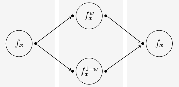
(a) Recovery of a possibility function by merging after splitting.

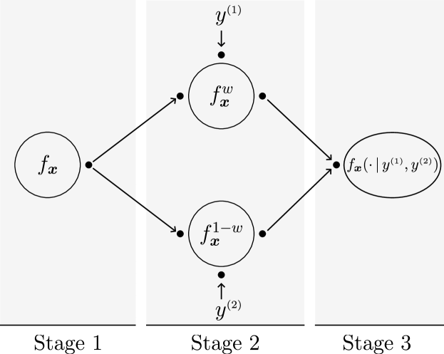
(b) Split-merge that involves conditionally-independent observations $y^{{\scriptscriptstyle(1)}}$ and $y^{{\scriptscriptstyle(2)}}$ yielding a posterior possibility function $f_{\bm{x}}(\cdot\,|\,y^{{\scriptscriptstyle(1)}},y^{{\scriptscriptstyle(2)}})$ based on the prior $f_{\bm{x}}$.

Figure 1: 3-stage process to split and merge the information in a possibility function, with and without additional observations.

These results already hint at the capabilities of possibility theory in terms of distributed inference: One can share information across a sensor network, update it with new observations and then recombine all this information in a natural way as depicted in Figure 1.

III Decentralised possibilistic Bayesian inference

In this section, we show how decentralised Bayesian inference can be asymptotically exact using possibility theory. We first focus on the case where observations are conditionally independent before showing how the principle of the existing geometric average fusion technique can be recovered in the case where there is a correlation between observations, with different levels of information regarding this correlation.

We consider a prior possibility function $f$ on a given set $S$ and model the evolution of the underlying state by a (possibilistic) Markov transition $g(\cdot\,|\,x)$, which is a possibility function on $S$ for any $x\in S$. In this context, if $n$ observations $y_{1},\dots,y_{n}$ are received and if these observations are described by a possibility function of the form $h(y_{1},\dots,y_{n}\,|\,x)=\prod_{i=1}^{n}h^{{\scriptscriptstyle(}i{\scriptscriptstyle)}}(y_{i}\,|\,x)$, for any $x\in S$, then the standard (non-distributed) approach is to consider the network’s posterior possibility function

$$f(x\,|\,y_{1},\dots,y_{n})\propto\bigg{[}\prod_{i=1}^{n}h^{(i)}(y_{i}\,|\,x)\bigg{]}\sup_{x^{\prime}\in S}g(x\,|\,x^{\prime})f(x^{\prime}).$$ (13)

This posterior possibility function is what we are trying to recover in the decentralised case.

We now consider $n$ sensors nodes $\mathrm{S}_{i}$ with $i\in\mathcal{V}=\{1,\dots,n\}$ and assume that the sensor network is modelled by an undirected connected graph $\mathcal{G}=(\mathcal{V},\mathcal{E})$ where $\mathcal{E}$ is the set of edges over which the nodes can communicate. Each node collects its independent observations of the same underlying variable. We refer to this configuration as decentralised fusion. We will use the superscript $\cdot^{(i)}$ to refer to quantities that are specific to sensor node $\mathrm{S}_{i}$. We denote by $\mathcal{N}_{i}=\{j\in\mathcal{V}:\{i,j\}\in\mathcal{E}\}$ the set of neighbours of $i\in\mathcal{V}$. We assume that the total number of nodes in the network is known by every node; this can indeed be obtained in a decentralised manner via standard techniques [30]. The objective in this section is to show that the posterior possibility function $f(\cdot\,|\,y_{1},\dots,y_{n})$ defined in (13) can be recovered by alternating between communicating on the network and fusing the received information at each node using (9).

One step of the decentralised algorithm is specified as follows: let us first follow the principles of Proposition 3 and share the prior information across the network after splitting into $f^{{\scriptscriptstyle(}i{\scriptscriptstyle)}}=f^{\omega_{i}}$ at node $i\in\mathcal{V}$ for some collection of non-negative weights $\{\omega_{i}\}_{i\in\mathcal{V}}$. Performing prediction at each node with the Markov transition $g$ would cause a large overlap between each local possibility function: if all nodes were to be connected to a central node $\mathrm{C}$ and fused, there would be no way of recovering the predicted possibility function $\sup_{x\in S}g(\cdot\,|\,x)f(x)$. Instead, we share the information about the evolution of the state by considering the Markov transition $g^{\varpi_{i}}(\cdot\,|\,x)$ at $\mathrm{S}_{i}$, for some collection of non-negative weights $\{\varpi_{i}\}_{i\in\mathcal{V}}$.

Finally, we assume that the observations are local, i.e. $y_{i}$ is the only observation at $\mathrm{S}_{i}$. As a result, the local posterior possibility function at node $i$ can be computed as

$$f^{(i)}(x\,|\,y_{i})\propto h^{(i)}(y_{i}\,|\,x)\sup_{x^{\prime}\in S}g^{\varpi_{i}}(x\,|\,x^{\prime})f^{\omega_{i}}(x^{\prime}).$$

The method we propose is reminiscent of iterative message-passing approaches to decentralised inference [1]: we assume that each node $j\in\mathcal{V}$ communicates with its neighbours and combines the information it receives by using a collection of non-negative weights $\{\Gamma_{i,j}\}_{{i,j}\in{\cal N}}$, where $\Gamma_{i,j}=0$ if $i\notin{\cal N}_{j}$, using

$$f^{(j,l)}(x)\propto {\Big{(}f^{(j,l-1)}(x)\Big{)}^{\Gamma_{j,j}}\mspace{-4.0mu}\prod_{i\in\mathcal{N}_{j}}\Big{(}f^{(i,l-1)}(x)\Big{)}^{\Gamma_{i,j}}},$$ (14)

$$= \prod_{i\in\mathcal{V}}\Big{(}f^{(i,l-1)}(x)\Big{)}^{\Gamma_{i,j}}\quad l=1,\dots,L$$

The initial condition of the iterations is selected as $f^{{\scriptscriptstyle(i,0)}}=f^{{\scriptscriptstyle(i)}}(\cdot\,|\,y_{i})$, so that the independence of the terms on the right hand-side of (14) are maintained for all steps $l=1,\dots,L$ following from the independence of the local posterior possibility functions $f^{{\scriptscriptstyle(i)}}(\cdot\,|\,y_{i})$ at $l=1$.

Let us denote by $\Gamma$ the weight matrix $(\Gamma_{i,j})_{i,j\in\mathcal{V}}$. The $l$th power of this matrix $\Gamma^{l}$ is related to the locally fused result in (14) by

$$f^{(j,l)}(x)= \prod_{i\in\mathcal{V}}\Big{(}f^{(i,0)}(x)\Big{)}^{\Gamma^{l}_{i,j}},$$

$$= \prod_{i\in\mathcal{V}}\Big{(}f^{(i)}(x\,|\,y_{i})\Big{)}^{\Gamma^{l}_{i,j}},\quad l=1,\dots,L,$$

so, we focus on the limiting case $\Gamma^{l}\xrightarrow{l\to\infty}\Gamma^{*}$. In turn, the $(i,j)$-th entry of $\Gamma^{*}$ is denoted by $\Gamma^{*}_{i,j}$, which we assume positive for any $i,j\in\mathcal{V}$. Therefore, the product of the locally fused possibility functions in the limit is given by

$$\hat{f}(x)\propto \prod_{j\in\mathcal{V}}\bigg{[}\prod_{i\in\mathcal{V}}\Big{(}f^{(i)}(x\,|\,y_{i})\Big{)}^{\Gamma^{*}_{i,j}}\bigg{]},$$

$$= \prod_{i,j\in\mathcal{V}}\Big{(}f^{(i)}(x\,|\,y_{i})\Big{)}^{\Gamma^{*}_{i,j}}.$$ (15)

Let us now investigate the conditions under which the result of the decentralised inference scheme in (14), (15) matches the network posterior in (13). We consider the following conditions

A1

It holds that $\omega_{i}=\varpi_{i}$ for all $i\in\mathcal{V}$ and that $\sum_{i\in\mathcal{V}}\omega_{i}=1$

A2

The limit condition for the weights in (14) as $l\rightarrow\infty$ is that $\Gamma^{*}_{i,j}=1/n$ for all $i,j\in\mathcal{V}$

The following theorem demonstrates that under these assumptions, the fused posterior $\hat{f}$ is equal to the posterior possibility function $f(\cdot\,|\,y_{1},\dots,y_{n})$.

Theorem 1.

Under Assumptions A1 and A2, the proposed decentralised Bayesian inference algorithm is (asymptotically) exact, i.e. the right hand-side of (15) equals to the network’s posterior possibility in (13).

Before its proof, a crucial aspect of Theorem 1 should be noted; it makes no assumptions on the nature of the set $S$ on which the fusion is performed. In particular, it does not rule out hierarchical problems such as the ones appearing in multi-target tracking, where both the number of targets and their respective state must be inferred. We illustrate this aspect in Section V where fusion is performed in a case where the existence of a target is uncertain; we then show in Section VI that Theorem 1 can be verified in practice for such problems despite the use of approximations.

Proof.

Let us express the fused result in the limit case given by (15) in a more explicit fashion as

$$\hat{f}(x) \propto\prod_{i,j\in\mathcal{V}}\Big{[}h^{(i)}(y_{i}\,|\,x)\sup_{x^{\prime}\in S}g^{\varpi_{i}}(x\,|\,x^{\prime})f^{\omega_{i}}(x^{\prime})\Big{]}^{\Gamma^{*}_{i,j}}$$

$$\mspace{-5.0mu}=\prod_{i,j\in\mathcal{V}}h^{(i)}(y_{i}\,|\,x)^{\Gamma^{*}_{i,j}}\sup_{x^{\prime}\in S}g^{\varpi_{i}\Gamma^{*}_{i,j}}(x\,|\,x^{\prime})\big{(}f(x^{\prime})\big{)}^{\omega_{i}\Gamma^{*}_{i,j}}.$$

For $\hat{f}=f(\cdot\,|\,y_{1},\dots,y_{n})$ to hold, a necessary (but not sufficient) condition is $\Gamma^{*}_{i,j}=1/n$; otherwise the contribution from the likelihood $h^{{\scriptscriptstyle(}i{\scriptscriptstyle)}}(y_{i}\,|\,\cdot)$ would not match the one in (13) in general (that is, except if $h^{{\scriptscriptstyle(}i{\scriptscriptstyle)}}(y_{i}\,|\,\cdot)$ takes value in $\{0,1\}$, in which case raising it to a positive finite power has no effect). It remains to match the contributions from the prediction step(s). We now have

$$\hat{f}(x)\propto\bigg{[}\prod_{i\in\mathcal{V}}h^{(i)}(y_{i}\,|\,x)\bigg{]}\bigg{[}\prod_{i\in\mathcal{V}}\sup_{x^{\prime}\in S}g^{\varpi_{i}}(x\,|\,x^{\prime})f^{\omega_{i}}(x^{\prime})\bigg{]}.$$

Sufficient conditions for $\hat{f}=f(\cdot\,|\,y_{1},\dots,y_{n})$ to hold are $\sum_{i\in\mathcal{V}}\omega_{i}=1$ and $\omega_{i}=\varpi_{i}$ for all $i\in\mathcal{V}$. Indeed, under these conditions, we have

$$\prod_{i\in\mathcal{V}}\sup_{x^{\prime}\in S}g^{\varpi_{i}}(x\,|\,x^{\prime})f^{\omega_{i}}(x^{\prime}) =\prod_{i\in\mathcal{V}}\Big{[}\sup_{x^{\prime}\in S}g(x\,|\,x^{\prime})f(x^{\prime})\Big{]}^{\omega_{i}}$$

$$=\sup_{x^{\prime}\in S}g(x\,|\,x^{\prime})f(x^{\prime}),$$

which concludes the proof of the theorem. ∎

Theorem 1 does not impose any constraints on the values of $\{\omega_{i}\}_{i\in\mathcal{V}}$ other than that they are in the $(n-1)$-dimensional simplex. The choice $\omega_{i}=1/n$ is particularly convenient as it leads to every node $i\in\mathcal{V}$ containing exactly $1/n$-th of the posterior information, i.e. it holds that

$$f^{(i,\infty)}(x)=f(x\,|\,y_{1},\dots,y_{n})^{1/n},\qquad i\in\mathcal{V}.$$

In other words, the locally fused possibility function at each node can be raised to the power $n$ to exactly find the network’s posterior; this scheme becomes an exact decentralised inference scheme.

We now consider an immediate corollary to Theorem 1 which considers the case where $\mathcal{G}$ is complete, i.e. there is an edge between every pair of nodes, with the following modified assumption:

A2’

It holds that $\mathcal{G}$ is complete and that $\Gamma_{i,j}=1/n$ for all $i,j\in\mathcal{V}$.

Corollary 2.

Under Assumptions A1 and A2’, the proposed decentralised Bayesian inference algorithm is exact.

To prove Corollary 2, it is sufficient to notice that under Assumption A2’, it holds that $\Gamma=\Gamma^{*}$, i.e., the asymptotic regime can be achieved in a single iteration.

Remark 2.

Let us consider the case where there is a central node $\mathrm{C}$ to which all the sensors are connected and which is the only node performing fusion. We refer to this scheme as centralised fusion. Since decentralised fusion with a complete graph is equivalent to centralised fusion, it holds that centralised fusion can also be performed exactly under Assumptions A1 and A2’.

Remark 3.

The results of Theorem 1 and Corollary 2 still hold if we replace the possibility function $h(y_{1},\dots,y_{n}\,|\,x)$ by a probability distribution of the form $p(y_{1},\dots,y_{n}\,|\,x)=\prod_{i=1}^{n}p^{{\scriptscriptstyle(}i{\scriptscriptstyle)}}(y_{i}\,|\,x)$. Indeed, the corresponding posterior, obtained through the form of Bayes theorem defined in (5), remains a possibility function and can therefore be discounted and/or fused similarly. In fact, the likelihood can also be a more complex object that involves both possibility functions and probability distributions with no effect on the result. An example of such a likelihood is provided in Section IV.

Remark 4.

In the linear-Gaussian case, one can use the possibilistic version of the Kalman filter [25] to perform Bayesian inference. The possibilistic Kalman filter has the same expected value and variance as the standard Kalman filter and, in the centralised case, the proposed approach reduces to the optimal fusion rule in the independent case [31].

IV The possibilistic Bernoulli filter

IV-A General recursion

In this section, we recall the equations of the possibilistic Bernoulli filter [12] and the underlying notion of Bernoulli uncertain finite set (UFS). The latter can be introduced as an uncertain variable $\bm{X}$ on the set $\mathsf{X}=\{\emptyset\}\cup\{\{x\}:x\in S\}$, which is the set of finite subsets of a given space $S\subseteq\mathbb{R}^{d}$ with no more than one element. The UFS $\bm{X}$ can be described by a possibility function $F$ on $\mathsf{X}$, and we will adopt the convention

$$F(X)=\begin{cases*}\beta&if $X=\emptyset$\\ \alpha f(x)&if $X=\{x\}$ with $x\in S$.\end{cases*}$$ (16)

The fact that $F$ is a possibility function implies that $\alpha$ and $\beta$ are non-negative, $\max\{\alpha,\beta\}=1$, and $f$ is a possibility function on $S$. The possibilistic Bernoulli filter is a recursion for a possibility function of the same form as $F$ describing the possibility of existence $\alpha$ of a target in $S$ and the information about its state via $f$. We follow the notations of Section III to describe a target’s dynamics and observation when it exists. We model the changes in cardinality by a transition matrix $(\tau_{ij})_{i,j\in\{0,1\}}$, where $\tau_{ij}$ corresponds to transitioning from cardinality $i\in\{0,1\}$ to cardinality $j\in\{0,1\}$. For instance, $\tau_{01}$ is the possibility of birth. The spatial information about birth is described by a possibility function $f_{\mathrm{b}}$ on $S$. Denoting by $F_{k-1}$ the Bernoulli possibility function describing the state and existence of the target at time $k-1$, given the observations up to time $k-1$, and following the convention of (16), we can now express $F_{k|k-1}$, the predicted Bernoulli possibility function at $k$, as

$$F_{k|k-1}(X)=\begin{cases*}\beta_{k|k-1}&if $X=\emptyset$\\ \alpha_{k|k-1}f_{k|k-1}(x)&if $X=\{x\}$ with $x\in S$.\end{cases*}$$ (17)

with

$$\beta_{k|k-1} =\max\{\beta_{k-1}\tau_{00},\alpha_{k-1}\tau_{10}\}$$ (18a)

$$\alpha_{k|k-1} =\max\{\beta_{k-1}\tau_{01},\alpha_{k-1}\tau_{11}\}$$ (18b)

$$f_{k|k-1}(x) =\alpha_{k|k-1}^{-1}\max\big{\{}\beta_{k-1}\tau_{01}f_{\mathrm{b}}(x),\alpha_{k-1}\tau_{11}\tilde{f}(x)\big{\}},$$ (18c)

where $\tilde{f}(x)=\sup_{x^{\prime}\in S}g(x\,|\,x^{\prime})f_{k-1}(x^{\prime})$ is the predicted possibility function describing the state of the target assuming that it exists at both times $k-1$ and $k$.

As opposed to the approach in [12], we consider a partially-probabilistic observation model where the detection and the data association are possibilistic and where the generation of false alarms and of the observation under the assumption of detection are probabilistic. We assume as is usual that at most one observation originates from the target. This yields a likelihood $\ell(Y_{k}\,|\,X)$ for the observation set $Y_{k}$ at time $k$ characterised by $\ell(Y_{k}\,|\,\emptyset)=\kappa(Y_{k})$ and

$$\ell(Y_{k}\,|\,\{x\})=\max\big{\{}\beta_{\mathrm{d}}\kappa(Y_{k}),\max_{y\in Y_{k}}\alpha_{\mathrm{d}}p(y\,|\,x)\kappa(Y_{k}\setminus\{y\})\big{\}},$$

where $\kappa$ is the density of the random finite set characterising the false alarms, where $\alpha_{\mathrm{d}}$ and $\beta_{\mathrm{d}}$ are respectively the possibilities of detection and non-detection, and where $p(\cdot\,|\,x)$ is the probability distribution of the observation given that the target is detected at state $x\in S$. The likelihood $\ell(\cdot\,|\,X)$ is neither a possibility function nor a probability distribution and its derivation requires more advanced notions which are relegated to the appendix.

Despite the considered partially-probabilistic approach, the form of the likelihood is similar to the one in [12] and the updated possibility function $F_{k}$ can be found in the same way: Following the same convention as before, we obtain

$$\beta_{k} \propto\ell(Y_{k}\,|\,\emptyset)\beta_{k|k-1}=\kappa(Y_{k})\beta_{k|k-1}$$ (19a)

$$\alpha_{k} \propto\alpha_{k|k-1}\sup_{x\in S}\ell(Y_{k}\,|\,\{x\})f_{k|k-1}(x)$$ (19b)

$$f_{k}(x) =\dfrac{\ell(Y_{k}\,|\,\{x\})f_{k|k-1}(x)}{\sup_{x\in S}\ell(Y_{k}\,|\,\{x\})f_{k|k-1}(x)},$$ (19c)

where $\max\{\alpha_{k},\beta_{k}\}=1$. Although it has limited influence on the form of the updated possibility function $F_{k}$, the introduction of the probabilistic elements $\kappa$ and $p(\cdot\,|\,x)$ allows for better connecting the proposed approach with the existing literature and hints at the potential for introducing more sophisticated mixed models in the future.

IV-B Implementation

For the sake of simplicity, we assume that the dynamics and likelihood are Gaussian, i.e. there exist matrices $G$, $Q$, $H$, $R$ of appropriate dimensions such that $g(x\,|\,x^{\prime})=\overline{\mathrm{N}}(x;Gx^{\prime},Q)$ and $p(y\,|\,x)=\mathrm{N}(y;Hx,R)$, with $Q$ and $R$ positive definite. The non-linear case has been considered in [12]. We also assume that the possibility function $f_{\mathrm{b}}$ is a max-mixture of Gaussian possibility functions of the form

$$f_{\mathrm{b}}(x)=\max_{i\in\{1,\dots,N_{\mathrm{b}}\}}w_{\mathrm{b},i}\overline{\mathrm{N}}(x;\mu_{\mathrm{b},i},P_{\mathrm{b},i}),$$

with $\{w_{\mathrm{b},i}\}_{i=1}^{N_{\mathrm{b}}}$ a collection of non-negative weights such that $\max_{i\in\{1,\dots,N_{\mathrm{b}}\}}w_{\mathrm{b},i}=1$, and with $\mu_{\mathrm{b},i}$ and $P_{\mathrm{b},i}$ the expected value and covariance matrix of the $i$-th term, respectively. These assumptions allow to write the recursion of the possibilistic Bernoulli filter in closed form as follows. If the possibility function $f_{k-1}$ is of the form

$$f_{k-1}(x)=\max_{i\in\{1,\dots,N_{\mathrm{k-1}}\}}w_{k-1,i}\overline{\mathrm{N}}(x;\mu_{k-1,i},P_{k-1,i}),$$

then the predicted possibility function $f_{k|k-1}$ follows as

$$f_{k|k-1}(x)=\alpha_{k|k-1}^{-1}\max\big{\{}\beta_{k-1}\tau_{01}f_{\mathrm{b}}(x),\alpha_{k-1}\tau_{11}$$

$$\quad\times\max_{i\in\{1,\dots,N_{\mathrm{k-1}}\}}w_{k-1,i}\overline{\mathrm{N}}(x;G\mu_{k-1,i},GP_{k-1,i}G^{\intercal}+Q)\big{\}},$$

which is also a max-mixture of Gaussian possibility functions which can be expressed using $N_{k|k-1}=N_{k-1}+N_{\mathrm{b}}$ Gaussian terms, the $i$-th one having weight $w_{k|k-1,i}$, expected value $\mu_{k|k-1,i}$ and covariance matrix $P_{k|k-1,i}$. The expressions of $\alpha_{k|k-1}$ and $\beta_{k|k-1}$ are unaffected by the form of $f_{k-1}$ are therefore not repeated. For the update step, the expression of $\alpha_{k}$ can be specialised to the Gaussian case as

$$\alpha_{k}\propto\alpha_{k|k-1}\max_{i\in\{1,\dots,N_{k|k-1}\}}w_{k|k-1,i}\max\big{\{}\beta_{\mathrm{d}}\kappa(Y_{k}),$$

$$\quad\max_{y\in Y_{k}}\alpha_{\mathrm{d}}\kappa(Y_{k}\setminus\{y\})\overline{\mathrm{N}}(x;H\mu_{k|k-1,i},HP_{k|k-1,i}H^{\intercal}+R)\big{\}},$$

The updated possibility function $f_{k}$ is characterised by

$$f_{k}(x)\propto\max_{i\in\{1,\dots,N_{k|k-1}\}}w_{k|k-1,i}\max\big{\{}\beta_{\mathrm{d}}\kappa(Y_{k}),\\ \max_{y\in Y_{k}}\alpha_{\mathrm{d}}\kappa(Y_{k}\setminus\{y\})\overline{\mathrm{N}}(x;\tilde{\mu}_{k,i},\tilde{P}_{k,i})\big{\}}$$

with $\tilde{\mu}_{k,i}$ and $\tilde{P}_{k,i}$ the standard updated expected value and covariance matrix of the Kalman filter corresponding to the $i$-th predicted term. Although $f_{k}$ is once again a Gaussian max-mixture, it is usually necessary to apply pruning and merging to it, as is standard, in order to control the number of terms. The latter is done using the Hellinger distance due to the fact that it is a more conservative notion of distance than the Mahalanobis distance. Terms that are sufficiently close are then merged following the standard procedure, with the only difference being that the final weight of the merged term is the maximum of the weights of the terms being merged [13].

V Sensor fusion

Algorithm 1 Decentralised fusion at the sensor node $\mathrm{S}_{i}$

Input: Sequence of observation sets $(Y_{k})_{k=1}^{K}$ at $\mathrm{S}_{i}$; Total number of time steps $K$; Discount factor $\omega_{i}\in[0,1]$; Weight matrix $\Gamma$; Number of network iterations $L$

1:$N\leftarrow 0$

2:$\hat{\alpha}\leftarrow 1$, $\hat{\beta}\leftarrow 1$

3:for all $k\in\{1,\dots,K\}$ do

4:     # Discounted prediction

5:     $\alpha\leftarrow\max\{\hat{\beta}\tau_{01}^{\omega_{i}},\hat{\alpha}\tau_{11}^{\omega_{i}}\}$

6:     $\beta\leftarrow\max\{\hat{\beta}\tau_{00}^{\omega_{i}},\hat{\alpha}\tau_{10}^{\omega_{i}}\}$

7:     for all $j\in\{1,\dots,N\}$ do

8:         $w_{j}\leftarrow\hat{\alpha}\tau_{11}w_{j}/\alpha$

9:         $\mu_{j}\leftarrow G\mu_{i}$

10:         $P_{j}\leftarrow GP_{i}G^{\intercal}+Q/\omega_{i}$

11:     end for

12:     for all $j\in\{1,\dots,N_{\mathrm{b}}\}$ do

13:         $w_{N+j}\leftarrow\hat{\beta}\tau_{01}w_{\mathrm{b},j}^{\omega_{i}}/\alpha$

14:         $\mu_{N+j}\leftarrow\mu_{\mathrm{b},j}$

15:         $P_{N+j}\leftarrow P_{\mathrm{b},j}/\omega_{i}$

16:     end for

17:     $N\leftarrow N+N_{\mathrm{b}}$

18:     # Update

19:     $F^{{\scriptscriptstyle(}i{\scriptscriptstyle)}}\leftarrow\mathrm{LocalUpdate}\big{(}Y_{k},\alpha,\beta,(w_{j},\mu_{j},P_{j})_{j=1}^{N}\big{)}$

20:     # Fusion

21:     for all $l\in\{1,\dots,L\}$ do

22:         Broadcast $F^{{\scriptscriptstyle(}i{\scriptscriptstyle)}}$

23:         Receive $\{F^{(i^{\prime})}:i^{\prime}\in\mathcal{N}_{i}\}$ from neighbours

24:         for all $i^{\prime}\in\mathcal{N}_{i}$ do

25:              $F^{{\scriptscriptstyle(}i{\scriptscriptstyle)}}\leftarrow\mathrm{Fusion}(F^{{\scriptscriptstyle(}i{\scriptscriptstyle)}},F^{(i^{\prime})},\Gamma_{i,i},\Gamma_{i,i^{\prime}})$

26:         end for

27:     end for

28:     # Unpack information after fusion

29:     $\big{(}\hat{\alpha},\hat{\beta},(w_{j},\mu_{j},P_{j})_{j=1}^{N}\big{)}\leftarrow F^{{\scriptscriptstyle(}i{\scriptscriptstyle)}}$

30:end for

This section follows the approach introduced in Section III for the fusion of the Gaussian max-mixture possibilistic Bernoulli filters detailed in Section IV. As before, we focus on decentralised fusion for a network of $n$ sensors with nodes $\mathrm{S}_{i}$, $i\in\mathcal{V}=\{1,\dots,n\}$, and with connectivity represented by a graph $(\mathcal{V},\mathcal{E})$. To make the proposed approach more concrete, we describe it via the pseudo-code in Algorithms 1-3. Algorithm 1 describes the general recursion with prediction, update and fusion being performed sequentially at each time step. We consider these three parts in turn and justify the computations in Algorithm 1.

Prediction

As shown in Section III, the Markov transition needs to be discounted to preserve the independence between sensor nodes. In the considered Gaussian max-mixture implementation of the possibilistic Bernoulli filter, the Markov transition $G(\cdot\,|\,X_{k-1})$ on $\mathsf{X}$ is characterised by

$$G(X_{k}\,|\,\emptyset)=\begin{cases*}\tau_{00}&if $X_{k}=\emptyset$\\ \tau_{01}f_{\mathrm{b}}(x_{k})&if $X_{k}=\{x_{k}\}$,\end{cases*}$$

and

$$G(X_{k}\,|\,\{x_{k-1}\})=\begin{cases*}\tau_{10}&if $X_{k}=\emptyset$\\ \tau_{11}g(x_{k}\,|\,x_{k-1})&if $X_{k}=\{x_{k}\}$.\end{cases*}$$

The discounted version $G(\cdot\,|\,X_{k-1})^{\omega}$ of this Markov transition is of the same form, with each term simply being brought to the power $\omega\in[0,1]$. This allows for (17) and (18) to be used directly with, e.g., $\tau_{11}^{\omega}$ and $g(x_{k}\,|\,x_{k-1})^{\omega}$ instead of $\tau_{11}$ and $g(x_{k}\,|\,x_{k-1})$. Lines 5-11 in Algorithm 1 follow directly from these calculations and from the fact that Gaussian possibility functions are closed under exponentiation. A related and important result that is unique to possibility theory is that Gaussian max-mixtures are closed under power, indeed, for any Gaussian max-mixture $f$, say,

$$f(x)=\max_{i\in\{1,\dots,N\}}w_{i}\overline{\mathrm{N}}(x;\mu_{i},P_{i}),$$

for some $N\in\mathbb{N}$, some non-negative weights $w_{i}$ such that $\max_{i\in\{1,\dots,N\}}w_{i}=1$, and some collection $\{(\mu_{i},P_{i})\}_{i=1}^{N}$ of expected values and covariance matrices. It holds that $f^{\omega}$ is also a Gaussian max-mixture for any $\omega\in[0,1]$. In particular, it holds that

$$f^{\omega}(x)=\max_{i\in\{1,\dots,N\}}w_{i}^{\omega}\overline{\mathrm{N}}(x;\mu_{i},P_{i}/\omega).$$

This result justifies the discounted birth model implemented in Lines 12-17 of Algorithm 1.

Update

The $\mathrm{LocalUpdate}()$ function, described in Algorithm 2, implements directly the approach of Section IV-B. Indeed, based on the assumed conditional independence of the observations between sensor nodes, there is no redundancy to be corrected and therefore no particular discount to be applied. Line 16 of Algorithm 2 (as well as Line 12 of Algorithm 3) is a renormalisation of the weights to ensure that they have a maximum equal to $1$. In both algorithms, this is followed by a call to a $\mathrm{Reduction}()$ function which is a Gaussian max-mixture reduction function, performing pruning and merging; the only difference with standard merging techniques is that the weight of a set of merged components is the maximum of the merged weights, as detailed in [13].

Fusion

After the local update in Line 19 of Algorithm 1, we have independent information at sensor node $\mathrm{S}_{i}$, under the form of a local posterior possibility function $F^{{\scriptscriptstyle(}i{\scriptscriptstyle)}}_{k}$, and aim to produce a fused possibility function $\hat{F}_{k}$. A direct application of (9) yields the parameters of $\hat{F}_{k}$ as

$$\hat{\beta}_{k} =C^{-1}\prod_{j\in\mathcal{N}_{i}}\beta^{(i)}_{k}$$ (20a)

$$\hat{\alpha}_{k} =C^{-1}\sup_{x\in S}\prod_{j\in\mathcal{N}_{i}}\alpha^{(j)}_{k}f^{(j)}_{k}(x)$$ (20b)

$$\hat{f}_{k}(x) \propto\prod_{j\in\mathcal{N}_{i}}f^{(j)}_{k}(x)$$ (20c)

where $C$ is such that $\max\{\hat{\alpha}_{k},\hat{\beta}_{k}\}=1$. The products in (20) are computed by multiplying two terms at a time in Lines 24-26 of Algorithm 1, with the specific calculations for the case of a Gaussian max-mixture being given in Algorithm 3. These steps are repeated $L$ times.

Algorithm 2 $\mathrm{LocalUpdate}(Y,\alpha,\beta,(w_{j},\mu_{j},P_{j})_{j=1}^{N})$

Input: Observation set $Y=\{y_{1},\dots,y_{M}\}$; Gaussian max-mixture Bernoulli possibility function under the form $\big{(}\alpha,\beta,(w_{j},\mu_{j},P_{j})_{j=1}^{N}\big{)}$

1:for all $j\in\{1,\dots,N\}$ do

2:     # Detection failure

3:     $\hat{w}_{j}\leftarrow\beta_{\mathrm{d}}\kappa(Y)w_{j}$

4:     $\hat{\mu}_{j}\leftarrow\mu_{j}$

5:     $\hat{P}_{j}\leftarrow P_{j}$

6:     for all $m\in\{1,\dots,M\}$ do

7:         # Detection of $j$th component by $m$th observation

8:         $j^{\prime}\leftarrow mN+j$

9:         $c_{m,j}\leftarrow|2\pi R|^{-1/2}\overline{\mathrm{N}}(y_{m};H\mu_{j},HP_{j}H^{\intercal}+R)$

10:         $\hat{w}_{j^{\prime}}\leftarrow c_{m,j}\alpha_{\mathrm{d}}\kappa(Y\setminus\{y_{m}\})w_{j}$

11:         $(\hat{\mu}_{j^{\prime}},\hat{P}_{j^{\prime}})\leftarrow\mathrm{KalmanUpdate}(\mu_{j},P_{j})$

12:     end for

13:end for

14:# Renormalise weights

15:$u\leftarrow\max_{j}\hat{w}_{j}$

16:$(\hat{w}_{j})_{j=1}^{(M+1)N}\leftarrow(\hat{w}_{j})_{j=1}^{(M+1)N}/u$

17:# Pruning and merging

18:$(\tilde{w}_{j},\tilde{\mu}_{j},\tilde{P}_{j})_{j=1}^{N}\leftarrow\mathrm{Reduction}\big{(}(\hat{w}_{j},\hat{\mu}_{j},\hat{P}_{j})_{j=1}^{(M+1)N}\big{)}$

19:# Update possibility of presence

20:$\tilde{\alpha}\leftarrow u\alpha/\max\{u\alpha,\kappa(Y)\beta\}$

21:$\tilde{\beta}\leftarrow\kappa(Y)\beta/\max\{u\alpha,\kappa(Y)\beta\}$

Output: $F=\big{(}\tilde{\alpha},\tilde{\beta},(\tilde{w}_{j},\tilde{\mu}_{j},\tilde{P}_{j})_{j=1}^{N}\big{)}$

Algorithm 3 $\mathrm{Fusion}(F,F^{\prime},\gamma,\gamma^{\prime})$

Input: Two Gaussian max-mixture Bernoulli possibility functions under the form $F=\big{(}\alpha,\beta,(w_{j},\mu_{j},P_{j})_{j=1}^{N}\big{)}$ and $F^{\prime}=\big{(}\alpha^{\prime},\beta^{\prime},(w^{\prime}_{j},\mu^{\prime}_{j},P^{\prime}_{j})_{j=1}^{N^{\prime}}\big{)}$; Discount weights $\gamma$ and $\gamma^{\prime}$

1:# Fuse terms of Gaussian max-mixture

2:for all $j\in\{1,\dots,N\}$ do

3:     for all $j^{\prime}\in\{1,\dots,N^{\prime}\}$ do

4:         $m\leftarrow(j-1)N^{\prime}+j^{\prime}$

5:         $\hat{w}_{m}\leftarrow(w_{j})^{\gamma}(w^{\prime}_{j^{\prime}})^{\gamma^{\prime}}\overline{\mathrm{N}}(\mu_{j};\mu^{\prime}_{j^{\prime}},P_{j}/\gamma+P^{\prime}_{j^{\prime}}/\gamma^{\prime})$

6:         $\hat{P}_{m}\leftarrow\big{(}\gamma(P_{j})^{-1}+\gamma^{\prime}(P^{\prime}_{j^{\prime}})^{-1}\big{)}^{-1}$

7:         $\hat{\mu}_{m}\leftarrow\hat{P}_{m}\big{(}\gamma(P_{j})^{-1}\mu_{j}+\gamma^{\prime}(P^{\prime}_{j^{\prime}})^{-1}\mu^{\prime}_{j^{\prime}}\big{)}$

8:     end for

9:end for

10:# Renormalise weights

11:$u\leftarrow\max_{j}\hat{w}_{j}$

12:$(\hat{w}_{j})_{j=1}^{NN^{\prime}}\leftarrow(\hat{w}_{j})_{j=1}^{NN^{\prime}}/u$

13:# Pruning and merging

14:$(\tilde{w}_{j},\tilde{\mu}_{j},\tilde{P}_{j})_{j=1}^{N}\leftarrow\mathrm{Reduction}\big{(}(\hat{w}_{j},\hat{\mu}_{j},\hat{P}_{j})_{j=1}^{NN^{\prime}}\big{)}$

15:# Fuse possibilities of (non-)existence

16:$\tilde{\alpha}\leftarrow u\alpha\alpha^{\prime}/\max\{u\alpha\alpha^{\prime},\beta\beta^{\prime}\}$

17:$\tilde{\beta}\leftarrow\beta\beta^{\prime}/\max\{u\alpha\alpha^{\prime},\beta\beta^{\prime}\}$

Output: $\tilde{F}=\big{(}\tilde{\alpha},\tilde{\beta},(\tilde{w}_{j},\tilde{\mu}_{j},\tilde{P}_{j})_{j=1}^{N}\big{)}$

Remark 5.

If $n$ is large and $w_{i}=1/n$ for all $i\in\mathcal{V}$ then $g_{k}^{w_{i}}$ might be extremely uninformative and make inference at each node more challenging, especially if there is a substantial number of false alarms. This can be addressed if the sensor FoVs are different, in which case the information in a given region does not have to be communicated to sensors that do not observe it. This extension is however kept for future work.

VI Simulations

We aim to show that the required approximations, i.e. pruning and merging of the Gaussian max-mixture, and a limited number of hops on the sensor network do not significantly lower the performance of the proposed method; recalling that, without these approximations and limitations, the proposed method would be asymptotically exact. The considered baselines are the decentralised fusion algorithms for the Bernoulli filter based on geometric average [21], arithmetic average [22] as well as the iterated (i.e. non-distributed) versions of both the probabilistic and possibilistic Bernoulli filters.

We consider simulations designed using the units of the international system, which allows for making these units implicit. Specifically, we consider $K=25$ time steps of duration $\Delta=1$, where targets evolve according to a nearly-constant velocity model in the 2-dimensional Euclidean plane, i.e. $X_{k}=GX_{k-1}+U_{k}$ with $U_{k}\sim\mathrm{N}(0,Q)$ independently for any $k$, where

$$G=I_{2}\otimes\begin{bmatrix}1&\Delta\\ 0&1\end{bmatrix}\quad\text{and}\quad Q=\sigma^{2}I_{2}\otimes\begin{bmatrix}\Delta^{4}/4&\Delta^{3}/2\\ \Delta^{3}/2&\Delta^{2}\end{bmatrix},$$

and, $\sigma=0.5$ is the standard deviation of the process noise. We assume that all the sensors have the same parameters and omit the superscript $\cdot^{(i)}$ whenever appropriate. Only the location of targets is observed by the sensors, that is $Y_{k}^{{\scriptscriptstyle(}i{\scriptscriptstyle)}}=H(X_{k}-x_{\mathrm{s}}^{{\scriptscriptstyle(}i{\scriptscriptstyle)}})+V_{k}^{{\scriptscriptstyle(}i{\scriptscriptstyle)}}$ with $V_{k}^{{\scriptscriptstyle(}i{\scriptscriptstyle)}}\sim\mathrm{N}(0,\sigma^{\prime 2}I_{2})$ independently for any $k$ and any $i$, where $\sigma^{\prime}=5$ is the standard deviation of the observational noise and where

$$H=\begin{bmatrix}1&0&0&0\\ 0&0&1&0\end{bmatrix}.$$

The state space is therefore defined as $S=\mathbb{R}^{4}$ and we assume the observation space to be of the form $S^{\prime}=[0,1000]\times[0,1000]$. We consider the case of $n=4$ sensors, distributed across the corners of the square boundary of $S^{\prime}$.

Any given sensor has an edge connecting it to the $2$ closest sensors, one on each side of it. The weight matrix $\Gamma$ is defined based on the Metropolis weights [32] as is usual in decentralised fusion. We denote by $p_{\mathrm{d}}(x)=0.7$ the probability of detection at state $x\in S$ and by $p_{\mathrm{s}}(x)=1-10^{-3}$ the probability of survival at $x$. We model the birth of the target as follows: there is a probability $1/K$ for the target is born at any given time step and, when it is born, its state is drawn from $\frac{1}{4}\sum_{i=1}^{4}\mathrm{N}(\mu_{\mathrm{b},i},\Sigma_{\mathrm{b}})$, where each of the means $\mu_{\mathrm{b},1},\dots,\mu_{\mathrm{b},4}$ is one of $[500\pm 200,0,500\pm 200,0]^{\intercal}$ and where $\Sigma_{\mathrm{b}}$ is the diagonal matrix with diagonal $[25^{2},5^{2},25^{2},5^{2}]$. Yet, in practice, the times of birth and death of the target are predetermined in order to facilitate the interpretation of the results: it is born at time $5$ and disappears at time $20$. The number of false alarms is Poisson distributed with parameter $\lambda_{\mathrm{fa}}=25$, with the corresponding observations being drawn uniformly at random within $S^{\prime}$. Both probabilistic and possibilistic approaches rely on pruning of the Gaussian mixture and max-mixture components with a threshold of $10^{-3}$. For the merging of components, it is based on the Hellinger distance with a threshold of $0.5$. The presence of the target is confirmed in probabilistic methods when the probability of existence is greater than a given threshold. Since arithmetic average and geometric average methods behave differently, the threshold for the former ($\tau_{\mathrm{aa}}=0.7$) is different than the threshold for the latter ($\tau_{\mathrm{ga}}=0.95$). The mechanisms that the proposed approach relies on are close to the ones of the geometric average fusion so that the same threshold $\tau_{\mathrm{ga}}$ is used; yet, instead of requiring the possibility of presence $\alpha$ to be greater than $\tau_{\mathrm{ga}}$, we check if the possibility of non-existence $\beta$ is smaller than $1-\tau_{\mathrm{ga}}$. This is a more stringent test which amounts to requiring that the corresponding minimum subjective probability of presence be no smaller than $\tau_{\mathrm{ga}}$.

An important aspect of the considered possibilistic approach is that it does not take the above data-generating mechanism directly as a model, and instead translates it into possibility functions. The Gaussian possibility function describing the dynamics is assumed to take the same expected value and covariance matrices as in the true model, and target-wise parameters are translated as follows: for any $x\in S$, denoting by $S_{\mathrm{obs}}=\{x\in S:Hx\in S^{\prime}\}$ the observed subset of the state space, we set $\alpha_{\mathrm{s}}(x)=1$, $\alpha_{\mathrm{d}}(x)=\bm{1}_{S_{\mathrm{obs}}}(x)$ and $\beta_{\mathrm{d}}(x)=1-p_{\mathrm{d}}\bm{1}_{S_{\mathrm{obs}}}(x)$, which correspond to the interpretation of possibility function as upper bounds for probabilities, as detailed in [13].

Figure 2 corresponds to the case where $L=2$ iterations are performed for decentralised fusion, allowing for the information of each sensor to reach all other sensor while still being far from the asymptotic case where $\Gamma^{L}$ is the constant matrix where each component is equal to $1/n$. Figure 2 shows that possibilistic fusion largely outperforms its probabilistic counterpart for $4$ considered performance criteria. In Figure 2(a), where the performance is assessed via the OSPA metric [33], it is already clear that the loss incurred by the proposed decentralised fusion algorithm is negligible when compared to the asymptotic regime. Figure 2(b) and 2(c) confirm that there are advantages both in terms of localisation and of cardinality estimation, although the localisation error of the geometric average fusion is similar to the one of the proposed method after $5$ to $10$ time steps. Even though Figure 2(b) shows that the possibilistic methods initialise slightly faster than the iterated probabilistic algorithm, we do not consider this difference as significant as it can be due to the choice of confirmation threshold. The same remark can be made about the difference in cardinality error between the arithmetic average and geometric average fusion in Figure 2(b).

One of the advantages of the proposed method is that the variance of the Gaussian term with highest weight is not overestimated, as opposed to arithmetic/geometric average methods. This is illustrated in Figure 2(d), which shows the entropy $\log\det(2\pi e\hat{P}_{k})$, with $\hat{P}_{k}$ the updated covariance matrix of the Gaussian term with highest weight at time $k$. Although the localisation error of the geometric average fusion is close to the proposed method, there remains a substantial error in the estimated variance, which can negatively affect downstream tasks.

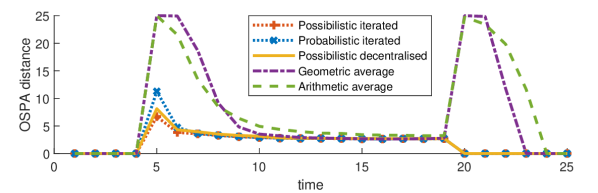
(a) OSPA distance with a cut off equal to $25$ and the Euclidian metric as basis for the localisation error

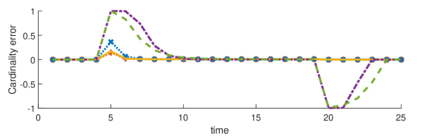
(b) Cardinality error: true cardinality minus estimated cardinality

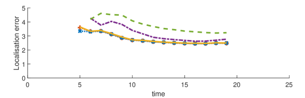
(c) Localisation error based on the Euclidean distance

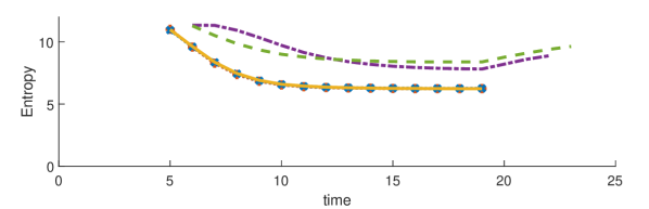
(d) Entropy of the Gaussian term with highest weight

Figure 2: Performance averaged over $1000$ Monte Carlo runs.

Finally, we study the behaviour of the proposed method with varying number of iterations. Table I gives the OSPA distance for $L=1$, $2$ and $4$ iterations, averaged over all $K=25$ time steps as well as over a $1000$ Monte Carlo runs. These results further validate the proposed method by showing a convergence to the asymptotic regime, even with a limited number of iterations. Given the structure of the sensor network, a single iteration is not sufficient for the information from each sensor to reach all other sensors, and the performance is more seriously affected in this case. For reference, the averaged OSPA distance for the geometric and arithmetic average fusion with $L=2$ iterations are both over $6$ due to the large cardinality error.

Table I: Averaged OSPA distance for possibilistic methods over all time steps and $1000$ Monte Carlo runs

Asymptotic (approximate)	Decentralised $L=4$	Decentralised $L=2$	Decentralised $L=1$
1.9045	1.9056	1.9458	2.3325

VII Conclusion

In this article, we have demonstrated how possibility theory allows for fusing and sharing information on a sensor network while preserving the optimality of non-distributed solutions. Maintaining the independence between sensor nodes was key in allowing decentralised fusion to fully leverage the observations of all sensors, leveraging unique properties of possibility theory. Despite the fact that the Bernoulli filter and its possibilistic counterpart perform similarly in single-sensor problems, significant gains were observed for decentralised networks. Future work includes improving the robustness to potential calibration errors of some of the sensors, hence leveraging the capabilities of possibility theory in terms of robust inference [34, 35].

-A Likelihood for the possibilistic Bernoulli filter

We first consider separately the probabilistic and possibilistic components of the likelihood. We model the uncertainty about the detection of the target as epistemic, with a possibility function characterised by $\alpha_{\mathrm{d}}$ for a detection and $\beta_{\mathrm{d}}$ for a detection failure. The uncertainty in the data association is considered epistemic as there is a true data association which is simply unknown. For the sake of simplicity, we re-express the observation set $Y$ as a vector $\tilde{y}=(y_{1},\dots,y_{m})$. Assuming that a detection has occurred, a possible association is defined as choosing a component of $\tilde{y}$ as the true detection, so that the other components are all false alarms. There is no prior information about the data association, which we model as permutations of indices in $\{1,\dots,m\}$, so we choose $\bm{1}$ as the corresponding possibility function.

If the target exists, is at state $x\in S$, and is detected, then the true observation $y$ is characterised by the conditional probability distribution $p(\cdot\,|\,x)$ and the false alarms are characterised by $\kappa$, with an underlying cardinality distribution $c$ on $\mathbb{N}$ and, assuming there are $n$ false alarms, with a p.d.f. $p_{n}$ on $(S^{\prime})^{n}$. In case of detection, the uncertainty in the observation is defined via an outer probability measure $\bar{P}_{\mathrm{d}}$ [10], characterised by

$$\bar{P}_{\mathrm{d}}(\varphi\,|\,x)=\sum_{n\geq 1}c(n-1)\int p(y^{\prime}_{1}\,|\,x)p_{n-1}(y^{\prime}_{2},\dots,y^{\prime}_{n})\times\\ \max_{\sigma}\big{(}\varphi(y^{\prime}_{\sigma(1)},\dots,y^{\prime}_{\sigma(n)})\big{)}\mathrm{d}y^{\prime}_{1}\dots\mathrm{d}y^{\prime}_{n}$$

for any real-valued function $\varphi$ taking vectors of observations as argument, where the maximum ranges over all permutations $\sigma$ of $\{1,\dots,n\}$. Setting $\varphi=\delta_{(y_{1},\dots,y_{m})}$ yields

$$\bar{P}_{\mathrm{d}}(y_{1},\dots,y_{m}\,|\,x)=c(m-1)\times\\ \max_{\sigma}p(y_{\sigma^{-1}(1)}\,|\,x)p_{m-1}(y_{\sigma^{-1}(2)},\dots,y_{\sigma^{-1}(m)}),$$

which can be simplified using the definition of $p_{n-1}$ as

$$\bar{P}_{\mathrm{d}}(y_{1},\dots,y_{m}\,|\,x)=\max_{y\in Y}p(y\,|\,x)\kappa(Y\setminus\{y\}).$$

Following the same steps, we find that the likelihood for the case where the target is not detecting is simply $\kappa(Y)$. Finally, taking the epistemic uncertainty regarding detection into account, we obtain the likelihood of interest.

References

- [1] M. Cetin, L. Chen, J. W. Fisher, A. T. Ihler, R. L. Moses, M. J. Wainwright, and A. S. Willsky, “Distributed fusion in sensor networks,” IEEE Signal Processing Magazine, vol. 23, no. 4, pp. 42–55, 2006.
- [2] S. Kar, S. Aldosari, and J. M. Moura, “Topology for distributed inference on graphs,” IEEE Transactions on Signal Processing, vol. 56, no. 6, pp. 2609–2613, 2008.
- [3] M. Uney and M. Cetin, “Monte Carlo optimization of decentralized estimation networks over directed acyclic graphs under communication constraints,” IEEE Trans. on Signal Proc., vol. 59, no. 11, pp. 5558–5576, 2011.
- [4] S. Kar and J. M. Moura, “Consensus + innovations distributed inference over networks: cooperation and sensing in networked systems,” IEEE Signal Processing Magazine, vol. 30, no. 3, pp. 99–109, 2013.
- [5] M. E. Liggins, C.-Y. Chong, I. Kadar, M. G. Alford, V. Vannicola, and S. Thomopoulos, “Distributed fusion architectures and algorithms for target tracking,” Proc. of the IEEE, vol. 85, no. 1, pp. 95–107, 1997.
- [6] D. Hall, C.-Y. Chong, J. Llinas, and M. Liggins II, Distributed data fusion for network-centric operations. Crc Press, 2017.
- [7] M. Üney, D. E. Clark, and S. J. Julier, “Distributed fusion of PHD filters via exponential mixture densities,” IEEE Journal of Selected Topics in Signal Processing, vol. 7, no. 3, pp. 521–531, 2013.
- [8] T. Li, X. Wang, Y. Liang, and Q. Pan, “On arithmetic average fusion and its application for distributed multi-Bernoulli multitarget tracking,” IEEE Transactions on Signal Processing, vol. 68, pp. 2883–2896, 2020.
- [9] J. Houssineau, N. Chada, and E. Delande, “Elements of asymptotic theory with outer probability measures,” arXiv preprint arXiv:1908.04331, 2019.
- [10] J. Houssineau, “Parameter estimation with a class of outer probability measures,” arXiv preprint arXiv:1801.00569, 2018.
- [11] D. Dubois and H. Prade, “Possibility theory and its applications: Where do we stand?,” in Springer Handbook of Computational Intelligence, pp. 31–60, Springer, 2015.
- [12] B. Ristic, J. Houssineau, and S. Arulampalam, “Target tracking in the framework of possibility theory: The possibilistic Bernoulli filter,” Information Fusion, vol. 62, pp. 81–88, 2020.
- [13] J. Houssineau, “A linear algorithm for multi-target tracking in the context of possibility theory,” IEEE Transactions on Signal Processing, vol. 69, pp. 2740–2751, 2021.
- [14] H. Cai, J. Houssineau, B. A. Jones, M. Jah, and J. Zhang, “Possibility generalized labeled multi-bernoulli filter for multi-target tracking under epistemic uncertainty,” IEEE Transactions on Aerospace and Electronic Systems (Early Access), 2022.
- [15] D. Dubois and H. Prade, “Possibility theory and data fusion in poorly informed environments,” Control Engineering Practice, vol. 2, no. 5, pp. 811–823, 1994.
- [16] D. Dubois, H. Prade, and R. Yager, “Merging fuzzy information,” in Fuzzy sets in approximate reasoning and information systems, pp. 335–401, Springer, 1999.
- [17] Y. Bar-Shalom, T. E. Fortmann, and P. G. Cable, “Tracking and data association,” Journal of the Acoustical Society of America, vol. 87, no. 2, pp. 918–919, 1990.
- [18] R. P. S. Mahler, Statistical Multisource-Multitarget Information Fusion. Artech House, 2007.
- [19] B. Ristic, B.-T. Vo, B.-N. Vo, and A. Farina, “A tutorial on Bernoulli filters: theory, implementation and applications,” IEEE Transactions on Signal Processing, vol. 61, no. 13, pp. 3406–3430, 2013.
- [20] S. P. Talebi and S. Werner, “Distributed Kalman filtering and control through embedded average consensus information fusion,” IEEE Transactions on Automatic Control, vol. 64, no. 10, pp. 4396–4403, 2019.
- [21] M. B. Guldogan, “Consensus Bernoulli filter for distributed detection and tracking using multi-static doppler shifts,” IEEE Signal Processing Letters, vol. 21, no. 6, pp. 672–676, 2014.
- [22] T. Li, Z. Liu, and Q. Pan, “Distributed Bernoulli filtering for target detection and tracking based on arithmetic average fusion,” IEEE Signal Processing Letters, vol. 26, no. 12, pp. 1812–1816, 2019.
- [23] B. De Baets, E. Tsiporkova, and R. Mesiar, “Conditioning in possibility theory with strict order norms,” Fuzzy Sets and Systems, vol. 106, no. 2, pp. 221–229, 1999.
- [24] D. Dubois, H. T. Nguyen, and H. Prade, “Possibility theory, probability and fuzzy sets misunderstandings, bridges and gaps,” in Fundamentals of fuzzy sets, pp. 343–438, Springer, 2000.
- [25] J. Houssineau and A. Bishop, “Smoothing and filtering with a class of outer measures,” SIAM/ASA Journal on Uncertainty Quantification, vol. 6, no. 2, pp. 845–866, 2018.
- [26] E. T. Jaynes, Probability theory: The logic of science. Cambridge university press, 2003.
- [27] S. J. Julier and J. K. Uhlmann, “A non-divergent estimation algorithm in the presence of unknown correlations,” in Proceedings of the 1997 American Control Conference, vol. 4, pp. 2369–2373, IEEE, 1997.
- [28] L. Chen, P. O. Arambel, and R. K. Mehra, “Estimation under unknown correlation: Covariance intersection revisited,” IEEE Transactions on Automatic Control, vol. 47, no. 11, pp. 1879–1882, 2002.
- [29] S. Destercke, D. Dubois, and E. Chojnacki, “Possibilistic information fusion using maximal coherent subsets,” IEEE Transactions on Fuzzy Systems, vol. 17, no. 1, pp. 79–92, 2008.
- [30] P. Jesus, C. Baquero, and P. S. Almeida, “A survey of distributed data aggregation algorithms,” IEEE Communications Surveys & Tutorials, vol. 17, no. 1, pp. 381–404, 2014.
- [31] K. H. Kim, “Development of track to track fusion algorithms,” in Proceedings of 1994 American Control Conference-ACC’94, vol. 1, pp. 1037–1041, IEEE, 1994.
- [32] G. C. Calafiore and F. Abrate, “Distributed linear estimation over sensor networks,” International Journal of Control, vol. 82, no. 5, pp. 868–882, 2009.
- [33] D. Schuhmacher, B.-T. Vo, and B.-N. Vo, “A consistent metric for performance evaluation of multi-object filters,” IEEE transactions on Signal Processing, vol. 56, no. 8, pp. 3447–3457, 2008.
- [34] B. Ristic, J. Houssineau, and S. Arulampalam, “Robust target motion analysis using the possibility particle filter,” IET Radar, Sonar & Navigation, vol. 13, no. 1, pp. 18–22, 2019.
- [35] J. Houssineau and D. J. Nott, “Robust bayesian inference in complex models with possibility theory,” arXiv preprint arXiv:2204.06911, 2022.