Mixing and diffusion in protoplanetary disc chemistry

We develop a simple iterative scheme to include vertical turbulent mixing and diffusion in ProDiMo thermo-chemical models for protoplanetary discs. The models are carefully checked for convergence toward the time-independent solution of the reaction-diffusion equations, as e.g. used in exoplanet atmosphere models. A series of five T Tauri disc models is presented where we vary the mixing parameter $\alpha_{\rm mix}$ from 0 to $10^{\,-2}$ and take into account (a) the radiative transfer feedback of the opacities of icy grains that are mixed upward and (b) the feedback of the changing molecular abundances on the gas temperature structure caused by exothermic reactions and increased line heating/cooling. We see considerable changes of the molecular and ice concentrations in the disc. The most abundant species (H2, CH4, CO, the neutral atoms in higher layers, and the ices in the midplane) are transported both up and down, and at the locations where these abundant chemicals finally decompose, for example by photo processes, the release of reaction products has important consequences for all other molecules. This generally creates a more active chemistry, with a richer mixture of ionised, atomic, molecular and ice species and new chemical pathways that are not relevant in the unmixed case. We discuss the impact on three spectral observations caused by mixing and find that (i) icy grains can reach the observable disc surface where they cause ice absorption and emission features at IR to far-IR wavelengths, (ii) mixing increases the concentrations of certain neutral molecules observable by mid-IR spectroscopy, in particular OH, HCN and C2H2, and (iii) mixing can change the optical appearance of CO in ALMA line images and channel maps, where strong mixing would cause the CO molecules to populate the distant midplane.

1 Introduction

Mixing and diffusion are important processes in chemical models for planetary atmospheres, see e.g. Moses et al. (2011); Hu et al. (2012); Parmentier et al. (2013); Kreidberg et al. (2014); Charnay et al. (2015); Rimmer & Helling (2016); Zhang & Showman (2018). In the deep layers of gas giant atmospheres, for instance, where densities and temperatures are high and the chemical reactions are fast, thermo-chemical equilibrium holds. With the falling temperatures and decreasing densities in higher layers, the chemical rates decrease and eventually become smaller than the turbulent eddy-mixing rates. Consequently, the molecular abundances become constant above a certain pressure level – an effect known as “transport-induced quenching” in planetary chemistry. Only at even higher altitudes, once the atmosphere becomes transparent to the stellar UV irradiation, the molecular abundances start to change again quickly due to photo-dissociation and photo-ionisation, beside other high-energy processes induced by cosmic rays, X-rays, and stellar energetic particles (SEPs), see e.g. Barth et al. (2021).

Another well-known effect in planetary chemistry is that above a certain layer called the homopause, the gas-kinetic micro-physical diffusion becomes more important than eddy-diffusion due to turbulent mixing (Hunten, 1973; Zahnle et al., 2016). This leads to molecule-dependent scale heights and changes of element abundances above the homopause which is essential to understand the transition into the exosphere.

In protoplanetary disc chemistry, despite the striking physical and chemical similarities to planetary atmospheres, mixing and diffusion have been rarely taken into account. The introduction of diffusive transport terms to the chemical rate equations requires a transition from first-order ordinary differential equations to second-order partial differential equations. Since disc chemistry is at least 2D, this means a considerable numerical and conceptual challenge.

Ilgner et al. (2004) pioneered the research on the impact of eddy mixing on disc chemistry in the frame of (1+1) D viscous disc evolution models for the innermost 10 au. They considered the sulphur molecules CS, SO, SO2, NS and HCS+ in particular, and concluded that vertical mixing is the most important process among all transport processes considered.

Semenov et al. (2006) used a similar approach but included gas-grain processes. They focused on the CO molecule in the outer disc regions. They concluded that CO can be considerably enhanced by vertical and radial mixing in the cold disc regions, where the dust temperature is lower than about 25 K and CO is expected to freeze out. The mixing rates were derived from an $\alpha$ disc model using $\alpha\!=\!10^{-2}$. They discussed the effects of radial, vertical, and “full 2D” mixing in a time-dependent disc model. Unfortunately, since this paper only has a single equation, it remains somewhat unclear how they actually solved the time-dependent partial differential equations.

Semenov & Wiebe (2011) studied the outer parts ($>$10 au) of DM Tau-like protoplanetary discs with given densities and temperatures. They distinguished between “responsive” and “unresponsive” molecules and ice species. Surprisingly, with regard to the results of this paper, CO, OH, H2O as well as water an ammonia ice were classified as “unresponsive”, i.e. their column densities were not altered much by the inclusion of mixing. In contrast, some sulphur-bearing molecules and poly-atomic (organic) molecules were found to be “hypersensitive”, i.e. their column densities were affected by more than 2 orders of magnitude. We note that these criteria are solely based on changes of the vertical column densities, which are not necessarily proportional to the observable line fluxes. In the T Tauri disc models presented in this paper, many of the prominent (sub-) mm lines are optically thick in the inner ($\mathrel{\mathchoice{\vbox{\offinterlineskip\halign{\hfil$\displaystyle#$\hfil\cr<\cr\sim\cr}}}{\vbox{\offinterlineskip\halign{\hfil$\textstyle#$\hfil\cr<\cr\sim\cr}}}{\vbox{\offinterlineskip\halign{\hfil$\scriptstyle#$\hfil\cr<\cr\sim\cr}}}{\vbox{\offinterlineskip\halign{\hfil$\scriptscriptstyle#$\hfil\cr<\cr\sim\cr}}}}$ 100 au) disc regions. In the mid-IR, the lines can also be covered by dust opacity. Hence the column densities, which are mostly set by the midplane concentrations, are no good predictors for line fluxes in many cases.

Heinzeller et al. (2011) used a simple numerical scheme to include advection caused by inward accretion and winds, and radial and vertical eddy-mixing in the thermo-chemical disc models developed by Nomura & Millar (2005). In their appendix, it becomes clear that an iterative approach was used, in which for each disc time integration step the adjacent concentrations were simply taken from the neighbouring cells at the previous time step and then assumed to be constant, while the central concentrations are advanced in time, point by point. We will follow this basic idea in this paper. We note, however, that their figure 1 seems to show some artefacts in the form of radial oscillations which could indicate that their numerical scheme is not fully converging. The results of Heinzeller et al. (2011) are complex, as many effects (vertical and radial mixing, winds, accretion) are discussed at the same time. They concluded that vertical mixing has a considerable impact on the disc chemistry and increases the abundances of many species in the warm molecular layer of the disc observable with the Spitzer Space Telescope and the James Webb Space Telescope (JWST). The viscous parameter for the turbulent mixing was set to $\alpha\!=\!10^{-2}$.

Common to the disc papers cited here is that the chemical mechanisms and pathways, which cause the observed changes in the models due to turbulent mixing, do not become fully clear. In this paper, we will concentrate on vertical mixing only, and will thoroughly explain and test our numerical approach. After an extended introduction to mixing and diffusion in Sect. 2, we explain our thermo-chemical disc model and test its convergence in Sect. 3. We systematically vary the $\alpha$-parameter that sets the strength of the turbulent mixing, and take the feedback of the changing concentrations on the gas temperature structure into account. We then show and discuss our results in Sect. 4, and demonstrate the main chemical mechanism that change the concentrations. We then continue in Sect. 5 to study the impact caused by turbulent mixing on a few observable quantities, such as ice emission and absorption features in the spectral energy distribution (SED), mid-IR molecular line emission features observable with JWST, and CO $J\!=\!2\to 1$ channel maps observable with Atacama Large Millimeter Array (ALMA). We conclude by summarising the main chemical mechanisms found and effects caused by turbulent mixing in protoplanetary discs in Sect. 6.

2 Chemistry with vertical mixing

2.1 Basic equations

The basic rate equation to solve for each chemical species is

$$\frac{\partial n_{i}}{\partial t}=P_{i}-L_{i}-\frac{\partial\Phi_{i}}{\partial z}\ ,$$ (1)

where $n_{i}\ \rm[cm^{-3}]$ is the particle density of species $i$, $P_{i}$ and $L_{i}$ $\rm[cm^{-3}s^{-1}]$ are the chemical production and destruction rates, and $\Phi_{i}\ \rm[cm^{-2}s^{-1}]$ is the diffusive particle flux according to Hu et al. (2012), Zahnle et al. (2016) and Rimmer & Helling (2016)

$$\Phi_{i}=-\,(K+D_{i})\,n\,\frac{\partial}{\partial z}\!\left(\frac{n_{i}}{n}\right)+D_{i}\,n_{i}\,\frac{(\mu-m_{i})\,g_{z}}{kT}\ ,$$ (2)

where $n\!=\!\sum_{i}n_{i}$ is the total particle density. $m_{i}$ is the mass of gas species $i$ and $\mu\!=\!\sum n_{i}m_{i}/n$ the mean molecular weight.$g_{z}\!=\!(GM_{\star}\,z)/(r^{2}+z^{2})^{3/2}\!=\!z\,\Omega^{2}$ is the gravitational acceleration in the vertical direction, $G$ the gravitational constant, $M_{\star}$ the mass of the central star, $r$ the distance from the rotation axis, $z$ the height over the midplane, and $\Omega$ is the Keplerian circular frequency. We have neglected here the “thermal diffusion factor” $\alpha_{T}$, which describes a second-order effect that the lightest molecules tend to diffuse towards the warmest places. The original derivation of Eq. (2) can be found in Hunten (1973) with further reading in Kuramoto et al. (2013).

$K\ \rm[cm^{2}/s]$ is the eddy-diffusion coefficient caused by turbulent mixing motions in the $z$-direction, sometimes also denoted by $k_{zz}$. $K$ is generally given by a characteristic mixing velocity times a characteristic length

$$K=\langle v_{z}\rangle\,L\ ,$$ (3)

where $L$ is the size of the largest eddy (“mixing length”) and $\langle v_{z}\rangle$ is the root-mean square of the fluctuating part of the vertical gas velocities. According to the $\alpha$-disc model of Shakura & Syunyaev (1973), the typical vertical length scale is given by the pressure scale height $L\approx H$ and the turbulent mixing velocity is approximated as $\langle v_{z}\rangle\approx\alpha_{\rm mix}\,c_{\rm s}$,

$$K=\alpha_{\rm mix}\,c_{\rm s}\,H\ ,$$ (4)

where $c_{\rm s}\!=\!\sqrt{kT/\mu}$ is the local isothermal sound speed and $T$ the temperature. Typical values used in the literature are $\alpha\!\approx\!10^{-5}\,...\,10^{-2}$ using different constraints, see reviews by Lesur et al. (2022) and Pinte et al. (2022). While theoretical accretion models often favour higher values to explain the mass accretion rates, see e.g. Manara et al. (2016); Mulders et al. (2017), observational contraints about turbulent line broadening (Flaherty et al., 2015) and dust settling (Pinte et al., 2018) suggest lower values. Eddy mixing transports all molecules in the same way. In contrast, the gas-kinetic micro-physical diffusion coefficient $D_{i}\ \rm[cm^{2}s^{-1}]$, due to Brownian motions,

$$D_{i}=\frac{1}{3}\frac{v_{{\rm th},i}}{\sigma_{\!ia}\,n}$$ (5)

depends on species $i$ because the collisional cross section $\sigma_{ia}$ depends on the “size” of the molecule $i$ and the relative velocity depends on its reduced mass $1/m_{\rm red}\!=\!1/m_{i}+1/m_{j}$. A simple hard-sphere approximation would be (Jeans, 1967)

$$D_{i} \!\!\!=\!\!\! \frac{1}{3}\left(\sum_{j}\frac{n_{j}\,\pi(r_{i}+r_{j})^{2}}{\sqrt{\frac{8\,kT}{\pi\,m_{\rm red}}}}\right)^{-1}$$ (6)

$$\!\!\!=\!\!\! \frac{1}{3}\sqrt{\frac{8\,kT}{\pi\,m_{i}}}\left(\sum_{j}\frac{n_{j}\,\pi(r_{i}+r_{j})^{2}}{\sqrt{1+\frac{m_{i}}{m_{j}}}}\right)^{-1}=\leavevmode\nobreak\ \frac{b_{ia}}{n}\ ,$$

where the effective radii of the molecules $r_{i}$ can be measured from viscosity experiments (Jeans, 1967), or calculated from Lennard-Jones potentials. $b_{ia}$ is called the binary diffusion coefficient $\rm[cm^{-1}s^{-1}]$ for collisions between species $i$ and a “background atmosphere” denoted by $a$. Some binary diffusion coefficients for a few relevant combinations of H, H₂ and CO₂ are given in Hu et al. (2012). Most atoms and molecules have effective collisional radii $r_{i}$ between about 1 Å and 3 Å, see Table 1. However, when the diffusion of charged particles and/or diffusion in plasma is considered, the Coulomb cross sections (Langevin cross-section) are larger, by orders of magnitude, than the geometrical cross sections, see e.g. section 2.5.2 in Wiesemann (2014).

Table 1: Effective molecular radii for diffusion coefficients calculated with the tools provided at Wolfram’s webpage${}^{\ref{foot1}}$ at $T\!=\!300\,$K

particle $i$	radius $r_{i}$
He	1.084 Å
H2	1.366 Å
O2	1.811 Å
CO	1.886 Å
N2	1.901 Å
CH4	2.075 Å
H2O	2.178 Å
CO2	2.304 Å

2.2 Location of the homopause

Equations (4) and (5) show that while the eddy-diffusion coefficient $K$ is assumed to be constant as function of height $z$, the molecular diffusion coefficient $D_{i}$ scales with $1/n$, i.e. it increases with height. In fact, in most parts of the disc, we have $K\!\!\gg\!\!D_{i}$. However, in the region above the $K\!\!=\!\!D_{i}$ layer, called the homopause (see Fig. 1), the molecules, atoms and ions will tend to arrange themselves with individual scale-heights, which could be denoted by “gravitational de-mixing”. Above the homopause, the concentrations of the heavy molecules drops quickly, whereas the lighter molecules keep on extending further up. This behaviour can be verified by considering the case of a non-reactive ($P_{i}\!=\!L_{i}\!=\!0$) mixture of ideal gases at constant temperature without eddy mixing ($K\to 0$) in equilibrium, where both $n(z)$ and $n_{i}(z)$ become time-independent functions of $z$. The diffusive fluxes vanish and we have

$$\Phi_{i}=0\leavevmode\nobreak\ =\leavevmode\nobreak\ -D_{i}\,n\,\frac{d}{dz}\!\left(\frac{n_{i}}{n}\right)+D_{i}\,n_{i}\,\frac{(\mu-m_{i})\,g_{z}}{kT}$$

$$\Rightarrow \frac{d}{dz}\ln\frac{n_{i}}{n}\leavevmode\nobreak\ =\leavevmode\nobreak\ \frac{(\mu-m_{i})\,g_{z}}{kT}\leavevmode\nobreak\ =\leavevmode\nobreak\ \frac{1}{H}-\frac{1}{H_{i}}$$

$$\Rightarrow n_{i}(z)=n_{i}(0)\exp\Big{(}-\frac{z}{H_{i}}\Big{)}\quad\mbox{and}\quad n(z)=n(0)\exp\Big{(}-\frac{z}{H}\Big{)}$$

with molecular and atmospheric scale heights $H_{i}=kT/(m_{i}g_{z})$ and $H=kT/(\mu g_{z})$, respectively.

Figure 1 shows the location of the homopause based on the ProDiMo model described in Sect. 3 for a couple of $\alpha_{\rm mix}$ values. A demonstration molecule with mass $m_{i}\!=\!20$ amu and radius $r_{i}\!=\!2\,$Å is considered, in a mixture of H+, H, H₂, He+ and He, with radii 0.8Å, 0.8Å, 1.366Å, 1.084Å and 1.084Å, respectively. The surprising conclusion from Fig. 1 is that gravitational de-mixing seems likely to play a significant role in the upper disc layers from which e.g. disc winds are launched, which can therefore be expected to contain only little amounts of heavy elements. We have neglected plasma effects here, i.e. increased Coulomb collisional cross sections, where the homopause would be located higher in the disc.

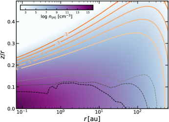
Figure 1: Location of the homopause, where the diffusion coefficients caused by eddy mixing and gas-kinetic motions are equal ($K\!=\!D_{i}$). The colours show the hydrogen nuclei density, $n_{\langle\rm H\rangle}$, as function of radius $r$ and relative height $z/r$. The coloured contour lines show where the homopause is situated when $K$ is calculated with different values of $\log_{\rm 10}\alpha_{\rm mix}$. The dashed lines show where the vertical optical extinction $A_{\rm V,ver}$ equals 100 (black), 10 (dark grey) and 1 (light grey). The dust opacities correspond to our un-mixed model described in Sect. 3. The uneven $A_{\rm V}$ contours are caused by the uneven spatial distribution of the ices, which are taken into account when calculating the opacities.

2.3 Can mixing change the element abundances?

An important question is whether the element abundances can be affected by diffusive transport and hence become spatially dependent quantities. The element abundances are given by

$$n_{\langle\rm H\rangle}\,\epsilon_{k}=\sum_{i}s_{i,k}n_{i}$$ (7)

where $s_{i,k}$ is the stoichiometric factor of element $k$ in molecule $i$, $\epsilon_{k}$ are the element abundances with respect to hydrogen, and $n_{\langle\rm H\rangle}$ is the total hydrogen nuclei particle density. $\epsilon_{\rm H}\!=\!1$ by definition. The changes of the element abundances follow from Eq. (1) after multiplication with $s_{i,k}$ for a selected element $k$ and summation over all chemical species $i$

$$\frac{\partial}{\partial t}\big{(}n_{\langle\rm H\rangle}\,\epsilon_{k}\big{)}=\sum_{i}s_{i,k}\Big{(}P_{i}-L_{i}\Big{)}-\sum_{i}\frac{\partial}{\partial z}\Big{(}s_{i,k}\Phi_{i}\Big{)}\ .$$ (8)

Chemical reactions conserve the element abundances, hence the first term in Eq. (8) vanishes. Concerning the diffusive flux $\Phi_{i}\rm\ [cm^{-2}s^{-1}]$ let us first consider the case $K\!\gg\!D_{i}$ where turbulent mixing dominates. From Eq. (2) we then have

$$\Phi_{i}=-K\,n\,\frac{\partial}{\partial z}\!\left(\frac{n_{i}}{n}\right)\ .$$ (9)

The diffusive element fluxes are hence given by

$$\Phi_{k} \!=\! \sum_{i}s_{i,k}\,\Phi_{i}\leavevmode\nobreak\ =\leavevmode\nobreak\ -\sum_{i}s_{i,k}\,K\,n\,\frac{\partial}{\partial z}\!\left(\frac{n_{i}}{n}\right)$$ (10)

$$\!=\! -K\,n\,\frac{\partial}{\partial z}\!\left(\frac{\sum_{i}s_{i,k}\,n_{i}}{n}\right)\leavevmode\nobreak\ =\leavevmode\nobreak\ -K\,n\,\frac{\partial}{\partial z}\!\left(\frac{n_{\langle\rm H\rangle}\,\epsilon_{k}}{n}\right)\ ,$$ (11)

where we have used that $K$ does not depend on molecule. If we can further assume that $n_{\langle\rm H\rangle}\!\propto\!n$ we find

$$\frac{\partial}{\partial t}\big{(}n_{\langle\rm H\rangle}\,\epsilon_{k}\big{)}\leavevmode\nobreak\ =\leavevmode\nobreak\ -\frac{\partial}{\partial z}\Phi_{k}\leavevmode\nobreak\ =\leavevmode\nobreak\ \frac{\partial}{\partial z}\bigg{(}K\,n_{\langle\rm H\rangle}\,\frac{\partial\epsilon_{k}}{\partial z}\bigg{)}\ .$$ (12)

Equation (12) states that eddy diffusion works against spatial gradients of element abundances. No matter how complicated the chemical processes are, eddy diffusion will always diminish such gradients $(\Phi_{k}\!\to\!0\leavevmode\nobreak\ \Rightarrow\leavevmode\nobreak\ \frac{\partial\epsilon_{k}}{\partial z}\!\to\!0$), making sure that the element abundances will eventually become constant throughout the disc.

This result seems a bit counter-intuitive at first, for example when we consider a particular molecule only, which is, for example, abundant in deep layers and mixed up where it dissociates, one would expect this process to enrich the higher layers with the elements the molecule was composed of. However, this is not how eddy mixing works. Mixing rather exchanges molecules for other molecules in the local neighbourhood, and if we properly sum up the total effect on the element abundances, via $\Phi_{k}=\sum_{i}s_{i,k}\,\Phi_{i}$, the net effect is exactly zero, unless there is a spatial gradient in element abundances in the first place, in which case eddy diffusion will reduce that gradient.

However, this conclusions is only valid as long as $K$ is independent of molecules/particle to be mixed by diffusion. Once we add $D_{i}$ with $D_{i}\!\mathrel{\mathchoice{\vbox{\offinterlineskip\halign{\hfil$\displaystyle#$\hfil\cr>\cr\sim\cr}}}{\vbox{\offinterlineskip\halign{\hfil$\textstyle#$\hfil\cr>\cr\sim\cr}}}{\vbox{\offinterlineskip\halign{\hfil$\scriptstyle#$\hfil\cr>\cr\sim\cr}}}{\vbox{\offinterlineskip\halign{\hfil$\scriptscriptstyle#$\hfil\cr>\cr\sim\cr}}}}\!K$ (above the homopause), we can no longer pull out the net diffusion coefficient $(K+D_{i})$ from the sum in Eq. (10). In that case, diffusion will change the element abundances. An example for such long-term effects by gravitational de-mixing was already described in Sect. 2.2.

Another relevant case occurs when we consider the difference between gaseous and ice species. The ice species are transported with the dust grains, and the grains are only moved by the larger turbulent eddies. In order to arrive at an effective dust particle diffusion coefficient, the advective effect of all individual turbulent eddies has to be averaged. This procedure has been carried out, with different methods and approximations, by Dubrulle et al. (1995), Schräpler & Henning (2004) and Youdin & Lithwick (2007). The result of Schräpler & Henning (2004, see their Eq. 27), is

$$K_{\rm ice}=\frac{K}{1+{St}}$$ (13)

where ${St}$ is the Stokes number given by

$${St}=\frac{\tau_{\rm stop}}{\tau_{\rm eddy}}=\frac{\frac{\rho_{\rm d}\,a}{\rho\,v_{\rm th}}}{\frac{H}{\alpha_{\rm mix}\,c_{\rm s}}}=\sqrt{\frac{\pi}{8}}\,\frac{\rho_{\rm d}\,a\,\alpha_{\rm mix}}{\rho\,\,H}$$ (14)

where $\tau_{\rm stop}$ is the stopping distance, $\tau_{\rm eddy}$ the turnover timescale of the largest turbulent eddy, $\rho_{\rm d}$ the dust material density, $v_{\rm th}$ the thermal velocity, $c_{\rm s}$ the sound velocity, $H$ the pressure scale height and $a$ is the grain radius. The factor $\sqrt{\pi/8}$ is because $c_{\rm s}^{2}=kT/\mu$ but $v_{\rm th}^{2}=8kT/(\pi\mu)$.

It is questionable, however, in how far Eq. (13) describes the actual dynamical motions of dust grains with large Stokes numbers in disks. The main reason is that such particles will start to migrate inward, i.e. they develop a systematic velocity with respect to the gas, which goes beyond the mixing approach. Such motions have been shown to be able to change the elemental abundances accross ice lines of key volatiles such as CO (Krijt et al., 2018). Furthermore, it is not obvious how to choose $a$ as we actually need the cumulative effect of all grains of different sizes on the diffusive flux, where it also must be debated how the ice is distributed onto the bare grains as function of size, and how the size dust distribution is altered by ice formation, see e.g. Arabhavi et al. (2022).

Assuming that we can determine $K_{\rm ice}$ anyway, and assuming that all vertical element fluxes $\Phi_{k}$ must vanish everywhere in the disc in the time-independent limiting case, we can derive a local condition for each element $k$ from Eq. (10):

$$\Phi_{k}=-K\,n\,\frac{\partial}{\partial z}\left(\frac{\sum_{\rm gas}s_{ik}n_{i}}{n}\right)-K_{\rm ice}\,n\,\frac{\partial}{\partial z}\left(\frac{\sum_{\rm ice}s_{ik}n_{i}}{n}\right)\leavevmode\nobreak\ =\leavevmode\nobreak\ 0\ .$$ (15)

Defining the element abundances present in the gas and ice, respectively, as

$$\epsilon_{k}=\epsilon_{k}^{\rm gas}\!+\!\epsilon_{k}^{\rm ice}\;\;,\;\;n_{\langle\rm H\rangle}\,\epsilon_{k}^{\rm gas}\!=\!\sum\limits_{i,\rm gas}s_{ik}n_{i}\;\;,\;\;n_{\langle\rm H\rangle}\,\epsilon_{k}^{\rm ice}\!=\!\sum\limits_{i,\rm ice}s_{ik}n_{i}$$ (16)

we find the following result that is independent of $\alpha_{\rm mix}$

$$\frac{\partial}{\partial z}\left(\frac{n_{\langle\rm H\rangle}\,\epsilon_{k}^{\rm gas}}{n}\right)+\frac{K_{\rm ice}}{K}\,\frac{\partial}{\partial z}\left(\frac{n_{\langle\rm H\rangle}\,\epsilon_{k}^{\rm ice}}{n}\right)\leavevmode\nobreak\ =\leavevmode\nobreak\ 0\ .$$ (17)

2.3.1 Small Stokes numbers

In the limiting case of small dust radii $a$ and/or large gas densities $\rho$, we have ${St}\ll 1$, i.e. well-coupled grains, and hence $K_{\rm ice}\approx K$. Thus, from Eq. (17), we obtain

$$\frac{n_{\langle\rm H\rangle}\,\epsilon_{k}}{n}=\ce{const}\ .$$ (18)

previously referred to as the case of “constant element abundances”. Clearly, when all species are transported in equal ways, and hence mixed with the same efficiency, the element abundances cannot change. However, Eq. (18) actually states a somewhat different result. Diffusion will make sure that, on the long run, the concentrations of elements as measured with respect to the total gas particle density $n$ become constant. At the locations of the major phase transitions $\ce{H+}\!\leftrightarrow\!\ce{H}$ and $\ce{H}\!\leftrightarrow\!\ce{H2}$, where the mean molecular weight changes by roughly a factor of 2 each, the element abundances must change as well, in the opposite direction, approximately $\epsilon_{k}\!\propto\!1/\mu$. Otherwise, when $\mu$ is constant, we have $n\propto n_{\langle\rm H\rangle}$ and hence indeed $\epsilon_{k}=\ce{const}$. Considering a complete vertical column, from ionised down to molecular conditions, Eq. (18) states that the helium abundance, for instance, should be about $4\times$ larger in the ionised regions as compared to the molecular regions.

2.3.2 Large Stokes numbers

In the limiting case of large Stokes numbers ($a\to\infty$ and/or $\rho\to 0$) we have $K_{\rm ice}\ll K$, and thus from Eq. (17)

$$\frac{n_{\langle\rm H\rangle}\,\epsilon_{k}^{\rm gas}}{n}=\ce{const}\ .$$ (19)

Equation (19) states a remarkable result. If an element can freeze out anywhere in the column, a rather low level of $\epsilon_{k}^{\rm gas}$ will be enforced there, and this low level of $\epsilon_{k}^{\rm gas}$ must be identical everywhere in the column to make the diffusive fluxes vanish, irrespective of the local $\epsilon_{k}^{\rm ice}$. This effect is commonly know as “cold trap”, see e.g. Krijt et al. (2016) and Öberg & Bergin (2021). Since a cold surface cannot move, but air does, the gaseous water molecules in a room will continue to diffuse toward and condense onto that cold surface, until eventually the supersaturation of the air over the cold surface approaches unity. If the surface temperature is kept lower than air temperature, this will eventually cause an under-saturation of water vapour in the warm gas in the room.

In a protoplanetary disc, we have the same principle situation. Certain molecules will freeze out quickly in the cold midplane, establishing very low local $\epsilon_{k}^{\rm gas}$. After just a few vertical mixing timescales (see Eq. 31), we would hence expect that most molecules in the upper layers should simply be mixed down into the midplane and freeze out there, leaving behind very low concentrations also in the upper layers.

But this conclusion would be in obvious conflict with ALMA observations, for example (Pinte et al., 2018; Rab et al., 2020), where we clearly see CO molecules only above the icy midplane at 100 au distances. We conclude that the cold trap effect cannot work in discs at full effect, possibly because:

• The actual $\alpha_{\rm mix}$ in discs is much lower than $10^{-2}$, such that the mixing timescale according to Eq. (31) approaches the disc lifetime. For an assumed disc lifetime of $5\times 10^{6}\,$yrs, this would suggest $\alpha_{\rm mix}<3\times 10^{-5}$ at 100 au, and even smaller $\alpha_{\rm mix}$ at smaller radii.

• The effective Stokes numbers (after averaging over dust size distribution) result to be small in Eq. (13), such that the limiting case described by Eq. (19) is not reached.

• A combination of both.

Even if these factors result in large deviations from Eq. (19), the cold trap effect could still cause important effects with respect to the case of constant element abundances (Eq. 18) over long timescales, which however will be difficult to prove observationally. In principle, one can solve Eq. (17) numerically, in an iterative way, to make it consistent with the ice chemistry, to obtain $\epsilon_{k}^{\rm gas}(z)$ and $\epsilon_{k}^{\rm ice}(z)$.

Further investigations are clearly required here, both about the influence of molecular diffusion on the upper disc layers and about the cold trap effect, where Eq. (17) could serve as a useful starting point. However, in the remaining parts of this paper, we will not discuss these complications any further, but concentrate on the most basic case, where we have vanishing molecular mixing $D_{i}\!\to\!0$ and no difference between the diffusive transport of gas and dust $K_{\rm ice}\!\to\!K$, in which case the element abundances can be assumed to be constant throughout in the disc. We also neglect here vertical gradients of the mean molecular weight $\mu$.

2.4 Implementation of mixing rates in ProDiMo

A direct numerical solution of the reaction-diffusion equations (Eq. 1), which is a system of coupled stiff partial differential equations of second order, is difficult and can be computationally very demanding, see Semenov et al. (2006); Semenov & Wiebe (2011) and Hu et al. (2012). Here, we follow an iterative approach similar to Heinzeller et al. (2011) and Rimmer & Helling (2016). We consider height grid points $\{z_{k}\,|\,k=1,...,K\}$. As shown in Appendix A, the divergence of the diffusive particle flux $i$ at point $k$ can be numerically discretised as

$$-\frac{\partial\Phi_{i,k}}{\partial z}={\cal A}\,n_{i,k+1}\leavevmode\nobreak\ -\leavevmode\nobreak\ {\cal B}\,n_{i,k}\leavevmode\nobreak\ +\leavevmode\nobreak\ {\cal C}\,n_{i,k-1}$$ (20)

where $n_{i,k}$ is the particle density of species $i$ at height grid point $k$, and where the coefficients ${\cal A}$, ${\cal B}$, ${\cal C}$ are given by the geometry of the grid points, the eddy and molecular diffusion coefficients, $K$ and $D_{i}$, and the total particle densities $n=\sum n_{i}$ at the neighbouring height grid points $k\!-\!1$, $k$, $k\!+\!1$. Our approach is then very simple. We consider the neighbouring concentrations $n_{i,k+1}$ and $n_{i,k-1}$ as fixed during the solution of the chemistry at height point $k$. Hence, we can solve

$$\frac{\partial n_{i}}{\partial t}=\tilde{P_{i}}-\tilde{L_{i}}\ ,$$ (21)

with the existing time-independent chemistry solver in the ProDiMo model, where

$$\tilde{P_{i}} = P_{i}+{\cal A}\,n_{i,k+1}+{\cal C}\,n_{i,k-1}$$ (22)

$$\tilde{L_{i}} = L_{i}+{\cal B}\,n_{i,k}\ .$$ (23)

Since ProDiMo solves the chemistry and heating/cooling balance on all grid points in a particular order (first downward – then outward, following the two main irradiation directions), the constant $n_{i,k+1}$ are taken from the same chemistry iteration (from the last point above just solved), whereas the constant $n_{i,k-1}$ are taken from the previous chemistry iteration. In Appendix A.4 we show that we can actually solve simple diffusion problems with this basic iterative scheme. It is not very efficient nor elegant, but it allows us to quickly implement vertical mixing in ProDiMo without changing the code structure at all.

The contribution of the diffusive mixing to the production and destruction of species $i$ on grid point $k$ is formulated in terms of two additional pseudo reactions. The MI reaction (“mixing in”) is a spontaneous process with constant rate, with no entries in the Jacobian. The MO reaction (“mixing out”) has a rate that is proportional to $n_{i,k}$

MI: $$\longrightarrow \ce{mol}_{i}\hskip 14.22636pt\mbox{($k_{\rm MI}={\cal A}\,n_{i,k+1}+{\cal C}\,n_{i,k-1}$)}$$ (24)

$$\mbox{MO:}\hskip 21.33955pt\ce{mol}_{i} \longrightarrow \hskip 32.72066pt\mbox{($k_{\rm MO}=\cal{B}$)}\ ,$$ (25)

where $k_{\rm MI}$ and $k_{\rm MO}$ are the rate constants applied in the chemical network. The iteration of the chemistry is then continued until the solution relaxes towards a steady state where all particle densities at all grid-points $n_{i,k}$ do not change any further. In that case, the neighbouring concentrations $n_{i,k+1}$ and $n_{i,k-1}$ correctly describe the spatial gradients in the system and we have reached the time-independent solution of

$$0=P_{i}-L_{i}-\frac{\partial\Phi_{i}}{\partial z}$$ (26)

for each chemical species $i$ on all grid points $k$.

3 The disc model

The physical and chemical setup of the disc model considered in this paper was described in detail in Woitke et al. (2016), see their table 3. The central star is a 2 Myr old T Tauri star with a mass of 0.7 $M_{\odot}$ and a luminosity of 1 $L_{\odot}$, the disc has a mass of 0.01 $M_{\odot}$, with a gas/dust ratio of 100, and the dust grains have sizes between 0.05 $\mu$m and 3 mm, with a powerlaw size-distribution of index -3.5. The dust component, approximated by 100 size bins, is settled according to the prescription of Dubrulle et al. (1995) with $\alpha_{\rm settle}\!=\!10^{-2}$. In a consistent $\alpha$-model, $\alpha_{\rm mix}\!=\!\alpha_{\rm settle}$ should be used, but here we chose to keep $\alpha_{\rm settle}$ constant to study the changes that are solely caused by the introduction of mixing to the chemistry, using different choices of $\alpha_{\rm mix}$. All other disc shape, mass, radial extension, dust material and opacity parameters, as well as the cosmic-ray, UV and X-ray irradiation parameters are listed in table 3 in Woitke et al. (2016).

We use the large DIANA standard chemical network (Kamp et al., 2017) in this work, which has 235 chemical species, with reaction rates mostly based on the UMIST 2012 database (McElroy et al., 2013), but including a simple freeze-out and desorption ice chemistry, X-ray processes including doubly ionised species (Aresu et al., 2011), excited molecular hydrogen, and PAHs in 5 different charging states, altogether 2843 reactions. Surface chemistry (Thi et al., 2020a, b) is not included.

Since the up-mixing of ices formed in the disc midplane is a strong effect in the models presented in this paper, we used the consistent calculation of ice opacities as implemented by Arabhavi et al. (2022), including H2O-ice, CO2-ice, NH3-ice, CH4-ice, CO-ice and CH3OH-ice. We assume that these ices form a layer of equal thickness on top of each refractory grain ($q\!=\!0$ in Eq. (3) of Arabhavi et al. (2022). The thickness and composition of this ice layer depends on the position in the disc and is adjusted according to the local results of the chemistry. Thus, the dust opacity used in the continuum radiative transfer depends on the results of the chemistry, which requires global iterations to solve. However, since we do up to 1000 global iterations anyway, to solve the reaction-diffusion equations, and each iteration includes continuum radiative transfer and chemistry & heating/cooling balance, these additional feedbacks are automatically resolved.

We choose to use 80 radial grid points and 120 vertical grid points for our models, a compromise between having acceptable computation times and the need to resolve the vertical structures as good as possible, to study the vertical mixing. The computation time for one global iteration of one model is about 40 min user time on 32 CPUs. For 1000 global iterations, we needed about 1 month of user time. All computations have been performed with ProDiMo git version 2f79b977 (11^th February 2022).

Although it would be relatively straightforward to include radial mixing as well, we have only included vertical mixing in this paper. We have also chosen to concentrate entirely on turbulent eddy mixing and drop all terms for gas-kinetic molecular diffusion ($D_{i}\!=\!0$), both of which might be investigated in forthcoming papers.

4 Results

4.1 Convergence of the Numerical Method

Before we discuss the physical and chemical results of our disc models with vertical mixing, we first need to make sure that our simple iteration scheme actually converges.

We measure the convergence by means of the following two criteria, which evaluate the differences of the various chemical concentrations between the current and the previous global iteration in different ways

$${\rm crit\,1} \!\!=\!\! \max_{i}\!\Big{\{}\,\big{|}\log_{10}m_{i,j}/m_{i,j-1}\big{|}\,\Big{\}}$$ (27)

$${\rm crit\,2} \!\!=\!\! \left(\frac{1}{N_{\rm p}N_{\rm sp}}\sum\limits_{k=1}^{N_{\rm p}}\sum\limits_{i=1}^{N_{\rm sp}}\Big{(}\log_{10}n_{k,i,j}/n_{k,i,j-1}\Big{)}^{2}\right)^{1/2}\ ,$$ (28)

where $m_{i,j}$ is the disc volume integrated mass of species $i$ at iteration $j$, and $n_{k,i,j}$ is the particle density of species $i$ on 2D grid point $k$ at iteration $j$. $N_{\rm p}$ is the number of 2D grid points, and $N_{\rm sp}$ is the number of chemical species in the network.

Figure 2 plots these two convergence criteria as function of iteration number for the model with medium strong mixing $\alpha_{\rm mix}\!=\!10^{-3}$. The figure shows that, due to our very simple iteration method, the convergence is rather slow. We need a couple of 100 iterations to bring the relative changes down to about 0.003 dex, but even at 1000 iterations, there are still fluctuations of a similar order of magnitude.

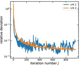
Figure 2: Measuring the convergence of the iterative solution technique to solve the chemistry with vertical mixing, here for the model with medium strong mixing, $\alpha_{\rm mix}\!=\!10^{-3}$. See text for explanations.

start of iterations	end of iterations

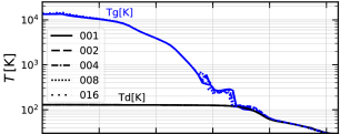
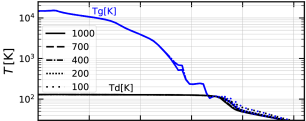
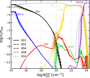
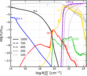
Figure 3: Monitoring the convergence of the iterative solution method along a vertical cut at $r\!=\!10\,$au as function of the vertical hydrogen nuclei column density $N_{\rm\langle H\rangle}\!=\!\int_{z}^{\infty}n_{\langle\rm H\rangle}(z)\,dz$ for the model with medium strong mixing $\alpha_{\rm mix}\!=\!10^{-3}$. The upper plots show the changing gas and dust temperature as function of iteration number. The lower plots shows the concentrations of a few selected oxygen-bearing gas and ice species. The left row shows the first few iterations, and the right row shows the convergence towards iteration 1000, which is considered as the final solution. The different full, dashed and dotted lines correspond to the different numbers of iterations carried out as indicated.

Figure 3 shows some details how the temperature and a few selected molecular concentrations change during the course of the iterations, considering a vertical cut through the disc at 10 au. We observe that the chemical structure changes considerably within the first few iterations, but then the changes per iteration settle down, and eventually the differences between iteration 400 (dash-dotted lines) and iteration 1000 (full lines) are barely recognisable on the right side of Fig. 3. The temperature structure also changes. The gas and dust temperatures cool down because (i) more OH and H2O form which lead to increased line cooling and (ii) the optical depths increase due to the presence of icy grains in upper regions. We conclude that our method does converge, albeit very slowly, which agrees with the expected convergence behaviour as discussed in Appendix A.4.

4.2 Impact on the chemical and temperature structure

$r\!=\!1\,$au	$r\!=\!10\,$au	$r\!=\!100\,$au

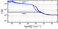
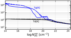
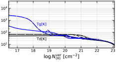
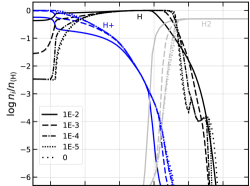
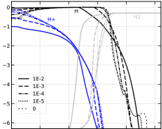
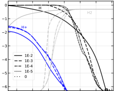
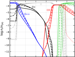
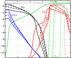
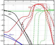
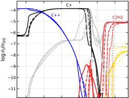
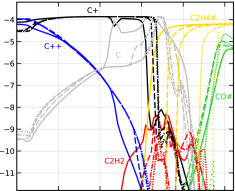
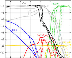
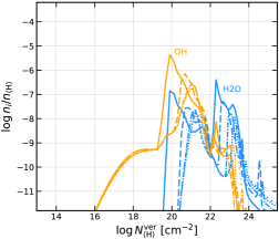
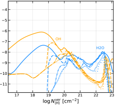
Figure 4: Resulting temperatures and chemical concentrations as function of vertical hydrogen column density $N_{\rm\langle H\rangle}$, for radial distances 1 au, 10 au, and 100 au, from left to right. The top row shows the gas and dust temperatures, the second row the main hydrogen species, the third row the oxygen chemistry, and the last row the carbon chemistry. Only a few selected species are plotted. In each part figure, the various dashed and dotted lines correspond to the mixing parameter $\alpha_{\rm mix}$ as explained in the legends.

4.2.1 Overview of principle effects

Figure 4 shows our resulting temperature and chemical structures. Each plot shows a sequence of well-iterated results for $\alpha_{\rm mix}\in\{0,10^{-5},10^{-4},10^{-3},10^{-2}\}$ using different line styles. The results are shown by three vertical cuts at constant distance to the star, at 1 au, 10 au and 100 au, each as function of hydrogen nuclei column density $N_{\rm\langle H\rangle}\rm\,[cm^{-2}]$.

The figure shows a number of remarkable changes of the chemical structure that are caused by the inclusion of vertical mixing, which will be detailed in the forthcoming sections.

• The ices that predominantly form in the midplane are mixed upward by a distance that corresponds to several orders of magnitude in column density.

• Molecules, which are mainly formed in the warm intermittent disc layers, where the temperatures are a few 100 K, are mixed both downward and upward.

• The increased molecular abundances of OH and H₂O cause reinforced line cooling at column densities $N_{\langle\rm H\rangle}$ $\sim$ $10^{19}...\,10^{22}\rm\,cm^{-2}$, which lowers the gas temperature and improves the conditions for the formation and survival of more molecules. These layers are the regions directly observable with infrared line spectroscopy. We see that the maximums of the OH and H₂O concentrations shift leftward and upward by about 1-2 orders of magnitude in these plots. These changes are larger for more distant regions and/or larger mixing parameter $\alpha_{\rm mix}$.

• Neutral atoms are mixed up into the highest layers, where they absorb X-rays and FUV radiation, which leads to additional absorption of UV and X-rays, causing an increase of temperature, and an increase of the shielding for the upper disc layers at larger radii.

• Ions such as O⁺, which are predominantly formed in high layers, are increasingly able to meet molecules and even icy grains which are mixed upward. This leads to a very rich ion-molecule chemistry, with new chemical pathways, that are normally unimportant in models without mixing.

4.2.2 Beating UV photo-desorption by mixing

$\alpha_{\rm mix}\!=\!0$	$\alpha_{\rm mix}\!=\!10^{-3}$	$\alpha_{\rm mix}\!=\!10^{-2}$

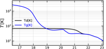
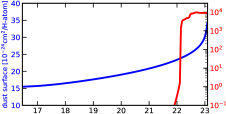
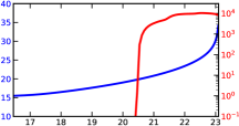
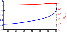
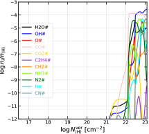
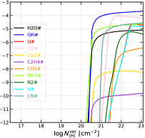
Figure 5: Vertical spreading of icy grains at $r\!=\!100\,$au for different mixing strengths $\alpha_{\rm mix}$. Results are shown as function of the vertical hydrogen nuclei column density $N_{\rm\langle H\rangle}$. The top row of plots shows the computed gas and dust temperatures, $T_{\rm g}$ and $T_{\rm d}$. The middle row of plots shows the bare grain surface area per H nucleus$\,=\!4\pi\langle a^{2}\rangle n_{d}/n_{\rm\langle H\rangle}$ after dust settling in blue, and the number of ice layers on each grain $N_{\rm layers}$ in red. The lower plots show the concentrations of selected ice species.

At large radial distances $\sim$ 100 au, the model with the highest mixing strength $\alpha_{\rm mix}\!=\!10^{-2}$ exhibits some rather peculiar results, see Fig. 5. The concentrations of the thermally most stable ice species such as H2O#, NH3#, CO2#, OH# and C2H4# (and some others not shown) become about constant and remain high even at the very top of the model, where they face the unattenuated stellar radiation field. This is in contrast to the less thermally stable ices such as CO# and N2# (and others).

In models without mixing, the ices are generally not stable in the optically thin disc regions because of UV photo-desorption. In the model with strong mixing $\alpha_{\rm mix}\!=\!10^{-2}$, however, the upward mixing rates seem to be large enough to replenish the ice species faster than the UV desorption can destroy them. This is in contrast to thermal desorption. Once the ices become thermally unstable, due to the increasing dust temperature in higher layers, they will sublimate very quickly and mixing cannot change that. We see this behaviour very clearly in the upper part of Fig. 8, where the upper boundary of CO# does not surpass the dust temperature $T_{\rm d}\!=\!25\,$K line, and the H2O# upper boundary does not surpass the $T_{\rm d}\!=\!150\,$K line, which corresponds to the desorption energies of these ices.

With an assumed stellar luminosity $L_{\star}\!=\!1\,L_{\odot}$ and $f_{\rm UV}\!=\!0.01$, we obtain a UV flux of about $6\times 10^{10}$ photons/cm²/s between 912Å and 2050Å at $r\!=\!100\,$au in the optically thin part high above the disc, which is about a factor of $\chi\!=\!300$ larger than the standard Draine flux in the ambient interstellar medium $F_{\rm Draine}\!=\!1.921\times 10^{8}\rm\ photons/cm^{2}/s$ (Draine & Bertoldi, 1996). With the symbols introduced in section 5 of Woitke et al. (2009), the UV photo-desorption rate of an ice species is

$$\frac{dn_{i\#}}{dt}=-\pi\langle a^{2}\rangle\,n_{d}\,Y_{i}\,\chi F_{\rm Draine}\times\left\{\begin{array}[]{cc}\displaystyle\frac{n_{i\#}}{n_{\rm act}}&,\ n_{\rm tot}^{\rm ice}<n_{\rm act}\\[8.53581pt] \displaystyle\frac{n_{i\#}}{n_{\rm tot}^{\rm ice}}&,\ n_{\rm tot}^{\rm ice}\geq n_{\rm act}\end{array}\right.\ ,$$ (29)

where $n_{d}$ is the number density of dust particles, $\pi\langle a^{2}\rangle n_{d}$ the total dust cross section per $\rm cm^{3}$, $Y_{i}$ the UV photo-desorption yield, and $n_{\rm act}=4\pi\langle a^{2}\rangle\,n_{d}\,2\,n_{\rm surf}$ is the total number of active adsorption sites on all grains per $\rm cm^{3}$. Following Aikawa et al. (1996), we assume that the uppermost two mono ice layers are active, meaning that frozen molecules can be hit directly by UV and can escape freely from these layers, with a surface density of $n_{\rm surf}\!=\!1.5\times 10^{15}$ sites per $\rm cm^{2}$ of solid surface.

The first case in Eq. (29) corresponds to a situation where the grain surface is almost unoccupied and the ratio $n_{i\#}/n_{\rm act}$ expresses the probability that a UV photon absorbed by a grain hits a site occupied by ice species $i$. In the second case, the surface is more than fully occupied and the ratio $n_{i\#}/n_{\rm tot}^{\rm ice}$ expresses the probability to find ice species $i$ in the ice mixture present, where the total ice density is $n_{\rm tot}^{\rm ice}=\sum_{i}n_{i\#}$. Hence, thick ice mantles can only be reduced layer by layer via photo-desorption, i.e. at a constant rate (“zero-order photo-desorption”). Figure 5 shows that, according to the assumed dust size distribution and dust/gas ratio, the grains in the midplane are covered by about $N_{\rm layers}=n_{\rm tot}^{\rm ice}/(4\pi\langle a^{2}\rangle n_{d}\,n_{\rm surf})\approx 10^{4}$ ice mono-layers.

The timescale to completely UV photo-desorb such grains in the optically thin upper disc layers can be obtained by summing up Eq. (29) over all ice species $i$, applying the second case

$$\tau_{\rm UVdesorb}=\frac{n_{\rm tot}^{\rm ice}/n_{\langle\rm H\rangle}}{\frac{\pi\langle a^{2}\rangle n_{d}}{n_{\langle\rm H\rangle}}\,\bar{Y}\,\chi F_{\rm Draine}}\approx\big{(}35000\,{\rm yrs}\big{)}\left(\frac{300}{\chi}\right)$$ (30)

where we have assumed a total initial ice concentration of $n_{\rm tot}^{\rm ice}/n_{\langle\rm H\rangle}\!\approx\!10^{-3.5}$, a mean photo-desorption yield of $\bar{Y}\!\approx\!10^{-3}$ and a total dust surface per H-atom of $4\pi\langle a^{2}\rangle n_{d}/n_{\langle\rm H\rangle}\!\approx\!2\times 10^{-23}\rm\,cm^{2}$ (compare Fig. 5). We note that $\chi\!\approx\!300$ is what we find in our model at $r\!=\!100\,$au. $\chi\propto 1/r^{2}$ (i.e. $\tau_{\rm UVdesorb}\propto r^{2}$) is valid until the interstellar UV photons become more relevant than the diluted stellar UV, which happens at about 1700 au in this case.

In comparison, the turbulent eddy-diffusion timescale is

$$\tau_{\rm mix}=\frac{H_{p}}{\alpha_{\rm mix}c_{s}}\approx\big{(}18000\,{\rm yrs}\big{)}\left(\frac{r}{100\,{\rm au}}\right)^{1.4}\left(\frac{10^{-2}}{\alpha_{\rm mix}}\right)$$ (31)

where we assumed a scale height of $H_{p}\!=\!({\rm 10\,au})(r/{\rm 100\,au})^{1.15}$, a temperature structure as $T=({\rm 20\,K})(r/{\rm 100\,au})^{-0.5}$, a constant mean molecular weight of $\mu\!=\!2.3\,$amu, and $c_{s}\!=\!\sqrt{kT/\mu}$.

$\alpha_{\rm mix}\!=\!0$	$\alpha_{\rm mix}\!=\!10^{-3}$

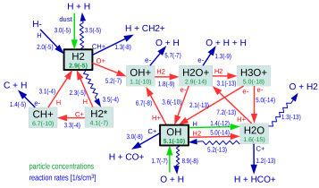
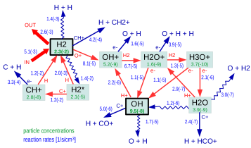
Figure 6: Chemical pathways to create OH and H2O molecules without mixing (left) and with $\alpha_{\rm mix}\!=\!10^{-3}$ (right) at one selected point in the disc at $r\!=\!10\,$au located in the upper disc layers, see text. The green numbers represent the particle concentrations and the blue numbers the rates $\rm[cm^{-3}s^{-1}]$ in the time-independent case. The big red “IN” and “OUT” arrows on the right denote the in-mixing and out-mixing rates for H2. Wiggled arrows indicate photo-dissociation. Light green arrows on the left mark the H2-formation on grains and the radiative association reactions  ${\rm O+H\to OH}+h\nu$  and  ${\rm OH+H\to H_{2}O}+h\nu$.  $\rm H_{2}^{\star}$ denotes electronically excited molecular hydrogen. The figure does not follow up the production of CH2+, CO+ and HCO+ marked in blue. The notation $a(-b)$ means $a\times 10^{\,-b}$.

The conclusion from this timescale comparison is that only for very large $\alpha_{\rm mix}$ and large radii, the up-mixing of icy grains can indeed be faster than UV desorption. The two timescales meet at about 30 au in our model with $\alpha_{\rm mix}\!=\!10^{-2}$, which is in agreement with where we start to see icy grains in the uppermost disc layers in our models. In all other cases, the icy grains stay confined to the midplane due to UV photo-desorption. However, the vertical spread of the icy grains is distinctively wider as compared to un-mixed models, and strongly depends on parameter $\alpha_{\rm mix}$. The entirely flat concentrations of the most stable ices in the $\alpha_{\rm mix}\!=\!10^{-2}$ model are still somewhat surprising. Possibly, the strong increase of the gas temperature, from a few 10 K to a few 100 K, causing larger $c_{s}$ and hence shorter mixing timescales, is responsible for this behaviour.

4.2.3 Chemical pathways

In order to better understand the chemical processes induced by mixing, let us examine one point in our disc model with $\alpha_{\rm mix}\!=\!10^{-3}$ at 10 au, located at the maximum of the concentration of OH, that is the maximum of the red curve in Fig. 3 (right part) at $N_{\rm\langle H\rangle}\!\approx\!1(+20)\rm\,cm^{-2}$. The notation $a(+b)$ means $a\times 10^{+b}$. Here we have a hydrogen nuclei density of $n_{\langle\rm H\rangle}\!=\!2.4(+7)\rm\,cm^{-3}$. The gas and dust temperatures are $T_{g}\!=\!347\,$K and $T_{d}\!=\!126\,$K, and the point is optically thin with radial and vertical visual extinctions $A_{V}^{\rm rad}\!=\!0.024$ and $A_{V}^{\rm ver}\!=\!6.3(-4)$, respectively. The most abundant (“available”) species are H $[9.5(-1)]$, H2 $[2.3(-2)]$, O $[3.0(-4)]$, e- $[1.5(-4)]$, C+ $[1.3(-4)]$, N $[7.9(-5)]$, and H+ $[2.1(-5)]$, where the numbers in squared brackets are the concentrations $n_{i}/n_{\langle\rm H\rangle}$.

Figure 6 shows how the up-mixing of H2 fuels the ion-neutral chemistry in the upper disc regions, resulting in an enhanced production of OH and H2O. The left side of the figure shows the rates and concentrations in the case without mixing, where OH is mainly produced via the radiative association reaction ${\rm O+H\to OH}+h\nu$, water is mainly produced by the follow-up radiative association reaction ${\rm OH+H\to H_{2}O}+h\nu$, and H2 is produced partly by the formation on grains and partly via $\rm H+H^{-}\to H_{2}+e^{-}$.

On the right side of Fig. 6, which shows the results at the same point for the case with mixing $\alpha_{\rm mix}\!=\!10^{-3}$, the H2-concentration is enhanced by a factor of about 1000. Here, the starting point for the production of OH and H2O is the reaction

$$\rm H_{2}\leavevmode\nobreak\ +\leavevmode\nobreak\ O^{+}\leavevmode\nobreak\ \longrightarrow\leavevmode\nobreak\ OH^{+}\leavevmode\nobreak\ +\leavevmode\nobreak\ H\ ,$$ (32)

where the O+ is produced by charge exchange with H+, which results from secondary X-ray reactions with super-thermal electrons $\rm H+e^{-}\to H^{+}+e^{-}+e^{-}$. Although reaction (32) is only the forth most important destruction reaction of H2 (after out-mixing, photo-dissociation and reaction with CH+), it triggers the production of OH and H2O via the formation of OH+. Quick H-addition reactions with H2 subsequently produce H2O+ and H3O+, before recombinations with free electrons create the neutral molecules OH and H2O. This H2O formation path is nomally initiated by reactions of O with H3+, for example $\rm O+H_{3}^{+}\to OH^{+}+H_{2}$, but here we find reaction (32) to be more efficient in producing OH+, because the mixing leads to a coexistence of H2 and O+. Since H2 is required several times along these formation pathways, even a small increase of the H2 concentration, caused by up-mixing, can lead to a much higher production of OH and H2O molecules. The resulting OH and H2O concentrations are higher by about 2.5 and 6 orders of magnitude, respectively, at this point, when mixing is taken into account with $\alpha_{\rm mix}\!=\!10^{-3}$. The reaction cycles are completed by photo-dissociation and dissociative recombination reactions, which again destroy the molecules and replenish the atoms.

Noteworthy, H2 is the only molecule that is strongly affected by mixing directly in Fig. 6. All other molecules shown in Fig. 6 have the same reaction coefficients for the MI and MO quasi reactions, yet their low concentrations render these rates insignificant. The only other species directly affected by mixing are those atoms and ions listed as “abundant” in the beginning of this paragraph. This finding can be explained by considering the chemical formation/destruction timescales (particle densities over rates). For low-abundance molecules, particle densities are low but rates are similar, i.e. the chemical timescales are short. Only for the most abundant molecules the chemical timescale can exceed the mixing timescale. The other species with low abundances and short chemical timescales tend to rather adjust their concentrations quickly to these changed circumstances.

$\alpha_{\rm mix}\!=\!0$	$\alpha_{\rm mix}\!=\!10^{-3}$

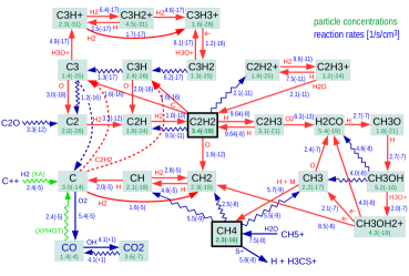
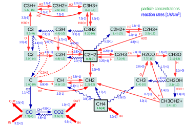
Figure 7: Chemical pathways to create C2H2 and other hydro-carbon molecules without mixing (left) and with $\alpha_{\rm mix}\!=\!10^{-3}$ (right) at one selected point in the disc at $r\!=\!0.15\,$au, see text. Note the vastly different concentrations of all hydro-carbon molecules. As in Fig. 6, the green numbers represent the particle concentrations and the blue numbers the rates $\rm[cm^{-3}s^{-1}]$ in the time-independent case. The big red “IN” and “OUT” arrows denote the in-mixing and out-mixing rates. Wiggled arrows indicate photo-dissociation. The light green wiggled arrows are X-ray induced processes. Three reactions appear twice with an added dashed line, when a reaction is important for two reactants or products ($\rm C_{2}H_{2}+C\to C_{3}+H_{2}$, $\rm C_{2}H_{2}+C\to C_{3}H+H$ and ${\rm C_{3}}+h\nu\to\rm C_{2}+C$). On the left side, the reaction paths for C2O, C++, CH5+ and H3CS+ are not followed up.

Next, we have a look at the hydro-carbon chemistry. We consider a point in our $\alpha_{\rm mix}\!=\!10^{-3}$ disc model at $r\!=\!0.15\,$au, at a height where the C2H2 concentration is steeply rising towards a plateau in the midplane, that is at a vertical hydrogen column density of about $N_{\rm\langle H\rangle}\!\approx\!1.0(+23)\rm\,cm^{-2}$ on the left plot in Fig. 4. Points like these are flagged by ProDiMo as the main emission region for the C2H2 13.7 $\mu$m emission feature observable with Spitzer/IRS and JWST/MIRI, see Fig. 10. Here, we have a hydrogen nuclei density of $n_{\langle\rm H\rangle}\!=\!1.0(+13)\rm\,cm^{-3}$, the gas and dust temperatures are $T_{g}\!=\!353\,$K and $T_{d}\!=\!354\,$K, and the point is optically thick in the radial direction, $A_{V}^{\rm rad}\!=\!194$, but semi optically thin in the vertical direction, $A_{V}^{\rm ver}\!=\!3.1$, still resulting in a total UV strength of $\chi\!=\!20000$. The most abundant species are H2 $[0.5]$, H $[5.6(-3)]$, H2O $[1.7(-4)]$, CO $[1.3(-4)]$, and N2 $[3.6(-5)]$, no ices.

Figure 7 shows how the up-mixing of CH4 followed by photo-dissociation leads to much higher concentrations of all hydro-carbon molecules. The hydro-carbon chemistry forms an almost self-contained reaction sub-system that is only weakly connected to other chemicals. Comparing the two depicted cases (with and without mixing), we see that the same neutral-neutral, ion-neutral and photo-dissociation reactions connect the different hydro-carbon species in similar ways, forming sustained reaction cycles. The various reactions with O or O2 in these cycles form C-O bonds that, once formed, can hardly be destroyed again. We will denote these oxidisation reactions as “burning” in the following. On the left side of Fig. 7 (without mixing) these reactions consume almost all hydro-carbon molecules, until an equilibrium with neutral carbon atoms is established, on a very low level $n_{\rm C}/n_{\langle\rm H\rangle}\!=\!3(-14)$, where further burning of the H–C molecules is balanced by X-ray destruction of CO and X-ray induced charge exchange (XA) with C++.

On the right side of Fig. 7 (with mixing), methane molecules (CH4) that formed further down in the UV-protected disc layers are mixed up into the semi optically thin region considered here, where they are quickly photo-dissociated as

$${\rm CH_{4}}\leavevmode\nobreak\ +\leavevmode\nobreak\ h\nu\leavevmode\nobreak\ \longrightarrow\leavevmode\nobreak\ \left\{\begin{array}[]{lc}\rm CH_{3}\leavevmode\nobreak\ +\leavevmode\nobreak\ H&(15.5\%)\\ \rm CH_{2}\leavevmode\nobreak\ +\leavevmode\nobreak\ H_{2}&(69.0\%)\\ \rm CH\leavevmode\nobreak\ +\leavevmode\nobreak\ H_{2}\leavevmode\nobreak\ +\leavevmode\nobreak\ H&(15.5\%)\end{array}\right.$$ (33)

with branching ratios from the UMIST 2012 database (McElroy et al., 2013). This introduces rates of the order of $\rm 10^{-1}\,cm^{-3}\,s^{-1}$ to the hydro-carbon system. The system reacts to this input by increasing all concentrations of hydro-carbon molecules by many orders of magnitude, from about 4 decades for C to 15 decades for C3H. The concentration of acetylene (C2H2), which results to be the most abundant hydro-carbon molecule in this case, increases from $3.4(-19)$ to $8.3(-7)$, creating a peculiar chemical situation where carbon can be found in opposite redox states (C2H2 and CO2) in similarly high concentrations.

Again, only the abundant molecules shown with big red arrows in Fig. 7 (CO, CO2 and CH4) are significantly affected by mixing directly. All other molecules just adjust to those circumstances quickly. For example, C2H2 has a chemical relaxation timescale of about $n_{\rm C2H2}/{\rm rate}\approx\rm 8(-7)\times 1(+13)\,cm^{-3}/(3(+4)\,cm^{-3}s^{-1})=270\,$s at this point, which is much shorter than the mixing timescale $\approx\rm\!2\,yrs$ (Eq. 30).

In summary, the CH4 molecules that are mixed up from deeper layers by eddy-diffusion are quickly photo-dissociated once they reach the borderline optically thin layers. The products of these photo-processes react further to create a rich hydro-carbon chemistry in an oxygen-rich situation, where the various hydro-carbon molecules are ultimately burnt on timescales of a few years at $r\!=\!0.15\,$au, forming C-O bonds. We actually see in Fig. 7 that there is an over-production of CO and CO2 that is mixed out.

5 Impact on continuum and line observations

In this section, we demonstrate how turbulent mixing can affect continuum and line observations. The impact is generally quite substantial, and we have selected to demonstrate three of the mayor effects in this paper. We do not intend to make any predictions for particular targets in this paper.

5.1 Impact on spectral ice features

$\alpha_{\rm mix}=0$	$\alpha_{\rm mix}=10^{-5}$	$\alpha_{\rm mix}=10^{-4}$	$\alpha_{\rm mix}=10^{-3}$	$\alpha_{\rm mix}=10^{-2}$

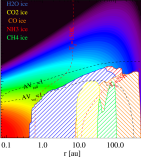
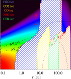
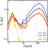
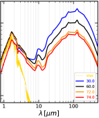
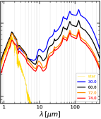
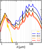
Figure 8: The upper row of plots shows the location of the ices, in a series of models with increasing mixing parameter $\alpha_{\rm mix}$. The icy regions are hashed when the respective ice concentration, for example $n_{\rm H2O\#}/n_{\langle\rm H\rangle}$ for water ice, is larger than $10^{-5.5}$. The background colours show the hydrogen nuclei density $n_{\rm\langle H\rangle}$ from $10^{\,2}\rm\,cm^{-3}$ (black) to $10^{\,16}\rm\,cm^{-3}$ (red). The black dashed contour lines show the radial visual extinction $A_{V,\rm rad}\!=\!1$ and vertical visual extinction $A_{V,\rm ver}\!=\!1$, and the red dashed lines show two dust temperature contours, 25 K and 150 K. The lower row of plots shows the respective spectral energy distributions (SEDs) for selected inclination angles at a distance of 140 pc. The yellow lines indicates the adopted photospheric spectrum of the naked star. We note that the absorption feature around 2.5 $\mu$m is due to molecular absorption in the stellar photosphere, whereas all other narrow absorption and emission features are due to ices, beside the broad 10$\,\mu$m / 20$\,\mu$m silicate emission features.

In our models, the up-mixing of icy grains leads to a substantial increase of the ice concentrations in the observable disc surface, see details in Sect. 4.2.2. Figure 8 shows the spatial distribution of five selected ice species (H2O #, NH3 #, CO2 #, CO #, and CH4 #) in the entire disc. In the un-mixed case, most ices only populate the midplane regions below $A_{\rm V,ver}\!\approx\!10$, due to active UV photo-desorption in the upper disc regions. The only counter-example is CO # in the outer regions $\mathrel{\mathchoice{\vbox{\offinterlineskip\halign{\hfil$\displaystyle#$\hfil\cr>\cr\sim\cr}}}{\vbox{\offinterlineskip\halign{\hfil$\textstyle#$\hfil\cr>\cr\sim\cr}}}{\vbox{\offinterlineskip\halign{\hfil$\scriptstyle#$\hfil\cr>\cr\sim\cr}}}{\vbox{\offinterlineskip\halign{\hfil$\scriptscriptstyle#$\hfil\cr>\cr\sim\cr}}}}\!100\,$au, but this region is too cold to cause any significant far-IR ice emission features. Since the spectral energy distribution (SED) is mostly produced by thermal emission and scattering of the bare (i.e. ice-less) dust grains above $A_{\rm V,ver}\!=\!10$, the resulting SED is almost entirely free of ice features, also at grazing inclination angle ($\approx\!72^{\rm o}$ in this model), which tests the $A_{\rm V,rad}\!\approx\!1$ regions in absorption. The ice just sits too deep to cause any notable changes of the integrated spectral flux. One would need to observationally search for the ice features by analysing image data, using the intensities coming from the dark lane, see discussion in Arabhavi et al. (2022).

However, even a weak turbulent mixing with $\alpha_{\rm mix}\!=\!10^{-5}$ lifts some of the icy grains upwards, almost reaching the $A_{\rm V,ver}\!=\!1$ surface, and some weak ice emission features between 20 $\mu$m and 200 $\mu$m start to appear in the spectrum, which become more clearly observable in the $\alpha_{\rm mix}\!=\!10^{-4}$ model. We also see that the $A_{\rm V,ver}\!=\!1$ contour moves upwards with increasing $\alpha_{\rm mix}$ due to the opacity of the icy grains. So, scattered starlight can now directly interact with the icy grains.

At $\alpha_{\rm mix}\!=\!10^{-3}$, the ice emission features become even stronger, and the icy grains reach the $A_{\rm V,rad}\!=\!1$ line, i.e. direct starlight can now interact with icy grains. The first three ice absorption features appear when the disc is observed under an inclination angle of $\approx\!74^{\rm o}$.

Eventually, the extreme model with $\alpha_{\rm mix}\!=\!10^{-2}$ shows a population of H2O # and NH3 # up to the very top of the model, accompanied by another considerable lift of the $A_{\rm V,ver}\!=\!1$ and $A_{\rm V,rad}\!=\!1$ contours. We note that the vertical extension of the snowy grains coincides with the dust temperature $T_{\rm dust}\!=\!150\,$K contour, which means that the snow extends right up to the water ice sublimation temperature in this model, whereas the UV photo-desorption becomes an irrelevant process, see explanations in Sect. 4.2.2. The same is true for the vertical extension of CO # at larger radial distances, which is limited by the $T_{\rm dust}\!=\!25\,$K contour. The SED is full of strong ice emission features, and clear absorption features for inclination angles $\mathrel{\mathchoice{\vbox{\offinterlineskip\halign{\hfil$\displaystyle#$\hfil\cr>\cr\sim\cr}}}{\vbox{\offinterlineskip\halign{\hfil$\textstyle#$\hfil\cr>\cr\sim\cr}}}{\vbox{\offinterlineskip\halign{\hfil$\scriptstyle#$\hfil\cr>\cr\sim\cr}}}{\vbox{\offinterlineskip\halign{\hfil$\scriptscriptstyle#$\hfil\cr>\cr\sim\cr}}}}\!72^{\rm o}$. We note that the strengths of the ice features depends on how we assume the ices to be distributed onto the pre-existing bare grains, and our assumption of a layer of equal thickness on top of each refractory grain creates the strongest ice opacities, see discussion in Arabhavi et al. (2022).

5.2 Impact on mid-IR gas emission line spectra

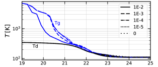
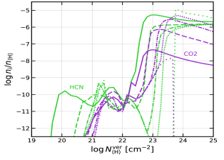
Figure 9: Gas and dust temperatures (upper panel), and concentrations of selected IR active molecules (lower panels) along a vertical cut at $r\!=\!1$ au as function of vertical hydrogen nuclei column density $N_{\rm\langle H\rangle}$. The results of five models are overplotted using different line styles, from $\alpha_{\rm mix}\!=\!0$ to $10^{-2}$, see top panel.

Figure 9 shows the dust and gas temperatures, and the concentrations of the IR-active molecules OH, H2O, CO2, HCN, C2H2 along a vertical cut at $r\!=\!1$ au. We see that all molecules shift their location of maximum concentration to the left, i.e. upwards towards smaller column densities, but whereas OH, H2O, HCN and C2H2 are enhanced by mixing, CO2 is reduced. This is because of the upmixing of CH4 which leads to a rich hydro-carbon chemistry as discussed in Sect. 4.2.3, which suppresses the formation of CO2. The figure also shows that the gas in the upper layers cools down via increased line emission from OH and H2O, the concentrations of which are enhanced by mixing.

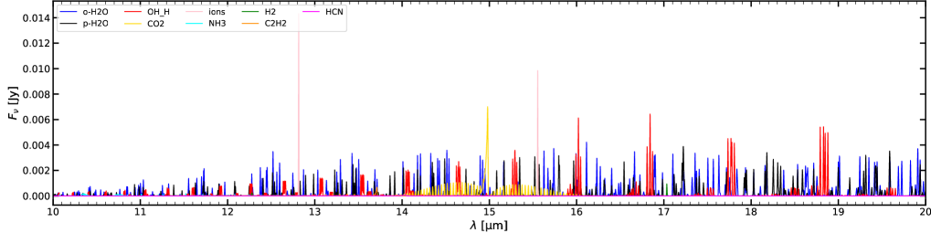
$\boxed{\alpha_{\rm mix}\!=\!0}$

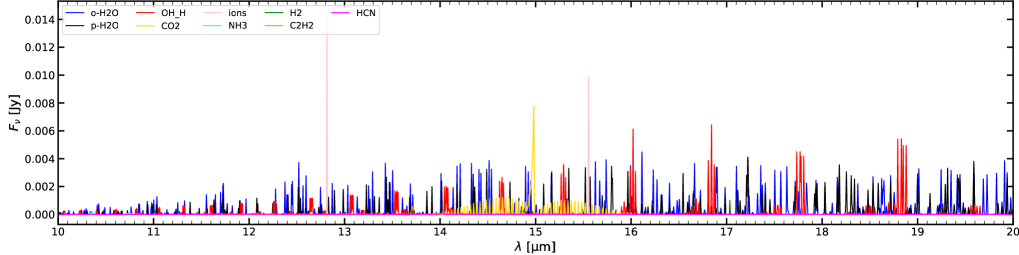
$\boxed{\alpha_{\rm mix}\!=\!10^{-5}}$

$\boxed{\alpha_{\rm mix}\!=\!10^{-4}}$

$\boxed{\alpha_{\rm mix}\!=\!10^{-3}}$

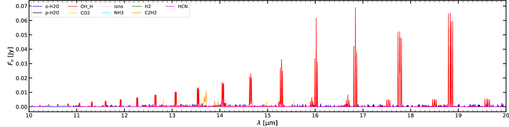
$\boxed{\alpha_{\rm mix}\!=\!10^{-2}}$

Figure 10: Continuum-subtracted infrared line emission spectra for disc inclination $45^{\rm o}$ and spectral resolution $R\!=\!3000$ with varying mixing parameter $\alpha_{\rm mix}$. Note the different scaling of the $y$-axis. Most visible spectral features are overlapping o-H2O (blue) and p-H2O (black) emission lines. A few other features emitted from other molecules and ions are annotated in one of the plots. Each molecular spectrum is first convolved with a Gaussian $R\!=\!3000$ and then overplotted with a certain colour, but not co-added.

$\alpha_{\rm mix}=0$	$\alpha_{\rm mix}=10^{-4}$	$\alpha_{\rm mix}=10^{-2}$

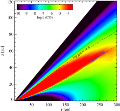
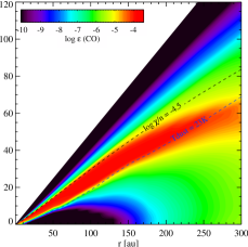
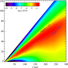
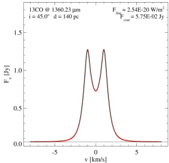
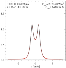
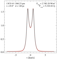
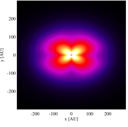
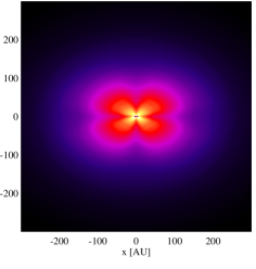
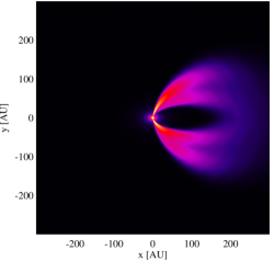
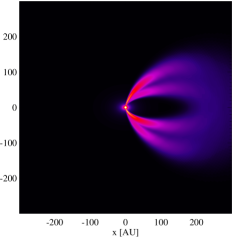
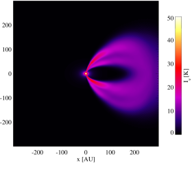
Figure 11: Influence of vertical mixing on millimetre CO observations. The top row shows the CO concentration $\epsilon({\rm CO})\!=\!n_{\rm CO}/n_{\langle\rm H\rangle}$ in the disc on linear scales for radius $r$ and vertical height $z$. The two dashed contour lines enclose the region of maximum CO concentration, where $\chi$ is the UV strength and $n=n_{\langle\rm H\rangle}$ is the total hydrogen nuclei particle density. Below dust temperature $T_{\rm dust}\!\approx\!23\,$K, CO is mostly frozen. The second row shows the ¹³CO J$=2\!\to\!1$ line velocity profile observed from a distance of 140 pc at disc inclination $45^{\rm o}$. The third row shows the integrated line map after continuum subtraction and the bottom row shows a channel map at radial velocity $v+0.94\,$km/s. To plot the intensities in Kelvin, we consider $I_{\nu}\,c^{2}/(2\nu^{2})/k$, where $I_{\nu}\rm\,[erg/cm^{2}/s/Hz/sr]$ is the spectral intensity, $c$ the speed of light, $\nu$ the frequency and $k$ the Boltzmann constant.

Figure 10 shows a series of mid-IR gas emission line spectra between 10 $\mu$m and 20 $\mu$m computed from our series of T Tauri disc models with $\alpha_{\rm mix}\!=\!0$ to $10^{-2}$, see Sect. 3 These spectra have been calculated with the Fast Line Tracer FLiTs developed by Michiel Min (see Woitke et al., 2018) on top of the gas & dust temperature structure, the continuum dust opacities, the molecular abundances and the non-LTE excitation populations calculated by ProDiMo as described in the previous sections. Due to our lack of sufficient collisional data, the populational numbers of the molecules OH, CO2, HCN, C2H2 and NH3 are assumed to be in LTE. FLiTs calculates the entire spectrum on a wavelength grid that corresponds to a velocity resolution of 1 km/s. We have calculated the spectra separately for each molecule listed in the legend of Fig. 10. In contrast, the IR lines of the atoms and ions Ne+, Ne++, Ar+, Ar++, Mg+, Fe+, Si+, S, S+ and S++ are calculated in one go. For more details and explanations, see Woitke et al. (2018). The resulting continuum-subtracted spectra are then convolved with a $R\!=\!3000$ Gaussian before plotting, to simulate the spectra that we can expect from JWST/MIRI.

As discussed in Woitke et al. (2018), these predicted spectra are broadly consistent with Spitzer/IRS observational data of T Tauri stars concerning line colours and ratios. However, since we assumed a dust/gas ratio of 100 here, instead of 1000 in this paper, and since we only applied a very mild dust settling with $\alpha_{\rm settle}\!=\!10^{-2}$ according to Dubrulle et al. (1995), the dust is still covering most of the line emitting regions, and the predicted IR lines are generally too weak, by a factor of about 10-100. It also means that the lines that are emitted from higher disc layers (e.g. by Ne+ and OH) are stronger than those emitted from lower layers (e.g. H2O, HCN and C2H2). Therefore, we can only discuss the trends here that are caused by the introduction of mixing.

We see little changes between $\alpha_{\rm settle}\!=\!0$ and $\alpha_{\rm settle}\!=\!10^{-4}$. Only at $\alpha_{\rm settle}\!=\!10^{-3}$, the OH lines start to become significantly stronger, and the C2H2 and HCN emission features at 13.7 $\mu$m and 14 $\mu$m, respectively, start to be enhanced and become about comparable to the CO2 feature at 15 $\mu$m, as is observed for many T Tauri stars (Pontoppidan et al., 2010). For $\alpha_{\rm settle}\!=\!10^{-2}$, the OH lines become too strong with respect to the H2O lines, similar to the findings of Heinzeller et al. (2011). C2H2 13.7 $\mu$m is now the strongest spectral feature between 10 $\mu$m and 20 $\mu$m after the various OH ro-vibrational features, which is also in disagreement with Spitzer observations.

5.3 Impact on CO lines and channel maps

The upper row of Fig. 11 shows the resulting CO concentration on linear radial and vertical scales in the same model series. In our disc models, carbon results to be mostly present in form of CO, with a maximum concentration of $n_{\rm CO}/n_{\langle\rm H\rangle}\!\approx\!\epsilon_{\rm C}\!=\!10^{\,-3.85}$, in a vertical layer that is limited by photo-dissociation on top (ionisation parameter $\chi/n_{\langle\rm H\rangle}\!\approx\!10^{\,-4.5}$) and by ice formation at the bottom ($T_{\rm dust}\!\approx\!23\,$K). The ¹³CO $J\!\!=\!2\!\to\!1$ line at 1360.2 $\mu$m is mostly emitted from this vertical layer, and 70% of the line flux is emitted radially from about 50 au to 200 au in the disc model with $\alpha_{\rm mix}\!=\!0$. Beyond about 250 au the line becomes optically thin. Figure 11 shows the resulting line fluxes and double-peaked velocity profiles, the velocity-integrated line maps, and selected channel maps in the lowest panel.

We see two major effects of the mixing on the spectral appearance of the CO in millimetre lines. First, the CO line emission becomes weaker with increasing $\alpha_{\rm mix}$ at small radii. Figure 4 shows that at 100 au (right column) the disc cools down slightly with increasing $\alpha_{\rm mix}$. This is because of the additional presence of icy grains in higher disc layers due to mixing, see Sect. 4.2.2. Because of their enhanced opacity, the icy grains increase the vertical optical depths and also scatter away the starlight more efficiently. As a consequence, the height below which CO freezes out increases, and hence the vertical CO column density decreases. Figure 11 shows a clear trend of the CO emissions from the inner disc regions becoming weaker with increasing $\alpha_{\rm mix}$, see line maps, while the vertical layer of maximum CO concentration becomes thinner, see concentrations.

Second, the CO line emissions intensify with increasing $\alpha_{\rm mix}$ at large radii. This is a direct consequence of downward CO mixing. For large $\alpha_{\rm mix}$ the CO mixing timescale becomes shorter than the ice adsorption timescale in the outer regions, which leads to a more gradual decline of the CO concentration towards the midplane, and hence larger CO column densities in the outermost disc regions. The lower boundary of the vertical layer of maximum CO concentration becomes less well defined for large $\alpha_{\rm mix}$. This leads to a more “diffuse” spectral appearance in millimetre CO channel maps, see lower row of plots in Fig. 11. Without mixing, we obtain clearly separated line emissions from two lobes, one from the upper disc half, and one from the lower disc half. With strong mixing $\alpha_{\rm mix}\!=\!10^{-2}$, the two lobes visually merge beyond about 150 au. Cleeves et al. (2016) and Pinte et al. (2018) noticed that for the case of the giant disc of IM Lupi, where the CO lines are detectable out to $\sim\!1000$ au, it becomes impossible to identify two separate CO layers beyond $\sim\!450$ au. Pinte et al. (2018) achieved a distinctively better fit when adding diffuse CO emission from the outer midplane. We note, however, that even without mixing, the CO concentration in the midplane increases with radius as the freeze-out timescale of CO increases with falling density whereas the photo-dissociation timescale is density-independent.

In the model with the strongest mixing $\alpha_{\rm mix}\!=\!10^{-2}$, we furthermore observe that the CO is also vertically more extended toward to top. This is partly caused by an upward shift of the $\chi/n\!=\!10^{-4.5}$ contour line due to the increased dust opacities of the icy grains, but at the very top, the CO is actually mixed up quicker than it can be photo-dissociated. In summary, we confirm the finding of Semenov et al. (2006) that the CO density can be enhanced by mixing above and below the layer of maximum concentration, but we disagree with Semenov & Wiebe (2011) that the CO is not responsive to mixing.

6 Summary and Conclusions

6.1 Summary of chemical mechanisms

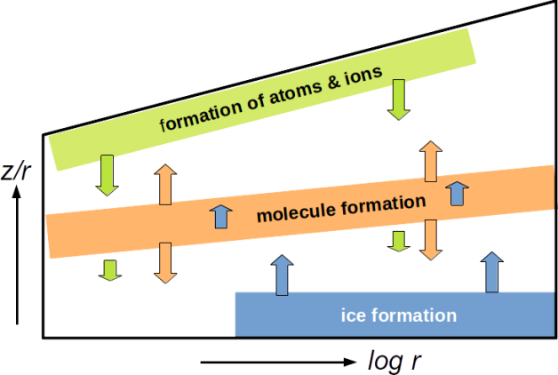
Figure 12: Schematic sketch of the disc regions responsible for the formation of atoms, molecules and ices, and their vertical diffusive transport.

Figure 12 summarises the principle mechanisms that we have identified in our disc models by means of a physical sketch. The mixing is immediately relevant for the most abundant species, such as H2, CH4, CO, the neutral atoms in higher layers, and the ices in the midplane. With “immediately relevant”, we mean that the transport rates can locally dominate over the chemical formation and destruction rates. The abundant species, whose concentrations are limited by element abundance constraints, are transported away from their regions of maximum concentration, both up and down, and in the locations where these abundant chemicals are finally destroyed, for example by photo-reactions, their reaction products fuel the local chemistry. The release of these fragments has important consequences for all other, chemically interlinked but less abundant molecules, which quickly adjust their concentrations to these changed circumstances. This generally creates a more active chemistry, with a richer mixture of ionised, atomic, molecular and ice species and new chemical pathways that are not relevant in the un-mixed case.

This situation differs somewhat from exoplanet atmospheres as e.g. discussed by Moses et al. (2011), Zahnle et al. (2016) and Barth et al. (2021). In exoplanet atmospheres, the chemical factories are located in the deepest layers, where temperatures and densities are high. From there, molecules are mixed upward, resulting in constant concentrations at intermediate heights, until photo-dissociation destroys them at high altitudes. In discs, the main chemical factories are located in the warm intermediate layers. From there, molecules are mixed upwards and downwards. The dense midplane is too cold to have an active chemistry. Instead, molecules freeze out there, and the icy grains are mixed up.

6.2 Summary of impact on spectral observations

Concerning the mid-IR molecular spectra, we see increased molecular abundances in the upper layers observable with Spitzer and JWST, in particular for OH, H2O, HCN and C2H2 in our models when we include mixing. The chemical response to mixing in these layers happens on short timescales, of the order of hours or days, and liberates more heat via exothermic reactions. However, at the same time the increased abundances of the IR active molecules lead to increased line cooling and a decrease of gas temperatures in those high layers. Despite the strong effects on both molecular abundances and gas temperature structure, the calculated IR spectra are surprisingly robust. We need to assume strong mixing $\alpha_{\rm mix}\!\mathrel{\mathchoice{\vbox{\offinterlineskip\halign{\hfil$\displaystyle#$\hfil\cr>\cr\sim\cr}}}{\vbox{\offinterlineskip\halign{\hfil$\textstyle#$\hfil\cr>\cr\sim\cr}}}{\vbox{\offinterlineskip\halign{\hfil$\scriptstyle#$\hfil\cr>\cr\sim\cr}}}{\vbox{\offinterlineskip\halign{\hfil$\scriptscriptstyle#$\hfil\cr>\cr\sim\cr}}}}\!10^{-3}$ to produce notable spectral changes. The spectral features of OH, HCN and C2H2 are enhanced by mixing, whereas the CO2 feature at 15 $\mu$m is reduced.

Concerning the CO millimetre emission lines, mixing reduces the line intensities at small radii but enhances them at larger radii, leading to an overall more flat line intensity profile in ALMA line observations. For intense mixing, CO starts to populate the outer midplane regions, which leads to a distinct, more diffuse appearance of the CO in velocity channel maps. However, it is likely that such differences in CO channel maps can also be produced in alternative ways in our models, for example by changing the column density profile $N_{\rm\langle H\rangle}(r)$ of the disc.

6.3 Conclusions about the $\alpha$ viscosity parameter

The parameter $\alpha_{\rm mix}$ describes the strength of the vertical turbulence according to the Shakura & Syunyaev (1973) $\alpha$-model. Our mixed models with $\alpha_{\rm mix}\!\mathrel{\mathchoice{\vbox{\offinterlineskip\halign{\hfil$\displaystyle#$\hfil\cr>\cr\sim\cr}}}{\vbox{\offinterlineskip\halign{\hfil$\textstyle#$\hfil\cr>\cr\sim\cr}}}{\vbox{\offinterlineskip\halign{\hfil$\scriptstyle#$\hfil\cr>\cr\sim\cr}}}{\vbox{\offinterlineskip\halign{\hfil$\scriptscriptstyle#$\hfil\cr>\cr\sim\cr}}}}\!10^{-3}$ show strong ice emission features between 20 $\mu$m and 200 $\mu$m, which neither Spitzer nor Herschel have seen for T Tauri stars. However, the $\alpha_{\rm mix}\!\approx\!10^{-5}$ and $10^{-4}$ models predict weak ice features that might require the signal/noise ratio of JWST to be detectable. Without mixing, it would be difficult to explain such detections with our models.

Concerning the mid-IR molecular emission lines, our models with $\alpha_{\rm mix}\!\approx\!10^{-3}$ predict more equal strengths of the CO2, HCN and C2H2 features between 13.7 $\mu$m and 15 $\mu$m, which is difficult to achieve in our models otherwise. However, for $\alpha_{\rm mix}\!\approx\!10^{-2}$, the OH and C2H2 emission features become unrealistically strong.

The detection of layered CO emission in ALMA channel maps, in form of two distinct lobes emitted by the lower and the upper disc halves, with no direct emission from the in-between midplane, allows us to put some constraint on the $\alpha$ viscosity parameter, because for large $\alpha_{\rm mix}$, CO would be expected to populate the midplane. However, that constraint is weak, about $\alpha_{\rm mix}\!<\!10^{-2}$.

We conclude that models with a modest choice of $\alpha_{\rm mix}\!\approx\!10^{-5}$ to $10^{-3}$ might work best to produce realistic continuum and line observations. However, a constant value of $\alpha_{\rm mix}$ is certainly unrealistic in the first place, as the turbulence is expected to vary with distance and height, see e.g. figure 9 of Thi et al. (2019).

Appendix A Numerical implementation of mixing

A.1 Numerical scheme

Let us consider height grid points $\{z_{k}\,|\,k=1,...,K\}$. The basic reaction-diffusion equation (Eq. 1) is numerically discretised as

$$\frac{\partial n_{i,k}}{\partial t}=P_{i,k}-L_{i,k}-\frac{\Phi_{i,k+\hskip 0.2pt\nicefrac{{1}}{{\hskip 0.2pt2}}}-\Phi_{i,k-\hskip 0.2pt\nicefrac{{1}}{{\hskip 0.2pt2}}}}{z_{k+\hskip 0.2pt\nicefrac{{1}}{{\hskip 0.2pt2}}}-z_{k-\hskip 0.2pt\nicefrac{{1}}{{\hskip 0.2pt2}}}}\ ,$$ (34)

where the notation means $x_{k\pm\hskip 0.2pt\nicefrac{{1}}{{\hskip 0.2pt2}}}=\frac{1}{2}(x_{k}+x_{k\pm 1})$, and

$$\Phi_{i,k+\hskip 0.2pt\nicefrac{{1}}{{\hskip 0.2pt2}}}= -(K_{k+\hskip 0.2pt\nicefrac{{1}}{{\hskip 0.2pt2}}}+D_{i,k+\hskip 0.2pt\nicefrac{{1}}{{\hskip 0.2pt2}}})\,n_{k+\hskip 0.2pt\nicefrac{{1}}{{\hskip 0.2pt2}}}\,\frac{\frac{n_{i,k+1}}{n_{k+1}}-\frac{n_{i,k}}{n_{k}}}{z_{k+1}-z_{k}}$$

$$+\,D_{i,k+\hskip 0.2pt\nicefrac{{1}}{{\hskip 0.2pt2}}}\,n_{i,k+\hskip 0.2pt\nicefrac{{1}}{{\hskip 0.2pt2}}}\,\frac{(\mu_{k+\hskip 0.2pt\nicefrac{{1}}{{\hskip 0.2pt2}}}-m_{i})\,g_{k+\hskip 0.2pt\nicefrac{{1}}{{\hskip 0.2pt2}}}}{kT_{k+\hskip 0.2pt\nicefrac{{1}}{{\hskip 0.2pt2}}}}$$ (35)

$$\Phi_{i,k-\hskip 0.2pt\nicefrac{{1}}{{\hskip 0.2pt2}}}= -(K_{k-\hskip 0.2pt\nicefrac{{1}}{{\hskip 0.2pt2}}}+D_{i,k-\hskip 0.2pt\nicefrac{{1}}{{\hskip 0.2pt2}}})\,n_{k-\hskip 0.2pt\nicefrac{{1}}{{\hskip 0.2pt2}}}\,\frac{\frac{n_{i,k}}{n_{k}}-\frac{n_{i,k-1}}{n_{k-1}}}{z_{k}-z_{k-1}}$$

$$+\,D_{i,k-\hskip 0.2pt\nicefrac{{1}}{{\hskip 0.2pt2}}}\,n_{i,k-\hskip 0.2pt\nicefrac{{1}}{{\hskip 0.2pt2}}}\,\frac{(\mu_{k-\hskip 0.2pt\nicefrac{{1}}{{\hskip 0.2pt2}}}-m_{i})\,g_{k-\hskip 0.2pt\nicefrac{{1}}{{\hskip 0.2pt2}}}}{kT_{k-\hskip 0.2pt\nicefrac{{1}}{{\hskip 0.2pt2}}}}$$ (36)

Assuming that all quantities are given and constant except for $n_{i,k-1}$, $n_{i,k}$ and $n_{i,k+1}$ we write

$$-\,\frac{\Phi_{i,k+\hskip 0.2pt\nicefrac{{1}}{{\hskip 0.2pt2}}}-\Phi_{i,k-\hskip 0.2pt\nicefrac{{1}}{{\hskip 0.2pt2}}}}{z_{k+\hskip 0.2pt\nicefrac{{1}}{{\hskip 0.2pt2}}}-z_{k-\hskip 0.2pt\nicefrac{{1}}{{\hskip 0.2pt2}}}}={\cal A}_{i,k}\,n_{i,k+1}\leavevmode\nobreak\ -\leavevmode\nobreak\ {\cal B}_{i,k}\,n_{i,k}\leavevmode\nobreak\ +\leavevmode\nobreak\ {\cal C}_{i,k}\,n_{i,k-1}$$ (37)

with

$${\cal A}_{i,k}= \leavevmode\nobreak\ \textstyle\frac{1}{z_{k+\hskip 0.2pt\nicefrac{{1}}{{\hskip 0.2pt2}}}-z_{k-\hskip 0.2pt\nicefrac{{1}}{{\hskip 0.2pt2}}}}\bigg{(}+(K_{k+\hskip 0.2pt\nicefrac{{1}}{{\hskip 0.2pt2}}}+D_{i,k+\hskip 0.2pt\nicefrac{{1}}{{\hskip 0.2pt2}}})\,\frac{n_{k+\hskip 0.2pt\nicefrac{{1}}{{\hskip 0.2pt2}}}}{n_{k+1}(z_{k+1}-z_{k})}$$

$$\hskip 39.83385pt\textstyle-\,D_{i,k+\hskip 0.2pt\nicefrac{{1}}{{\hskip 0.2pt2}}}\,\frac{1}{2}\,\frac{(\mu_{k+\hskip 0.2pt\nicefrac{{1}}{{\hskip 0.2pt2}}}-m_{i})\,g_{k+\hskip 0.2pt\nicefrac{{1}}{{\hskip 0.2pt2}}}}{kT_{k+\hskip 0.2pt\nicefrac{{1}}{{\hskip 0.2pt2}}}}\bigg{)}$$ (38)

$${\cal B}_{i,k}= \leavevmode\nobreak\ \textstyle\frac{1}{z_{k+\hskip 0.2pt\nicefrac{{1}}{{\hskip 0.2pt2}}}-z_{k-\hskip 0.2pt\nicefrac{{1}}{{\hskip 0.2pt2}}}}\bigg{(}+(K_{k+\hskip 0.2pt\nicefrac{{1}}{{\hskip 0.2pt2}}}+D_{i,k+\hskip 0.2pt\nicefrac{{1}}{{\hskip 0.2pt2}}})\,\frac{n_{k+\hskip 0.2pt\nicefrac{{1}}{{\hskip 0.2pt2}}}}{n_{k}(z_{k+1}-z_{k})}$$

$$\hskip 39.83385pt\textstyle+\,D_{i,k+\hskip 0.2pt\nicefrac{{1}}{{\hskip 0.2pt2}}}\,\frac{1}{2}\,\frac{(\mu_{k+\hskip 0.2pt\nicefrac{{1}}{{\hskip 0.2pt2}}}-m_{i})\,g_{k+\hskip 0.2pt\nicefrac{{1}}{{\hskip 0.2pt2}}}}{kT_{k+\hskip 0.2pt\nicefrac{{1}}{{\hskip 0.2pt2}}}}$$

$$\hskip 39.83385pt\textstyle+\;(K_{k-\hskip 0.2pt\nicefrac{{1}}{{\hskip 0.2pt2}}}+D_{i,k-\hskip 0.2pt\nicefrac{{1}}{{\hskip 0.2pt2}}})\,\frac{n_{k-\hskip 0.2pt\nicefrac{{1}}{{\hskip 0.2pt2}}}}{n_{k}(z_{k}-z_{k-1})}$$

$$\hskip 39.83385pt\textstyle-\,D_{i,k-\hskip 0.2pt\nicefrac{{1}}{{\hskip 0.2pt2}}}\,\frac{1}{2}\,\frac{(\mu_{k-\hskip 0.2pt\nicefrac{{1}}{{\hskip 0.2pt2}}}-m_{i})\,g_{k-\hskip 0.2pt\nicefrac{{1}}{{\hskip 0.2pt2}}}}{kT_{k-\hskip 0.2pt\nicefrac{{1}}{{\hskip 0.2pt2}}}}\bigg{)}$$ (39)

$${\cal C}_{i,k}= \leavevmode\nobreak\ \textstyle\frac{1}{z_{k+\hskip 0.2pt\nicefrac{{1}}{{\hskip 0.2pt2}}}-z_{k-\hskip 0.2pt\nicefrac{{1}}{{\hskip 0.2pt2}}}}\bigg{(}+(K_{k-\hskip 0.2pt\nicefrac{{1}}{{\hskip 0.2pt2}}}+D_{i,k-\hskip 0.2pt\nicefrac{{1}}{{\hskip 0.2pt2}}})\,\frac{n_{k-\hskip 0.2pt\nicefrac{{1}}{{\hskip 0.2pt2}}}}{n_{k-1}(z_{k}-z_{k-1})}$$

$$\hskip 39.83385pt\textstyle+\,D_{i,k-\hskip 0.2pt\nicefrac{{1}}{{\hskip 0.2pt2}}}\,\frac{1}{2}\,\frac{(\mu_{k-\hskip 0.2pt\nicefrac{{1}}{{\hskip 0.2pt2}}}-m_{i})\,g_{k-\hskip 0.2pt\nicefrac{{1}}{{\hskip 0.2pt2}}}}{kT_{k-\hskip 0.2pt\nicefrac{{1}}{{\hskip 0.2pt2}}}}\bigg{)}$$ (40)

The apparent $\pm$ asymmetries in the $(K+D)$ and $D$ terms are correct; they reflect the different nature of mixing, which is modelled as divergence of a gradient in concentration ($\rm 2^{nd}$ order), and gravitational de-mixing, which is modelled as divergence of a mass-dependent flux ($\rm 1^{st}$ order).

A.2 Boundary condition

We apply zero-flux boundary conditions at $k\!=\!1$ and $k\!=\!K$

$$\Phi_{i,\hskip 0.2pt\nicefrac{{1}}{{\hskip 0.2pt2}}}\leavevmode\nobreak\ =\leavevmode\nobreak\ \Phi_{i,K+\hskip 0.2pt\nicefrac{{1}}{{\hskip 0.2pt2}}}\leavevmode\nobreak\ =\leavevmode\nobreak\ 0$$ (41)

In practise, this means that all terms in Eqs. (38) to (40) with $K_{k-\hskip 0.2pt\nicefrac{{1}}{{\hskip 0.2pt2}}}$ or $D_{i,k-\hskip 0.2pt\nicefrac{{1}}{{\hskip 0.2pt2}}}$ are dropped at $k\!=\!1$, and all terms with $K_{k+\hskip 0.2pt\nicefrac{{1}}{{\hskip 0.2pt2}}}$ or $D_{i,k+\hskip 0.2pt\nicefrac{{1}}{{\hskip 0.2pt2}}}$ are dropped at $k\!=\!K$. For the pre-factor, we approximate $z_{k+\hskip 0.2pt\nicefrac{{1}}{{\hskip 0.2pt2}}}-z_{k-\hskip 0.2pt\nicefrac{{1}}{{\hskip 0.2pt2}}}\approx z_{2}-z_{1}$ at $k=1$ and $z_{k+\hskip 0.2pt\nicefrac{{1}}{{\hskip 0.2pt2}}}-z_{k-\hskip 0.2pt\nicefrac{{1}}{{\hskip 0.2pt2}}}\approx z_{K}-z_{K-1}$ at $k=K$.

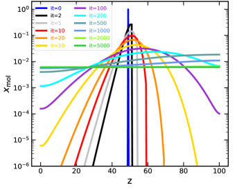
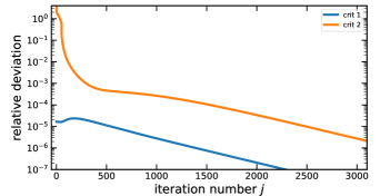
Figure 13: Test of the iterative numerical method to solve the diffusion equation without chemical sources and sinks. We consider a $\delta$-peak for the initial concentration $x_{\rm mol}=n_{i,k}/n_{k}$ at the start of the iterations in a Gaussian density structure, see text. The upper figure shows the concentrations as function of the number of iterations carried out. The lower figure shows the relative deviations between iterations, see Eqs. (27) and (28).

A.3 Initial condition

The very first disc iteration is computed with zero mixing rates. In all forthcoming iterations, the mixing rates are activated.

A.4 Test of the numerical solution method

To verify our numerical implementation, we made a quick test to check the capabilities of our simple iterative scheme. We considered a Gaussian density profile on an equidistant spatial grid with 101 points $k\!=\!1...101$

$$z_{k}= \leavevmode\nobreak\ k-1$$ (42)

$$n_{k}= \leavevmode\nobreak\ \exp\Big{(}-\Big{(}\frac{z_{k}}{20}\Big{)}^{2}\Big{)}$$ (43)

$$K_{k}= \leavevmode\nobreak\ 1$$ (44)

$$D_{i,k}= \leavevmode\nobreak\ 0$$ (45)

and choose, for a single test species $i\!=\!1$, the following initial condition

$$n_{i,k}=\left\{\begin{array}[]{ll}1&,\ k=50\\ 0&,\ \mbox{otherwise}\end{array}\right.$$ (46)

at the start of the iteration. Then we copied the exact implementation of the vertical mixing in ProDiMo to an external tool where we omit the chemical source and sink terms $P_{i,k}$ and $L_{i,k}$. In a loop from $k\!=\!K$ down to 1, we then

• calculate ${\cal A}_{i,k}$, ${\cal B}_{i,k}$ and ${\cal C}_{i,k}$, and
  

• solve the rate equation without chemical sources and sinks $n_{i,k}=\frac{1}{{\cal B}_{i,k}}\left({\cal A}_{i,k}\,n_{i,k+1}+{\cal C}_{i,k}\,n_{i,k-1}\right)$.

This numerical scheme mimics the downward sweep in ProDiMo while solving the chemistry in the time-independent case from top to bottom. Figure 13 shows the resulting concentrations $n_{i,k}/n_{k}$ as function of $z$, where $z\!=\!0$ represents the midplane. The results after selected numbers of iterations are plotted with different colours as indicated. This plot can be compared to our results with chemical sources and sinks plotted in Fig. 2 in the main part of the paper.

The figure indicates that up to 5000 iterations are required to reach a constant concentration as physically expected in this setup. The final value of that constant concentration results to be 0.61%, which is close to the predicted value of 0.63% that we get from a numerical integral of $n_{ik}(z)$ over $z$ in the initial state, divided by the numerical integral of $n(z)$. We note that in real applications that include the chemical source terms, the chemicals will rarely travel many scale heights. Instead, there are normally some dominant, but spatially restricted formation and destruction regions, and the model must properly describe the diffusive transport between those regions, hence we expect a couple of hundred iterations to be sufficient.

Figure 13 demonstrates the numerical behaviour during the course of the iterations:

• The first few tens of iterations are featured by an asymmetry, because the resultant $n_{i,k+1}$ is used already for the determination of $n_{i,k}$ whereas $n_{i,k-1}$ is not. Therefore, the information of a certain molecule being mixed downward is travelling faster downwards than it travels upwards.

• After some hundreds of iterations, however, the upper regions fill in quicker than the lower regions. This is because of the density gradient in the system, i.e. a large reservoir in the denser lower disc regions is able to more quickly fill in the low-density regions above than vice versa.