Asymptotic Theory for Regularized System Identification Part I: Empirical Bayes Hyper-parameter Estimator

Abstract

Regularized techniques, also named as kernel-based techniques, are the major advances in system identification in the last decade. Although many promising results have been achieved, their theoretical analysis is far from complete and there are still many key problems to be solved. One of them is the asymptotic theory, which is about convergence properties of the model estimators as the sample size goes to infinity. The existing related results for regularized system identification are about the almost sure convergence of various hyper-parameter estimators. A common problem of those results is that they do not contain information on the factors that affect the convergence properties of those hyper-parameter estimators, e.g., the regression matrix. In this paper, we tackle problems of this kind for the regularized finite impulse response model estimation with the empirical Bayes (EB) hyper-parameter estimator and filtered white noise input. In order to expose and find those factors, we study the convergence in distribution of the EB hyper-parameter estimator, and the asymptotic distribution of its corresponding model estimator. For illustration, we run Monte Carlo simulations to show the efficacy of our obtained theoretical results.

Asymptotic theory, Empirical Bayes, Hyper-parameter estimator, Regularized least squares, Asymptotic distribution, Ridge regression.

1 Introduction

In the last decade, there has been a surge of interests to study linear time-invariant (LTI) system identification problems by estimating impulse response models of LTI systems with regularized least squares (RLS) methods, and this research direction is often called regularized system identification. Many results have been reported in this direction, addressing, e.g., the regularization design and analysis [2, 18, 1, 33, 30], and the efficient implementations [5, 3]; for more references, the interested readers are referred to the survey/tutorial papers [26, 7, 17] and the book [23]. These results make the regularized system identification become not only a complement to classic system identification based on the maximum likelihood/prediction error methods (ML/PEM) and its asymptotic theory [16], but also an emerging new system identification paradigm [17]. The success of RLS is due to at least the following three factors. First, the underlying model structure is determined by a carefully designed regularization term that incorporates the prior knowledge of the system to be identified, such as stability and dominant dynamics, thus enhancing the estimation performance. Second, model complexity is governed by a continuous hyper-parameter used to parametrize the regularization term, which can be tuned more flexibly w.r.t. discrete orders used in classic system identification. Third, the connections of RLS with kernel methods [8] and Bayesian methods [27] enable the usage of ideas and tools from the latter, which enriches our ideas and tools, and enhances our capability in dealing with system identification problems.

Although many promising results have been achieved, there are still many key problems to be solved. One of them is the asymptotic theory, which is the theory of convergence properties of the model estimators as the sample size goes to infinity and that is widely used to assess the quality of model estimators. For classic system identification, asymptotic theory has been widely studied [16]. However, for regularized system identification, the study of the asymptotic theory just started and only very few results have been reported so far [24, 21, 20, 11, 12]. In particular, the almost sure convergence of the empirical Bayes ($\operatorname*{EB}$) hyper-parameter estimator has been studied in [24] and [21] for scalably and generally parameterized regularization term, respectively. In [21, 20], we studied the almost sure convergence of the Stein’s unbiased risk estimator (SURE) and the generalized cross validation ($\operatorname*{GCV}$) hyper-parameter estimators, and showed that they are both asymptotically optimal in the sense of minimizing the mean square error (MSE). In [11, 12], one asymptotic approximation of MSE is studied. A common problem of these results is that they do not contain information on the factors that affect the convergence properties of the hyper-parameter estimators. For example, it has been shown in [21] that the EB hyper-parameter estimator converges to its limit with a rate of $1/\sqrt{N}$, where $N$ is the sample size, but this information is rough. In fact, it is well known from numerical simulations, e.g., [26, 21], that the more ill-conditioned the regression matrix, the more samples needed to get an RLS estimator with good quality. A conjecture is that the more ill-conditioned the regression matrix, the more slowly the EB hyper-parameter estimator converges to its limit, but there have been no theoretical results to support this conjecture so far.

In this paper, we tackle problems of this kind and try to build up the asymptotic theory for the regularized system identification based on some fundamental results in [14]. In particular, we consider the regularized finite impulse response (FIR) model estimation with the EB hyper-parameter estimator and filtered white noise input. In order to expose and find the factors that affect the convergence properties of the EB hyper-parameter estimator and the corresponding RLS estimator, we first study the convergence in distribution of the EB hyper-parameter estimator and then the asymptotic distribution of the RLS estimator. Moreover, we make the analysis in the following order: first generally parameterized regularization, and then the ridge regression [10] as an illustration. Finally, we run Monte Carlo simulations to show the efficacy of our theoretical results.

The remaining parts of this paper are organized as follows. In Section 2, we first introduce some preliminary materials and then the problem statement. We then study in Section 3 the convergence in distribution of the EB hyper-parameter estimator to its limit, and in Section 4, the asymptotic distribution of the corresponding RLS estimator to the true model parameter. In Section 5, we consider the ridge regression with filtered white noise inputs as an illustration. In Section 6, we run Monte Carlo simulations to demonstrate our theoretical results. All proofs of theorems and propositions are included in Appendix A.

2 Preliminary and Problem Statement

In this section, we first introduce some preliminary background materials and then the problem statement of this paper.

2.1 FIR Model Estimation

We focus on the finite impulse response (FIR) model

$$y(t)=\sum_{i=1}^{n}g_{i}u(t-i)+v(t),\ t=1,\cdots,N,$$ (1)

where $n$ is the order of FIR model, $t\in\mathbb{N}$ is the time index, $N$ is the sample size and usually assumed to be larger than $n$, $u(t)\in{\mathbb{R}}$, $y(t)\in{\mathbb{R}}$, and $v(t)\in{\mathbb{R}}$ are the input, output and measurement noise at time $t$, respectively, and $g_{1},\cdots,g_{n}\in{\mathbb{R}}$ are FIR model parameters to be estimated.

Model (1) can be rewritten in a vector-matrix format:

$$Y=\Phi\theta+V,$$ (2)

where

$$Y= \left[\begin{array}[]{cccc}y(1)&y(2)&\cdots&y(N)\end{array}\right]^{T},$$ (3b)

$$\Phi= \left[\begin{array}[]{cccc}\phi(1)&\phi(2)&\cdots&\phi(N)\end{array}\right]^{T},$$ (3d)

$$\theta= \left[\begin{array}[]{cccc}g_{1}&g_{2}&\cdots&g_{n}\end{array}\right]^{T},$$ (3f)

$$V= \left[\begin{array}[]{cccc}v(1)&v(2)&\cdots&v(N)\end{array}\right]^{T}$$ (3h)

with $\phi(t)=\left[\begin{array}[]{cccc}u(t-1)&u(t-2)&\cdots&u(t-n)\end{array}\right]^{T}$ and $u(t)=0$ for $t<0$. Here, $\Phi$ is often known as the regression matrix. The FIR model estimation is to estimate the unknown $\theta$ as “well” as possible based on data $\{y(t),\phi(t)\}_{t=1}^{N}$.

The theoretical analysis of the FIR model estimation is often done in a probabilistic framework. To this goal, we first make assumptions on the input $u(t)$ and the measurement noise $v(t)$.

Assumption 1

The input $u(t)$ with $t=1-n,\cdots,N-1$ is white noise filtered with the stable filter $H(q)$, i.e.,

$$H(q)= \sum_{k=0}^{\infty}h(k)q^{-k}\ \text{with}\ \sum_{k=0}^{\infty}|h(k)|<\infty,$$ (4a)

$$u(t)= H(q)e(t)=\sum_{k=0}^{\infty}h(k)e(t-k),$$ (4b)

where $q^{-1}$ represents the backward shift operator, i.e., $q^{-1}u(t)=u(t-1)$, and $e(t)$ is independent and identically distributed ($i.i.d.$) with zero mean, variance $\sigma_{e}^{2}>0$, bounded moments of order $4+\delta$ for some $\delta>0$, and ${\mathbb{E}}[e(t)^{4}]=c\sigma_{e}^{4}$ with a constant $c>0$. Moreover, we let

$$\Sigma={\mathbb{C}\mathbb{O}\mathbb{V}}(\left[\begin{array}[]{cccc}u(0)&u(1)&\cdots&u(n-1)\end{array}\right]^{T}),$$ (6)

where ${\mathbb{C}\mathbb{O}\mathbb{V}}(\cdot)$ denotes the covariance matrix, and assume that $\Sigma$ is positive definite, i.e. $\Sigma\succ 0$.

Assumption 2

The measurement noise $v(t)$ is $i.i.d.$ with zero mean, variance $\sigma^{2}>0$, and bounded moments of order $4+\delta$ for some $\delta>0$.

Assumption 3

$\{e(t)\}_{t=-\infty}^{N-1}$ and $\{v(t)\}_{t=1}^{N}$ are mutually independent, which means that for $i=-\infty,\cdots,N-1$ and $j=1,\cdots,N$, $e(i)$ and $v(j)$ are independent.

Remark 1

By Assumptions 1 and 3, it is easy to verify that $u(t)$ is a stationary stochastic process, independent of $v(t)$, with

$${\mathbb{E}}[u(t)] =0,$$ (7a)

$${\mathbb{E}}[u(t)u(t+\tau)] \triangleq R_{u}(\tau)=\sigma_{e}^{2}\sum_{k=0}^{\infty}h(k)h(k+\tau),$$ (7b)

where ${\mathbb{E}}(\cdot)$ denotes the mathematical expectation, $\tau\geq 0$, and $R_{u}(\tau)=R_{u}(-\tau)$. Moreover, the $(i,j)$th element of $\Sigma$ in (6) is $R_{u}(|i-j|)$, which is determined by the filter $H(q)$ and often has no closed-form expression.

Assumption 4

The regression matrix $\Phi\in{\mathbb{R}}^{N\times n}$ with $N>n$ has full column rank, i.e. $\operatorname*{rank}(\Phi)=n$.

We use the mean square error (MSE) in relation to the impulse response estimation to assess how “good” an estimator $\hat{\theta}\in{\mathbb{R}}^{n}$ of the true parameter $\theta_{0}=\left[\begin{array}[]{cccc}g_{1}^{0}&g_{2}^{0}&\cdots&g_{n}^{0}\end{array}\right]^{T}\in{\mathbb{R}}^{n}$ is [6, 24]. The MSE is defined as follows,

$${\operatorname*{MSE}}_{g}(\hat{\theta})= {\mathbb{E}}(\|\hat{\theta}-\theta_{0}\|_{2}^{2}),$$ (8)

where $\|\cdot\|_{2}$ denotes the Euclidean norm. The smaller MSE indicates the better quality of $\hat{\theta}$.

Remark 2

We make the assumption that the dimension $n$ should be large enough to capture the dynamics of the underlying system to be identified. This is made possible, because the model complexity of the regularized FIR model estimator is governed by the hyper-parameter and tuned in a continuous way (see, e.g., [23]).

2.2 The Least Squares Method

Under Assumption 4, the simplest method for FIR model estimation is the Least Squares (LS):

$$\hat{\theta}^{\operatorname*{LS}}= \operatorname*{arg\,min}_{\theta\in{\mathbb{R}}^{n}}\|Y-\Phi\theta\|_{2}^{2}$$ (9a)

$$= (\Phi^{T}\Phi)^{-1}\Phi^{T}Y.$$ (9b)

Recall the convergence in distribution in statistics and let

$$V_{1}^{\operatorname*{ALS}}= \sigma^{2}\Sigma^{-1}.$$ (10)

Then it is well known that

$$\sqrt{N}(\hat{\theta}^{\operatorname*{LS}}-\theta_{0})\overset{d.}{\to} \mathcal{N}(0,V^{\operatorname*{ALS}}_{1}),$$ (11)

which indicates that if $\Sigma$ is ill-conditioned, then $\sqrt{N}(\hat{\theta}^{\operatorname*{LS}}-\theta_{0})$ may have large limiting variance.

2.3 The Regularized Least Squares Method

To handle the ill-conditioned problem, one can introduce a regularization term in (9a) to obtain the regularized least squares (RLS) estimator:

$$\hat{\theta}^{\operatorname*{R}}= \operatorname*{arg\,min}_{\theta\in{\mathbb{R}}^{n}}\|Y-\Phi\theta\|_{2}^{2}+\sigma^{2}\theta^{T}P^{-1}\theta$$ (12a)

$$= (\Phi^{T}\Phi+\sigma^{2}P^{-1})^{-1}\Phi^{T}Y$$ (12b)

$$= P\Phi^{T}Q^{-1}Y,$$ (12c)

where $P\in{\mathbb{R}}^{n\times n}$ is positive semidefinite, its $(i,j)$th element $[P]_{i,j}$ can be designed through a positive semidefinite kernel $\kappa(i,j;\eta):\mathbb{N}\times\mathbb{N}\to{\mathbb{R}}$, thus, $P$ is often called the kernel matrix with $\eta\in\Omega\subset{\mathbb{R}}^{p}$ being the hyper-parameter, and

$$Q=\Phi P\Phi^{T}+\sigma^{2}I_{N},$$ (13)

and $I_{N}$ denotes the $N$-dimensional identity matrix.

There are two key issues for the RLS method: the kernel design and the hyper-parameter estimation.

2.3.1 Kernel Design

The goal of kernel design is to embed the prior knowledge of the system to be identified in the kernel $\kappa(i,j;\eta)$ by parameterization of the kernel with the hyper-parameter $\eta$.

The mostly widely used kernels include

$$\text{SS}: \kappa(i,j;\eta)=c\left(\frac{\alpha^{i+j+\max(i,j)}}{2}-\frac{\alpha^{3\max(i,j)}}{6}\right)$$

$$\eta=[c,\alpha]\in\Omega=\{c\geq 0,\ \alpha\in[0,1)\},$$ (14a)

$$\text{DC}: \kappa(i,j;\eta)=c\alpha^{(i+j)/2}\rho^{|i-j|},$$

$$\eta=[c,\alpha,\rho]\in\Omega=\{c\geq 0,\ \alpha\in[0,1),\ |\rho|\leq 1\},$$ (14b)

$$\text{TC}: \kappa(i,j;\eta)=c\alpha^{\max(i,j)},$$

$$\eta=[c,\alpha]\in\Omega=\{c\geq 0,\ \alpha\in[0,1)\},$$ (14c)

where the stable spline (SS) kernel (14) is introduced in [25], the diagonal correlated (DC) kernel (14) and the tuned-correlated (TC) kernel (14) (also named as the first order stable spline kernel) are introduced in [6].

2.3.2 Hyper-parameter Estimation

Given a designed kernel, the next step is to estimate the hyper-parameter $\eta$. There are many methods, such as the empirical Bayes (EB), Stein’s unbiased risk estimation (SURE) and generalized cross validation (GCV) method (see, e.g., [26]).

In the sequel, we consider the $\operatorname*{EB}$ method, which assumes that $\theta$ and $V$ are independent and Gaussian distributed, i.e.,

$$\theta\sim\mathcal{N}({0},P),\ V\sim\mathcal{N}({0},\sigma^{2}I_{N}),$$ (15)

$$\Rightarrow Y\sim\mathcal{N}({0},\Phi P\Phi^{T}+\sigma^{2}I_{N}).$$ (16)

Then, hyper-parameters are found by maximizing the marginal likelihood function of $Y$ given $\eta$, which is equivalent to minimizing

$$\mathscr{F}_{\operatorname*{EB}}= Y^{T}Q^{-1}Y+\log\det(Q),$$ (17)

where $\det(\cdot)$ denotes the determinant of a square matrix and $Q$ is defined as in (13). Moreover, as the noise variance is unknown in practice, we use an unbiased estimator of $\sigma^{2}$,

$$\widehat{\sigma^{2}}= \frac{\|Y-\Phi\hat{\theta}^{\operatorname*{LS}}\|_{2}^{2}}{N-n}=\frac{Y^{T}\left[I_{N}-\Phi(\Phi^{T}\Phi)^{-1}\Phi^{T}\right]Y}{N-n}.$$ (18)

Remark 3

As mentioned in [26, Remark 5], one alternative way to estimate the unknown $\sigma^{2}$ is to consider it as an additional “hyper-parameter” included in $\eta$. In such case, the convergence properties of the corresponding hyper-parameter estimator and RLS estimator will be different from those shown in this paper, which will be shown in another paper of this series of papers.

Replacing $\sigma^{2}$ with $\widehat{\sigma^{2}}$, the $\operatorname*{EB}$ hyper-parameter estimator can be represented as

$$\text{EB}:\hat{\eta}_{\text{EB}}= \operatorname*{arg\,min}_{\eta\in\Omega}\widehat{\mathscr{F}_{\operatorname*{EB}}}(\eta)$$ (19a)

$$\widehat{\mathscr{F}_{\operatorname*{EB}}}(\eta)= Y^{T}\hat{Q}(\eta)^{-1}Y+\log\det(\hat{Q}(\eta)),$$ (19b)

where

$$\hat{Q}(\eta)=\Phi P(\eta)\Phi^{T}+\widehat{\sigma^{2}}I_{N}.$$ (20)

With (19a) and $\widehat{\sigma^{2}}$, the RLS estimator (12) becomes

$$\hat{\theta}^{\operatorname*{R}}(\hat{\eta}_{\text{EB}})=P(\hat{\eta}_{\text{EB}})\Phi^{T}\hat{Q}(\hat{\eta}_{\text{EB}})^{-1}Y.$$ (21)

2.4 Problem Statement

In this paper, we study the convergence properties of the EB hyper-parameter estimator $\hat{\eta}_{\text{EB}}$ in (19a) and the corresponding RLS estimator $\hat{\theta}^{\operatorname*{R}}(\hat{\eta}_{\text{EB}})$ in (21) as the sample size $N$ goes to infinity. In fact, we have studied in [21] the almost sure convergence of $\hat{\eta}_{\text{EB}}$, and then we realized that it does not contain information on the factors that affect the convergence properties of $\hat{\eta}_{\text{EB}}$. To be more specific, we briefly recall the convergence result of $\hat{\eta}_{\text{EB}}$ in [21]. To state the result, we make the following assumptions, which are also needed in this paper.

Assumption 5

The hyper-parameter estimator $\hat{\eta}_{\text{EB}}$ is an interior point of $\Omega$ and $\Omega$ is a compact set, where $\Omega$ is irrespective of $N$.

Remark 4

Assumption 5 is common in both classical system identification, e.g., [16], and the regularized system identification, e.g., [21, 24]. However, it must be stressed that the proposed analysis of this paper is thus subject to some limitations. In particular, the proposed analysis cannot be applied to problems where $\hat{\eta}_{\operatorname*{EB}}$ lies on the boundary, e.g., the network identification problems in [32, 31] and the sparse Bayesian learning and its application in [29, 4].

Assumption 6

$P(\eta)$ is positive definite, continuously differentiable, and twice continuously differentiable at every $\eta\in\Omega$.

Assumption 7

The set $\eta_{\operatorname*{b}}^{*}$, defined as

$$\eta_{\operatorname*{b}}^{*}= \operatorname*{arg\,min}_{\eta\in\Omega}W_{\operatorname*{b}}(P,\theta_{0})$$ (22a)

$$W_{\operatorname*{b}}(P,\theta_{0})= \theta_{0}^{T}P^{-1}\theta_{0}+\log\det(P),$$ (22b)

contains interior points of $\Omega$ and is made of isolated points.

Then by Assumptions 2 and 4-7, when we considered the deterministic inputs satisfying $\lim_{N\to\infty}\Phi^{T}\Phi/N=\Sigma$ and used the true noise variance $\sigma^{2}$, it was shown in [21, Theorems 1 and 2]

1. the almost sure convergence of $\hat{\eta}_{\operatorname*{EB}}$, i.e.,

   $$\hat{\eta}_{\operatorname*{EB}}\overset{a.s.}{\to} \eta_{\operatorname*{b}}^{*};$$ (23)

2. how fast the convergence of $\hat{\eta}_{\operatorname*{EB}}$ to $\eta_{\operatorname*{b}}^{*}$ only depends on $\|\hat{\theta}^{\operatorname*{LS}}-\theta_{0}\|_{2}=O_{p}(1/\sqrt{N})$, as shown in [14, Theorem 3], and is at a rate of $1/\sqrt{N}$, i.e.,

   $$\|\hat{\eta}_{\operatorname*{EB}}-\eta_{\operatorname*{b}}^{*}\|_{2}=O_{p}(1/\sqrt{N}).$$ (24)

   For convenience, this rate is called the “convergence rate” of $\hat{\eta}_{\operatorname*{EB}}$ to $\eta_{\operatorname*{b}}^{*}$ in the sequel.

Now it is clear to see that (23) and (24) do not contain any information on the factors that affect the convergence properties of $\hat{\eta}_{\text{EB}}$ to $\eta_{\operatorname*{b}}^{*}$, e.g., the regression matrix $\Phi$ and the kernel matrix $P$. It must be stressed that to know such information has both theoretical and practical significance. For instance, it is well known from numerical simulations (see, e.g., [26, 21]) that when the filter $H(q)$ in (4) is low-pass ($\Phi$ is thus ill-conditioned), it takes more samples to obtain $\hat{\theta}^{\operatorname*{R}}(\hat{\eta}_{\text{EB}})$ with good quality. A conjecture is that the more ill-conditioned $\Phi$, the more slowly $\hat{\eta}_{\text{EB}}$ converges to $\eta_{\operatorname*{b}}^{*}$. However, there have been no theoretical results to support this so far. In this paper, we try to tackle problems of this kind and in particular, we study how to expose and find the factors that affect the convergence properties of $\hat{\eta}_{\text{EB}}$ to $\eta_{\operatorname*{b}}^{*}$, and $\hat{\theta}^{\operatorname*{R}}(\hat{\eta}_{\text{EB}})$ to $\theta_{0}$. It is also well known from numerical simulations (see, e.g., [26, 21]) that, $\hat{\theta}^{\operatorname*{R}}(\hat{\eta}_{\text{EB}})$ and $\hat{\theta}^{\operatorname*{LS}}$ may behave quite differently, especially when $\Phi$ is ill-conditioned. However, when checking the asymptotic properties of $\hat{\theta}^{\operatorname*{R}}(\hat{\eta}_{\text{EB}})$ and $\hat{\theta}^{\operatorname*{LS}}$, and in particular, the frequently used almost sure convergence and convergence in distribution, we find that they have the same convergence properties. This finding gives us the intuition to consider instead the high order asymptotic distribution to explain the different behaviors between $\hat{\theta}^{\operatorname*{R}}(\hat{\eta}_{\text{EB}})$ and $\hat{\theta}^{\operatorname*{LS}}$.

2.5 Some Preliminary Results

Before proceeding to the discussions of the convergence properties of $\hat{\eta}_{\operatorname*{EB}}$ in (19a) and $\hat{\theta}^{\operatorname*{R}}(\hat{\eta}_{\operatorname*{EB}})$ in (21), we first state the following lemma, whose proof can be found in [14].

Lemma 1

For the FIR model (1) mentioned in Section 2, under Assumptions 1-3, if $P(\eta)$ is differentiable for every $\eta\in\Omega$, we have the following results.

1. As mentioned in [14, Theorems 1-2], we have

   $$N(\Phi^{T}\Phi)^{-1}\overset{a.s.}{\to}\Sigma^{-1},$$ (25)

   $$\frac{\Phi^{T}V}{N}\overset{a.s.}{\to}0,$$ (26)

   $$\widehat{\sigma^{2}}\overset{a.s.}{\to}\sigma^{2},$$ (27)

   $$\left(\sqrt{N}\left(N(\Phi^{T}\Phi)^{-1}-\Sigma^{-1}\right),\sqrt{N}\Phi^{T}V/N,\sqrt{N}(\widehat{\sigma^{2}}-\sigma^{2})\right)$$

   $$\overset{d.}{\to}\left(-\Sigma^{-1}\Gamma\Sigma^{-1},\upsilon,\rho\right),$$ (28)

   where $\Gamma\in{\mathbb{R}}^{n\times n}$, $\upsilon\in{\mathbb{R}}^{n}$ and $\rho\in{\mathbb{R}}$ are jointly Gaussian distributed with

   $${\mathbb{E}}(\Gamma)=0,{\mathbb{E}}(\upsilon)=0,{\mathbb{E}}(\rho)=0,$$ (29a)

   $${C_{\Gamma}={\mathbb{E}}(\Gamma\otimes\Gamma),}$$

   $${\ \quad=\lim_{N\to\infty}N{\mathbb{E}}\left[\left(\frac{\Phi^{T}\Phi}{N}-\Sigma\right)\otimes\left(\frac{\Phi^{T}\Phi}{N}-\Sigma\right)\right],}$$ (29b)

   $${\mathbb{E}}(\upsilon\upsilon^{T})=\sigma^{2}\Sigma,{\mathbb{E}}(\rho^{2})={\mathbb{E}}[(v(t))^{4}]-\sigma^{4},$$ (29c)

   $${\mathbb{E}}(\upsilon\otimes\Gamma)=0,{\mathbb{E}}(\rho\upsilon)=0,{\mathbb{E}}(\rho\Gamma)=0,$$ (29d)

   and $\otimes$ denotes the Kronecker product. Moreover, for $i,j=1,\cdots,n$, the $(i,j)$th element of $\Sigma$ can be represented as $\left[\Sigma\right]_{i,j}=R_{u}(|i-j|);$ for $i,j=1,\cdots,n^{2}$, the $(i,j)$th element of $C_{\Gamma}$ is

   $$[C_{\Gamma}]_{i,j}=\left\{{\mathbb{E}}[e(t)]^{4}/\sigma_{e}^{4}-3\right\}R_{u}(k)R_{u}(l)$$ (30)

   $$+\sum_{\tau=-\infty}^{\infty}\left[R_{u}(\tau)R_{u}(\tau+k-l)+R_{u}(\tau+k)R_{u}(\tau-l)\right],$$

   where $R_{u}(\tau)$ is defined in (7b),

   $$k= \left|\lfloor{(i-1)/n}\rfloor-\lfloor{(j-1)/n}\rfloor\right|,$$ (31a)

   $$l= |i-j-\lfloor{(i-1)/n}\rfloor n+\lfloor{(j-1)/n}\rfloor n|,$$ (31b)

   $|\cdot|$ denotes the absolute value, and $\lfloor{\cdot}\rfloor$ denotes the floor operation, i.e. $\lfloor{x}\rfloor=\max\{\tilde{x}\in{\mathbb{Z}}|\tilde{x}\leq x\}$.

2. As mentioned in [14, Theorem 7, (44)-(47)], for any given $\eta\in{\mathbb{R}}^{p}$ and

   $${\hat{S}(\eta)=P({\eta})+\widehat{\sigma^{2}}(\Phi^{T}\Phi)^{-1},}$$ (32)

   it holds that

   $$\hat{S}(\eta)^{-1}\overset{a.s.}{\to}P(\eta)^{-1},$$ (33)

   $$\sqrt{N}(\hat{S}(\eta)^{-1}-P(\eta)^{-1})\overset{a.s.}{\to}0,$$ (34)

   $$\frac{\partial\hat{S}(\eta)^{-1}}{\partial\eta_{k}}\overset{a.s.}{\to}\frac{\partial P(\eta)^{-1}}{\partial\eta_{k}},$$ (35)

   $$\sqrt{N}\left(\frac{\partial\hat{S}(\eta)^{-1}}{\partial\eta_{k}}-\frac{\partial P(\eta)^{-1}}{\partial\eta_{k}}\right)\overset{a.s.}{\to}0,$$ (36)

   where $\eta_{k}$ denotes the $k$th element of $\eta$ and $k=1,\cdots,p$.

3. As mentioned in [14, Theorem 7, (49)], for any estimator $\hat{\eta}_{N}\in{\mathbb{R}}^{p}$ of $\eta\in{\mathbb{R}}^{p}$ with $\hat{\eta}_{N}\overset{a.s.}{\to}\eta^{*}\in{\mathbb{R}}^{p}$, it holds that

   $$\hat{S}(\hat{\eta}_{N})^{-1}-P(\eta^{*})^{-1}$$

   $$= -\hat{S}(\hat{\eta}_{N})^{-1}\left[\sum_{k=1}^{p}\left.\frac{\partial P(\eta)}{\partial\eta_{k}}\right|_{\eta=\tilde{\eta}_{N}}e_{k}^{T}(\hat{\eta}_{N}-\eta^{*})\right]P(\eta^{*})^{-1}$$

   $$-\widehat{\sigma^{2}}\hat{S}(\hat{\eta}_{N})^{-1}(\Phi^{T}\Phi)^{-1}P(\eta^{*})^{-1},$$ (37)

   where $e_{k}\in{\mathbb{R}}^{p}$ denotes a column vector with $k$th element being one and others zero, and $\tilde{\eta}_{N}$ belongs to a neighborhood of $\eta^{*}$ with radius $\|\hat{\eta}_{N}-\eta^{*}\|_{2}$.

4. As mentioned in [14, Theorem 7, (51)], for any given $\eta\in{\mathbb{R}}^{p}$, it holds that

   $$\hat{S}(\eta)^{-1}-P(\eta)^{-1}=-\frac{1}{N}\widehat{\sigma^{2}}\hat{S}(\eta)^{-1}N(\Phi^{T}\Phi)^{-1}P(\eta)^{-1}.$$ (38)

3 Convergence in Distribution of the $\operatorname*{EB}$ Hyper-parameter Estimator

To expose the factors that affect the convergence properties of $\hat{\eta}_{\text{EB}}$ to $\eta_{\operatorname*{b}}^{*}$, we study the convergence in distribution of $\sqrt{N}(\hat{\eta}_{\operatorname*{EB}}-\eta_{\operatorname*{b}}^{*})$ under the following additional assumptions.

Assumption 8

$\eta_{\operatorname*{b}}^{*}$ consists of only one point.

Remark 5

Assumption 8 is common in the analysis of convergence in distribution of model estimators, (see, e.g., [16, Theorem 9.1]).

Assumption 9

The first-order derivative of $P(\eta)$ with respect to $\eta$ at $\eta=\eta_{\operatorname*{b}}^{*}$ is nonzero, i.e. at least one of $k=1,\cdots,p$, $\left.{\partial P(\eta)}/{\partial\eta_{k}}\right|_{\eta=\eta_{\operatorname*{b}}^{*}}\not=0$.

Remark 6

If for all $k=1,\cdots,p$, $\left.{\partial P(\eta)}/{\partial\eta_{k}}\right|_{\eta=\eta_{\operatorname*{b}}^{*}}=0$, then $A_{\operatorname*{b}}(\eta^{*}_{\operatorname*{b}})$ in (1) and $B_{\operatorname*{b}}(\eta^{*}_{\operatorname*{b}})$ in (42) will be zero matrices, leading to the meaningless convergence in distribution results in the following theorem.

Theorem 1

Under Assumptions 1-7, (23) holds true. Moreover, under additional Assumptions 8-9, we have

$$\sqrt{N}(\hat{\eta}_{\operatorname*{EB}}-\eta^{*}_{\operatorname*{b}})\overset{d.}{\to}\mathcal{N}(0,V_{\operatorname*{b}}^{\operatorname*{H}}(\eta_{\operatorname*{b}}^{*})),$$ (39)

$$V_{\operatorname*{b}}^{\operatorname*{H}}(\eta_{\operatorname*{b}}^{*})=4\sigma^{2}A_{\operatorname*{b}}(\eta^{*}_{\operatorname*{b}})^{-1}B_{\operatorname*{b}}(\eta^{*}_{\operatorname*{b}})\Sigma^{-1}B_{\operatorname*{b}}(\eta^{*}_{\operatorname*{b}})^{T}A_{\operatorname*{b}}(\eta^{*}_{\operatorname*{b}})^{-1},$$ (40)

where for $k,l=1,\cdots,p$, the $(k,l)$th element of $A_{\operatorname*{b}}(\eta^{*}_{\operatorname*{b}})\in{\mathbb{R}}^{p\times p}$ can be represented as

$$\left[A_{\operatorname*{b}}(\eta^{*}_{\operatorname*{b}})\right]_{k,l}= \left\{\theta_{0}^{T}\frac{\partial^{2}P^{-1}}{\partial\eta_{k}\partial\eta_{l}}\theta_{0}+{\operatorname*{Tr}}\left(\frac{\partial P^{-1}}{\partial\eta_{l}}\frac{\partial P}{\partial\eta_{k}}\right)\right.$$

$$+\left.\left.\operatorname*{Tr}\left(P^{-1}\frac{\partial^{2}P}{\partial\eta_{k}\partial\eta_{l}}\right)\right\}\right|_{\eta=\eta^{*}_{\operatorname*{b}}},$$ (41)

the $k$th row of $B_{\operatorname*{b}}(\eta^{*}_{\operatorname*{b}})\in{\mathbb{R}}^{p\times n}$ can be represented as

$$\left[B_{\operatorname*{b}}(\eta^{*}_{\operatorname*{b}})\right]_{k,:}= \theta_{0}^{T}\left.\frac{\partial P^{-1}}{\partial\eta_{k}}\right|_{\eta=\eta_{\operatorname*{b}}^{*}}.$$ (42)

Remark 7

If we consider deterministic inputs and assume that $\lim_{N\to\infty}\Phi^{T}\Phi/N=\Sigma$, Theorem 1 still holds.

Clearly, Theorem 1 shows that the limiting covariance matrix $V_{\operatorname*{b}}^{\operatorname*{H}}(\eta_{\operatorname*{b}}^{*})$ contains the factors that affect the convergence properties of $\hat{\eta}_{\operatorname*{EB}}$ to $\eta_{\operatorname*{b}}^{*}$, including the limit of $\Phi^{T}\Phi/N$, i.e., $\Sigma$, the kernel matrix $P$, and the true value of $\theta$, i.e., $\theta_{0}$. Moreover, the following proposition shows that as the condition number of $\Sigma$ increases, $\operatorname*{Tr}[V_{\operatorname*{b}}^{\operatorname*{H}}(\eta_{\operatorname*{b}}^{*})]$ becomes or tends to become larger, indicating that the more slowly $\hat{\eta}_{\operatorname*{EB}}$ converges to $\eta_{\operatorname*{b}}^{*}$.

Proposition 1

Define the eigenvalue decomposition (EVD) of $\Sigma$ as follows,

$$\Sigma= \sum_{i=1}^{n}\lambda_{i}(\Sigma)e_{\Sigma,i}e_{\Sigma,i}^{T},$$ (43)

where $\lambda_{1}(\Sigma)\geq\cdots\geq\lambda_{n}(\Sigma)>0$ denote eigenvalues of $\Sigma$ and $e_{\Sigma,i}\in{\mathbb{R}}^{n}$ denotes the eigenvector of $\Sigma$ associated with $\lambda_{i}(\Sigma)$; moreover, the condition number of $\Sigma$ is defined as $\operatorname*{cond}(\Sigma)=\lambda_{1}(\Sigma)/\lambda_{n}(\Sigma)$. If $\sigma^{2}$, $\theta_{0}$, $P$, $e_{\Sigma,1},\cdots,e_{\Sigma,n}$ and $\lambda_{1}(\Sigma),\cdots,\lambda_{n-1}(\Sigma)$ are fixed, as $\lambda_{n}(\Sigma)$ decreases ($\operatorname*{cond}(\Sigma)$ increases), $\operatorname*{Tr}[V_{\operatorname*{b}}^{\operatorname*{H}}(\eta_{\operatorname*{b}}^{*})]$ will increase. More generally, if

$$e_{\Sigma,n}^{T}B_{\operatorname*{b}}(\eta_{\operatorname*{b}}^{*})^{T}A_{\operatorname*{b}}(\eta_{\operatorname*{b}}^{*})^{-1}\not=0,$$ (44)

there exist $B_{L}^{\operatorname*{b}},B_{U}^{\operatorname*{b}}>0$, irrespective of $\operatorname*{cond}(\Sigma)$, such that

$$\frac{B_{L}^{\operatorname*{b}}}{\lambda_{1}(\Sigma)}\operatorname*{cond}(\Sigma)\leq\operatorname*{Tr}[V_{\operatorname*{b}}^{\operatorname*{H}}(\eta_{\operatorname*{b}}^{*})]\leq\frac{B_{U}^{\operatorname*{b}}}{\lambda_{1}(\Sigma)}\operatorname*{cond}(\Sigma).$$ (45)

4 High Order Asymptotic Distributions of RLS Estimator with $\operatorname*{EB}$ Hyper-Parameter Estimator

By the almost sure convergence of $\hat{\eta}_{\operatorname*{EB}}$ as shown in (23), we can derive the convergence in distribution of $\sqrt{N}(\hat{\theta}^{\operatorname*{R}}(\hat{\eta}_{\text{EB}})-\theta_{0})$, where $\hat{\theta}^{\operatorname*{R}}(\hat{\eta}_{\text{EB}})$ is defined in (21).

Proposition 2

Under Assumptions 1-7, we have

$$\sqrt{N}(\hat{\theta}^{\operatorname*{R}}(\hat{\eta}_{\text{EB}})-\theta_{0})\overset{d.}{\to} \mathcal{N}(0,V^{\operatorname*{ALS}}_{1}),$$ (46)

where $V^{\operatorname*{ALS}}_{1}$ and $\Sigma$ are defined in (10) and (6), respectively.

Proposition 2 shows that $\sqrt{N}(\hat{\theta}^{\operatorname*{R}}(\hat{\eta}_{\text{EB}})-\theta_{0})$ and $\sqrt{N}(\hat{\theta}^{\operatorname*{LS}}-\theta_{0})$ converge in distribution to the same limiting distribution $\mathcal{N}(0,\sigma^{2}\Sigma^{-1})$. Clearly, this result is not so interesting and we need a better tool to disclose the difference between $\sqrt{N}(\hat{\theta}^{\operatorname*{R}}(\hat{\eta}_{\text{EB}})-\theta_{0})$ and $\sqrt{N}(\hat{\theta}^{\operatorname*{LS}}-\theta_{0})$ in their convergence properties. To this goal, we study below their high order asymptotic distributions instead of their first order asymptotic distributions, i.e., the convergence in distributions (46) and (11). Before proceeding to the details, it is worth to note from, e.g., [9] that, for a sequence of random variables, its high order expansions and asymptotic distributions may not be unique. To ensure the uniqueness of high order expansions and asymptotic distributions of $\sqrt{N}(\hat{\theta}^{\operatorname*{R}}(\hat{\eta}_{\text{EB}})-\theta_{0})$ and $\sqrt{N}(\hat{\theta}^{\operatorname*{LS}}-\theta_{0})$, we first stress that the information required to differentiate them is given by the following three building blocks

$$\sqrt{N}[N(\Phi^{T}\Phi)^{-1}-\Sigma^{-1}],\sqrt{N}\Phi^{T}V/N,\sqrt{N}(\widehat{\sigma^{2}}-\sigma^{2}),$$ (47)

and their convergences in distribution as shown in Lemma 1. Then we require that in the $m$th order asymptotic expansions of $\sqrt{N}(\hat{\theta}^{\operatorname*{R}}(\hat{\eta}_{\text{EB}})-\theta_{0})$ and $\sqrt{N}(\hat{\theta}^{\operatorname*{LS}}-\theta_{0})$, all low order terms up to the $(m-1)$th order have no more than first order expansion and asymptotic distribution with respect to (47) (see also Remarks 9 and 11 for more details).

4.1 The second order asymptotic distribution of $\sqrt{N}(\hat{\theta}^{\operatorname*{LS}}-\theta_{0})$

We first study the second order asymptotic distribution of $\sqrt{N}(\hat{\theta}^{\operatorname*{LS}}-\theta_{0})$ and the result is summarized below.

Theorem 2

Consider $\hat{\theta}^{\operatorname*{LS}}$ defined in (9). Suppose Assumptions 1-4 hold. Then the second order expansion of $\hat{\theta}^{\operatorname*{LS}}$ takes the form of

$$\sqrt{N}\left(\hat{\theta}^{\operatorname*{LS}}-\theta_{0}\right)= \hat{\theta}^{\operatorname*{ALS}}_{1}+\frac{1}{\sqrt{N}}\hat{\theta}^{\operatorname*{ALS}}_{2},$$ (48)

where

$$\hat{\theta}^{\operatorname*{ALS}}_{1}= \Sigma^{-1}\sqrt{N}\frac{\Phi^{T}V}{N},$$ (49)

$$\hat{\theta}^{\operatorname*{ALS}}_{2}= \sqrt{N}\left[N(\Phi^{T}\Phi)^{-1}-\Sigma^{-1}\right]\sqrt{N}\frac{\Phi^{T}V}{N}.$$ (50)

Moreover, we have

$$\sqrt{N}\left(\hat{\theta}^{\operatorname*{LS}}-\theta_{0}\right)\overset{2\text{nd}\ d.}{\longrightarrow}{\vartheta}^{\operatorname*{ALS}}_{1}+\frac{1}{\sqrt{N}}{\vartheta}^{\operatorname*{ALS}}_{2},$$ (51)

where

$${\vartheta}^{\operatorname*{ALS}}_{1}= \Sigma^{-1}\upsilon,$$ (52)

$${\vartheta}^{\operatorname*{ALS}}_{2}= -\Sigma^{-1}\Gamma\Sigma^{-1}\upsilon,$$ (53)

$${\mathbb{E}}\left(\left[\begin{array}[]{c}{\vartheta}^{\operatorname*{ALS}}_{1}\\ {\vartheta}^{\operatorname*{ALS}}_{2}\end{array}\right]\right)= \left[\begin{array}[]{c}0\\ 0\end{array}\right],$$ (58)

$${\mathbb{C}\mathbb{O}\mathbb{V}}\left(\left[\begin{array}[]{c}{\vartheta}^{\operatorname*{ALS}}_{1}\\ {\vartheta}^{\operatorname*{ALS}}_{2}\end{array}\right]\right)= \left[\begin{array}[]{cc}V^{\operatorname*{ALS}}_{1}&0\\ 0&V^{\operatorname*{ALS}}_{2}\end{array}\right],$$ (63)

with $\upsilon$, $\Gamma$ defined in (29), $V^{\operatorname*{ALS}}_{1}$ defined in (10), and

$$V^{\operatorname*{ALS}}_{2}=\sigma^{2}{\operatorname*{vec}}^{-1}\left[(\Sigma^{-1}\otimes\Sigma^{-1})C_{\Gamma}\operatorname*{vec}(\Sigma^{-1})\right]\succeq 0.$$ (64)

Here, for a matrix $A\in{\mathbb{R}}^{n\times n}$, $A\succeq 0$ denotes that $A$ is positive semidefinite, $\operatorname*{vec}(A)$ denotes the vectorization of $A$, which stacks columns of $A$ as an $n^{2}$-dimensional column vector, ${\operatorname*{vec}}^{-1}(\cdot)$ denotes the inverse operation of the vectorization into a square matrix, and $C_{\Gamma}$ is defined in (29).

Remark 8

For convenience, we define the mean and covariance of the second order asymptotic distribution of $\sqrt{N}(\hat{\theta}^{\operatorname*{LS}}-\theta_{0})$ as follows,

$${\mathbb{E}}\left(\vartheta^{\operatorname*{ALS}}_{1}+\frac{1}{\sqrt{N}}\vartheta^{\operatorname*{ALS}}_{2}\right)=0,$$ (65)

$${\mathbb{C}\mathbb{O}\mathbb{V}}\left({\vartheta}^{\operatorname*{ALS}}_{1}+\frac{1}{\sqrt{N}}\vartheta^{\operatorname*{ALS}}_{2}\right)=V_{1}^{\operatorname*{ALS}}+\frac{1}{N}V_{2}^{\operatorname*{ALS}}\triangleq V^{\operatorname*{ALS}}\succeq 0.$$ (66)

Since both $\hat{\theta}^{\operatorname*{ALS}}_{1}$ and $\hat{\theta}^{\operatorname*{ALS}}_{2}$ have no more than first order expansions and distributions with respect to (47), we know that $\sqrt{N}(\hat{\theta}^{\operatorname*{LS}}-\theta_{0})$ has no expansions and distributions with order higher than 2 with respect to (47).

4.2 The second and third order asymptotic distributions of $\sqrt{N}(\hat{\theta}^{\operatorname*{R}}(\hat{\eta}_{\text{EB}})-\theta_{0})$

Then we study the second and third order asymptotic distributions of $\sqrt{N}(\hat{\theta}^{\operatorname*{R}}(\hat{\eta}_{\text{EB}})-\theta_{0})$.

The second order asymptotic distribution of $\sqrt{N}(\hat{\theta}^{\operatorname*{R}}(\hat{\eta}_{\operatorname*{EB}})-\theta_{0})$ is defined as

$$\sqrt{N}\left(\hat{\theta}^{\operatorname*{R}}(\hat{\eta}_{\operatorname*{EB}})-\theta_{0}\right)\overset{2\text{nd}\ d.}{\longrightarrow}{\vartheta}^{\operatorname*{ALS}}_{1}+\frac{1}{\sqrt{N}}\left({\vartheta}^{\operatorname*{ALS}}_{2}+\vartheta^{\operatorname*{AR}}_{\text{b2}}\right),$$ (67)

where ${\vartheta}^{\operatorname*{ALS}}_{1}$ and ${\vartheta}^{\operatorname*{ALS}}_{2}$ are defined in (52) and (53), respectively, and

$${\vartheta}^{\operatorname*{AR}}_{\text{b2}}= -\sigma^{2}\Sigma^{-1}P(\eta_{\operatorname*{b}}^{*})^{-1}\theta_{0}.$$ (68)

Compared with the second order asymptotic distribution of $\sqrt{N}(\hat{\theta}^{\operatorname*{LS}}-\theta_{0})$ in Theorem 2, that of $\sqrt{N}(\hat{\theta}^{\operatorname*{R}}(\hat{\eta}_{\operatorname*{EB}})-\theta_{0})$ has a different mean ${\vartheta^{\operatorname*{AR}}_{\text{b2}}}/{\sqrt{N}}$, which is dependent on $P(\eta_{\operatorname*{b}}^{*})$, but the same covariance matrix $V^{\operatorname*{ALS}}$ in (66), which is independent of $P(\eta_{\operatorname*{b}}^{*})$. It means that the second order asymptotic distribution of $\sqrt{N}(\hat{\theta}^{\operatorname*{R}}(\hat{\eta}_{\operatorname*{EB}})-\theta_{0})$ does not take into account the influence of the regularization on the covariance matrix, which contradicts the observation that the regularization can mitigate the possibly large variance of the LS estimator $\hat{\theta}^{\operatorname*{LS}}$. Since the second order asymptotic distribution is not enough to expose the influence of the regularization, the third order asymptotic distribution of $\sqrt{N}(\hat{\theta}^{\operatorname*{R}}(\hat{\eta}_{\operatorname*{EB}})-\theta_{0})$ is considered.

Remark 9

If we have no additional rule that in the $m$th order expansions, “all low order terms up to the $(m-1)$th order have no more than first order expansion and asymptotic distribution with respect to (47)” as mentioned before, then for a fixed order, we may have different expansions and asymptotic distributions. For example, apart from (67), the second order expansion and asymptotic distribution of $\sqrt{N}(\hat{\theta}^{\operatorname*{R}}(\hat{\eta}_{\text{EB}})-\theta_{0})$ could also be

$$\sqrt{N}\left(\hat{\theta}^{\operatorname*{R}}(\hat{\eta}_{\operatorname*{EB}})-\theta_{0}\right)=N(\Phi^{T}\Phi)^{-1}\sqrt{N}\frac{\Phi^{T}V}{N}+\frac{1}{\sqrt{N}}\hat{\theta}^{\operatorname*{AR}}_{\text{b2}},$$ (69)

$$\sqrt{N}\left(\hat{\theta}^{\operatorname*{R}}(\hat{\eta}_{\operatorname*{EB}})-\theta_{0}\right)\overset{2\text{nd}\ d.}{\longrightarrow}{\vartheta}^{\operatorname*{ALS}}_{1}+\frac{1}{\sqrt{N}}\vartheta^{\operatorname*{AR}}_{\text{b2}}.$$ (70)

However, the first order term in expansion (69) contains a second order expansion, i.e., $N(\Phi^{T}\Phi)^{-1}\sqrt{N}{\Phi^{T}V}/{N}$ can be decomposed as $\hat{\theta}^{\operatorname*{ALS}}_{1}+({1}/{\sqrt{N}})\hat{\theta}^{\operatorname*{ALS}}_{2}$. If we apply the additional rule to (69), we will still obtain the second order asymptotic distribution (67).

Theorem 3

Consider $\hat{\theta}^{\operatorname*{R}}(\hat{\eta}_{\text{EB}})$ defined in (21). Suppose Assumptions 1-9 hold. Then the third order expansion of $\sqrt{N}(\hat{\theta}^{\operatorname*{R}}(\hat{\eta}_{\text{EB}})-\theta_{0})$ takes the form of

$$\sqrt{N}\left(\hat{\theta}^{\operatorname*{R}}(\hat{\eta}_{\operatorname*{EB}})-\theta_{0}\right)= \hat{\theta}^{\operatorname*{ALS}}_{1}+\frac{1}{\sqrt{N}}(\hat{\theta}^{\operatorname*{ALS}}_{2}+\vartheta^{\operatorname*{AR}}_{\text{b2}})+\frac{1}{N}\hat{\theta}^{\operatorname*{AR}}_{\text{b3}},$$ (71)

where $\hat{\theta}^{\operatorname*{ALS}}_{1}$, $\hat{\theta}^{\operatorname*{ALS}}_{2}$ and $\vartheta^{\operatorname*{AR}}_{\text{b2}}$ are defined in (49), (50) and (68), respectively, and

$$\hat{\theta}^{\operatorname*{AR}}_{\text{b3}}= -\sqrt{N}\big{[}\widehat{\sigma^{2}}N(\Phi^{T}\Phi)^{-1}\hat{S}(\hat{\eta}_{\operatorname*{EB}})^{-1}\hat{\theta}^{\operatorname*{LS}}$$

$$-\sigma^{2}\Sigma^{-1}P(\eta_{b}^{*})^{-1}\theta_{0}\big{]}.$$ (72)

Note that $\hat{S}(\hat{\eta}_{\operatorname*{EB}})$ is defined in (32). Moreover, we have

$$\sqrt{N}\left(\hat{\theta}^{\operatorname*{R}}(\hat{\eta}_{\operatorname*{EB}})-\theta_{0}\right)\overset{3\text{rd}\ d.}{\longrightarrow}$$

$${\vartheta}^{\operatorname*{ALS}}_{1}+\frac{1}{\sqrt{N}}({\vartheta}^{\operatorname*{ALS}}_{2}+\vartheta^{\operatorname*{AR}}_{\text{b2}})+\frac{1}{N}{\vartheta}^{\operatorname*{AR}}_{\text{b3}},$$ (73)

where $\vartheta^{\operatorname*{ALS}}_{1}$ and $\vartheta^{\operatorname*{ALS}}_{2}$ are defined in (52) and (53), respectively, and

$${\vartheta}^{\operatorname*{AR}}_{\text{b3}}= -\rho\Sigma^{-1}P(\eta_{\operatorname*{b}}^{*})^{-1}\theta_{0}+\sigma^{2}\Sigma^{-1}\Gamma\Sigma^{-1}P(\eta_{\operatorname*{b}}^{*})^{-1}\theta_{0}$$

$$-\sigma^{2}\Sigma^{-1}C_{\operatorname*{b}}(\eta_{\operatorname*{b}}^{*})\Sigma^{-1}\upsilon,$$ (74)

$$C_{\operatorname*{b}}(\eta_{\operatorname*{b}}^{*})= -2B_{\operatorname*{b}}(\eta_{\operatorname*{b}}^{*})^{T}A_{\operatorname*{b}}(\eta_{\operatorname*{b}}^{*})^{-1}B_{\operatorname*{b}}(\eta_{\operatorname*{b}}^{*})+P(\eta_{\operatorname*{b}}^{*})^{-1},$$ (75)

$${\mathbb{E}}\left(\left[\begin{array}[]{c}{\vartheta}^{\operatorname*{ALS}}_{1}\\ {\vartheta}^{\operatorname*{ALS}}_{2}+\vartheta^{\operatorname*{AR}}_{\text{b2}}\\ {\vartheta}^{\operatorname*{AR}}_{\text{b3}}\end{array}\right]\right)=\left[\begin{array}[]{c}0\\ {\vartheta}^{\operatorname*{AR}}_{\text{b2}}\\ 0\end{array}\right],$$ (82)

$${\mathbb{C}\mathbb{O}\mathbb{V}}\left(\left[\begin{array}[]{c}{\vartheta}^{\operatorname*{ALS}}_{1}\\ {\vartheta}^{\operatorname*{ALS}}_{2}+\vartheta^{\operatorname*{AR}}_{\text{b2}}\\ {\vartheta}^{\operatorname*{AR}}_{\text{b3}}\end{array}\right]\right)$$ (86)

$$= \left[\begin{array}[]{ccc}V^{\operatorname*{ALS}}_{1}&0&V^{\operatorname*{AR}}_{\text{b3},2}(\eta_{\operatorname*{b}}^{*})\\ 0&V_{2}^{\operatorname*{ALS}}&0\\ V^{\operatorname*{AR}}_{\text{b3},2}(\eta_{\operatorname*{b}}^{*})^{T}&0&V^{\operatorname*{AR}}_{\text{b3},1}(\eta_{\operatorname*{b}}^{*})\end{array}\right],$$ (90)

with $\upsilon$, $\Gamma$ and $\rho$ defined in (28), $V_{1}^{\operatorname*{ALS}}$ and $V_{2}^{\operatorname*{ALS}}$ defined in (10) and (64), respectively, and

$$V^{\operatorname*{AR}}_{\text{b3},1}(\eta_{\operatorname*{b}}^{*})= V^{\operatorname*{AR}}_{\text{b3},1,1}(\eta_{\operatorname*{b}}^{*})+V^{\operatorname*{AR}}_{\text{b3},1,2}(\eta_{\operatorname*{b}}^{*})+V^{\operatorname*{AR}}_{\text{b3},1,3}(\eta_{\operatorname*{b}}^{*})\succeq 0,$$

$$V^{\operatorname*{AR}}_{\text{b3},1,1}(\eta_{\operatorname*{b}}^{*})= \sigma^{6}\Sigma^{-1}C_{\operatorname*{b}}(\eta_{\operatorname*{b}}^{*})\Sigma^{-1}C_{\operatorname*{b}}(\eta_{\operatorname*{b}}^{*})\Sigma^{-1}\succeq 0,$$ (91)

$$V^{\operatorname*{AR}}_{\text{b3},1,2}(\eta_{\operatorname*{b}}^{*})= \sigma^{4}{\operatorname*{vec}}^{-1}\left\{(\Sigma^{-1}\otimes\Sigma^{-1})C_{\Gamma}(\Sigma^{-1}\otimes\Sigma^{-1})\right.$$

$$\left.\operatorname*{vec}\left[P(\eta_{\operatorname*{b}}^{*})^{-1}\theta_{0}\theta_{0}^{T}P(\eta_{\operatorname*{b}}^{*})^{-1}\right]\right\}\succeq 0,$$ (92)

$$V^{\operatorname*{AR}}_{\text{b3},1,3}(\eta_{\operatorname*{b}}^{*})= \left\{{\mathbb{E}}[v(t)]^{4}-\sigma^{4}\right\}$$

$$\Sigma^{-1}P(\eta_{\operatorname*{b}}^{*})^{-1}\theta_{0}\theta_{0}^{T}P(\eta_{\operatorname*{b}}^{*})^{-1}\Sigma^{-1}\succeq 0,$$ (93)

$$V_{\text{b3},2}^{\operatorname*{AR}}(\eta_{\operatorname*{b}}^{*})= -\sigma^{4}\Sigma^{-1}C_{\operatorname*{b}}(\eta_{\operatorname*{b}}^{*})\Sigma^{-1}\preceq 0.$$ (94)

Remark 10

For convenience, we define the mean and covariance of the third order asymptotic distribution of $\sqrt{N}(\hat{\theta}^{\operatorname*{R}}(\hat{\eta}_{\text{EB}})-\theta_{0})$ as follows,

$${\mathbb{E}}\left[{\vartheta}^{\operatorname*{ALS}}_{1}+\frac{{\vartheta}^{\operatorname*{ALS}}_{2}+\vartheta^{\operatorname*{AR}}_{\text{b2}}}{\sqrt{N}}+\frac{{\vartheta}^{\operatorname*{AR}}_{\text{b3}}}{N}\right]=E_{\operatorname*{b}}^{\operatorname*{AR}}(\eta_{\operatorname*{b}}^{*})\triangleq\frac{\vartheta^{\operatorname*{AR}}_{\text{b2}}}{\sqrt{N}},$$ (95)

$${\mathbb{C}\mathbb{O}\mathbb{V}}\left[{\vartheta}^{\operatorname*{ALS}}_{1}+\frac{1}{\sqrt{N}}({\vartheta}^{\operatorname*{ALS}}_{2}+\vartheta^{\operatorname*{AR}}_{\text{b2}})+\frac{1}{N}{\vartheta}^{\operatorname*{AR}}_{\text{b3}}\right]=V^{\operatorname*{AR}}_{\operatorname*{b}}(\eta_{\operatorname*{b}}^{*})$$

$$\triangleq V^{\operatorname*{ALS}}+\frac{1}{N^{2}}V_{\text{b3},1}^{\operatorname*{AR}}(\eta_{\operatorname*{b}}^{*})+\frac{1}{N}\left[V_{\text{b3},2}^{\operatorname*{AR}}(\eta_{\operatorname*{b}}^{*})+\left(V_{\text{b3},2}^{\operatorname*{AR}}(\eta_{\operatorname*{b}}^{*})\right)^{T}\right]\succeq 0.$$ (96)

Theorem 3 together with Remark 10 indicates that the mean and covariance matrix of the third order asymptotic distribution of $\sqrt{N}(\hat{\theta}^{\operatorname*{R}}(\hat{\eta}_{\operatorname*{EB}})-\theta_{0})$ both show the influence of the regularization, which is due to that in (71), $\hat{\theta}^{\operatorname*{AR}}_{\text{b3}}$ and $\vartheta^{\operatorname*{AR}}_{\text{b2}}$ are dependent on the $P(\hat{\eta}_{\operatorname*{EB}})$ and its limit $P(\eta_{\operatorname*{b}}^{*})$. Together with Proposition 2 and (67), we can also say that the third order asymptotic distribution of $\sqrt{N}(\hat{\theta}^{\operatorname*{R}}(\hat{\eta}_{\operatorname*{EB}})-\theta_{0})$ is the lowest order one that exposes the influence of the regularization on both mean and covariance matrix.

Remark 11

It is easy to check that $\hat{\theta}^{\operatorname*{ALS}}_{1}$, $\hat{\theta}^{\operatorname*{ALS}}_{2}$ and $\vartheta^{\operatorname*{AR}}_{\text{b2}}$ all have no more than first order expansions and distributions with respect to (47). In contrast, $\hat{\theta}^{\operatorname*{AR}}_{\text{b3}}$ still has high order expansions and distributions with respect to (47), indicating that $\sqrt{N}(\hat{\theta}^{\operatorname*{R}}(\hat{\eta}_{\text{EB}})-\theta_{0})$ has expansions and distributions with order higher than 3.

Remark 12

It is worth to note that the high order asymptotic distributions of $\sqrt{N}(\hat{\theta}^{\operatorname*{LS}}-\theta_{0})$ and $\sqrt{N}(\hat{\theta}^{\operatorname*{R}}(\hat{\eta}_{\operatorname*{EB}})-\theta_{0})$ are not Gaussian:

• $\vartheta_{1}^{\operatorname*{ALS}}$ and $\vartheta_{\text{b3}}^{\operatorname*{AR}}$ are both Gaussian distributed;

• $\vartheta_{\text{b2}}^{\operatorname*{AR}}$ is a constant;

• the distribution of $\vartheta_{2}^{\operatorname*{ALS}}$ is more complicated and in fact $\vartheta_{2}^{\operatorname*{ALS}}$ is a linear combination of $\chi^{2}$ distributions. It is hard to derive the exact distribution of $\vartheta_{2}^{\operatorname*{ALS}}$, but since it is easy to calculate the moments of $\vartheta_{2}^{\operatorname*{ALS}}$, if necessary, it is possible to construct an approximation of the distribution of $\vartheta_{2}^{\operatorname*{ALS}}$ based on its moments (see, e.g., [19]).

Finally, it is possible to gain more insights on the relation between $\hat{\theta}^{\operatorname*{R}}(\hat{\eta}_{\operatorname*{EB}})$ and $\hat{\theta}^{\operatorname*{LS}}$ as shown in the following result.

Corollary 1

Under Assumptions 1-9, we have

$$N\left[\sqrt{N}(\hat{\theta}^{\operatorname*{R}}(\hat{\eta}_{\operatorname*{EB}})-\hat{\theta}^{\operatorname*{LS}})-E_{\operatorname*{b}}^{\operatorname*{AR}}(\eta_{\operatorname*{b}}^{*})\right]\overset{d.}{\to}\mathcal{N}\left(0,V_{\text{b3},1}^{\operatorname*{AR}}(\eta_{\operatorname*{b}}^{*})\right),$$

or equivalently,

$$N\left[\hat{\theta}^{\operatorname*{R}}(\hat{\eta}_{\operatorname*{EB}})-\hat{\theta}^{\operatorname*{LS}}\right]\overset{2\text{nd}\ d.}{\longrightarrow} \vartheta^{\operatorname*{AR}}_{\text{b2}}+\frac{1}{\sqrt{N}}\vartheta^{\operatorname*{AR}}_{\text{b3}}.$$

4.3 Discussions

We make some discussions below on the accuracy of and the influence of ${\operatorname*{cond}}(\Sigma)$ on the asymptotic distributions.

4.3.1 Accuracy of the Asymptotic Distributions

In contrast with the first order asymptotic distribution (46), the high order asymptotic distributions (67) and (3) provide more information, and in particular, show more factors that affect the convergence properties of $\sqrt{N}\left(\hat{\theta}^{\operatorname*{R}}(\hat{\eta}_{\text{EB}})-\theta_{0}\right)$, e.g., $\Sigma$, $P$, $\theta_{0}$ and $C_{\Gamma}$. Then one may expect that the high order asymptotic distributions (67) and (3) can also provide more accurate approximation of $\sqrt{N}(\hat{\theta}^{\operatorname*{R}}(\hat{\eta}_{\operatorname*{EB}})-\theta_{0})$, which however is a quite complicated problem.

First, as well known from the theory of high order asymptotics (see, e.g., [9]), higher order asymptotic distributions do not necessarily lead to more accurate approximations. For the case studied here, the following specific discussions follow:

• for the first order asymptotic distribution (46), the approximation error

  $$\sqrt{N}\left(\hat{\theta}^{\operatorname*{R}}(\hat{\eta}_{\operatorname*{EB}})-\theta_{0}\right)-{\vartheta}^{\operatorname*{ALS}}_{1}$$

  depends on the convergence property of $\hat{\theta}^{\operatorname*{ALS}}_{1}$ to $\vartheta^{\operatorname*{ALS}}_{1}$, which essentially depends on the convergence property of $\sqrt{N}(\Phi^{T}V/N)$ to $\upsilon$, with $\upsilon$ defined in (29);

• for the second order asymptotic distribution (67), the approximation error

  $$\sqrt{N}\left(\hat{\theta}^{\operatorname*{R}}(\hat{\eta}_{\operatorname*{EB}})-\theta_{0}\right)-{\vartheta}^{\operatorname*{ALS}}_{1}-\frac{1}{\sqrt{N}}({\vartheta}^{\operatorname*{ALS}}_{2}+\vartheta^{\operatorname*{AR}}_{\text{b2}})$$

  depends on the convergence properties of $\hat{\theta}^{\operatorname*{ALS}}_{1}$, $\hat{\theta}^{\operatorname*{ALS}}_{2}$ and $-\widehat{\sigma^{2}}N(\Phi^{T}\Phi)^{-1}\hat{S}(\hat{\eta}_{\operatorname*{EB}})^{-1}\hat{\theta}^{\operatorname*{LS}}$ to $\vartheta^{\operatorname*{ALS}}_{1}$, $\vartheta^{\operatorname*{ALS}}_{2}$ and $\vartheta^{\operatorname*{AR}}_{\text{b2}}$, respectively, which essentially depend on the convergence properties of $\sqrt{N}[N(\Phi^{T}\Phi)^{-1}-\Sigma^{-1}]$ and $\sqrt{N}(\Phi^{T}V/N)$ to $-\Sigma^{-1}\Gamma\Sigma^{-1}$ and $\upsilon$, respectively, with $\Gamma$ defined in (29);

• for the third order asymptotic distribution (3), the approximation error

  $$\sqrt{N}\left(\hat{\theta}^{\operatorname*{R}}(\hat{\eta}_{\operatorname*{EB}})-\theta_{0}\right)-{\vartheta}^{\operatorname*{ALS}}_{1}-\frac{({\vartheta}^{\operatorname*{ALS}}_{2}+\vartheta^{\operatorname*{AR}}_{\text{b2}})}{\sqrt{N}}-\frac{1}{N}{\vartheta}^{\operatorname*{AR}}_{\text{b3}}$$

  depends on the convergence properties of $\hat{\theta}^{\operatorname*{ALS}}_{1}$, $\hat{\theta}^{\operatorname*{ALS}}_{2}$ and $\hat{\theta}^{\operatorname*{AR}}_{\text{b3}}$ to $\vartheta^{\operatorname*{ALS}}_{1}$, $\vartheta^{\operatorname*{ALS}}_{2}$ and $\vartheta^{\operatorname*{AR}}_{\text{b3}}$, respectively, which essentially depend on the convergence properties of $\sqrt{N}[N(\Phi^{T}\Phi)^{-1}-\Sigma^{-1}]$, $\sqrt{N}(\Phi^{T}V/N)$ and $\sqrt{N}(\widehat{\sigma^{2}}-\sigma^{2})$ to $-\Sigma^{-1}\Gamma\Sigma^{-1}$, $\upsilon$ and $\rho$, respectively, with $\rho$ defined in (29).

To assess the accuracy of the approximations given by the high order asymptotic distributions, we define the $m$th order asymptotic approximation of $\operatorname*{MSE}_{g}(\hat{\theta}^{\operatorname*{R}}(\hat{\eta}_{\operatorname*{EB}}))$ based on the $m$th order asymptotic distribution of $\sqrt{N}(\hat{\theta}^{\operatorname*{R}}(\hat{\eta}_{\operatorname*{EB}})-\theta_{0})$ and denote it by ${\text{AMSE}_{g}^{\operatorname*{b},m}(\eta_{\operatorname*{b}}^{*})}$ with $m=1,2,3$:

$${\text{AMSE}_{g}^{\operatorname*{b},1}(\eta_{\operatorname*{b}}^{*})}= \frac{1}{N}\operatorname*{Tr}(V^{\operatorname*{ALS}}_{1}),$$ (97a)

$${\text{AMSE}_{g}^{\operatorname*{b},2}(\eta_{\operatorname*{b}}^{*})}= \frac{1}{N}\left[\operatorname*{Tr}(V^{\operatorname*{ALS}})+\|E^{\operatorname*{AR}}_{\operatorname*{b}}(\eta_{\operatorname*{b}}^{*})\|_{2}^{2}\right],$$ (97b)

$${\text{AMSE}_{g}^{\operatorname*{b},3}(\eta_{\operatorname*{b}}^{*})}= \frac{1}{N}\left[\operatorname*{Tr}(V^{\operatorname*{AR}}_{\operatorname*{b}}(\eta_{\operatorname*{b}}^{*}))+\|E^{\operatorname*{AR}}_{\operatorname*{b}}(\eta_{\operatorname*{b}}^{*})\|_{2}^{2}\right].$$ (97c)

It is easy to see that ${\text{AMSE}_{g}^{\operatorname*{b},1}(\eta_{\operatorname*{b}}^{*})}\leq{\text{AMSE}_{g}^{\operatorname*{b},2}(\eta_{\operatorname*{b}}^{*})}$ due to the positive semidefiniteness of $V^{\operatorname*{ALS}}_{2}$ in (64). However, the relation between ${\text{AMSE}_{g}^{\operatorname*{b},3}(\eta_{\operatorname*{b}}^{*})}$ and ${\text{AMSE}_{g}^{\operatorname*{b},1}(\eta_{\operatorname*{b}}^{*})}$ or ${\text{AMSE}_{g}^{\operatorname*{b},2}(\eta_{\operatorname*{b}}^{*})}$ is unclear.

Remark 13

One different asymptotic approximation of $\operatorname*{MSE}_{g}(\hat{\theta}^{\operatorname*{R}}(\hat{\eta}_{\operatorname*{EB}}))$ is proposed in [11, 12], which is denoted as $\text{XMSE}(\eta_{\operatorname*{b}}^{*})$. Note that $\text{XMSE}(\eta_{\operatorname*{b}}^{*})$ is defined for deterministic inputs and in contrast with $\text{AMSE}_{g}^{\operatorname*{b},3}(\eta_{\operatorname*{b}}^{*})$ in (97c), $\text{XMSE}(\eta_{\operatorname*{b}}^{*})$ does not take into consideration how fast the regression matrix converges to its limit and the third order information.

Obviously, if it were possible to get a closed form expression of $\operatorname*{MSE}_{g}(\hat{\theta}^{\operatorname*{R}}(\hat{\eta}_{\operatorname*{EB}}))$, then comparing $\operatorname*{MSE}_{g}(\hat{\theta}^{\operatorname*{R}}(\hat{\eta}_{\operatorname*{EB}}))$ with (97) would tell which one of the three high order asymptotic distributions gives the best approximation. Unfortunately, it is impossible, and we are only able to calculate $\operatorname*{MSE}_{g}(\hat{\theta}^{\operatorname*{R}}(\hat{\eta}_{\operatorname*{EB}}))$ and thus assess the accuracy of the approximations given by the high order asymptotic distributions numerically, as will be illustrated in Section 6.

4.3.2 Influence of ${\operatorname*{cond}}(\Sigma)$ on the Asymptotic Distributions

Similar to Proposition 1, it is also interesting to investigate the influence of ${\operatorname*{cond}}(\Sigma)$ on the asymptotic mean and variances of $\sqrt{N}(\hat{\theta}^{\operatorname*{R}}(\hat{\eta}_{\text{EB}})-\theta_{0})$, i.e., $E_{\operatorname*{b}}^{\operatorname*{AR}}(\eta_{\operatorname*{b}}^{*})$ in (95), $V^{\operatorname*{ALS}}$ in (66) and $V^{\operatorname*{AR}}_{\operatorname*{b}}(\eta_{\operatorname*{b}}^{*})$ in (96), which is however much harder. Actually, we are only able to analyze the influence of $\operatorname*{cond}(\Sigma)$ on $E_{\operatorname*{b}}^{\operatorname*{AR}}(\eta_{\operatorname*{b}}^{*})$, $V_{1}^{\operatorname*{ALS}}$, ${V}_{\text{b3},1,1}^{\operatorname*{AR}}(\eta_{\operatorname*{b}}^{*})$ and ${V}_{\text{b3},1,3}^{\operatorname*{AR}}(\eta_{\operatorname*{b}}^{*})$, except for some special cases as mentioned briefly in Remark 14. In particular, the following proposition shows that $\|E_{\operatorname*{b}}^{\operatorname*{AR}}(\eta_{\operatorname*{b}}^{*})\|_{2}^{2}$, $\operatorname*{Tr}(V^{\operatorname*{ALS}}_{1})$, $\operatorname*{Tr}[V^{\operatorname*{AR}}_{\text{b3},1,1}(\eta_{\operatorname*{b}}^{*})]$ and $\operatorname*{Tr}[V^{\operatorname*{AR}}_{\text{b3},1,3}(\eta_{\operatorname*{b}}^{*})]$ all tend to become larger as $\operatorname*{cond}(\Sigma)$ increases.

Proposition 3

Following Proposition 1, suppose that $e_{\Sigma,n}^{T}P^{-1}(\eta_{\operatorname*{b}}^{*})\theta_{0}\neq 0$ and $e_{\Sigma,n}^{T}C_{\operatorname*{b}}(\eta_{\operatorname*{b}}^{*})e_{\Sigma,n}\not=0$, for fixed $N$, $\sigma^{2}$, $\theta_{0}$, $P$, $e_{\Sigma,n}$ and $\lambda_{1}(\Sigma)$, there exist positive and increasing functions of $\operatorname*{cond}(\Sigma)$ such that $\|E_{\operatorname*{b}}^{\operatorname*{AR}}(\eta_{\operatorname*{b}}^{*})\|_{2}^{2}$, $\operatorname*{Tr}(V^{\operatorname*{ALS}}_{1})$, $\operatorname*{Tr}[V^{\operatorname*{AR}}_{\text{b3},1,1}(\eta_{\operatorname*{b}}^{*})]$ and $\operatorname*{Tr}[V^{\operatorname*{AR}}_{\text{b3},1,3}(\eta_{\operatorname*{b}}^{*})]$ can be lower bounded and upper bounded by those functions, respectively. For example, there exist increasing functions of $\operatorname*{cond}(\Sigma)$, denoted as $f_{L}(\operatorname*{cond}(\Sigma)),f_{U}(\operatorname*{cond}(\Sigma)):{\mathbb{R}}\to{\mathbb{R}}$, such that

$$0<f_{L}(\operatorname*{cond}(\Sigma))\leq \|E_{\operatorname*{b}}^{\operatorname*{AR}}(\eta_{\operatorname*{b}}^{*})\|_{2}^{2}\leq f_{U}(\operatorname*{cond}(\Sigma)).$$ (98)

Remark 14

As shown in Section 5, for ridge regression and some specific filters $H(q)$, e.g., (99), it is possible to represent both $\Sigma$ and $C_{\Gamma}$ (and thus $\|E_{\operatorname*{b}}^{\operatorname*{AR}}(\eta_{\operatorname*{b}}^{*})\|_{2}^{2}$, $\operatorname*{Tr}(V^{\operatorname*{ALS}})$ and $\operatorname*{Tr}[V^{\operatorname*{AR}}_{\operatorname*{b}}(\eta_{\operatorname*{b}}^{*})]$) as functions of the parameters of $H(q)$ in closed-form, based on which we are able to calculate $\|E_{\operatorname*{b}}^{\operatorname*{AR}}(\eta_{\operatorname*{b}}^{*})\|_{2}^{2}$, $\operatorname*{Tr}(V^{\operatorname*{ALS}})$ and $\operatorname*{Tr}[V_{\operatorname*{b}}^{\operatorname*{AR}}(\eta_{\operatorname*{b}}^{*})]$ numerically and assess their dependence on $\operatorname*{cond}(\Sigma)$ through the parameters of $H(q)$.

5 A Special Case: Ridge Regression with Filtered White Noise Input

To gain some concrete ideas on the convergence properties of $\hat{\eta}_{\text{EB}}$ and the corresponding RLS estimator $\hat{\theta}^{\operatorname*{R}}(\hat{\eta}_{\text{EB}})$ as found in the previous two sections, we consider a special case below, i.e., the ridge regression with filtered white noise input, i.e., $P=\eta I_{n}$ and $u(t)=H(q)e(t)$ with $H(q)$ in the form of

$$H(q)=c_{u}\frac{1}{(1-aq^{-1})^{2}},$$ (99)

where $0\leq a<1$, $c_{u}\in{\mathbb{R}}$ is the coefficient of $H(q)$. The choice of $c_{u}$ for $0\leq a<1$ will be discussed in Section 6.

Remark 15

Although the simplest choice of $H(q)$ is

$$H(q)=c_{u}\frac{1}{1-aq^{-1}},$$ (100)

we did not use it, because its corresponding $\operatorname*{cond}(\Sigma)$ does not increase faster enough as $a$ increases from 0 to 1, e.g., $\operatorname*{cond}(\Sigma)=5.69\times 10^{2}$ when $a=0.95$. In contrast for the $H(q)$ in the form of (99), $\operatorname*{cond}(\Sigma)=5.51\times 10^{5}$ when $a=0.95$.

First, we show that both $\Sigma$ and $C_{\Gamma}$ can be represented as a function of $a$ in closed-form, where $a$ is the parameter of $H(q)$.

Lemma 2

Consider $H(q)$ in the form of (99). Under Assumption 1, $\Sigma$ defined in (10) and $C_{\Gamma}$ defined in (29) have the following closed-form expressions in terms of $a$:

• When $a=0$, it can be shown that

  $$\Sigma =c_{u}^{2}\sigma^{2}_{e}I_{n},$$ (101)

  $$[C_{\Gamma}]_{i,j} =\left\{\begin{array}[]{ll}c_{u}^{4}\left[{\mathbb{E}}[e(t)]^{4}-\sigma_{e}^{4}\right],&\text{if}\ i=j,\\ c_{u}^{4}\sigma_{e}^{4},&\text{if}\ k=l\not=0,\\ 0,&\text{otherwise},\end{array}\right.$$ (105)

  where $i,j=1,\cdots,n^{2}$, and $k$ and $l$ satisfy (31).

• When $a\neq 0$, it can be shown that

  $$[\Sigma]_{i,j}= c_{u}^{2}\sigma^{2}_{e}a^{|i-j|}\left[\frac{2}{(1-a^{2})^{3}}+\frac{|i-j|-1}{(1-a^{2})^{2}}\right],$$ (106)

  where $i,j=1,\cdots,n$, and

  $$\left[C_{\Gamma}\right]_{i,j}= c_{u}^{4}\left\{{\mathbb{E}}[e(t)]^{4}/\sigma_{e}^{4}-3\right\}\frac{\sigma_{e}^{4}a^{k+l}}{(1-a^{2})^{6}}$$

  $$\left[k(1-a^{2})+1+a^{2}\right]\left[l(1-a^{2})+1+a^{2}\right]$$

  $$+\frac{c_{u}^{4}\sigma_{e}^{4}}{(1-a^{2})^{6}}\left[f_{\Gamma}(|k-l|)+f_{\Gamma}(k+l)\right],$$ (107)

  where $i,j=1,\cdots,n^{2}$, and $k$ and $l$ satisfy (31), and for either $x=|k-l|$ or $x=k+l$,

  $$f_{\Gamma}(x)= \frac{2a^{x+2}}{1-a^{2}}\left[(1-x)a^{4}+(5-x)a^{2}+4+2x\right]$$

  $$-a^{x}(1-a^{2})^{2}\frac{x(x+1)(2x+1)}{6}$$

  $$+a^{x}(1-a^{2})^{2}\frac{x^{2}(x+1)}{2}$$

  $$+a^{x}(x+1)\left[(1-x)a^{4}+2a^{2}+1+x\right].$$ (108)

Based on the closed-form expressions of $\Sigma$ and $C_{\Gamma}$ in terms of $a$, we are able to derive a closed-form expression of $V_{\operatorname*{b}}^{\operatorname*{H}}(\eta_{\operatorname*{b}}^{*})$ in (40) in terms of $a$ under the following assumption.

Assumption 10

$\theta_{0}$ is nonzero, i.e., $\|\theta_{0}\|_{2}\neq 0$.

Corollary 2

Under Assumptions 1-10, when $P=\eta I_{n}$ with $\eta>0$, we have

$$V_{\operatorname*{b}}^{\operatorname*{H}}(\eta^{*}_{\operatorname*{b}})= \frac{4\sigma^{2}}{n^{2}}\theta_{0}^{T}\Sigma^{-1}\theta_{0}.$$ (109)

Moreover, we are also able to derive closed-form expressions of $E_{\operatorname*{b}}^{\operatorname*{AR}}(\eta_{\operatorname*{b}}^{*})$ in (95) and $V_{\operatorname*{b}}^{\operatorname*{AR}}(\eta_{\operatorname*{b}}^{*})$ in (96) in terms of $a$. Noting (10), (64) and (101)-(• ‣ 2), $V^{\operatorname*{ALS}}$ in (66) or (96) has a closed-form expression in terms of $a$. Therefore, we only consider the terms ${V}_{\text{b3},1}^{\operatorname*{AR}}(\eta_{\operatorname*{b}}^{*})$ and ${V}_{\text{b3},2}^{\operatorname*{AR}}(\eta_{\operatorname*{b}}^{*})$ in (96) below.

Corollary 3

Under Assumptions 1-10, when $P=\eta I_{n}$ with $\eta>0$, we have

$$E_{\operatorname*{b}}^{\operatorname*{AR}}(\eta_{\operatorname*{b}}^{*})=-\frac{1}{\sqrt{N}}\frac{n\sigma^{2}}{\theta_{0}^{T}\theta_{0}}\Sigma^{-1}\theta_{0},$$ (110)

$${V}_{\text{b3},1,1}^{\operatorname*{AR}}(\eta_{\operatorname*{b}}^{*})=\frac{n^{2}\sigma^{6}}{(\theta_{0}^{T}\theta_{0})^{2}}\left[\frac{4}{(\theta_{0}^{T}\theta_{0})^{2}}\Sigma^{-1}\theta_{0}\theta_{0}^{T}\Sigma^{-1}\theta_{0}\theta_{0}^{T}\Sigma^{-1}\right.$$

$$\left.+\Sigma^{-3}-\frac{2}{\theta_{0}^{T}\theta_{0}}\Sigma^{-2}\theta_{0}\theta_{0}^{T}\Sigma^{-1}-\frac{2}{\theta_{0}^{T}\theta_{0}}\Sigma^{-1}\theta_{0}\theta_{0}^{T}\Sigma^{-2}\right],$$ (111)

$${V}_{\text{b3},1,2}^{\operatorname*{AR}}(\eta_{\operatorname*{b}}^{*})=\frac{n^{2}\sigma^{4}}{(\theta_{0}^{T}\theta_{0})^{2}}$$

$${\operatorname*{vec}}^{-1}\left[(\Sigma^{-1}\otimes\Sigma^{-1})C_{\Gamma}(\Sigma^{-1}\otimes\Sigma^{-1})\operatorname*{vec}(\theta_{0}\theta_{0}^{T})\right],$$ (112)

$${V}_{\text{b3},1,3}^{\operatorname*{AR}}(\eta_{\operatorname*{b}}^{*})=\frac{n^{2}\left\{{\mathbb{E}}\left[v(t)\right]^{4}-\sigma^{4}\right\}}{(\theta_{0}^{T}\theta_{0})^{2}}\Sigma^{-1}\theta_{0}\theta_{0}^{T}\Sigma^{-1},$$ (113)

$$V_{\text{b3},2}^{\operatorname*{AR}}(\eta_{\operatorname*{b}}^{*})=\frac{2n\sigma^{4}}{(\theta_{0}^{T}\theta_{0})^{2}}\Sigma^{-1}\theta_{0}\theta_{0}^{T}\Sigma^{-1}-\frac{n\sigma^{4}}{\theta_{0}^{T}\theta_{0}}\Sigma^{-2}.$$ (114)

As shown in Lemma 2 and Corollary 3, $\Sigma$, $E_{\operatorname*{b}}^{\operatorname*{AR}}(\eta_{\operatorname*{b}}^{*})$, $V^{\operatorname*{ALS}}$ and $V_{\operatorname*{b}}^{\operatorname*{AR}}(\eta_{\operatorname*{b}}^{*})$ all have closed-form expressions of $a$. Then it is possible to show the influence of $\operatorname*{cond}(\Sigma)$ on them, respectively, which will be given in Section 6.1.

6 Numerical Simulation

In this section, we run Monte Carlo (MC) simulations to show not only the influence of the condition number of $\Sigma$ but also the efficacy of our obtained theoretical results.

6.1 Influence of $\operatorname*{cond}(\Sigma)$ on $E_{\operatorname*{b}}^{\operatorname*{AR}}(\eta_{\operatorname*{b}}^{*})$, $V^{\operatorname*{ALS}}$ and $V_{\operatorname*{b}}^{\operatorname*{AR}}(\eta_{\operatorname*{b}}^{*})$

6.1.1 Test Systems

We generate $100$ test systems (20th order FIR models) in the following way: for each test system, we first generate a $\sigma_{g}^{2}$, which is uniformly distributed in $[0.5,\ 3]$, and then we generate its FIR coefficients $g_{1}^{0},\cdots,g_{20}^{0}$ as independently and identically Gaussian distributed random variables with mean zero and variance $\sigma^{2}_{g}$. These 100 tests systems will be referred to as T1.

6.1.2 Simulation Setup

For each test system of T1, we consider the RLS estimator (12) with $P=\eta I_{n}$. As shown in Section 5, when $P=\eta I_{n}$, $\Sigma$, $E_{\operatorname*{b}}^{\operatorname*{AR}}(\eta_{\operatorname*{b}}^{*})$, $V^{\operatorname*{ALS}}$ and $V_{\operatorname*{b}}^{\operatorname*{AR}}(\eta_{\operatorname*{b}}^{*})$ can all be represented in functions of $a$, where $a$ is the parameter of $H(q)$ in (99). Then we are able to shed light on the influence of $\operatorname*{cond}(\Sigma)$ on them by considering $a(i)=10^{-3}i$ with $i=1,\cdots,990$. For convenience, for the fixed $a(i)$, we shall replace $\Sigma$, $E_{\operatorname*{b}}^{\operatorname*{AR}}(\eta_{\operatorname*{b}}^{*})$, $V^{\operatorname*{ALS}}$ and $V_{\operatorname*{b}}^{\operatorname*{AR}}(\eta_{\operatorname*{b}}^{*})$ with $\operatorname*{cond}(\Sigma(a(i)))$, $E_{\operatorname*{b}}^{\operatorname*{AR}}(a(i))$, $V^{\operatorname*{ALS}}(a(i))$ and $V_{\operatorname*{b}}^{\operatorname*{AR}}(a(i))$ in this subsection, respectively. For fixed $a(i)$, $\theta_{0}$ and $P$, since $\Sigma(a(i))$, $V^{\operatorname*{ALS}}(a(i))$, $E_{\operatorname*{b}}^{\operatorname*{AR}}(a(i))$ and $V_{\operatorname*{b}}^{\operatorname*{AR}}(a(i))$ also depend on $c_{u}^{2}$, $\sigma^{2}$ and $N$, we choose the coefficient $c_{u}(a(i))$ such that $\lambda_{1}(\Sigma(a(i)))=1$, and set the measurement noise variance $\sigma^{2}=1$ and the sample size $N=10^{3},10^{5}$.

6.1.3 Simulation Results and Discussions

To show the tendency more clearly, we define

$$\mathcal{I}_{diff}(f(i))=\left\{\begin{array}[]{ll}1,&\text{if}\ f(i+1)-f(i)\leq 0,\\ 0,&\text{otherwise},\end{array}\right.$$ (117)

for $i=1,\cdots,989$, where $f(i)$ denotes $\operatorname*{cond}(\Sigma(a(i)))$, $\|E_{\operatorname*{b}}^{\operatorname*{AR}}(a(i))\|_{2}^{2}$, $\operatorname*{Tr}[V^{\operatorname*{ALS}}(a(i))]$ or $\operatorname*{Tr}[V_{\operatorname*{b}}^{\operatorname*{AR}}(a(i))]$. Fig. 1(a) shows that $\operatorname*{cond}(\Sigma(a(i)))$ is a strictly increasing function of $i$. Fig. 1(b) shows that for the randomly generated $100$ test systems, $\|E_{\operatorname*{b}}^{\operatorname*{AR}}(a(i))\|_{2}^{2}$ is a strictly increasing function of $i$ for both $N=10^{3}$ and $10^{5}$. Fig. 2(a) shows that $V^{\operatorname*{ALS}}(a(i))$ is a strictly increasing function of $i$ for both $N=10^{3}$ and $N=10^{5}$. Fig. 2(b)-2(e) show that for the randomly generated $100$ test systems, $V_{\operatorname*{b}}^{\operatorname*{AR}}(a(i))$ is a strictly increasing function of $i$ over the interval $1\leq i\leq 597$ for $N=10^{3}$, and $1\leq i\leq 868$ for $N=10^{5}$, respectively. Fig. 1(a) together with 1(b) and 2(a)-2(e) show that, for large $N$,

• $\|E_{\operatorname*{b}}^{\operatorname*{AR}}(a)\|_{2}^{2}$ and $\operatorname*{Tr}[V^{\operatorname*{ALS}}(a)]$ are both increasing functions of $a$ or $\operatorname*{cond}(\Sigma(a))$,

• $\operatorname*{Tr}[V_{\operatorname*{b}}^{\operatorname*{AR}}(a)]$ tends to be an increasing function of $a$ or $\operatorname*{cond}(\Sigma(a))$ over an interval $[0,c_{N}]$ ($0<c_{N}<1$) and moreover, as $N$ increases, $c_{N}$ also increases.

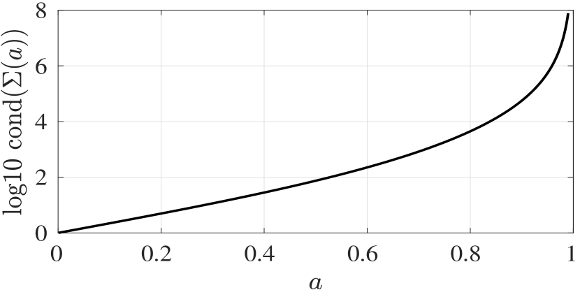
(a)

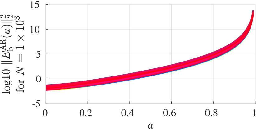
(b)

Figure 1: Profile of $\log_{10}[\operatorname*{cond}(\Sigma(a))]$ and $\log_{10}[\|E_{\operatorname*{b}}^{\operatorname*{AR}}(a)\|_{2}^{2}]$ for ridge regression with filtered white noise inputs. Panel (a): $\log_{10}[\operatorname*{cond}(\Sigma(a))]$ with $\mathcal{I}_{diff}(\operatorname*{cond}(\Sigma(a(i))))=0$ for $i=1,\cdots,990$. Panel (b): $\log_{10}[\|E_{\operatorname*{b}}^{\operatorname*{AR}}(a)\|_{2}^{2}]$ for $100$ test systems and $N=10^{3}$ with $\mathcal{I}_{diff}(\|E_{\operatorname*{b}}^{\operatorname*{AR}}(a(i))\|_{2}^{2})=0$ for $i=1,\cdots,990$. Note that the tendency of $\log_{10}[\|E_{\operatorname*{b}}^{\operatorname*{AR}}(a)\|_{2}^{2}]$ for $N=10^{5}$ is the same as that for $N=10^{3}$ and thus omitted.

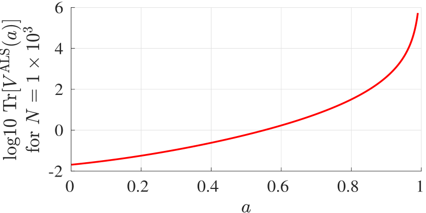
(a)

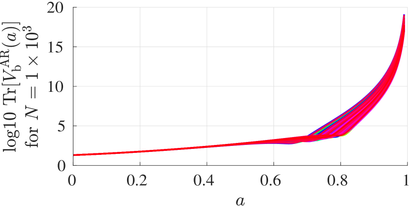
(b)

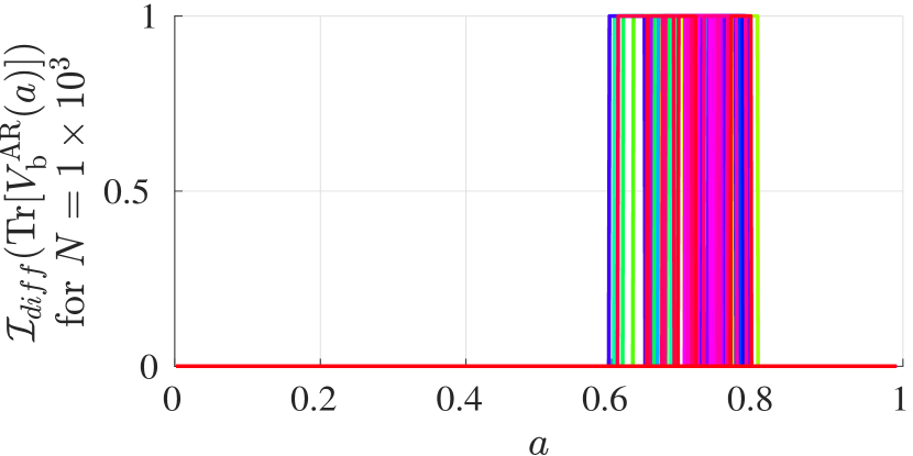
(c)

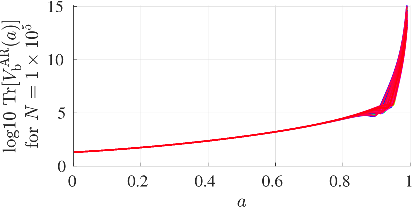
(d)

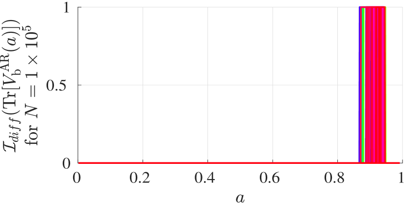
(e)

Figure 2: Profile of $\log_{10}\{\operatorname*{Tr}[V^{\operatorname*{ALS}}(a)]\}$ and $\log_{10}\{\operatorname*{Tr}[V_{\operatorname*{b}}^{\operatorname*{AR}}(a)]\}$ for ridge regression with filtered white noise inputs and $100$ test systems. Panel (a): $\log_{10}\{\operatorname*{Tr}[V^{\operatorname*{ALS}}(a)]\}$ for $N=10^{3}$ ($\mathcal{I}_{diff}(\operatorname*{Tr}[V^{\operatorname*{ALS}}(a(i))])=0$ for $i=1,\cdots,990$). Note that the tendency of $\log_{10}\{\operatorname*{Tr}[V^{\operatorname*{ALS}}(a)]\}$ for $N=10^{5}$ is similar to that for $N=10^{3}$ and is omitted. Panel (b): $\log_{10}\{\operatorname*{Tr}[V_{\operatorname*{b}}^{\operatorname*{AR}}(a)]\}$ for $N=10^{3}$. Panel (c): $\mathcal{I}_{diff}(\operatorname*{Tr}[V_{\operatorname*{b}}^{\operatorname*{AR}}(a)])$ for $N=10^{3}$. Panel (d): $\log_{10}\{\operatorname*{Tr}[V_{\operatorname*{b}}^{\operatorname*{AR}}(a)]\}$ for $N=10^{5}$. Panel (e): $\mathcal{I}_{diff}(\operatorname*{Tr}[V_{\operatorname*{b}}^{\operatorname*{AR}}(a)])$ for $N=10^{5}$.

6.2 Verification of Theorems 1-3 and Corollaries 2-3

6.2.1 Test Systems

We consider two types of test systems, where the first one is T1 as introduced in Section 6.1.1 and the second one is referred to as T2. For T2, we generate each test system as follows: first generate a $30$th order random system using the approach in [6] with its $5$ poles with largest modulus falling in $[0.94,0.96]$ and then truncate its impulse response to a finite one at the order $20$. For each type, we generate $100$ test systems, each of which has an FIR model with order $20$. The impulse response of each test system is then multiplied by a constant such that $\|\theta_{0}\|_{2}=10$ with $\theta_{0}$ defined in (8).

6.2.2 Test Data-bank

For each test system, we generate the test input signal $u(t)$ as a filtered white noise as described in Assumption 1, where $e(t)$ is chosen to be i.i.d. Gaussian distributed with mean zero and $\sigma_{e}^{2}=1$. Noting that the filter $H(q)$ in (99) depends on the choice of $a$ and $c_{u}$, we consider the following values of $a=0.05$, $0.7$ and $0.95$, and

• for T1, consider $c_{u}^{2}=0.02$, $0.1$ and $0.5$;

• for T2, consider $c_{u}^{2}=1$, $10$ and $100$.

For each value of $a$ and $c_{u}^{2}$, we then simulate each test system with the generated test input signal to get the noise-free output and then corrupt it with an additive measurement noise $v(t)$, which is Gaussian distributed with mean 0 and variance $\sigma^{2}=1$, leading to the measurement output, and as a result, we collect a data record with $10^{3}$ pairs of input and measurement output. For each value of $a$ and $c_{u}^{2}$ and for each test system, the above procedure is repeated for $6\times 10^{5}$ times, leading to $6\times 10^{5}$ data records. Therefore, for each test system, there are in total 9 data collections, each with $6\times 10^{5}$ data records.

6.2.3 Simulation Setup

For each test system of type T1 and its associated data collections, we consider the RLS estimator (12) with $P=\eta I_{n}$. For each test system of type T2 and its associated data collections, we consider the RLS estimator (12) with the TC kernel (14).

For both cases, the FIR model order $n$ is chosen to be $20$, i.e., $n=20$, the hyper-parameters are estimated using the $\operatorname*{EB}$ method (19a) and the noise variance $\sigma^{2}$ is estimated by (18), and moreover, we have the sample size $N=10^{3}$.

6.2.4 Simulation Results and Discussions

In Table 1, for $a\in{\mathbb{R}}$ and $b\in{\mathbb{Z}}$, we use $a\text{E}b$ to denote $a\times 10^{\operatorname*{b}}$ for convenience.

• Condition numbers of $\Phi^{T}\Phi$ and $\Sigma$

  Table 1: Condition number of $\Sigma$ and average condition numbers of $\Phi^{T}\Phi$ for different values of $a$ over the $6\times 10^{5}$ data records.

  $a$	$0.05$	$0.7$	$0.95$
  $\operatorname*{cond}(\Phi^{T}\Phi)$	2.00	9.10E2	5.98E5
  $\operatorname*{cond}(\Sigma)$	1.49	8.34E2	5.51E5

  As shown in Table 1, as $a$ increases, both $\operatorname*{cond}(\Phi^{T}\Phi)$ for fixed $N$ and $\operatorname*{cond}(\Sigma)$ increase, i.e. $\Phi^{T}\Phi$ and $\Sigma$ become more ill-conditioned.

• Verification of Theorem 1 and Corollary 2

  Fig. 3 shows that for both the ridge regression and the TC kernel,

  • for fixed $c_{u}^{2}$, the larger $a$, the larger the average squared norm of mean and the average variance of $\hat{\eta}_{\operatorname*{EB}}-\eta_{\operatorname*{b}}^{*}$;

  • for fixed $a$, the larger $c_{u}^{2}$, the smaller the average squared norm of mean and the average variance of $\hat{\eta}_{\operatorname*{EB}}-\eta_{\operatorname*{b}}^{*}$;

  • for fixed $a$ and $c_{u}^{2}$, the average variance of $\hat{\eta}_{\operatorname*{EB}}$ is quite close to $\operatorname*{Tr}[V_{\operatorname*{b}}^{\operatorname*{H}}(\eta_{\operatorname*{b}}^{*})]/N$.

  

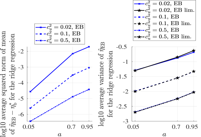
  (a)

  

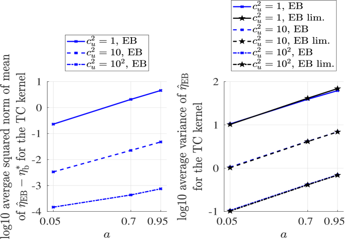
  (b)

  Figure 3: Profile of logarithm base $10$ average squared norm of mean of $\hat{\eta}_{\operatorname*{EB}}-\eta^{*}_{\operatorname*{b}}$ and variance of $\hat{\eta}_{\operatorname*{EB}}$ for the ridge regression and the TC kernel over $9$ data collections. Panel (a): Logarithm base $10$ of average squared norm of mean of $\hat{\eta}_{\operatorname*{EB}}-\eta^{*}_{\operatorname*{b}}$ and average variance of $\hat{\eta}_{\operatorname*{EB}}$ for the ridge regression (“ EB lim.” denotes $V_{\operatorname*{b}}^{\operatorname*{H}}(\eta_{\operatorname*{b}}^{*})/N$ and $V_{\operatorname*{b}}^{\operatorname*{H}}(\eta_{\operatorname*{b}}^{*})$ is defined as (109)). Panel (b): Logarithm base $10$ of average squared norm of mean of $\hat{\eta}_{\operatorname*{EB}}-\eta^{*}_{\operatorname*{b}}$ and average variance of $\hat{\eta}_{\operatorname*{EB}}$ for the TC kernel (“ EB lim.” denotes $\operatorname*{Tr}[V_{\operatorname*{b}}^{\operatorname*{H}}(\eta_{\operatorname*{b}}^{*})]/N$ and $V_{\operatorname*{b}}^{\operatorname*{H}}(\eta_{\operatorname*{b}}^{*})$ is defined as (40)).

• Verification of Theorems 2-3 and Corollary 3

  Since $\operatorname*{MSE}_{g}(\hat{\theta}^{\operatorname*{R}}(\hat{\eta}_{\operatorname*{EB}}))$ has no closed form expression, in order to assess the accuracy of the high order asymptotic distributions (46), (67) and (3), we calculate for each test system the sample average of ${\operatorname*{MSE}}_{g}(\hat{\theta}^{\operatorname*{R}}(\hat{\eta}_{\operatorname*{EB}}))$ over its associated $6\times 10^{5}$ Monte Carlo simulations and denote it by ${\operatorname*{SMSE}}_{g}(\hat{\theta}^{\operatorname*{R}}(\hat{\eta}_{\operatorname*{EB}}))$. Moreover, we let

  • ${\mathcal{S}_{1}}$ denote the number of systems satisfying

    $$\left|{\text{AMSE}_{g}^{\operatorname*{b},2}(\eta_{\operatorname*{b}}^{*})}-{\operatorname*{SMSE}}_{g}(\hat{\theta}^{\operatorname*{R}}(\hat{\eta}_{\operatorname*{EB}}))\right|$$

    $$< \left|{\text{AMSE}_{g}^{\operatorname*{b},1}(\eta_{\operatorname*{b}}^{*})}-{\operatorname*{SMSE}}_{g}(\hat{\theta}^{\operatorname*{R}}(\hat{\eta}_{\operatorname*{EB}}))\right|;$$ (118)

  • ${\mathcal{S}_{2}}$ denote the number of systems satisfying

    $$\left|{\text{AMSE}_{g}^{\operatorname*{b},3}(\eta_{\operatorname*{b}}^{*})}-{\operatorname*{SMSE}}_{g}(\hat{\theta}^{\operatorname*{R}}(\hat{\eta}_{\operatorname*{EB}}))\right|$$

    $$< \left|{\text{AMSE}_{g}^{\operatorname*{b},1}(\eta_{\operatorname*{b}}^{*})}-{\operatorname*{SMSE}}_{g}(\hat{\theta}^{\operatorname*{R}}(\hat{\eta}_{\operatorname*{EB}}))\right|;$$ (119)

  • ${\mathcal{S}_{3}}$ denote the number of systems satisfying

    $$\left|{\text{AMSE}_{g}^{\operatorname*{b},3}(\eta_{\operatorname*{b}}^{*})}-{\operatorname*{SMSE}}_{g}(\hat{\theta}^{\operatorname*{R}}(\hat{\eta}_{\operatorname*{EB}}))\right|$$

    $$< \left|{\text{AMSE}_{g}^{\operatorname*{b},2}(\eta_{\operatorname*{b}}^{*})}-{\operatorname*{SMSE}}_{g}(\hat{\theta}^{\operatorname*{R}}(\hat{\eta}_{\operatorname*{EB}}))\right|,$$ (120)

  among the 100 test systems, where ${\text{AMSE}_{g}^{\operatorname*{b},m}(\eta_{\operatorname*{b}}^{*})}$ with $m=1,2,3$ are defined in (97). Clearly,

  • the closer ${\mathcal{S}_{1}}$ or ${\mathcal{S}_{2}}$ to 100, the more accurate the high order asymptotic distributions (67) or (3) over the first order one (46);

  • the closer ${\mathcal{S}_{3}}$ to 100, the more accurate the third order asymptotic distributions (3) over the second order one (67).

  

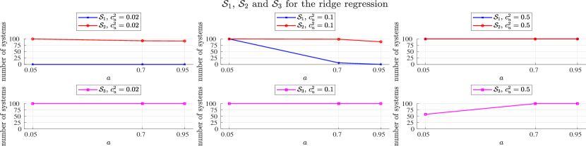
  (a)

  

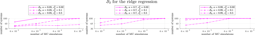
  (b)

  

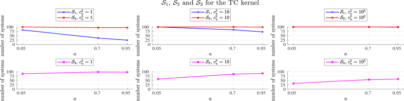
  (c)

  

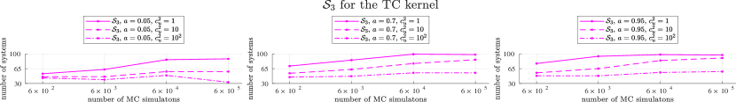
  (d)

  Figure 4: Profile of ${\mathcal{S}_{1}}$ (118), ${\mathcal{S}_{2}}$ (119) and ${\mathcal{S}_{3}}$ (120) for the ridge regression and the TC kernel. Panel (a): ${\mathcal{S}_{1}}$ and ${\mathcal{S}_{2}}$ (the first row), and ${\mathcal{S}_{3}}$ (the second row) for the ridge regression over $9$ data collections. Panel (b): ${\mathcal{S}_{3}}$ for the ridge regression over different numbers of data records. Panel (c): ${\mathcal{S}_{1}}$ and ${\mathcal{S}_{2}}$ (the first row), and ${\mathcal{S}_{3}}$ (the second row) for the TC kernel over $9$ data collections. Panel (d): ${\mathcal{S}_{3}}$ for TC kernel over different numbers of data records.

  Fig. 4 shows that for both the ridge regression and the TC kernel:

  • for fixed $c_{u}^{2}$, as $a$ increases, ${\mathcal{S}_{1}}$ and ${\mathcal{S}_{2}}$ tend to become smaller, and ${\mathcal{S}_{3}}$ tends to become larger (except when $a=0.95$ for the TC kernel);

  • for fixed $a$, as $c_{u}^{2}$ increases, ${\mathcal{S}_{1}}$ and ${\mathcal{S}_{2}}$ tend to become larger, and ${\mathcal{S}_{3}}$ tends to become smaller.

  For the ridge regression and TC kernel, the sums of ${\mathcal{S}_{2}}$ for all values of $a$ and $c_{u}^{2}$ are $873$ and $891$, respectively. It means that in contrast with the first order asymptotic distribution (46), there are $873$ cases for the ridge regression, and $891$ cases for the TC kernel, out of the total 900 cases ($9$ data collections) such that the third order one (3) is more accurate. Moreover, ${\mathcal{S}_{1}}$ is smaller or equal to ${\mathcal{S}_{2}}$ for both the ridge regression and the TC kernel. It indicates that the second order one (67) is less accurate, when $a$ is large or $c_{u}^{2}$ is small. This observation is reasonable, because it does not take into account the influence of the regularization, whose role is critical especially when the quality of the data is bad, i.e., when $a$ is large or $c_{u}^{2}$ is small.

  For the ridge regression and TC kernel, the sums of ${\mathcal{S}_{3}}$ for all values of $a$ and $c_{u}^{2}$ are $858$ and $663$, respectively. It means that in contrast with the second order asymptotic distribution (67), there are $858$ cases for the ridge regression, and $663$ cases for the TC kernel, out of the total 900 cases such that the third order one (3) is more accurate, especially when $a$ is large or $c_{u}^{2}$ is small. Moreover, the second order one (67) seems to become more accurate when the quality of the data is getting better, i.e., when $a$ becomes smaller or $c_{u}^{2}$ becomes larger. This observation is somewhat against our intuition that the third order one (3) should be better, and the reasons might be two-fold:

  • First, this may be due to the insufficient number of Monte Carlo simulations. Note that when $a$ becomes smaller or $c_{u}^{2}$ becomes larger, the quality of the data becomes better and thus not only $\operatorname*{MSE}_{g}(\hat{\theta}^{\operatorname*{R}}(\hat{\eta}_{\operatorname*{EB}}))$ but also its high order asymptotic approximations ${\text{AMSE}_{g}^{\operatorname*{b},m}(\eta_{\operatorname*{b}}^{*})}$, $m=1,2,3$ all become smaller, implying that the differences between them also become smaller. Therefore, we need more Monte Carlo simulations to obtain a more accurate approximation of $\operatorname*{MSE}_{g}(\hat{\theta}^{\operatorname*{R}}(\hat{\eta}_{\operatorname*{EB}}))$ to differentiate them. This tendency can be seen from most cases in the Panel (b) and Panel (d) in Fig. 4, where we display the performances as we increase the number of Monte Carlo simulations to $6\times 10^{5}$.

  • Second, this may also be due to that the sample size $N=10^{3}$ might not be large enough such that the approximation error of the terms involved might not be negligible when assessing the difference between ${\operatorname*{SMSE}}_{g}(\hat{\theta}^{\operatorname*{R}}(\hat{\eta}_{\operatorname*{EB}}))$ and ${\text{AMSE}_{g}^{\operatorname*{b},m}(\eta_{\operatorname*{b}}^{*})}$, $m=1,2,3$. In addition, it is also worth to note that the third order asymptotic distribution (3) has an extra term $\sqrt{N}(\widehat{\sigma^{2}}-\sigma^{2})$ in contrast with the second order one (67).

• For reference, we also assess the performance of the RLS estimator $\hat{\theta}^{\operatorname*{R}}(\hat{\eta}_{\operatorname*{EB}})$ from the perspective of $\operatorname*{MSE}_{g}$ with the “model fit” [15]:

  $$\text{Fit}_{g}=100\times\left(1-\frac{\|\hat{\theta}^{\operatorname*{R}}(\hat{\eta}_{\operatorname*{EB}})-\theta_{0}\|_{2}}{\|\theta_{0}-\overline{\theta_{0}}\|_{2}}\right),\overline{\theta_{0}}=\frac{1}{n}\sum_{i=1}^{n}g_{i}^{0}.$$

  In fact, the mean of $\text{Fit}_{g}$ can be seen as a normalized version of $\operatorname*{SMSE}_{g}(\hat{\theta}^{\operatorname*{R}}(\hat{\eta}_{\operatorname*{EB}}))$, which is equal to the sum of the squared norm of mean of $\hat{\theta}^{\operatorname*{R}}(\hat{\eta}_{\operatorname*{EB}})-\theta_{0}$, and the variance of $\hat{\theta}^{\operatorname*{R}}(\hat{\eta}_{\operatorname*{EB}})$. Fig. 5 shows that for both the ridge regression and the TC kernel,

  • for fixed $c_{u}^{2}$, the larger $a$, the smaller the average mean of $\text{Fit}_{g}$ of $\hat{\theta}^{\operatorname*{R}}(\hat{\eta}_{\operatorname*{EB}})$;

  • for fixed $a$, the larger $c_{u}^{2}$, the larger the average mean of $\text{Fit}_{g}$ of $\hat{\theta}^{\operatorname*{R}}(\hat{\eta}_{\operatorname*{EB}})$.

  

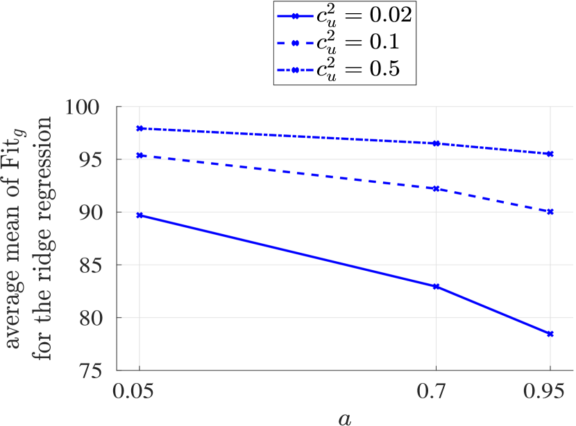
  (a)

  

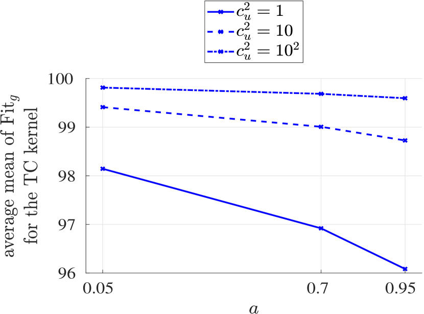
  (b)

  Figure 5: Profile of average mean of $\text{Fit}_{g}$ for the ridge regression and the TC kernel over $9$ data collections. Panel (a): Average mean of $\text{Fit}_{g}$ for the ridge regression. Panel (b): Average mean of $\text{Fit}_{g}$ for the TC kernel.

7 Conclusion

Asymptotic theory is a core component for the theory of system identification. In this paper, we studied the asymptotic theory for the regularized system identification, and in particular, the regularized finite impulse response (FIR) model estimation with the input signal chosen to be filtered white noise and the hyper-parameter estimator chosen to be the empirical Bayes (EB) method. Our obtained results on the convergence in distribution of the EB hyper-parameter estimator and on the high order asymptotic distributions of the corresponding kernel-based regularized least squares (RLS) estimator, expose the factors (e.g., the regression matrix and the kernel matrix) that affect the convergence properties of the EB hyper-parameter estimator and the corresponding RLS estimator. These results provide theoretical support to the widely observed numerical simulation results that the more ill-conditioned the regression matrix, the more slowly the EB hyper-parameter estimator and the corresponding RLS estimator converge to their limits, respectively. These results fill the gaps in the asymptotic theory for the regularized system identification, and have many potential applications, e.g., in finding the confidence intervals of the EB hyper-parameter estimator and the corresponding RLS model estimator.

Appendix A

Proofs of theorems, propositions and corollaries are included in Appendix A, among which proofs of Corollaries 1-3 are omitted because of the limitation of space.

A.1 Proof of Theorem 1

First, let

$$\overline{\mathscr{F}_{\operatorname*{EB}}}(\eta)= \widehat{\mathscr{F}_{\operatorname*{EB}}}(\eta)-(N-n)-(N-n)\log\widehat{\sigma^{2}}$$

$$-\log\det(\Phi^{T}\Phi)$$ (A.1)

$$= (\hat{\theta}^{\operatorname*{LS}})^{T}\hat{S}(\eta)^{-1}\hat{\theta}^{\operatorname*{LS}}+\log\det(\hat{S}(\eta)),$$ (A.2)

where $\hat{S}(\eta)$ is defined in (32). Since the difference between $\widehat{\mathscr{F}_{\operatorname*{EB}}}(\eta)$ in (A.1) and $\overline{\mathscr{F}_{\operatorname*{EB}}}(\eta)$ in (19b) is irrespective of $\eta$, we have $\hat{\eta}_{\operatorname*{EB}}=\operatorname*{arg\,min}_{\eta\in\Omega}\overline{\mathscr{F}_{\operatorname*{EB}}}(\eta)$. Using the analogous idea in the proof of [21, Theorem 1], we can apply (25)-(27), (38) and [21, Lemma B3] to derive (23).

Then we will derive the convergence in distribution of $\sqrt{N}(\hat{\eta}_{\operatorname*{EB}}-\eta_{\operatorname*{b}}^{*})$ based on the first-order Taylor expansion of ${\partial\overline{\mathscr{F}_{\operatorname*{EB}}}}/{\partial\eta}|_{\eta=\hat{\eta}_{\operatorname*{EB}}}$ around $\eta_{\operatorname*{b}}^{*}$ as follows,

$$0=\left.\frac{\partial\overline{\mathscr{F}_{\operatorname*{EB}}}}{\partial\eta}\right|_{\eta=\hat{\eta}_{\operatorname*{EB}}}=\left.\frac{\partial\overline{\mathscr{F}_{\operatorname*{EB}}}}{\partial\eta}\right|_{\eta=\eta_{\operatorname*{b}}^{*}}+\left.\frac{\partial^{2}\overline{\mathscr{F}_{\operatorname*{EB}}}}{\partial\eta\partial\eta^{T}}\right|_{\eta=\overline{\eta}_{N}}(\hat{\eta}_{\operatorname*{EB}}-\eta_{\operatorname*{b}}^{*}),$$

where the remainder term is represented in the Lagrange’s form and $\overline{\eta}_{N}$ belongs to a neighborhood of $\eta_{\operatorname*{b}}^{*}$ with radius $\|\hat{\eta}_{\operatorname*{EB}}-\eta_{\operatorname*{b}}^{*}\|_{2}$. It follows that

$$\sqrt{N}(\hat{\eta}_{\operatorname*{EB}}-\eta_{\operatorname*{b}}^{*})=-\left(\left.\frac{\partial^{2}\overline{\mathscr{F}_{\operatorname*{EB}}}}{\partial\eta\partial\eta^{T}}\right|_{\eta=\overline{\eta}_{N}}\right)^{-1}\left(\sqrt{N}\left.\frac{\partial\overline{\mathscr{F}_{\operatorname*{EB}}}}{\partial\eta}\right|_{\eta=\eta_{\operatorname*{b}}^{*}}\right),$$ (A.3)

where if $\left.{\partial^{2}\overline{\mathscr{F}_{\operatorname*{EB}}}}/{\partial\eta\partial\eta^{T}}\right|_{\eta=\overline{\eta}_{N}}$ is not positive definite for small $N$, the pseudo inverse could be used instead.

Now, in what follows, we consider the almost sure convergence of $\left.{\partial^{2}\overline{\mathscr{F}_{\operatorname*{EB}}}}/{\partial\eta\partial\eta^{T}}\right|_{\eta=\overline{\eta}_{N}}$ and the convergence in distribution of $\sqrt{N}\left.{\partial\overline{\mathscr{F}_{\operatorname*{EB}}}}/{\partial\eta}\right|_{\eta=\eta_{\operatorname*{b}}^{*}}$.

1. Firstly, we show in two steps that

   $$\left.\frac{\partial^{2}\overline{\mathscr{F}_{\operatorname*{EB}}}}{\partial\eta\partial\eta^{T}}\right|_{\eta=\overline{\eta}_{N}}\overset{a.s.}{\to}\left.\frac{\partial^{2}W_{\operatorname*{b}}}{\partial\eta\partial\eta^{T}}\right|_{\eta=\eta^{*}_{\operatorname*{b}}}=A_{\operatorname*{b}}(\eta_{\operatorname*{b}}^{*})\succ 0,$$ (A.4)

   where $A_{\operatorname*{b}}(\eta_{\operatorname*{b}}^{*})$ is defined in (1). The first step is to prove

   $$\overline{\eta}_{N}\overset{a.s.}{\to}\eta_{\operatorname*{b}}^{*},$$ (A.5)

   which is true because $\|\overline{\eta}_{N}-\eta_{\operatorname*{b}}^{*}\|_{2}\leq\|\hat{\eta}_{\operatorname*{EB}}-\eta_{\operatorname*{b}}^{*}\|_{2}\overset{a.s.}{\to}0$. The second step is to prove that ${\partial^{2}\overline{\mathscr{F}_{\operatorname*{EB}}}}/{\partial\eta\partial\eta^{T}}$ converges to ${\partial^{2}W_{\operatorname*{b}}}/{\partial\eta\partial\eta^{T}}$ almost surely and uniformly. Their $(k,l)$th elements are

   $$\frac{\partial^{2}\overline{\mathscr{F}_{\operatorname*{EB}}}}{\partial\eta_{k}\partial\eta_{l}}= (\hat{\theta}^{\operatorname*{LS}})^{T}\frac{\partial^{2}\hat{S}^{-1}}{\partial\eta_{k}\partial\eta_{l}}\hat{\theta}^{\operatorname*{LS}}+\operatorname*{Tr}\left(\frac{\partial\hat{S}^{-1}}{\partial\eta_{l}}\frac{\partial P}{\partial\eta_{k}}\right)$$

   $$+\operatorname*{Tr}\left(\hat{S}^{-1}\frac{\partial^{2}P}{\partial\eta_{k}\partial\eta_{l}}\right),$$ (A.6)

   $$\frac{\partial^{2}W_{\operatorname*{b}}}{\partial\eta_{k}\partial\eta_{l}}= \theta_{0}^{T}\frac{\partial^{2}P^{-1}}{\partial\eta_{k}\partial\eta_{l}}\theta_{0}+\operatorname*{Tr}\left(\frac{\partial P^{-1}}{\partial\eta_{l}}\frac{\partial P}{\partial\eta_{k}}\right)$$

   $$+\operatorname*{Tr}\left(P^{-1}\frac{\partial^{2}P}{\partial\eta_{k}\partial\eta_{l}}\right).$$ (A.7)

   Then their difference can be represented as

   $${\partial^{2}\overline{\mathscr{F}_{\operatorname*{EB}}}}/{\partial\eta_{k}\partial\eta_{l}}-{\partial^{2}W_{\operatorname*{b}}}/{\partial\eta_{k}\partial\eta_{l}}= \Psi_{1,\operatorname*{b}}+\operatorname*{Tr}(\Psi_{2,\operatorname*{b}}),$$

   where

   $$\Psi_{1,\operatorname*{b}}= (\hat{\theta}^{\operatorname*{LS}}-\theta_{0})^{T}\frac{\partial^{2}\hat{S}^{-1}}{\partial\eta_{k}\partial\eta_{l}}\hat{\theta}^{\operatorname*{LS}}+\theta_{0}^{T}\frac{\partial^{2}P^{-1}}{\partial\eta_{k}\partial\eta_{l}}(\hat{\theta}^{\operatorname*{LS}}-\theta_{0})$$

   $$+\theta_{0}^{T}\left(\frac{\partial^{2}\hat{S}^{-1}}{\partial\eta_{k}\partial\eta_{l}}-\frac{\partial^{2}P^{-1}}{\partial\eta_{k}\partial\eta_{l}}\right)\hat{\theta}^{\operatorname*{LS}},$$

   $$\Psi_{2,\operatorname*{b}}= \left(\frac{\partial\hat{S}^{-1}}{\partial\eta_{l}}-\frac{\partial P^{-1}}{\partial\eta_{l}}\right)\frac{\partial P}{\partial\eta_{k}}+(\hat{S}^{-1}-P^{-1})\frac{\partial^{2}P}{\partial\eta_{k}\partial\eta_{l}}.$$

   Under Assumption 5, there exists a compact subset $\widetilde{\Omega}_{1}$ of $\Omega$ such that $\eta_{\operatorname*{b}}^{*}\in\widetilde{\Omega}_{1}\subset\Omega$ and moreover, for any $k,l=1,\cdots,p$,

   $$\|P\|_{F},\ \|\hat{S}^{-1}\|_{F}<\|P^{-1}\|_{F}\ \text{are}\ \text{bounded},$$ (A.8a)

   $$\left\|{\partial P}/{\partial\eta_{l}}\right\|_{F},\ \left\|{\partial^{2}P}/{\partial\eta_{k}\partial\eta_{l}}\right\|_{F}\ \text{are}\ \text{bounded}.$$ (A.8b)

   According to [22, (59) p. 9], we can see that both ${\partial^{2}P^{-1}}/{\partial\eta_{k}\partial\eta_{l}}$ and ${\partial^{2}\hat{S}^{-1}}/{\partial\eta_{k}\partial\eta_{l}}$ are made of $P^{-1}$, $\hat{S}^{-1}$, ${\partial P}/{\partial\eta_{k}}$, ${\partial P}/{\partial\eta_{l}}$ and ${\partial^{2}P}/{\partial\eta_{k}\partial\eta_{l}}$. Hence, using (A.8), (38), [22, (59) p. 9] and matrix norm inequalities in [22, p. 61-62], there exists a constant $M_{1}>0$, irrespective of $N$, such that,

   $$\sup_{\eta\in\widetilde{\Omega}_{1}}|\Psi_{1,\operatorname*{b}}|\leq \|\hat{\theta}^{\operatorname*{LS}}-\theta_{0}\|_{2}\sup_{\eta\in\widetilde{\Omega}_{1}}\left\|\frac{\partial^{2}\hat{S}^{-1}}{\partial\eta_{k}\partial\eta_{l}}\right\|_{F}\|\hat{\theta}^{\operatorname*{LS}}\|_{2}$$

   $$+\|\theta_{0}\|_{2}\sup_{\eta\in\widetilde{\Omega}_{1}}\left\|\frac{\partial^{2}\hat{S}^{-1}}{\partial\eta_{k}\partial\eta_{l}}-\frac{\partial^{2}P^{-1}}{\partial\eta_{k}\partial\eta_{l}}\right\|_{F}\|\hat{\theta}^{\operatorname*{LS}}\|_{2}$$

   $$+\|\theta_{0}\|_{2}\sup_{\eta\in\widetilde{\Omega}_{1}}\left\|\frac{\partial^{2}P^{-1}}{\partial\eta_{k}\partial\eta_{l}}\right\|_{F}\|\hat{\theta}^{\operatorname*{LS}}-\theta_{0}\|_{2}$$

   $$\leq M_{1}\|\hat{\theta}^{\operatorname*{LS}}-\theta_{0}\|_{2}\|\hat{\theta}^{\operatorname*{LS}}\|_{2}$$

   $$+M_{1}\frac{1}{N}\|\theta_{0}\|_{2}\widehat{\sigma^{2}}\|N(\Phi^{T}\Phi)^{-1}\|_{F}\|\hat{\theta}^{\operatorname*{LS}}\|_{2}$$

   $$+M_{1}\|\theta_{0}\|_{2}\|\hat{\theta}^{\operatorname*{LS}}-\theta_{0}\|_{2}\overset{a.s.}{\to}0,$$ (A.9)

   where the almost sure convergence can be proved using (25)-(27), the continuous mapping theorem [28, Theorem 2.3] and Slutsky’s theorem [28, Theorem 2.8]. Similarly, it can be shown that there exists a constant $M_{2}>0$, irrespective of $N$, such that

   $$\sup_{\eta\in\widetilde{\Omega}_{1}}|\operatorname*{Tr}(\Psi_{2,\operatorname*{b}})|\leq M_{2}\widehat{\sigma^{2}}\|N(\Phi^{T}\Phi)^{-1}\|_{F}/N\overset{a.s.}{\to}0.$$

   Since both $\Psi_{1,\operatorname*{b}}$ and $\operatorname*{Tr}(\Psi_{2,\operatorname*{b}})$ converge to zero almost surely and uniformly in $\widetilde{\Omega}_{1}$, we have

   $$\sup_{\eta\in\widetilde{\Omega}_{1}}\left|{\partial^{2}\overline{\mathscr{F}_{\operatorname*{EB}}}}/{\partial\eta_{k}\partial\eta_{l}}-{\partial^{2}W_{\operatorname*{b}}}/{\partial\eta_{k}\partial\eta_{l}}\right|\overset{a.s.}{\to}0$$

   by the continuous mapping theorem [28, Theorem 2.3]. Finally, note that $\overline{\eta}_{N}\overset{a.s.}{\to}\eta_{\operatorname*{b}}^{*}$ and then by [14, Lemma B.17], we have (A.4), where the positive definiteness of $A_{\operatorname*{b}}(\eta_{\operatorname*{b}}^{*})$ is due to Assumption 7.

2. Secondly, we show that

   $$\sqrt{N}\left.{\partial\overline{\mathscr{F}_{\operatorname*{EB}}}}/{\partial\eta}\right|_{\eta=\eta_{\operatorname*{b}}^{*}}\overset{d.}{\to}\mathcal{N}(0,\sigma^{2}B_{\operatorname*{b}}(\eta_{\operatorname*{b}}^{*})\Sigma^{-1}B_{\operatorname*{b}}(\eta_{\operatorname*{b}}^{*})^{T}),$$ (A.10)

   where $B_{\operatorname*{b}}(\eta_{\operatorname*{b}}^{*})$ is defined in (42).

   The $k$th elements of ${\partial\overline{\mathscr{F}_{\operatorname*{EB}}}}/{\partial\eta}$ and ${\partial W_{\operatorname*{b}}}/{\partial\eta}$ are

   $$\frac{\partial\overline{\mathscr{F}_{\operatorname*{EB}}}}{\partial\eta_{k}}= (\hat{\theta}^{\operatorname*{LS}})^{T}\frac{\partial\hat{S}^{-1}}{\partial\eta_{k}}\hat{\theta}^{\operatorname*{LS}}+\operatorname*{Tr}\left(\hat{S}^{-1}\frac{\partial P}{\partial\eta_{k}}\right),$$ (A.11)

   $$\frac{\partial W_{\operatorname*{b}}}{\partial\eta_{k}}= \theta_{0}^{T}\frac{\partial P^{-1}}{\partial\eta_{k}}\theta_{0}+\operatorname*{Tr}\left(P^{-1}\frac{\partial P}{\partial\eta_{k}}\right).$$ (A.12)

   From Assumption 7 and (22a), we can see that $\eta_{\operatorname*{b}}^{*}$ should satisfy the first-order optimality condition, i.e. for $k=1,\cdots,p$, $\left.{\partial W_{\operatorname*{b}}}/{\partial\eta_{k}}\right|_{\eta=\eta_{\operatorname*{b}}^{*}}=0$. It leads to

   $$\sqrt{N}\left.\frac{\partial\overline{\mathscr{F}_{\operatorname*{EB}}}}{\partial\eta_{k}}\right|_{\eta=\eta_{\operatorname*{b}}^{*}}= \sqrt{N}\left.\left(\frac{\partial\overline{\mathscr{F}_{\operatorname*{EB}}}}{\partial\eta_{k}}-\frac{\partial W_{\operatorname*{b}}}{\partial\eta_{k}}\right)\right|_{\eta=\eta_{\operatorname*{b}}^{*}}$$

   $$= [\Upsilon_{\operatorname*{b},1}]_{k}+[\Upsilon_{\operatorname*{b},2}]_{k},$$ (A.13)

   where for $k=1,\cdots,p$, the $k$th elements of $\Upsilon_{\operatorname*{b},1}\in{\mathbb{R}}^{p}$ and $\Upsilon_{\operatorname*{b},2}\in{\mathbb{R}}^{p}$ are

   $${\left[\Upsilon_{\operatorname*{b},1}\right]_{k}=}$$ (A.14)

   $${\left.\left[(\hat{\theta}^{\operatorname*{LS}})^{T}\frac{\partial\hat{S}^{-1}}{\partial\eta_{k}}+\theta_{0}^{T}\frac{\partial P^{-1}}{\partial\eta_{k}}\right]\right|_{\eta=\eta_{\operatorname*{b}}^{*}}N(\Phi^{T}\Phi)^{-1}\sqrt{N}\frac{\Phi^{T}V}{N},}$$

   $$\left[\Upsilon_{\operatorname*{b},2}\right]_{k}=\left.\theta_{0}^{T}\sqrt{N}\left(\frac{\partial\hat{S}^{-1}}{\partial\eta_{k}}-\frac{\partial P^{-1}}{\partial\eta_{k}}\right)\right|_{\eta=\eta_{\operatorname*{b}}^{*}}\hat{\theta}^{\operatorname*{LS}}$$

   $$\qquad\qquad+\left.\operatorname*{Tr}\left[\sqrt{N}(\hat{S}^{-1}-P^{-1})\frac{\partial P}{\partial\eta_{k}}\right]\right|_{\eta=\eta_{\operatorname*{b}}^{*}}.$$ (A.15)

   1. For $[\Upsilon_{\operatorname*{b},1}]_{k}$, using (26), (28), (35), the continuous mapping theorem [28, Theorem 2.3], Slutsky’s theorem [28, Theorem 2.8] and [28, Theorem 2.7], we have

      $$[\Upsilon_{\operatorname*{b},1}]_{k}\overset{d.}{\to}2\left[B_{\operatorname*{b}}(\eta^{*}_{\operatorname*{b}})\right]_{k,:}\Sigma^{-1}\upsilon,$$ (A.16)

      where $\left[B_{\operatorname*{b}}(\eta^{*}_{\operatorname*{b}})\right]_{k,:}$ denotes the $k$th row of $B_{\operatorname*{b}}(\eta^{*}_{\operatorname*{b}})$.

   2. For $[\Upsilon_{\operatorname*{b},2}]_{k}$, using (26), (34), (36), the continuous mapping theorem [28, Theorem 2.3], Slutsky’s theorem [28, Theorem 2.8] and [28, Theorem 2.7], it can be seen that

      $$[\Upsilon_{\operatorname*{b},2}]_{k}\overset{d.}{\to}0.$$ (A.17)

   It follows $\sqrt{N}\left.{\partial\overline{\mathscr{F}_{\operatorname*{EB}}}}/{\partial\eta_{k}}\right|_{\eta=\eta_{\operatorname*{b}}^{*}}\overset{d.}{\to}2\left[B_{\operatorname*{b}}(\eta^{*}_{\operatorname*{b}})\right]_{k,:}\Sigma^{-1}\upsilon$. Therefore,

   $$\sqrt{N}\left.{\partial\overline{\mathscr{F}_{\operatorname*{EB}}}}/{\partial\eta}\right|_{\eta=\eta_{\operatorname*{b}}^{*}}\overset{d.}{\to}2B_{\operatorname*{b}}(\eta_{\operatorname*{b}}^{*})\Sigma^{-1}\upsilon.$$ (A.18)

   Then noting ${\mathbb{E}}(\upsilon\upsilon^{T})=\sigma^{2}\Sigma^{-1}$ in (29c), the covariance matrix of its limiting distribution is nothing but $4\sigma^{2}B_{\operatorname*{b}}(\eta_{\operatorname*{b}}^{*})\Sigma^{-1}B_{\operatorname*{b}}(\eta_{\operatorname*{b}}^{*})^{T}$.

3. Lastly, we insert (A.4) and (A.10) into (A.3). Using Slutsky’s theorem, we complete the proof of (39).

A.2 Proof of Proposition 1

We apply (43) to $V_{\operatorname*{b}}^{\operatorname*{H}}(\eta_{\operatorname*{b}}^{*})$ in (40) to obtain

$$\operatorname*{Tr}[V_{\operatorname*{b}}^{\operatorname*{H}}(\eta_{\operatorname*{b}}^{*})]=\sum_{i=1}^{n}\frac{4\sigma^{2}}{\lambda_{i}(\Sigma)}e_{\Sigma,i}^{T}B_{\operatorname*{b}}(\eta_{\operatorname*{b}}^{*})^{T}A_{\operatorname*{b}}(\eta_{\operatorname*{b}}^{*})^{-2}B_{\operatorname*{b}}(\eta_{\operatorname*{b}}^{*})e_{\Sigma,i}.$$

Since $\eta_{\operatorname*{b}}^{*}$, as defined in (22), is irrespective of $\Sigma$ and only depends on $\theta_{0}$ and $P$, we can obtain that $\operatorname*{Tr}[V_{\operatorname*{b}}^{\operatorname*{H}}(\eta_{\operatorname*{b}}^{*})]$ increases if we fix $\lambda_{i}(\Sigma)$ for all $i=1,\cdots,n-1$ and decrease $\lambda_{n}(\Sigma)$, i.e., if we increase $\operatorname*{cond}(\Sigma)$. For bounds of $\operatorname*{Tr}[V_{\operatorname*{b}}^{\operatorname*{H}}(\eta_{\operatorname*{b}}^{*})]$, we use [14, (B.66) in Lemma B.23].

A.3 Proof of Proposition 2

We rewrite (12b) as

$$\hat{\theta}^{\operatorname*{R}}(\hat{\eta}_{\operatorname*{EB}})= \left[\Phi^{T}\Phi+\widehat{\sigma^{2}}P(\hat{\eta}_{\operatorname*{EB}})^{-1}\right]^{-1}\Phi^{T}Y$$

$$= P(\hat{\eta}_{\operatorname*{EB}})\hat{S}(\hat{\eta}_{\operatorname*{EB}})^{-1}(\Phi^{T}\Phi)^{-1}\Phi^{T}Y$$

$$= \left[\hat{S}(\hat{\eta}_{\operatorname*{EB}})-\widehat{\sigma^{2}}(\Phi^{T}\Phi)^{-1}\right]\hat{S}(\hat{\eta}_{\operatorname*{EB}})^{-1}(\Phi^{T}\Phi)^{-1}\Phi^{T}Y$$

$$= \theta_{0}+(\Phi^{T}\Phi)^{-1}\Phi^{T}V-\frac{1}{N}\widehat{\sigma^{2}}N(\Phi^{T}\Phi)^{-1}\hat{S}(\hat{\eta}_{\operatorname*{EB}})^{-1}\hat{\theta}^{\operatorname*{LS}}.$$ (A.19)

Moreover, under Assumption 6, using (A.8a), (23), (33) and [14, Lemma B.17], we have

$$\hat{S}(\hat{\eta}_{\operatorname*{EB}})^{-1}\overset{a.s.}{\to}P(\eta^{*}_{\operatorname*{b}})^{-1}.$$ (A.20)

Then applying (25), (26), (27), (28), (23), (A.19), (A.20), the continuous mapping theorem [28, Theorem 2.3], Slutsky’s theorem [28, Theorem 2.8] and [28, Theorem 2.7], we can conclude that $\sqrt{N}(\hat{\theta}^{\operatorname*{R}}(\hat{\eta}_{\operatorname*{EB}})-\theta_{0})\overset{d.}{\to}\mathcal{N}(0,V^{\operatorname*{ALS}}_{1})$.

A.4 Proof of Theorem 2

For $\sqrt{N}(\hat{\theta}^{\operatorname*{LS}}-\theta_{0})$, we can rewrite it as

$$\sqrt{N}(\hat{\theta}^{\operatorname*{LS}}-\theta_{0})=\sqrt{N}(\Phi^{T}\Phi)^{-1}\Phi^{T}V$$

$$= \Sigma^{-1}\sqrt{N}\frac{\Phi^{T}V}{N}+\left[N(\Phi^{T}\Phi)^{-1}-\Sigma^{-1}\right]\sqrt{N}\frac{\Phi^{T}V}{N},$$ (A.21)

which is nothing but (48)-(50). Since (48) contains two building blocks: $\sqrt{N}[N(\Phi^{T}\Phi)^{-1}-\Sigma^{-1}]$ and $\sqrt{N}\Phi^{T}V/N$, we can apply (28) together with (25), (26) and the continuous mapping theorem [28, Theorem 2.3] to derive (51)-(53). Moreover, according to (29) and [22, (511), (520) p. 60], we can obtain (58)-(64).

A.5 Proof of Theorem 3

For $\sqrt{N}(\hat{\theta}^{\operatorname*{R}}(\hat{\eta}_{\operatorname*{EB}})$ $-\theta_{0})$, we first decompose it using (A.19),

$$\sqrt{N}\left(\hat{\theta}^{\operatorname*{R}}(\hat{\eta}_{\operatorname*{EB}})-\theta_{0}\right)$$

$$= \hat{\theta}^{\operatorname*{ALS}}_{1}+\frac{1}{\sqrt{N}}\left(\hat{\theta}^{\operatorname*{ALS}}_{2}-\frac{1}{\sqrt{N}}\widehat{\sigma^{2}}N(\Phi^{T}\Phi)^{-1}\hat{S}(\hat{\eta}_{\operatorname*{EB}})^{-1}\hat{\theta}^{\operatorname*{LS}}\right),$$

where $\hat{\theta}^{\operatorname*{ALS}}_{1}$ and $\hat{\theta}^{\operatorname*{ALS}}_{2}$ have no more than first order expansions, and

$$-\frac{1}{\sqrt{N}}\widehat{\sigma^{2}}N(\Phi^{T}\Phi)^{-1}\hat{S}(\hat{\eta}_{\operatorname*{EB}})^{-1}\hat{\theta}^{\operatorname*{LS}}$$

$$= -\frac{1}{\sqrt{N}}\sigma^{2}\Sigma^{-1}P(\eta_{\operatorname*{b}}^{*})^{-1}\theta_{0}$$ (A.22)

$$-\frac{1}{N}\sqrt{N}\Big{[}\widehat{\sigma^{2}}N(\Phi^{T}\Phi)^{-1}\hat{S}(\hat{\eta}_{\operatorname*{EB}})^{-1}\hat{\theta}^{\operatorname*{LS}}-\sigma^{2}\Sigma^{-1}P(\eta_{\operatorname*{b}}^{*})^{-1}\theta_{0}\Big{]}.$$

It leads to the third order expansion of $\sqrt{N}(\hat{\theta}^{\operatorname*{R}}(\hat{\eta}_{\operatorname*{EB}})$ $-\theta_{0})$ as shown in (71).

To derive the third order asymptotic distribution of $\sqrt{N}(\hat{\theta}^{\operatorname*{R}}(\hat{\eta}_{\operatorname*{EB}})-\theta_{0})$, we decompose $\hat{\theta}^{\operatorname*{AR}}_{\text{b3}}$ in (3) as follows:

$$-\sqrt{N}\Big{[}\widehat{\sigma^{2}}N(\Phi^{T}\Phi)^{-1}\hat{S}(\hat{\eta}_{\operatorname*{EB}})^{-1}\hat{\theta}^{\operatorname*{LS}}-\sigma^{2}\Sigma^{-1}P(\eta_{\operatorname*{b}}^{*})^{-1}\theta_{0}\Big{]}$$

$$= -\left(\Xi_{\operatorname*{b},1}^{\operatorname*{AR}}+\Xi_{\operatorname*{b},2}^{\operatorname*{AR}}+\Xi_{\operatorname*{b},3}^{\operatorname*{AR}}+\Xi_{\operatorname*{b},4}^{\operatorname*{AR}}\right),$$ (A.23)

where

$$\Xi_{\operatorname*{b},1}^{\operatorname*{AR}}= \sqrt{N}(\widehat{\sigma^{2}}-\sigma^{2})N(\Phi^{T}\Phi)^{-1}\hat{S}(\hat{\eta}_{\operatorname*{EB}})^{-1}\hat{\theta}^{\operatorname*{LS}},$$

$$\Xi_{\operatorname*{b},2}^{\operatorname*{AR}}= \sigma^{2}{\sqrt{N}\left[N(\Phi^{T}\Phi)^{-1}-\Sigma^{-1}\right]}\hat{S}(\hat{\eta}_{\operatorname*{EB}})^{-1}\hat{\theta}^{\operatorname*{LS}},$$

$$\Xi_{\operatorname*{b},3}^{\operatorname*{AR}}= -\sigma^{2}\Sigma^{-1}\hat{S}(\hat{\eta}_{\operatorname*{EB}})^{-1}$$

$$\left[\sum_{k=1}^{p}\left.\frac{\partial P(\eta)}{\partial\eta_{k}}\right|_{\eta=\tilde{\eta}_{N}}e_{k}^{T}\sqrt{N}(\hat{\eta}_{\operatorname*{EB}}-\eta_{\operatorname*{b}}^{*})\right]P(\eta_{\operatorname*{b}}^{*})^{-1}\hat{\theta}^{\operatorname*{LS}}$$

$$+\sigma^{2}\Sigma^{-1}P(\eta_{\operatorname*{b}}^{*})^{-1}N(\Phi^{T}\Phi)^{-1}\sqrt{N}\Phi^{T}V/N,$$

$$\Xi_{\operatorname*{b},4}^{\operatorname*{AR}}= -\frac{1}{\sqrt{N}}\widehat{\sigma^{2}}\sigma^{2}\Sigma^{-1}\hat{S}(\hat{\eta}_{\operatorname*{EB}})^{-1}{N}(\Phi^{T}\Phi)^{-1}P(\eta_{\operatorname*{b}}^{*})^{-1}\hat{\theta}^{\operatorname*{LS}},$$

and for the derivation we use (3) and $\tilde{\eta}_{N}$ belongs to a neighborhood of $\eta^{*}_{\operatorname*{b}}$ with radius $\|\hat{\eta}_{\operatorname*{EB}}-\eta^{*}_{\operatorname*{b}}\|_{2}$.

• For $\Xi_{\operatorname*{b},1}^{\operatorname*{R}}$ and $\Xi_{\operatorname*{b},2}^{\operatorname*{AR}}$, it is clear that they contain building blocks $\sqrt{N}(\widehat{\sigma^{2}}-\sigma^{2})$ and $\sqrt{N}[N(\Phi^{T}\Phi)^{-1}-\Sigma^{-1}]$, respectively.

• For $\Xi_{\operatorname*{b},3}^{\operatorname*{AR}}$, inserting (A.3), (A.4) and (A.18) into $\sqrt{N}(\hat{\eta}_{\operatorname*{EB}}-\eta_{\operatorname*{b}}^{*})$, we can see that $\Xi_{\operatorname*{b},3}^{\operatorname*{AR}}$ contains the building block $\sqrt{N}\Phi^{T}V/N$.

• For $\Xi_{\operatorname*{b},4}^{\operatorname*{AR}}$, using (25), (26), (27), (A.20) and Slutsky’s theorem [28, Theorem 2.8], we have $\Xi_{\operatorname*{b},4}^{\operatorname*{AR}}\overset{a.s.}{\to}0$.

Hence, we can apply (28) together with (25), (26), (27), (A.20), [14, Lemma B.17], the continuous mapping theorem [28, Theorem 2.3], Slutsky’s theorem [28, Theorem 2.8] and [28, Theorem 2.7] to obtain (3)-(3), and

$$C_{\operatorname*{b}}(\eta_{\operatorname*{b}}^{*})= 2\left[\sum_{k=1}^{p}P(\eta_{\operatorname*{b}}^{*})^{-1}\left.\frac{\partial P(\eta)}{\partial\eta_{k}}\right|_{\eta=\eta_{\operatorname*{b}}^{*}}P(\eta_{\operatorname*{b}}^{*})^{-1}\theta_{0}e_{k}^{T}\right]$$

$$A_{\operatorname*{b}}(\eta_{\operatorname*{b}}^{*})^{-1}B_{\operatorname*{b}}(\eta_{\operatorname*{b}}^{*})+P(\eta_{\operatorname*{b}}^{*})^{-1}$$ (A.24)

can be rewritten as (75) using (42), [22, (59) p. 9], and the fact that for $e_{k}\in{\mathbb{R}}^{p}$, its $k$th element is one and others zero.

Moreover, according to (29) and [22, (511), (520) p. 60], we can obtain (82)-(94).

A.6 Proof of Proposition 3

It can be derived by using the EVD of $\Sigma$ in (43) and [14, Lemma B.23].

A.7 Proof of Lemma 2

To derive Lemma 2, we use Newton’s generalized binomial formula and formulas of mathematical series.

First, if we consider $H(q)$ in the form of (99), we have

$$H(q)=c_{u}\frac{1}{(1-aq^{-1})^{2}}=c_{u}\sum_{k=0}^{\infty}(k+1)a^{k}q^{-k},$$

which implies that the impulse response of $H(q)$ is $h(k)=c_{u}(k+1)a^{k}$ for $k\geq 0$ and $h(k)=0$ for $k<0$. Recall Newton’s generalized binomial formula, for any $|x|<1$, the following equality holds,

$$\frac{1}{(1-x)^{\alpha}}=\sum_{k=0}^{\infty}\left(\begin{array}[]{c}\alpha+k-1\\ k\end{array}\right)x^{k}.$$ (A.27)

Then it follows that for $\tau\in{\mathbb{Z}}$, we insert (7b) to obtain

$$R_{u}(\tau)= 2\sigma^{2}_{e}c_{u}^{2}a^{|\tau|}\sum_{k=0}^{\infty}\left[\frac{(k+1)(k+2)}{2}(a^{2})^{k}\right]$$

$$+(|\tau|-1)\sigma^{2}_{e}c_{u}^{2}a^{|\tau|}\sum_{k=0}^{\infty}\left[(k+1)(a^{2})^{k}\right]$$

$$= c_{u}^{2}\sigma_{e}^{2}a^{|\tau|}\left[\frac{2}{(1-a^{2})^{3}}+\frac{|\tau|-1}{(1-a^{2})^{2}}\right],$$ (A.28)

which is derived from (A.27) and $|a|<1$.

Then, by using formulas of mathematical series, we can insert (A.7) into each element of $\Sigma$ and (30) to obtain (106) and (• ‣ 2), respectively. Moreover, when $a=0$, we can obtain (101) and (105).

[]Yue Ju received her Bachelor degree from Nanjing University of Science $\&$ Technology in 2017 and her Ph.D. from the Chinese University of Hong Kong, Shenzhen, in 2022. She is now a postdoc at the Chinese University of Hong Kong, Shenzhen and Shenzhen Research Institute of Big Data. She has been mainly working in the area of system identification. []Biqiang Mu received the Bachelor of Engineering degree from Sichuan University and the Ph.D. degree in Operations Research and Cybernetics from the Academy of Mathematics and Systems Science, Chinese Academy of Sciences. He was a postdoc at the Wayne State University, the Western Sydney University, and the Linköping University, respectively. He is currently an associate professor at the Academy of Mathematics and Systems Science, Chinese Academy of Sciences. His research interests include system identification, machine learning, and their applications. [] Lennart Ljung received his PhD in Automatic Control from Lund Institute of Technology in 1974. Since 1976 he is Professor of the chair of Automatic Control In Linköping, Sweden. He has held visiting positions at Stanford and MIT and has written several books on System Identification and Estimation. He is an IEEE Fellow, an IFAC Fellow and an IFAC Advisor. He is as a member of the Royal Swedish Academy of Sciences (KVA), a member of the Royal Swedish Academy of Engineering Sciences (IVA), an Honorary Member of the Hungarian Academy of Engineering, an Honorary Professor of the Chinese Academy of Mathematics and Systems Science, and a Foreign Member of the US National Academy of Engineering (NAE). He has received honorary doctorates from the Baltic State Technical University in St Petersburg, from Uppsala University, Sweden, from the Technical University of Troyes, France, from the Catholic University of Leuven, Belgium and from Helsinki University of Technology, Finland. He has received both the Quazza Medal (2002) and the Nichols Medal (2017) from IFAC. In 2003 he received the Hendrik W. Bode Lecture Prize from the IEEE Control Systems Society, and he was the 2007 recipient of the IEEE Control Systems Award. In 2018 he received the Great Gold Medal from the Royal Swedish Academy of Engineering.

[]Tianshi Chen received his Ph.D. in Automation and Computer-Aided Engineering from The Chinese University of Hong Kong in December 2008. From April 2009 to December 2015, he was working in the Division of Automatic Control, Department of Electrical Engineering, Linköping University, Linköping, Sweden, first as a Postdoc and then (from April 2011) as an Assistant Professor. In May 2015, he received the Oversea High-Level Youth Talents Award of China, and in December 2015, he joined the Chinese University of Hong Kong, Shenzhen (CUHK-SZ), as an Associate Professor. His research interests include system identification, state estimation, automatic control, and their applications. He is/was an associate editor for Automatica (2017-present), System & Control Letters (2017-2020), and IEEE CSS Conference Editorial Board (2016-2019). He received several teaching awards, including the Presidential Examplary Teaching Award of CUHK-SZ in 2021 and the Outstanding Teacher Award of Shenzhen in 2022. He was a plenary speaker at the 19th IFAC Symposium on System Identification, Padova, Italy, 2021, and he is a coauthor of the book “Regularized System Identification - Learning Dynamic Models from Data”.

References

- [1] M. Bisiacco and G. Pillonetto. On the mathematical foundations of stable RKHSs. Automatica, 118:109038, 2020.
- [2] T. Chen. On kernel design for regularized LTI system identification. Automatica, 90:109–122, 2018.
- [3] T. Chen and M. S. Andersen. On semiseparable kernels and efficient implementation for regularized system identification and function estimation. Automatica, 132:109682, 2021.
- [4] T. Chen, M. S. Andersen, L. Ljung, A. Chiuso, and G. Pillonetto. System identification via sparse multiple kernel-based regularization using sequential convex optimization techniques. IEEE Transactions on Automatic Control, (11):2933–2945, 2014.
- [5] T. Chen and L. Ljung. Implementation of algorithms for tuning parameters in regularized least squares problems in system identification. Automatica, 49(7):2213 – 2220, 2013.
- [6] T. Chen, H. Ohlsson, and L. Ljung. On the estimation of transfer functions, regularizations and Gaussian processes – revisited. Automatica, 48(8):1525–1535, 2012.
- [7] A. Chiuso. Regularization and Bayesian learning in dynamical systems: Past, present and future. Annual Reviews in Control, 41:24 – 38, 2016.
- [8] F. Cucker and S. Smale. On the mathematical foundations of learning. American Mathematical Society, 39(1):1–49, 2002.
- [9] J. K. Ghosh. Higher order asymptotics. NSF-CBMS Regional Conference Series in Probability and Statistics, 4:i–111, 1994.
- [10] T. Hastie, R. Tibshirani, and J. Friedman. The Elements of Statistical Learning. Springer, 2001.
- [11] H. Hjalmarsson. Dynamic model learning: A geometric perspective. Lecture Notes in FEL3201/FEL3202.
- [12] H. Hjalmarsson. Estimation accuracy of kernel-based estimators. IFAC WC Workshop on Bayesian and Kernel-Based Methods in Learning Dynamical Systems, 2020.
- [13] Y. Ju, T. Chen, B. Mu, and L. Ljung. On the influence of ill-conditioned regression matrix on hyper-parameter estimators for kernel-based regularization methods. In 2020 59th IEEE Conference on Decision and Control (CDC), pages 300–305, 2020.
- [14] Y. Ju, T. Chen, B. Mu, and L. Ljung. A tutorial on asymptotic properties of regularized least squares estimator for finite impulse response model. arXiv e-prints: 2112.10319, 2021.
- [15] L. Ljung. System Identification Toolbox for Use with MATLAB. The Math Works, 1995.
- [16] L. Ljung. System Identification: Theory for the User. Upper Saddle River, NJ: Prentice Hall, 12 1999.
- [17] L. Ljung, T. Chen, and B. Mu. A shift in paradigm for system identification. International Journal of Control, 93(2):173–180, 2020.
- [18] A. Marconato, M. Schoukens, and J. Schoukens. Filter-based regularisation for impulse response modelling. IET Control Theory & Applications, 11:194–204, 2016.
- [19] R. M. Mnatsakanov and A. S. Hakobyan. Recovery of distributions via moments. In Optimality, pages 252–265. Institute of Mathematical Statistics, 2009.
- [20] B. Mu, T. Chen, and L. Ljung. Asymptotic properties of generalized cross validation estimators for regularized system identification. IFAC-PapersOnLine, 51(15):203–208, 2018.
- [21] B. Mu, T. Chen, and L. Ljung. On asymptotic properties of hyperparameter estimators for kernel-based regularization methods. Automatica, 94:381–395, 2018.
- [22] K. B. Petersen and M. S. Pedersen. The matrix cookbook, 2012.
- [23] G. Pillonetto, T. Chen, A. Chiuso, G. De Nicolao, and L. Ljung. Regularized System Identification: Learning Dynamic Models from Data. Springer Nature, 2022.
- [24] G. Pillonetto and A. Chiuso. Tuning complexity in regularized kernel-based regression and linear system identification: The robustness of the marginal likelihood estimator. Automatica, 58:106–117, 2015.
- [25] G. Pillonetto and G. De Nicolao. A new kernel-based approach for linear system identification. Automatica, 46(1):81–93, 2010.
- [26] G. Pillonetto, F. Dinuzzo, T. Chen, G. De Nicolao, and L. Ljung. Kernel methods in system identification, machine learning and function estimation: A survey. Automatica, 50(3):657–682, 2014.
- [27] C. E. Rasmussen and C. K. I. Williams. Gaussian Processes for Machine Learning. MIT Press, Cambridge, MA, 2006.
- [28] A. W. v. d. Vaart. Asymptotic Statistics. Cambridge Series in Statistical and Probabilistic Mathematics. Cambridge University Press, 1998.
- [29] D. P. Wipf and B. D. Rao. Sparse bayesian learning for basis selection. IEEE Transactions on Signal processing, 52(8):2153–2164, 2004.
- [30] M. Zorzi. A second-order generalization of TC and DC kernels. arXiv preprint arXiv:2109.09562, 2021.
- [31] M. Zorzi. Nonparametric identification of kronecker networks. Automatica, 145:110518, 2022.
- [32] M. Zorzi and A. Chiuso. Sparse plus low rank network identification: A nonparametric approach. Automatica, 76:355–366, 2017.
- [33] M. Zorzi and A. Chiuso. The harmonic analysis of kernel functions. Automatica, 94:125–137, 2018.
[![[Uncaptioned image]](/html/2209.12231/assets/biopic/yueju.jpg) ]Yue Ju received her Bachelor degree from Nanjing University of Science Technology in 2017 and her Ph.D. from the Chinese University of Hong Kong, Shenzhen, in 2022. She is now a postdoc at the Chinese University of Hong Kong, Shenzhen and Shenzhen Research Institute of Big Data. She has been mainly working in the area of system identification.
{IEEEbiography}[