The length of switching intervals
of a stable linear system

Abstract

The linear switching system is a system of ODE with the time-dependent matrix taking values from a given control matrix set. The system is (asymptotically) stable if all its trajectories tend to zero for every control function. We consider possible mode-dependent restrictions on the lengths of switching intervals which keeps the stability of the system. When the stability of trajectories with short switching intervals implies the stability of all trajectories? To answer this question we introduce the concept of “cut tail points” of linear operators and study them by the convex analysis tools. We reduce the problem to the construction of Chebyshev-type exponential polynomials, for which we derive an algorithm and present the corresponding numerical results.

Key words: linear switching system, dynamical system, stability, switching time intervals, quasipolynomials, extremal polynomial, Chebyshev system, convex extremal problem

AMS 2010 subject classification 37N35, 93D20, 41A50, 15-04

1. Introduction

Linear switching system is a linear ODE $\dot{\boldsymbol{x}}(t)\,=\,A(t){\boldsymbol{x}}(t)$ on the vector-function ${\boldsymbol{x}}\,:\,{\mathbb{R}}_{+}\,\to\,{\mathbb{R}}^{d}$ with the initial condition ${\boldsymbol{x}}(0)={\boldsymbol{x}}_{0}$ such that the matrix function $A(t)$ takes values from a given compact set ${\mathcal{A}}$ called control set. The control function, or the switching law is an arbitrary measurable function $A:{\mathbb{R}}_{+}\to{\mathcal{A}}$. Each matrix $A\in{\mathcal{A}}$ is called a regime of the system. We shall identify the linear switching system with the corresponding control set ${\mathcal{A}}$. The switching interval is the segment between two consecutive switching points. We shall use the same word also for the length of this interval.

Linear switching systems naturally appear in problems of robotics, electronic engineering, mechanics, planning, etc. [12]. One of the main issues is the stability of the system. A system is called asymptotically stable (in short, “stable”), if all its trajectories tend to zero. For one-element control sets ${\mathcal{A}}=\{A\}$, the stability is equivalent to that the matrix $A$ is Hurwitz (or stable), i.e., all its eigenvalues have negative real parts.

If ${\mathcal{A}}$ contains more than one matrix, then the stability problem becomes much harder. In general, we do not know the switching law that provides the maximal rate of growth of trajectories. Moreover, even some basic properties of those laws such that the frequency of switches or the lengths of switching intervals are unknown. In this paper we make one step towards the solution and prove that the “worst” trajectories do not have long switching intervals. More precisely, we show that for each matrix $A\in{\mathcal{A}}$, one can associate a positive number $T_{cut}(A)$, which is the moment of time when the trajectory of ODE generated by $A$ enters the interior of its symmetrized convex hull. Our fist fundamental theorem states that if all the trajectories whose switching intervals of the regime $A$ do not exceed $T_{A}$, then the system is stable. Therefore, if the trajectories for which the length of the switching intervals do not exceed the values $T_{cut}(A)$ for the corresponding regimes $A\in{\mathcal{A}}$, then the system is stable. Thus, the stability can be verified only for switching laws with the restricted switching intervals. Thus, long switching intervals do not influence the stability. Moreover, we present a method of finding of the corresponding maximal lengths $T_{cut}(A)$. We impose two assumptions:

Assumption 1. All the matrices $A\in{\mathcal{A}}$ are Hurwitz.

Assumption 2. There is a mode-dependent dwell time restriction: all switching intervals for every $A\in{\mathcal{A}}$ is at least $m(A)$, where $m(A)>0$ is a given number.

Both those assumptions are natural. If one of the matrices form ${\mathcal{A}}$ is not Hurwitz, then the system cannot be stable. Hence, it makes sense to decide stability only under Assumption 1. On the other hand, without the dwell time assumption one can split all long switching intervals to short parts by momentary interfering with other regimes. In this case the length restrictions does not play a role, which the problem becomes irrelevant.

Before formulating the main results we need to introduce one more concept, which is probably of some independent interest.

2. Cut tail points

We are going to introduce the formal definition of the maximal switching interval $T_{A}$ and observe some of its properties, after which we will be able to formulate the theorem on the restriction of switching intervals for stable systems.

We consider a system $\dot{\boldsymbol{x}}\,=\,A{\boldsymbol{x}},{\boldsymbol{x}}(0)={\boldsymbol{x}}_{0}$ with a constant Hurwitz matrix $A$, without switches. We assume that ${\boldsymbol{x}}_{0}$ is a generic point, i.e., it does not belong to any proper invariant subspace of $A$. The trajectory starting at ${\boldsymbol{x}}_{0}$ is also called generic. This does not reduce the generality because any trajectory can be made generic after reducing to the corresponding invariant subspace.

The following fact is elementary, we include the proof for convenience of the reader.

Lemma 1

A generic trajectory is not contained in a proper subspace of ${\mathbb{R}}^{d}$.

Proof. Let $L$ be the linear span of the trajectory. Since $\dot{\boldsymbol{x}}(t)\in L$, we have $A{\boldsymbol{x}}(t)\in L$ for all $t\geq 0$, and therefore $AL\subset L$. Thus, $L$ is an invariant subspace of $A$ that contains ${\boldsymbol{x}}(0)={\boldsymbol{x}}_{0}$. Since ${\boldsymbol{x}}_{0}$ is a generic point, it follows that $L={\mathbb{R}}^{d}$.

$\Box$

For a subset $M\subset{\mathbb{R}}^{d}$, we denote by ${\rm co}_{s}M\,=\,{\rm co}\,\{M,-M\}$ its symmetrized convex hull. For a generic trajectory ${\boldsymbol{x}}(\cdot)$ and for a segment $[t_{1},t_{2}]\subset{\mathbb{R}}_{+}$, let $\Gamma(t_{1},t_{2})\,=\,\bigl{\{}{\boldsymbol{x}}(t)\ |\ t\in[t_{1},t_{2}]\bigr{\}}$ and $G(t_{1},t_{2})\,=\,{\rm co}_{s}\,\Gamma(t_{1},t_{2})$. It is seen easily that $G(t_{1}+h,t_{2}+h)\,=\,e^{hA}\,G(t_{1},t_{2})$. We also denote by $\Gamma=\Gamma(0,+\infty)$ the entire trajectory and, respectively, $G=G(0,+\infty)$. Thus, $G$ is the symmetrized convex hull of $\Gamma$. The origin is an interior point of $G$. Therefore, if the matrix $A$ is Hurwitz, then $G$ is a convex body, i.e., a compact set with a nonempty interior.

Definition 1

A point $T>0$ is called a cut tail point for the stable system $\dot{\boldsymbol{x}}\,=\,A{\boldsymbol{x}},\ {\boldsymbol{x}}(0)={\boldsymbol{x}}_{0}$, if for every $t>T$, the point ${\boldsymbol{x}}(t)$ belongs to the interior of the set $G(0,T)$.

Proposition 1

For every stable system $\dot{\boldsymbol{x}}\,=\,A{\boldsymbol{x}},\ {\boldsymbol{x}}(0)={\boldsymbol{x}}_{0}$, the set of cut tail points is nonempty.

Proof. Since the point ${\boldsymbol{x}}_{0}$ is generic, it follows that every arc of the trajectory is not contained in a hyperplane, therefore, for each segment $[t_{1},t_{2}]$, the set $G(t_{1},t_{2})$ is full-dimensional and hence, it contains a ball centered at the origin. On the other hand, the trajectory converges to zero as $t\to\infty$, hence, say, $G(0,1)$ contains ${\boldsymbol{x}}(t)$ for all $t$ bigger than some $T>1$. Since $G(0,1)\subset G(0,T)$, we see that $T$ is a cut tail point.

$\Box$

The set of cut tail points is obviously closed, hence, there exists the minimal point, which will be denoted by $T_{cut}=T_{cut}(A)$. Clearly, ${\boldsymbol{x}}(T_{cut})$ is on the boundary of $G$. Thus, $T_{cut}$ is the moment of time when the trajectory enters the interior of its symmetrized convex hull. To proceed further we need the following well-known auxiliary fact: if two trajectories start at generic points ${\boldsymbol{x}}_{0},\tilde{\boldsymbol{x}}_{0}$, then they are affinely similar. To show this we apply the following

Lemma 2

For an arbitrary $d\times d$ matrix $A$ and for arbitrary points ${\boldsymbol{a}},{\boldsymbol{b}}\in{\mathbb{R}}^{d}$ such that ${\boldsymbol{a}}$ does not belong to an eigenspace of $A$, there exists a $d\times d$ matrix $C$ that commutes with $A$ and takes ${\boldsymbol{a}}$ to ${\boldsymbol{b}}$.

Proof. We pass to the Jordan basis of the matrix $A$ and consider one Jordan block $\Lambda$ of size $s$ corresponding to an eigenvalue $\lambda$. Denote by ${\boldsymbol{a}}^{\prime}$ and ${\boldsymbol{b}}^{\prime}$ the $s$-dimensional components of the vectors ${\boldsymbol{a}}$ and ${\boldsymbol{b}}$ respectively corresponding to this block. Denote by ${\mathcal{H}}$ the set of Hankel upper-triangular matrices of size $s$, i.e., matrices of the form

$$\left(\begin{array}[]{ccccc}\alpha_{1}&\alpha_{2}&\cdots&\alpha_{s-1}&\alpha_{s}\\ 0&\alpha_{1}&\alpha_{2}&\cdots&\alpha_{s-1}\\ 0&0&\alpha_{1}&\alpha_{2}&\cdots\\ \vdots&\vdots&\ddots&\ddots&\vdots\\ 0&0&\cdots&0&\alpha_{1}\end{array}\right)\,.$$

Note that the set ${\mathcal{H}}$ is a linear space and is a multiplicative group. All elements of ${\mathcal{H}}$ commute with $\Lambda$. The set $U\,=\,\{X{\boldsymbol{a}}^{\prime}\ |\ X\in{\mathcal{H}}\}$ is a linear subspace of ${\mathbb{R}}^{s}$ invariant with respect to every matrix from ${\mathcal{H}}$. Let us prove that $U={\mathbb{R}}^{s}$. If this is not the case, then $U$ is an invariant subspace for each matrix from ${\mathcal{H}}$, in particular, for the matrix $\Lambda$. Therefore, $U$ coincides with one of spaces $U_{j}=\bigl{\{}(x_{1},\ldots,x_{j},0,\ldots,0)^{T}\in{\mathbb{R}}^{s}\bigr{\}}$ (they form the complete set of invariant subspaces of $\Lambda$). Hence, ${\boldsymbol{b}}^{\prime}\in U_{j}$ for some $j\leq s-1$. Consequently, the vector ${\boldsymbol{a}}$ belongs to an eigenspace of the matrix $A$ generated by all vectors of its Jordan basis except for the last $s-j$ vectors, which correspond to the block $\Lambda$. This contradicts to the condition on ${\boldsymbol{a}}$. Thus, $U={\mathbb{R}}^{s}$. Hence, there exists a matrix $X\in{\mathcal{H}}$ for which $X{\boldsymbol{a}}={\boldsymbol{b}}$. Let us remember that $X$ commutes with $\Lambda$. Having found such a matrix $X$ for each Jordan block of the matrix $A$ we compose a block matrix $C$ for which $CA=AC$ and $C{\boldsymbol{a}}={\boldsymbol{b}}$.

$\Box$

Now we are ready to establish the affine similarity of all generic trajectories.

Proposition 2

All generic trajectories of a matrix $A$ are affinely similar.

Proof. Let ${\boldsymbol{x}}(\cdot),{\boldsymbol{y}}(\cdot)$ be two trajectories and their starting points ${\boldsymbol{x}}_{0},{\boldsymbol{y}}_{0}$ do not belong to an invariant subspace of $A$. Lemma 2 gives a matrix $C$ such that $CA=AC$ and $C{\boldsymbol{x}}_{0}={\boldsymbol{y}}_{0}$. Then

$$C\dot{\boldsymbol{x}}\ =\ CA{\boldsymbol{x}}\ =\ AC{\boldsymbol{x}},\,\quad C{\boldsymbol{x}}_{0}\,=\,{\boldsymbol{y}}_{0}\,.$$

Thus, the function $C{\boldsymbol{x}}(\cdot)$ satisfied the same equation $\dot{\boldsymbol{y}}\,=\,A{\boldsymbol{y}}$ with the same starting point ${\boldsymbol{y}}_{0}$, then by the uniqueness it coincides with ${\boldsymbol{y}}(\cdot)$. We see that ${\boldsymbol{y}}(\cdot)\,=\,C{\boldsymbol{y}}(\cdot)$. It remains to note that the similarity transform is nondegenerate. Otherwise the trajectory ${\boldsymbol{y}}(\cdot)$ is not full-dimensional which contradicts to Lemma 2.

$\Box$

A direct consequence of Proposition 2 is that the cut tail points do not depend on ${\boldsymbol{x}}_{0}$, provided ${\boldsymbol{x}}_{0}$ is generic. Thus $T_{cut}$ is a function of the matrix $A$. In particular, speaking about the cut tail points we may not specify ${\boldsymbol{x}}_{0}$.

Proposition 3

For every generic trajectory, the arc $\Gamma(0,T_{cut})$ lies on the boundary of $G$.

Proof. If, on the contrary, there exists $t<T_{cut}$ such that ${\boldsymbol{x}}(t)\in{\rm int}\,G$, then, since the “tail” $\{{\boldsymbol{x}}(s)\ |\ s>T_{cut}\}$ of the trajectory $\Gamma$ lies in the interior of $G$, it follows that ${\boldsymbol{x}}(t)\in{\rm int}\,G(0,T_{cut})$. Hence,

$${\boldsymbol{x}}(T_{cut})\ =\,e^{(T_{cut}-t)A}\,{\boldsymbol{x}}(t)\ \in\ {\rm int}\,e^{(T_{cut}-t)A}\,G(0,T_{cut})\ =\ {\rm int}\,G\,(T_{cut}-t\,,\,2T_{cut}-t)\ \subset\ {\rm int}\,G.$$

Thus, ${\boldsymbol{x}}(T_{cut})\in{\rm int}\,G$, which is a contradiction.

$\Box$

We see that the point ${\boldsymbol{x}}(T_{cut})$ separates the part of trajectory that lies on the boundary form that in the interior: ${\boldsymbol{x}}(t)\in\partial G$, for all $t\leq T_{cut}$, and ${\boldsymbol{x}}(t)\in{\rm int}\,G$, for all $t>T_{cut}$.

Corollary 1

The set of cut tail points is precisely the half-line $[T_{cut},+\infty)$.

Corollary 2

All extreme points of $G$ are located on the union of the curves $\Gamma(0,T_{cut})$ and $-\Gamma(0,T_{cut})$.

3. The first fundamental theorem

Now we are going to establish the relation between the cut tail points and the switching intervals for stable linear systems. Let us recall that we consider linear switching systems under Assumptions 1 and 2: all matrices $A\in{\mathcal{A}}$ are Hurwitz and the dwell time is bounded below.

Definition 2

Let ${\mathcal{A}}$ be a linear system satisfying Assumptions 1 and 2 and let ${\mathcal{J}}$ be an arbitrary subset of ${\mathcal{A}}$. The system is called ${\mathcal{J}}$-stable if all its trajectories tend to zero provided for every $A\in{\mathcal{J}}$ all switching intervals corresponding to $A$ do not exceed $m(A)+T_{cut}(A)$.

Thus, a ${\mathcal{J}}$-stable system is stable not for all trajectories but only for those with restricted lengths of intervals for the regimes from ${\mathcal{J}}$. In case ${\mathcal{J}}=\emptyset$ the ${\mathcal{J}}$ stability becomes the usual stability. In the proof we use the following result from [18]. To every $A\in{\mathcal{A}}$ we associate numbers $m(A)>0$ and $M(A)\in(m(A),+\infty]$. Denote by ${\mathcal{M}}$ the set of pairs $\bigl{(}m(A),M(A)\bigr{)}\,,\ A\in{\mathcal{A}}$. We call a trajectory admissible if for every $A\in{\mathcal{A}}$, the lengths of all switching intervals corresponding to $A$ lie on the segment $\bigl{[}m(A),M(A)\bigr{]}$. The system is called ${\mathcal{M}}$-stable if all its admissible trajectories tend to zero. To every $A\in{\mathcal{A}}$, we associate a norm $f_{A}$ on ${\mathbb{R}}^{d}$. The collection $f=\{f_{A}\ |\ A\in{\mathcal{A}}\}$ is called a multinorm. We assume that those norms are uniformly bounded. The following theorem was proved in [18].

Theorem A. A system is ${\mathcal{M}}$-stable if and only if there exists a multinorm $f$ that possesses the following property: for every admissible trajectory ${\boldsymbol{x}}(\cdot)$ and for an arbitrary its switching point $\tau$ between some regimes $A$ and $A^{\prime}$, we have $f_{A}({\boldsymbol{x}}(\tau))\,>\,\sup_{t\in[\tau+m(A^{\prime}),\tau+T]}f_{A^{\prime}}({\boldsymbol{x}}(t))$, where $m=m(A)$ and $\tau+T$ is the next switching point (or $T=+\infty$ if $\tau$ is the largest switching point).

Now we formulate our first fundamental theorem on switching interval restrictions.

Theorem 1

Let a linear switching system ${\mathcal{A}}$ satisfy Assumptions 1 and 2. Then for every subset ${\mathcal{J}}\subset{\mathcal{A}}$, the ${\mathcal{J}}$-stability of ${\mathcal{A}}$ implies the stability.

Proof. For $A\in{\mathcal{J}}$, we set $M(A)=m(A)+T_{cut}(A)$, and $M(A)=+\infty$ for all $A\notin{\mathcal{J}}$. If the system is ${\mathcal{J}}$-stable, then it is ${\mathcal{M}}$-stable, and by Theorem A there exists a multinorm $f$ such that $f_{A}({\boldsymbol{x}}(\tau))\,>\,\sup_{t\in[\tau+m(A^{\prime}),\tau+T]}f_{A^{\prime}}({\boldsymbol{x}}(t))$ for every switching point $\tau$ from a regime $A$ to $A^{\prime}$, where $T\leq M(A^{\prime})$ is the length of the switching interval. Note that since the function $f_{A^{\prime}}$ is convex, it follows that the its supremum over the arc $\gamma(\tau+m(A^{\prime}),\tau+T)\,=\,\{{\boldsymbol{x}}(t)\ |\ \tau+m(A^{\prime})\,\leq\,\tau+T\}$ is equal to the supremum over the symmetrized convex hull $G(\tau+m(A^{\prime}),\tau+T)$ of that arc. On the other hand, by the definition of $T_{cut}$, for all $T>T_{cut}(A)$, we have $G(\tau+m(A^{\prime}),\tau+T)\,=\,G(\tau+m(A^{\prime}),\tau+T_{cut})$. Hence, if the system is ${\mathcal{M}}$-stable for $M(A)=m(A)+T_{cut}(A)$, then the assumptions of Theorem A are satisfied for all larger $M(A)$ and therefore, for $M(A)=+\infty$. Now by the same Theorem A applied for $M(A)=+\infty,A\in{\mathcal{A}}$, we conclude that the system is stable.

$\Box$

The multinorm from Theorem A is called the Lyapunov multinorm for ${\mathcal{M}}$-stability. Thus, if the system with the lengths of all switching intervals bounded by $T_{cut}(A)$ is stable, then it is stable without any restrictions. In the proof of Theorem 1 we established that not only the stability but also the Lyapunov multifunction stays the same after removing all the restrictions.

To restrict the lengths switching intervals in applied problems we need to find or estimate the cut tail point for given matrices. The definition of cut tail points involves the convex hull of the trajectory. Computation of a convex hull in ${\mathbb{R}}^{d}$ is notoriously hard, therefore, $T_{cut}$ can unlikely be found in a straightforward way.

4. Computing the cut tail points and the switching intervals

To find $T_{cut}$ for a given Hurwitz matrix $A$ one needs to decide if a given $T$ is a cut tail point? We reduce this problem to finding the quasipolynomial of be, st approximation and present an algorithm for that. The numerical results are reported in the next section.

Let us denote by ${\mathcal{P}}_{A}$ the linear span of the functions $f_{{\boldsymbol{x}}}(t)=e^{tA}{\boldsymbol{x}},\ {\boldsymbol{x}}\in{\mathbb{R}}^{d}$. This is the space of quasipolynomials which are linear combinations of functions $t^{k}e^{\,\alpha t}\cos\beta t$ and $t^{k}e^{\,\alpha t}\,\sin\beta t\,$, where $\alpha+i\beta$ is an eigenvalue of $A$ and $k=1,\ldots,r-1$, where $r$ is the size of the largest Jordan bock of $A$ corresponding to that eigenvalue. The dimension of ${\mathcal{P}}_{A}$ is equal to the degree of the minimal annihilating polynomial of the matrix $A$.

Theorem 2

Let $A$ be a Hurwitz matrix and $T>0$ be a number; then $T>T_{cut}$ if and only if the value of the convex extremal problem

$$\left\{\begin{array}[]{l}p(T)\to\max\\ \|{\boldsymbol{p}}\|_{C({\mathbb{R}}_{+})}\ \leq\ 1\\ p\in{\mathcal{P}}_{A}\end{array}\right.$$ (1)

is smaller than $1$.

Proof. By Proposition 3, the inequality $T>T_{cut}$ is equivalent to that ${\boldsymbol{x}}(T)\in{\rm int}\,G$. This means that the point ${\boldsymbol{x}}(T)$ cannot be separated from $G$ by a linear functional, i.e., for every nonzero vector ${\boldsymbol{p}}\in{\mathbb{R}}^{d}$, we have $\bigl{(}{\boldsymbol{p}},{\boldsymbol{x}}(T)\bigr{)}\,<\,\sup\limits_{{\boldsymbol{y}}\in G}\,({\boldsymbol{p}},{\boldsymbol{y}})$. Since $G$ is a convex hull of points $\,\pm\,{\boldsymbol{x}}(t)\,,\,t\geq 0$, it follows that $\sup\limits_{{\boldsymbol{y}}\in G}\,({\boldsymbol{p}},{\boldsymbol{y}})\,=\,\sup\limits_{t\geq 0}\,\bigl{|}({\boldsymbol{p}},{\boldsymbol{x}}(t))\bigr{|}$. Thus,

$$\bigl{(}{\boldsymbol{p}},{\boldsymbol{x}}(T)\bigr{)}\ <\ \sup\limits_{t\in{\mathbb{R}}_{+}}\bigl{|}({\boldsymbol{p}},{\boldsymbol{x}}(t))\bigr{|}.$$

On the other hand, $({\boldsymbol{p}},{\boldsymbol{x}}(t))=p(t)$, where $p\in{\mathcal{P}}_{A}$ is the quasipolynomial with the vector of coefficients ${\boldsymbol{p}}$. We obtain $p(T)<\|p\|_{C({\mathbb{R}}_{+})}$. Consequently, $p(T)<1$ for every quasipolynomial from the unit ball $\|p\|_{C({\mathbb{R}}^{+})}\leq 1$. Now by the compactness argument we conclude that the value of the problem (1) is smaller than one.

$\Box$

Theorem 3

Suppose $A$ is a stable matrix; then a number $T$ is a cut tail point for $A$ if and only if there exists a quasipolynomal $p\in{\mathcal{P}}_{A}$ for which $T$ is a point of absolute maximum on ${\mathbb{R}}^{d}$.

Proof. Proposition 3 implies that the point ${\boldsymbol{x}}(T)$ lies on the boundary of $G$ precisely when $T\leq T_{cut}$. On the other hand, this is equivalent to say that ${\boldsymbol{x}}(T)$ can be separated from $G$ by some linear functional. Arguing as in the proof of Theorem 2 we obtain a quasyipolynomial $p$ such that $p(T)\geq\|p\|_{C({\mathbb{R}}_{+})}$, i.e., $T$ is a point of maximum of $p$ on ${\mathbb{R}}^{+}$. Thus, $T\leq T_{cut}$ if and only if there exists a quasipolynomal $p$ that has maximum at the point $T$.

$\Box$

The problem (1) is convex and can be solved by the convex optimisation methods. However, its main disadvantage that it contains the norm of a quasipolynomial on the whole real line, which can cause numerical problems. Theorem 4 below is the second main result of this work. It reduces problem (1) to the following problem on a compact interval:

$$\left\{\begin{array}[]{l}\|{\boldsymbol{p}}\|_{[0,T]}\ \to\ \min\\ p(T)=1\\ p\in{\mathcal{P}}_{A}\end{array}\right.$$ (2)

Clearly, the answer to this problem cannot be smaller than one. Theorem 4 claims that it is equal to one precisely when $T\geq T_{cut}$.

Theorem 4

A number $T>0$ is a cut tail point if and only the value of the problem (2) is equal to one.

Proof. If for some $p\in{\mathcal{P}}_{{\mathcal{A}}}$, we have $\|{\boldsymbol{p}}\|_{[0,T]}=1$, then the largest point of maximum of $p$ is bigger than or equal to $T$, which in view of Theorem 3 means that $T_{cut}\geq T$. Conversely, if the answer to the problem (2) is larger than one, then none of $p\in{\mathcal{P}}_{{\mathcal{A}}}$ can have maximum in $T$ and hence $T>T_{cut}$.

$\Box$

If we are able to solve the problem (2) for every $T$, then $T_{cut}$ can be found merely by double division.

Thus, for given $T>0$, we need to solve problem (2) of minimizing the norm of the quasipolynomial $p\in{\mathcal{P}}_{A}$ on the segment $[0,T]$ under the constraint $p(T)=1$. Since such quasipolynomials form an affine space of dimension $d-1$ and the function $f(p)=\|p\|_{C[0,T]}$ is convex, it follows that we can invoke the refinement theorem (see, for instance, [11]), and conclude that there exist at most $d$ points $t_{1}<\ldots<t_{n}$, where $\ n\leq d$ on the segment $[0,T]$ such that

$$\min_{p\in{\mathcal{P}}_{A},\,p(T)=1}\|p\|_{C[0,T]}\ =\ \min_{p\in{\mathcal{P}}_{A},\,p(T)=1}\,\max_{i=1,\ldots,n}|p(t_{i})|\,.$$

For the optimal quasipolynomial $\bar{p}$, which exists by the coercivity of the function $f$, we must have $|\bar{p}(t_{i})|=\|\bar{p}\|,\,i=1,\ldots,n$. For all other feasible quasipolynomials $p$, the absolute value of $p(t_{i})$ is larger than $\|\bar{p}\|$ for at least one point $t_{i},\,i=1,\ldots,n$. To solve the problem (2) and to find the best quasipolynomial $\bar{p}$ we suggest the following algorithm.

Algorithm 1. Initialisation. We have the space of quasipolynomials ${\mathcal{P}}_{A}$ of degree $d$ on the segment $[0,T]$. Take arbitrary $d$ points on the segment $[0,T]$, denote this set by ${\mathcal{T}}_{0}$ and choose arbitrary admissible $p_{0}\in{\mathcal{P}}_{A}$ (i.e., $p_{0}(T)=1$). Set $b_{0}=1,B_{0}=\|p_{0}\|$. Choose arbitrary $\varepsilon>0$.

Main loop. The $k$th iteration. We have a set of $n\leq d$ points ${\mathcal{T}}_{k-1}$ and the numbers $b_{k-1},B_{k-1}$ which are the lower and upper bounds respectively for the value of the problem (2). Solve the linear programming problem

$$\left\{\begin{array}[]{l}r\ \to\ \min\\ |p(t_{j})|\leq r,\ t_{j}\in{\mathcal{T}}_{d-1}\\ p\in{\mathcal{P}}_{A},\ p(T)=1.\end{array}\right.$$ (3)

The value $r$ of this problem is a lower bound for the value of the problem (2). Hence, $b_{k}=\max\{b_{k-1},r\}$ is the new lower bound. If $\bar{p}$ is an optimal quasipolynomial for the problem (3), then we find the point $s$ of absolute maximum of $|\bar{p}(t)|$ on the segment $[0,T]$. Then $|\bar{p}(s)|$ is an upper bound for the value of the problem (2). Hence, $B_{k}=\min\{B_{k-1},|\bar{p}(s)|\}$ is the new upper bound.

We add the point $s$ to the set ${\mathcal{T}}_{d-1}$ and remove those points $t_{i}$ for which $|\bar{p}(t_{i})|<r$. Thus, we obtain a new set ${\mathcal{T}}_{k}$. Then pass to the next iteration.

Termination. If $B_{k}-b_{k}<\varepsilon$, then stop. The value of the problem (2) belongs to the segment $[b_{k},B_{k}]$

Remark 1

If all exponents of the quasipolynomials are real, i.e., if the spectrum of the matrix $A$ is real, then these exponents form a Chebyshev system [6, 10]. Hence, the optimal polynomial in the problem (2) has an alternans at the points ${\mathcal{T}}_{k}$, which can be efficiently found by the Remez algorithm [19]. In the general case, however, the system is not Chebyshev and the Remez algorithm is not applicable. Algorithm 1 can be considered as a kind of replacement of the Remez algorithm for non-Chebyshev systems.

Numerical results presented in Section 5 show that Algorithm 1 can effectively find decide whether $T<T_{cut}$ and hence, by the double division, find $T_{cut}$.

For $2\times 2$ matrices, the parameter $T_{cut}$ can be evaluated geometrically and in an explicit form.

The two-dimensional systems.

We have a real $2\times 2$-matrix $A$. For the sake of simplicity we exclude the case of multiple eigenvalues. So, we assume that $A$ either has two different real eigenvalue or two complex conjugate eigenvalues.

Case 1. The eigenvalues of $A$ are real and different. Denote them by $\alpha_{1},\alpha_{2}$. The trajectory $\Gamma=\{{\boldsymbol{x}}(t)\,|\,t\geq 0\}$ in the basis of eigenvectors of $A$ has the equation $(x_{1}(t),x_{2}(t))\,=\,\bigl{(}e^{\alpha_{1}t}\,,\,e^{\alpha_{2}t}\bigr{)}\,,\ t\in{\mathbb{R}}_{+}$. Since $A$ is stable, both $\alpha_{1},\alpha_{2}$ are negative and ${\boldsymbol{x}}(0)=(1,1),\,{\boldsymbol{x}}(+\infty)=(0,0)$. Let ${\boldsymbol{a}}\in\Gamma$ be the point where the tangent line drawn from the point $(-1,-1)$ touches $\Gamma$. Then $G\,=\,{\rm co}_{s}\,\Gamma$ is bounded by the line segment from $(-1,-1)$ to ${\boldsymbol{a}}$ and by the arc of $\Gamma$ from ${\boldsymbol{a}}$ to $(1,1)$, then reflected about the origin. Hence, if ${\boldsymbol{a}}={\boldsymbol{x}}(T)$, then ${\boldsymbol{x}}(t)\in{\rm int}\,G$ for all $t>T$, and so $T=T_{cut}$. We have $\,{\boldsymbol{a}}\,+\,s\,\dot{\boldsymbol{x}}(T_{cut})\,=\,(-1,-1)$, where $s>0$ is some number. Writing this equality coordinatewise, we obtain the equation for $t=T_{cut}$:

$$\left\{\begin{array}[]{lcl}e^{\alpha_{1}t}\ +\ s\,\alpha_{1}\,e^{\alpha_{1}t}&=&-1\\ e^{\alpha_{2}t}\ +\ s\,\alpha_{2}\,e^{\alpha_{2}t}&=&-1\end{array}\right.$$ (4)

which becomes after simplification $\frac{1+e^{-\alpha_{1}t}}{\alpha_{1}}\,=\,\frac{1+e^{-\alpha_{2}t}}{\alpha_{2}}$. The unique solution is $T_{cut}$.

Case 2. The eigenvalues of $A$ are complex conjugate. They can be written as  $\alpha\pm i\beta$ with $\alpha<0$. The trajectory $\Gamma$ in a suitable basis has the equation $(x_{1}(t),x_{2}(t))\,=\,e^{\alpha t}\,(\cos\beta t\,,\,\sin\beta t)\,,\ t\in{\mathbb{R}}_{+}$. The trajectory $\Gamma$ goes from the point ${\boldsymbol{x}}(0)=(1,0)$ to zero making infinitely many rotations. Taking the point of tangency ${\boldsymbol{a}}$ of $\Gamma$ with the line going from the point $(-1,0)$ and arguing as above we obtain

$$\left\{\begin{array}[]{lcr}e^{\alpha t}\cos\beta t\ +\ s\,e^{\alpha t}\bigl{(}\alpha\cos\beta t\,-\,\beta\sin\beta t\bigr{)}&=&-1\\ e^{\alpha t}\sin\beta t\ +\ s\,e^{\alpha t}\bigl{(}\alpha\sin\beta t\,+\,\beta\cos\beta t\bigr{)}&=&0\end{array}\right.$$ (5)

from which it follows $\alpha\sin\beta t\,+\,\beta\cos\beta t\,+\,\beta\,e^{\alpha t}\,=\,0$. The unique solution of this equation is $t=T_{cut}$.

5. Numerical results

In this section we present results of computation of $T_{cut}$ in several examples of dimensions from $2$ to $4$. In dimension $2$ we did the computation in two ways by solving functional equations from the last section and by Algoritj 1. We will see that the results are very close. In higher dimensions we applied Algorithm 1. All computations take a few seconds in a standard laptop.

Example 1

For the matrix $A=\left(\begin{array}[]{cc}-0.2&0\\ 0&-0.5\end{array}\right)$, we have $\lambda_{1}=-0.2;\lambda_{2}=-0.5$. The space of quasipolynomials is $\mathcal{P}_{A}=\textrm{Lin}\{e^{-0.2t},e^{-0.5t}\}$. Algorithm 1 produces the value $T_{cut}=3.873191$. The value of $T_{cut}$ found by solving the equation (4) is $3.868743$, see fig. 1).

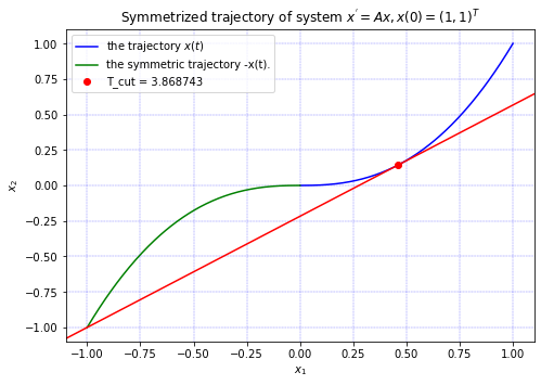
Figure 1:

Example 2

For the matrix $A=\left(\begin{array}[]{cc}-0.1&-0.3\\ 0.3&-0.1\end{array}\right)$, we have $\lambda_{1,2}\,=\,\alpha\pm\beta i=-0.1\pm 0.3i$. The space of quasipolynomials is $\mathcal{P}_{A}=\textrm{Lin}\{e^{-0.1t}\sin(0.3t),e^{-0.1t}\cos(0.3t)\}$. Algorithm 1 produces the value $T_{cut}=5.9952163$. The value of $T_{cut}$ found by solving the equation (4) is $5.990737$, see fig. 2

Figure 2:

Example 3

For the ${4\times 4}$ matrix $A\,=\,\left(\begin{array}[]{cccc}4.8&7.5&16&12\\ -3&-4.7&-9.6&-7.2\\ -3.2&-4.8&-5.4&-3.6\\ 4&6&6&3.9\\ \end{array}\right),$ we have $\lambda_{1}=-0.1;\lambda_{2}=-0.2;\lambda_{2}=-0.5;\lambda_{2}=-0.6$. The corresponding space of quasipolynomials is $\mathcal{P}_{A}=\textrm{Lin}\{e^{-0.1t},e^{-0.2t},e^{-0.5t},e^{-0.6t}\}$. Algotithm 1 finds $T_{cut}=17.75795$. Thus, if the matrix $A$ presents in the linear switching systems, then the stability analysis can be done only for switching laws with the intervals of the regime $A$ shorter than $\,17.75795$.

Example 4

For the ${4\times 4}$ matrix $A\,=\,\left(\begin{array}[]{cccc}22.8&15.7&-74.5&-41.9\\ -11.6&-8.6&35.8&20.4\\ -1.2&-0.3&5.8&3\\ 10.2&5.7&-41.4&-21.2\\ \end{array}\right),$ the spectrum is $\alpha_{1}\pm\beta_{1}i=-0.1\pm 0.7;\alpha_{2}\pm\beta_{2}i=-0.5\pm 0.3i$. The corresponding space is $\mathcal{P}_{A}=\textrm{Lin}\{e^{-0.1t}\sin(0.7t),e^{-0.1t}\cos(0.7t),e^{-0.5t}\sin(0.3t)$,
$e^{-0.5t}\cos(0.3t)\}$. Applying algorithm 1 we get $T_{cut}=8.94363$. Thus, for linear switching systems that include this matrix, all the corresponding switching intervals can be chosen smaller than $8.94363$

Example 5

For the matrix $\left(\begin{array}[]{cccc}-1.24&-0.29&-0.58&-0.69\\ -0.765&-1.515&-1.105&-0.415\\ 1.31&1.66&0.37&0.86\\ 0.635&-0.315&0.695&0.185\\ \end{array}\right),$ the spectrum is $\lambda_{1,2}=-0.3;\alpha_{1}\pm\beta_{1}i=-0.8\pm 0.9i$. We have $T_{cut}=7.09526$.

Acknowledgements. The work of Vladimir Yu.Protasov was supported by the Russian Science Foundation under grant 20-11-20169 and was performed in Steklov Mathematical Institute of Russian Academy of Sciences.

References

- [1] N. E. Barabanov, Lyapunov indicator for discrete inclusions, I–III, Autom. Remote Control, 49 (1988), No 2, 152–157.
- [2] F. Blanchini, D, Casagrande and S. Miani, Modal and transition dwell time computation in switching systems: a set-theoretic approach, Automatica J. IFAC, 46(9):1477–1482, 2010.
- [3] F. Blanchini, S. Miani, A new class of universal Lyapunov functions for the control of uncertain linear systems, IEEE Trans. Automat. Control, 44 (1999), no 3, 641–647.
- [4] G. Chesi, P. Colaneri, J. C. Geromel, R. Middleton, and R. Shorten. A nonconservative LMI condition for stability of switched systems with guaranteed dwell time, IEEE Trans. Automat. Control, 57(5):1297–1302, 2012.
- [5] Y. Chitour, N. Guglielmi, V.Yu. Protasov, M. Sigalotti, Switching systems with dwell time: computing the maximal Lyapunov exponent, Nonlinear Anal. Hybrid Syst. 40 (2021), Paper No. 101021, 21 pp.
- [6] V.K. Dzyadyk and I.A. Shevchuk, Theory of uniform approximation of functions by polynomials, Walter de Gruyter, 2008.
- [7] J. C. Geromel and P. Colaneri. Stability and stabilization of continuous-time switched linear systems, SIAM J. Control Optim., 45(5):1915–1930, 2006.
- [8] N. Guglielmi, L. Laglia, and V. Protasov. Polytope Lyapunov functions for stable and for stabilizable LSS, Found. Comput. Math., 17(2):567–623, 2017.
- [9] B. Ingalls, E. Sontag, and Y. Wang. An infinite-time relaxation theorem for differential inclusions, Proceedings of the American Mathematical Society, 131(2):487–499, 2003.
- [10] S. Karlin and W.J. Studden, Tchebycheff Systems: With Applications in Analysis and Statistics, Interscience, New York, 1966
- [11] G.G. Magaril-Ilyaev, V.M.,Tikhomirov, Convex Analysis: Theory and Applications (Translations of Mathematical Monographs) Amer. Mathematical Society (2003).
- [12] D. Liberzon. Switching in systems and control. Systems & Control: Foundations & Applications. Birkhäuser Boston, Inc., Boston, MA, 2003.
- [13] T. Mejstrik. Improved invariant polytope algorithm and applications, ACM Trans. Math. Softw., ACM Transactions on Mathematical Software 46 (2020), no 3, p. 1–26, https://doi.org/10.1145/3408891.
- [14] A. P. Molchanov and E. S. Pyatnitskiĭ. Lyapunov functions that define necessary and sufficient conditions for absolute stability of nonlinear nonstationary control systems. III Avtomat. i Telemekh. (5):38–49, 1986.
- [15] A. P. Molchanov and Y. S. Pyatnitskiy. Criteria of asymptotic stability of differential and difference inclusions encountered in control theory, Systems Control Lett., 13(1):59–64, 1989.
- [16] V.I. Opoitsev, Equilibrium and stability in models of collective behaviour, Nauka, Moscow (1977).
- [17] V.Yu. Protasov, The Barabanov norm is generically unique, simple, and easily computed SIAM J. Cont. Opt. 60 (2022), no 4.
- [18] V.Yu. Protasov, R. Kamalov, Stability of linear systems with bounded switching intervals, arXiv:2205.15446
- [19] E.Ya. Remez, Sur le calcul effectiv des polynomes d’approximation des Tschebyscheff, Compt. Rend. Acade. Sc. 199, 337 (1934).
- [20] M. Souza, A. Fioravanti, and R. Shorten. Dwell-time control of continuous-time switched linear systems. In Proceedings of the 54th IEEE Conference on Decision and Control, pages 4661–4666, 2015.
- [21] A. van der Schaft and H. Schumacher. An introduction to hybrid dynamical systems, volume 251 of Lecture Notes in Control and Information Sciences. Springer-Verlag London, Ltd., London, 2000.