Capacity dependent analysis for functional online learning algorithms

Abstract

This article provides convergence analysis of online stochastic gradient descent algorithms for functional linear models. Adopting the characterizations of the slope function regularity, the kernel space capacity, and the capacity of the sampling process covariance operator, significant improvement on the convergence rates is achieved. Both prediction problems and estimation problems are studied, where we show that capacity assumption can alleviate the saturation of the convergence rate as the regularity of the target function increases. We show that with properly selected kernel, capacity assumptions can fully compensate for the regularity assumptions for prediction problems (but not for estimation problems). This demonstrates the significant difference between the prediction problems and the estimation problems in functional data analysis.

Key words and phrases: Functional data analysis, Stochastic gradient decent, Reproducing kernel Hilbert space, Capacity dependent analysis

1 Introduction

In this paper, we consider a functional linear model

$$Y=\int_{\mathcal{T}}\beta^{*}(u)X(u)du+\varepsilon.$$ (1.1)

Here, $\mathcal{T}$ is a compact subset in a Euclidean space $\mathbb{R}^{d}$, $X$ is a random function, $\beta^{*}$ is an unknown slope function, $\varepsilon$ is a centered random noise with finite variance $\sigma^{2}=\mathrm{Var}(\varepsilon)<\infty$, and $Y\in\mathbb{R}$ is the response. We write $(L^{2}(\mathcal{T}),\left<\cdot,\cdot\right>_{2},\left\|\cdot\right\|_{2})$ the space of square integrable functions on $\mathcal{T}$, and assume $X,\beta^{*}\in L^{2}(\mathcal{T})$. Then, Model (1.1) can be equivalently written as $Y=\left<\beta^{*},X\right>_{2}+\varepsilon$. Without loss of generality, we assume that $\mathcal{T}=[0,1]^{d}$ throughout the paper.

We study two kinds of learning problems for Model (1.1). The estimation problem asks one to recover the unknown slope function $\beta^{*}$, and the prediction problem asks one to recover the linear functional on $L^{2}(\mathcal{T})$, denoted by $\varphi^{*}$, which is given by

$$\varphi^{*}:f\mapsto\left<\beta^{*},f\right>_{2}=\int_{\mathcal{T}}\beta^{*}(u)f(u)du.$$ (1.2)

Mathematically, $\varphi^{*}$ is defined with $\beta^{*}$, which in turn is fully determined by $\varphi^{*}$ through the Riesz representation theorem. Nonetheless, it is well understood that the two learning problems are different. In particular, the integral in (1.2) brings a smoothing effect, leading to a weaker regularity requirement for the prediction problems [4, 7].

Write $D=\{(x_{t},y_{t})\}_{t=1}^{T}$ a sample of independent copies of $(X,Y)$ in Model (1.1). We study both the case of a finite sample $T<\infty$, and the case $T=\infty$ where $D$ models an ongoing indefinite sampling process.

Both prediction and estimation problems can be solved by constructing an estimator $\hat{\beta}$ of the slope function $\beta^{*}$. In the literature, many works have been done on functional principal component analysis (FPCA) [19, 4, 15]. FPCA defines $\hat{\beta}$ with a linear combination of the estimated eigenfunctions of $C$, which is the covariance function of the random function $X$. Another approach of constructing $\hat{\beta}$ is the kernel method, which adopts a reproducing kernel $K$ and represents $\hat{\beta}$ by the linear combination of kernel functions [23, 5].

We adopt the kernel method and define $\hat{\beta}$ through stochastic gradient descent approach in this paper. A reproducing kernel $K$ on $\mathcal{T}$ is defined as a function $K:\mathcal{T}\times\mathcal{T}\to\mathbb{R}$ that is symmetric (i.e. $K(u,v)=K(v,u)$ for any $u,v\in\mathcal{T}$) and positive semi-definite (which requires that the Gram matrix $(K(u_{i},u_{j}))_{i,j=1}^{n}$ is positive semi-definite for any $n\geq 1$ and any $u_{1},\ldots,u_{n}\in\mathcal{T}$). We further assume that $K$ is continuous, exclude the trivial case $K\equiv 0$, and let $(\mathcal{H}_{K},\left<\cdot,\cdot\right>_{K},\left\|\cdot\right\|_{K})$ denote the reproducing kernel Hilbert space (RKHS) associated with $K$ [8, 20]. The stochastic gradient descent algorithm defines a sequence $\{\hat{\beta}_{t}\}$ of estimators, from $\hat{\beta}_{1}=0$ and then iteratively by

$$\hat{\beta}_{t+1}=\hat{\beta}_{t}-\eta_{t}\left(\int_{\mathcal{T}}\hat{\beta}_{t}(u)x_{t}(u)du-y_{t}\right)\int_{\mathcal{T}}K(v,\cdot)x_{t}(v)dv,\quad\mbox{for }t\geq 1.$$ (1.3)

Here $\eta_{t}>0$ is the step-size. Based on the nature of the sample $D$, we study two settings of the step-sizes $\{\eta_{t}\}$.

• The online setting. We write $|D|=\infty$ and use $D$ to model the outcome of an ongoing and indefinite sampling process. The estimator $\hat{\beta}$ is being updated following the sampling process. For example, we update the estimator to $\hat{\beta}=\hat{\beta}_{t+1}$ after $t$ steps of iterations and before the observation $(x_{t+1},y_{t+1})$ is available. For the online setting, the step-sizes $\{\eta_{t}\}$ are designed to decrease, rendering Algorithm (1.3) more and more conservative against the possible random noise brought by new observations.

• The finite-horizon setting. We assume a finite sample $D$ with size $|D|=T<\infty$. A constant step-size $\eta_{t}\equiv\eta=\eta(T)$ is adopted throughout the iterations (1.3) with $t=1,\ldots,T$. The sample $D$ is then exhausted and we use $\hat{\beta}=\hat{\beta}_{T+1}$ as the derived estimator. The step-size $\eta(T)$ can be optimized (at least asymptotically) over $T$, but it could be not trivial later to warm-start the iteration efficiently when new sample points are available.

To measure the estimation performance of $\hat{\beta}$, we use the expected squared $\mathcal{H}_{K}$ norm $\mathbb{E}[\|\hat{\beta}-\beta^{*}\|^{2}_{K}]$. Write $\hat{\varphi}:L^{2}(\mathcal{T})\to L^{2}(\mathcal{T})$ the estimator of the functional $\varphi^{*}$,

$$\hat{\varphi}:f\mapsto\langle\hat{\beta},f\rangle_{2}=\int_{\mathcal{T}}\hat{\beta}(u)f(u)du.$$

The prediction performance of $\hat{\varphi}$ is measured by the expected excess generalization error $\mathbb{E}[\mathcal{E}(\hat{\varphi})]$. Here for any linear functional $\varphi$ on $L^{2}(\mathcal{T})$,

$$\mathcal{E}(\varphi)=\mathbb{E}[(Y-\varphi(X))^{2}-(Y-\varphi^{*}(X))^{2}],$$

where the expectation is taken with respect to the distribution of $(X,Y)$ in Model (1.1).

As a technical instrument, the integral operator $L_{K}:L^{2}(\mathcal{T})\to L^{2}(\mathcal{T})$ is defined with the reproducing kernel $K$, by

$$L_{K}(f)=\int_{\mathcal{T}}K(\cdot,u)f(u)du.$$ (1.4)

It is well understood in the literature that $L_{K}$ is positive semi-definite (thus self-adjoint), and of trace class (so, compact). See, e.g., [20, Theorem 4.27]. The power $L_{K}^{r}$ with $r\in(0,\infty)$ is well defined by the spectral theorem. In terms of $L_{K}$, the iteration (1.3) is equivalently written as

$$\hat{\beta}_{t+1}=\hat{\beta}_{t}-\eta_{t}\left(\langle\hat{\beta}_{t},x_{t}\rangle_{2}-y_{t}\right)L_{K}x_{t},\quad\mbox{for }t\geq 1.$$ (1.5)

For the sake of simplicity we assume $\mathbb{E}[X]=0$ and $\|X\|_{2}=1$ a.s. Consequently, $\mathbb{E}[Y]=0$. The covariance function $C$ has the form

$$C(u,v)=\mathbb{E}[X(u)X(v)],\quad\mbox{for }u,v\in\mathcal{T}.$$

Obviously $C$ is also a reproducing kernel. We further assume that $C$ is continuous, exclude the trivial case $C\equiv 0$, and define the operator $L_{C}$ on $L^{2}(\mathcal{T})$ in the same way as (1.4) by substituting $K$ with $C$. So, $L_{C}$ is self-adjoint, positive semi-definite, of trace class, and thus compact. The power $L_{C}^{r}$ with $r>0$ is well defined. For any $f,g,h\in L^{2}(\mathcal{T})$, we define $f\otimes g$ as a rank-one operator on $L^{2}(\mathcal{T})$ defined by $(f\otimes g)h=\left<g,h\right>_{2}f$. For any linear functional $\varphi(\cdot)=\left<\beta,\cdot\right>_{2}$ on $L^{2}(\mathcal{T})$, the excess generalization error can be written in terms of the norm of $L^{2}(\mathcal{T})$,

$$\mathcal{E}(\varphi) =\mathbb{E}\left[(Y-\langle\beta,X\rangle_{2})^{2}-(Y-\langle\beta^{*},X\rangle_{2})^{2}\right]$$

$$=\mathbb{E}\left[\langle\beta-\beta^{*},X\rangle_{2}^{2}\right]=\mathbb{E}[\langle\beta-\beta^{*},X\otimes X(\beta-\beta^{*})\rangle_{2}]$$

$$=\|L_{C}^{1/2}(\beta-\beta^{*})\|^{2}_{2}.$$ (1.6)

Since $\mathcal{T}$ is compact, we write

$$\kappa=\max_{u\in\mathcal{T}}\sqrt{K(u,u)}\in(0,\infty).$$

Recall that by the positive semi-definiteness, $|K(u,v)|\leq\sqrt{K(u,u)K(v,v)}\leq\kappa^{2}$ for any $u,v\in\mathcal{T}$. The spectral norm of $L_{K}$ is bounded by $\|L_{K}\|_{\mathsf{op}(L^{2})}\leq\kappa^{2}$.

Modern scalable computing and stochastic optimization techniques make stochastic gradient descent a popular approach across various applications. Theoretical analysis of its convergence is also the subject of an intense recent study. The present work aims to establish a novel capacity-dependent convergence analysis for stochastic gradient descent (1.3) which is applied to solve the linear functional model (1.1) in an RKHS. We study prediction problem through the convergence of excess generalization error (1.6) and estimation problem through the strong convergence in an RKHS. Our analysis developed in this paper leads to fast rates for both types of convergence. State-of-the-art convergence rates in RKHS metric are obtained. From the viewpoint of approximation, this kind of convergence is much stronger, which ensures that the estimators can approximate the underlying target itself and its derivatives as well [24]. Our error estimates fully exploit the spectral structure of the operators and the capacity condition encoding the smoothness of kernels and covariance function. Our work provides insights for the applications of kernel methods to functional data analysis, and better understanding of the difference between the estimation problems and the prediction problems in functional linear models.

The rest of this paper will be organized as follows. We present the main results in Section 2. Discussions and comparisons with related works are given in Section 3. Section 4 introduces two novel error decomposition formulas of the algorithm (1.3). The proofs of main results are postponed to Section 5 and Section 6 after some preliminary estimates established for the convergence analysis.

2 Main Results

In this section we list some main assumptions and present the convergence rates of the stochastic gradient descent algorithm (1.3), in the finite-horizon and online settings, respectively. We provide discussions of the assumptions in Section 3.

Denote $\mathscr{L}_{K}=L_{C}^{1/2}L_{K}L_{C}^{1/2}$ and $\mathscr{L}_{C}=L_{K}^{1/2}L_{C}L_{K}^{1/2}$. It is easy to verify that both of the operators $\mathscr{L}_{K}$ and $\mathscr{L}_{C}$ are self-adjoint, positive semi-definite, of trace class, and compact.

Assumption 1 (Regularity Condition of the slope $\beta^{*}$).

There exists some $g^{*}$ in $L^{2}(\mathcal{T})$ and $r\in(0,\infty)$ such that

$$L_{C}^{1/2}\beta^{*}=\mathscr{L}^{r}_{K}g^{*}.$$

For any positive semi-definite compact operator $L$, let $\mathrm{Tr}(L)$ denote the trace of $L$, i.e., the sum of all the positive eigenvalues (counting multiplicity) of $L$. In particular, $\mathrm{Tr}(L)<\infty$ if and only if $L$ is of trace class.

Assumption 2 (Capacity Condition).

$$\mathrm{Tr}(\mathscr{L}^{s}_{K})<\infty,\quad\mbox{for some }0<s\leq 1.$$

Note that since $\mathscr{L}_{K}$ is a trace-class operator, Assumption 2 with $s=1$ holds true automatically.

Assumption 3 (Moment Condition).

For Model (1.1), there exist constant $c_{\mathsf{M}}>0$ such that for any $f$ in $L^{2}(\mathcal{T})$,

$$\mathbb{E}[\left<X,f\right>_{2}^{4}]\leq c_{\mathsf{M}}\left(\mathbb{E}[\langle X,f\rangle_{2}^{2}]\right)^{2}.$$ (2.1)

2.1 Analysis of the Prediction Error

In this subsection, we study the estimator $\hat{\varphi}=\langle\hat{\beta},\cdot\rangle_{2}$ for the prediction problem and bound the expected excess generalization error.

Theorem 1.

In the online setting, define $\{\hat{\varphi}_{t}=\langle\hat{\beta}_{t},\cdot\rangle_{2}\}$ through (1.3). Under Assumptions 1 (with $r>0$), 2 (with $0<s\leq 1$), and 3, set $\eta_{t}=\eta_{0}t^{-\theta}$ with

$$\theta=\frac{\min\{2r,2-s\}}{1+\min\{2r,2-s\}}=\left\{\begin{array}[]{ll}\frac{2r}{2r+1},&\mbox{when }2r\leq 2-s,\\ \frac{2-s}{3-s},&\mbox{when }2r\geq 2-s.\end{array}\right.$$ (2.4)

If $0<\eta_{0}\leq\min\{1,\kappa^{-2},C^{\mathsf{S}}_{1}\}$ (where $C^{\mathsf{S}}_{1}$ is a constant, and it will be specified by (5.24) in the proof), then

$$\mathbb{E}[\mathcal{E}(\hat{\varphi}_{t+1})]\leq C_{1}\left\{\begin{array}[]{ll}(t+1)^{-\theta},&0<s<1,\\ (t+1)^{-\theta}\log(t+1),&s=1,\end{array}\right.\quad\mbox{for any }t\geq 1,$$ (2.7)

where $C_{1}$ is a constant independent of $t$, and it will be specified by (5.26) in the proof.

For the piecewise definition (2.4), we let the domains overlap on purpose to highlight the continuity of $\theta$ on the whole domain $r>0$ and $0<s<1$. The index $\theta$ as a function of $r$ and $s$ is also visualized in Figure 1. Without Assumption 2 (i.e., case $s=1$ in (2.7)), the convergence rate $O((t+1)^{-2r/(2r+1)}\log(t+1))$, saturated as $O((t+1)^{-1/2}\log(t+1))$ for $r\geq 1/2$, is also obtained in [7]. Here, $r$ indicates the regularity of the target function $\beta^{*}$ as described in Assumption 1. The saturation means beyond $r\in(0,1/2]$, further improvement of such regularity (i.e., increasing of $r$) does not help to improve the rate $\mathbb{E}[\mathcal{E}(\hat{\varphi}_{t+1})]$ converges to zero. In this paper, Theorem 1 suggests that Assumption 2 on capacity with $s<1$, not only removes the logarithmic factor in the convergence rates, but also uplifts the saturating boundary from $1/2$ to $1/2+(1-s)/2$.

Figure 1: The index $\theta$ in Theorem 1 as a function of $(r,s)$. Here the double-headed arrows show the gradient directions.

In the following, Theorem 2 shows that in the finite-horizon setting, Algorithm (1.3) does not suffer from the above discussed saturation, and the expected prediction error converges to zero in a rate arbitrarily close to $O(T^{-1})$, for sufficiently large $r$.

Theorem 2.

In the finite-horizon setting with $1\leq T=|D|<\infty$, define $\hat{\varphi}_{T+1}=\langle\hat{\beta}_{T+1},\cdot\rangle_{2}$ through (1.3). Under Assumptions 1 (with $r>0$), 2 (with $0<s\leq 1$), and 3, set the constant step-size $\eta_{t}=\eta_{0}T^{-2r/(2r+1)}$, with $0<\eta_{0}\leq\min\{1,\kappa^{-2},C_{2}^{\mathsf{S}}\}$ (where $C_{2}^{\mathsf{S}}$ is a constant independent of $T$, and it will be specified by (5.31) in the proof). Then,

$$\mathbb{E}[\mathcal{E}(\hat{\varphi}_{T+1})]\leq C_{2}\left\{\begin{array}[]{ll}T^{-2r/(2r+1)},&\mbox{when }0<s<1,\\ T^{-2r/(2r+1)}\log(T+1),&\mbox{when }s=1.\end{array}\right.$$ (2.10)

where the constant $C_{2}$ is independent of $T$, and it will be specified by (5.35) in the proof.

The capacity independent convergence rate $O(T^{-2r/(2r+1)}\log(T+1))$ for $s=1$ in (2.10) is first derived in [7]. In the finite-horizon setting, the capacity assumption $0<s<1$ helps remove the logarithmic factor.

2.2 Analysis of the Estimation Error

In this subsection, we study the estimator $\hat{\beta}$ for the estimation problem. The analysis employs the following Assumption 4 to replace Assumption 1.

Assumption 4 (Regularity Condition of the slope $\beta^{*}$).

There exists some $g^{\dagger}$ in $L^{2}(\mathcal{T})$ and $r>0$, such that

$$\beta^{*}=L_{K}^{1/2}\mathscr{L}_{C}^{r}g^{\dagger}.$$

This assumption implies that the slope $\beta^{*}$ lies in the range of $L^{1/2}_{K}$, i.e., $\beta^{*}\in\mathcal{H}_{K}$.

Theorem 3.

In the online setting, define $\{\hat{\beta}_{t}\}_{t\geq 1}$ through (1.3). Under Assumptions 2 (with $0<s<1$), 3, and 4 (with $r>0$), set step-sizes $\eta_{t}=\eta_{0}t^{-\theta}$ with $0<\eta_{0}\leq\min\{1,\kappa^{-2},C_{3}^{\mathsf{S}}\}$ (where $C_{3}^{\mathsf{S}}$ is a constant independent of $t$, and it will be specified by (6.5) in the proof), and

$$\theta=\left\{\begin{array}[]{ll}\frac{2r+s}{2r+s+1},&\mbox{when }2r\leq 1-s,\\ 1/2,&\mbox{when }2r\geq 1-s.\end{array}\right.$$ (2.13)

Then,

$$\mathbb{E}[\|\hat{\beta}_{t+1}-\beta^{*}\|_{K}^{2}]\leq C_{3}\left\{\begin{array}[]{ll}(t+1)^{-2r/(1+s+2r)},&2r<1-s,\\ (t+1)^{-(1-s)/2}\log(t+1),&2r\geq 1-s,\end{array}\right.\quad\mbox{for any }t\geq 1,$$ (2.16)

where $C_{3}$ is a constant independent of $t$, and it will be specified by (6.11) in the proof.

In the definition (2.13), $\theta$ is a continuous function of $r>0$ and $0<s<1$. So we purposely use two overlapping domains. The power index of the rates in (2.16) will be elucidated in Figure 2.

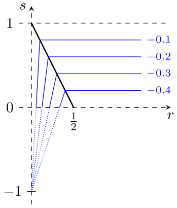
Figure 2: The power index $\tilde{\omega}(r,s)$ of the convergence estimate (2.16) in Theorem 3. The thick black line marks the boundary $2r=1-s$ of the two regimes. $\tilde{\omega}=-2r/(1+s+2r)$ when $2r\leq 1-s$, and $\tilde{\omega}=-(1-s)/2$ when $2r\geq 1-s$. Contours of $\tilde{\omega}$ are plotted in solid blue lines, and further extended by dotted lines.

Remark 1.

Theorem 3 does not work in the capacity independent setting $s=1$, where the convergence analysis remains an open problem.

Next we establish unsaturated convergence rates of estimation error for the finite-horizon setting.

Theorem 4.

In the finite-horizon setting with $1\leq T=|D|<\infty$, define $\{\hat{\beta}_{t}:1\leq t\leq T+1\}$ through (1.3). Under Assumptions 2 (with $0<s\leq 1$), 3, and 4 (with $r>0$), set the constant step-size $\eta_{t}=\eta_{0}T^{-(s+2r)/(1+s+2r)}$, with $0<\eta_{0}\leq\min\{1,\kappa^{-2},C_{4}^{\mathsf{S}}\}$ (where $C_{4}^{\mathsf{S}}$ is a constant independent of $T$, and it will be specified by (6.12) in the proof). Then,

$$\mathbb{E}[\|\hat{\beta}_{T+1}-\beta^{*}\|_{K}^{2}]\leq C_{4}T^{-2r/(1+s+2r)},$$ (2.17)

where the constant $C_{4}$ is independent of $T$, and it will be specified by (6.16) in the proof.

The rates (2.17) in Theorem 4 does not saturate for $r>0$, and are arbitrarily close to $O(T^{-1})$ for sufficiently large $r$. For a fixed $r>0$, with a smaller $s$ one has a faster rate in (2.17). Here, a smaller $s$ indicates a stronger capacity assumption (Assumption 2). As we shall see in Theorem 5 below, a smaller $s$ corresponds to faster eigenvalue decay for $\mathscr{L}_{K}$ (equivalently, faster eigenvalue decay for $\mathscr{L}_{C}$), and a smaller hypothesis space $L_{K}^{1/2}\mathscr{L}_{C}^{r}(L^{2}(\mathcal{T}))$ in Assumption 4.

3 Comparisons and Discussions

There has been rapidly growing literature focusing on stochastic gradient descent and its variants in an RKHS or general Hilbert spaces [22, 9, 18, 13, 2, 11]. We refer the readers to these papers and references therein. Our paper contributes to the theoretical analysis of functional linear regression in an RKHS that stems from the the work of Yuan and Cai which establishes capacity dependent analysis for batch learning [23, 5]. As far as we know, the convergence of stochastic gradient descent has not been investigated in the context of functional linear regression in an RKHS till the very recent paper [7] in which the authors conduct capacity independent analysis of the prediction error.

Under the batch leaning setting, Yuan and Cai [23] derive the minimax optimal convergence rate $T^{-2s_{*}/(2s_{*}+1)}$ of the excess generalization error $\mathcal{E}(\hat{\varphi}_{T+1})$ for prediction, with the regularity assumption $\beta^{*}\in\mathcal{H}_{K}$ and capacity assumption on the rates of eigenvalue decay, $\lambda_{i}(L_{K})\sim i^{-2s_{1}}$ (here $a_{i}\sim b_{i}$ means $a_{i}/b_{i}$ being uniformly bounded away from zero and infinity as $i\to\infty$) and $\lambda_{i}(L_{C})\sim i^{-2s_{2}}$, where $s_{1},s_{2}>1/2$ and $s_{*}=s_{1}+s_{2}$. Later, Cai and Yuan [5] derive the same rate with a different capacity assumption $\lambda_{i}(\mathscr{L}_{C})\sim i^{-2s_{*}}$.

Compared with these works, the strength of our analysis includes that first, our Assumption 2 on capacity, $\mathrm{Tr}(\mathscr{L}_{K}^{s})<\infty$, is way more general. We shall see in Theorem 5 that this is roughly equivalent to the assumption $\lambda_{i}(\mathscr{L}_{K})=O(i^{-1/s})$. We shall see in Remark 3 that although the eigenvalues $\{\lambda_{i}(\mathscr{L}_{K})\}_{i=1}^{\infty}$ are arranged non-increasingly, in general there is no exact index $s_{*}$ such that $\lambda_{i}(\mathscr{L}_{K})\sim i^{-2s_{*}}$ (same for other compact operators including $L_{K}$, $L_{C}$, and $\mathscr{L}_{C}$). Second, our analysis supports finer characterizations $L_{C}^{1/2}\beta^{*}=\mathscr{L}_{K}^{r}(g^{*})$ (Assumption 1) and $\beta^{*}=L_{K}^{1/2}\mathscr{L}_{C}^{r}(g^{\dagger})$ (Assumption 4) of slope function regularity. This leads to a better convergence rate $O(T^{-2r/(2r+1)})$ in Theorem 2, than $O(T^{-2s_{*}/(2s_{*}+1)})$ when $r>s_{*}$. Third, we proved the non-trivial convergence rates for the estimation error $\|\hat{\beta}-\beta^{*}\|_{K}^{2}$ in $\mathcal{H}_{K}$ metric, $O(T^{-2r/(2r+1)})$ (saturated at $r=(1-s)/2$) in the online setting in Theorem 3, and $O(T^{-2r/(1+s+2r)})$ in the finite-horizon setting in Theorem 4. Note that the analysis in [23] just provides a constant rate $O(1)$ for $\|\hat{\beta}-\beta^{*}\|_{K}^{2}$.

Next we provide some comments on the main assumptions in Section 2. For any bounded self-adjoint operators $A$ and $B$ on $L^{2}(\mathcal{T})$, we write $A\succeq B$ (or $B\preceq A$) if $A-B$ is positive semi-definite.

Remark 2.

It is well understood [7, Remark 1] that when $0<r<1/2$, if $L_{K}^{\tau}\succeq\delta L_{C}^{\nu}$ for some $\tau,\delta,\nu>0$ with $\tau+\nu\geq 1$ and $r=\tau/(2\tau+2\nu)$, then Assumption 1 is guaranteed by any $\beta^{*}\in L^{2}(\mathcal{T})$. That is, with a carefully selected reproducing kernel $K$, for the prediction error to converge, the capacity assumption (Assumption 2) can fully compensate for the regularity assumption (Assumption 1). Note that the above condition $L_{K}^{\tau}\succeq\delta L_{C}^{\nu}$ puts some requirement on the selection of the reproducing kernel $K$, but it does not require the one-to-one matching between the eigenfunctions of $L_{K}$ and $L_{C}$, respectively.

Similarly, if $L_{C}\succeq\delta L_{K}^{\nu}$ for some $\delta,\nu>0$, then Assumption 4 with $0<r\leq 1/2$ is guaranteed when $\beta^{*}\in L_{K}^{r(1+\nu)+\frac{1}{2}}(L^{2}(\mathcal{T}))$. However, Assumption 4 implies $\beta^{*}\in L_{K}^{1/2}(L^{2}(\mathcal{T}))$. Therefore, the regularity assumption for the estimation error to converge, can not be fully compensated for by the capacity assumption. This demonstrates a significant difference between the prediction problems, and the estimation problems in functional data analysis.

In the literature of kernel-based learning algorithms [6, 1, 3, 17, 14, 12, 21, 16], the capacity of the hypothesis space $\mathcal{H}_{K}$ is usually measured by covering numbers, or the effective dimension $\mathcal{N}_{L_{K}}(\lambda)=\mathrm{Tr}((L_{K}+\lambda I)^{-1}L_{K})$, where $I$ denotes the identity operator. A typical capacity assumption takes the form $\mathcal{N}_{L_{K}}(\lambda)=O(\lambda^{-s})$ (as $\lambda\downarrow 0$) for some $0<s<1$, and is well understood. The following theorem shows that roughly speaking, Assumption 2 with $0<s<1$ is comparable to the assumption $\mathcal{N}_{\mathscr{L}_{K}}(\lambda)=O(\lambda^{-s})$ as $\lambda\downarrow 0$. The conclusion is well understood [13, 11], but the proof through (3.1), is to our best knowledge not available elsewhere.

Theorem 5.

Let $L$ be a positive semi-definite operator of trace class with infinite positive eigenvalues $\{\lambda_{i}=\lambda_{i}(L)\}_{i=1}^{\infty}$ arranged in non-increasing order. Let $0<s<1$. We have

$$\mathrm{Tr}(L^{s})=\frac{\sin(\pi s)}{\pi}\int^{\infty}_{0}\lambda^{s-1}\mathcal{N}_{L}(\lambda)d\lambda.$$ (3.1)

Consequently,

• If $\mathrm{Tr}(L^{s})<\infty$, then $\mathcal{N}_{L}(\lambda)=O(\lambda^{-s})$ as $\lambda\downarrow 0$;

• If $\mathcal{N}_{L}(\lambda)=O(\lambda^{-s})$ as $\lambda\downarrow 0$, then $\mathrm{Tr}(L^{s+\epsilon})<\infty$ for any $\epsilon>0$;

• Moreover, for any fixed $0<s<1$, $\mathcal{N}_{L}(\lambda)=O(\lambda^{-s})$ as $\lambda\downarrow 0$ if and only if $\lambda_{i}=O(i^{-1/s})$ as $i\to\infty$.

The relations listed in Theorem 5 are summarized in Figure 3.

Figure 3: Summary of the relations listed in Theorem 5.

The case $L$ has only finite positive eigenvalue is trivial, where $\mathcal{N}_{L}(\lambda)=O(1)$ as $\lambda\downarrow 0$ and $\mathrm{Tr}(L^{s})<0$ for any $s>0$.

Note that on the one hand, when $L^{s}$ does not belong to the trace class (equivalently, $\mathrm{Tr}(L^{s})=\infty$), Equation (3.1) implies that the integral on its right-hand side diverges to infinity. On the other hand, when this integral diverges to infinity, $\mathrm{Tr}(L^{s})=\infty$.

The bound $\mathcal{N}_{L}(\lambda)=O(\lambda^{-s})$ as $\lambda\downarrow 0$ does not guarantee $\mathrm{Tr}(L^{s})<\infty$. For example, $\lambda_{i}=i^{-1/s}$ implies $\mathrm{Tr}(L^{s})=\infty$, yet we still have

$$\mathcal{N}_{L}(\lambda)=\sum^{\infty}_{i=1}\frac{1}{1+\lambda i^{1/s}}\leq\int^{\infty}_{0}\frac{du}{1+\lambda u^{1/s}}=\lambda^{-s}\int^{\infty}_{0}\frac{du}{1+u^{1/s}}=O(\lambda^{-s}),\quad\mbox{as }\lambda\downarrow 0.$$

Remark 3.

Note that in general, for a non-increasing sequence $\{a_{i}\}_{k=1}^{\infty}\subset(0,\infty)$, Theorem 5 does not suggest the existence of some $\gamma>0$ such that $a_{k}\sim k^{-\gamma}$. It is easy to construct a non-increasing sequence that stays between $k^{-\gamma_{1}}$ and $k^{-\gamma_{2}}$ for any $\gamma_{1}>\gamma_{2}>0$. To this end, we define $\{b_{k}\}$ as $b_{1}=2$ and $b_{k+1}=b_{k}^{\gamma_{1}/\gamma_{2}}$ for $k\geq 1$. We define a function $f$ on $[2,\infty)$, piece-wisely by $f(x)=b_{k}^{-\gamma_{1}}$ for $b_{k}\leq x<b_{k+1}$. Writing $a_{k}=f(k+1)$ to give

$$\limsup_{k\to\infty}\frac{a_{k}}{k^{-\gamma_{2}}}=\liminf_{k\to\infty}\frac{a_{k}}{k^{-\gamma_{1}}}=1.$$

Proof of Theorem 5.

Write $B(u,v)$ the Euler beta function for $u,v>0$. Recall that for any $a>0$,

$$\frac{\pi}{\sin(\pi s)}=B(s,1-s)=\int^{\infty}_{0}\frac{\xi^{s-1}}{1+\xi}d\xi\overset{\xi=\lambda/a}{=\!=\!=\!=}a^{-s}\int^{\infty}_{0}\frac{a\lambda^{s-1}}{a+\lambda}d\lambda.$$

So,

$$a^{s}=\frac{\sin(\pi s)}{\pi}\int^{\infty}_{0}\lambda^{s-1}\frac{a}{a+\lambda}d\lambda.$$ (3.2)

In (3.2) substitute $a$ with all the positive eigenvalues of $L$ respectively, and take the sum to obtain (3.1). Since $L$ is of trace class, $\mathcal{N}_{L}(\lambda)$ is well defined for each $\lambda>0$. Obviously $\lambda^{s-1}$ and $\mathcal{N}_{L}(\lambda)$ are non-increasing. So when $\mathrm{Tr}(L^{s})<\infty$,

$$\lambda^{s}\mathcal{N}_{L}(\lambda)=\lambda^{s-1}\mathcal{N}_{L}(\lambda)\int^{\lambda}_{0}d\xi<\int^{\infty}_{0}\xi^{s-1}\mathcal{N}_{L}(\xi)d\xi=\frac{\pi\mathrm{Tr}(L^{s})}{\sin(\pi s)}<\infty,$$

which verifies (a). Now assume $\mathcal{N}_{L}(\lambda)=O(\lambda^{-s})$ as $\lambda\downarrow 0$. Then there are two constants $0<\delta,C_{1}<\infty$ such that $0\leq\mathcal{N}_{L}(\lambda)\leq C_{1}\lambda^{-s}$ for any $0<\lambda\leq\delta$. So,

$$\int^{\delta}_{0}\lambda^{s+\epsilon-1}\mathcal{N}_{L}(\lambda)d\lambda\leq C_{1}\int^{\delta}_{0}\lambda^{\epsilon-1}d\lambda<\infty.$$

Since $L$ is in the trace class, when $s+\epsilon\geq 1$, (b) is trivial. Now we assume $s+\epsilon<1$. Note that $\mathcal{N}_{L}(\lambda)\leq\mathrm{Tr}(L)/\lambda$. So

$$\int^{\infty}_{\delta}\lambda^{s+\epsilon-1}\mathcal{N}_{L}(\lambda)d\lambda\leq\mathrm{Tr}(L)\int^{\infty}_{\delta}\lambda^{s+\epsilon-2}d\lambda<\infty.$$

The claim (b) is verified by combining the above two bounds together.

Now we verify item (c). When $\lambda_{i}=O(i^{-1/s})$, there is some constant $C_{2}>0$ such that $\lambda_{i}\leq C_{2}i^{-1/s}$ for all $i\geq 1$. Since $u/(u+\lambda)$ is an increasing function of $u$,

$$\mathcal{N}_{L}(\lambda)\leq\sum^{\infty}_{i=1}\frac{C_{2}i^{-1/s}}{C_{2}i^{-1/s}+\lambda}=\sum^{\infty}_{i=1}\frac{1}{1+\lambda i^{1/s}/C_{2}}$$

$$\leq\int^{\infty}_{0}\frac{du}{1+\lambda u^{1/s}/C_{2}}=\left(\frac{\lambda}{C_{2}}\right)^{-s}\int^{\infty}_{0}\frac{du}{1+u^{1/s}}=O(\lambda^{-s}).$$

This verifies the “if” part. For the “only-if” part, when $\mathcal{N}_{L}(\lambda)=O(\lambda^{-s})$, it is easy to see that there is some $C_{3}>0$ such that $\mathcal{N}_{L}(\lambda)\leq C_{3}\lambda^{-s}$ for every $0<\lambda\leq s\lambda_{1}/(1-s)$. Since for a fixed $\lambda$, $\{\lambda_{i}/(\lambda_{i}+\lambda)\}^{\infty}_{i=1}$ is a non-increasing sequence, $i\lambda_{i}/(\lambda_{i}+\lambda)\leq C_{3}\lambda^{-s}$ for each $\lambda\in(0,s\lambda_{1}/(1-s)]$ and $i\geq 1$. Therefore,

$$i\lambda_{i}\leq\inf_{\lambda\in(0,s\lambda_{1}/(1-s)]}C_{3}\lambda^{-s}(\lambda_{i}+\lambda)=C_{3}\lambda_{i}^{1-s}s^{s}(1-s)^{1-s},$$ (3.3)

where the infimum is achieved at $\lambda=s\lambda_{i}/(1-s)\in(0,s\lambda_{1}/(1-s)]$. From (3.3) one obtains $\lambda_{i}=O(i^{-1/s})$ as $i\to\infty$, and completes the proof. ∎

Assumption 3 is quite often adopted in the literature of functional linear regression. For example, if $X$ is a Gaussian process, then (2.1) is satisfied with $c_{\mathsf{M}}=3$. See [23, 5, 10].

4 Error Decomposition

Our analysis starts with error decomposition. By (1.5), i.e., the equivalent expression of algorithm (1.3), for any $t\geq 1$,

$$\hat{\beta}_{t+1}-\beta^{*} =\hat{\beta}_{t}-\beta^{*}-\eta_{t}(\langle\hat{\beta}_{t},x_{t}\rangle_{2}-y_{t})L_{K}x_{t}$$

$$=(I-\eta_{t}L_{K}L_{C})(\hat{\beta}_{t}-\beta^{*})+\mathcal{B}_{t},$$ (4.1)

where $\mathcal{B}_{t}=\eta_{t}(y_{t}-\langle\hat{\beta}_{t},x_{t}\rangle_{2})L_{K}x_{t}+\eta_{t}L_{K}L_{C}(\hat{\beta}_{t}-\beta^{*})$, of which the second term is the conditional mean of the first term,

$$\mathbb{E}_{z_{t}}\left[(y_{t}-\langle\hat{\beta}_{t},x_{t}\rangle_{2})L_{K}x_{t}\right] =\mathbb{E}_{x_{t}}\left[\langle\beta^{*}-\hat{\beta}_{t},x_{t}\rangle_{2}L_{K}x_{t}\right]$$

$$=L_{K}L_{C}(\beta^{*}-\hat{\beta}_{t}).$$ (4.2)

Where $z_{t}=(x_{t},y_{t})$, and the expectations $\mathbb{E}_{z_{t}}$ and $\mathbb{E}_{x_{t}}$ are taken with respect to the (conditional) distributions of $z_{t}=(x_{t},y_{t})$ and $x_{t}$, respectively. Equation (4.2) shows that $\mathcal{B}_{t}$ is mean-zero, $\mathbb{E}_{z_{t}}[\mathcal{B}_{t}]=0$. Then applying induction to (4.1) implies that for any $t\geq 1$,

$$\hat{\beta}_{t+1}-\beta^{*}=-\left[\prod_{k=1}^{t}(I-\eta_{k}L_{K}L_{C})\right]\beta^{*}+\sum_{k=1}^{t}\left[\prod_{j=k+1}^{t}(I-\eta_{j}L_{K}L_{C})\right]\mathcal{B}_{k},$$ (4.3)

where and in the following, the product of an empty set of operators is defined as the identity operator, $\prod_{j=t+1}^{t}(I-\eta_{j}L_{K}L_{C})=I$. Recall that $\mathscr{L}_{K}=L_{C}^{1/2}L_{K}L_{C}^{1/2}$.

Proposition 6.

Define $\{\hat{\varphi}_{t}=\langle\hat{\beta}_{t},\cdot\rangle_{2}:t\geq 1\}$ through (1.3). Then for any $t\geq 0$,

$$\mathbb{E}\left[\mathcal{E}(\hat{\varphi}_{t+1})\right]\leq\left\|\left[\prod^{t}_{k=1}(I-\eta_{k}\mathscr{L}_{K})\right]L_{C}^{1/2}\beta^{*}\right\|_{2}^{2}$$

$$+\sum^{t}_{k=1}\eta_{k}^{2}\left(\sigma^{2}+\mathbb{E}\sqrt{\mathbb{E}_{x_{k}}\langle\beta^{*}-\hat{\beta}_{k},x_{k}\rangle_{2}^{4}}\right)\left[\mathbb{E}\left\|\left[\prod^{t}_{j=k+1}(I-\eta_{j}\mathscr{L}_{K})\right]L_{C}^{1/2}L_{K}x_{k}\right\|_{2}^{4}\right]^{1/2},$$ (4.4)

where the sum of an empty set is defined as zero.

Proof.

The case $t=0$ is trivial and we assume $t\geq 1$. For any $k$,

$$L_{C}^{1/2}(I-\eta_{k}L_{K}L_{C})=L_{C}^{1/2}-\eta_{k}\mathscr{L}_{K}L_{C}^{1/2}=\left(I-\eta_{k}\mathscr{L}_{K}\right)L_{C}^{1/2}.$$

From (4.3),

$$L_{C}^{1/2}(\hat{\beta}_{t+1}-\beta^{*})=-\left[\prod_{k=1}^{t}\left(I-\eta_{k}\mathscr{L}_{K}\right)\right]L_{C}^{1/2}\beta^{*}+\sum_{k=1}^{t}\left[\prod_{j=k+1}^{t}\left(I-\eta_{j}\mathscr{L}_{K}\right)\right]L_{C}^{1/2}\mathcal{B}_{k}.$$

It follows from (1.6) that

$$\mathbb{E}\left[\mathcal{E}(\hat{\varphi}_{t+1})\right]=\mathbb{E}\left[\left\|L_{C}^{1/2}(\hat{\beta}_{t+1}-\beta^{*})\right\|_{2}^{2}\right]$$

$$= \mathbb{E}\left[\left\|-\left[\prod_{k=1}^{t}\left(I-\eta_{k}\mathscr{L}_{K}\right)\right]L_{C}^{1/2}\beta^{*}+\sum_{k=1}^{t}\left[\prod_{j=k+1}^{t}\left(I-\eta_{j}\mathscr{L}_{K}\right)\right]L_{C}^{1/2}\mathcal{B}_{k}\right\|_{2}^{2}\right]$$

$$= \left\|\left[\prod_{k=1}^{t}(I-\eta_{k}\mathscr{L}_{K})\right]L_{C}^{1/2}\beta^{*}\right\|_{2}^{2}+\mathbb{E}\left[\left\|\sum_{k=1}^{t}\left[\prod_{j=k+1}^{t}(I-\eta_{j}\mathscr{L}_{K})\right]L_{C}^{1/2}\mathcal{B}_{k}\right\|_{2}^{2}\right]$$

$$= :\Upsilon^{\mathsf{E}}_{1}+\Upsilon^{\mathsf{E}}_{2}$$ (4.5)

where in the expansion of the squared norm, the cross terms vanish because $\mathbb{E}[\mathcal{B}_{k}]=\mathbb{E}_{z_{k}}[\mathcal{B}_{k}]=0$. The notations $\Upsilon^{\mathsf{E}}_{1}$ and $\Upsilon^{\mathsf{E}}_{2}$ are used only within this proof. When $k\neq s$, without loss of generality assume $k>s$. Recall that then $\mathcal{B}_{s}$ is independent of $z_{t}$. So,

$$\mathbb{E}_{z_{k}}\left<\left[\prod^{t}_{j=k+1}(I-\eta_{j}\mathscr{L}_{K})\right]L_{C}^{1/2}\mathcal{B}_{k},\left[\prod^{t}_{j=s+1}(I-\eta_{j}\mathscr{L}_{K})\right]L_{C}^{1/2}\mathcal{B}_{s}\right>_{2}=0.$$

So we expand the squared norm in $\Upsilon^{\mathsf{E}}_{2}$,

$$\Upsilon^{\mathsf{E}}_{2} =\sum_{k=1}^{t}\mathbb{E}\left[\left\|\left[\prod_{j=k+1}^{t}(I-\eta_{j}\mathscr{L}_{K})\right]L_{C}^{1/2}\mathcal{B}_{k}\right\|_{2}^{2}\right]$$

$$\leq\sum_{k=1}^{t}\eta_{k}^{2}\mathbb{E}\left[\mathbb{E}_{\varepsilon_{k}}[(y_{k}-\langle\hat{\beta}_{k},x_{k}\rangle_{2})^{2}]\left\|\left[\prod_{j=k+1}^{t}(I-\eta_{j}\mathscr{L}_{K})\right]L_{C}^{1/2}L_{K}x_{k}\right\|_{2}^{2}\right],$$ (4.6)

where the inequality is obtained by recalling the zero-mean structure $\mathcal{B}_{t}=\eta_{t}(y_{t}-\langle\hat{\beta},x_{t}\rangle_{2})L_{K}x_{t}-\mathbb{E}_{x_{t}}[\eta_{t}(y_{t}-\langle\hat{\beta},x_{t}\rangle_{2})L_{K}x_{t}]$ explained in (4.2). Furthermore, we recall that $\mathbb{E}_{\varepsilon_{k}}[(y_{k}-\langle\hat{\beta}_{k},x_{k}\rangle_{2})^{2}]=\sigma^{2}+\langle\beta^{*}-\hat{\beta}_{k},x_{k}\rangle_{2}^{2}$ and obtain

$$\Upsilon^{\mathsf{E}}_{2}\leq\, \sigma^{2}\sum_{k=1}^{t}\eta_{k}^{2}\mathbb{E}\left[\left\|\left[\prod_{j=k+1}^{t}(I-\eta_{j}\mathscr{L}_{K})\right]L_{C}^{1/2}L_{K}x_{k}\right\|_{2}^{2}\right]$$

$$+\sum_{k=1}^{t}\eta_{k}^{2}\mathbb{E}\left[\langle\beta^{*}-\hat{\beta}_{k},x_{k}\rangle_{2}^{2}\left\|\left[\prod_{j=k+1}^{t}(I-\eta_{j}\mathscr{L}_{K})\right]L_{C}^{1/2}L_{K}x_{k}\right\|_{2}^{2}\right].$$ (4.7)

The proof is complete by applying Cauchy-Schwarz inequality to the right-hand side of (4.7). ∎

Now we consider the error decomposition for estimation error.

Proposition 7.

Let $\{\hat{\beta}_{t}\}$ be defined by (1.3). Assume $\beta^{*}\in\mathcal{H}_{K}$. We have the following error decomposition for any $t\geq 0$.

$$\mathbb{E} \left[\|\hat{\beta}_{t+1}-\beta^{*}\|_{K}^{2}\right]\leq\left\|\left[\prod_{k=1}^{t}(I-\eta_{k}L_{K}L_{C})\right]\beta^{*}\right\|_{K}^{2}$$

$$+\sum^{t}_{k=1}\eta_{k}^{2}\left(\sigma^{2}+\mathbb{E}\sqrt{\mathbb{E}_{x_{k}}\langle\beta^{*}-\hat{\beta}_{k},x_{k}\rangle_{2}^{4}}\right)\left(\mathbb{E}\left\|\left[\prod^{t}_{j=k+1}(I-\eta_{j}L_{K}L_{C})\right]L_{K}x_{k}\right\|_{K}^{4}\right)^{1/2}$$ (4.8)

Proof.

The proof parallels that of Proposition 6. By (4.3) and the fact $\mathbb{E}[\mathcal{B}_{k}]=0$ we have

$$\mathbb{E}\left[\|\hat{\beta}_{t+1}-\beta^{*}\|_{K}^{2}\right]=\mathbb{E}\left[\left\|-\left[\prod_{k=1}^{t}(I-\eta_{t}L_{K}L_{C})\right]\beta^{*}+\sum_{k=1}^{t}\left[\prod_{j=k+1}^{t}(I-\eta_{j}L_{K}L_{C})\right]\mathcal{B}_{k}\right\|_{K}^{2}\right]$$

$$=\left\|\left[\prod_{k=1}^{t}(I-\eta_{k}L_{K}L_{C})\right]\beta^{*}\right\|_{K}^{2}+\mathbb{E}\left[\left\|\sum_{k=1}^{t}\left[\prod_{j=k+1}^{t}(I-\eta_{j}L_{K}L_{C})\right]\mathcal{B}_{k}\right\|_{K}^{2}\right],$$ (4.9)

where the second term on the right-hand side is further estimated with the trick we used in (4.6).

$$\mathbb{E}\left[\left\|\sum_{k=1}^{t}\left[\prod_{j=k+1}^{t}(I-\eta_{j}L_{K}L_{C})\right]\mathcal{B}_{k}\right\|_{K}^{2}\right]=\sum_{k=1}^{t}\mathbb{E}\left[\left\|\left[\prod_{j=k+1}^{t}(I-\eta_{j}L_{K}L_{C})\right]\mathcal{B}_{k}\right\|_{K}^{2}\right]$$

$$\leq \sum^{t}_{k=1}\eta_{k}^{2}\mathbb{E}\left[(y_{k}-\langle\hat{\beta}_{k},x_{k}\rangle_{2})^{2}\left\|\left[\prod^{t}_{j=k+1}(I-\eta_{j}L_{K}L_{C})\right]L_{K}x_{k}\right\|_{K}^{2}\right]$$

$$\leq \sum^{t}_{k=1}\eta_{k}^{2}\left(\sigma^{2}+\mathbb{E}\sqrt{\mathbb{E}_{x_{k}}\langle\beta^{*}-\hat{\beta}_{k},x_{k}\rangle_{2}^{4}}\right)\left(\mathbb{E}\left\|\left[\prod^{t}_{j=k+1}(I-\eta_{j}L_{K}L_{C})\right]L_{K}x_{k}\right\|_{K}^{4}\right)^{1/2}.$$

The proof is complete. ∎

5 Bounding the Excess Generalization Error

In this section, we study the excess generalization error $\mathcal{E}[\hat{\varphi}]$ and prove Theorems 1 and 2. This is achieved by first estimating the expected error $\mathbb{E}[\mathcal{E}(\hat{\varphi}_{t+1})]$ for general step-sizes in Theorem 10, and then substitute specific settings of step-sizes into the obtained bound.

5.1 Analysis with General Step-sizes

In this subsection, we study the excess generalization error with minimal assumptions on the step-sizes. The following Lemma 8 is a typical application of the spectral theorem on the polynomial $u^{\alpha}\prod^{b}_{j=a}(1-\eta_{j}u)$ for $u\geq 0$. For a detailed proof, see e.g. [7, Lemma 2]. Note that when $b<a$, the sum $\sum^{b}_{j=a}\eta_{j}$ is defined to be zero.

Lemma 8.

Let $A$ be a compact positive semi-definite operator on a Hilbert space. Let $\{\eta_{i}\}\subset(0,1/\|A\|_{\mathsf{op}}]$. Then for any $a\leq b$ and $\alpha>0$, we have

$$\left\|A^{\alpha}\prod^{b}_{j=a}(I-\eta_{j}A)\right\|^{2}_{\mathsf{op}}\leq\frac{(\alpha/e)^{2\alpha}+\|A\|^{2\alpha}_{\mathsf{op}}}{1+\left(\sum^{b}_{j=a}\eta_{j}\right)^{2\alpha}}.$$ (5.1)

When $\alpha=0$, we have

$$\left\|\prod^{b}_{j=a}(I-\eta_{j}A)\right\|^{2}_{\mathsf{op}}\leq 1.$$ (5.2)

In particular, when $a>b$, recall that the product $\prod^{b}_{j=a}(I-\eta_{j}A)$ is the identity operator. So the above estimates (5.1) and (5.2) still hold true.∎

Lemma 9.

Let $X$ be the random function in Model (1.1). Let $W$ be a compact operator on $L^{2}(\mathcal{T})$. We take Assumption 3 to obtain

$$\mathbb{E}\left[\left\|WX\right\|_{2}^{4}\right]\leq c_{\mathsf{M}}\left(\mathbb{E}\left[\left\|WX\right\|_{2}^{2}\right]\right)^{2}.$$

Proof.

Write $W^{\prime}$ the adjoint operator of $W$. Then $W^{\prime}W$ is a compact positive operator. So we write $\mu_{1}\geq\mu_{2}\geq\cdots>0$ as all the positive eigenvalues of $W^{\prime}W$, counting multiplicity. We use an orthonormal sequence $\{\psi_{i}\}$ in $L^{2}(\mathcal{T})$ as the corresponding eigenvectors. Assumption 3 implies that

$$\mathbb{E}\left[\|WX\|_{2}^{4}\right] =\mathbb{E}\left[\langle X,W^{\prime}WX\rangle^{2}_{2}\right]$$

$$=\mathbb{E}\left[\left(\sum_{i}\mu_{i}\langle\psi_{i},X\rangle_{2}^{2}\right)^{2}\right]=\sum_{i,j}\mu_{i}\mu_{j}\mathbb{E}\left[\langle\psi_{i},X\rangle_{2}^{2}\langle\psi_{j},X\rangle_{2}^{2}\right]$$

$$\leq\sum_{i,j}\mu_{i}\mu_{j}\sqrt{\mathbb{E}[\langle\psi_{i},X\rangle_{2}^{4}]}\sqrt{\mathbb{E}[\langle\psi_{j},X\rangle_{2}^{4}]}\leq c_{\mathsf{M}}\left(\mathbb{E}\sum_{i}\mu_{i}\langle\psi_{i},X\rangle_{2}^{2}\right)^{2}$$

$$=c_{\mathsf{M}}\left(\mathbb{E}\left[\|WX\|_{2}^{2}\right]\right)^{2}.$$

The proof is then completed. ∎

Theorem 10.

Let $\{\hat{\beta}_{t}\}$ be defined by (1.3) with step-sizes $\{\eta_{t}\}\subset(0,\kappa^{-2}]$. We take Assumption 1 (with $r>0$), Assumption 2 (with $0<s\leq 1$), and Assumption 3. Then for any $t\geq 0$,

$$\mathbb{E}[\mathcal{E}(\hat{\varphi}_{t+1})]\leq \frac{\|g^{*}\|_{2}^{2}\left((r/e)^{2r}+\kappa^{4r}\right)}{1+\left(\sum^{t}_{k=1}\eta_{k}\right)^{2r}}$$

$$+\sum^{t}_{k=1}\eta_{k}^{2}\left(\sigma^{2}+\sqrt{c_{\mathsf{M}}}\mathbb{E}[\mathcal{E}(\hat{\varphi}_{k})]\right)\frac{\sqrt{c_{\mathsf{M}}}\mathrm{Tr}(\mathscr{L}_{K}^{s})\left[(\frac{2-s}{2e})^{2-s}+\kappa^{4-2s}\right]}{1+\left(\sum^{t}_{j=k+1}\eta_{j}\right)^{2-s}}.$$ (5.3)

Proof.

When $t=0$, Bound (5.3) is reduced to

$$\mathbb{E}[\mathcal{E}(0)]\leq\|g^{*}\|_{2}^{2}((r/e)^{2r}+\kappa^{4r}).$$ (5.4)

We use Assumption 1 to have $\mathcal{E}(0)=\|L_{C}^{1/2}\beta^{*}\|_{2}^{2}=\|\mathscr{L}_{K}^{r}g^{*}\|_{2}^{2}\leq\kappa^{4r}\|g^{*}\|_{2}^{2}$, which verifies (5.4).

Now we assume $t\geq 1$. We let $J_{1}$ and $J_{2}$ denote the two terms in the right-hand side of (4.4) in Proposition 6, respectively. That is, $\mathbb{E}[\mathcal{E}(\hat{\varphi}_{t+1})]\leq J_{1}+J_{2}$, with

$$J_{1} =\left\|\left[\prod^{t}_{k=1}(I-\eta_{k}\mathscr{L}_{K})\right]L_{C}^{1/2}\beta^{*}\right\|_{2}^{2},\mbox{ and}$$

$$J_{2} =\sum^{t}_{k=1}\eta_{k}^{2}\left(\sigma^{2}+\mathbb{E}\sqrt{\mathbb{E}_{x_{k}}\langle\beta^{*}-\hat{\beta}_{k},x_{k}\rangle_{2}^{4}}\right)\left[\mathbb{E}\left\|\left[\prod^{t}_{j=k+1}(I-\eta_{j}\mathscr{L}_{K})\right]L_{C}^{1/2}L_{K}x_{k}\right\|_{2}^{4}\right]^{1/2}.$$

Assumption 1 gives $L_{C}^{1/2}\beta^{*}=\mathscr{L}_{K}^{r}g^{*}$ for some $r>0$. Recall the assumption $\{\eta_{j}\}\subset(0,\kappa^{-2}]$. We apply Lemma 8 to bound $J_{1}$,

$$J_{1}=\left\|\left[\prod^{t}_{k=1}(I-\eta_{k}\mathscr{L}_{K})\right]\mathscr{L}_{K}^{r}g^{*}\right\|_{2}^{2}\leq\left\|g^{*}\right\|_{2}^{2}\frac{(r/e)^{2r}+\kappa^{4r}}{1+\left(\sum_{k=1}^{t}\eta_{k}\right)^{2r}}.$$

To bound $J_{2}$, we apply Assumption 3 (the moment condition),

$$\mathbb{E}\sqrt{\mathbb{E}_{x_{k}}\langle\beta^{*}-\hat{\beta}_{k},x_{k}\rangle_{2}^{4}}\leq\sqrt{c_{\mathsf{M}}}\mathbb{E}\left[\langle\beta^{*}-\hat{\beta}_{k},x_{k}\rangle_{2}^{2}\right]=\sqrt{c_{\mathsf{M}}}\mathbb{E}[\mathcal{E}(\hat{\varphi}_{k})].$$ (5.5)

Recall that for any bounded linear operator $A$ on $L^{2}(\mathcal{T})$, $\mathbb{E}[\|Ax_{t}\|_{2}^{2}]=\mathbb{E}\mathrm{Tr}(Ax_{t}\otimes x_{t}A^{\prime})=\mathrm{Tr}(AL_{C}A^{\prime})$. We apply Lemma 9, Assumption 2 (with $0<s\leq 1)$, and Lemma 8 to obtain that

$$\left[\mathbb{E}\left\|\left[\prod^{t}_{j=k+1}(I-\eta_{j}\mathscr{L}_{K})\right]L_{C}^{1/2}L_{K}x_{k}\right\|_{2}^{4}\right]^{1/2}$$

$$\leq \sqrt{c_{\mathsf{M}}}\mathbb{E}\left\|\left[\prod^{t}_{j=k+1}(I-\eta_{j}\mathscr{L}_{K})\right]L_{C}^{1/2}L_{K}x_{k}\right\|_{2}^{2}=\sqrt{c_{\mathsf{M}}}\mathrm{Tr}\left(\mathscr{L}_{K}^{2}\prod^{t}_{j=k+1}(I-\eta_{j}\mathscr{L}_{K})^{2}\right)$$

$$\leq \sqrt{c_{\mathsf{M}}}\mathrm{Tr}(\mathscr{L}_{K}^{s})\left\|\mathscr{L}_{K}^{1-\frac{s}{2}}\prod^{t}_{j=k+1}(I-\eta_{j}\mathscr{L}_{K})\right\|_{\mathsf{op}(L^{2})}^{2}\leq\sqrt{c_{\mathsf{M}}}\mathrm{Tr}(\mathscr{L}_{K}^{s})\frac{\left(\frac{2-s}{2e}\right)^{2-s}+\kappa^{4-2s}}{1+\left(\sum^{t}_{j=k+1}\eta_{j}\right)^{2-s}}.$$ (5.6)

The proof is complete. ∎

Proposition 11.

Let $t\geq 1$. Let $\{\hat{\beta}_{k}\}$ be defined by (1.3) with step-sizes $\{\eta_{k}\}\subset(0,\kappa^{-2}]$. We take Assumption 2 with $0<s\leq 1$ (in particular, Assumption 2 is not needed when $s=1$) and Assumption 3. In particular, when $t\geq 2$ we assume for any $k\leq t-1$ that

$$c_{\mathsf{M}}\mathrm{Tr}(\mathscr{L}_{K}^{s})\left[\left(\frac{2-s}{2e}\right)^{2-s}+\kappa^{4-2s}\right]\sum^{k}_{l=1}\frac{\eta_{l}^{2}}{1+\left(\sum^{k}_{j=l+1}\eta_{j}\right)^{2-s}}\leq\frac{1}{2}.$$ (5.7)

Then we have a coarse estimation of the expected excess generalization error for $k=1,\cdots,t$,

$$\mathbb{E}\left[\mathcal{E}(\hat{\varphi}_{k})\right]\leq 2\left\|\beta^{*}\right\|_{2}^{2}+\frac{\sigma^{2}}{\sqrt{c_{\mathsf{M}}}}.$$ (5.8)

We see that (5.8) only provides a coarse bound $\mathbb{E}\left[\mathcal{E}(\hat{\varphi}_{k})\right]=O(1)$. However, the designed purpose of Proposition 11 is to estimate $\mathbb{E}\left[\mathcal{E}(\hat{\varphi}_{k})\right]$ in the right-hand side of (5.3) in our convergence analysis, and a bound finer than $O(1)$ would not serve the purpose better, because a constant variance $\sigma^{2}$ is added to $\sqrt{c_{\mathsf{M}}}\mathbb{E}[\mathcal{E}(\hat{\varphi}_{k})]$ in (5.3).

Proof of Proposition 11.

We organize the proof by induction. Recall that $\hat{\varphi}_{1}=0$ and $\|L_{C}\|_{\mathsf{op}(L^{2})}\leq 1$. When $t=1$, (5.7) is verified by

$$\mathcal{E}(0)=\|L_{C}^{1/2}\beta^{*}\|_{2}^{2}\leq\|\beta^{*}\|_{2}^{2}.$$

Let $T\geq 2$, and we assume Proposition 11 holds for $t=1,\ldots,T-1$. To finish the induction, we need only to prove Proposition 11 for $t=T$. That is, we assume (5.7) and (5.8) for $t=1,\ldots,T-1$ and need only to prove (5.8) for $t=T$. To this end, we use Proposition 6 to have

$$\mathbb{E}[\mathcal{E}(\hat{\varphi}_{T})]\leq\Upsilon^{T}_{1}+\sum^{T-1}_{k=1}\eta_{k}^{2}\left(\sigma^{2}+\mathbb{E}\sqrt{\mathbb{E}_{x_{k}}\langle\beta^{*}-\hat{\beta}_{k},x_{k}\rangle_{2}^{4}}\right)\Upsilon^{T}_{2,k},$$ (5.9)

where

$$\Upsilon^{T}_{1} =\left\|\left[\prod^{T-1}_{k=1}(I-\eta_{k}\mathscr{L}_{K})\right]L_{C}^{1/2}\beta^{*}\right\|_{2}^{2},\quad\mbox{and}$$

$$\Upsilon^{T}_{2,k} =\left[\mathbb{E}\left\|\left[\prod^{T-1}_{j=k+1}(I-\eta_{j}\mathscr{L}_{K})\right]L_{C}^{1/2}L_{K}x_{k}\right\|^{4}_{2}\right]^{1/2},\quad k=1,\ldots,T-1.$$

To bound $\Upsilon^{T}_{1}$, we note that $\|I-\eta_{k}\mathscr{L}_{K}\|_{\mathsf{op}(L^{2})}\leq 1$ because $\eta_{k}\in(0,\kappa^{-2}]$ and $\|\mathscr{L}_{K}\|_{\mathsf{op}(L^{2})}\leq\kappa^{2}$. So,

$$\Upsilon^{T}_{1}\leq\|L_{C}^{1/2}\beta^{*}\|_{2}^{2}\leq\|\beta^{*}\|_{2}^{2}.$$

Next, we follow (5.5), use the induction assumption and Assumption 3 (the moment condition) to obtain

$$\mathbb{E}\sqrt{\mathbb{E}_{x_{k}}\langle\beta^{*}-\hat{\beta}_{k},x_{k}\rangle_{2}^{4}}\leq\sqrt{c_{\mathsf{M}}}\mathbb{E}[\mathcal{E}(\hat{\varphi}_{k})]\leq\sigma^{2}+2\sqrt{c_{\mathsf{M}}}\|\beta^{*}\|_{2}^{2},\quad k=1,\ldots,T-1.$$

Then, we follow (5.6) and use Assumption 2 with $0<s\leq 1$ to obtain

$$\Upsilon^{T}_{2,k} \leq\sqrt{c_{\mathsf{M}}}\mathbb{E}\left\|\left[\prod^{T-1}_{j=k+1}(I-\eta_{j}\mathscr{L}_{K})\right]L_{C}^{1/2}L_{K}x_{k}\right\|_{2}^{2}$$

$$\leq\sqrt{c_{\mathsf{M}}}\mathrm{Tr}(\mathscr{L}_{K}^{s})\frac{\left(\frac{2-s}{2e}\right)^{2-s}+\kappa^{4-2s}}{1+(\sum^{T-1}_{j=k+1}\eta_{j})^{2-s}},\quad k=1,\ldots,T-1.$$

We continue (5.9) and use Condition (5.7) for $k=1,\ldots,T-1$ to have

$$\mathbb{E}[\mathcal{E}(\hat{\varphi}_{T})] \leq\|\beta^{*}\|_{2}^{2}+\sum^{T-1}_{k=1}\eta^{2}_{k}(2\sigma^{2}+2\sqrt{c_{\mathsf{M}}}\|\beta^{*}\|_{2}^{2})\sqrt{c_{\mathsf{M}}}\mathrm{Tr}(\mathscr{L}_{K}^{s})\frac{\left(\frac{2-s}{2e}\right)^{2-s}+\kappa^{4-2s}}{1+(\sum^{T-1}_{j=k+1}\eta_{j})^{2-s}}$$

$$\leq\|\beta^{*}\|_{2}^{2}+\frac{\sigma^{2}}{\sqrt{c_{\mathsf{M}}}}+\|\beta^{*}\|_{2}^{2}.$$

This completes the proof.∎

5.2 Analysis in Online and Finite-horizon Settings of Step-sizes

In this subsection we study the excess generalization error in the online and finite-horizon settings of step-sizes, respectively. The following Lemma 12 is commonly used in the literature [7, 22, 11] with smaller ranges of parameters $\theta$ and $\nu$. In this paper, we need coverage of the whole domain $\nu>0$ and $0<\theta<1$, and the proof is not elsewhere available to our best knowledge.

Lemma 12.

Let $t\geq 1$, $\eta_{k}=\eta_{0}k^{-\theta}$ with $\eta_{0}>0$ and $0<\theta<1$. For any $\nu>0$,

$$\left(\sum^{t}_{k=1}\eta_{k}\right)^{-\nu}\leq\left(\frac{\eta_{0}(1-2^{\theta-1})}{1-\theta}\right)^{-\nu}(t+1)^{-\nu(1-\theta)},$$ (5.10)

and

$$\sum^{t}_{k=1}\frac{\eta_{k}^{2}}{1+\left(\sum^{t}_{j=k+1}\eta_{j}\right)^{\nu}}\leq C^{\mathsf{OL}}\left\{\begin{array}[]{ll}(t+1)^{\omega}\log(t+1),&(\nu,\theta)\in\Omega,\\ (t+1)^{\omega},&(\nu,\theta)\not\in\Omega,\end{array}\right.$$

where $\Omega=\{(\nu,\theta):0<\nu\leq 1\mbox{ and }\theta=1/2\}\cup\{(\nu,\theta):\nu=1\mbox{ and }0<\theta\leq 1/2\}$, $C^{\mathsf{OL}}$ is a constant independent of $t$, and

$$\omega=\omega(\nu,\theta)=\left\{\begin{array}[]{ll}1-2\theta-\nu+\nu\theta,&0<\nu\leq 1\mbox{ and }0<\theta\leq 1/2,\\ -\theta,&\nu\geq 1\mbox{ and }0<\theta\leq\nu/(\nu+1),\\ -\nu(1-\theta),&1/2\leq\theta<1\mbox{ and }\theta\geq\nu/(\nu+1).\end{array}\right.$$ (5.14)

In particular, when $\nu\geq 1$, $\omega=-\min\{\theta,\nu(1-\theta)\}$. The constant $C^{\mathsf{OL}}$ will be specified by (5.17) in the proof.

Lemma 12 is based on Lemma 14 in Appendix. Same as Lemma 14, we purposely allow the domains to overlap in (5.14), to simplify the usage later. We will elucidate the parameter $\omega$ and the set $\Omega$ by Figure 4 in Appendix.

Proof of Lemma 12.

For any $k\geq 0$ and $t\geq k+1$,

$$\sum^{t}_{j=k+1}\eta_{j}=\eta_{0}\sum^{t}_{j=k+1}j^{-\theta}\geq\frac{\eta_{0}}{1-\theta}\left[(t+1)^{1-\theta}-(k+1)^{1-\theta}\right].$$ (5.15)

We set $k=0$ to have

$$\sum^{t}_{j=1}\eta_{j}\geq\frac{\eta_{0}(1-2^{\theta-1})}{1-\theta}(t+1)^{1-\theta}.$$ (5.16)

One raises (5.16) to power $-\nu$ to obtain (5.10).

Recall that for $k\geq 1$, one has $k\geq(k+2)/3$, and

$$\sum^{t}_{k=1}\frac{\eta_{k}^{2}}{1+\left(\sum^{t}_{j=k+1}\eta_{j}\right)^{\nu}}\leq\eta_{t}^{2}+\sum^{t-1}_{k=1}\frac{\eta_{0}^{2}(k+2)^{-2\theta}3^{2\theta}}{1+\left(\frac{\eta_{0}}{1-\theta}\right)^{\nu}\left[(t+1)^{1-\theta}-(k+1)^{1-\theta}\right]^{\nu}}.$$

Note that for any $k=1,\ldots,t-1$,

$$\frac{(k+2)^{-2\theta}}{1+\left[(t+1)^{1-\theta}-(k+1)^{1-\theta}\right]^{\nu}}\leq\int^{k+2}_{k+1}\frac{u^{-2\theta}du}{1+[(t+1)^{1-\theta}-u^{1-\theta}]^{\nu}}.$$

We use Lemma 14 to have

$$\sum^{t}_{k=1}\frac{\eta_{k}^{2}}{1+\left(\sum^{t}_{j=k+1}\eta_{j}\right)^{\nu}}\leq\eta_{0}^{2}t^{-2\theta}+\frac{3^{2\theta}\eta_{0}^{2}}{\min\left\{1,\left(\frac{\eta_{0}}{1-\theta}\right)^{\nu}\right\}}\int^{t+1}_{2}\frac{u^{-2\theta}du}{1+[(t+1)^{1-\theta}-u^{1-\theta}]^{\nu}}$$

$$\leq\eta_{0}^{2}2^{2\theta}(t+1)^{-2\theta}+\frac{3^{2\theta}\eta_{0}^{2}C_{0}^{\mathsf{OL}}}{\min\left\{1,\left(\frac{\eta_{0}}{1-\theta}\right)^{\nu}\right\}}\times\left\{\begin{array}[]{ll}(t+1)^{\omega}\log(t+1),&(\nu,\theta)\in\Omega,\\ (t+1)^{\omega},&(\nu,\theta)\not\in\Omega.\end{array}\right.$$

Now we verify that $-2\theta\leq\omega$ on the whole domain $(0,\infty)\times(0,1)$ of parameters. When $0<\theta\leq 1/2$ and $0<\nu\leq 1$, $\omega=-2\theta+(1-\nu)+\nu\theta\geq-2\theta$. When $1/2<\theta<1$ and $0<\nu\leq 1$, $\omega=-\nu(1-\theta)\geq-1+\theta>-\theta>-2\theta$. When $0<\theta<\nu/(\nu+1)$ and $\nu>1$, $\omega=-\theta>-2\theta$. When $\nu/(\nu+1)\leq\theta<1$ and $\nu>1$, $\theta>\nu/(\nu+2)$, so $\omega=-\nu(1-\theta)>-2\theta$.

We complete the proof by letting

$$C^{\mathsf{OL}}=\frac{\eta_{0}^{2}2^{2\theta}}{\log 2}+\frac{3^{2\theta}\eta_{0}^{2}C_{0}^{\mathsf{OL}}}{\min\left\{1,\left(\frac{\eta_{0}}{1-\theta}\right)^{\nu}\right\}}.$$ (5.17)

∎

Proof of Theorem 1.

First, we shall apply Proposition 11. To verify the assumptions in Proposition 11, we need only to determine the constant $C^{\mathsf{S}}_{1}$ to guarantee (5.7), i.e., for $k=1,\ldots,t-1$,

$$c_{\mathsf{M}}\mathrm{Tr}(\mathscr{L}_{K}^{s})\left[\left(\frac{2-s}{2e}\right)^{2-s}+\kappa^{4-2s}\right]\sum^{k}_{l=1}\frac{\eta_{l}^{2}}{1+\left(\sum^{k}_{j=l+1}\eta_{j}\right)^{2-s}}\leq\frac{1}{2}.$$ (5.18)

Recall $r>0$ and $0<s\leq 1$. We apply Lemma 12 with

$$\nu=2-s\geq 1,\quad\mbox{and,}\quad 0<\theta=\frac{\min\{2r,2-s\}}{1+\min\{2r,2-s\}}\leq\frac{\nu}{\nu+1},$$ (5.19)

so $\omega=-\theta<0$, and for $k=1,\ldots,t-1$,

$$\sum^{k}_{l=1}\frac{\eta_{l}^{2}}{1+\left(\sum^{k}_{j=l+1}\eta_{j}\right)^{2-s}}\leq C^{\mathsf{OL}}\left\{\begin{array}[]{ll}(k+1)^{-\theta}\log(k+1),&s=1,\\ (k+1)^{-\theta},&0<s<1.\end{array}\right.$$ (5.22)

Recall $\eta_{0}\leq 1$. The above inequality is continued by

$$C^{\mathsf{OL}} =\frac{\eta_{0}^{2}2^{2\theta}}{\log 2}+\frac{3^{2\theta}\eta_{0}^{2}C_{0}^{\mathsf{OL}}}{\min\left\{1,\left(\frac{\eta_{0}}{1-\theta}\right)^{2-s}\right\}}\leq\frac{\eta_{0}^{s}4^{\theta}}{\log 2}+\frac{9^{\theta}\eta_{0}^{2}C_{0}^{\mathsf{OL}}}{\eta_{0}^{2-s}\min\{1,(1-\theta)^{-2+s}\}}$$

$$\leq\eta_{0}^{s}\left(\frac{4^{\theta}}{\log 2}+9^{\theta}C_{0}^{\mathsf{OL}}\right).$$ (5.23)

On the other hand, $(k+1)^{-\theta}\leq 1$, and $(k+1)^{-\theta}\log(k+1)\leq\frac{1}{e\theta}$ (see (A.24)). Therefore, to achieve (5.18) (which is just (5.7) for Proposition 11), we need simply to let

$$C_{1}^{\mathsf{S}}=\left\{2c_{\mathsf{M}}\mathrm{Tr}(\mathscr{L}^{s}_{K})\left[\left(\frac{2-s}{2e}\right)^{2-s}+\kappa^{4-2s}\right]\left(\frac{4^{\theta}}{\log 2}+9^{\theta}C_{0}^{\mathsf{OL}}\right)\left(1+\frac{1}{e\theta}\right)\right\}^{-1/s}.$$ (5.24)

Second, we apply Theorem 10, of which the conditions are now all satisfied. We plug (5.8) of Proposition 11, into (5.3) of Theorem 10, to obtain

$$\mathbb{E}[\mathcal{E}(\hat{\varphi}_{t+1})]\leq \frac{\|g^{*}\|_{2}^{2}((r/e)^{2r}+\kappa^{4r})}{\left(\sum^{t}_{k=1}\eta_{k}\right)^{2r}}$$

$$+\sqrt{c_{\mathsf{M}}}\mathrm{Tr}(\mathscr{L}_{K}^{s})\left[\left(\frac{2-s}{2e}\right)^{2-s}+\kappa^{4-2s}\right]\left(2\|\beta^{*}\|_{2}^{2}\sqrt{c_{\mathsf{M}}}+2\sigma^{2}\right)$$

$$\times\sum^{t}_{k=1}\frac{\eta_{k}^{2}}{1+\left(\sum^{t}_{j=k+1}\eta_{j}\right)^{2-s}}.$$ (5.25)

For the first term in the right-hand side of (5.25), we apply Lemma 12 with $\nu=2r$. The last sum in (5.25) is bounded above in (5.22). We have

$$\mathbb{E}[\mathcal{E}(\hat{\varphi}_{t+1})]\leq \|g^{*}\|_{2}^{2}((r/e)^{2r}+\kappa^{4r})\left(\frac{\eta_{0}(1-2^{\theta-1})}{1-\theta}\right)^{-2r}(t+1)^{-2r(1-\theta)}$$

$$+2(\sigma^{2}+\sqrt{c_{\mathsf{M}}}\|\beta^{*}\|_{2}^{2})\sqrt{c_{\mathsf{M}}}\mathrm{Tr}(\mathscr{L}_{K}^{s})\left[\left(\frac{2-s}{2e}\right)^{2-s}+\kappa^{4-2s}\right]C^{\mathsf{OL}}$$

$$\times\left\{\begin{array}[]{ll}(k+1)^{-\theta}\log(k+1),&s=1,\\ (k+1)^{-\theta},&0<s<1.\end{array}\right.$$

From $\theta=\frac{\min\{2r,\nu\}}{1+\min\{2r,\nu\}}\leq\frac{2r}{1+2r}$, we have $-2r(1-\theta)\leq-\theta$. Therefore,

$$\mathbb{E}[\mathcal{E}(\hat{\varphi}_{t+1})]\leq C_{1}\left\{\begin{array}[]{ll}(k+1)^{-\theta}\log(k+1),&s=1,\\ (k+1)^{-\theta},&0<s<1.\end{array}\right.$$

with

$$C_{1}= \|g^{*}\|_{2}^{2}\left((r/e)^{2r}+\kappa^{4r}\right)\left(\frac{\eta_{0}(1-2^{\theta-1})}{1-\theta}\right)^{-2r}$$

$$+2(\sigma^{2}+\sqrt{c_{\mathsf{M}}}\|\beta^{*}\|_{2}^{2})\sqrt{c_{\mathsf{M}}}\mathrm{Tr}(\mathscr{L}_{K}^{s})\left[\left(\frac{2-s}{2e}\right)^{2-s}+\kappa^{4-2s}\right]C^{\mathsf{OL}}.$$ (5.26)

∎

Proof of Theorem 2.

First, for applying Proposition 11, we need only to find an upper bound $C^{\mathsf{S}}_{2}$ of step-sizes to guarantee (5.7), i.e., for $k=1,\ldots,T-1$,

$$c_{\mathsf{M}}\mathrm{Tr}(\mathscr{L}_{K}^{s})\left[\left(\frac{2-s}{2e}\right)^{2-s}+\kappa^{4-2s}\right]\sum^{k}_{l=1}\frac{\eta_{l}^{2}}{1+\left(\sum^{k}_{j=l+1}\eta_{j}\right)^{2-s}}\leq\frac{1}{2}.$$ (5.27)

Recall $\eta_{t}=\eta_{0}T^{-2r/(2r+1)}$. We write $\eta=\eta_{t}$. For any $k\leq T-1$, we bound the sum in (5.27) as

$$\sum^{k}_{l=1}\frac{\eta_{l}^{2}}{1+\left(\sum^{k}_{j=l+1}\eta_{j}\right)^{2-s}}=\eta^{2}+\sum^{k-1}_{t=1}\frac{\eta^{2}}{1+(t\eta)^{2-s}}\leq\eta^{2}+\eta\int^{k-1}_{0}\frac{\eta du}{1+(\eta u)^{2-s}}$$

$$\leq\eta^{2}+\eta\int^{\eta T}_{0}\frac{du}{1+u^{2-s}}\leq\eta^{2}+\eta\left\{\begin{array}[]{ll}\frac{2-s}{1-s},&0<s<1,\\ \log(\eta T+1),&s=1,\end{array}\right.$$ (5.30)

where in the last inequality we used (A.19) for $0<s<1$. Recall that $\eta_{0}\leq 1$.

$$\eta\log(\eta T+1)\leq\eta\log(T^{\frac{1}{2r+1}}+1)\leq T^{\frac{-2r}{2r+1}}\left(\log 2+\frac{1}{2r+1}\log T\right)\leq 1+\frac{1}{2er},$$

where in the last inequality we used (A.24). We have a coarse estimate for $k\leq T-1$,

$$\sum^{k}_{l=1}\frac{\eta_{l}^{2}}{1+\left(\sum^{k}_{j=l+1}\eta_{j}\right)^{2-s}}\leq C^{\mathsf{S}}_{2*}:=2+\left\{\begin{array}[]{ll}1/(1-s),&0<s<1,\\ 1/(2er),&s=1.\end{array}\right.$$

Therefore, to guarantee (5.27) (which is just (5.7) for Proposition 11), we just need

$$C^{\mathsf{S}}_{2}=\left\{2c_{\mathsf{M}}\mathrm{Tr}(\mathscr{L}_{K}^{s})\left[\left(\frac{2-s}{2e}\right)^{2-s}+\kappa^{4-2s}\right]C^{\mathsf{S}}_{2*}\right\}^{-1/s}.$$ (5.31)

We plug (5.8) of Proposition 11, into (5.3) of Theorem 10 to obtain

$$\mathbb{E}[\mathcal{E}(\hat{\varphi}_{T+1})]\leq \frac{\|g^{*}\|_{2}^{2}((r/e)^{2r}+\kappa^{4r})}{\left(\sum^{T}_{k=1}\eta_{k}\right)^{2r}}+\sqrt{c_{\mathsf{M}}}\mathrm{Tr}(\mathscr{L}_{K}^{s})\left[\left(\frac{2-s}{2e}\right)^{2-s}+\kappa^{4-2s}\right]$$

$$\times(2\|\beta^{*}\|_{2}^{2}\sqrt{c_{\mathsf{M}}}+2\sigma^{2})\sum^{T}_{k=1}\frac{\eta_{k}^{2}}{1+\left(\sum^{T}_{j=k+1}\eta_{j}\right)^{2-s}}.$$ (5.32)

At the right-hand side, the first term is bounded with

$$\left(\sum^{T}_{k=1}\eta_{k}\right)^{-2r}\leq\eta_{0}^{-2r}T^{-2r/(2r+1)},$$

and the second term is bounded in (5.30),

$$\sum^{T}_{k=1}\frac{\eta_{k}^{2}}{1+\left(\sum^{T}_{j=k+1}\eta_{j}\right)^{2-s}}\leq\eta_{0}^{2}T^{-\frac{2r}{2r+1}}+\eta_{0}\left\{\begin{array}[]{ll}\frac{2-s}{1-s}T^{-\frac{2r}{2r+1}},&0<s<1,\\ \frac{2r+2}{2r+1}T^{-\frac{2r}{2r+1}}\log(T+1),&s=1,\end{array}\right.$$

where in the case $s=1$ we have used

$$\log(T^{a}+1)\leq\log 2+a\log T\leq(a+1)\log(T+1),\quad\mbox{for any }T\geq 1,a>0.$$

The proof is therefore completed by letting

$$C_{2}= \eta_{0}^{-2r}\|g^{*}\|_{2}^{2}((r/e)^{2r}+\kappa^{4r})+2\sqrt{c_{\mathsf{M}}}\mathrm{Tr}(\mathscr{L}_{K}^{s})\left[\left(\frac{2-s}{2e}\right)^{2-s}+\kappa^{4-2s}\right]$$

$$\times(\|\beta^{*}\|_{2}^{2}\sqrt{c_{\mathsf{M}}}+\sigma^{2})\times\left\{\begin{array}[]{ll}\eta_{0}^{2}+\eta_{0}\frac{2-s}{1-s},&0<s<0,\\ \eta_{0}^{2}+\eta_{0}\frac{2r+2}{2r+1},&s=1.\end{array}\right.$$ (5.35)

∎

6 Bounding the Estimation Error

In this section, we bound the estimation error in $\mathcal{H}_{K}$ metric and prove Theorems 3 and 4. This is achieved by first estimating the expected error $\mathbb{E}[\|\hat{\beta}-\beta^{*}\|_{K}^{2}]$ for general step-sizes in Theorem 13, and then substitute specific settings of step-sizes into the obtained bound.

Theorem 13.

Let $t\geq 0$ be an integer. Let $\{\hat{\beta}_{k}:1\leq k\leq t+1\}$ be defined by (1.3) with step-sizes $\{\eta_{k}\}\subset(0,\kappa^{-2}]$. We take Assumption 2 (with $0<s\leq 1$), 3, and 4 (with $r>0$). In particular, when $t\geq 2$ we assume for any $k\leq t-1$ that

$$c_{\mathsf{M}}\mathrm{Tr}(\mathscr{L}_{K}^{s})\left[\left(\frac{2-s}{2e}\right)^{2-s}+\kappa^{4-2s}\right]\sum^{k}_{l=1}\frac{\eta_{l}^{2}}{1+\left(\sum^{k}_{j=l+1}\eta_{j}\right)^{2-s}}\leq\frac{1}{2}.$$ (6.1)

Then,

$$\mathbb{E}[\|\hat{\beta}_{t+1}-\beta^{*}\|_{K}^{2}]\leq C^{K}\left[\left(\sum^{t}_{k=1}\eta_{k}\right)^{-2r}+\sum^{t}_{k=1}\frac{\eta_{k}^{2}}{1+\left(\sum^{t}_{j=k+1}\eta_{j}\right)^{1-s}}\right],$$

where $C^{K}$ is a constant independent of $t$ and will be specified in the proof, and when $s=1$, $(\sum^{t}_{j=k+1}\eta_{j})^{1-s}:=1$ even when $k=t$ that vanishes the sum.

Proof.

Assumption 4 that $\beta^{*}=L_{K}^{1/2}\mathscr{L}_{C}^{r}g^{\dagger}$ (for some $g^{\dagger}\in L^{2}(\mathcal{T})$ and $r>0$) guarantees $\beta^{*}\in\mathcal{H}_{K}$. So we start from Proposition 7 by bounding $\mathbb{E}[\|\hat{\beta}_{t+1}-\beta^{*}\|_{K}^{2}]\leq\Upsilon^{K}_{1}+\Upsilon^{K}_{2}$, where

$$\Upsilon^{K}_{1}= \left\|\left[\prod^{t}_{k=1}(I-\eta_{k}L_{K}L_{C})\right]\beta^{*}\right\|_{K}^{2},\quad\mbox{and}$$

$$\Upsilon^{K}_{2}= \sum^{t}_{k=1}\eta_{k}^{2}(\sigma^{2}+\mathbb{E}\sqrt{\mathbb{E}_{x_{k}}\langle\beta^{*}-\hat{\beta}_{k},x_{k}\rangle_{2}^{4}})\left(\mathbb{E}\left\|\left[\prod^{t}_{j=k+1}(I-\eta_{j}L_{K}L_{C})\right]L_{K}x_{k}\right\|_{K}^{4}\right)^{1/2}.$$

Recall that $\mathscr{L}_{C}=L_{K}^{1/2}L_{C}L_{K}^{1/2}$. We use Lemma 8 to bound the operator norm,

$$\Upsilon^{K}_{1} \leq\left\|L_{K}^{1/2}\left[\prod^{t}_{k=1}(I-\eta_{k}\mathscr{L}_{C})\right]\mathscr{L}_{C}^{r}g^{\dagger}\right\|_{K}^{2}\leq\kappa^{2}\left\|\mathscr{L}_{C}^{r}\prod^{t}_{k=1}(I-\eta_{k}\mathscr{L}_{C})\right\|^{2}_{\mathsf{op}(L^{2})}\|g^{\dagger}\|_{2}^{2}$$

$$\leq\frac{\kappa^{2}\|g^{\dagger}\|_{2}^{2}((r/e)^{2r}+\|\mathscr{L}_{C}\|^{2r}_{\mathsf{op}(L^{2})})}{1+(\sum^{t}_{k=1}\eta_{k})^{2r}}.$$

For $\Upsilon^{K}_{2}$, we consider its different factors separately. First, recall that $\hat{\beta}_{k}$ is independent of $x_{k}$. Assumption 3 (moment condition) guarantees that

$$\mathbb{E}\sqrt{\mathbb{E}_{x_{k}}\langle\beta^{*}-\hat{\beta}_{k},x_{k}\rangle_{2}^{4}}\leq\sqrt{c_{\mathsf{M}}}\mathbb{E}[\langle\beta^{*}-\hat{\beta}_{k},x_{k}\rangle_{2}^{2}]=\sqrt{c_{\mathsf{M}}}\mathbb{E}[\mathcal{E}(\hat{\varphi}_{t})].$$

With Proposition 11, our assumption on step-sizes guarantees that

$$\mathbb{E}[\mathcal{E}(\hat{\varphi}_{k})]\leq 2\|\beta^{*}\|_{2}^{2}+\frac{\sigma^{2}}{\sqrt{c_{\mathsf{M}}}},\mbox{ for all }k=1,\ldots,t.$$

Second, we use Lemma 9 and recall that $\|L_{K}^{1/2}f\|_{K}=\|f\|_{2}$ for any $f\in L^{2}(\mathcal{T})$ to obtain

$$\Upsilon^{K}_{2*} :=\left(\mathbb{E}\left\|\left[\prod^{t}_{j=k+1}(I-\eta_{j}L_{K}L_{C})\right]L_{K}x_{k}\right\|_{K}^{4}\right)^{1/2}$$

$$=\left(\mathbb{E}\left\|\left[\prod^{t}_{j=k+1}(I-\eta_{j}\mathscr{L}_{C}\right]L_{K}^{1/2}x_{k}\right\|_{2}^{4}\right)^{1/2}$$

$$\leq\sqrt{c_{\mathsf{M}}}\mathbb{E}\left\|\left[\prod^{t}_{j=k+1}(I-\eta_{j}\mathscr{L}_{C})\right]L_{K}^{1/2}x_{k}\right\|_{2}^{2}.$$

Recall that $\mathbb{E}[\|Ax_{t}\|_{2}^{2}]=\mathbb{E}\mathrm{Tr}(Ax_{t}\otimes x_{t}A^{\prime})=\mathrm{Tr}(AL_{C}A^{\prime})$ for any bounded linear operator $A$ on $L^{2}(\mathcal{T})$.

$$\Upsilon^{K}_{2*} \leq\sqrt{c_{\mathsf{M}}}\mathrm{Tr}\left(\mathscr{L}_{C}\prod^{t}_{j=k+1}(I-\eta_{j}\mathscr{L}_{C})^{2}\right)$$

$$\leq\sqrt{c_{\mathsf{M}}}\mathrm{Tr}(\mathscr{L}^{s}_{C})\left\|\mathscr{L}_{C}^{\frac{1-s}{2}}\prod^{t}_{j=k+1}(I-\eta_{j}\mathscr{L}_{C})\right\|_{\mathsf{op}(L^{2})}^{2},$$

where we abuse the notation a little and let $\mathscr{L}_{C}^{(1-s)/2}$ denote the identity operator when $s=1$. Thanks to Lemma 8,

$$\Upsilon^{K}_{2*}\leq\sqrt{c_{\mathsf{M}}}\mathrm{Tr}(\mathscr{L}_{C}^{s})\frac{\left(\frac{1-s}{2e}\right)^{1-s}+\|\mathscr{L}_{C}\|_{\mathsf{op}(L^{2})}^{1-s}}{1+(\sum^{t}_{j=k+1}\eta_{j})^{1-s}},\mbox{ when }0<s<1,$$

and $\Upsilon^{K}_{2*}\leq\sqrt{c_{\mathsf{M}}}\mathrm{Tr}(\mathscr{L}_{C})$ when $s=1$.

To summarize, for any $t\geq 1$, when $0<s<1$,

$$\mathbb{E}[\|\hat{\beta}_{t+1}-\beta^{*}\|_{K}^{2}]\leq C^{K}\left[\left(\sum^{t}_{k=1}\eta_{k}\right)^{-2r}+\sum^{t}_{k=1}\frac{\eta_{k}^{2}}{1+(\sum^{t}_{j=k+1}\eta_{j})^{1-s}}\right],$$ (6.2)

where

$$C^{K}=\max \left\{\kappa^{2}\|g^{\dagger}\|_{2}^{2}\left(\left(\frac{r}{e}\right)^{2r}+\|\mathscr{L}_{C}\|_{\mathsf{op}(L^{2})}^{2r}\right),\right.$$

$$\;\;\left.(2\sqrt{c_{\mathsf{M}}}\|\beta^{*}\|_{2}^{2}+2\sigma^{2})\sqrt{c_{\mathsf{M}}}\mathrm{Tr}(\mathscr{L}_{C}^{s})\left[\left(\frac{1-s}{2e}\right)^{1-s}+\|\mathscr{L}_{c}\|_{\mathsf{op}(L^{2})}^{1-s}\right]\right\},$$

and when $s=1$,

$$\mathbb{E}[\|\hat{\beta}_{t+1}-\beta^{*}\|_{K}^{2}]\leq C^{K}\left[\left(\sum^{t}_{k=1}\eta_{k}\right)^{-2r}+\frac{1}{2}\sum^{t}_{k=1}\eta_{k}^{2}\right],$$ (6.3)

where $C^{K}=\max\left\{\kappa^{2}\|g^{\dagger}\|_{2}^{2}((r/e)^{2r}+\|\mathscr{L}_{C}\|_{\mathsf{op}(L^{2})}^{2r}),4(\sqrt{c_{\mathsf{M}}}\|\beta^{*}\|_{2}^{2}+\sigma^{2})\sqrt{c_{\mathsf{M}}}\mathrm{Tr}(\mathscr{L}_{C})\right\}$. Bounds (6.2) and (6.3) are unified by abusing the notation and denoting $0^{0}=1$ (so as to make $(\sum^{t}_{j=k+1}\eta_{j})^{0}=1$ even when the sum is zero). The proof is then completed. ∎

We are at the position of proving Theorems 3 and 4 as corollaries of Theorem 13.

Proof of Theorem 3.

To apply Theorem 13, we need only to select a proper bound $C_{3}^{\mathsf{S}}$ of step-sizes, to guarantee (6.1), i.e., for $k=1,\ldots,t-1$,

$$c_{\mathsf{M}}\mathrm{Tr}(\mathscr{L}_{K}^{s})\left[\left(\frac{2-s}{2e}\right)^{2-s}+\kappa^{4-2s}\right]\sum^{k}_{l=1}\frac{\eta_{l}^{2}}{1+\left(\sum^{k}_{j=l+1}\eta_{j}\right)^{2-s}}\leq\frac{1}{2}.$$ (6.4)

To bound the sum in (6.4), we apply Lemma 12 with $\nu=2-s>1$ and note that $0<\theta\leq 1/2$, so $\omega=-\theta<0$. We have

$$\sum^{k}_{l=1}\frac{\eta_{l}^{2}}{1+\left(\sum^{k}_{j=l+1}\eta_{j}\right)^{2-s}}\leq C^{\mathsf{OL}}(\nu=2-s,\theta)(k+1)^{-\theta}\leq\eta_{0}^{s}\left(\frac{4^{\theta}}{\log 2}+9^{\theta}C_{0}^{\mathsf{OL}}\right),$$

where the last inequality is just (5.23). Therefore, to achieve (6.4) (or equivalently, 6.1 for Theorem 13), we simply need to let

$$C_{3}^{\mathsf{S}}=\left\{2c_{\mathsf{M}}\mathrm{Tr}(\mathscr{L}^{s}_{K})\left[\left(\frac{2-s}{2e}\right)^{2-s}+\kappa^{4-2s}\right]\left(\frac{4^{\theta}}{\log 2}+9^{\theta}C_{0}^{\mathsf{OL}}\right)\right\}^{-1/s}.$$ (6.5)

By Theorem 13,

$$\mathbb{E}[\|\hat{\beta}_{t+1}-\beta^{*}\|_{K}^{2}]\leq C^{K}\left[\left(\sum^{t}_{k=1}\eta_{k}\right)^{-2r}+\sum^{t}_{k=1}\frac{\eta_{k}^{2}}{1+\left(\sum^{t}_{j=k+1}\eta_{j}\right)^{1-s}}\right].$$ (6.6)

We bound the first term in the right-hand side of (6.6) by Lemma 12 with $\nu=2r$,

$$\left(\sum^{t}_{k=1}\eta_{k}\right)^{-2r}\leq\left(\frac{\eta_{0}(1-2^{\theta-1})}{1-\theta}\right)^{-2r}(t+1)^{-2r(1-\theta)}.$$ (6.7)

We bound the last sum in (6.6) by Lemma 12. Note that now $\nu=1-s\in(0,1)$ and $0<\theta\leq 1/2$, so for Lemma 12,

$$\omega=1-2\theta-\nu+\nu\theta=s(1-\theta)-\theta=\left\{\begin{array}[]{ll}\displaystyle-\frac{2r}{2r+s+1},&2r<1-s,\\ \displaystyle-(1-s)/2,&2r\geq 1-s.\end{array}\right.$$

From the definition fo $\theta$, we see that $(\nu,\theta)\in\Omega$ if and only if $\theta=1/2$, which is equivalent to $2r\geq 1-s$. So,

$$\sum^{t}_{k=1}\frac{\eta_{k}^{2}}{1+\left(\sum^{t}_{j=k+1}\eta_{j}\right)^{1-s}}\leq C^{\mathsf{OL}}\left\{\begin{array}[]{ll}(t+1)^{-2r/(2r+s+1)},&2r<1-s,\\ (t+1)^{-(1-s)/2}\log(t+1),&2r\geq 1-s.\end{array}\right.$$ (6.10)

We now show that the rates of (6.7) is no slower than that of (6.10). In fact, when $2r<1-s$, $-2r(1-\theta)=-\frac{2r}{2r+s+1}$. When $2r\geq 1-s$, $-2r(1-\theta)=-r\leq-(1-s)/2$. We have proved that

$$\mathbb{E}\left[\left\|\hat{\beta}_{t+1}-\beta^{*}\right\|_{K}^{2}\right]\leq C_{3}\left\{\begin{array}[]{ll}(t+1)^{-2r/(2r+s+1)},&2r<1-s,\\ (t+1)^{-(1-s)/2}\log(t+1),&2r\geq 1-s,\end{array}\right.$$

where

$$C_{3}=\frac{C^{K}}{\log 2}\left(\frac{\eta_{0}(1-2^{\theta-1})}{1-\theta}\right)^{-2r}+C^{K}C^{\mathsf{OL}}.$$ (6.11)

∎

Proof of Theorem 4.

First, we specify that

$$C_{4}^{\mathsf{S}}=\left[2c_{\mathsf{M}}\mathrm{Tr}(\mathscr{L}_{K}^{s})\left(\left(\frac{2-s}{2e}\right)^{2-s}+\kappa^{4-2s}\right)\left(1+\frac{1-\theta}{e\theta}\right)\right]^{-1}.$$ (6.12)

Then, we verify bound (6.1) of Theorem 13. To this end, we substitute $\eta_{t}=\eta_{0}T^{-\theta}$ with $\theta=(s+2r)/(1+s+2r)$. Note that $2-s\geq 1$, $\eta_{0}\leq 1$, and $k\leq T-1$. We have

$$\sum^{k}_{l=1}\frac{\eta_{l}^{2}}{1+\left(\sum^{k}_{j=l+1}\eta_{j}\right)^{2-s}} \leq\sum^{k}_{l=1}\frac{\eta_{0}^{2}T^{-2\theta}}{1+(k-l)\eta_{0}T^{-\theta}}\leq\eta_{0}^{2}T^{-2\theta}+\int^{T-2}_{0}\frac{\eta_{0}^{2}T^{-2\theta}du}{1+\eta_{0}T^{-\theta}u}$$

$$\leq\eta_{0}T^{-\theta}+\eta_{0}T^{-\theta}\int^{\eta_{0}T^{-\theta}(T-2)}_{0}\frac{du}{1+u}$$

$$\leq\eta_{0}(1+T^{-\theta}\log(T^{1-\theta}))$$

$$\leq\eta_{0}\left(1+\frac{1-\theta}{e\theta}\right),$$

where in the last step we used $T^{-\theta}\log T\leq(e\theta)^{-1}$ as verified in (A.24). So (6.1) is verified. Then by Theorem 13,

$$\mathbb{E}[\|\hat{\beta}_{T+1}-\beta^{*}\|_{K}^{2}]\leq C^{K}\left[(\eta_{0}T^{1-\theta})^{-2r}+\sum^{T}_{k=1}\frac{\eta_{0}^{2}T^{-2\theta}}{1+\left(\eta_{0}T^{-\theta}(T-k)\right)^{1-s}}\right].$$ (6.13)

The last sum in the above inequality is estimated by

$$\sum^{T}_{k=1}\frac{\eta_{0}^{2}T^{-2\theta}}{1+(\eta_{0}T^{-\theta}(T-k))^{1-s}} \leq\eta_{0}^{2}T^{-2\theta}+\int^{T-1}_{0}\frac{\eta_{0}^{2}T^{-2\theta}du}{1+(\eta_{0}T^{-\theta}u)^{1-s}}$$

$$\leq\eta_{0}T^{-\theta}+\eta_{0}T^{-\theta}\int^{T^{1-\theta}}_{0}\frac{du}{1+u^{1-s}}.$$ (6.14)

Since $0<s\leq 1$, for any $b\geq 1$,

$$\int^{b}_{0}\frac{du}{1+u^{1-s}}\leq 1+\int^{b}_{1}u^{s-1}du=1+\frac{b^{s}-1}{s}\leq b^{s}/s.$$ (6.15)

We combine (6.13), (6.14), and (6.15) to have

$$\mathbb{E}[\|\hat{\beta}_{T+1}-\beta^{*}\|_{K}^{2}]\leq C^{k}\left(\eta_{0}^{-2r}T^{-2r(1-\theta)}+\eta_{0}T^{-\theta}+\frac{\eta_{0}}{s}T^{-\theta+s(1-\theta)}\right).$$

From $\theta=\frac{s+2r}{1+s+2r}$, we have $-2r(1-\theta)=-\theta+s(1-\theta)=-2r/(1+s+2r)\geq-\theta$. So the proof is completed with

$$C_{4}:=C^{K}(\eta_{0}^{-2r}+\eta_{0}+\frac{\eta_{0}}{s}).$$ (6.16)

The proof of Theorem 4 is complete. ∎

Appendix A Appendix: A Technical Lemma

In this section of Appendix, we include the following Lemma 14, which is commonly used in the literature [7, 22, 11], with smaller domains of parameters. Lemma 14 covers the whole domain $(\nu,\theta)\in(0,\infty)\times(0,1)$, and the proof is not elsewhere available to our best knowledge. We use Figure 4 to elucidate the rates in Lemma 14. Figure 4 is also helpful for understanding the rates in Lemma 12, and Theorems 1 and 3.

Lemma 14.

For $b\geq 2$, $0<\theta<1$, and $\nu>0$,

$$\int^{b}_{1}\frac{u^{-2\theta}du}{1+(b^{1-\theta}-u^{1-\theta})^{\nu}}\leq C_{0}^{\mathsf{OL}}\left\{\begin{array}[]{ll}b^{\omega}\log b,&\theta=\frac{1}{2}\mbox{ and }\nu\leq 1,\mbox{ or, }\theta\leq\frac{1}{2}\mbox{ and }\nu=1,\\ b^{\omega},&\mbox{otherwise},\end{array}\right.$$ (A.3)

where $C_{0}^{\mathsf{OL}}$ is independent of $b$, and

$$\omega=\omega(\nu,\theta)=\left\{\begin{array}[]{ll}1-2\theta-\nu+\nu\theta,&0<\nu\leq 1\mbox{ and }0<\theta\leq 1/2,\\ -\theta,&\nu\geq 1\mbox{ and }0<\theta\leq\nu/(\nu+1),\\ -\nu(1-\theta),&1/2\leq\theta<1\mbox{ and }\theta\geq\nu/(\nu+1).\end{array}\right.$$ (A.7)

In particular, when $\nu\geq 1$, $\omega=-\min\{\theta,\nu(1-\theta)\}$. For different combinations of parameters $\nu$ and $\theta$, the constant $C_{0}^{\mathsf{OL}}=C_{0}^{\mathsf{OL}}(\nu,\theta)$ will be specified below in (A.27), (A.31), (A.32), (A.35), and (A.36), respectively.

We purposely allow the domains in (A.7) to overlap, to facilitate the applications. In spite of the piecewise definition, $\omega(\nu,\theta)$ is a continuous function on $(0,\infty)\times(0,1)$. We demonstrate the structure of $\omega$ in Figure 4. The estimate in Lemma 14 is tight, that is, we can reverse the order of the inequality (A.3) by replacing $C_{0}^{\mathsf{OL}}$ with a smaller positive constant independent of $b$. We skip the discussion of tightness.

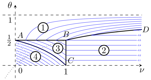
Figure 4: Summary of the convergence rates $\omega(\nu,\theta)$. The domain $(0,\infty)\times(0,1)$ is divided into four regimes by the solid black lines. Contours of $\omega$ are given in blue lines. In Regime 1, $\omega=-\nu(1-\theta)$. In Regime 2, $\omega=-\theta$. In Regimes 3 and 4, $\omega=1-2\theta-\nu+\nu\theta=-\nu(1-\theta)+(1-2\theta)=-\theta+(1-\theta)(1-\nu)$. The values of $\omega$ continuously extend to the boundaries between regimes. Arc BD is from the hyperbola $\theta=\nu/(\nu+1)$ which is extended by the dotted line. $\omega$ approaches its supremum along the ridge $B\to D$. Logarithm factor in (A.3) only appears on the line segments AB and BC including point B. In Regime 4 including Arc AC (which is $\theta=(1-\nu)/(2-\nu)$), $\omega\geq 0$ and the integral in (A.3) does not converge to zero as $b\to\infty$.

Proof of Lemma 14.

To verify the estimate (A.3), we divide the integral interval into $[1,b/2]$ and $[b/2,b]$, and denote $\Upsilon_{1}^{\mathsf{OL}}$ and $\Upsilon_{2}^{\mathsf{OL}}$ the associated parts of the integral in (A.3), respectively. First,

$$\Upsilon^{\mathsf{OL}}_{1}\leq \frac{1}{1+(b^{1-\theta}-(b/2)^{1-\theta})^{\nu}}\int^{b/2}_{1}u^{-2\theta}du$$

$$\leq \frac{b^{-\nu(1-\theta)}}{(1-2^{\theta-1})^{\nu}}\times\left\{\begin{array}[]{ll}\frac{(b/2)^{1-2\theta}}{1-2\theta},&\mbox{when }0<\theta<1/2,\\ \log\frac{b}{2},&\mbox{when }\theta=1/2,\\ \frac{1}{2\theta-1},&\mbox{when }1/2<\theta<1,\end{array}\right.$$ (A.11)

$$\leq \frac{1}{(1-2^{\theta-1})^{\nu}}\times\left\{\begin{array}[]{ll}\displaystyle\frac{2^{2\theta-1}}{1-2\theta}b^{1-2\theta-\nu+\nu\theta},&0<\theta<1/2,\\ \displaystyle b^{-\nu/2}\log b,&\theta=1/2,\\ \displaystyle\frac{1}{2\theta-1}b^{-\nu(1-\theta)},&1/2<\theta<1.\end{array}\right.$$ (A.15)

Second, to estimate $\Upsilon_{2}^{\mathsf{OL}}$, we change the variable as $\xi=b^{1-\theta}-u^{1-\theta}$ to give $d\xi=-(1-\theta)u^{-\theta}du$. Therefore,

$$\Upsilon_{2}^{\mathsf{OL}} =\int^{b}_{b/2}\frac{u^{-2\theta}du}{1+(b^{1-\theta}-u^{1-\theta})^{\nu}}=\int^{b^{1-\theta}-(b/2)^{1-\theta}}_{0}\frac{u^{-\theta}d\xi}{(1+\xi^{\nu})(1-\theta)}$$

$$\leq\frac{(b/2)^{-\theta}}{1-\theta}\int^{b^{1-\theta}}_{0}\frac{d\xi}{1+\xi^{\nu}}.$$

Recall that for any $\nu>0$ and $\tau\geq 1$,

$$\int^{\tau}_{0}\frac{d\xi}{1+\xi^{\nu}}\leq 1+\int^{\tau}_{1}\xi^{-\nu}d\xi\leq\left\{\begin{array}[]{ll}1+\frac{\tau^{1-\nu}-1}{1-\nu}\leq\frac{1}{1-\nu}\tau^{1-\nu},&0<\nu<1,\\ 1+\log\tau,&\nu=1,\\ 1+\frac{1-\tau^{1-\nu}}{\nu-1}\leq\frac{\nu}{\nu-1},&\nu>1.\\ \end{array}\right.$$ (A.19)

Therefore,

$$\Upsilon_{2}^{\mathsf{OL}}\leq\left\{\begin{array}[]{ll}\displaystyle\frac{2^{\theta}}{(1-\theta)(1-\nu)}b^{1-2\theta-\nu+\nu\theta},&0<\nu<1,\\ \frac{2^{\theta}}{1-\theta}\left(\frac{1}{\log 2}+1-\theta\right)b^{-\theta}\log b,&\nu=1,\\ \frac{2^{\theta}\nu}{(1-\theta)(\nu-1)}b^{-\theta},&\nu>1.\displaystyle\displaystyle\end{array}\right.$$ (A.23)

Now we merge (A.15) and (A.23) to derive (A.3). Note that the bounds of $\Upsilon_{1}^{\mathsf{OL}}$ are divided according to $\theta$, while the bounds of $\Upsilon_{2}^{\mathsf{OL}}$ are divided according to $\nu$, so the merging appears complicated. Figure 4 provides a clear picture.

• Case 1: $\nu/(\nu+1)\leq\theta<1$ and $\theta>1/2$. This corresponds to Regime 1 in Figure 4, including the boundary BD but excluding line segment AB and point B. Below we show that $\omega=-\nu(1-\theta)$. In fact, now $\Upsilon_{1}^{\mathsf{OL}}\leq(1-2^{\theta-1})^{-\nu}(2\theta-1)^{-1}b^{-\nu(1-\theta)}$. When $0<\nu<1$, $\theta>1/2$ implies $1-2\theta-\nu+\nu\theta<-\nu(1-\theta)$, so $\Upsilon_{2}^{\mathsf{OL}}\leq 2^{\theta}(1-\theta)^{-1}(1-\nu)^{-1}b^{-\nu(1-\theta)}$. When $\nu=1$, recall that

  $$\max_{1\leq u<\infty}u^{-a}\log u=\frac{1}{ea},\quad\mbox{for any }a>0,$$ (A.24)

  where the maximum is achieved at $u=e^{1/a}$. Since $\theta>1/2$, $b^{-\theta+(1-\theta)}\log b\leq\frac{1}{e(2\theta-1)}$, and we have

  $$\Upsilon_{2}^{\mathsf{OL}}\leq\frac{2^{\theta}}{1-\theta}\left(\frac{1}{\log 2}+1-\theta\right)\frac{b^{-(1-\theta)}}{e(2\theta-1)}.$$

  When $\nu>1$, the condition $\nu/(\nu+1)\leq\theta$ implies $-\theta\leq-\nu(1-\theta)$, so $\Upsilon_{2}^{\mathsf{OL}}\leq 2^{\theta}\nu(1-\theta)^{-1}(\nu-1)^{-1}b^{-\nu(1-\theta)}$. We have proved that

  $$\int^{b}_{1}\frac{u^{-2\theta}du}{1+(b^{1-\theta}-u^{1-\theta})^{\nu}}=\Upsilon_{1}^{\mathsf{OL}}+\Upsilon_{2}^{\mathsf{OL}}\leq C^{\mathsf{OL}}_{0}b^{-\nu(1-\theta)},$$

  with

  $$C_{0}^{\mathsf{OL}}=\frac{(1-2^{\theta-1})^{-\nu}}{(2\theta-1)}+\left\{\begin{array}[]{ll}\displaystyle\frac{2^{\theta}(\nu+1)}{(1-\theta)|1-\nu|},&\nu>0\mbox{ and }\nu\neq 1,\\ \displaystyle\frac{2^{\theta}}{(1-\theta)(e(2\theta-1))}\left(\frac{1}{\log 2}+1-\theta\right),&\nu=1.\displaystyle\end{array}\right.$$ (A.27)

• Case 2: $\nu>1$ and $0<\theta<\nu/(\nu+1)$. This corresponds to Regime 2 in Figure 4, excluding the boundaries BC and BD. Below we show that $\omega=-\theta$. In fact, in this regime $\Upsilon_{2}^{\mathsf{OL}}\leq 2^{\theta}\nu(1-\theta)^{-1}(\nu-1)^{-1}b^{-\theta}$. When $0<\theta<1/2$, $1-2\theta-\nu+\nu\theta=-\theta+(1-\theta)(1-\nu)<-\theta$, so $\Upsilon_{1}^{\mathsf{OL}}\leq\frac{2^{2\theta-1}}{(1-2^{\theta-1})^{\nu}(1-2\theta)}b^{-\theta}$. When $\theta=1/2$, we use (A.24) to see $b^{-\frac{\nu}{2}+\frac{1}{2}}\log b\leq\frac{2}{e(\nu-1)}$, so $\Upsilon_{1}^{\mathsf{OL}}\leq(1-2^{\theta-1})^{-\nu}\frac{2}{e(\nu-1)}b^{-\theta}$. When $1/2<\theta<1$, $\theta<\nu/(\nu+1)$ implies $-\nu(1-\theta)<-\theta$, so $\Upsilon_{1}^{\mathsf{OL}}\leq(1-2^{\theta-1})^{-\nu}(2\theta-1)^{-1}b^{-\theta}$. We have proved that

  $$\int^{b}_{1}\frac{u^{-2\theta}du}{1+(b^{1-\theta}-u^{1-\theta})^{\nu}}=\Upsilon_{1}^{\mathsf{OL}}+\Upsilon_{2}^{\mathsf{OL}}\leq C^{\mathsf{OL}}_{0}b^{-\theta},$$

  with

  $$C_{0}^{\mathsf{OL}}=\frac{2^{\theta}\nu}{(1-\theta)(\nu-1)}+\frac{1}{(1-2^{\theta-1})^{\nu}}\times\left\{\begin{array}[]{ll}2^{2\theta-1}/(1-2\theta),&0<\theta<1/2,\\ \frac{2}{e(\nu-1)},&\theta=1/2,\\ 1/(2\theta-1),&1/2<\theta<1.\end{array}\right.$$ (A.31)

• Case 3: $0<\theta<1/2$ and $0<\nu<1$. This corresponds to Regimes 3 and 4 in Figure 4, including Arc AC but excluding boundaries AB, BC, and point B. Now it is obvious that $\Upsilon_{1}^{\mathsf{OL}}+\Upsilon_{2}^{\mathsf{OL}}\leq C_{0}^{\mathsf{OL}}b^{1-2\theta-\nu+\nu\theta}$, with

  $$C_{0}^{\mathsf{OL}}=\frac{2^{2\theta-1}}{(1-2^{\theta-1})^{\nu}(1-2\theta)}+\frac{2^{\theta}}{(1-\theta)(1-\nu)}.$$ (A.32)

• Case 4: $\theta=1/2$ and $0<\nu\leq 1$. This corresponds to line segment AB, including point B. Now $-\nu(1-\theta)=-\nu/2$, $b^{-\nu/2}\log b\geq b^{-\theta}\log b\geq b^{-\theta}\log 2$, and $1-2\theta-\nu+\nu\theta=-\nu(1-\theta)$. So

  $$\Upsilon_{2}^{\mathsf{OL}}\leq b^{-\nu(1-\theta)}(\log b)\times\left\{\begin{array}[]{ll}\displaystyle\frac{2^{\theta}}{1-\theta}\left(\frac{1}{\log 2}+1-\theta\right),&\nu=1,\\ \displaystyle\frac{2^{\theta}\nu}{(1-\theta)(\nu-1)\log 2},&0<\nu<1,\end{array}\right.$$

  and $\Upsilon_{1}^{\mathsf{OL}}\leq(1-2^{\theta-1})^{-\nu}b^{-\nu/2}\log b$. So, $\Upsilon_{1}^{\mathsf{OL}}+\Upsilon_{2}^{\mathsf{OL}}\leq C_{0}^{\mathsf{OL}}b^{-\nu(1-\theta)}\log b$ with

  $$C_{0}^{\mathsf{OL}}\leq\frac{1}{(1-2^{\theta-1})^{\nu}}+\left\{\begin{array}[]{ll}\displaystyle\frac{2^{\theta}}{1-\theta}\left(\frac{1}{\log 2}+1-\theta\right),&\nu=1,\\ \displaystyle\frac{2^{\theta}\nu}{(1-\theta)(\nu-1)\log 2},&0<\nu<1.\end{array}\right.$$ (A.35)

• Case 5: $\nu=1$ and $0<\theta<1/2$. This corresponds to line segment BC, excluding point B. In this case, $1-2\theta-\nu+\nu\theta=-\theta$. So $\Upsilon_{1}^{\mathsf{OL}}+\Upsilon_{2}^{\mathsf{OL}}\leq C_{0}^{\mathsf{OL}}b^{-\theta}\log b$ with

  $$C_{0}^{\mathsf{OL}}=\frac{2^{\theta}}{1-\theta}\left(\frac{1}{\log 2}+1-\theta\right)+\frac{2^{2\theta-1}}{(1-2^{\theta-1})^{\nu}(1-2\theta)\log 2}.$$ (A.36)

∎

References

- [1] Frank Bauer, Sergei Pereverzev, and Lorenzo Rosasco. On regularization algorithms in learning theory. J. Complexity, 23(1):52–72, 2007.
- [2] Raphaël Berthier, Francis Bach, and Pierre Gaillard. Tight nonparametric convergence rates for stochastic gradient descent under the noiseless linear model. Advances in Neural Information Processing Systems, 33:2576–2586, 2020.
- [3] Gilles Blanchard and Nicole Krämer. Optimal learning rates for kernel conjugate gradient regression. Advances in neural information processing systems, 23, 2010.
- [4] T. Tony Cai and Peter Hall. Prediction in functional linear regression. Ann. Statist., 34(5):2159–2179, 2006.
- [5] T. Tony Cai and Ming Yuan. Minimax and adaptive prediction for functional linear regression. J. Amer. Statist. Assoc., 107(499):1201–1216, 2012.
- [6] Andrea Caponnetto and Ernesto De Vito. Optimal rates for the regularized least-squares algorithm. Found. Comput. Math., 7(3):331–368, 2007.
- [7] Xiaming Chen, Bohao Tang, Jun Fan, and Xin Guo. Online gradient descent algorithms for functional data learning. J. Complexity, 70(101635):1–14, 2022.
- [8] Felipe Cucker and Ding-Xuan Zhou. Learning theory: an approximation theory viewpoint, volume 24 of Cambridge Monographs on Applied and Computational Mathematics. Cambridge University Press, Cambridge, 2007. With a foreword by Stephen Smale.
- [9] Aymeric Dieuleveut and Francis Bach. Nonparametric stochastic approximation with large step-sizes. Ann. Statist., 44(4):1363–1399, 2016.
- [10] Jun Fan, Fusheng Lv, and Lei Shi. An RKHS approach to estimate individualized treatment rules based on functional predictors. Math. Found. Comput., 2(2):169–181, 2019.
- [11] Xin Guo, Junhong Lin, and Ding-Xuan Zhou. Rates of convergence of randomized Kaczmarz algorithms in Hilbert spaces. Appl. Comput. Harmon. Anal., 61:288–318, 2022.
- [12] Zheng-Chu Guo, Shao-Bo Lin, and Ding-Xuan Zhou. Learning theory of distributed spectral algorithms. Inverse Problems, 33(7):074009, 29, 2017.
- [13] Zheng-Chu Guo and Lei Shi. Fast and strong convergence of online learning algorithms. Adv. Comput. Math, 45(5):2745–2770, 2019.
- [14] Zheng-Chu Guo and Lei Shi. Optimal rates for coefficient-based regularized regression. Appl. Comput. Harmon. Anal., 47(3):662–701, 2019.
- [15] Peter Hall and Joel L. Horowitz. Methodology and convergence rates for functional linear regression. Ann. Statist., 35(1):70–91, 2007.
- [16] Xuqing He and Hongwei Sun. Error analysis of classification learning algorithms based on lums loss. Math. Found. Comput., published online first, 2022.
- [17] Shao-Bo Lin, Xin Guo, and Ding-Xuan Zhou. Distributed learning with regularized least squares. J. Mach. Learn. Res., 18(1):3202–3232, 2017.
- [18] Loucas Pillaud-Vivien, Alessandro Rudi, and Francis Bach. Statistical optimality of stochastic gradient descent on hard learning problems through multiple passes. Advances in Neural Information Processing Systems, 31, 2018.
- [19] James O. Ramsay and Bernard W. Silverman. Fitting differential equations to functional data: Principal differential analysis. Springer, 2005.
- [20] Ingo Steinwart and Andreas Christmann. Support vector machines. Information Science and Statistics. Springer, New York, 2008.
- [21] Shuhua Wang and Baohuai Sheng. Error analysis of kernel regularized pairwise learning with a strongly convex loss. Math. Found. Comput., published online first, 2022.
- [22] Yiming Ying and Massimiliano Pontil. Online gradient descent learning algorithms. Found. Comput. Math., 8(5):561–596, 2008.
- [23] Ming Yuan and T. Tony Cai. A reproducing kernel Hilbert space approach to functional linear regression. Ann. Statist., 38(6):3412–3444, 2010.
- [24] Ding-Xuan Zhou. Derivative reproducing properties for kernel methods in learning theory. J. Comput. Appl. Math., 220(1-2):456–463, 2008.