Certifying Parity Reasoning Efficiently
Using Pseudo-Boolean Proofs

Abstract

The dramatic improvements in combinatorial optimization algorithms over the last decades have had a major impact in artificial intelligence, operations research, and beyond, but the output of current state-of-the-art solvers is often hard to verify and is sometimes wrong. For Boolean satisfiability (SAT) solvers proof logging has been introduced as a way to certify correctness, but the methods used seem hard to generalize to stronger paradigms. What is more, even for enhanced SAT techniques such as parity (XOR) reasoning, cardinality detection, and symmetry handling, it has remained beyond reach to design practically efficient proofs in the standard DRAT format. In this work, we show how to instead use pseudo-Boolean inequalities with extension variables to concisely justify XOR reasoning. Our experimental evaluation of a SAT solver integration shows a dramatic decrease in proof logging and verification time compared to existing DRAT methods. Since our method is a strict generalization of DRAT, and readily lends itself to expressing also 0-1 programming and even constraint programming problems, we hope this work points the way towards a unified approach for efficient machine-verifiable proofs for a rich class of combinatorial optimization paradigms.

1 Introduction

Since around the turn of the millennium, combinatorial optimization has been successfully applied to solve an ever increasing range of problems in e.g., resource allocation, scheduling, logistics, and disaster management [PDG13], and more recent applications in biology, chemistry, and medicine include, e.g., protein analysis and design [AAB⁺14, MWB08] and planning for kidney transplants [MO12, BvdKM⁺21]. Yet other examples are government auctions generating billions of dollars in revenue [LMS17], as well as allocation of education and work opportunities [Man16, MMT17] and matching of adoptive families with children [DGG⁺19].

As more and more such problems are dealt with using combinatorial optimization solvers, an urgent question is whether we can trust that the solutions computed by such algorithms are correct and complete. The answer, unfortunately, is currently a clear “no”: State-of-the-art solvers sometimes return “solutions” that do not satisfy the constraints or erroneously claim optimality of solutions [CKSW13, AGJ⁺18, GSD19]. This can be fatal for applications such as, e.g., chip design, compiler optimization, and combinatorial auctions, where correctness is absolutely crucial, not to speak about when human lives depend on finding the best solutions.

Conventional software testing has made little progress in addressing this problem, and formal verification techniques cannot handle the level of complexity of modern solvers. Instead, the most successful approach to date has been that of proof logging in the Boolean satisfiability (SAT) community, where solvers are required to be certifying [MMNS11] in the sense that they output not only a result but also a simple, machine-verifiable proof that this result is correct.

This does not certify the correctness of the solver itself, but it does mean that if it ever produces an incorrect answer (even if due to hardware errors), then this can be detected. Furthermore, such proofs can in principle be stored and audited later by a third party using independently developed software. A number of different proof logging formats such as RUP [GN03], TraceCheck [Bie06], DRAT [HHW13a, HHW13b, WHH14], GRIT [CFMSSK17], and LRAT [CFHH⁺17] have been developed, with DRAT now established as the standard in the SAT competitions [SAT].

A quite natural, and highly desirable, goal would be to extend these proof logging techniques to stronger combinatorial optimization paradigms such as pseudo-Boolean (PB) optimization, MaxSAT solving, mixed integer linear programming (MIP), and constraint programming (CP), but such attempts have had limited success. Either the proofs require trusting in powerful and complicated rules (as in, e.g., [VS10]), defeating simplicity and verifiability, or they have to justify such rules by long explanations, leading to an exponential slow-down (see [GS19]). In fact, even for SAT solvers a long-standing problem is that more advanced techniques for detecting and reasoning with parity constraints (a.k.a. exclusive or, or XOR, constraints), cardinality constraints, and symmetries have remained out of reach for efficient proof logging. Although in theory it might seem like there should be no problems—the DRAT proof system is extremely powerful, and can in principle justify such reasoning and much more with at most a polynomial amount of work [SB06, HHW15, PR16]—in practice the overhead seems completely prohibitive. Thus, a key challenge on the road to efficient proof logging for more general combinatorial optimization solvers would seem to be to design a method that can capture the full range of techniques used in modern SAT solvers.

1.1 Our Contribution

In this work, we present a new, efficient proof logging method for parity reasoning that is—perhaps somewhat surprisingly—based on pseudo-Boolean reasoning with $0$-$1$ integer linear inequalities. Though such inequalities might seem ill-suited to representing XOR constraints, this can be done elegantly by introducing auxiliary so-called extension variables [DGP04]. Using this observation, we strengthen the VeriPB tool [Ver] recently introduced in [EGMN20], which can be viewed as a generalization to pseudo-Boolean proofs of RUP [GN03]. Borrowing inspiration from [HKB17, BT19], we develop stronger, but still efficient, rules that can handle also extension variables, making VeriPB, in effect, into a strict generalization of DRAT.

We have implemented our method for representing XOR constraints and performing Gaussian elimination on such constraints in a library with a simple, clean interface for SAT solvers. As a proof of concept, we have also integrated it in MiniSat [ES04], which still serves as the foundation of many state-of-the-art SAT solvers. Our library also provides DRAT proof logging for XORs as described in [PR16], but with some optimizations, to allow for a comparative evaluation. Our experiments show that the overhead for proof logging, the size of the produced proofs, and the time for verification all go down by orders of magnitude for our pseudo-Boolean method compared to DRAT. Furthermore, the fact that PB reasoning forms the basis for solvers like Sat4j [LP10] and RoundingSat [EN18] means that our library can also empower such pseudo-Boolean solvers to reason with parities.

Since cardinality constraints are just a special case of PB constraints, it is clear that our method should suffice to justify the cardinality reasoning used in SAT solvers. The method presented in this paper is not sufficient for efficient proof logging of general symmetry breaking, but at least we can perform as efficiently for symmetry breaking as any approach using DRAT, since our proof system subsumes DRAT. More excitingly, the original VeriPB tool has already been shown to be capable of efficiently justifying a number of constraint programming techniques [EGMN20, GMN20, GMM⁺20]. Our optimistic interpretation is that pseudo-Boolean reasoning with extension variables shows great potential as a unified method of proof logging for SAT solving, pseudo-Boolean optimization, MaxSAT solving, constraint programming, and maybe even mixed integer programming.

1.2 Subsequent Developments

The last couple of years have witnessed quite significant developments in proof logging. Since the conference version of this paper appeared, our pseudo-Boolean proof logging method has been extended further to deal with fully general symmetry breaking in SAT solving [BGMN22], and also to support pseudo-Boolean solving using SAT solvers [GMNO22]. Furthermore, there have been promising preliminary results on providing proof logging for MaxSAT solvers [VWB22] and constraint programming solvers [GMN22].

The DRAT proof logging method has recently been extended to FRAT [BCH21], which allows to integrate different forms of reasoning. Proof logging using binary decision diagrams (BDDs) [Bry22], generating proofs in all of the DRAT, LRAT, and FRAT formats, has also been developed for pseudo-Boolean reasoning [BBH22] and parity reasoning [SB22]. Further evaluation will be needed to decide whether such clausal proof logging methods can be truly competitive with pseudo-Boolean proof logging.

1.3 Organization of This Paper

After some brief background in Section 2, we introduce the key technical notions needed for our new proof logging rules in Section 3 and show how they can be used to justify parity reasoning in Section 4 with a worked out example in Section 5. We present an experimental evaluation in Section 6 and provide some concluding remarks in Section 7.

2 Preliminaries

Let us start by quickly reviewing the required material on pseudo-Boolean reasoning, referring the reader to, e.g., [BN21] for more context. A few pieces of standard notation are that we write $\mathbb{N}=\{0,1,2,\ldots\}$ to denote non-negative integers and $\mathbb{N}^{+}=\mathbb{N}\setminus\{0\}$ to denote positive integers. For $n\in\mathbb{N}^{+}$, we write $[n]=\{1,2,\ldots,n\}$ to denote the set consisting of the first $n$ positive integers.

A literal $\ell$ over a Boolean variable $x$ is $x$ itself or its negation $\overline{x}=1-x$, where variables take values $0$ (false) or $1$ (true). For notational convenience, we define $\overline{\overline{x}}=x$. A pseudo-Boolean (PB) constraint $C$ over literals $\ell_{1},\dots,\ell_{n}$ is a $0$-$1$ linear inequality

$$\sum_{i=1}^{n}a_{i}\ell_{i}\geq A\enspace,$$ (2.1)

which without loss of generality we always assume to be in normalized form; i.e., all literals $\ell_{i}$ are over distinct variables and the coefficients $a_{i}$ and the degree (of falsity) $A$ are non-negative integers. Conversion to normalized form can be performed efficiently by using equalities $\overline{x}=1-x$ to rewrite the left-hand side of any inequality as a positive linear combination of literals, and so in what follows we will consider any pseudo-Boolean constraint and its normalized form to be one and the same constraint. We will use equality

$$\sum_{i=1}^{n}a_{i}\ell_{i} =A$$ (2.2a)

as syntactic sugar for the pair of inequalities

$$\sum_{i=1}^{n}a_{i}\ell_{i} \geq A$$ (2.2b)

$$\sum_{i=1}^{n}-a_{i}\ell_{i} \geq-A$$ (2.2c)

(but rewritten in normalized form) and the negation $\neg C$ of (2.1) is (the normalized form of)

$$\sum_{i=1}^{n}-a_{i}\ell_{i}\geq-A+1\enspace.$$ (2.3)

A pseudo-Boolean formula is a conjunction $F=\bigwedge_{j=1}^{m}C_{j}$ of pseudo-Boolean constraints. Note that a clause $\ell_{1}\lor\cdots\lor\ell_{k}$ is equivalent to the constraint $\ell_{1}+\cdots+\ell_{k}\geq 1$, so formulas in conjunctive normal form (CNF) are special cases of pseudo-Boolean formulas.

A (partial) assignment is a (partial) function from variables to $\{0,1\}$ and a substitution is a (partial) function from variables to literals or $\{0,1\}$. For an assignment or substitution $\rho{}$ we will use the convention $\rho(x{})=x{}$ for $x$ not in the domain of $\rho$, denoted $x{}\not\in\textit{dom}(\rho{})$, and define $\rho(\overline{x})=1-\rho(x)$. We also write $x\mapsto b$ instead of $\rho(x)=b$, where $b$ denotes $0$, $1$, or a literal, when $\rho$ is clear from context or is immaterial. Applying $\rho$ to a pseudo-Boolean constraint $C$ as in (2.1), denoted ${C\!\!\upharpoonright_{\rho}}$, yields the constraint obtained by substituting values for all assigned variables, shifting constants to the right-hand side, and adjusting the degree appropriately, i.e.,

$${C\!\!\upharpoonright_{\rho}}\,=\,{\textstyle\sum}_{i}a_{i}\rho(\ell_{i})\geq A$$ (2.4)

with appropriate normalization, and for a formula $F$ we define ${F\!\!\upharpoonright_{\rho}}=\bigwedge_{j}{C_{j}\!\!\upharpoonright_{\rho}}$. The normalized constraint $C$ is satisfied by $\rho$ if $\sum_{\rho(\ell_{i})=1}a_{i}\geq A$ (or, equivalently, if the restricted constraint (2.4) has a non-positive degree and is thus trivial). A PB formula is satisfied by $\rho$ if all constraints in it are, in which case it is satisfiable. If there is no satisfying assignment, the formula is unsatisfiable. Two formulas are equisatisfiable if they are both satisfiable or both unsatisfiable.

The cutting planes proof system as defined in [CCT87] is a method for iteratively deriving new constraints $C$ implied by a pseudo-Boolean formula $F$. Cutting planes contains rules for literal axioms

$$\ignorespaces\ignorespaces\leavevmode\lower 25.39555pt\hbox{\vbox{\hbox{\hskip 15.82574pt\hbox{\hskip 4.0pt\hbox{\rule{0.0pt}{8.0pt}}\hskip 4.0pt}}\vskip 2.0pt\nointerlineskip\hbox{\hskip 0.0pt\lower-0.2pt\hbox{}\hbox to39.65149pt{\xleaders\hrule\hfill}\lower-0.2pt\hbox{}}\vskip 2.0pt\nointerlineskip\hbox{\hbox{\hskip 4.0pt\hbox{$\ \ell_{i}\geq 0\ $}\hskip 4.0pt}}}}\ignorespaces\ ,$$ (2.5)

and linear combinations

$$\ignorespaces\ignorespaces\ignorespaces\leavevmode\lower 32.72234pt\hbox{\vbox{\hbox{\hskip 1.03319pt\hbox{\hbox{\hskip 4.0pt\hbox{$\textstyle\sum_{i}a_{i}\ell_{i}\geq A$}\hskip 4.0pt}\hbox{\hskip 14.45377pt}\hbox{\hskip 4.0pt\hbox{$\textstyle\sum_{i}b_{i}\ell_{i}\geq B$}\hskip 4.0pt}}}\vskip 2.0pt\nointerlineskip\hbox{\hskip 0.0pt\lower-0.2pt\hbox{}\hbox to123.149pt{\xleaders\hrule\hfill}\lower-0.2pt\hbox{}}\vskip 2.0pt\nointerlineskip\hbox{\hbox{\hskip 4.0pt\hbox{$\textstyle\sum_{i}({c_{A}}{a}_{i}+{c_{B}}{b}_{i})\ell_{i}\geq{c_{A}}{A}+{c_{B}}{B}$}\hskip 4.0pt}}}}\ignorespaces\ \ \ [\,c_{A},c_{B}\in\mathbb{N}\,]\enspace.$$ (2.6)

For notational convenience, in this paper we will sometimes use linear combinations of equalities as in (2.2a), which is just a shorthand for taking pairwise linear combinations of inequalities of the form (2.2b) and (2.2c), respectively. There is also a rule for division

$$\ignorespaces\ignorespaces\leavevmode\lower 32.72234pt\hbox{\vbox{\hbox{\hskip 20.16086pt\hbox{\hskip 4.0pt\hbox{$\textstyle\sum_{i}a_{i}\ell_{i}\geq A$}\hskip 4.0pt}}\vskip 2.0pt\nointerlineskip\hbox{\hskip 0.0pt\lower-0.2pt\hbox{}\hbox to93.83986pt{\xleaders\hrule\hfill}\lower-0.2pt\hbox{}}\vskip 2.0pt\nointerlineskip\hbox{\hbox{\hskip 4.0pt\hbox{$\textstyle\sum_{i}\lceil a_{i}/c\rceil\ell_{i}\geq\lceil A/c\rceil$}\hskip 4.0pt}}}}\ignorespaces\ \ \ [\,c\in\mathbb{N}^{+}\,]$$ (2.7)

(where we note that the soundness of this rule depends on that the pseudo-Boolean constraint is written in normalized form). As a toy example, the derivation

  $$6x+2y+3z\geq 5 x+2y+w\geq 1 c_{A}=1 c_{B}=2) 8x+6y+3z+2w\geq 7 c=3 3x+2y+z+w\geq 3$$              Linear combination (,                            Division ()                (2.8)

illustrates how these rules can be combined to obtain new constraints.

The proof system that we use for the proof logging in VeriPB also supports additional rules such as the saturation rule

$$\ignorespaces\ignorespaces\leavevmode\lower 32.72234pt\hbox{\vbox{\hbox{\hskip 21.80554pt\hbox{\hskip 4.0pt\hbox{$\sum_{i}a_{i}\ell_{i}\geq A$}\hskip 4.0pt}}\vskip 2.0pt\nointerlineskip\hbox{\hskip 0.0pt\lower-0.2pt\hbox{}\hbox to95.46259pt{\xleaders\hrule\hfill}\lower-0.2pt\hbox{}}\vskip 2.0pt\nointerlineskip\hbox{\hbox{\hskip 4.0pt\hbox{$\sum_{i}\min(a_{i},A)\cdot\ell_{i}\geq A$}\hskip 4.0pt}}}}\ignorespaces\enspace,$$ (2.9)

which is not part of the cutting planes proof system defined in [CCT87] but was introduced in the context of pseudo-Boolean solving in [CK05]. For example, from the constraint $8x+6y+3z+2w\geq 7$ in the example above it is possible to derive $7x+6y+3z+2w\geq 7$ via saturation. While this might not be clear from a small example like this, the division and saturation rules are incomparable in strength [GNY19].

For pseudo-Boolean formulas $F$, $F^{\prime}$ and constraints $C$, $C^{\prime}$, we say that $F$ implies or models $C$, denoted $F\models C$, if any assignment satisfying $F$ must also satisfy $C$, and we write $F\models F^{\prime}$ if $F\models C^{\prime}$ for all $C^{\prime}\in F^{\prime}$. It is not hard to see that any collection of constraints $F^{\prime}$ derived (iteratively) from $F$ by cutting planes are implied in this sense, and so it holds that $F$ and $F\land F^{\prime}$ are equisatisfiable. A particularly simple type of implication is when a constraint $C^{\prime}$ can be derived from some other constraint $C$ using only addition of literal axioms as in (2.5). When this is is the case, we will say that $C^{\prime}$ is implied syntactically by $C$.

A constraint $C$ is said to unit propagate the literal $\ell$ under $\rho$ if ${C\!\!\upharpoonright_{\rho}}$ cannot be satisfied unless $\ell\mapsto 1$. During unit propagation on $F$ under $\rho$, we extend $\rho$ iteratively by any propagated literals $\ell\mapsto 1$ until an assignment $\rho^{\prime}$ is reached under which no constraint $C\in F$ is propagating, or under which some constraint $C$ propagates a literal that has already been assigned to the opposite value. The latter scenario is referred to as a conflict, since $\rho^{\prime}$ violates the constraint $C$ in this case, and $\rho^{\prime}$ is called a conflicting assignment.

Using the generalization of [GN03] in [EGMN20], we say that $F$ implies $C$ by reverse unit propagation (RUP), and write $\mathit{RUP}(F,C)$, if $F\land\neg C$ unit propagates to conflict under the empty assignment. It is not hard to see that $\mathit{RUP}(F,C)$ implies $F\models C$, but the opposite direction is not necessarily true. Cutting planes as defined above is not only sound in the sense that it can only derived implied constraints, but it is also implicationally complete, which means that if a pseudo-Boolean formula $F$ implies a constraint $C$, then there is also a cutting planes derivation of $C$ from $F$. This holds, in particular, if $C$ is RUP with respect to $F$. However, it might not always be obvious how to construct such a derivation, and therefore we can add a derivation rule for adding RUP constraints as a convenient shorthand. An important special case of completeness is that if a set of pseudo-Boolean constraints $F$ is unsatisfiable, then there exists a cutting planes derivation of the contradiction $0\geq 1$ from $F$, which we refer to as a proof of unsatisfiability, or refutation, of $F$.

3 Redundance-Based Strengthening

In order to provide proof logging for parity reasoning, we need the ability not only to perform cutting planes reasoning, but also to introduce fresh variables not occurring in the formula $F$ under consideration. In particular, we want to be able to use a fresh variable $y$ to encode the reification of a constraint $\sum_{i}a_{i}\ell_{i}\geq A$, i.e., that $y$ is true if and only if the constraint is satisfied. We will use the shorthand

$$y\Leftrightarrow{\textstyle\sum}_{i}a_{i}\ell_{i}\geq A$$ (3.1)

to denote the two constraints

$$A\overline{y}+{\textstyle\sum}_{i}a_{i}\ell_{i} \geq A$$ (3.2a)

$$\bigl{(}-A\!+\!1\!+\!{\textstyle\sum}_{i}a_{i}\bigr{)}\cdot y+{\textstyle\sum}_{i}a_{i}\overline{\ell}_{i} \geq-A+1+{\textstyle\sum}_{i}a_{i}$$ (3.2b)

enforcing this condition (which is the case under the the assumption that the constraint $\sum_{i}a_{i}\ell_{i}\geq A$ is written in normalized form). By way of a concrete example, the reification of the constraint

$$x_{1}+x_{2}+x_{3}\geq 2$$ (3.3)

using $y$ is encoded as

$$2\overline{y}+x_{1}+x_{2}+x_{3} \geq 2$$ (3.4a)

$$2y+\overline{x}_{1}+\overline{x}_{2}+\overline{x}_{3} \geq 2$$ (3.4b)

in pseudo-Boolean form. Note that introducing such constraints maintains equisatisfiability provided that the reification variable $y$ does not appear in any other constraint, since any assignment to the literals $\ell_{i}$ will satisfy either (3.2a) or (3.2b), which allows us to assign $y$ so that the other constraint is also satisfied.

More generally, it would be convenient to allow the “derivation” of any constraint $C$ from $F$ such that $F$ and $F\land C$ are equisatisfiable—in which case we say that $C$ is redundant with respect to $F$—regardless of whether $F\models C$ holds or not. A moment of thought reveals that such a completely generic rule would be too good to be true—for any unsatisfiable formula $F$ we would then be able to “derive” contradiction (say, $0\geq 1$) in just one step, and such derivations would be hard to check for correctness. What we need, therefore, is a sufficient criterion for redundancy of pseudo-Boolean constraints that is simple to verify. To this end, we generalize the characterization of redundancy in [HKB17, BT19] from CNF formulas to pseudo-Boolean formulas as follows.

Proposition 3.1 (Substitution redundancy).

A pseudo-Boolean constraint $C$ is redundant with respect to the formula $F$ if and only if there is a substitution $\omega$, called a witness, for which it holds that

$$F\land\neg C\models{(F\land C)\!\!\upharpoonright_{\omega}}\enspace.$$

Proof.

($\Rightarrow$) Suppose $C$ is redundant. If $F$ is unsatisfiable, then for any constraint $C^{\prime}$ it vacuously holds that $F\models C^{\prime}$. Hence, any substitution $\omega$ fulfils the condition. If $F$ is satisfiable, then $F\land C$ must also be satisfiable as $C$ is redundant by assumption. If we choose $\omega$ to be a satisfying assignment for $F\land C$, the implication in the proposition again vacuously holds since ${(F\land C{})\!\!\upharpoonright_{\omega}}$ is fixed to true.

($\Leftarrow$) Suppose now that $\omega$ is such that $F\land\neg C\models{(F\land C)\!\!\upharpoonright_{\omega}}$. If $F$ is unsatisfiable, then every constraint is redundant and there is nothing to check. Otherwise, let $\alpha$ be a (total) satisfying assignment for $F$. If $\alpha$ also satisfies $C$, then clearly the constraint is redundant. Now consider the case that $\alpha$ does not satisfy $C$. If so, $\alpha$ must satisfy $\neg C$ and hence, by the assumed implication, also ${(F\land C{})\!\!\upharpoonright_{\omega}}$. But then the assignment $\beta$ defined by

$$\beta(x)=\begin{cases}\alpha(x)&\text{if $x\not\in\textit{dom}(\omega)$,}\\ \alpha(\omega(x))&\text{otherwise,}\end{cases}$$ (3.5)

satisfies both $C$ and $F$ (since ${(F\land C{})\!\!\upharpoonright_{\beta}}={({(F\land C{})\!\!\upharpoonright_{\omega}})\!\!\upharpoonright_{\alpha}}$ by construction), so $F\land C$ is satisfiable. ∎

We remark that this proof does not make use of that we are operating with a pseudo-Boolean constraint $C$—we only need that the negation $\neg C$ is easy to represent in the same formalism. Thus, the argument generalizes to other types of constraints with this property (such as, for instance, polynomial equations over finite fields when evaluated on Boolean inputs $\{0,1\}^{n}$, as in the polynomial calculus proof system [CEI96, ABRW02] formalizing Gröbner basis computations).

Let us return to our example reification of the constraint in (3.3) and show how this can be derived using substitution redundancy. Let us write $C_{\ref{eq:reification-example-encoding-1}}$ for the constraint in (3.4a) and $C_{\ref{eq:reification-example-encoding-2}}$ for (3.4b), where $y$ is fresh with respect to the current formula $F$. To show that $C_{\ref{eq:reification-example-encoding-2}}$ is substitution redundant with respect to $F$ we choose the witness $\omega=\{y\mapsto 1\}$, which clearly satisfies $C_{\ref{eq:reification-example-encoding-2}}$. Since $y$ does not appear in $F$ we have ${F\!\!\upharpoonright_{\omega}}=F$, and so the implication $F\land\neg C_{\ref{eq:reification-example-encoding-2}}\models{(F\land C_{\ref{eq:reification-example-encoding-2}})\!\!\upharpoonright_{\omega}}$ vacuously holds. Showing that $C_{\ref{eq:reification-example-encoding-1}}$ is substitution redundant with respect to $F\land C_{\ref{eq:reification-example-encoding-2}}$ is a bit more interesting. For this we choose $\omega=\{y\mapsto 0\}$, which satisfies $C_{\ref{eq:reification-example-encoding-1}}$ and again leaves $F$ unchanged. Thus, the only implication for which we need to do some work is $F\land C_{\ref{eq:reification-example-encoding-2}}\land\neg C_{\ref{eq:reification-example-encoding-1}}\models{C_{\ref{eq:reification-example-encoding-2}}\!\!\upharpoonright_{\omega}}$. The negation of $C_{\ref{eq:reification-example-encoding-1}}$ is

$$-2\overline{y}-x_{1}-x_{2}-x_{3}\geq-1\enspace,$$ (3.6a)

or, converted to normalized form,

$$2y+\overline{x}_{1}+\overline{x}_{2}+\overline{x}_{3}\geq 4$$ (3.6b)

using the rewriting rule $\ell=1-\overline{\ell}$. Adding the literal axiom $\overline{y}\geq 0$ twice to $\neg C_{\ref{eq:reification-example-encoding-1}}$, and using rewriting again to cancel $y+\overline{y}=1$, we obtain

$$\overline{x}_{1}+\overline{x}_{2}+\overline{x}_{3}\geq 2\enspace,$$ (3.7)

which is ${C_{\ref{eq:reification-example-encoding-2}}\!\!\upharpoonright_{\omega}}$. Hence, ${C_{\ref{eq:reification-example-encoding-2}}\!\!\upharpoonright_{\omega}}$ can be derived from $\neg C_{\ref{eq:reification-example-encoding-1}}$ by just adding literal axioms—or, in the terminology introduced in the preliminaries, $\neg C_{\ref{eq:reification-example-encoding-1}}$ syntactically implies ${C_{\ref{eq:reification-example-encoding-2}}\!\!\upharpoonright_{\omega}}$—and so it certainly holds that $F\land C_{\ref{eq:reification-example-encoding-2}}\land\neg C_{\ref{eq:reification-example-encoding-1}}\models{C_{\ref{eq:reification-example-encoding-2}}\!\!\upharpoonright_{\omega}}$. This completes the proof that $C_{\ref{eq:reification-example-encoding-1}}$ is redundant with respect to ${F\land C_{\ref{eq:reification-example-encoding-2}}}$.

In our proof system for pseudo-Boolean proof logging, we will include a redundance-based strengthening rule that allows to derive constraints that satisfy the condition in Proposition 3.1. In order to do so, we need to discuss how the implication in this substitution redundancy condition is to be verified. Whenever this rule is used, the user needs to explicitly specify a witness $\omega$, but this is not enough. Arbitrary implication checks are as hard to verify as determining satisfiability of a formula, and hence some kind of efficiently verifiable certificate that the implication indeed holds is necessary to be able to validate the proof. One way of providing such a certificate is to exhibit a cutting planes derivation establishing the validity of the implication, as in the example just presented. A more convenient alternative from a proof logging point of view is to follow the lead of DRAT and allow adding constraints without proof if the implication can be verified automatically, e.g., using reverse unit propagation. We describe our pseudo-Boolean version of this automatic verification method in Algorithm 1. It is easy to see that the condition in Proposition 3.1 is satisfied if Algorithm 1 issues a positive verdict: If the algorithm accepts because of $\mathit{RUP}(F,C)$, then $F\models C$ and it is in order to add the constraint. Otherwise, the algorithm will reject unless for all constraints $D$ in ${(F\land C{})\!\!\upharpoonright_{\omega}}$, i.e., all constraints on the right hand side of the implication in Proposition 3.1, it holds that (a) $D\in F$, (b) $\neg C$ implies $D$ syntactically, or (c) $\mathit{RUP}(F\land\neg C,D)$ evaluates to true. In all three cases it follows that $F\land C{}\models D$, as desired.

We remark that this algorithm is very similar to what is used for checking RAT clauses in DRAT proof verification, except that our unit propagation is on PB constraints rather than clauses and that we need the additional syntactic check on line 4 in Algorithm 1. To see why this extra step is necessary, note that if we used only unit propagation, then we would fail to certify the correctness of our example above. Assuming for simplicity that $F=\emptyset$, if we try to verify $C_{\ref{eq:reification-example-encoding-2}}\land\neg C_{\ref{eq:reification-example-encoding-1}}\models{C_{\ref{eq:reification-example-encoding-2}}\!\!\upharpoonright_{\omega}}$ by reverse unit propagation we get the constraints

$$2y+\overline{x}_{1}+\overline{x}_{2}+\overline{x}_{3} \geq 2 [\,\text{$C_{\ref{eq:reification-example-encoding-2}}$ in\leavevmode\nobreak\ \eqref{eq:reification-example-encoding-2}}\,]$$ (3.8a)

$$2y+\overline{x}_{1}+\overline{x}_{2}+\overline{x}_{3} \geq 4 [\,\text{$\neg C_{\ref{eq:reification-example-encoding-1}}$ in\leavevmode\nobreak\ \eqref{eq:neg-C-normalized}}\,]$$ (3.8b)

$$x_{1}+x_{2}+x_{3} \geq 2 [\,\text{negation of desired RUP constraint $\neg({C_{\ref{eq:reification-example-encoding-2}}\!\!\upharpoonright_{\omega}})$}\,]$$ (3.8c)

and although visual inspection shows that this collection of constraints is inconsistent, since it requires a majority of the variables $\{x_{1},x_{2},x_{3}\}$ to be true and false at the same time, unit propagation is too myopic to see this contradiction and only yields $y\mapsto 1$. Thanks to the fact that we instead use the stronger checks in Algorithm 1, we can automatically detect that the implication $C_{\ref{eq:reification-example-encoding-2}}\land\neg C_{\ref{eq:reification-example-encoding-1}}\models{C_{\ref{eq:reification-example-encoding-2}}\!\!\upharpoonright_{\omega}}$ holds. This means that to introduce extension variables encoding reifications $y\Leftrightarrow C$, we do not need to do anything more than just specifying witness assignments to the new variable as in the example above for constraints (3.4a) and (3.4b). For completeness, we write out the details in the general case for the constraints (3.2a) and (3.2b) in the next proposition.

1:procedure RedundancyCheck($F,C,\omega$) $\triangleright$ $C,\omega$ are given in the proof log

2:     if $\mathit{RUP}(F,C)$ then return $\mathtt{ACCEPT}$     

3:     for $D\in{(F\land C{})\!\!\upharpoonright_{\omega}}$ do

4:         if not $\bigl{(}D\in F$ or $\neg C$ implies $D$ syntactically or $\mathit{RUP}(F\land\neg C,D)\bigr{)}$  then

5:              return $\mathtt{REJECT}$              

6:     return $\mathtt{ACCEPT}$

Algorithm 1 Automatically checking substitution redundancy of $C$ with respect to $F$

Proposition 3.2.

Let $F$ be a pseudo-Boolean formula and $C$ be a pseudo-Boolean constraint, and suppose $y$ is a fresh variable that does not appear in $F$ or $C$. Then the constraints (3.2a) and (3.2b) encoding $y\Leftrightarrow C$ can both be derived and added to $F$ by the redundance-based strengthening rule using Algorithm 1 to verify the substitution redundancy conditions.

Proof.

Let us write $C_{\ref{eq:reification-encoding-1}}$ for the constraint in (3.2a) and $C_{\ref{eq:reification-encoding-2}}$ for (3.2b). To show that $C_{\ref{eq:reification-encoding-2}}$ is substitution redundant with respect to $F$ we choose the witness $\omega=\{y\mapsto 1\}$, which clearly satisfies $C_{\ref{eq:reification-encoding-2}}$. Since the negation of a satisfied constraint is contradiction, this means, technically speaking, that ${C_{\ref{eq:reification-encoding-2}}\!\!\upharpoonright_{\omega}}$ is RUP with respect to $F$. Since $y$ does not appear in $F$ we have ${D\!\!\upharpoonright_{\omega}}=D$ for all $D\in F$, which means that all constraints pass the check on Line 4 in Algorithm 1.

As in our example above, showing that $C_{\ref{eq:reification-encoding-1}}$ is substitution redundant with respect to $F\land C_{\ref{eq:reification-encoding-2}}$ requires slightly more work. Here we choose the witness $\omega=\{y\mapsto 0\}$, which satisfies $C_{\ref{eq:reification-encoding-1}}$ and again leaves $F$ unchanged, which means that implication checks for constraints in $F$ are again vacuous. The only constraint left to check is ${C_{\ref{eq:reification-encoding-2}}\!\!\upharpoonright_{\omega}}$, which is implied syntactically by $\neg C_{\ref{eq:reification-encoding-1}}$, as we will see next. The negation of $C_{\ref{eq:reification-encoding-1}}$ is

$$A\overline{y}+{\textstyle\sum}_{i}a_{i}\ell_{i} \leq A-1$$ (3.9a)

or

$$-A\overline{y}+{\textstyle\sum}_{i}-a_{i}\ell_{i} \geq-A+1\enspace,$$ (3.9b)

which in normalized form becomes

$$Ay+{\textstyle\sum}_{i}a_{i}\overline{\ell}_{i} \geq 1+{\textstyle\sum}_{i}a_{i}$$ (3.9c)

(rewriting using the equality $\ell=1-\overline{\ell}$ to obtain a positive linear combination of literals on the left-hand side of the inequality). Adding $A$ times the literal axiom $\overline{y}\geq 0$ to $\neg C_{\ref{eq:reification-encoding-1}}$ and applying cancellation $y+\overline{y}=1$, we obtain

$${\textstyle\sum}_{i}a_{i}\overline{\ell}_{i}\geq-A+1+{\textstyle\sum}_{i}a_{i}\enspace,$$ (3.10)

which is ${C_{\ref{eq:reification-encoding-2}}\!\!\upharpoonright_{\omega}}$. Hence, $\neg C_{\ref{eq:reification-encoding-1}}$ syntactically implies ${C_{\ref{eq:reification-encoding-2}}\!\!\upharpoonright_{\omega}}$, and so the condition on Line 4 is satisfied.

This concludes the proof that the conditions required to derive the constraints $C_{\ref{eq:reification-encoding-2}}$ and $C_{\ref{eq:reification-encoding-1}}$ by redundance-based strengthening can be checked efficiently by Algorithm 1 regardless of what the pseudo-Boolean formula $F$ is. ∎

4 Proof Logging for XOR Constraints

We now proceed to explain how the cutting planes proof system in Section 2 extended with the redundance-based strengthening rule in Section 3 can be used to certify the correctness of parity reasoning.

An XOR or parity constraint, i.e., an equality modulo 2, over $k$ Boolean variables is written as

$$x_{1}\oplus x_{2}\oplus\dots\oplus x_{k}=b$$ (4.1)

for $b\in\{0,1\}$. Note that we can assume that there is no parity constraint with a negated variable $\overline{x{}}$, because we can always substitute $\overline{x{}}=x{}\oplus 1$. Systems of XOR constraints can be handled in a solver through Gaussian elimination [SNC09, HJ12, LJN12b] or conflict analysis [LJN12a]. In this paper we will focus on the integration of Gaussian elimination into conflict-driven clause learning (CDCL) [BS97, MS99, MMZ⁺01], and so we start by a quick review of how the CDCL main loop works and how parity reasoning is included. The reader can consult the pseudocode in Algorithm 2 to complement the description below.

Algorithm 2 Conflict-driven clause learning with parity reasoning

1:procedure solve($F$)

2:     $\mathit{trail}\leftarrow\emptyset$

3:      $G\leftarrow$ detectParities($F$)

4:     $\mathcal{D}\leftarrow F$

5:     while True do

6:         ($\ell,C_{\mathrm{reason}}$) $\leftarrow$ propagate($\mathcal{D}$, $\mathit{trail}$)

7:         if $\ell=\mathtt{NULL}$ then ($\ell,C_{\mathrm{reason}}$) $\leftarrow$ propagateXOR($G$, $\mathit{trail}$)         

8:         if $\ell=\mathtt{NULL}$ then ($\ell,C_{\mathrm{reason}}$) $\leftarrow$ (nextDecision(), $\mathtt{NULL}$)         

9:         if $\ell=\mathtt{NULL}$ then return $\mathtt{SATISFIABLE}$          

10:         $\mathit{trail}$.push($\ell,C_{\mathrm{reason}}$)

11:         if hasConflict($\mathit{trail}$) then

12:              $C_{\mathrm{learned}}\leftarrow$ analyse($\mathit{trail}$)

13:              if $C_{\mathrm{learned}}=\bot$ then

14:                  return $\mathtt{UNSATISFIABLE}$

15:              else

16:                  $\mathcal{D}\leftarrow\mathcal{D}\cup\{C_{\mathrm{learned}}\}$

17:                  $\mathit{trail}\leftarrow$ backjump($\mathit{trail}$)                             

Let us first describe CDCL without parity reasoning, i.e., without the boldface italicized code on lines 3 and 7. When run on a formula $F$, the CDCL solver has a database $\mathcal{D}$ of clauses, which is initialized to the clauses in $F$. The solver also maintains a trail consisting of an ordered list of literals assigned to true together with reasons for these assignments. In what follows, it will be convenient to identify the trail with the assignment setting the literals on the trail to true. The trail is initialized to be empty.

The solver adds assigned literals to the trail, one by one, according to the following procedure. If some clause $C_{\mathrm{reason}}\in\mathcal{D}$ unit propagates an unassigned literal $\ell$ in the sense explained in Section 2 (which for a clause $C_{\mathrm{reason}}$ means that all literals in the clause except $\ell$ are falsified by the current trail), then the trail is extended by adding $\ell$ with $C_{\mathrm{reason}}$ as the reason clause explaining the propagation. (If several clauses propagate at the same time, then ties will be split in a somewhat arbitrary fashion depending on low-level details in the algorithm implementation.) Otherwise, the solver uses a decision heuristic to pick some literal to assign to true. Such a decision literal has no reason clause. If there is no literal left to assign, then this means that all variables have been assigned without violating any clause in $F$. In other words, a satisfying assignment has been found, and so the solver returns that the formula is satisfiable. Assuming instead that some literal has been added to the trail, this literal can lead to some clause $D\in\mathcal{D}$ being falsified by the trail. This is referred to as a conflict with $D$ as the conflict clause. When a conflict arises, a conflict analysis algorithm is called to derive a new clause $C_{\mathrm{learned}}$ from the conflict clause and the reason clauses currently on the trail. If the result of this conflict analysis is the empty clause $\bot$ without any literals, then contradiction has been derived and the solver returns that the formula is unsatisfiable. Otherwise, the clause $C_{\mathrm{learned}}$ is learned, i.e., added to the clause database, after which the solver backjumps by removing some literals from the trail until $C_{\mathrm{learned}}$ is no longer falsified. The details of exactly how backjumps are done are not relevant for our proof logging discussion, and there are also other details of CDCL that we are ignoring in this description, such as that the solver sometimes does restarts (which means resetting the trail to be empty) and sometimes performs database reduction (removing learned clauses from $\mathcal{D}$).

To add parity reasoning to CDCL, the solver is modified by first detecting implicit parity constraints in the CNF formula on line 3 in Algorithm 2. This can be done by checking syntactically if all clauses in the canonical clausal encoding of a parity constraint are present. For instance, the clauses

$$\{x_{1}\lor x_{2}\lor x_{3},\ \overline{x}_{1}\lor\overline{x}_{2}\lor x_{3},\ \overline{x}_{1}\lor x_{2}\lor\overline{x}_{3},\ x_{1}\lor\overline{x}_{2}\lor\overline{x}_{3}\}$$ (4.2a)

encode the parity constraint

$$x_{1}\oplus x_{2}\oplus x_{3}=1\enspace.$$ (4.2b)

Parity constraints detected in this way can then be used for Gaussian elimination, which generates new parity constraints. If all variables in a parity constraint except one is assigned by the trail, then the final variable is propagated to a value on line 7. It can also happen that a parity constraint is violated by the current trail, and detection of this condition is included on line 11. In both of these cases, the solver will need a reason or conflict clause, respectively, to justify the steps taken. Such a clause can be computed from the parity constraint in a straightforward way. Suppose, for example that from parity constraints $x_{1}\oplus x_{2}\oplus x_{3}=1$ and $x_{2}\oplus x_{3}\oplus x_{4}=1$ Gaussian elimination has derived $x_{1}\oplus x_{4}=0$, and suppose also that $x_{1}$ is assigned to true on the trail. Then $x_{4}$ will also propagate to true, and the reason clause provided for this will be $\overline{x}_{1}\lor x_{2}$.

There are many variations on how this general idea can be implemented. For instance, parity detection can also be run later during the search over the clause database $\mathcal{D}$, as done in CryptoMiniSat [Cry]. Another interesting question studied in [YM21] is whether it is better to propagate all clauses first (as in our pseudocode here) or all parity constraints first, or if the propagation on different types of constraints should be interleaved. However, such aspects are not relevant to how proof logging for parity reasoning should be designed, and our description in Algorithm 2 has been chosen mainly to make the exposition simple.

To provide proof logging for CDCL solvers with Gaussian elimination, we will need the four ingredients listed below:

1. XOR encoding: An efficient encoding of parity constraints as linear pseudo-Boolean constraints.

2. XOR reasoning: A method of deriving (the pseudo-Boolean encoding of) a new parity constraint from existing parity constraints.

3. Reason and conflict clause generation: The ability to prove the validity of reason and conflict clauses from the pseudo-Boolean encoding of parity constraints when such parity constraints give rise to propagations or conflicts, respectively.

4. Translation from CNF: A way of translating clausal encodings of parity constraints to pseudo-Boolean form (which is where we will need to go beyond cutting planes by using extension variables and redundance-based strengthening).

We will describe these components in detail in the rest of this section. In Section 5, we will then provide a worked-out example to illustrate how everything comes together to yield a method for CDCL solving with parity constraints.

4.1 Linear Pseudo-Boolean Encoding of Parity Constraints

Our encoding of parity constraints in linear pseudo-Boolean form is based on the observation in [DGP04] that for any partial assignment to the variables $x_{1},\ldots,x_{k}$, the parity constraint $x_{1}\oplus x_{2}\oplus\dots\oplus x_{k}=b$ as in (4.1) is satisfiable if and only if the $0-1$ integer linear equality

$$\sum_{i\in[k]}x_{i}=b+\sum_{i\in[\lfloor k/2\rfloor]}2y_{i}$$ (4.3)

is satisfiable, where $y_{1},\ldots,y_{\lfloor k/2\rfloor}$ are fresh variables not appearing in other constraints. Since the variables $y_{i}$ are otherwise unconstrained, the right-hand side can take any even (odd) value for $b=0$ ($b=1$) in the range from $0$ to $k$, and these are exactly the values that we want to allow for $\sum_{i\in[k]}x_{i}$. Recalling that any equality on the form (2.2a) can be represented with the two inequalities (2.2b) and (2.2c), we have obtained a representation of parity constraints as linear pseudo-Boolean inequalities.

In fact, we can generalize this by observing that if we let $\mathcal{B}$ denote any integer linear combination of variables, possibly also with a constant term, then the two inequalities

$$\sum_{i\in[k]}x_{i} \geq b+2\mathcal{B}$$ (4.4a)

$$\sum_{i\in[k]}-x_{i} \geq-b-2\mathcal{B}$$ (4.4b)

forming the equality $$\sum_{i\in[k]}x_{i}=b+2\mathcal{B}$$ imply the parity constraint

$$x_{1}\oplus x_{2}\oplus\cdots\oplus x_{k}=b\enspace.$$ (4.4c)

We will make repeated use of this observation below.

4.2 XOR Reasoning Using Pseudo-Boolean Constraints

Whenever we want to combine two XOR constraints to derive a new XOR constraint as is done during Gaussian elimination, we only need to add the pseudo-Boolean equalities corresponding to these two XOR constraints. Consider again our example derivation

  $$x_{1}\oplus x_{2}\oplus x_{3}=1 x_{2}\oplus x_{3}\oplus x_{4}=1 x_{1}\oplus x_{4}=0$$                               (4.5)

from before, and assume that the two premises are represented in pseudo-Boolean form as

$$x_{1}+x_{2}+x_{3} =2y_{1}+1$$ (4.6a)

and

$$x_{2}+x_{3}+x_{4} =2y_{2}+1$$ (4.6b)

for fresh variables $$y_{1} y_{2}$$ and . Then adding both equalities together we obtain

$$x_{1}+2x_{2}+2x_{3}+x_{4} =2y_{1}+2y_{2}+2$$ (4.6c)

which implies the desired XOR constraint by the observation we just made regarding (4.4a)–(4.4c). (Recall that a linear combination of equalities as in (2.2a) is a notational shorthand for taking pairwise linear combinations of inequalities (2.2b) and (2.2c).)

4.3 Reason and Conflict Clause Generation from XOR Constraints

As explained above, CDCL solvers justify all propagation and conflict analysis steps using clauses. If we want to use XOR constraints to propagate forced variable assignments or derive contradiction, then we need to provide clauses that justify such derivation steps, together with proof logging steps explaining why these clauses are valid. We next show how to derive such clauses from pseudo-Boolean encodings of XOR constraints.

Suppose we have a parity constraint encoded by inequalities of the form (4.4a)–(4.4b), and let ${\rho}$ be an assignment to the variables $x_{1},\ldots,x_{k}$ that is inconsistent with these inequalities because it falsifies the implied XOR constraint (4.4c). We want to derive from (4.4a)–(4.4b) a clause that is falsified under ${\rho}$. Let

$$\mathcal{F}(\rho)=\{i\in[k]\mid\rho(x_{i})=0\}$$ (4.7)

be the set of indices of variables assigned to false by ${\rho}$ and

$$\mathcal{T}(\rho)=\{j\in[k]\mid\rho(x_{j})=1\}$$ (4.8)

the indices of variables assigned to true . Using the literal axiom rule (2.5) we can derive (the normalized form of) the trivially true constraint

$$\sum_{i\in{\mathcal{F}(\rho)}}x_{i}+\sum_{j\in{\mathcal{T}(\rho)}}-x_{j}\geq-\lvert\mathcal{T}(\rho)\rvert\enspace,$$ (4.9)

which when added to (4.4a) yields

$$\sum_{i\in{\mathcal{F}(\rho)}}2x_{i}\geq b-\lvert\mathcal{T}(\rho)\rvert+2{\mathcal{B}}\enspace.{}$$ (4.10)

By assumption, we have that $b-\lvert\mathcal{T}(\rho)\rvert$ is odd, since otherwise $\rho$ would not falsify the XOR constraint implied by (4.4a)–(4.4b). All other terms in the inequality (4.10) are divisible by $2$. Hence, even though (4.10) is not presented in normalized form, we can see that if we apply the division rule (2.7) with divisor $2$, this will round up and increase the degree of falsity. This means that if we divide the constraint (4.10) and then multiply by $2$ (which is just a special case of the linear combination rule (2.6)), we get

$$\sum_{i\in{\mathcal{F}(\rho)}}2x_{i}\geq b-\lvert\mathcal{T}(\rho)\rvert+1+2{\mathcal{B}}\enspace.{}$$ (4.11)

We continue by adding (4.4b) to get

$$\sum_{i\in{\mathcal{F}(\rho)}}x_{i}-\sum_{j\in{\mathcal{T}(\rho)}}x_{j}\geq 1-\lvert\mathcal{T}(\rho)\rvert\enspace,$$ (4.12)

which is the same constraint as

$$\sum_{i\in{\mathcal{F}(\rho)}}x_{i}+\sum_{j\in{\mathcal{T}(\rho)}}\overline{x}_{j}\geq 1$$ (4.13)

after normalization. This last constraint, which is a disjunctive clause, is falsified under $\rho$ as desired, and so can serve as the conflict clause justifying why the assignment ${\rho}$ is inconsistent. Derivations of reason clauses for propagation work in a similar way—essentially, we can pretend that the propagated variable is set to the wrong value and then perform the derivation above to obtain a clause (4.13) that propagates the variable to the right value instead. An example for deriving a reason clause can be found towards the end of Section 5.

4.4 Translating Parity Constraints from CNF to Pseudo-Boolean Form

An XOR constraint as in (4.1) can be encoded into CNF in a canonical way by including for each of the $2^{{k}-1}$ assignments falsifying the constraint the disjunctive clause ruling out that assignment. For example, for $k=3$ and $b=1$ the parity constrain (4.2b) can be encoded by the clauses in (4.2a), which are written as the $0$-$1$ integer linear inequalities

$${x}_{1}+{x}_{2}+{x}_{3} \geq 1$$ (4.14a)

$$\overline{{x}}_{1}+\overline{{x}}_{2}+{x}_{3} \geq 1$$ (4.14b)

$$\overline{{x}}_{1}+{x}_{2}+\overline{{x}}_{3} \geq 1$$ (4.14c)

$${x}_{1}+\overline{{x}}_{2}+\overline{{x}}_{3} \geq 1$$ (4.14d)

in pseudo-Boolean form. Since the number of clauses in this canonical CNF encoding of an XOR constraint scales exponentially with the number of variables, it is only feasible to encode short XORs into CNF in this manner. However, it is possible to split up a long XOR constraint into multiple constant-size XORs using auxiliary variables $z_{i}$, which represent the partial parities up to and including ${x}_{i}$, i.e., $z_{i}=\sum_{{j}\in[i]}{x}_{j}\ (\bmod\ 2)$. In this way, a collection of parity constraints

$${x}_{1}\oplus{x}_{2}\oplus{z}_{2} =0$$ (4.15a)

$${z}_{2}\oplus{x}_{3}\oplus{z}_{3} =0$$ (4.15b)

$$\hskip 6.00006pt\vdots$$

$${z}_{k-2}\oplus{x}_{{k}-1}\oplus{x}_{k} =b$$ (4.15c)

can be used to represent the constraint (4.1). Assuming that we can split up parity constraints in this manner, we will only need to translate short parity constraints from CNF to pseudo-Boolean form. The original, long, parity constraints can then be recovered by XOR reasoning, just summing up the constraints (4.15a)–(4.15c), and proof logging for this derivation can be done as described in Section 4.2 above.

We perform the translation to the pseudo-Boolean XOR encoding from CNF in two steps, which we will describe in more detail after providing the general idea. The first step is to derive the constraint

$$\sum_{{i}\in[{k}]}{x}_{i}=\sum_{{i}\in[\lfloor{k}/2\rfloor]}2{y}_{i}+y^{\prime}\enspace,$$ (4.16)

where $y^{\prime}$ and $y_{i}$, $i\in[\lfloor{k}/2\rfloor]$, are all fresh variables. Note that adding the equality constraint (4.16) to any formula does not affect satisfiability, because we can always assign the fresh variables so that this additional constraint holds true. However, although the constraint (4.16) is redundant in the sense of Proposition 3.1, we cannot use the redundance-based strengthening rule to derive the constraint, because we do not have an efficient procedure for constructing a witness $\omega$ that is efficiently verifiable by Algorithm 1. Instead, we will introduce the auxiliary variables $y^{\prime}$ and $y_{i}$, $i\in[\lfloor{k}/2\rfloor]$, one by one, in a similar fashion to what was done in Section 3. We remark that an alternative to (4.16) would be to encode the sum $2\cdot\bigl{\lfloor}\frac{1}{2}\sum_{i\in[k]}x_{i}\bigr{\rfloor}$ of the $x_{i}$-variables rounded down to the nearest even integer as a sum of powers of $2$, resulting in an equality constraint

$$\sum_{i\in[k]}x_{i}=\sum_{i\in[\lceil\log_{2}(k/2)\rceil]}2^{i}{y}_{i}+y^{\prime}\enspace.$$ (4.17)

For parity constraints over a large number of variables, this encoding has a substantially smaller number of auxiliary variables. However, since we are recovering parity constraints from CNF, we only expect to have parity constraints over few variables, as the number of clauses in the CNF encoding is exponential in the number of variables.

The second step, once we have derived the equality constraint (4.16), is to brute-force over all possible assignments to the $x_{i}$-variables to derive the equality

$$y^{\prime}=b\enspace.$$ (4.18)

Summing the equalities (4.16) and (4.18), we obtain a constraint of the desired form (4.3). Note that since we are considering all possible assignments to the $x_{i}$-variables, this derivation will require an exponential number of derivation steps measured in the number of variables, but this is still polynomial measured in the number of clauses in the canonical CNF encoding of parity constraints. We now proceed to describe this process in detail.

(a) A 1-bit full adder.

(b) Chain of 1-bit full adders.

Figure 1: Using adders to encode parities of subsets of variables.

Step 1a:

To derive (4.16) we will construct a chain of $1$-bit full adders, as illustrated in Figure 1(b) for an adder with output carry bit $y$ and sum bit $z$. Let us start by showing how the encoding of a single adder can be derived. A $1$-bit full adder (shown in Figure 1(a)) computes the sum of three variables $x_{1},x_{2},x_{3}$ and returns the result as a binary number. This can be encoded using the pseudo-Boolean equality

$$2y+z=x_{1}+x_{2}+x_{3}\enspace.$$ (4.19)

Recalling the shorthand (3.1) for the two reification constraints (3.2a) and (3.2b), in order to obtain (4.19) we start by deriving

$$y \Leftrightarrow x_{1}+x_{2}+x_{3}\geq 2$$ (4.20a)

$$z \Leftrightarrow x_{1}+x_{2}+x_{3}-2y\geq 1$$ (4.20b)

for fresh variables $y$ and $z$ using redundance-based strengthening as described in Proposition 3.2. This means that we have now derived the four constraints

$$2\overline{{y}}+{x}_{1}+{x}_{2}+{x}_{3} \geq 2$$ (4.21a)

$$2y+\overline{{x}}_{1}+\overline{{x}}_{2}+\overline{{x}}_{3} \geq 2$$ (4.21b)

$$3\overline{{z}}+{x}_{1}+{x}_{2}+{x}_{3}+2\overline{{y}} \geq 3$$ (4.21c)

$$3{z}+\overline{{x}}_{1}+\overline{{x}}_{2}+\overline{{x}}_{3}+2{y} \geq 3$$ (4.21d)

when written as pseudo-Boolean inequalities in normalized form. To derive the less-than-or-equal part $2y+z\leq x_{1}+x_{2}+x_{3}$ of (4.19), which in normalized form is

$${x}_{1}+{x}_{2}+{x}_{3}+2\overline{{y}}+\overline{{z}}\geq 3\enspace,$$ (4.22a)

we take a linear combination of (4.21c) and $$2 3 2y+z\geq x_{1}+x_{2}+x_{3}$$ times (4.21a), followed by division by . In a similar fashion, to derive the greater-than-or-equal part of (4.19), or

$$\overline{{x}}_{1}+\overline{{x}}_{2}+\overline{{x}}_{3}+2{y}+{z}\geq 3$$ (4.22b)

in normalized form, we add together (4.21d) and $2$ times (4.21b) followed by division by $3$.

Step 1b:

To derive the equality constraint (4.16), we use a chain of $1$-bit full adders connected as in Figure 1(b), where we set $k^{\prime}=\lfloor k/2\rfloor$. The $x_{i}$-variables are used as inputs to the adders, and the final variable $x_{2k^{\prime}+1}$, which appears in the topmost adder, will only be there if the number of variables $k$ is odd. Otherwise, we replace $x_{2k^{\prime}+1}$ by $0$, so that the topmost adder only has $x_{2k^{\prime}}$ and $x_{2k^{\prime}-1}$ as input. (Formally, if $x_{2k^{\prime}+1}$ does not exist, then it is a fresh variable, and so we can derive the equality $x_{2k^{\prime}+1}=0$ by redundance-based strengthening before continuing as described below.) The output carry variables $y_{i}$, $i\in[k^{\prime}]$, and the final sum bit $y^{\prime}$ will be used to derive the equality (4.16), while the $z_{i}$-variables are intermediate parity bits. We apply the procedure in Step 1a to all adders to derive PB constraints on the form (4.22a) and (4.22b). After this, for the topmost adder in Figure 1(b) we have obtained

$$2y_{k^{\prime}}+z_{k^{\prime}}=x_{2{k^{\prime}}+1}+x_{2{k^{\prime}}}+x_{2{k^{\prime}}-1}\enspace,$$ (4.23a)

for the intermediate adders the equations

$$2y_{i}+z_{i}=z_{i+1}+x_{2i}+x_{2i-1}$$ (4.23b)

hold for $$i\in\{2,\dots,{k^{\prime}}-1\}$$, and for the bottom adder we get

$$2y_{1}+y^{\prime}=z_{2}+x_{2}+x_{1}\enspace.{}$$ (4.23c)

By adding the encoding of all $1$-bit adders, i.e., the equalities (4.23a)–(4.23c), we obtain

$$\sum_{i=1}^{k^{\prime}}2y_{i}+y^{\prime}+\sum_{i=2}^{k^{\prime}}z_{i}=\sum_{i=2}^{k^{\prime}}z_{i}+\sum_{i=1}^{2{k^{\prime}}+1}x_{i}\enspace,$$ (4.24)

where the sums $\sum_{i=2}^{k^{\prime}}z_{i}$ on each side cancel to produce the equality constraint (4.16) as desired.

Step 2:

The final step is to fix the value of ${y^{\prime}}$ in order to go from (4.16) to our final goal (4.3). That is, writing $y^{\prime}(b)=y^{\prime}$ if $b=1$ and $y^{\prime}(b)=\overline{y}^{\prime}$ if $b=0$, we wish to derive the PB constraint

$$y^{\prime}(b)\geq 1$$ (4.25)

forcing $y^{\prime}=b$. We will do so by considering all possible truth value assignments $\rho$ to the variables $x_{i}$, $i\in[k]$. In order to present the formal derivation, we first need to set up some notation.

For any assignment $\rho$ to a subset of the variables $x_{i}$, $i\in[k]$, let $\mathcal{F}(\rho)$ and $\mathcal{T}(\rho)$ be the indices of variables set to false and true by $\rho$, respectively, as defined in (4.7) and (4.8). Let us write $C_{\lnot{\rho}}$ to denote the unique clausal constraint

$$\sum_{i\in\mathcal{F}(\rho)}x_{i}+\sum_{j\in\mathcal{T}(\rho)}\overline{x}_{j}\geq 1$$ (4.26)

over all variables assigned by $\rho$ that is falsified by this assignment. We also extend this notation in the natural way to let $C_{\lnot{(\rho\,\cup\,\{y^{\prime}(b)\mapsto 0\})}}$ denote the clausal constraint

$$y^{\prime}(b)+\sum_{i\in\mathcal{F}(\rho)}x_{i}+\sum_{j\in\mathcal{T}(\rho)}\overline{x}_{j}\geq 1$$ (4.27)

that is falsified by $\rho$ if in addition $y^{\prime}(b)$ is set to false, i.e., $y^{\prime}$ is given the value $1-b$.

For any assignment $\rho$ such that $\sum_{i\in[k]}x_{i}\neq b\ (\bmod\ 2)$, we postulated above that the clause $C_{\lnot{\rho}}$ is in the formula, but for our argument here we only need the slightly weaker assumption that this clause can be obtained by reverse unit propagation on the constraints derived so far. Assuming that this holds, we can certainly derive $C_{\lnot{(\rho\,\cup\,\{y^{\prime}(b)\mapsto 0\})}}$ by RUP for all such assignments $\rho$. If instead $\rho$ is such that $\sum_{i\in[k]}x_{i}=b\ (\bmod\ 2)$, then extending $\rho$ by setting $y^{\prime}(b)=0$ means that (4.16) can no longer be satisfied, since $\rho$ assigns different parities to the left-hand and right-hand sides of this equality, and no assignment to the $y_{i}$-variables in $\sum_{{i}\in[\lfloor{k}/2\rfloor]}2y_{i}$ can change this. For such $\rho$ we can therefore proceed as in Section 4.3 to derive the clause $C_{\lnot{(\rho\,\cup\,\{y^{\prime}(b)\mapsto 0\})}}$ explaining why the assignment $\rho\,\cup\,\{y^{\prime}(b)\mapsto 0\}$ is inconsistent.

So far, we have shown how to derive clauses $C_{\lnot{(\rho\,\cup\,\{y^{\prime}(b)\mapsto 0\})}}$ in (4.27) for any assignment $\rho$ to all the $x_{i}$-variables. But once we have these clauses, the rest is routine. Let $\rho_{k-1}$ be any partial assignment to the $k-1$ first variables $x_{i}$, $i\in[k-1]$. Taking the previously derived constraints $C_{\lnot{(\rho_{k-1}\cup\{x_{k}\mapsto 0,\,y^{\prime}(b)\mapsto 0\})}}$ and $C_{\lnot{(\rho_{k-1}\cup\{x_{k}\mapsto 1,\,y^{\prime}(b)\mapsto 0\})}}$, which is what we write by mild abuse of notation to denote the clausal constraints

$$y^{\prime}(b)+x_{k}+\sum_{i\in\mathcal{F}(\rho_{k-1})}x_{i}+\sum_{j\in\mathcal{T}(\rho_{k-1})}\overline{x}_{j} \geq 1$$ (4.28a)

and

$$y^{\prime}(b)+\overline{x}_{k}+\sum_{i\in\mathcal{F}(\rho_{k-1})}x_{i}+\sum_{j\in\mathcal{T}(\rho_{k-1})}\overline{x}_{j} \geq 1\enspace,$$ (4.28b)

respectively (which agree on all literals except that the variable $x_{k}$ appears with opposite signs), adding these constraints, and then dividing by $2$ yields

$$y^{\prime}(b)+\sum_{i\in\mathcal{F}(\rho_{k-1})}x_{i}+\sum_{j\in\mathcal{T}(\rho_{k-1})}\overline{x}_{j}\geq 1\enspace,$$ (4.29)

i.e., the clause $C_{\lnot{(\rho_{k-1}\,\cup\,\{y^{\prime}(b)\mapsto 0\})}}$. We can eliminate the variable $x_{k}$ in this way by deriving clauses (4.29) for all assignments $\rho_{k-1}$ to $x_{i}$, $i\in[k-1]$. (A technical side note is that the constraint (4.29) follows by reverse unit propagation on (4.28a) and (4.28b), and so we could avoid a syntactic derivation by just claiming it as a RUP constraint. However, when there is a simple explicit derivation like above it is often preferable to use such a derivation instead, since this tends to make proof verification faster, and as we will see in Section 5 there is an elegant way of chaining all derivations of this type together on a single proof line.)

Next, we consider all assignments $\rho_{k-2}$ to $x_{i}$, $i\in[k-2]$, and repeat the derivation of clauses (4.29) from (4.28a) and (4.28b) to obtain clauses $C_{\lnot{(\rho_{k-2}\,\cup\,\{y^{\prime}(b)\mapsto 0\})}}$ for all $\rho_{k-2}$ (where we replace $x_{k}$ by $x_{k-1}$ in (4.28a) and (4.28b)). Continuing in this fashion, we eliminate the variables $x_{k},x_{k-1},\ldots,x_{1}$ one by one, until the process terminates with the desired constraint (4.25). Since we also know $y^{\prime}(b)\leq 1$ (which is a literal axiom), we now have the equality $y^{\prime}=b$ in (4.18), so that we can add together (4.16) and (4.18).

This concludes our derivation of the pseudo-Boolean encoding (4.3) of the XOR constraint (4.1) from a CNF encoding.

5 A Worked-Out Proof Logging Example

In this section, we present a concrete (toy) application of the methods developed in Section 4, using this example to also illustrate the syntax used in VeriPB [Ver] proof logging files.

Suppose that we have a CNF formula with two parity constraints $x_{1}\oplus x_{2}\oplus x_{3}=0$ and $x_{2}\oplus x_{3}\oplus x_{4}=1$, which are encoded as sets of clauses

$$\{\overline{x}_{1}\lor x_{2}\lor x_{3},\ x_{1}\lor\overline{x}_{2}\lor x_{3},\ x_{1}\lor x_{2}\lor\overline{x}_{3},\ \overline{x}_{1}\lor\overline{x}_{2}\lor\overline{x}_{3}\}$$ (5.1a)

and

$$\{x_{2}\lor x_{3}\lor x_{4},\ x_{2}\lor\overline{x}_{3}\lor\overline{x}_{4},\ \overline{x}_{2}\lor x_{3}\lor\overline{x}_{4},\ \overline{x}_{2}\lor\overline{x}_{3}\lor x_{4}\}\enspace,$$ (5.1b)

respectively. To present this formula to VeriPB, we write the constraints in pseudo-Boolean form in an input file as

* #variable= 4 #constraint= 8+1 ~x1 +1  x2 +1  x3 >= 1 ;+1  x1 +1 ~x2 +1  x3 >= 1 ;+1  x1 +1  x2 +1 ~x3 >= 1 ;+1 ~x1 +1 ~x2 +1 ~x3 >= 1 ;+1  x2 +1  x3 +1  x4 >= 1 ;+1  x2 +1 ~x3 +1 ~x4 >= 1 ;+1 ~x2 +1  x3 +1 ~x4 >= 1 ;+1 ~x2 +1 ~x3 +1  x4 >= 1 ;using the standard OPB file format [RM16]. In the proof log file presented to the VeriPB verifier, the start of the file

pseudo-Boolean proof version 1.1f 8instructs the verifier to read this input file, and to expect to see $8$ constraints. The verifier maintains a database of pseudo-Boolean constraints, and keeps track of the constraints in the database by assigning to each constraint a constraint identifier, which is a positive integer. Upon reading the input file above, the verifier will assign the pseudo-Boolean constraints in the file identifiers $1$ through $8$ and store them in the constraints database.

When the SAT solver execution starts, the solver reads the formula consisting of all of these clauses from file, and then runs an algorithm to detect clausal encodings of parities. Once the SAT solver detects a parity constraint, it generates a derivation of the pseudo-Boolean encoding of this constraint and writes it to the proof log file. For this translation from CNF to pseudo-Boolean form it is necessary to introduce fresh variables using redundance-based strengthening. For each application of the redundance-based strengthening rule, the proof log will contain a line of the form

red [constraint C] ; [assignment omega]where red identifies the line as a redundance-based strengthening step, followed by the constraint $C{}$ to be added and the witness substitution $\omega{}$. The substitution $\omega$ is specified by listing each variable in the domain of $\omega$ followed by the value or literal it should be substituted by, optionally separated by “->”.

The translation of the clausal encoding of the parity $x_{1}\oplus x_{2}\oplus x_{3}=0$ into linear pseudo-Boolean form starts with the reification $y_{1}\Leftrightarrow x_{1}+x_{2}+x_{3}\geq 2$ for the fresh variable $y_{1}$. The two PB constraints in the reification (which are of the form (3.4a) and (3.4b)) are derived by the two lines

red +2 ~y1 +1  x1 +1  x2 +1  x3 >= 2 ; y1 -> 0red +2  y1 +1 ~x1 +1 ~x2 +1 ~x3 >= 2 ; y1 -> 1in the proof file, which can be checked using Algorithm 1 as shown in Proposition 3.2. After the verifier has succeeded in validating these redundance-based strengthening steps, it adds the new constraints

(id: 9) $$2\overline{y}_{1}+x_{1}+x_{2}+x_{3} \geq 2$$ (5.2a)

(id: 10) $$2y_{1}+\overline{x}_{1}+\overline{x}_{2}+\overline{x}_{3} \geq 2$$ (5.2b)

to the constraint database (where we note that the constraints are assigned identifiers $9$ and $10$). In a completely analogous fashion, the reification $y_{2}\Leftrightarrow x_{1}+x_{2}+x_{3}-2y_{1}\geq 1$ can be derived by the lines

red +3 ~y2 +1  x1 +1  x2 +1  x3 +2 ~y1 >= 3 ; y2 -> 0red +3  y2 +1 ~x1 +1 ~x2 +1 ~x3 +2  y1 >= 3 ; y2 -> 1in the proof log, which adds the constraints

(id: 11) $$3\overline{y}_{2}+x_{1}+x_{2}+x_{3}+2\overline{y}_{1} \geq 3$$ (5.3a)

(id: 12) $$3y_{2}+\overline{x}_{1}+\overline{x}_{2}+\overline{x}_{3}+2y_{1} \geq 3$$ (5.3b)

to the database of the verifier.

Once these proof logging steps have been performed, the variables $y_{1}$ and $y_{2}$ correspond to the output carry and sum bit, respectively, of a single full adder with inputs $x_{1},x_{2},x_{3}$. Since the parity is only over three variables in this example, we do not need to derive a chain of multiple full adders as explained in Section 4.4. It is important to note that the SAT solver database will not contain any of these constraints—indeed, the CDCL algorithm does not even know what a “pseudo-Boolean constraint” is—but that the PB constraints only exist in the verifier constraint database for proof logging purposes. However, it is important that the verifier maintains a separate name space for auxiliary variables like $y_{1}$ and $y_{2}$, so that the SAT solver will not try to use the same variables for any preprocessing or inprocessing steps. If this happens, this will most likely result in an incorrect proof, making the verifier reject.

The next step in our proof logging example is to combine the constraints we just derived with identifiers $9$ through $12$ via a sequence of cutting planes rule applications. The version of cutting planes in VeriPB is slightly different from (but equivalent to) what we described in Section 2 in that the derivation rules are addition, scalar multiplication, and division. Such operations are written in postfix notation (also known as reverse polish notation) in the following way:

• To use a literal axiom $y\geq 0$ or $\overline{y}\geq 0$, we simply write “y” or “~y”, respectively.

• To add two constraints with identifiers $\mathit{id1}$ and $\mathit{id2}$, we write “id1 id2 +”.

• To multiply a constraint with identifier $\mathit{id}$ by a positive integer $c$, we write “id c *”.

• To divide a constraint $\mathit{id}$ by a positive integer $c$, we write “id c d”.

Arbitrary combinations of such derivation steps can be performed using the reverse polish notation rule in VeriPB, written on a line in the proof log prefixed by p (or pol), where the semantics is that any operands (constraint identifiers or factors/divisors) are pushed on a stack, and operators pop the top two elements from this stack and then push back the result of the operation. The final constraint resulting from a sequence of operations is stored with the next available constraint identifier number. In our example, the next lines in the proof log will be

p 11  9 2 * + 3 dp 12 10 2 * + 3 dwhere the first line starts with constraint number $11$ and adds $2$ times the constraint $9$, after which the result is divided by $3$ (and rounded up). The same operations are done in the second line but with the constraints with identifiers $12$ and $10$. The two lines derive the constraints

(id: 13) $$x_{1}+x_{2}+x_{3}+2\overline{y}_{1}+\overline{y}_{2} \geq 3$$ (5.4a)

(id: 14) $$\overline{x{}}_{1}+\overline{x{}}_{2}+\overline{x{}}_{3}+2y_{1}+y_{2} \geq 3$$ (5.4b)

encoding an equality of the form (4.16).

The inequalities in (5.4a)–(5.4b) do not yet enforce any parity constraint on the variables $x_{1},x_{2},x_{3}$, since the fresh variables $y_{1}$ and $y_{2}$ are unconstrained and can be made to satisfy the constraints for any values assigned to $x_{1},x_{2},x_{3}$. To address this, we need to fix the value of $y_{2}$, which can be done by generating a brute-force derivation of $\overline{y{}}_{2}\geq 1$ as described in Section 4.4. Since in our example we are dealing only with $3$-XORs, i.e., parity constraints over only three variables, we can take a little shortcut when generating the missing clausal constraints of the form (4.27). If we assign the variables $x_{1},x_{2},x_{3}$ so that the parity is even but set $y_{2}=1$, then the constraints (5.4a)–(5.4b) will propagate to contradiction since there is only a single variable $y_{1}$ left. This means that we can use reverse unit propagation steps

rup +1 ~y2 +1  x1 +1  x2 +1  x3 >= 1 ;rup +1 ~y2 +1  x1 +1 ~x2 +1 ~x3 >= 1 ;rup +1 ~y2 +1 ~x1 +1  x2 +1 ~x3 >= 1 ;rup +1 ~y2 +1 ~x1 +1 ~x2 +1  x3 >= 1 ;to derive the clausal constraints that we need (where each rup-line claims that adding the negation of the specified constraint as in (2.3) to the current database will cause unit propagation to contradiction, which is checked by the verifier before the constraint is added to the database), and we list below these new constraints $15$–$18$ together with the relevant input constraints

(id: 15) $$\overline{y}_{2}+x_{1}+x_{2}+x_{3} \geq 1$$ (5.5a)

(id: 3) $$x_{1}+x_{2}+\overline{x}_{3} \geq 1$$ (5.5b)

(id: 2) $$x_{1}+\overline{x}_{2}+x_{3} \geq 1$$ (5.5c)

(id: 16) $$\overline{y}_{2}+x_{1}+\overline{x}_{2}+\overline{x}_{3} \geq 1$$ (5.5d)

(id: 1) $$\overline{x}_{1}+x_{2}+x_{3} \geq 1$$ (5.5e)

(id: 17) $$\overline{y}_{2}+\overline{x}_{1}+x_{2}+\overline{x}_{3} \geq 1$$ (5.5f)

(id: 18) $$\overline{y}_{2}+\overline{x}_{1}+\overline{x}_{2}+x_{3} \geq 1$$ (5.5g)

(id: 4) $$\overline{x}_{1}+\overline{x}_{2}+\overline{x}_{3} \geq 1$$ (5.5h)

to get an overview of the clauses involved in the derivation fixing $y_{2}$ to false. In the proof log, we can write a single long p-line

p 15 3 + 2 d 2 16 + 2 d + 2 d 1 17 + 2 d 18 4 + 2 d + 2 d + 2 dto implement the procedure described at the end of Step 2 in Section 4.4. repeating derivations of the clause (4.29) from (4.28a) and (4.28b) for partial assignments over subsets of variables of decreasing size. First, the variable $x_{3}$ is eliminated by performing addition followed by division by $2$ for the clause pair (5.5a) and (5.5b), the pair (5.5c) and (5.5d), the pair (5.5e) and (5.5f), and the pair (5.5g) and (5.5h), respectively. This yields four new clauses, for which addition followed by division is performed in the same order to eliminate $x_{2}$. In the final step, the two clauses $\overline{y}_{2}+x_{1}\geq 1$ and $\overline{y}_{2}+\overline{x}_{1}\geq 1$ are added and the result divided by $2$ to yield the clause

(id: 19) $$\overline{y}_{2} \geq 1$$ (5.6)

as desired. (A further slight optimization could be to only add the clauses together, without any intermediate division steps, and then finally divide by a large enough number—the number of clauses involved in the brute-force derivation will always be enough—but we opted here for keeping all intermediate constraints clausal for simplicity.)

The constraint (5.6) can then be added to (5.4b) to remove $y_{2}$. To eliminate $y_{2}$ from (5.4a) we can simply use the literal axiom $y_{2}\geq 0$, which as mentioned above is referred to as “y2” in the p-rule. Repeating this in formal notation, the proof lines

p 13 y2 +p 14 19 +derive the inequalities

(id: 20) $$x_{1}+x_{2}+x_{3}+2\overline{y}_{1} \geq 2$$ (5.7a)

(id: 21) $$\overline{x{}}_{1}+\overline{x{}}_{2}+\overline{x{}}_{3}+2y_{1} \geq 3$$ (5.7b)

encoding an equality $x_{1}+x_{2}+x_{3}=2y_{1}$ of the form (4.3).

For the second parity constraint $x_{2}\oplus x_{3}\oplus x_{4}=1$, we perform analogous derivations steps

red +2 ~y3 +1  x2 +1  x3 +1  x4 >= 2 ; y3 -> 0red +2  y3 +1 ~x2 +1 ~x3 +1 ~x4 >= 2 ; y3 -> 1red +3 ~y4 +1  x2 +1  x3 +1  x4 +2 ~y3 >= 3 ; y4 -> 0red +3  y4 +1 ~x2 +1 ~x3 +1 ~x4 +2  y3 >= 3 ; y4 -> 1p 24 22 2 * + 3 dp 25 23 2 * + 3 dto obtain

(id: 26) $$x_{2}+x_{3}+x_{4}+2\overline{y}_{3}+\overline{y}_{4} \geq 3$$ (5.8a)

(id: 27) $$\overline{x}_{2}+\overline{x}_{3}+\overline{x}_{4}+2y_{3}+y_{4} \geq 3$$ (5.8b)

after which we fix $y_{4}$ to true by writing

rup +1 y4 +1  x2 +1  x3 +1 ~x4 >= 1 ;rup +1 y4 +1  x2 +1 ~x3 +1  x4 >= 1 ;rup +1 y4 +1 ~x2 +1  x3 +1  x4 >= 1 ;rup +1 y4 +1 ~x2 +1 ~x3 +1 ~x4 >= 1 ;p 5 28 + 2 d 29 6 + 2 d + 2 d 30 7 + 2 d 8 31 + 2 d + 2 d + 2 dyielding the constraint

(id: 32) $$y_{4} \geq 1$$ (5.9)

on the last line. We finally derive the pseudo-Boolean constraints

(id: 33) $$x_{2}+x_{3}+x_{4}+2\overline{y}_{3} \geq 3$$ (5.10a)

(id: 34) $$\overline{x{}}_{2}+\overline{x{}}_{3}+\overline{x{}}_{4}+2y_{3} \geq 2$$ (5.10b)

encoding the PB equality $x_{2}+x_{3}+x_{4}=2y_{3}+1$ by the derivation steps

p 26  32 +p 27 ~y4 +and it is straightforward to verify that the constraints (5.10a)–(5.10b) indeed enforce that the parity of the variables $x_{2},x_{3},x_{4}$ is odd. This concludes the proof logging done after detecting parities.

We remark that in the implementation of SAT solving with Gaussian elimination that we made for the purposes of the experiments in this paper, the detection of parities and the proof generation for pseudo-Boolean constraints encoding such parities is done only once at the start of the solver execution. In principle, however, similar detection and derivation steps could also be performed later during the solver search.

Suppose now that that the solver decides on the assignment $x_{1}=0$. Note that adding the two parity constraints $x_{1}\oplus x_{2}\oplus x_{3}=0$ and $x_{2}\oplus x_{3}\oplus x_{4}=1$ encoded by our input formula yields $x_{1}\oplus x_{4}=1$, and hence $x_{4}$ should propagate to $1$. This will be detected when the XOR propagator runs Gaussian elimination.

In order to justify this propagation, in the proof file the solver first needs to derive the new parity constraint by adding pairwise the pseudo-Boolean inequalities encoding the original parity constraints, which is done by inserting the lines

p 20 33 +p 21 34 +producing the new constraints

(id: 35) $$x_{1}+x_{4}+2x_{2}+2x_{3}+2\overline{y}_{1}+2\overline{y}_{3} \geq 5$$ (5.11a)

(id: 36) $$\overline{x}_{1}+\overline{x}_{4}+2\overline{x}_{2}+2\overline{x}_{3}+2{y}_{1}+2{y}_{3} \geq 5$$ (5.11b)

that imply $x_{1}\oplus x_{4}=1$ by the observation made in in Section 4.1.

Once the constraints (5.11a)–(5.11b) have been added to the constraints database of the verifier, the solver also needs to provide a proof that the reason clause ${x_{1}+x_{4}\geq 1}$ provided by the XOR propagator is valid. The assignment falsifying this reason clause is $\rho=\{x_{1}\mapsto 0,x_{4}\mapsto 0\}$. Following the approach in Section 4.3, we derive $x_{1}+x_{4}\geq 0$ and add to constraint $36$ in (5.11b) to get $2\overline{x}_{2}+2\overline{x}_{3}+2{y}_{1}+2{y}_{3}\geq 3$, after which division by $2$ followed by multiplication by $2$ yields $2\overline{x}_{2}+2\overline{x}_{3}+2{y}_{1}+2{y}_{3}\geq 4$. If we add constraint $35$ in (5.11a) to this, then the terms $2\overline{x}_{2}+2\overline{x}_{3}+2{y}_{1}+2{y}_{3}$ and $2x_{2}+2x_{3}+2\overline{y}_{1}+2\overline{y}_{3}$ cancel, leaving a constant $8$, and so if we write the line

p 36 x1 x4 + + 2 d 2 * 35 +in the proof log, then this yields the clause

(id: 37) $$x_{1}+x_{4} \geq 1$$ (5.12)

proving that the propagation is valid. Observe that in contrast to the other constraints derived in the proof logging steps above, the reason clause $x_{1}\lor x_{4}$ in (5.12) is also stored in the SAT solver clause database and can can be used in the ensuing CDCL search in the same way as any other clause in this database.

Whenever the XOR propagator detects a propagation or conflict, the solver will need to write derivation steps analogous to the ones leading to constraints (5.11a)–(5.11b) and (5.12) to the proof file. After this, the clause (5.12) can be used either for propagation or as the starting point for CDCL conflict analysis.

6 Implementation and Evaluation

We have extended the pseudo-Boolean proof format (PBP) of the VeriPB tool [Ver] with a redundance-based strengthening rule, which the proof checker validates as described in Algorithm 1, and have implemented our proof logging approach for XOR reasoning in a library together with an XOR engine using Gaussian elimination $\bmod\ 2$ to detect XOR propagations. We integrated this library into MiniSat [Min] to call the XOR propagation method every time clausal propagation terminated. If the library detects a propagation or conflict, a callback is used to notify MiniSat, but the reason clause is only generated when needed in conflict analysis. This lazy reason generation technique [SGM20] is crucial to minimize the proof logging overhead, since it avoids generating proofs for reasons that are not used.

In order to be able to compare to approaches using DRAT, we have also implemented in our library DRAT proof logging for XOR constraints as described in [PR16]. We remark that we did not study the more recent DRAT-based approach in [CH20], which combines long parity constraints by sorting the involved literals, because it does not seem to be applicable to the kind of formulas that are relevant for our comparison with DRAT. The parity constraints in the formulas we consider will only contain few variables, or else the clausal encoding that we are looking for to detect these parities will blow up the formulas exponentially. Also, when we operate on intermediate parity constraints generated during Gaussian elimination, such parities are guaranteed to be sorted already.

In the results reported below, all running times were measured on an Intel Core i5-1145G7 @2.60GHz $\times$ 4 with a memory limit of 8GiB, disk write speed of roughly 200 MiB/s, and read speed of 2 GiB/s. The used tools, benchmarks, data and evaluation scripts are available at https://doi.org/10.5281/zenodo.7083485.

Importantly, our goal was not to study whether XOR reasoning is useful or not—this has already been investigated—but to provide efficient proof logging for such reasoning. Therefore, we focused on benchmarks from the SAT competition [SAT] from 2016 to 2020 that could be solved by MiniSat with our XOR propagator but not by Kissat [Kis], the winner of the 2020 SAT competition. There were $39$ such instances, and they could be solved in $0.01$ seconds on average by MiniSat with the XOR propagator. With our new proof logging the average running time increased to $0.02$ seconds and unsatisfiability could be verified in $1.29$ seconds on average. For DRAT proof logging, on the other hand, the average solving time jumped to $2.72$ seconds and verification took $1092$ seconds on average.

In order to get systematic measurements for the performance of our new proof logging technique, we ran experiments on the so-called Tseitin formulas introduced in [Tse68], including some formula instances that have been studied before in the applied SAT community in the context of proof logging. Tseitin formulas consist of large inconsistent sets of parity constraints, and can thus be viewed as a worst case for XOR reasoning. To the best of our knowledge, the shortest DRAT proofs for these formulas obtained so far are based on hand-crafted so-called propagation redundancy (PR) proofs, which have been translated to DRAT using the tool PR2DRAT [KRH18]. Table 1 shows the disk space required for the proofs of Tseitin formulas in [KRH18]. The pseudo-Boolean proofs obtained by MiniSat with the XOR propagator are dramatically smaller than the DRAT proofs produced by the same tool, and the size of our DRAT proofs are similar to that of the best previously known DRAT proofs.

Instance	MiniSat + XOR		PR2DRAT
	(PBP)	(DRAT)
Urquhart-s5-b1	80.8	3033.1	3878.4
Urquhart-s5-b2	84.0	2844.4	3575.2
Urquhart-s5-b3	123.5	7584.0	7521.0
Urquhart-s5-b4	99.8	5058.6	5271.5

Table 1: Proof sizes (KiB) for some previously studied Tseitin formulas.

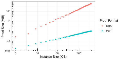
Figure 2: Proof sizes for larger Tseitin formulas using DRAT and PB proof logging.

The formulas in Table 1 contain only $50$ XOR constraints over about $100$ variables, which is very small by modern standards, and they are solved and verified in less than one second. To get a sense of the asymptotic behaviour of the proof logging, we also considered $50$ new, larger Tseitin formulas with up to $500$ XORs over up to $1250$ variables. These formulas were generated with the tool CNFgen [LENV17] using random regular graphs of degree $5$, which produces formulas with clausal encodings of $5$-XOR constraints. It was shown in [Urq87] that Tseitin formulas are hard for resolution, the reasoning method underlying conflict-driven clause learning, if the graph from which the formula is generated is an expander, and it is well known that random graphs are expanders with extremely high probability (see, e.g., [HLW06]). Thus, we can be confident that the generated formulas are hard for CDCL solvers and require additional reasoning methods, such as Gaussian elimination, to be solved efficiently.

In Figure 2 we compare the proof size for DRAT proof logging and our pseudo-Boolean VeriPB proof logging. Notice that both proof logging approaches result in straight lines in the log-log plot, which is a strong indication that they are both scaling polynomially. Studying the slopes of the lines yields the estimates that DRAT produces quadratic-size proofs while the proof size of the pseudo-Boolean proof is linear in the size of the formula. In Figure 3 we compare the running time (system time plus user time) of solving and producing the proof, as well as time spent on proof verification (where it can be noted that running times below one second should be interpreted with some care since the running time might be dominated by start-up overhead). It is clear that the larger proof size required for DRAT proofs does not only increase verification time, but also causes a clearly increased time overhead during solving.

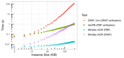
Figure 3: Solving and verification time for Tseitin formulas.

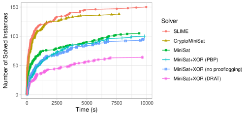
Figure 4: Cumulative plot for number of solved instances in the crypto track of the SAT Competition 2021.

To get a wider range of practically relevant formulas, we additionally evaluated our tools on cryptographic benchmarks, which often contain parity constraints, from the crypto track of the 2021 SAT competition. Figure 4 compares the performance of different solvers on this benchmark set, including SLIME [SLI], the winner of the crypto track, and CryptoMiniSat [Cry], arguably the most well-established modern solver with integrated parity reasoning. Notably, SLIME and CryptoMiniSat significantly outperform MiniSat, showing the advancements made over the last decades. Somewhat surprisingly, our integration of parity reasoning does not seem to benefit MiniSat on this set of benchmarks. However, if one insists on that the solver with parity reasoning should also support proof logging, then it is clear that more instances can be solved if we use pseudo-Boolean proof logging instead of DRAT. One reason for this is that the proof sizes are much larger when using DRAT proof logging, as shown in Figure 5. The generated DRAT proofs can quickly exceed the disk limit of roughly 100GB, causing the SAT solver to terminate with an error.

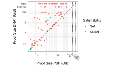
Figure 5: DRAT and PB and proof sizes for the crypto track of the SAT Competition 2021.

While the tendency of the plot in Figure 5 is clear, it should be noted that the difference shown is due not only to different proof logging methods, but also to the particular way in which we implemented proof logging for MiniSat, in which the introduction of new variables for proof logging affects the MiniSat search. This can be observed in different statistics such as the number of decisions or conflicts. For example, consider the instance in the bottom right of Figure 5 that requires a proof of a few hundred MiB in DRAT but times out for pseudo-Boolean proof logging. This instance is solved with $541,928$ conflicts with no proof logging or DRAT proof logging, but requires more than $19$ million conflicts for pseudo-Boolean proof logging. It should be emphasized, however, that this difference is completely irrelevant in that it is not in any way related to pseudo-Boolean proof logging per se, but only to a peculiar choice in the implementation we used for our experiments, as explained in the footnote above.

In Figure 6 we can see the time required for solving a benchmark versus verifying the result. In practice, it would be sufficient to only verify the final solution for satisfiable instances. However, as there are few solved unsatisfiable instances, we verified that every constraint derived by the solver is correct even for satisfiable ones. For most formulas the verification overhead is roughly a factor $10$, but there are also cases where verification is much slower, which demonstrates that further optimizations in the VeriPB proof verification code would be desirable. We are aware of several possibilities for this, such as improving RUP checks and borrowing ideas like backward trimming of proofs from DRAT-trim [DRA]. However, the main focus of this work was not on such engineering questions, but rather on developing new mathematical methods for efficient proof logging, and we would argue that the potential for vast improvements in proof logging efficiency should be clear from the experimental results reported in this section.

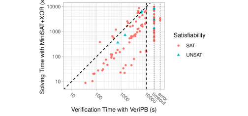
Figure 6: Time required for solving and verifying instances.

7 Conclusion

In this work, we present an efficient proof logging method for conflict-driven clause learning (CDCL) solvers equipped with parity reasoning, which has been a long-standing challenge in SAT solving. Our approach circumvents the prohibitive overhead of previous DRAT-based proof logging methods for parity reasoning such as the one developed in [PR16] by instead using the cutting planes method operating on pseudo-Boolean inequalities in the VeriPB tool [Ver] and adding a rule for introducing extension variables. An experimental evaluation shows that this makes the proof logging overhead, the size of the proof, and the time required for verification all go down by an order of magnitude or more compared to DRAT. While there is certainly ample room for further improvements, our first proof-of-concept implementation already shows the power of this approach.

In terms of weaknesses, one significant disadvantage of our method is that the proof verification time is still considerably larger than the time required for solving with proof logging, especially if many XOR constraints are involved. There are at least two explanations for this. One reason is that the algorithm for XOR reasoning can make use of bit-level parallelism. The verifier cannot do so easily, because it has to be able to deal with arbitrary linear constraints and not just XORs. Another reason is that we introduce fresh variables to encode the XOR constraints. On the solver side, these auxiliary variables can essentially be ignored, except that they are printed in fairly standardized proof logging templates, but they play a crucial role in the calculations on the proof checker side when the proof is verified. It should be said, though, that although verification overhead is larger than proof logging overhead, this is only by a constant factor. In other words, if we are willing to pay a constant-factor increase in running time, then this will allow us to not only use parity reasoning but also obtain a formal proof establishing that this parity reasoning has been performed correctly. It seems fair to argue that the benefits from fully verified solutions could outweigh the disadvantage of this limited increase in total execution time.

By construction, the pseudo-Boolean proof logging method in VeriPB can also be used to solve another task that has remained very challenging for DRAT, namely efficient proof logging for cardinality detection and reasoning. We have not investigated this in the current paper, since this is mostly an engineering question rather than a research problem in view of the methods that have already been developed in [BLLM14, EN20]. Symmetry handling, a third notorious problem for proof logging, appears to be much more difficult, but when it comes to adding symmetry breaking constraints our method can do at least as well as [HHW15], since it is a strict generalization of DRAT. In a later work [BGMN22] appearing after the conference version of this paper, the VeriPB proof logging system has been extended further with a so-called dominance-based strengthening, providing for the first time efficient proof logging support for fully general symmetry breaking. It is an interesting open question, however, whether this new dominance rule is necessary, or whether the redundance-based strengthening rule introduced in the current work is sufficient to provide efficient derivations of symmetry-breaking constraints.

The fact that no efficient proof logging support has previously been available for enhanced SAT solving techniques such as parity reasoning, cardinality detection, and symmetry handling means that SAT solvers making crucial use of such techniques have not been able to take part in the main track of the SAT competition [SAT], where proof logging is mandatory. Somewhat paradoxically, this seems to have the effect that the proof logging requirements, which have played such an important role for the development of the field, now risk becoming a barrier to further solver developments. Since the VeriPB tool can now support all of parity reasoning, cardinality detection, and (as of [BGMN22]) also symmetry breaking, and does so with very limited overhead compared to DRAT, it seems natural to propose that this should be an allowed proof logging format in future SAT competitions.

However, we believe that the potential benefit of pseudo-Boolean proof logging with extension variables goes well beyond the context of the SAT competitions. VeriPB has been shown to be capable of efficient justification of important constraint programming techniques [EGMN20, GMN22], and can also provide proof logging for a wide range of graph problem solvers [GMN20, GMM⁺20]. Furthermore, the papers [GMNO22, VWB22] have used VeriPB to develop proof logging methods that seem to have the potential to support a range of SAT-based optimization approaches using maximum satisfiability (MaxSAT) solvers. The pseudo-Boolean rules for reasoning with $0$-$1$ linear constraints provide a simple yet very expressive formalism, and it does not seem out of the question to hope that they could be extended to deal with proof logging for mixed integer programming (MIP). Thus, we believe that the ultimate goal of this line of research should be to design a unified proof logging approach for as wide as possible a range of combinatorial optimization paradigms. In addition to furnishing efficient machine-verifiable proofs of correctness, proof logging could also serve as a valuable tool for debugging and empirical performance analysis during solver development. Furthermore, the proofs produced could in principle provide auditability by third parties using independently developed software, and/or be a stepping stone towards explainability by showing, e.g., why certain solutions are optimal. We view our paper as only one of the first steps on this long but exciting road.

References

- [AAB+14] David Allouche, Isabelle André, Sophie Barbe, Jessica Davies, Simon de Givry, George Katsirelos, Barry O’Sullivan, Steve Prestwich, Thomas Schiex, and Seydou Traoré. Computational protein design as an optimization problem. Artificial Intelligence, 212(1):59–79, July 2014.
- [ABRW02] Michael Alekhnovich, Eli Ben-Sasson, Alexander A. Razborov, and Avi Wigderson. Space complexity in propositional calculus. SIAM Journal on Computing, 31(4):1184–1211, April 2002. Preliminary version in STOC ’00.
- [AGJ+18] Özgür Akgün, Ian P. Gent, Christopher Jefferson, Ian Miguel, and Peter Nightingale. Metamorphic testing of constraint solvers. In Proceedings of the 24th International Conference on Principles and Practice of Constraint Programming (CP ’18), volume 11008 of Lecture Notes in Computer Science, pages 727–736. Springer, August 2018.
- [BBH22] Randal E. Bryant, Armin Biere, and Marijn J. H. Heule. Clausal proofs for pseudo-Boolean reasoning. In Proceedings of the 28th International Conference on Tools and Algorithms for the Construction and Analysis of Systems (TACAS ’22), volume 13243 of Lecture Notes in Computer Science, pages 443–461. Springer, April 2022.
- [BCH21] Seulkee Baek, Mario Carneiro, and Marijn J. H. Heule. A flexible proof format for SAT solver-elaborator communication. In Proceedings of the 27th International Conference on Tools and Algorithms for the Construction and Analysis of Systems (TACAS ’21), volume 12651 of Lecture Notes in Computer Science, pages 59–75. Springer, March-April 2021.
- [BGMN22] Bart Bogaerts, Stephan Gocht, Ciaran McCreesh, and Jakob Nordström. Certified symmetry and dominance breaking for combinatorial optimisation. In Proceedings of the 36th AAAI Conference on Artificial Intelligence (AAAI ’22), pages 3698–3707, February 2022.
- [Bie06] Armin Biere. Tracecheck. http://fmv.jku.at/tracecheck/, 2006.
- [BLLM14] Armin Biere, Daniel Le Berre, Emmanuel Lonca, and Norbert Manthey. Detecting cardinality constraints in CNF. In Proceedings of the 17th International Conference on Theory and Applications of Satisfiability Testing (SAT ’14), volume 8561 of Lecture Notes in Computer Science, pages 285–301. Springer, July 2014.
- [BN21] Samuel R. Buss and Jakob Nordström. Proof complexity and SAT solving. In Armin Biere, Marijn J. H. Heule, Hans van Maaren, and Toby Walsh, editors, Handbook of Satisfiability, volume 336 of Frontiers in Artificial Intelligence and Applications, chapter 7, pages 233–350. IOS Press, 2nd edition, February 2021.
- [Bry22] Randal E. Bryant. TBUDDY: a proof-generating BDD package. EasyChair Preprint 8471, July 2022. Available at https://easychair.org/publications/preprint/DbRN.
- [BS97] Roberto J. Bayardo Jr. and Robert Schrag. Using CSP look-back techniques to solve real-world SAT instances. In Proceedings of the 14th National Conference on Artificial Intelligence (AAAI ’97), pages 203–208, July 1997.
- [BT19] Samuel R. Buss and Neil Thapen. DRAT proofs, propagation redundancy, and extended resolution. In Proceedings of the 22nd International Conference on Theory and Applications of Satisfiability Testing (SAT ’19), volume 11628 of Lecture Notes in Computer Science, pages 71–89. Springer, July 2019.
- [BvdKM+21] Péter Biró, Joris van de Klundert, David F. Manlove, William Pettersson, Tommy Andersson, Lisa Burnapp, Pavel Chromy, Pablo Delgado, Piotr Dworczak, Bernadette Haase, Aline Hemke, Rachel Johnson, Xenia Klimentova, Dirk Kuypers, Alessandro Nanni Costa, Bart Smeulders, Frits C. R. Spieksma, María O. Valentín, and Ana Viana. Modelling and optimisation in European kidney exchange programmes. European Journal of Operational Research, 291(2):447–456, June 2021.
- [CCT87] William Cook, Collette Rene Coullard, and György Turán. On the complexity of cutting-plane proofs. Discrete Applied Mathematics, 18(1):25–38, November 1987.
- [CEI96] Matthew Clegg, Jeffery Edmonds, and Russell Impagliazzo. Using the Groebner basis algorithm to find proofs of unsatisfiability. In Proceedings of the 28th Annual ACM Symposium on Theory of Computing (STOC ’96), pages 174–183, May 1996.
- [CFHH+17] Luís Cruz-Filipe, Marijn J. H. Heule, Warren A. Hunt, Matt Kaufmann, and Peter Schneider-Kamp. Efficient certified RAT verification. In Proceedings of the 26th International Conference on Automated Deduction (CADE-26), volume 10395 of Lecture Notes in Computer Science, pages 220–236. Springer, 2017.
- [CFMSSK17] Luís Cruz-Filipe, Joao Marques-Silva, and Peter Schneider-Kamp. Efficient certified resolution proof checking. In Proceedings of the 23rd International Conference on Tools and Algorithms for the Construction and Analysis of Systems (TACAS ’17), volume 10205 of Lecture Notes in Computer Science, pages 118–135. Springer, 2017.
- [CH20] Leroy Chew and Marijn J. H. Heule. Sorting parity encodings by reusing variables. In Proceedings of the 23rd International Conference on Theory and Applications of Satisfiability Testing (SAT ’20), volume 12178 of Lecture Notes in Computer Science, pages 1–10. Springer, July 2020.
- [CK05] Donald Chai and Andreas Kuehlmann. A fast pseudo-Boolean constraint solver. IEEE Transactions on Computer-Aided Design of Integrated Circuits and Systems, 24(3):305–317, March 2005. Preliminary version in DAC ’03.
- [CKSW13] William Cook, Thorsten Koch, Daniel E. Steffy, and Kati Wolter. A hybrid branch-and-bound approach for exact rational mixed-integer programming. Mathematical Programming Computation, 5(3):305–344, September 2013.
- [Cry] CryptoMiniSat SAT solver. https://github.com/msoos/cryptominisat/.
- [DGG+19] Maxence Delorme, Sergio García, Jacek Gondzioa, Jörg Kalcsics, David Manlove, and William Pettersson. Mathematical models for stable matching problems with ties and incomplete lists. European Journal of Operational Research, 277(2):426–441, September 2019.
- [DGP04] Heidi E. Dixon, Matthew L. Ginsberg, and Andrew J. Parkes. Generalizing Boolean satisfiability I: Background and survey of existing work. Journal of Artificial Intelligence Research, 21:193–243, 2004.
- [DRA] The DRAT format and DRAT-trim checker. https://github.com/marijnheule/drat-trim.
- [EGMN20] Jan Elffers, Stephan Gocht, Ciaran McCreesh, and Jakob Nordström. Justifying all differences using pseudo-Boolean reasoning. In Proceedings of the 34th AAAI Conference on Artificial Intelligence (AAAI ’20), pages 1486–1494, February 2020.
- [EN18] Jan Elffers and Jakob Nordström. Divide and conquer: Towards faster pseudo-Boolean solving. In Proceedings of the 27th International Joint Conference on Artificial Intelligence (IJCAI ’18), pages 1291–1299, July 2018.
- [EN20] Jan Elffers and Jakob Nordström. A cardinal improvement to pseudo-Boolean solving. In Proceedings of the 34th AAAI Conference on Artificial Intelligence (AAAI ’20), pages 1495–1503, February 2020.
- [ES04] Niklas Eén and Niklas Sörensson. An extensible SAT-solver. In 6th International Conference on Theory and Applications of Satisfiability Testing (SAT ’03), Selected Revised Papers, volume 2919 of Lecture Notes in Computer Science, pages 502–518. Springer, 2004.
- [GMM+20] Stephan Gocht, Ross McBride, Ciaran McCreesh, Jakob Nordström, Patrick Prosser, and James Trimble. Certifying solvers for clique and maximum common (connected) subgraph problems. In Proceedings of the 26th International Conference on Principles and Practice of Constraint Programming (CP ’20), volume 12333 of Lecture Notes in Computer Science, pages 338–357. Springer, September 2020.
- [GMN20] Stephan Gocht, Ciaran McCreesh, and Jakob Nordström. Subgraph isomorphism meets cutting planes: Solving with certified solutions. In Proceedings of the 29th International Joint Conference on Artificial Intelligence (IJCAI ’20), pages 1134–1140, July 2020.
- [GMN22] Stephan Gocht, Ciaran McCreesh, and Jakob Nordström. An auditable constraint programming solver. In Proceedings of the 28th International Conference on Principles and Practice of Constraint Programming (CP ’22), volume 235 of Leibniz International Proceedings in Informatics (LIPIcs), pages 25:1–25:18, August 2022.
- [GMNO22] Stephan Gocht, Ruben Martins, Jakob Nordström, and Andy Oertel. Certified CNF translations for pseudo-Boolean solving. In Proceedings of the 25th International Conference on Theory and Applications of Satisfiability Testing (SAT ’22), volume 236 of Leibniz International Proceedings in Informatics (LIPIcs), pages 16:1–16:25, August 2022.
- [GN03] Evgueni Goldberg and Yakov Novikov. Verification of proofs of unsatisfiability for CNF formulas. In Proceedings of the Conference on Design, Automation and Test in Europe (DATE ’03), pages 886–891, March 2003.
- [GN21] Stephan Gocht and Jakob Nordström. Certifying parity reasoning efficiently using pseudo-Boolean proofs. In Proceedings of the 35th AAAI Conference on Artificial Intelligence (AAAI ’21), pages 3768–3777, February 2021.
- [GNY19] Stephan Gocht, Jakob Nordström, and Amir Yehudayoff. On division versus saturation in pseudo-Boolean solving. In Proceedings of the 28th International Joint Conference on Artificial Intelligence (IJCAI ’19), pages 1711–1718, August 2019.
- [GS19] Graeme Gange and Peter Stuckey. Certifying optimality in constraint programming. Presentation at KTH Royal Institute of Technology. Slides available at https://www.kth.se/polopoly_fs/1.879851.1550484700!/CertifiedCP.pdf, February 2019.
- [GSD19] Xavier Gillard, Pierre Schaus, and Yves Deville. SolverCheck: Declarative testing of constraints. In Proceedings of the 25th International Conference on Principles and Practice of Constraint Programming (CP ’19), volume 11802 of Lecture Notes in Computer Science, pages 565–582. Springer, October 2019.
- [HHW13a] Marijn J. H. Heule, Warren A. Hunt Jr., and Nathan Wetzler. Trimming while checking clausal proofs. In Proceedings of the 13th International Conference on Formal Methods in Computer-Aided Design (FMCAD ’13), pages 181–188, October 2013.
- [HHW13b] Marijn J. H. Heule, Warren A. Hunt Jr., and Nathan Wetzler. Verifying refutations with extended resolution. In Proceedings of the 24th International Conference on Automated Deduction (CADE-24), volume 7898 of Lecture Notes in Computer Science, pages 345–359. Springer, June 2013.
- [HHW15] Marijn J. H. Heule, Warren A. Hunt Jr., and Nathan Wetzler. Expressing symmetry breaking in DRAT proofs. In Proceedings of the 25th International Conference on Automated Deduction (CADE-25), volume 9195 of Lecture Notes in Computer Science, pages 591–606. Springer, August 2015.
- [HJ12] Cheng-Shen Han and Jie-Hong Roland Jiang. When Boolean satisfiability meets Gaussian elimination in a simplex way. In Proceedings of the 24th International Conference on Computer Aided Verification, (CAV ’12), volume 7358 of Lecture Notes in Computer Science, pages 410–426. Springer, 2012.
- [HKB17] Marijn J. H. Heule, Benjamin Kiesl, and Armin Biere. Short proofs without new variables. In Proceedings of the 26th International Conference on Automated Deduction (CADE-26), volume 10395 of Lecture Notes in Computer Science, pages 130–147. Springer, August 2017.
- [HLW06] Shlomo Hoory, Nathan Linial, and Avi Wigderson. Expander graphs and their applications. Bulletin of the American Mathematical Society, 43(4):439–561, October 2006.
- [Kis] Kissat SAT solver. http://fmv.jku.at/kissat/.
- [KRH18] Benjamin Kiesl, Adrián Rebola-Pardo, and Marijn J. H. Heule. Extended resolution simulates DRAT. In Proceedings of the 9th International Joint Conference on Automated Reasoning (IJCAR ’18), volume 10900 of Lecture Notes in Computer Science, pages 516–531. Springer, 2018.
- [LENV17] Massimo Lauria, Jan Elffers, Jakob Nordström, and Marc Vinyals. CNFgen: A generator of crafted benchmarks. In Proceedings of the 20th International Conference on Theory and Applications of Satisfiability Testing (SAT ’17), volume 10491 of Lecture Notes in Computer Science, pages 464–473. Springer, August 2017.
- [LJN12a] Tero Laitinen, Tommi Junttila, and Ilkka Niemelä. Conflict-driven XOR-clause learning. In Proceedings of the 15th International Conference on Theory and Applications of Satisfiability Testing (SAT ’12), volume 7317 of Lecture Notes in Computer Science, pages 383–396. Springer, 2012.
- [LJN12b] Tero Laitinen, Tommi Junttila, and Ilkka Niemelä. Extending clause learning SAT solvers with complete parity reasoning. In Proceedings of the IEEE 24th International Conference on Tools with Artificial Intelligence (ICTAI ’12), pages 65–72, 2012.
- [LMS17] Kevin Leyton-Brown, Paul Milgrom, and Ilya Segal. Economics and computer science of a radio spectrum reallocation. Proceedings of the National Academy of Sciences, 114(28):7202–7209, July 2017.
- [LP10] Daniel Le Berre and Anne Parrain. The Sat4j library, release 2.2. Journal on Satisfiability, Boolean Modeling and Computation, 7:59–64, July 2010.
- [Man16] David F. Manlove. Hospitals/residents problem. In Ming-Yang Kao, editor, Encyclopedia of Algorithms, pages 926–930. Springer New York, 2016.
- [Min] The MiniSat page. http://minisat.se/.
- [MMNS11] Ross M. McConnell, Kurt Mehlhorn, Stefan Näher, and Pascal Schweitzer. Certifying algorithms. Computer Science Review, 5(2):119–161, May 2011.
- [MMT17] David F. Manlove, Iain McBride, and James Trimble. “Almost-stable” matchings in the hospitals / residents problem with couples. Constraints, 22(1):50–72, January 2017.
- [MMZ+01] Matthew W. Moskewicz, Conor F. Madigan, Ying Zhao, Lintao Zhang, and Sharad Malik. Chaff: Engineering an efficient SAT solver. In Proceedings of the 38th Design Automation Conference (DAC ’01), pages 530–535, June 2001.
- [MO12] David F. Manlove and Gregg O’Malley. Paired and altruistic kidney donation in the UK: Algorithms and experimentation. In Proceedings of the 11th International Symposium on Experimental Algorithms (SEA ’12), volume 7276 of Lecture Notes in Computer Science, pages 271–282. Springer, June 2012.
- [MS99] João P. Marques-Silva and Karem A. Sakallah. GRASP: A search algorithm for propositional satisfiability. IEEE Transactions on Computers, 48(5):506–521, May 1999. Preliminary version in ICCAD ’96.
- [MWB08] Martin Mann, Sebastian Will, and Rolf Backofen. CPSP-tools – Exact and complete algorithms for high-throughput 3D lattice protein studies. BMC Bioinformatics, 9:230:1–230:8, May 2008.
- [PDG13] Panos M. Pardalos, Ding-Zhu Du, and Ronald L. Graham, editors. Handbook of Combinatorial Optimization. Springer, 2nd edition, 2013.
- [PR16] Tobias Philipp and Adrián Rebola-Pardo. DRAT proofs for XOR reasoning. In Proceedings of the 15th European Conference on Logics in Artificial Intelligence (JELIA ’16), volume 10021 of Lecture Notes in Computer Science, pages 415–429. Springer, November 2016.
- [RM16] Olivier Roussel and Vasco M. Manquinho. Input/output format and solver requirements for the competitions of pseudo-Boolean solvers. Revision 2324. Available at http://www.cril.univ-artois.fr/PB16/format.pdf, January 2016.
- [SAT] The international SAT Competitions web page. http://www.satcompetition.org.
- [SAT11] SAT competition 2011: Benchmark submission guidelines. http://www.satcompetition.org/2011/format-benchmarks2011.html, 2011.
- [SB06] Carsten Sinz and Armin Biere. Extended resolution proofs for conjoining BDDs. In Proceedings of the 1st International Computer Science Symposium in Russia (CSR ’06), volume 3967 of Lecture Notes in Computer Science, pages 600–611. Springer, June 2006.
- [SB22] Mate Soos and Randal E. Bryant. Combining CDCL, Gauss-Jordan elimination, and proof generation. EasyChair Preprint 8497, July 2022. Available at https://easychair.org/publications/preprint/4rGK.
- [SGM20] Mate Soos, Stephan Gocht, and Kuldeep S. Meel. Tinted, detached, and lazy CNF-XOR solving and its applications to counting and sampling. In Proceedings of the 32nd International Conference on Computer Aided Verification (CAV ’20), volume 12224 of Lecture Notes in Computer Science, pages 463–484. Springer, July 2020.
- [SLI] SLIME: A free world class high performance SAT solver. https://maxtuno.github.io/slime-sat-solver/.
- [SNC09] Mate Soos, Karsten Nohl, and Claude Castelluccia. Extending SAT solvers to cryptographic problems. In Proceedings of the 12th International Conference on Theory and Applications of Satisfiability Testing (SAT ’09), volume 5584 of Lecture Notes in Computer Science, pages 244–257. Springer, 2009.
- [Tse68] Grigori Tseitin. On the complexity of derivation in propositional calculus. In A. O. Silenko, editor, Structures in Constructive Mathematics and Mathematical Logic, Part II, pages 115–125. Consultants Bureau, New York-London, 1968.
- [Urq87] Alasdair Urquhart. Hard examples for resolution. Journal of the ACM, 34(1):209–219, January 1987.
- [Ver] VeriPB: Verifier for pseudo-Boolean proofs. https://gitlab.com/MIAOresearch/VeriPB.
- [VS10] Michael Veksler and Ofer Strichman. A proof-producing CSP solver. In Proceedings of the 24th AAAI Conference on Artificial Intelligence (AAAI ’10), pages 204–209, July 2010.
- [VWB22] Dieter Vandesande, Wolf De Wulf, and Bart Bogaerts. QMaxSATpb: A certified MaxSAT solver. In Proceedings of the 16th International Conference on Logic Programming and Non-monotonic Reasoning (LPNMR ’22), volume 13416 of Lecture Notes in Computer Science, pages 429–442. Springer, September 2022.
- [WHH14] Nathan Wetzler, Marijn J. H. Heule, and Warren A. Hunt Jr. DRAT-trim: Efficient checking and trimming using expressive clausal proofs. In Proceedings of the 17th International Conference on Theory and Applications of Satisfiability Testing (SAT ’14), volume 8561 of Lecture Notes in Computer Science, pages 422–429. Springer, July 2014.
- [YM21] Jiong Yang and Kuldeep S. Meel. Engineering an efficient PB-XOR solver. In Proceedings of the 27th International Conference on Principles and Practice of Constraint Programming (CP ’21), volume 210 of Leibniz International Proceedings in Informatics (LIPIcs), pages 58:1–58:20, October 2021.