Slow transport and bound states for spinless fermions with long-range Coulomb interactions on one-dimensional lattices

Abstract

We study transport and relaxation of spinless fermions with long-range Coulomb interactions at high temperatures through numerical simulations of out-of-equilibrium dynamics. We find that the transport and relaxation are continuously slowing down for increasing coupling $V$, and that there is a transition in the type of transport. For intermediate couplings, the system exhibits normal diffusive transport but the time scale for the onset of that is long. For large couplings, it exhibits subdiffusive transport, while at the same time the relaxation time diverges exponentially with system lengths, featuring an MBL-like phase. We attribute the slow transport to formation of slow bound states and stable clusters of particles. For few-particle systems we prove existence, visualize the slowness and analyze collision properties of the bound states. For many particles at high densities there should be a hierarchy of clusters of particles on many different length scales. We argue that at large couplings the average maximal size of the stable clusters should scale linearly with the length of the lattice, which is in accordance with the MBL-like behavior.

I introduction

Understanding how macroscopic hydrodynamics emerges from microscopic laws is an important question, which is generally too difficult to be tractable. However, in recent years a breakthrough has been made for integrable systems, which is coined generalized hydrodynamics (GHD)[1, 2]. It has been established in GHD that integrable systems can support ballistic transport at finite temperatures due to existence of infinite many conserved charges. Various transport quantities for many 1D quantum integrable models have been calculated [3]. In particular, it has been applied to the XXZ model for its ballistic[4], diffusion [5] and superdiffusion [6, 7] regimes.

Although GHD is successful for integrable systems, integrability is rare in the real world and there are always various perturbations to break it. On the one hand, some groups have attempted to incorporate (weak) integrability breaking terms into GHD [8, 9], since one can always use the Bethe ansatz vectors as a base for generic models, being them integrable or not. On the other hand, transport of many non-integrable models has been studied numerically. These include the XXZ model with dimerization and frustration [10], staggered field [11], and spin ladders [12, 13], just to name a few. Although in the majority cases transport becomes diffusive, as it is expected, there are other cases where transport is anomalous [11, 5, 14]. Our understanding of transport of non-integrable models is still far from complete.

In the previous numerical studies, the integrability breaking terms are mostly short-ranged, and the transport quantities are extracted from dynamics in the linear response regime for relatively short time scales, so that usually normal diffusive transport is found. In this paper we study transport and relaxation of a 1D fermion model with translation invariant long-range interactions through numerical simulations of out-of-equilibrium dynamics, for longer time scales and a wide range of coupling strengths. We found that the transport and relaxation are continuously slowing down for increasing coupling $V$, and there is even a transition of the type of transport: For intermediate couplings, the relevant quantities in the dynamics would attain the values signaling normal diffusive transport or thermalization, but the processes for reaching those values are logarithmically slow in time. For large couplings, the system displays subdiffusive transport, and at the same time, the relaxation time diverges exponentially with the system sizes, showing a lack of thermalization in the thermodynamic limit.

To understand the slow transport we studied certain few-body problems of the model. We find that there are various $n$-particle bound states because of the limited band width ($\sim\lambda$) of the lattice model as well as the long-range interactions. And the group velocities of the bound states can be exponentially slow in $n$ when $V\gtrsim\lambda$. Then, for many particles with high densities and at large couplings, there should be slow moving clusters of particles on different length scales. The exponential divergence of the relaxation time is explained by possible giant immobile clusters, whose sizes may be proportional to the length of the lattice.

Several works have already discovered divergence of relaxation times in certain disorder-free models [15, 16, 17, 18, 19, 20, 21, 22, 23, 24], which was dubbed quasi-many body localization (MBL) states [20] or asymptotic localization [16, 22]. Some of these works manually introduced two components of fast and slow particles to realize such states. While we take the above point of view that there can be self-generated slow bound states or clusters [15], which is more natural and closer to realizable physical systems such as carbon nanotube or cold atom systems [25, 26]. Besides, there has been ambiguity about the nature of the quasi-MBL states [27]. We elucidate that the quasi-MBL states can be coincided with subdiffusion transport, and that a possible structure of the quasi-MBL states could be a hierarchy of stable clusters of particles but with internal resonant dynamics. Since slow bound states widely exist in quantum lattice models, we expect that they should play an important role in formulating a general theory of transport for these models, especially in the large coupling regime.

The rest of the paper is organized as follows: Sec. II introduces the model Hamiltonian and observables. Sec. III presents numerical results demonstrating the slow transport and relaxation properties. Sec. IV delivers a systematic study of the bound states of the model, including properties of their spectra, group velocities and scatterings, based on which the transport and relaxation processes are interpreted. Finally, conclusions are drawn in Sec. V.

II model and observables

The model considered here consists of a chain with $L$ sites,

$$\hat{H}= -\lambda\sum\limits_{i}{(\hat{c}_{i}^{\dagger}{{\hat{c}}_{i+1}}+h.c.)}$$ (1)

$$+\sum\limits_{i<j}{{\frac{V}{|j-i|^{\alpha}}({{\hat{n}}_{i}}-1/2)({{\hat{n}}_{j}}-1/2)}}$$

where $\hat{c}^{\dagger}_{i}$ ($\hat{c}_{i}$) is creation (annihilation) operator of a spinless fermion, and $\hat{n}_{i}$ is a fermion density operator at site $i$. The interactions decay in power laws governed by an exponent $\alpha$. This model can be rewritten via the Jordan-Wigner transformation as a quantum spin model $\hat{H}=-\frac{J}{2}\sum_{i}{(\hat{S}_{i}^{x}\hat{S}_{i+1}^{x}+\hat{S}_{i}^{y}\hat{S}_{i+1}^{y})}+\Delta\sum_{i<j}{|j-i{|^{-\alpha}}\hat{S}_{i}^{z}\hat{S}_{j}^{z}}$, after the identification of $J=2\lambda$ and $V=\Delta$. In particular, at $\alpha=\infty$, it reduces to the XXZ model (since the sign of $J$ is unimportant). By virtue of this, the languages for fermion and spin systems will be used interchangeably, and charge transport can be rephrased as spin transport. In the language of spins, the total magnetization ${\hat{S}^{z}_{\text{tot}}}=\sum_{i}{\hat{S}^{z}_{i}}$ is conserved. When there is an inhomogeneity in spin densities, spins are transported, which can be quantified by measuring the spin current operator ${\hat{j}_{i}}=J(\hat{S}_{i}^{x}\hat{S}_{i+1}^{y}-\hat{S}_{i}^{y}\hat{S}_{i+1}^{x})$.

The ground state properties of this model have been studied in Refs. [28, 29, 30, 31]. Here we investigate its transport and relaxation dynamics at high temperatures. We fix $\alpha=1$ if not otherwise specified, which corresponds to the unscreened Coulomb potential. And we focus on the range of $V\gtrsim 2$, where as we will see, the transport is slow due to formation of slow bound states. The unit $\lambda=\hbar=1$ is used, which also sets the unit of time to be $\hbar/\lambda=1$. Next we introduce two quantities to characterize transport and relaxation of the model, both of which are extracted from out-of-equilibrium dynamics.

The first quantity is a transport exponent extracted from a bipartite quench dynamics. The initial state of the dynamics is a mixed-type domain-wall state [32],

$$\rho(t=0)\propto\left(1+\mu\sigma^{z}\right)^{\otimes\frac{L}{2}}\otimes\left(1-\mu\sigma^{z}\right)^{\otimes\frac{L}{2}},$$ (2)

where $\mu$ induces an initial imbalance of magnetization between the left and right halves of the chain: $\langle\hat{S}^{z}_{i\leq L/2,i>L/2}\rangle=\pm\tfrac{1}{2}\mu$. When $\mu=0$, the system is in the maximally mixed state, corresponding to infinite temperature. A small $\mu$ will be used, which implies that the system is weakly-polarized and at a high temperature. The time evolved density matrix is given by $\rho(t)=e^{-i\hat{H}t}\rho(0)e^{i\hat{H}t}$ as usual, which can be solved numerically by using e.g. matrix product state (MPS) based algorithms (see below).

Once $\rho(t)$ is obtained, one can characterize the transport properties by the evolution of magnetization $m(i,t)=tr[\rho(t)\hat{S}^{z}_{i}]/tr[\rho(t)]$ and by the current $j_{i}(t)=tr[\rho(t)\hat{j}_{i}]/tr[\rho(t)]$. It is expected that, at large time, the magnetization will have a scaling form $m(i,t)=\varphi(\xi)$, with the scaling variable $\xi=(i-L/2)/t^{z}$, and that the current across the center cut should behave as $j_{{L/}{2}}\sim t^{z-1}$. Then the type of transport can be classified by the dynamical exponent $z$: it is ballistic if $z=1$, diffusive if $z=0.5$ and subdiffusive if $z<0.5$. In practice, $z$ is time dependent before reaching its asymptotic value, which may provide extra valuable information about the dynamics. A convenient way to extract the time dependent transport exponent is first to calculate the accumulation of spins transported through the center cut of the chain

$$\Delta M(t) =\sum_{i=1}^{L/2}{[\frac{\mu}{2}-m(i,t)]}=\sum_{i=L/2+1}^{L}{[m(i,t)+\frac{\mu}{2}]}$$

$$=\int_{0}^{t}j_{\tfrac{L}{2}}\left(t^{\prime}\right)\mathrm{d}t^{\prime}\propto t^{z},$$ (3)

and then to take a logarithmic derivative, that is

$$z(t)=d\ln(\Delta M)/d\ln(t).$$ (4)

The second quantity is extracted from the relaxation of spatial inhomogeneities of particle densities, which can be used to probe possible localized phases. Specifically, starting from an initial state $|\psi(0)\rangle$ which is a random classical state, such as $|01001\cdots 010\rangle$, its relaxation process can be measured by [19]

$$\Delta{\rho^{2}_{\psi}}(t)=\frac{1}{L}\sum\limits_{i=1}^{L}{{{\left[\langle\psi(t)|{{{\hat{n}}_{i+1}}(t)-{{\hat{n}}_{i}}(t)}|\psi(t)\rangle\right]}^{2}}},$$ (5)

where $|\psi(t)\rangle=e^{-i\hat{H}t}|\psi(0)\rangle$ is the time evolved state. Since we are interested in the dynamics at infinite temperature, an average value $\langle\Delta\rho^{2}_{\psi}(t)\rangle$ is taken for $|\psi(0)\rangle$ drawn from a sector with a fixed filling factor $\nu$ (number of particles divided by $L$). After normalizing it with its initial value, one arrives at

$$f(t)\equiv\frac{\langle\Delta\rho^{2}_{\psi}(t)\rangle}{\langle\Delta\rho^{2}_{\psi}(0)\rangle}.$$ (6)

Then one asserts that the system is localized if $f$ remains finite for infinite time, otherwise, it thermalizes.

Based on the time dependences of the two quantities $z$ and $f$, we also define two important time scales for each of them: a time scale $\tau$ for when $z$ reaches 0.5, signaling diffusive transport, and a relaxation time $\tau_{1}$ for when $f$ reaches 0, provided they do reach these values.

III numerical results

III.1 transport exponent $z(t)$

We use a two-site version of the MPS-based time dependent variation principle algorithm (TDVP) [33] to simulate the time evolved density matrix $\rho(t)$. This algorithm can deal with Hamiltonians with long-range interactions through a matrix product operator (MPO) technique [34]. The parameter $\mu$ for the initial $\rho(0)$ is set to be 0.01. The density matrix $\rho(t)$ is evaluated for $t$ up to 1000. The system size $L$ ranges from 128 to 384, depending on the coupling $V$. Larger $L$ is needed for smaller $V$, to avoid boundary effects. The largest bond dimension of the MPS used is 320.

We first show the evolution of the magnetization $m(i,t)$ for two couplings $V=4$ and $16$ in Fig. 1. Slowing down of transport with increasing $V$ can be intuitively seen from this figure. It is also due to this fact that we can simulate the quench dynamics for relatively long times with moderate costs. It is cumbersome to extract the transport exponent $z$ from the scaling form of $m(i,t)$, and even more difficult to obtain its time dependence in this way. So we extract the time dependent exponent $z(t)$ using Eqs. (II) and (4), instead.

Figure 1: Time evolution of the spin density $\mu^{-1}m(i,t)$ at $V=4$ (left panel) and $V=16$ (right panel) on a chain with $L=256$ sites. The origins of the $i$-axes are shifted to $L/2$.

Figure 2: Upper panel: dependence of the dynamical exponent $z$ on time for different coupling strengths. The inset panel shows the details at early times. The $z$ values are expected to reach 0.5 (the horizontal solid line) at large times. The dashed lines are fittings to Eq. (7). Lower panel: the time scale $\tau$ (and the fitting parameters $b$ and $k$ in the two inset panels) as a function of $V$. The values of $\tau$ are determined through Eq. (8). Symbols are data, while the solid lines are fitting functions as indicated in the legends.

The upper panel of Fig. 2 shows $z(t)$ for several intermediate coupling strengths. For each $V$ there are multiple stages in the dynamics: (i) $z$ drops from a super-ballistic value around 2 at $t\approx 0$ to around the ballistic value of 1 at $t=1$ (see the inset panel). (ii) $z$ continues dropping for $t>1$, then reaches a minimum value, and then it may fluctuate until $t=10\sim 100$, which depends on $V$. This is a transient period connecting (i) and the next stage. (iii) $z$ increases very slowly with time which can be fitted approximately by a logarithmic function

$$z(t)=k\ln(t)+b,$$ (7)

with two fitting parameters $k$ and $b$. This logarithmic process terminates when $z$ reaches 0.5. After that the system enters a steady state i.e. stage (iv). This final stage is clearly seen only for $V=2$, due to restrictions in the simulation time. But we expect that the transport should become diffusive for other values of $V$ in the figure, although the time scale $\tau$ for that to happen is much longer for larger $V$.

It is worthwhile to obtain a quantitative relationship between $\tau$ and $V$. Then a quantified value of $\tau$ is needed. To this end we use Eq. (7) and the fitting parameters $k$ and $b$ to obtain an estimated value of $\tau$, namely, by solving $z(\tau)=0.5$, which yields

$$\tau=e^{(0.5-b)/k}.$$ (8)

The result is shown in the lower panel of Fig. 2. It turns out that the estimated value of $\tau$ scales with $V$ in a power law

$$\tau\propto V^{\kappa},$$ (9)

with an exponent $\kappa\approx 3.56$. Since the dependence of $\tau$ on $V$ comes from that of $k$ and $b$ on $V$, it is beneficial to also look at the latter ones. One can see in the two inset panels that, $b$ decreases with $V$ which can be fitted in the form $b=A\ln V+B$, while $k$ seems to be a constant, these leading to a refined form of Eq. (7),

$$z(t)=k\ln(t)+A\ln V+B,$$ (10)

with the constant coefficients $k=0.023$, $A=-0.079$ and $B=0.413$.

Figure 3: Time dependence of the dynamical exponent $z$ for $V=32$. The exponent oscillates around $z=0.32$ (the red dashed line) at late times. Inset panel shows the current flowing through the center cut, which can be fitted by a power function (the red solid line) at late times.

In the above we have shown that, for intermediate couplings, the system should enter a steady state with normal diffusive transport, only that the time scale $\tau$ for the onset of it can be very long. In fact, for large couplings, the system may never reach diffusion and Eqs. (7) and (9) are no longer valid. We illustrate this in Fig. 3 for the coupling $V=32$. One can see that $z$ keeps oscillating around a constant value at late times that is below 0.5 (the oscillation may come from numerical errors when taking the logarithmic derivative in Eq. (4)). This indicates that the transport is further slowed down at large $V$ and a dynamical phase transition to subdiffusion occurs.

Note that the above quantities drawn from the bipartite quench dynamics are essentially the thermodynamic limit results. In practice we find that it is harder to simulate the dynamics for even larger $V$ using the TDVP algorithm. Next we study the other quantity $f(t)$ for short finite systems, but for much larger couplings and longer time scales.

III.2 relaxation quantity $f(t)$

We use an exact diagonalization (ED) algorithm [35] to calculate the time evolution problem $|\psi(t)\rangle=e^{-i\hat{H}t}|\psi(0)\rangle$, where periodic boundary conditions (PBC) are used. Each data of $f$ shown below are obtained by using 300 realizations of $|\psi(0)\rangle$ in the sector of $\nu=\tfrac{1}{2}$.

Figure 4: Relaxation of spatial density inhomogeneity for several pairs of coupling strengths and system sizes. Solid lines are fittings to Eq. (11).

Fig. 4 shows relaxation of the inhomogeneity $f$ for several $(L,V)$ pairs with $L\in[12,22]$ and $V\in[8,96]$, and for $t$ up to $10^{4}$. For each $(L,V)$ pair, there are multiple stages in the dynamics: (i) For $t\in[0,1]$, $f$ decays fast, whose rate depends mainly on $V$ but barely on $L$. (ii) A transient period connects (i) and the next stage. This period lasts till $t\sim O(1)$ for smaller $V$, and longer till $t\sim O(10)$ for larger $V$. (iii) A slow approximately logarithmic decay, which can be fitted by

$$f(t)=-k_{1}\ln t+b_{1},$$ (11)

with two fitting parameters $k_{1}$ and $b_{1}$. The decay rate depends mainly on $L$ but only slightly on $V$. This stage terminates, when $f$ has dropped to a low level, for example to $f\approx 0.1$ at $t\approx 80$ for $(L,V)=(18,16)$. Then the final stage (stage (iv)) starts, during which $f$ decays even slower and finally approaches zero. The final stage is only visible for small $L$ and $V$ in the figure due to limitations in the time of the simulations, but we assume that there is still such a stage for other cases. That is to say the system is expected to thermalize for all finite $L$ and $V$.

Since qualitatively the relaxation time $\tau_{1}$ for $f$ approaching 0 increases with larger $L$, an intriguing question is then: Would the relaxation time diverge in the thermodynamic limit? Then a quantitative value of $\tau_{1}$ is needed. To this end, we utilize the fitting function Eq. (11) of stage (iii) to obtain an estimated value of $\tau_{1}$ (or a lower bound of it). Namely, for each $(L,V)$ pair, it is determined by the fitting parameters,

$$\tau_{1}=e^{b_{1}/k_{1}}.$$ (12)

Then we study how this estimated relaxation time changes with $L$ and $V$.

The left panel of Fig. 5 shows dependence of $\tau_{1}$ on $L$ with fixed couplings. For small $V$, $\tau_{1}$ saturates with increasing $L$, which means that the system thermalizes in thermodynamic limit. Whereas, for each large $V$, $\tau_{1}$ grows exponentially with $L$,

$$\tau_{1}\propto e^{\sigma L},$$ (13)

with an exponent $\sigma$ possibly depending on $V$. This relation means lack of thermalization and corresponds to a quasi-MBL phase introduced in Ref. [20]. So there is a transition between the small and large coupling regimes. However, we are not meant to locate a transition point $V_{c}$ precisely in this paper. Next the dependence of $\tau_{1}$ on $V$ for each lattice size in the large coupling regime is shown in the right panel. For each $L$, $\tau_{1}$ grows with $V$ in a power law,

$$\tau_{1}\propto V^{\gamma},$$ (14)

with an exponent $\gamma$ possibly depending on $L$.

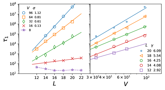
Figure 5: Left panel: dependence of relaxation time on the system size, with fixed couplings. Solid lines are fittings to Eq. (13), with the exponents $\sigma$ shown in the legend. The dashed line is a guide for the eye. Right panel: dependence of relaxation time on the coupling strength, with fixed lattice lengths. Lines are fittings to Eq. (14), with the exponents $\gamma$ shown in the legend.

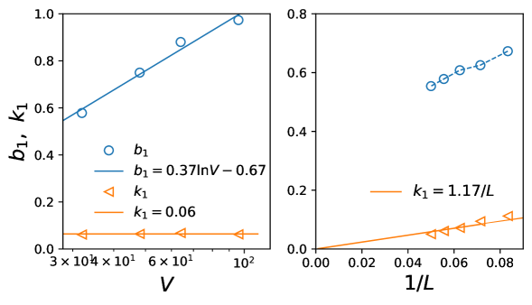
Figure 6: Dependences of the fitting parameters $b_{1}$ (symbols of circles) and $k_{1}$ (symbols of triangles) on the coupling strength $V$, for fixed $L=18$ (left panel); and dependences of them on the inverse system size $1/L$, at fixed $V=32$ (right panel). Solid lines represent fitting functions, as indicated in the legend; the dashed line is a guide for the eye.

It is tempting to obtain a full function relation $\tau_{1}(L,V)$ in the regime $V>V_{c}$. In fact, since $\tau_{1}$ is determined by the two parameters $b_{1}$ and $k_{1}$, that can be partially achieved by studying how the two parameters depend on $L$ and $V$. First we fix an $L$, say $L=18$, and look at how they depend on $V$. One can see from the left panel of Fig. 6 that $k_{1}$ obviously does not depend on $V$, while $b_{1}$ increases logarithmically with $V$. The latter can be fitted in the form $b_{1}=C\ln V+D$, where the coefficients $C$ and $D$ may be $L$-dependent. Next we fix a $V$, say $V=32$, and look at how they depend on $L$. One can see from the right panel that $k_{1}$ is proportional to the inverse system size, as $k_{1}=u/L$, where the coefficient $u\approx 1.17$ (note that $u$ should be a constant, not depending on $V$). From these, we obtain a refined form of Eq. (11)

$$f(t)=-\frac{u}{L}\ln(t)+C\ln V+D,$$ (15)

and then

$$\tau_{1}(L,V)=e^{(C\ln V+D)L/u}$$ (16)

for the regime of $V>V_{c}$.

The problem remaining is to determine the function relations $C(L)$ and $D(L)$. In fact, to make Eq. (16) consistent with Eq. (13), the only possibility is $C(L)=C_{L=\infty}+E/L+\mathcal{O}(1/L^{2})$ ($E$ being a coefficient); $D(L)$ should have a similar form for the same reason. Therefore $C$ and $D$ can be taken as constants for large $L$. We also note that, when $C\ln(V)+D=0$, $\tau_{1}$ will be finite in the thermodynamic limit. Thus this gives a way to locate the transition point by $V_{c}=\exp(-D_{L=\infty}/C_{L=\infty})$, provided the two parameters can be accurately determined. Now we make a crude approximation that taking $C$ and $D$ as constants and simply using the results at $L=18$ as their values, namely $C=0.37$ and $D=-0.67$. Then we plot the $u/L$-th root of $\tau_{1}$ versus $V$ for each $L$ in Fig. 7. The near-collapse of the data for each $L$ indicates that Eq. (16) is plausible.

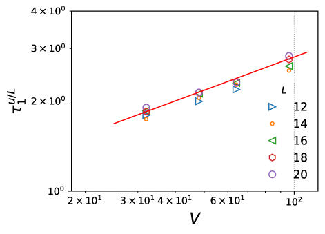
Figure 7: Rescaled relaxation time $\tau_{1}^{u/L}$ vs. the coupling strength for different system sizes. The solid line represents the function $\tau_{1}^{u/L}=e^{C\ln V+D}$, with $u=1.17$, $C=0.37$ and $D=-0.67$. The near-collapse of data to this line for each $L$ validates this function.

IV slow bound states under long-range interactions

IV.1 content of bound states

For quantum integrable systems, existence of bound states as quasi-particles is well established [36, 37]. The success of GHD just relies on identifying those quasi-particles as charge carriers. In particular, for the XXZ model a bound state is referred to as an $n$-string, which corresponds to a sequence of $n$ flipped spins (with the 1-string reduced to a single magnon). It has a group velocity $\sim\Delta^{-(n-1)}$ [38] and scatters forwardly with one another. Note that at large $\Delta$ and $n$, its velocity is so slow that it resembles a contiguous block of $n$ localized spins [39].

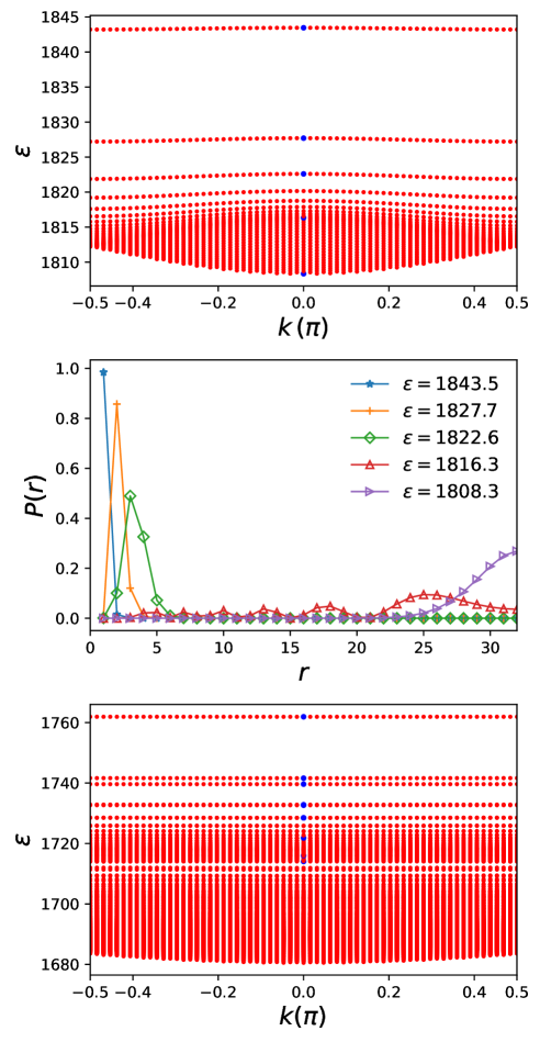
Figure 8: Top panel: 2-particle spectrum of the Hamiltonian (1) at $V=32$ on a lattice of size $L=64$. The horizontal axis represents the momentum $k$ of the states; the vertical axis represents the energy $\varepsilon$. Middle panel: distributions of two-particle separations $P(r)$ for five states in the $k=0$ sector, whose energies are shown in the legend and marked by blue dots in the top panel. Bottom panel: 3-particle spectrum for the same $V$ and $L$ as the top panel.

For generic quantum lattice models, bound states should also exist, which does not rely on integrability, but on a limited band width. We expect that they should also play an essential role in transport, especially in the strong coupling regime. For $n=2$ particles, existence of bound states can be proven for general interaction potentials, no matter they are attractive or repulsive [15, 40, 41]. For $n>2$ particles, there still lacks a general theory [15, 42, 43, 44]. However, existence of them may be anticipated from a simple energy conservation perspective: when the potential energy of a compact $n$-particle cluster is much greater than $n$ times the band width, it can’t decay into spatially far-separated smaller pieces. These arguments should also hold for lattice models with long-range interactions [41]. In the following, we show direct evidence for this for the Hamiltonian (1), by numerically diagonalizing it for a system of $n$ particles on a ring lattice, for only small $n$’s.

First the top panel of Fig. 8 shows the 2-particle spectrum on a lattice with $L=64$ sites at a coupling strength $V=32$. The few branches of energy bands on the top are bound states, while the continuum of states beneath are scattering states. To prove this, we measure the two-point correlation functions $C^{(2)}(i,j)=\langle\psi|{{\hat{n}_{i}}{\hat{n}_{j}}}|\psi\rangle$ for the eigenstates $|\psi\rangle^{\prime}s$, based on which the probability of finding the two fermions with a distance $r$ is $P(r)=\sum_{i=1}^{L}{C^{(2)}(i,i+r)}=LC^{(2)}(1,1+r)$. The second equality holds because of translation invariance. Note that all possible different $r$ values are $1,2,\dots,L/2$ on the ring lattice and $\sum_{r=1}^{r=L/2}{P(r)}=1$. Under these definitions, an eigenstate $|\psi\rangle$ should be a bound state if $P(r)$ is none-zero for only relatively small $r$, otherwise, it is a scattering state. Here we show $P(r)$ in the middle panel of Fig. 8 for only five representative states, which are all in the zero momentum sector and indicated by blue dots in the top panel. For the first three states in the top bands, $P(r)$ has pronounced peaks at $r=1,2$ and $3$, respectively, while being depressed for large $r$. This shows that they are all bound states, and that the main contributions in the two-particle configurations are, respectively, “11”, “101” and “1001” (here 1 represents an occupied site, 0 for an empty site, and trailing 0’s are omitted for clarity). In contrast, for the two states in the continuum region, $P(r)$ is none-zero for a wide range of $r$, so they are scattering states.

Table 1: An (incomplete) list of 3-particle bound states in the zero momentum sector. The four columns from left to right are: state numbers (numbered from highest to lowest energy in that sector), energies ($\varepsilon$) of the states, strings ($s$) representing particle configurations and the probabilities for each configurations $P(s)$, respectively. For each state, only configurations whose probability is larger than 0.4 are listed.

state number	$\varepsilon$	$s$	$P(s)$
#1	$1761.92$	111	0.996
#2	$1741.61$	1011	0.494
		1101	0.494
#3	$1739.64$	1101	0.487
		1011	0.487
#4	$1732.83$	11001	0.461
		10011	0.461
#5	$1732.66$	10011	0.469
		11001	0.469
#6	$1728.49$	110001	0.416
		100011	0.416
#7	$1728.49$	100011	0.418
		110001	0.418
#14	$1721.82$	10101	0.941
#52	$1716.00$	101001	0.470
		100101	0.470
#64	$1714.07$	100101	0.423
		101001	0.423

Next we consider the system with three fermions. Three-particle states are more cumbersome to characterize, for which the three-point correlation functions $C^{(3)}(i,j,k)=\langle\psi|{\hat{n}_{i}}{\hat{n}_{j}}{\hat{n}_{k}}|\psi\rangle$ are needed. Besides that, we introduce some notations and terminologies for better describing these states. We still use strings made up of 1’s and 0’s to denote particle configurations (up to translations on the ring lattice): “111” means they occupy three contiguous sites; “1101” means two of them are nearest-neighbored and the other one is to the right of them but separated by 1 site, and so forth. Then the probability $P(s)$ for a configuration $s$ found in a state $|\psi\rangle$ is determined by the three-point function, for example, $P(\text{``111''})=LC^{(3)}(1,2,3)$ and $P(\text{``1101''})=LC^{(3)}(1,2,4)$. A configuration with a significant probability will be called as a primary configuration. Two configurations which are energetically equivalent, e.g. “1101” and “1011”, are called resonant configurations [19, 16].

The three-fermion spectrum is shown in the bottom panel of Fig. 8, where the system parameters are the same as the case of $n=2$. It suffices to consider only the zero momentum sector, because the contents of bound states in different sectors will be similar. There are 561 states in all in that sector. For each state, we have measured the probability of occurrence of every configuration. Table 1 lists only the primary configurations for certain states, which are marked by blue dots in the bottom panel: For the 1st state at $\varepsilon=1761.92$, there is only one primary configuration, with its probability equal to 0.996. For the 2nd state at $\varepsilon=1741.61$, there are two primary configurations “1101” and “1011”, which are in resonance, and their probabilities are both equal to 0.494. The 3rd state at $\varepsilon=1739.63$ is nearly degenerate with the 2nd state. It has the same primary configurations as the former, only that the probability goes down slightly to 0.487. As a matter of fact, the main difference between the 2nd state and the 3rd state is that the former is of odd parity while the latter is of even parity. Likewise, the 4th and 5th states are nearly degenerate and have the same primary configurations, but differ in parities. It is easy to see that these states are all bound states, so should be the rest states in the table.

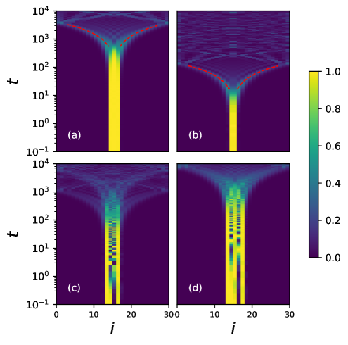
Figure 9: Time evolution of localized blocks of particles. The initial states are product states $|0\dots 0s0\dots 0\rangle$, where $s$ for (a)-(d) are “111”, “11”, “1101” and “11101”, respectively. The time evolution is obtained by using ED with PBC; the system sizes are all $L=30$ and the coupling strengths $V=32$; the color map encodes densities of particles. In (a) and (b), the dashed lines are fittings of the peak positions of the densities in the wave fronts to a linear function $i=\pm v_{\text{g,max}}t+const.$, with $v_{\text{g,max}}$ being 1/247.3 and 1/8.7 respectively.

From the above results we see that not only do bound states exist under long-range interactions, but their types are much richer than that of the short-ranged XXZ model. We will not study the general cases of $n>3$, but one may appreciate that at large couplings for every compact particle configuration (up to resonances) there should be a corresponding bound state. We also note that in an $n$-particle spectrum the high energy states are bound states, while the states in the bottom are scattering states (in the middle the states hybridize bound states and scattering states). The high energy bound states move slowly, while the latter move fast. Details of this point are explained in the next subsection.

IV.2 velocities of bound states, and duality between bound states and localized particle blocks

The single-particle states (singletons, or magnons in the language of spins) have the dispersion $\varepsilon(k)=-2\cos(k)$. Therefore the maximal value of their group velocities, denoted by $v_{\text{g,max}}$, equals $2$, which does not depend on the coupling strength. For bound states with $n\geq 2$, their maximal group velocities loosely speaking behave like

$$v_{\text{g,max}}\sim V^{-(n-1)}$$ (17)

in $n$-th order of perturbation theory, so they can be very slow at large $V$ or $n$. And $n$ can be seen as an effective mass of a quasi-particle. A more concrete and precise form of $v_{\text{g,max}}$ should nevertheless depend also on the primary configurations of the bound states. In particular, when a primary configuration is resonant, there can be internal dynamics, which will be made clearer in the following discussions.

At large couplings, there is one kind of duality between $n$-particle bound states and localized $n$-particle blocks when they have corresponding configurations. By duality we mean that they are connected approximately by Fourier transformation, as they are respectively eigenstates of momentum and position operators, and the connection is sharpened with increasing $V$. This can be seen as a generalisation for that of the XXZ model [45, 38, 39]. Based on the duality one may visualize the motion of the bound states by looking at evolution of corresponding localized blocks. Here time evolution of four simplest configurations at $V=32$ is illustrated in Fig. 9. Each of the four blocks delocalizes with time due to moving of its dual bound states and other states (contributions from the other states are however negligibly small at large $V$). The wave fronts of the fastest modes form linear light cones, which can be clearly seen for the two non-resonant configurations “111” and “11” (see subplots (a) and (b)). The $v_{\text{g,max}}$ of them can be determined by measuring the slopes of the light cones, which are 1/247.3 and 1/8.7 respectively, differing by a factor about $V$ and in agreement with Eq. (17). The other two configurations “1101” and “11101” are both resonant, whose time evolution is a bit more complicated (see subplots (c) and (d)). As a whole, they also move slowly, but they can contain faster internal dynamics. The two resonant configurations are of first and second order, respectively. Here the order $p$ of a resonant configuration is defined as the number of displacements required to change it to its resonant counterpart [19]. Then quantitatively the speed of the internal particles in it should scale as $\sim V^{-(p-1)}$. In particular, the central particle in the first-order resonance has a velocity $\approx 1.5$, which is fast and does not depend on $V$.

Note that the duality approximately holds for only large $V$. When $V$ is reduced, a localized $n$-particle block will receive more and more contributions from lighter and faster $m$-particle states, for all $m<n$. This is similar to the results of the XXZ model [45], and we will not show numerical evidence for this for the present model. So delocalization of a block of localized particles is quickened by a smaller $V$ for dual reasons: it is decomposed more into lighter types of quasi-particles, and the velocities of each type of quasi-particles scale faster (through Eq. (17)). This point is crucial for understanding the result in the last section that a thermalization to quasi-MBL transition occurs when varying $V$.

IV.3 interpretations of the relaxation processes

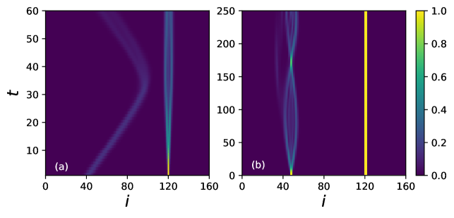
Figure 10: Collisions between quasi-particle wave packets: Panel (a) depicts a Gaussian wave packet of a singleton colliding with 2-particle wave packets, the latter being decomposed from a localized 2-particle block. Panel (b) shows evolution of two initially localized blocks “11” and “111” with a separation of 70 lattice sites. The dynamics are obtained by using TDVP for $V=32$, $L=160$ and PBC. The color map encodes densities of particles.

At a large coupling the only fast modes are the singletons and the first-order resonant processes, while other modes are all slow and differ in orders of magnitude of $V$. Given existence of slow quasi-particles, to account for the macroscopic transport and relaxation processes, one still needs to know how these quasi-particles interact with one another, which we discuss next. The discussions are first restricted to the large coupling regime, where the physical picture is simpler and the above-stated duality can be utilized. Depending on the density of particles on the lattice, the physical pictures can be very different.

For very low particle densities the physical picture is this: far apart quasi-particles are moving on the lattice, and faster ones are jammed by slower ones. We illustrate this point by two examples of few-body dynamics. The first example is a right-moving Gaussian wave packet of a singleton colliding with a 2-particle wave packet, the latter being decomposed from a localized 2-particle block (the detailed definition of the initial state is given in the appendix). It turns out that they are backscattered before approaching very close to each other, as shown in Fig. 10(a). This is in stark contrast with the XXZ model [46, 45], where the nearest-neighbor interactions lead to only forward scatterings. The second example is a 2-particle block interacting with a 3-particle block. The quasi-particles decomposed from the 2-particle block are also backscattered by the more stable 3-particle block, so that the motion of the former is constrained (see Fig. 10(b)). From these two simple examples, we infer that two quasi-particles of general types may be always backscattered by each other under the long-range Coulomb potentials, provided they are initially far apart. We will however not delve deeper for the low particle densities, as the macroscopic relaxation processes presented in section III.2 are at half filling, which is discussed next.

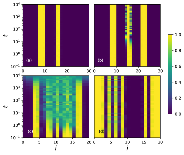
Figure 11: Time evolution for certain product state initial states: For subplots (a) and (b) the particle configurations are “1110000011” and “11100000110000111”, respectively, both on a lattice with 30 sites. For (c) and (d) both are 10 particles on a lattice with 20 sites, where the initial particle configurations can be read off from the graphs. The color map encodes densities of particles. The dynamics are obtained by using ED with PBC; the coupling strength $V=32$ for all cases.

At or close to half filling, the crowdedness of the particles leads to two competing effects. On the one hand, it reinforces the stability of small particle blocks and localizes the particles. For example when two localized blocks “111” and “11” are placed nearby, say five sites away, the stability of them are both reinforced (see Fig. 11(a)). This can potentially lead to a large and stable cluster, when more particles are added nearby. But on the other hand, the crowdedness also leads to numerous resonant configurations, that tend to delocalize certain particles. For example if another “111” block is added to four sites to the right of the previous 5-particle system, then the two fermions in the middle move faster due to resonance (see Fig. 11(b)). We note that the former effect dominates at large length scales, whereby large and stable clusters may form; while the latter is constrained to be in small length scales, inside the clusters; but eventually the clusters thermalize locally through the resonances.

The time scales for local thermalization of the clusters vary significantly, which depend on specific configurations. For example comparing the two configurations of Fig. 11(c) and (d), both being a cluster of 10 particles on a lattice with 20 sites, the former thermalizes faster than the latter. Usually, for a given coupling strength, the clusters with high energy densities (i.e. containing long contiguously occupied sites) or containing resonances at only high orders thermalize slower. Now imagine a system with more particles on a larger lattice than the examples of (c) and (d). Then in some regions the clusters will thermalize fast and in some other regions they do so slowly. While the point is that the motion of the thermalized (or “delocalized”) regions is still constrained by surrounding more stable clusters, which prevents the entire system from thermalizing. In other words, local thermalization can be embedded in global quasi-localization. One may continue this thought and consider the system just stated to be on an even larger lattice, and on and on. These descriptions would in the end lead to the picture of a hierarchy of stable clusters of particles on many different length scales.

Each length scale $\ell$ of the stable clusters determines a local thermalization time scale. While the most important is the one with the maximal size $\ell_{max}$, which determines the relaxation time of the entire system. For a system described by an ensemble at a certain high temperature, the relevant quantity is an ensemble-averaged value $\langle\ell_{max}\rangle$. We expect that when $V$ is large, this value should be proportional to the system length, $\langle\ell_{max}\rangle\propto L$, so that this together with Eq. (17) is roughly in accordance with the exponential scaling of $\tau_{1}$ with $L$ and the power-law scaling of it with $V$ (i.e. Eqs. (13) and (14)). As $V$ decreases, the clusters of particles are less stable due to the reasons stated in the final paragraph of the last subsection. Then we expect that when $V$ is smaller than some threshold, $\langle\ell_{max}\rangle$ should saturate as $L$ increases, and the stable clusters are all relatively small-sized. So these arguments provide a microscopic mechanism for the quasi-MBL to thermalization transition.

No matter the average maximal size of the stable clusters grows linearly with $L$ or not, for any finite $L$, clusters on all length scales will gradually delocalize, starting from the lowest-order resonances. The intermediate time scales in the transport and relaxation processes are related to different sizes of clusters (quasi-particles) and different orders of resonances. Specifically, the fast decay of $f$ for $t\leq 1$ (i.e. stage (i)) is completely due to motion of the first-order resonances and the singletons. The velocities of these fast modes do not depend on $V$, but the densities of them do, that is why $f$ drops to lower values for smaller $V$. These facts are also consistent with $z\approx 1$ at $t=1$. The transient periods (stages (ii)) for both $f(t)$ and $z(t)$ should be because of further relaxations related to these fast modes. The slow change of $f$ and $z$ with time in stages (iii) should be caused by successive relaxation of each intermediate-sized clusters, through each higher order resonances. However, a quantitative explanation of why they are approximately in logarithmic forms needs further investigation.

V conclusion

We studied transport and relaxation of the fermion model with long-range Coulomb interactions for a wide range of couplings. By extracting two time-dependent quantities $z(t)$ and $f(t)$ from out-of-equilibrium dynamics, we showed that when tuning the coupling strength of the long-range interactions, there is a dynamical phase transition at high temperatures. For large couplings, the system exhibits anomalous subdiffusive transport (through the behavior of $z$) and at the same time quasi-localization (through $f$), whereby a correspondence between the two descriptions is established. For intermediate couplings, the system exhibits normal diffusive transport and thermalization after certain time scales. However, even in this “normal” regime, both $z$ and $f$ change slowly with time before reaching those time scales, which can be fitted by logarithmic functions. This shows that the usual assumption of rapid local chaotic thermalization of Hydrodynamics is false for the present non-integrable model.

We have tried to interpret the macroscopic transport and relaxation processes by studying few-particle problems on the lattice. We found that there is a richness of types of bound states under the long-range Coulomb force. And the motion of all quasi-particles all slow down except the singletons and first-order resonances, when the coupling strength increases. Besides, for many particles at large densities, the long-range interactions tend to bind localized blocks together to form large clusters, but at the same time, they also lead to various internal resonant processes. In the end there should be a hierarchy of clusters on different length scales. We argue that at large couplings there should be giant immobile clusters, which gives an interpretation of the structure of the quasi-MBL states.

Every quantum lattice model, being it integrable or not, should be able to produce bound states, and the bound states are slow moving. But not every model supports slow transport at large couplings and high temperatures. Another decisive factor yet required is formation of large and stable clusters of particles. This depends on specific forms of interactions. It appears that long-range power-law interactions usually suffice for this requirement, since where slow relaxation dynamics are found in the present model and in previous works [15, 19, 24]. Nevertheless, we expect that similar slow transport may be found in a much wider range of models. It is interesting to determine the minimal conditions for the slow dynamics in future works.

*

Appendix A initial state for the collision dynamics

Following Refs. [46] and [47], the initial state $|\psi(0)\rangle$ of the dynamics is created by acting the operator (up to normalization)

$$\sum\limits_{x}{\exp}\left({-\frac{{{{\left({x-{x_{0}}}\right)}^{2}}}}{{2{\sigma^{2}}}}}\right)\exp\left({i\left({x-{x_{0}}}\right){k_{0}}}\right)c_{x}^{\dagger}$$ (18)

on a product state $|0\dots 0110\dots 0\rangle$ for a block of two localized particles. This operator creates a right-going Gaussian wave packet with momentum $k_{0}=-\pi/2$, width $\sigma=4$, and center position $x_{0}$ as depicted in the figure.

References

References

- Bertini et al. [2016] B. Bertini, M. Collura, J. De Nardis, and M. Fagotti, Phys. Rev. Lett. 117, 207201 (2016).
- Castro-Alvaredo et al. [2016] O. A. Castro-Alvaredo, B. Doyon, and T. Yoshimura, Phys. Rev. X 6, 041065 (2016).
- Bertini et al. [2021] B. Bertini, F. Heidrich-Meisner, C. Karrasch, T. Prosen, R. Steinigeweg, and M. Žnidarič, Rev. Mod. Phys. 93, 025003 (2021).
- Ilievski and De Nardis [2017] E. Ilievski and J. De Nardis, Phys. Rev. Lett. 119, 020602 (2017).
- De Nardis et al. [2019] J. De Nardis, D. Bernard, and B. Doyon, SciPost Phys. 6, 049 (2019).
- Ljubotina et al. [2019] M. Ljubotina, M. Žnidarič, and T. Prosen, Phys. Rev. Lett. 122, 210602 (2019).
- Gopalakrishnan and Vasseur [2019] S. Gopalakrishnan and R. Vasseur, Phys. Rev. Lett. 122, 127202 (2019).
- Friedman et al. [2020] A. J. Friedman, S. Gopalakrishnan, and R. Vasseur, Phys. Rev. B 101, 180302(R) (2020).
- Bastianello et al. [2021] A. Bastianello, A. D. Luca, and R. Vasseur, J. Stat. Mech.: Theory Exp. 2021 (11), 114003.
- Langer et al. [2009] S. Langer, F. Heidrich-Meisner, J. Gemmer, I. P. McCulloch, and U. Schollwöck, Phys. Rev. B 79, 214409 (2009).
- Bulchandani et al. [2020] V. B. Bulchandani, C. Karrasch, and J. E. Moore, PNAS 117, 12713 (2020).
- Zotos [2004] X. Zotos, Phys. Rev. Lett. 92, 067202 (2004).
- Jung et al. [2006] P. Jung, R. W. Helmes, and A. Rosch, Phys. Rev. Lett. 96, 067202 (2006).
- Chen et al. [2023] C. Chen, Y. Chen, and X. Wang, Superdiffusive to Ballistic Transports in Nonintegrable Rydberg Chains (2023), arXiv:2304.05553 [cond-mat].
- Kagan and Maksimov [1984] Y. Kagan and L. A. Maksimov, J. Exp. Theor. Phys. 60, 201 (1984).
- De Roeck and Huveneers [2014] W. De Roeck and F. Huveneers, Commun. Math. Phys. 332, 1017 (2014).
- Grover and Fisher [2014] T. Grover and M. P. A. Fisher, J. Stat. Mech. 2014, P10010 (2014).
- Schiulaz and Müller [2014] M. Schiulaz and M. Müller, AIP Conf. Proc. 1610, 11 (2014).
- Schiulaz et al. [2015] M. Schiulaz, A. Silva, and M. Müller, Phys. Rev. B 91, 184202 (2015).
- Yao et al. [2016] N. Yao, C. Laumann, J. Cirac, M. Lukin, and J. Moore, Phys. Rev. Lett. 117, 240601 (2016).
- Mondaini and Cai [2017] R. Mondaini and Z. Cai, Phys. Rev. B 96, 035153 (2017).
- Bols and De Roeck [2018] A. Bols and W. De Roeck, J. Math. Phys. 59, 021901 (2018).
- Michailidis et al. [2018] A. A. Michailidis, M. Žnidarič, M. Medvedyeva, D. A. Abanin, T. Prosen, and Z. Papić, Phys. Rev. B 97, 104307 (2018).
- Spielman et al. [2022] S. E. Spielman, A. Handian, N. P. Inman, T. J. Carroll, and M. W. Noel, Slow Thermalization of Few-Body Dipole-Dipole Interactions (2022), arXiv:2208.02909 [quant-ph].
- Baumann et al. [2010] K. Baumann, C. Guerlin, F. Brennecke, and T. Esslinger, Nature 464, 1301 (2010).
- Landig et al. [2016] R. Landig, L. Hruby, N. Dogra, M. Landini, R. Mottl, T. Donner, and T. Esslinger, Nature 532, 476 (2016).
- Papic et al. [2015] Z. Papic, E. M. Stoudenmire, and D. A. Abanin, Ann Phys-new York 362, 714 (2015).
- Capponi et al. [2000] S. Capponi, D. Poilblanc, and T. Giamarchi, Phys. Rev. B 61, 13410 (2000).
- Hohenadler et al. [2012] M. Hohenadler, S. Wessel, M. Daghofer, and F. F. Assaad, Phys. Rev. B 85, 195115 (2012).
- Li [2019] Z.-H. Li, J. Phys.: Condens. Matter 31, 255601 (2019).
- Ren et al. [2020] J. Ren, W.-L. You, and X. Wang, Phys. Rev. B 101, 094410 (2020).
- Ljubotina et al. [2017] M. Ljubotina, M. Žnidarič, and T. Prosen, Nat Commun 8, 16117 (2017).
- Haegeman et al. [2016] J. Haegeman, C. Lubich, I. Oseledets, B. Vandereycken, and F. Verstraete, Phys. Rev. B 94, 165116 (2016).
- Crosswhite et al. [2008] G. M. Crosswhite, A. C. Doherty, and G. Vidal, Phys. Rev. B 78, 035116 (2008).
- Weinberg and Bukov [2017] P. Weinberg and M. Bukov, SciPost Phys. 2, 003 (2017).
- Bethe [1931] H. Bethe, Z. Physik 71, 205 (1931).
- Takahashi [1999] M. Takahashi, Thermodynamics of One-Dimensional Solvable Models (Cambridge University Press, 1999).
- Wöllert and Honecker [2012] A. Wöllert and A. Honecker, Phys. Rev. B 85, 184433 (2012).
- Mossel and Caux [2010] J. Mossel and J.-S. Caux, New J. Phys. 12, 055028 (2010).
- Winkler et al. [2006] K. Winkler, G. Thalhammer, F. Lang, R. Grimm, J. Hecker Denschlag, A. J. Daley, A. Kantian, H. P. Büchler, and P. Zoller, Nature 441, 853 (2006).
- Valiente [2010] M. Valiente, Phys. Rev. A 81, 042102 (2010).
- Mattis [1986] D. C. Mattis, Rev. Mod. Phys. 58, 361 (1986).
- Valiente et al. [2010] M. Valiente, D. Petrosyan, and A. Saenz, Phys. Rev. A 81, 011601 (2010).
- Kornilovitch [2013] P. E. Kornilovitch, EPL 103, 27005 (2013).
- Vlijm et al. [2015] R. Vlijm, M. Ganahl, D. Fioretto, M. Brockmann, M. Haque, H. G. Evertz, and J.-S. Caux, Phys. Rev. B 92, 214427 (2015).
- Ganahl et al. [2013] M. Ganahl, M. Haque, and H. G. Evertz, arXiv preprint arXiv:1302.2667 (2013).
- Ulbricht and Schmitteckert [2009] T. Ulbricht and P. Schmitteckert, EPL 86, 57006 (2009).