A dynamically discovered and characterized non-accreting neutron star - M dwarf binary candidate

Abstract

Optical time-domain surveys can unveil and characterize exciting but less-explored non-accreting and/or non-beaming neutron stars (NS) in binaries. Here we report the discovery of such a NS candidate using the LAMOST spectroscopic survey. The candidate, designated LAMOST J112306.9+400736 (hereafter J1123), is in a single-lined spectroscopic binary containing an optically visible M star. The star’s large radial velocity variation and ellipsoidal variations indicate a relatively massive unseen companion. Utilizing follow-up spectroscopy from the Palomar 200-inch telescope and high-precision photometry from TESS, we measure a companion mass of $1.24_{-0.03}^{+0.03}~{}M_{\odot}$. Main-sequence stars with this mass are ruled out, leaving a NS or a massive white dwarf (WD). Although a massive WD cannot be ruled out, the lack of UV excess radiation from the companion supports the NS hypothesis. Deep radio observations with FAST yielded no detections of either pulsed or persistent emission. J1123 is not detected in numerous X-ray and gamma-ray surveys. These non-detections suggest that the NS candidate is not presently accreting and pulsing. Our work exemplifies the capability of discovering compact objects in non-accreting close binaries by synergizing the optical time-domain spectroscopy and high-cadence photometry.

Department of Astronomy, Xiamen University, Xiamen, Fujian 361005, P. R. China

National Astronomical Observatories, Chinese Academy of Sciences, Beijing 100101, P. R. China

Department of Physics and Astronomy, University of California, 1 Shields Avenue, Davis, CA 95616-5270, USA

Department of Astronomy, Nanjing University, Nanjing 210046, P. R. China

Yunnan Observatories, Chinese Academy of Sciences, Kunming 650216, P. R. China

South-Western Institute for Astronomy Research, Yunnan University, Kunming 650500, P. R. China

Department of Astronomy, Beijing Normal University, Beijing 100875, P. R. China

International Laboratory for Quantum Functional Materials of Henan, and School of Physics and Microelectronics, Zhengzhou University, Zhengzhou, Henan 450001, P. R. China

School of Astronomy and Space Science, University of Chinese Academy of Sciences, Beijing 100049, P. R. China

Department of Physics, Xiamen University, Xiamen, Fujian 361005, P. R. China

The demographic and physical properties (e.g., birth rates and mass distributions[1]) of NSs hold essential information about the stellar evolution and chemical enrichment history of our Galaxy. NSs are typically discovered with different manifestations[2] in the electromagnetic window, e.g., rapidly rotating and highly magnetized radio pulsars[3], accreting NS X-ray binaries, gamma-ray pulsars[4], and nearby isolated thermally emitting NSs[5]. In recent years, coalescing NSs that produce gravitational waves[6] have also been detected by LIGO and Virgo. However, samples of currently discovered NSs are far from being complete and representative. Since radio, X-ray, or gamma-ray observations discover NSs only if they are beaming towards us or the NS is accreting material from its companion, the population of non-accreting and/or radio quiet NSs[7] remains largely undetected.

In the optical window, large spectroscopic surveys like LAMOST[8, 9] (Large Sky Area Multi-Object Fiber Spectroscopic Telescope) have been monitoring millions of stars and archiving the largest spectroscopic database. By mining the wealth of large spectroscopic databases, one can implement the radial velocity (RV) method to discover systems that harbor a hidden compact object in orbiting with a luminous stellar companion[10], e.g., stellar-mass black holes (BH). A handful of notable systems have been discovered recently, such as MWC 656[11], LB-1[12], and J05215658+4359220[13]. These BHs reside in wide binaries with an orbital period typically $\gtrsim$ 50 days. By synergizing multi-epoch spectroscopic and photometric surveys, one can dynamically measure their masses. In principle, searching for NSs using this methodology would be feasible. Surprisingly, only two potential candidates have been discovered by the dynamical method to date, i.e., J05215658+4359220[13] and V723 Mon[14]. While each system might contain a massive NS, a non-interacting, mass-gap[15] BH ($\sim$ 3 $M_{\odot}$) was considered more likely.

Here we report the discovery of a close binary system with a non-accreting NS candidate. This system, designated LAMOST J112306.9+400736 (hereafter J1123), is a single-lined spectroscopic binary with an early-type M dwarf at a distance of 318 pc. On February 22, 2015, the M-star showed a radial velocity change of $\sim$ 270 km s^-1 within $\sim$ 68 minutes. Such a large and rapid velocity shift and the characteristic ellipsoidal variations[16] showing on multi-band light curves (Figure 1; lower panels) indicate a relatively massive unseen companion. Archival data and follow-up observations confirm the presence of a compact companion, which is either a NS or a massive and cold white dwarf (WD).

1 Results

Following the discovery of J1123, we took follow-up spectroscopy by using the Double Spectrograph (DBSP) mounted on Palomar’s 200-inch telescope (P200), to obtain ten more exposures (Figure 1; upper panel). Utilizing the multi-epoch spectroscopy and photometry, we measure the dynamical mass of the unseen companion to be $1.24_{-0.03}^{+0.03}~{}M_{\odot}$. Because normal stars with similar masses would easily outshine the visible M dwarf, we conclude that the unseen component must be a compact object. Supplementary Table 1 summarizes the stellar and binary parameters of J1123.

1.1 The orbital ephemeris, radial velocity curve, and the mass function

The orbital ephemeris of J1123 is:

$$T(\phi=0)=2\,453\,734.909\,32(31)\mathrm{HJD}+0.273\,835\,44(18)\times N\ ,$$ (1)

where the first term in the right hand is an epoch of the superior conjunction (denoted as $T_{0}$, i.e., corresponding to phase $\phi$ $=$ 0 where the M dwarf is farthest away from the observer), HJD is the Heliocentric Julian Date, and the second term is the orbital period times the number of orbital cycles $N$ (see Methods). Last two digits inside the parenthesis indicate the one-sigma uncertainties.

We measure the RVs by cross-correlating the spectra to a library of empirical spectra[17] (see Methods). Both RVs and photometric data are phase-folded according to Equation (1). We assume that the orbit is circularized and use a sinusoidal curve $V_{\mathrm{R}}=-K_{1}\sin(2\pi(t-T_{0})/P_{\mathrm{orb}})+\gamma$ to fit the RV data (Figure 1), where $K_{1}$ is the RV curve semi-amplitude, $t$ is the mid-time of each exposure, $P_{\rm orb}$ is the orbital period, and $\gamma$ is the systemic velocity. The fitting results in $K_{1}$ $=$ 257 $\pm$ 2 km s^-1 and $\gamma$ $=$ $-$8 $\pm$ 2 km s^-1. Hence the mass function (lower mass limit) for the invisible companion is:

$$f(M_{\rm 2})=\frac{M_{2}^{3}\sin^{3}(i)}{(M_{1}+M_{2})^{2}}=\frac{K_{1}^{3}P_{\rm orb}}{2\pi G}=0.48\pm 0.01~{}M_{\odot}\ ,$$ (2)

where $M_{1}$ and $M_{2}$ are the masses of the visible and invisible components, respectively, $i$ is the orbital inclination, and $G$ is the gravitational constant.

1.2 The stellar properties of the M dwarf

The visible star has a spectral type of M1, featuring the TiO molecular absorption bands of a typical M dwarf. Emission lines of Ca II H&K and Balmer series (H$\alpha$ – H$\gamma$) are presented in all of J1123’s spectra. We found that these emission lines are co-moving with the M dwarf, suggesting that they originate from the hot chromosphere of the M dwarf (see Methods).

We fit the broadband SED (Figure 2) of J1123 using its archival photometry and utilizing the distance $D=318\pm 4$ pc derived from the parallax $\bar{\omega}$ $=$ 3.147 $\pm$ 0.038 mas (Gaia EDR3[18]). The best-fit model SED has an effective temperature $T_{\mathrm{eff,1}}$ $=$ 3769${}_{-9}^{+8}$ K, a radius $R_{1}$ $=$ 0.63 $\pm$ 0.01 $R_{\odot}$, and a bolometric luminosity $L_{\mathrm{bol}}$ $=$ 4 $\pi R_{1}^{2}\sigma T_{\mathrm{eff,1}}^{4}$ $=$ 0.071 $\pm$ 0.002$L_{\odot}$. We measure a stellar mass $M_{1}$ $=$ 0.61 $\pm$ 0.02 $M_{\odot}$ of the M dwarf by fitting the stellar model isochrones (see Methods).

1.3 The orbital solution: unveiling the nature of the invisible

Equipped with all the observed and derived properties of the visible M dwarf, we model the RV curve and the ellipsoidal light curve using the PHOEBE software and solve: the orbital inclination $i$, the mass ratio $q\,(\equiv M_{2}/M_{1})$, and hence the compact object’s mass $M_{2}$. By fixing $M_{1}=0.61\ M_{\odot}$ and $R_{1}=0.63\ R_{\odot}$, we obtain the following orbital solution (for a complete discussion, see Methods): $i=73^{+1.8}_{-1.5}$ degree and $M_{2}=1.24_{-0.03}^{+0.03}~{}M_{\odot}$ (Figure 3). The measured mass suggests that the compact object is either a massive WD or a NS.

We present evidence against a WD. From the spectroscopic point of view, there are no broad absorption features of a WD detected in the vicinity of the Balmer lines, and the P200 spectra are well fitted with the M dwarf template (see Methods). From the photometric point of view, the NUV flux reported by GALEX’s All-sky Imaging Survey is well consistent with the M dwarf’s chromospheric activities. Indeed, common indicators of chromospheric activities[19] like the Ca II H&K and H$\alpha$ emission lines are presented in all of the J1123’s spectra (Figure 4). We calculate the chromospheric NUV luminosity of J1123 according to the empirical $L_{\mathrm{H\alpha}}$ - $L_{\mathrm{NUV}}$ relation[20] (see Methods) and the observed H$\alpha$ luminosity. We find that the chromospheric NUV luminosity can fully account for the NUV observation. As a demonstration, we present two properly scaled chromospheric UV spectra to the SED: AD Leo (GJ 388), a very active M3.5 dwarf, and the AU Mic, a less active M0 dwarf. The two scaled spectra can fully fit the observed UV emission in J1123 (Figure 2), i.e., no WD-contributed UV emission is presented in the SED. Thus we believe that J1123 is more likely to host a NS.

1.4 FAST observation of J1123

We conducted a targeted deep observation of J1123 using the Five-hundred-meter Aperture Spherical radio Telescope (FAST) on Sep 7, 2021. Searches for both persistent radio pulsations and single pulses were performed for the 50 minutes integration time, but resulted in non-detections with the two types of searches at L-band (1.05 – 1.45 GHz). We measured the amount of pulsed flux above the calibrated baseline noise level, giving the 5$\sigma$ upper limit of flux density measurement of 8 $\pm$ 2 $\mu$Jy (assuming a pulse duty cycle of 0.1 – 0.5) for persistent radio pulsations, and the stringent upper limit of pulsed radio emission is $\sim$0.012 Jy-ms assuming a 1 ms wide burst in terms of integrated flux (see Methods).

Our FAST observation took place when the M dwarf was at the orbital phase $\phi$ $=$ 0.24 – 0.37. Hence, radio eclipses due to the M dwarf are less likely. We stress that many spider systems[21, 22] are known to eclipse for extended periods, due to the scattering of pulses by the stellar companion’s wind or the swept-back tail of materials[23]. For instance, pulsar PSR J1748-2446ad has an eclipse fraction of around 40% of the orbital period[24]. In addition, scintillation effects due to the nearby interstellar medium can also block the radio pulsations. Thus the non-detection of pulsar signal in a single observation towards J1123 is not guaranteed to rule out a pulsar.

1.5 A non-accreting nearby NS in orbiting with an active M dwarf

J1123 is a non-accreting system. As discussed, the Balmer lines originate from the M dwarf. We do not see any emission line that moves in anti-phase to the M dwarf’s motion if it comes from the compact object’s side. A systematic search of the archival ROSAT, Chandra, XMM-Newton, and eROSITA X-ray observations reveals no detection. The nearest ROSAT X-ray source, 2RXS J112241.9+4010.43, is about 5.7 arcmin away, thus it is not the X-ray counterpart of J1123.

Since gamma-ray beams are normally wider than radio beams, a gamma-ray pulsar[25] should be easier to detect than a radio pulsar. However, there is no gamma-ray source associated with J1123. As reported by Fermi’s 4FGL catalogue[26], the nearest source 4FGL J1122.2+3926 is about 42 arcmin (or 0.7 deg) away whose localisation is about 0.2 deg at a 95% confidence level, thus the Fermi source cannot be the gamma-ray counterpart of J1123. The close distance and the lack of gamma-ray association[4] suggest that J1123 is different from pulsars like redbacks. In other words, J1123 is potentially a non-beaming NS.

Figure 5 summarises our current best understanding of J1123: a non-accreting NS candidate in orbiting with an early-type M dwarf, and the M dwarf is active and exhibiting substantial chromospheric UV emission. Besides, J1123 is located only $318\pm 4$ pc away from the Solar System, making it one of the nearest NS candidates (twice the distance compared to the nearest millisecond pulsar PSR J0437-4715[27]; 157 $\pm$ 2.7pc).

2 Discussion

J1123 could be a progenitor of low-mass X-ray binaries (LMXB). The Roche lobe filling factor of the M dwarf is $f\equiv R_{\mathrm{1}}/R_{\mathrm{L1}}\simeq 0.9$, where $R_{\mathrm{L1}}$ is the Roche lobe radius. According to the magnetic braking mechanism[28], the angular momentum torque[29] $\dot{J}_{\rm orb}=-3.8\times 10^{-30}M_{1}R_{1}^{4}\omega^{3}~{}\mathrm{dyn~{}cm}$ ($\omega$ is the angular velocity of the system). The system’s present angular momentum is $J_{\rm orb}=(M_{1}M_{2})/(M_{1}+M_{2})a^{2}\omega$. Hence, we estimated a timescale $(J_{\rm fill}-J_{\rm orb})/\dot{J}_{\rm orb}\sim 2\times 10^{7}\,\mathrm{yr}$ for the system to become an LMXB, where $J_{\rm fill}$ is the angular momentum when the M star eventually fills the Roche lobe ($f=1$).

Binary population synthesis calculation shows that the birthrate of pre-LMXBs is $\sim$ $10^{-5}\,\mathrm{yr}^{-1}$ and around $10^{4}$ – $10^{5}$ LMXBs exist in our Galaxy[30]. It can be estimated that there are about $2\times 10^{7}\,\mathrm{yr}$ $\times$ $10^{-5}\,\mathrm{yr}^{-1}$ $=200$ systems like J1123 and hence the ratio of the number of J1123-like systems to the number of LMXBs is roughly 1 : 100. In some transient LMXBs, the atmosphere of the donor undergoes alternating expansion and contraction subject to the irradiation of the NS. Thus J1123 might also be a transient LMXB, only that the system is currently in a contraction phase and manifesting a quiescent state.

As mentioned, the possibility that a WD resides in J1123 cannot be fully ruled out. By analysing the NUV flux and P200 blue arm spectrum, we argue that, if the compact object is a massive WD, the WD must be cold ($\lesssim 10^{4}$ K; see Methods). In this case, the most analogous systems would be white dwarf-main sequence (WDMS) binaries in post common envelope systems. J1123 however, distinguishes from all the WDMSs because the M dwarf is absolutely dominant on the spectra. Thus it can be easily missed by conventional WD surveys. Only the dynamical method supported by time-domain optical surveys can uncover it from the hidden side.

Precise astrometry by Gaia is also capable of finding hidden BHs, NSs, WDs, even brown dwarf companions, yet it is limited to discover wide binaries with an orbital period from a few weeks up to years. In contrast, the RV method is capable of discovering binaries that host compact objects regardless of the orbital separations. Our work exemplifies the methodology by synergizing the RV curve and ellipsoidal light curves to discover and measure non-accreting and/or non-beaming NSs in close binaries, which is a majority, but under-explored population.

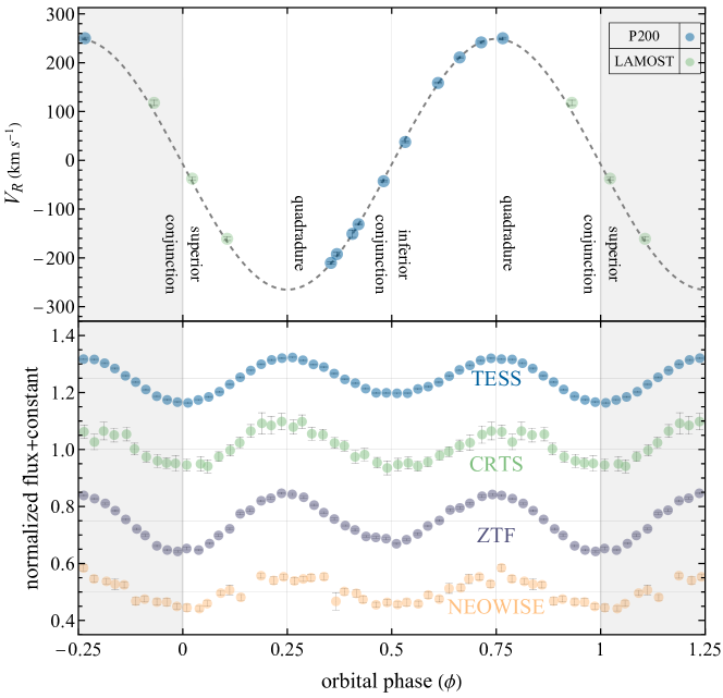
Figure 1: The phase-folded RV curve and the multi-band light curves for J1123. Upper panel: the RV curve. The green and blue points represent the exposures of LAMOST and P200, respectively. Lower panel: the phase-folded and smoothed light curves from TESS (blue), CRTS (green), ZTF r-band (purple), and NEOWISE W1-band (orange). All data are phase-folded with the ephemeris given in Equation (1), and smoothed by grouping the data into 40 equally spaced phase bins. The average within each bin is adopted. Data points are styled semi-transparent so the error bars (representing the $1$-sigma uncertainties) can be seen (zoom in to find black fences representing the error bars inside). The superior conjunction ($\phi$ $=$ 0 or 1), inferior conjunction ($\phi$ $=$ 0.5), and quadrature phases ($\phi$ $=$ 0.25 and 0.75) of the M dwarf are labeled and indicated by vertical grey lines. Horizontal grey lines in the lower panel indicate the mean of the normalized and vertically shifted light curve for each band. Points in shallow grey regions are duplicated ones for clarity. The RV curve and the light curves demonstrate the periodic Doppler shifts and ellipsoidal modulation effects caused by J1123’s invisible companion’s strong gravitational pull and tidal force.

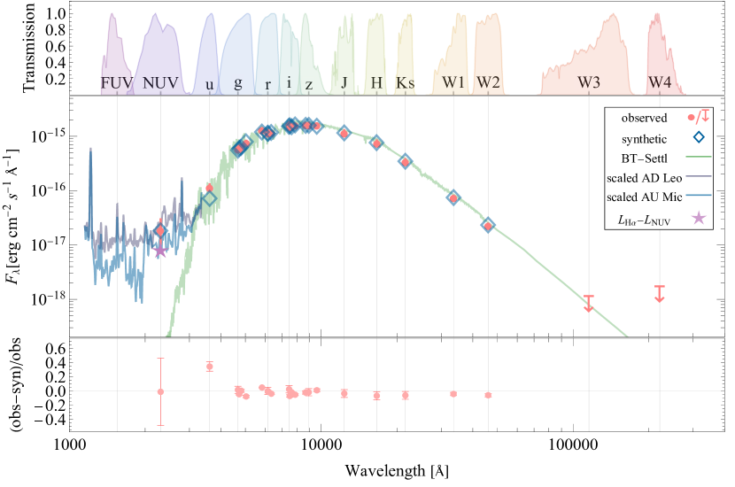
Figure 2: The broadband SED of J1123. Pink points are the observed flux from the GALEX NUV band, SDSS $ugriz$ bands, ZTF $gri$ bands, Gaia EDR3 BP-, RP- and G-bands, PanSTARRS $grizy$, 2MASS J H Ks bands, and AllWISE W1-W4 bands (bands for PanSTARRS, ZTF, and Gaia are not labeled to avoid overcrowding). Error bars represent the $1$-sigma uncertainties and downward arrows indicate upper limits for W3 and W4 bands. The green curve is the best-fit BT-Settl model spectrum for the M dwarf and blue hollow diamonds are the synthetic photometry by integrating the model SED over the transmission curve of each filter. Transmission curves for the filters of GALEX, SDSS, 2MASS, and WISE are displayed on the top panel and normalised at the maximum. To demonstrate that the observed UV excess is fully consistent with being produced by the chromospheric activities of the visible M dwarf, we scale on top of the SED the average UV spectrum of AD Leo (purple line), and of AU Mic (blue line). The mean synthetic NUV flux of these two M stars well matches the observation. Showing in the lower panel are the relative fit residuals, which is defined as (observed $-$ synthetic) $/$ observed. A predicted NUV flux for a sample of similar active M dwarfs[20] is also shown by the purple star (see text for the estimation by an empirical $L_{\mathrm{H\alpha}}$-$L_{\mathrm{NUV}}$ relation[20]).

Figure 3: The mass of the visible star ($M_{1}$) versus that of the hidden compact object ($M_{2}$). The violin width indicates the probability density distribution of $M_{2}$, which is obtained by fitting the ellipsoidal light-curve model to the TESS observations and RV variations for fixed $M_{1}$ and $R_{1}$. The four black short lines demonstrate the $1$-sigma and $2$-sigma ranges. The four solid blue curves correspond to the constraints from the mass function (Equation 2) for $\sin i$ $=$ 1, 0.95, 0.9, and 0.85, respectively; the blue-shaded regions represent the $1\sigma$ uncertainties. The grey-shaded regions illustrate the $1$-sigma uncertainties of $M_{1}$.

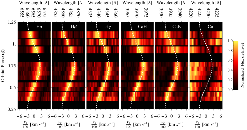
Figure 4: Phase-stacked Balmer (H$\alpha$ – H$\gamma$) emission lines, and Ca II H&K emission lines. The white dashed curve threading through the centers of each line represent the best-fit RV curve from fitting the photospheric absorption lines of the M dwarf (i.e., using CCF technique with all emission lines and telluric absorption lines masked). For comparison, the variation of the Ca I 4228Å absorption line is shown in the rightmost panel. It is evident that the emission lines are co-moving with the M dwarf, which suggests that they originate from the chromosphere of the M dwarf. Notes (a): two P200 exposures taken on June 2020 are not plotted to avoid overlapping; (b): the exposure time is 30 mins for LAMOST and 20 mins for P200.

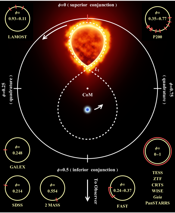
Figure 5: The viewing wheel of J1123 that summarises our best understanding of the system. J1123’s only visible component, an early-type M dwarf is gravitationally pulled by its invisible companion, a candidate NS (blue object). Two components are in orbiting with each other with an orbital period of $\sim$6.6 hours. An artistic impression of J1123’s active chromosphere is depicted (bright glowing region above the surface of the star), which induces substantial UV emissions as well as the emission lines. No signature of Roche lobe (white dashed line) overflow between two components suggests that the system is a non-accreting binary. Showing in corners, small yellow circles are copies of the orbit, and red marks denote the positions (phases) of the M star at which a specific observation was conducted.

References

The LAMOST low-resolution spectra can be queried at https://nadc.china-vo.org/data/data/sedr5/f?&locale=en. Raw TESS data are available from the MAST portal: https://archive.stsci.edu/missions-and-data/tess. The data can also be obtained from the corresponding author upon reasonable request.

The Lomb-Scargle module is publicly available on https://github.com/TuanYi/LombScargle. Reasonable requests for other materials and codes should be addressed to Wei-Min Gu (guwm@xmu.edu.cn).

We thank anonymous referees for providing numerous constructive suggestions that improved the quality of this paper. We thank Ya-Juan Lei, Daniel Price, Alexander Heger, Cui-Ying Song, Di Li, Xiao-Dian Chen, Wei-Kai Zong, Xiang-Gao Wang, Qiao-Ya Wu, Jun-Hui Liu, Xiao-Dan Fu, Yuan-Pei Yang, Xiao-Wei Liu, Yi-Han Song, and Tom Marsh for beneficial discussions. W.M.G. acknowledges support from the National Key R&D Program of China under grant 2021YFA1600401, and the National Natural Science Foundation of China (NSFC) under grants 11925301 and 12033006. M.Y.S. acknowledges support from NSFC under grant 11973002. J.F.L. acknowledges support from NSFC under grants 11988101 and 11933004. Z.X.Z. acknowledges support from NSFC under grant 12103041. J.F.Wang acknowledges support from NSFC under grant U1831205. J.F.Wu acknowledges support from NSFC under grant U1938105. X.D.L. acknowledges support from NSFC under grants 12041301 and 12121003. P.W. acknowledges support from NSFC under grant U2031117, the Youth Innovation Promotion Association CAS (id. 2021055), CAS Project for Young Scientists in Basic Research (grant YSBR-006) and the Cultivation Project for FAST Scientific Payoff and Research Achievement of CAMS-CAS. J.R.S. acknowledges support from NSFC under grant 12090044. J.Z. acknowledges support from NSFC under grant 11933008. H.J.M. acknowledges support from NSFC under grant 12103047. T.Y. acknowledges support from the China Postdoctoral Science Foundation under grant 2021M702742. Guoshoujing Telescope (the Large Sky Area Multi-Object Fiber Spectroscopic Telescope LAMOST) is a National Major Scientific Project built by the Chinese Academy of Sciences. Funding for the project has been provided by the National Development and Reform Commission. LAMOST is operated and managed by the National Astronomical Observatories, Chinese Academy of Sciences. This research uses data obtained through the Telescope Access Program (TAP), which has been funded by the TAP member institutes. This work made use of the data from FAST (Five-hundred-meter Aperture Spherical radio Telescope). FAST is a Chinese national mega-science facility, operated by National Astronomical Observatories, Chinese Academy of Sciences. Funding for the TESS mission is provided by NASA’s Science Mission directorate. This research made use of Lightkurve, a Python package for Kepler and TESS data analysis (Lightkurve Collaboration, 2018[7]). Based on observations obtained with the Samuel Oschin 48-inch Telescope at the Palomar Observatory as part of the Zwicky Transient Facility project. ZTF is supported by the National Science Foundation under Grant No. AST-1440341 and a collaboration including Caltech, IPAC, the Weizmann Institute for Science, the Oskar Klein Center at Stockholm University, the University of Maryland, the University of Washington, Deutsches Elektronen-Synchrotron and Humboldt University, Los Alamos National Laboratories, the TANGO Consortium of Taiwan, the University of Wisconsin at Milwaukee, and Lawrence Berkeley National Laboratories. Operations are conducted by COO, IPAC, and UW.

T.Y., W.M.G., and J.F.L. led the project. W.M.G. proposed the follow-up optical observations and coordinated the spectroscopic and photometric data reduction and analysis, with significant inputs from T.Y., M.Y.S., Z.X.Z., S.W., Y.B., and L.L.Z.. Z.R.B. and H.T.Z. contributed to the early discovery of J1123. W.M.G., J.F.Wang, and J.F.Wu contributed to their expertise of the P200 proposals and observations. Y.B. and Z.X.Z. contributed to the P200 data reduction and analyses. T.Y., Q.Z.Y., and W.M.G. proposed the follow-up radio observations. P.W. contributed to the expertise of FAST’s data reduction and analyses. Z.X.Z. and M.Y.S. solved the orbital solution using PHOEBE; S.W. and J.Z. validated the orbital solution independently. T.Y., W.M.G., M.Y.S., J.F.L., and P.W. presented the physical interpretation of the data and wrote the manuscript. All authors reviewed and contributed to the manuscript.

The authors declare no competing interests.

Readers are welcome to comment on the online version of the paper. Correspondence and requests for materials should be addressed to W.M.G. (email: guwm@xmu.edu.cn), M.Y.S. (email: msun88@xmu.edu.cn), or J.F.L. (email: jfliu@nao.cas.cn).

2.1 Observations and their reduction

I. Spectroscopy

Three low-resolution spectra (Supplementary Figure 1) were adopted from the first data-release of LAMOST low-resolution single epoch spectra[1]. Follow-up spectroscopy was obtained with DBSP mounted on the P200. The first observation (eight exposures; 20 minutes for each) was taken during a clear night on March 14, 2019, with an average seeing $\sim$ 2 arcsec. The DBSP covered a wavelength range of 3800 – 5400 Å with a resolving power $R$ $=$ 3400 for blue arm and 6000 – 7600 Å with $R$ $=$ 4900 for red arm (Supplementary Figure 2). We took HeNeAr and FeAr lamps for the wavelength calibration at the blue and red arms, respectively. Raw spectroscopic data was reduced by using the IRAF (Image Reduction and Analysis Facility). Standard IRAF procedures of bias subtraction, flat correction, cosmic-rays removal, 1D-spectrum extraction, wavelength calibration, and flux calibration were conducted. Wavelength calibration was performed by calibrating the HeNeAr and FeAr lamps to the corresponding spectral atlas provided by the Spectral Atlas Center. After the reduction, a few cosmic rays (sharp spikes typically occupy only a few pixels) remained uncleaned, thus we removed them manually. The second (remote) observation was taken on June 24, 2020 (two exposures), with similar details described above. Supplementary Table 2 is a complete observation log for spectroscopic observations.

II. Photometry

J1123 was classified by the Catalina Real-time Transient Survey (CRTS)[2] as a WUMa-type eclipsing binary, but it was later noted to be an ellipsoidal variable[3]. We collect multi-band light curves from: the CRTS, the Zwicky Transient Facility (ZTF)[4], the asteroid-hunting mission of the Wide-field Infrared Survey Explorer (NEOWISE)[5], and the Transiting Exoplanet Survey Satellite (TESS)[6].

J1123 was observed in sector 22 of TESS, with a monitoring time-span of roughly one month. The photometry of TESS was reduced by using the Lightkurve package[7]. We used the create_threshold_mask method to create single aperture and define background pixels. We tried different TESS cutout sizes, aperture shapes, and background sizes to perform background subtraction and light curve extraction, all reported well-consistent results. The simple background median subtraction method and also the PLD (pixel level de-correlation) method was used to extract the light curve.

2.2 The orbital period and ephemeris

We derived the orbital ephemeris (Equation (1)) by using the data of CRTS[2]. The period was searched by using the Lomb-Scargle periodogram[8, 9], with the generalized algorithm[10] and a fast implementation method[11]. By following VanderPlas’s prescription[12], we set the frequency grid to be uniformly spaced for the periodogram with an oversampling factor of ten; the lowest frequency is set to the reciprocal of the observation time-span $T_{\rm span}$, while the highest frequency is chosen as 500 times the average Nyquist frequency (i.e., Nyquist factor $=$ 500). The Lomb-Scargle powers report a significant period component $P_{\rm peak}$ $=$ 0.13691772 days (Supplementary Figure 3; upper panel). The true orbital period is thus twice the $P_{\rm peak}$ as the ellipsoidal light curve has two peaks and valleys, namely, $P_{\rm orb}$ $=$ 2$P_{\rm peak}$ $=$ 0.27383544(18) days. The uncertainty of $P_{\rm orb}$ (indicated by the last two digits inside the parenthesis) was derived by finding periods for a collection of bootstrap-resampled light curves. Periods for light curves of ZTF, NEOWISE, and TESS were searched by using the same technique with similar details, except for that the Nyquist factor for TESS was set to be one because of its 30-minutes observation cadence. Lomb-Scargle powers reported consistent results for all surveys (Supplementary Figure 3).

To find the M star’s superior conjunction, we folded the CRTS light curve with $P_{\rm orb}$ and a guessed reference HJD, denoted as HJD_guess. HJD_guess was taken to be the HJD of the point with the largest $V_{\rm mag}$ (smallest flux). Then the phase-folded light curve was fitted by a three-order Fourier series. The corresponding phase $\phi_{\rm min}$ at the best-fit’s minimum ($V_{\rm mag}$ maximum) was found, which is supposed to coincide with the superior conjunction ($\phi$ $=$ 0) of the M dwarf. The offset between the $\phi_{\rm min}$ and $\phi$ $=$ 0 helped us to update (correct) the HJD_guess and hence to derive the reference HJD at superior conjunction as $T_{0}$ $=$ 2 453 734.909 32 (31) HJD.

2.3 The radial velocities fitting method

To measure the RVs with respect to the Heliocentric rest-frame, we first use the baryvel function provided by PyAstronomy’s pyasl package to obtain the Heliocentric corrections for the mid-time of exposures and the RVs. All spectra are then shifted by the corresponding Heliocentric RV correction (Supplementary Table 2; column 10). As mentioned, chromospheric emission lines are presented in all of J1123’s spectra. We mask these emission lines as well as strong telluric absorption lines in 6860Å – 6950Å to measure the RV.

We use the PyHammer package[17] which implements the cross-correlation technique to measure the RVs with a library of observational spectra collected from the SDSS BOSS survey. The best-fitted template has a spectral type $=$ M1 and a metallicity $Z$ $=$ 0. Supplementary Figure 2 shows the template fitting of the last exposure taken by DBSP on Mar 14, 2019. The bootstrap re-sampling method is used to measure the values and uncertainties for RVs. For each spectrum, 3000 bootstrap re-samples are generated and fed to the PyHammer. The 50%, 16%, and 84% percentiles of the result RVs are read as the normial value, the lower error bar, and the upper error bar, respectively. We also fit the first three Balmer lines H$\alpha$ – H$\gamma$ to obtain their RV curves. The Gaussian function is used to fit the lines on the continuum-normalised spectrum.

Supplementary Table 2 shows the measured RVs; Supplementary Figure 4 shows comparisons for the RV curves of the first three Balmer lines (H$\alpha$, H$\beta$, and H$\gamma$) with the RV curve measured using only the absorption lines of the M star (i.e., all emission lines masked). Note that all reported RVs are measured in the Heliocentric rest-frame.

2.4 The spectral energy distribution fitting method

We construct the broadband SED of J1123 using archival photometric measurements from GALEX[13] (GALEX reported a detection of NUV $=$ 22.73 $\pm$ 0.52 mag but no detection of FUV), SDSS[14] ($ugriz$ bands), Gaia EDR3[18] (BP, RP, and G bands), ZTF[4] ($gri$ bands), PanSTARRS[15] ($grizy$ bands), 2MASS[16] (J, H, and Ks bands), and AllWISE[17, 18] (W1–W4 bands). The distance is $D=318\pm 4$ pc since the parallax $\bar{\omega}$ $=$ 3.147 $\pm$ 0.038 mas (Gaia EDR3[18]), and the extinction $E(B-V)$ $=$ 0.019 $\pm$ 0.001 is referred to the PanSTARRS 3D dust extinction map[19]. Supplementary Table 3 shows the collected archival photometric data.

We do not use GALEX NUV and SDSS u-band data when fitting SED, since one does not have prior knowledge of the origin of these emissions. To measure the average temperature and the average radius of the M dwarf, the mean flux is required in the SED fitting[20]. Some of the surveys have sparse observations; for instance, 2MASS and SDSS both have observed J1123 only once. To account for the fact that these measurements are phase-dependent, we accommodate additional systematic flux uncertainties = $F_{\lambda}\times 5\%/\sqrt{N}$ for all bands, where 5% is the standard deviation of the TESS light curve variations and $N$ is the number of observations for each band. We also add additional 1% uncertainties for all the ground-based surveys, i.e., SDSS, PanSTARRS, ZTF, and 2MASS, to account for the typical photometric zero-point uncertainties.

We used the Cardelli extinction curve[21] and the R_V $=$ 3.1 reddening law[22] to correct the reddening. A grid of synthetic photometry is constructed by integrating the transmission curves of the filters over the BT-settl[23] synthetic model SED. All synthetic SEDs and transmission curves were adopted from VOSA (virtual observatory SED analyzer)[24]. The grid span of effective temperature is 3000 – 5000 K, with a step size of 100 K; and the span of surface gravity is 4.0 – 5.5 dex, with a step size of 0.5 dex. A Solar metallic abundance ($Z$ $=$ 0) is fixed by referring to the metallicity of the best-fitted PyHammer spectral template. A linear interpolation is used (based on values at grid nodes) to approximate the synthetic photometry at arbitrary points inside the pre-calculated grid.

Prepared with the interpolated synthetic photometry grid, we use a MCMC sampler with the Metropolis-Hastings algorithm to fit the observed SED. We define the likelihood function $\mathcal{L}$ as

$$\ln\mathcal{L}(\mathcal{D}|\mathcal{M}(R_{1},D,T_{\mathrm{eff,~{}1}},\log{g}))=-\frac{1}{2}\sum_{\mathrm{band}}\left(\frac{F_{\rm obs,band}-(\frac{R_{1}}{D})^{2}\times F_{\rm syn,band}(T_{\mathrm{eff,~{}1}},\log{g})}{\sigma_{F}}\right)^{2}\ ,$$ (3)

where $\mathcal{D}$ is the observed SED data set, $\mathcal{M}$ is the model SED given the parameters: $R_{1}$ (stellar radius), $D$ (distance), $T_{\mathrm{eff,~{}1}}$ (effective temperature), and $\log{g}$ (surface gravity). $F_{\rm obs,band}$ is the observed flux at a specific band, $(R_{1}/D)^{2}$ is the dilution factor, $F_{\rm syn,band}(T_{\mathrm{eff,~{}1}},\log{g})$ is the synthetic flux at a specific band, and $\sigma_{F}$ is the flux uncertainties. Thus the MCMC sampler updates the prior distributions of our target parameters according to the Bayes Theorem:

$$\mathcal{\pi}(\mathcal{M}(R_{1},D,T_{\mathrm{eff,~{}1}},\log{g})|\mathcal{D})\propto\mathcal{L}(\mathcal{D}|\mathcal{M}(R_{1},D,T_{\mathrm{eff,~{}1}},\log{g}))\times\prod_{x\in X}\mathcal{P}(x)\ ,$$ (4)

where $\mathcal{\pi}$ is the posterior distributions of the parameters given the data; $\mathcal{P}(x)$ is the prior distribution of a parameter $x$ in the target parameter set $X$ $=$ ($T_{\mathrm{eff,~{}1}}$, $R_{1}$, $D$, $\log{g}$). The sampler uses the logarithm of the posterior, i.e., $\ln(\mathcal{\pi})$ in real implementation. The chain took 200 000 steps with the first 100 000 points dropped as the burn-in. The prior distributions and posterior distributions of these parameters are listed in Supplementary Table 1. The marginal and joined posterior distributions are presented in Supplementary Figure 5.

2.5 The mass of the M dwarf

Here we describe details of the isochrones fitting. The BT-Settl isochrones are again retrieved from the VOSA; only isochrones with zero metallicity ($Z$ $=$ 0) are used. These isochrones cover complete stellar ages, ranging from 0.001 Gyr up to 12 Gyr. However, the mass grid is not fine enough, e.g., only $M$ $=$ 0.45, 0.5, 0.57, 0.60, 0.62, 0.70, and 0.75 $M_{\odot}$ is provided for early-type M dwarfs or late-type K dwarfs. Thus a linear interpolation is implemented to populate the mass grid in 0.45-0.75 $M_{\odot}$ mass range, with a finer step size of 0.01 $M_{\odot}$ bins.

By assuming the distribution is log-normal, the likelihood for observing the M dwarf’s effective temperature $T_{\mathrm{eff,1}}$ and bolometric luminosity $L_{\mathrm{bol,1}}$, given a stellar mass $M_{*}$ can be calculated by:

$$\mathcal{L}(T_{\mathrm{eff,~{}1}},L_{\mathrm{bol,~{}1}}|M_{*})=\sum\frac{1}{2\pi\sigma_{\log{T}}\sigma_{\log{L}}}\exp\left(-\frac{(\log T_{\mathrm{eff,~{}1}}-\log T_{{\rm eff},~{}M_{*}})^{2}}{2\sigma_{\log{T}}^{2}}-\frac{(\log L_{\mathrm{bol,~{}1}}-\log L_{{\rm bol},~{}M_{*}})^{2}}{2\sigma_{\log{L}}^{2}}\right)\ ,$$ (5)

where the summation sign denotes the summation over all isochrones. $T_{{\rm eff},~{}M_{*}}$ and $L_{{\rm bol},~{}M_{*}}$ are the effective temperature and the bolometric luminosity given the stellar mass $M_{*}$ in an isochrone, and $\sigma_{T}$ and $\sigma_{L}$ are the uncertainties of $\log T_{\mathrm{eff,~{}1}}$ and $\log L_{\mathrm{bol,~{}1}}$, respectively. We adopted a Kroupa initial mass function[25] as the prior of the stellar mass, denoted as IMF. Thus according to the Bayes theorem, the probability distribution (posterior) of stellar mass $M_{*}$ given the observed $T_{\mathrm{eff,~{}1}}$ and $L_{\mathrm{bol,~{}1}}$ is: $\pi(M_{*}|T_{\mathrm{eff,~{}1}},L_{\mathrm{bol,~{}1}})$ $\propto$ $\mathcal{L}(T_{\mathrm{eff,~{}1}},L_{\mathrm{bol,~{}1}}|M_{*})$ $\times$ IMF. The result posterior is obtained by fitting a Gaussian on the interpolated mass grid (Supplementary Figure 6; right panels).

We obtain a stellar mass $M_{1}$ $=$ 0.60 $\pm$ 0.02 $M_{\odot}$ of the M dwarf by fitting the model BT-Settl isochrones. Note that this approach could have uncertainty when dealing with a tidally locked star in close binaries. According to previous studies[26], stellar dynamo and magnetism[27] can inflate the radii of low-mass stars ($<$0.8 M_⊙). For tidally locked stars in close binaries, rapid rotation enhances the magnetic field[28] and induces more spots groups on the star’s surface. Thus the star turns to be cooler than its single main-sequence (MS) siblings of the same type. The consequence is that the star is ‘bloated’, the radius is inflated to balance the total output energy generated within the stellar interior. Components in short-period ($\lesssim$1 day) binary systems can have radii being inflated by $\sim$4.8% $\pm$ 1.0%[29] with respect to single low-mass MS stars. Thus we deflate 5% of the SED derived radius. Assuming that the bolometric luminosity is conserved during the tidal distortion process, this correction results in $\sim$2.6% increase of the effective temperature (pink point in Supplementary Figure 6; left panel). The fitting of isochrone thus results in a slightly larger mass $M_{1}$ $=$ 0.61 $\pm$ 0.02 $M_{\odot}$.

As an independent check, we use an empirical mass-luminosity relation (MLR) for the MS M dwarfs (Equation (11) in Benedict et al. (2016)[30]) and the 2MASS Ks-band absolute Magnitude ($=$ $K_{\mathrm{mag}}$ $+$ 5 $-$ 5$\log D$ $-$ $A_{\mathrm{K}}$ $=$ 5.18 $\pm$ 0.04, where $K_{\mathrm{mag}}$ $=$ 12.699 $\pm$ 0.023 and $A_{\mathrm{K}}$ $=$ 0.0068 $\pm$ 0.0004) to estimate the mass of the visible M dwarf. We obtain $M_{1}=0.62\pm 0.02M_{\odot}$, which is similar to the result from the model isochrone fitting. We adopt the isochrone mass $M_{1}$ $=$ 0.61 $\pm$ 0.02 $M_{\odot}$, as the mass of the M dwarf.

2.6 The orbital solution by the PHOEBE software

To obtain the orbital inclination $i$, the mass ratio $q\,(\equiv M_{2}/M_{1})$, and thus the compact object’s mass $M_{2}$, we fit simultaneously the RV curve and the TESS light curve using PHOEBE 2.3[31, 32, 33]. The orbital period ($P_{\rm orb}$ $=$ 0.27383544 days) is fixed. For the compact object (secondary), we set distortion_method $=$ none such that it is treated like an object without flux contributions and eclipse effects. For the M dwarf (primary), the effective temperature ($T_{\mathrm{eff,~{}1}}$ $=$ 3769 K) is fixed. We obtain the limb-darkening($u$) coefficient and the gravity-darkening($\tau$) coefficient in TESS band by using Claret 2017[34]’s limb-darkening and gravity-darkening tables. The results are: $\tau$ $=$ 0.32 for gravity-darkening, and ($e$, $f$) $=$ (0.684, 0.389) for a logarithmic limb-darkening law (refer to Equation (4) in Claret 2017[34]). The PHOENIX atmospheric model is used.

The first model (hereafter model A) we considered is the canonical ellipsoidal modulations[35, 16, 36, 37] with $M_{1}=0.61\ M_{\odot}$ and $R_{1}=0.63\ R_{\odot}$. Given $i$ and $M_{2}$, the logarithmic likelihood of the observed TESS light curve is

$$\ln\mathcal{L}(\mathrm{TESS\ LC}|i,M_{2},\mathrm{model\ A})=-\frac{1}{2}\sum\left[\frac{(f_{\mathrm{m}}-f_{\mathrm{obs}})^{2}}{\sigma_{\mathrm{tot}}^{2}}+\ln{(2\pi\sigma_{\mathrm{tot}}^{2})}\right]\\ ,$$ (6)

where $f_{\mathrm{m}}$ and $f_{\mathrm{obs}}$ represent the model and observed TESS fluxes, respectively; $\sigma_{\mathrm{tot}}^{2}=\sigma_{\mathrm{obs}}^{2}+\sigma_{\mathrm{sys}}^{2}$ and the latter two represent the uncertainties of the observed TESS fluxes and the systematic uncertainties (which accounts for additional factors, e.g., starspot, that were not included in the model). The ellipsoidal modulation fluxes are calculated via PHOEBE. Similarly, we can calculate the logarithmic likelihood of the observed RV variations for every $i$ and $M_{2}$, i.e.,

$$\ln\mathcal{L}(\mathrm{RV_{obs}}|i,M_{2},\mathrm{model\ A})=-\frac{1}{2}\sum\left[\frac{(v_{\mathrm{m}}-v_{\mathrm{obs}})^{2}}{\sigma_{v}^{2}}+\ln{(2\pi\sigma_{v}^{2})}\right]\\ ,$$ (7)

where $v_{\mathrm{m}}$, $v_{\mathrm{obs}}$ and $\sigma_{v}$ represent the model RV, the observed RV and its uncertainty. The prior distributions for the model parameters are assumed to be uniform. The Markov Chain Monte Carlo Ensemble sampler code emcee[38] is used to sample the posterior probability density, i.e., the product of the likelihood (whose logarithmic value is the summation of Equations 6 and 7) and the uniform prior probability. We implement 50 parallel chains, each with 10 000 steps. The results are $i=73^{+1.8}_{-1.5}$ degree and $M_{2}=1.24^{+0.03}_{-0.03}\ M_{\odot}$. The fitting result is presented in Supplementary Figure 7. It is clear that the residuals between the model and the observed fluxes show periodic variations. The Akaike Information Criterion (AIC) and Bayesian Information Criterion (BIC) for this fit are $-348$ and $-337$, respectively.

Motivated by the periodic variations in the residuals, we consider the following two models: a model with ellipsoidal modulations and a hotspot (hereafter model B); a model with ellipsoidal modulations and a coldspot (hereafter model C). We find that models B and C eliminate the periodic residuals (see Supplementary Figure 7). The AICs and BICs for the two models are smaller than those of model A by a factor of $60$. Statistically speaking, models B and C are preferred over model A. To fully propagate the uncertainties of $M_{1}$ and $R_{1}$ to our estimation of $i$ and $M_{2}$, we now also let $M_{1}$ and $R_{1}$ in models B and C to vary; we set Gaussian priors for $M_{1}$ and $R_{1}$ according to the isochrone mass and the SED radius, i.e., $\mathcal{N}(0.61M_{\odot},0.02M_{\odot})$ for $M_{1}$ and $\mathcal{N}(0.63R_{\odot},0.01R_{\odot})$ for $R_{1}$. For model B, the results are $i=71_{-7.2}^{+10}$ degree and $M_{2}=1.26_{-0.09}^{+0.13}\ M_{\odot}$; for model C, the results are $i=64_{-4.9}^{+6.3}$ degree and $M_{2}=1.4_{-0.11}^{+0.12}\ M_{\odot}$. Models B and C cannot be distinguished since their AICs and BICs are similar. We stress that the three inferred $M_{2}$ are statistically consistent (within $1.5$-sigma uncertainties).

2.7 Could a distant third body exist in J1123?

Triple systems are not rare in the Galaxy. Could a distant third body (i.e., the tertiary) exist in J1123? To address the issue, we use two techniques that are popular for characterizing spectroscopic binaries or triples[39, 40, 41, 42, 43]: the cross-correlation function (CCF)[44] and the broadening function (BF).[45, 46] We create a theoretical template having the same stellar parameters as J1123, by interpolating the theoretical BT-settl models[23] for low-mass stars. Using the template, the CCFs and the BFs for P200 spectra are calculated in the velocity range $(-500\mathrm{\,km\,s^{-1}}$, $500\mathrm{\,km\,s^{-1}})$ and for three wavelength ranges: 4360 – 4800 Å, 5190 – 5360 Å, and 6050 – 6280 Å (as they are free of emission lines, telluric absorption, and provide fine matches to the theoretical template). The final result is obtained by averaging the results of these three wavelength ranges (Supplementary Figure 8).

For comparison, we create mock data using the same BT-Settl template, to simulate the spectrum for a triple system scenario with a distant third star plus an inner binary (M star + compact object). Only the wavelength range 6000 – 7000 Å is used for simplicity. For the M star, we artificially broaden the spectrum with a rotational broadening kernel[47] corresponding to $v\sin{i}=\omega R_{1}\sin{i}=(2\pi/P_{\rm orb})R_{1}\sin{i}\simeq 111\mathrm{\,km\,s^{-1}}$. The spectrum is then shifted to the corresponding RV at a specific phase. For the third star, we assume that it is a slow rotating one; a rotational broadening kernel with $v\sin{i}=10\mathrm{\,km\,s^{-1}}$ is applied. We also assume that the third star’s RV is sufficiently small, i.e., $V_{\rm R}\simeq\gamma=-8\mathrm{\,km\,s^{-1}}$ in the case of a very wide outer orbital separation or the case of a nearly face-on outer orbit. The luminosity of the third star is assumed to be $0.5$, $0.2$, or $0.1$ times that of the M dwarf. The two mock spectra are superimposed, degraded to a resolution $R=4900$ similar to our P200 spectra, and Gaussian noise is added according to the signal-to-noise ratio of the corresponding real spectrum. The CCFs and the BFs are then calculated by using the mock spectra and the template from which these mock spectra are generated.

A prominent secondary peak is expected in the CCFs and BFs of the mock data if the distant third object is contributing a non-negligible ($\gtrsim 10\%$) fraction of flux (lower sub-panels of Supplementary Figure 8). On the contrary, both CCFs and BFs for J1123 observations show single-peaked shapes, in well agreement with a single-lined spectroscopic binary. The comparison between the CCFs and BFs of real observations and those of our mock data suggests that the possible tertiary should be one order of magnitude fainter than the visible M dwarf.

In addition, high precision Gaia astrometry measured an astrometric excess noise $\epsilon=0\pm 0$ mas and a renormalized unit weight error[48] ruwe $=$ 1.008. Instead, wide binaries or triple systems in the Solar neighbourhood tend to have a significantly larger excess noise[49] or a ruwe significantly deviates from one[50]. Hence, the two Gaia astrometric parameters suggest that J1123’s astrometric solution is inconsistent with the triple system scenario.

2.8 The H$\alpha$ luminosity, UV excess, and the chromospheric activity

To obtain the H$\alpha$ luminosity, we scale the target spectra to match the model SED in the first place. The model SED at a wavelength range 6564.61 $\pm$ 30 Å around the H$\alpha$ is subtracted and the total H$\alpha$ flux $F_{\mathrm{H\alpha}}$ can then be summed up. The H$\alpha$ luminosity $L_{\mathrm{H\alpha}}$ $=$ $F_{\mathrm{H\alpha}}\times 4\pi R_{1}^{2}\times(R_{1}/D)^{-2}$, i.e., $\simeq$ $2\times$$10^{28}$ erg s^-1, or equivalently, $\simeq$ 5.3$\times$$10^{-6}$$L_{\odot}$ (average over all 13 spectra).

J1123 was recognized to be an UV emitting star by Bai et al. (2018)[51]. GALEX’s All-sky Imaging Survey (AIS) has observed J1123 on Feb 14, 2007. Both NUV and FUV filters took 136 seconds’ exposure simultaneously, but only NUV has reported detection of NUV $=$ 22.73 $\pm$ 0.52 mag (AB magnitude system). GALEX’s observation was taken at the orbital phase $\phi$ $=$ 0.248, near the quadrature-phase when two components were side by side. Thus the compact object was not obscured by the M dwarf but being fully exposed to the observer.

The extinction corrected GALEX NUV flux $F_{\mathrm{NUV}}$ $=$ (1.9 $\pm$ 0.9) $\times$ 10^-17 erg s^-1 cm^-2 Å^-1, thus the NUV luminosity $L_{\mathrm{NUV}}$ $\approx$ $F_{\mathrm{NUV}}$$\times$$\mathrm{W_{eff}}$$\times$$(R_{1}/D)^{-2}$$\times$4$\pi$$R_{1}^{2}$ $=$ (1.8$\pm$0.8)$\times$10²⁹erg s^-1, where $\mathrm{W_{eff}}$ $=$ 768.31Å is the effective width of NUV. We calculate the excess of UV luminosity by subtracting the base UV emission from the photosphere. The latter is obtained by integrating the model SED in the NUV band, which yields $L_{\mathrm{base}}$ $\approx$ 1.0$\times$10²⁸ erg s^-1. Thus, the UV excess can be calculated as $R_{\mathrm{NUV}}$ $=$ ($L_{\mathrm{NUV}}-L_{\mathrm{base}}$) $/$ $L_{\mathrm{bol}}$ $=$ 0.00063 $\pm$ 0.00032 and $\log{R_{\mathrm{NUV}}}$ $=$ $-$3.20$\pm$0.22. The empirical $L_{\mathrm{H\alpha}}$ - $L_{\mathrm{NUV}}$ relation[20] predicts that $\log$($L_{\mathrm{NUV}}/L_{\mathrm{bol}}$) $=$ 0.67$\times$ $\log$($L_{\mathrm{H\alpha}}/L_{\mathrm{bol}}$) $-$ 0.85 $\approx$ $-$3.5 (or equivalently, 8.8 $\times$ 10^-18 erg s^-1 cm^-2 Å ^-1), provided that $\log$(${\overline{L}_{\mathrm{H\alpha}}}/L_{\mathrm{bol}}$) $\approx$ $-$4.

The UV spectra of AD Leo and AU Mic, two single M dwarfs, were retrieved from the Mikulski Archive for Space Telescopes (MAST). Both sources were observed by the IUE (International Ultraviolet Explorer)[52, 53] multiples times. For each source, we collect all the low dispersion spectra, take the average spectrum, and convolve the average by an 1 Å kernel to increase the signal-to-noise ratio. We scale the UV spectra according to (a similar method described by Rugheimer et al. (2015)[54] ):

$$F_{\mathrm{UV~{}J1123}}=F_{\mathrm{UV~{}AD/AU}}\times\left(\frac{T_{\mathrm{eff~{}J1123}}}{T_{\mathrm{eff~{}AD/AU}}}\right)^{4}\times\frac{\mathrm{log}(L_{\mathrm{H\alpha~{}J1123}}/L_{\mathrm{bol~{}J1123}})}{\mathrm{log}(L_{\mathrm{H\alpha~{}AD/AU}}/L_{\mathrm{bol~{}AD/AU}})}\times\left(\frac{R_{\mathrm{J1123}}}{R_{\mathrm{AD/AU}}}\times\frac{D_{\mathrm{AD/AU}}}{D_{\mathrm{J1123}}}\right)^{2}\ ,$$ (8)

where the subscript AD/AU stands for AD Leo or AU Mic. The adopted stellar parameters for two sources and references are listed in the Supplementary Table 4. The synthetic NUV flux from the chromosphere is then calculated by integrating the UV spectrum with GALEX NUV transmission curve. The mean NUV flux of two sources is adopted as the final estimated synthetic photometry.

2.9 FAST observation of J1123 and data reduction

The FAST observation of J1123 was conducted on September 7, 2021. The total integration time was 3000 seconds (the first two minutes and the last two minutes was for calibration signal injection time). The centre frequency was 1.25 GHz, spanning from 1.05 GHz to 1.45 GHz, including a 20-MHz band edge on each side. The average system temperature was 25 K. The recorded FAST data stream for pulsar observations is a time series of total power per frequency channel, stored in PSRFITS format (Hotan et al., 2004)[55] from a ROACH-2 based backend, which produces 8-bit sampled data over 4k frequency channels at 49 $\mu$s cadence. We searched for radio pulsations with either a dispersion signature or instrumental saturation in all FAST data collected during the observational campaign. Three types of data processing were performed: I) dedicated (half-blind) periodic pulse search, single pulse search and baseline saturation search.

I. Dedicated (half-blind) search:

Based on the Galactic electron density model NE2001[56] and YMW16[57], we estimate the distance $D$ $=$ 318 $\pm$ 4 pc corresponding with a DM of $\sim$ 3.2 pc cm^-3, and the line of sight maximal Galactic DM (max) $=$ 12 pc cm^-3. Due to model dependence and for the sake of robustness, we set the range of dispersion search as approximately zero to four times the estimated DM (max), namely, DM $=$ 0 – 50 pc cm^-3, which should cover all uncertainties. We used the output of PRESTO’s DDPlan.py package (Ransom et al., 2001[58]) to establish the de-dispersion strategy. The step size between subsequent trial DMs ($\Delta$DM = 0.1 pc cm^-3) was chosen such that over the entire band $t$($\Delta$DM) $=$ $t_{\rm channel}$. This ensures that the maximum extra smearing caused by any trial DM deviating from the source DM by $\Delta$DM is less than the intra-channel smearing. For each of the trial DMs, we searched for a periodical signal and the first and second order (jerk search; Andersen & Ransom, 2018 [59]) acceleration in the power spectrum based on the PRESTO pipeline (Wang et al. 2021)[60]. We checked all the pulsar candidates of signal-to-noise-ratio (SNR) $>$ 5 one by one and identified them as narrow-band radio frequency interferences (RFIs).

II. Single pulse search:

We used the above dedicated search scheme to de-disperse the data. Then we used 14 box-car width match filter grids distributed in logarithmic space from 0.1 ms to 30 ms. A zero-DM matched filter was applied to mitigate RFI in the blind search. All the possible candidate plots generated were then visually inspected. Most of the candidates were RFIs, and no pulsed radio emission with dispersive signature was detected with a SNR $>$ 5.

III. Saturation search:

We understand that if the radio flux is as high as kilojansky–megajansky, FAST would be saturated. We therefore also searched for saturation signals in the data. We looked for the epoch in which 50$\%$ of channels satisfy one of the following conditions: 1) the channel is saturated (255 value in 8-bit channels), 2) the channel is zero-valued, 3) the RMS of the bandpass is less than 2. We did not detect any saturation lasting $>$ 0.5 s, hence excluded any saturation associated during the observational campaign.

IV. Notes on the acceleration searches:

Since the orbital period (6.6 hr) is longer than about 8 times the observation duration (3000 sec), we carried out acceleration searches for the binary pulsar candidate using line acceleration ($Z_{\rm max}=$300) and jerk ($W_{\rm max}=$100) terms in the Fourier domain (PRESTO). This corresponds to a maximum drift of physical linear acceleration $Z_{\rm max}\cdot c\cdot P_{\rm spin}/N_{\rm harm}/T_{\rm obs}^{2}$, where c is the speed of light, $P_{\rm spin}$ is the spin period of the pulsar, and $T_{\rm obs}$ = 3000 s is the effective integration time. We note that all acceleration and jerk effects affect higher harmonics of a pulsar signal more than they do the fundamental ones. For a non-recycled NS, assuming the typical $P_{\rm spin}=$ 20 and 200 ms pulsar detected with up to eight harmonics ($N_{\rm harm}=8$, incoherently summarizing possible harmonics in fundamentals to increase the SNR), the maximum linear accelerations are $\sim$25 and $\sim$250 m s^-2, respectively. That is, the range of linear acceleration are ($-$25, 25) and ($-$250, 250) m s^-2. For the ‘jerk’ search, the constant jerk corresponds to a linearly varying acceleration: $W_{\rm max}\cdot c\cdot P_{\rm spin}/N_{\rm harm}/T_{\rm obs}^{3}$, hence the maximum jerk acceleration can be separately approximated as $\sim$0.003 and $\sim$0.03 m s^-3, i.e., the range of jerk acceleration are ($-$0.003, 0.003) and ($-$0.03, 0.03) m s^-3, assuming the same $P_{\rm spin}=$ 20 and 200 ms.

We note that the acceleration and the jerk searching effects highly depend on the orbital phase of the NS. For J1123, our FAST observation corresponds to the M star’s phases in between $\phi=$ 0.24 – 0.37, or equivalently, the NS’s phases in between $\phi=$ 0.74 – 0.87. Utilizing the well-measured RV curve of the M star, the inferred RV curve for the NS can be written as: $V_{\rm R,NS}=(K_{1}/q)\cdot\sin((2\pi/P_{\rm orb})t)+\gamma$, where $q=2.04\pm 0.04$ is the dynamically constrained mass ratio. We estimated the variation of the linear acceleration and the jerk of the NS using the first and the second derivative of the NS’s RV curve: $V^{\prime}_{\rm R,NS}=(K_{1}/q)\cdot(2\pi/P_{\rm orb})\cdot\cos((2\pi/P_{\rm orb})t)$ and $V^{\prime\prime}_{\rm R,NS}=-(K_{1}/q)\cdot(2\pi/P_{\rm orb})^{2}\cdot\sin((2\pi/P_{\rm orb})t)$, respectively. Thus the range of the linear acceleration and the jerk are (2.1$\pm$0.1, $-$22.9$\pm$0.4) m s^-2 and ($-$0.0089$\pm$0.0002, $-$0.0065$\pm$0.0002) m s^-3, respectively. Based on our estimation above, the parameter space for pulsar search is sufficient for the radio pulse search of this binary system.

2.10 The proper motion and the Galactic position of J1123

The proper motion of J1123 is[18] $\mu_{\alpha}=-20.604\pm 0.034\,\mathrm{mas\,yr}^{-1}$ in the R.A. direction and $\mu_{\delta}=-24.276\pm 0.036\,\mathrm{mas\,yr}^{-1}$ in the Dec. direction, thus the total proper motion is $\mathrm{pm}=31.841\pm 0.035\,\mathrm{mas\,yr}^{-1}$. Located at a distance $D=318\pm 4$ pc, the transverse velocity on the projected plane of the sky is $V_{T}\approx\mathrm{pm}\times D=48.0\pm 0.6\,\mathrm{km\,s}^{-1}$ and the space velocity is $V=\sqrt{V_{T}^{2}+V_{R}^{2}}=48.7\pm 0.7\,\mathrm{km\,s}^{-1}$.

The Galactic longitude and latitude of J1123 is $l=$ 171.85948 degree and $b=$ 67.58776 degree, respectively, placing it on a height $z\approx z_{\odot}+D\sin{b}$ $\simeq$ 319 pc above the Galactic plane (where $z_{\odot}$ $=$ 25 pc is the height of our Sun above the Galactic plane[61]). By using the pyasl package in PyAstronomy, we calculate J1123’s Galactic space velocity relative to the local standard rest as $(U,V,W)=(-1.4~{}{\rm km~{}s^{-1}},-33.5~{}{\rm km~{}s^{-1}},-3.8~{}{\rm km~{}s^{-1}})$. We use the method described by Bensby et al. 2003[62] to calculate the relative probability for the thick-disc-to-thin-disc membership, qualified as TD/D. We find that TD/D = 0.028, that is, J1123 most likely belongs to the thin disc.

2.11 Characterizing the possible massive, cold WD

As mentioned in the paper, the possibility that a massive cold WD resides in J1123 cannot be fully ruled out. Here, we constrain the temperature of of the possible WD. We adopt theoretical WD atmospheric models[63] plus the best-fit M dwarf’s SED to construct composite SEDs (Supplementary Figure 9). Four DA type WD models with a same surface gravity $\log{g}$ $=$ 9.0 but different effective temperatures ($T_{\mathrm{eff,WD}}$ $=$ 50 000 K, 20 000 K, 10 000 K, and 8000 K) are adopted. The WDs’ radius $R_{\rm WD}$ $\approx$ 0.0057 $R_{\odot}$ corresponds to the mass $M_{\mathrm{WD}}=$1.2$M_{\odot}$. The WD SEDs are scaled to J1123’s distance ($D=318$ pc) by multiplying the dilution factor $(R_{\rm WD}/D)^{2}$.

Supplementary Figure 9 compares the composite SED (purple curve) and its synthetic flux (hollow purple diamonds) with the observed P200 spectrum and photometric fluxes. WDs with $T_{\mathrm{eff,WD}}$ $=$ 50 000 K or 20 000 K are ruled out since models predict higher fluxes than the observations at the GALEX NUV band or SDSS u-band. A WD with $T_{\mathrm{eff,WD}}$ $\approx$ 10000K can account for the NUV flux. In the realistic case, since the SED contains a substantial amount of chromospheric UV emission, the possible WD is even colder, that is, $T_{\mathrm{eff,WD}}<$10 000K.

A recently discovered detached post-common-envelope binary (PCEB) SDSS J1140+1542[64] (J1140 for short) contains a similar massive cold WD with $M_{\mathrm{WD}}>1.22M_{\odot}$ and $T_{\mathrm{eff~{}WD}}=8900\pm 900$K. The companion of J1140 has a spectral type M2.5, a slightly cooler M dwarf with $T_{\mathrm{eff}}$$\sim$3400 K, and only half of J1123’s luminosity (i.e., $L_{\mathrm{bol~{}J1140}}$$\sim$0.035$L_{\odot}$) as reported by Gaia. Due to its relatively faint companion, the WD nature of J1140 was able to be revealed by the spectral decomposition method. In fact, a handful of magnetic WDs[65, 66] in detached PCEBs were found to be systematically much cooler ($T_{\mathrm{eff~{}WD}}\lesssim 10000$K), more massive, and close to Roche lobe filling than non-magnetic ones[64]. But again, these magnetic systems are lower in companion masses as their spectral types are typically later than M3.0. Therefore if the compact object in J1123 is a WD, the WD must be cold and massive, which can be hardly found by conventional (non-time-domain) WD surveys.

2.12 Investigating the irradiation effects

I. NS + irradiating M star case:

We simulate the TESS light curve for the case of a NS + M star binary with irradiation effects using PHOEBE (the left panels of Supplementary Figure 10). We use 100 sets of orbital parameters randomly drew from the distributions of the PHOEBE’s orbital solution to simulate the light curves.

We consider three irradiation luminosities, $L_{\mathrm{irr}}=$ $4.2\times 10^{32}\ \mathrm{erg\ s^{-1}}$, $6.4\times 10^{31}\ \mathrm{erg\ s^{-1}}$, and $1.6\times 10^{30}\ \mathrm{erg\ s^{-1}}$. It is evident that for $L_{\mathrm{irr}}\gtrsim 6.4\times 10^{31}\ \mathrm{erg\ s^{-1}}$, the resulting model light curve is inconsistent with the TESS observations (Supplementary Figure 10; left upper and middle panels). The nose of the M star (the side facing the inner Lagrange point) is heated up by the incident energy, partitioning the M star into a noticeable “day-side” (near $\phi=0.0$) and a “night-side” (near $\phi=0.5$ ). Hence, we conclude that $L_{\mathrm{irr}}\lesssim 6.4\times 10^{31}\ \mathrm{erg\ s^{-1}}$.

The energy source of the irradiation is probably powered by the pulsar wind of the NS. About $20\%$[67] of the pulsar wind power is reprocessed and heats up the M dwarf. Hence, according to the analyses above, the wind power of J1123 should be $L_{\mathrm{wind}}\lesssim 3.2\times 10^{32}\ \mathrm{erg\ s^{-1}}$. The possible pulsar wind in J1123 should be driven by the spin-down energy of the NS (rather than the accretion power since J1123 is a non-accreting system). Therefore, the spin-down power $L_{\mathrm{sd}}$ should also be less than $3.2\times 10^{32}\ \mathrm{erg\ s^{-1}}$. The spin-down rate of a NS is determined by $\dot{P}_{\rm spin}=(L_{\rm sd}P_{\rm spin}^{3})/(4\pi^{2}I_{\rm NS})$, where $I_{\rm NS}=(2/5)\cdot M_{\rm NS}R_{\rm NS}^{2}\simeq 1.4\times 10^{45}~{}\mathrm{g~{}cm^{2}}$ is the moment of inertia, assuming that the NS is an uniform sphere with a mass $M_{\rm NS}=1.24M_{\rm\odot}$ and a radius $R_{\rm NS}=12~{}\mathrm{km}$. We further constrain the spin-down rate of J1123 to be $\dot{P}_{\rm spin}\lesssim 4.6\times 10^{-20}-4.6\times 10^{-17}~{}\mathrm{s/s}$ assuming the NS is a non-recycled one with $P_{\rm spin}=20-200~{}\mathrm{ms}$. The constraint indicates a NS age $\gtrsim 10^{8}-10^{10}$ yr.

II. WD + M star case:

We simulate the ZTF g-band light curve for the case of a WD + M star binary with irradiation effects using PHOEBE (the right panels of Supplementary Figure 10). We use 100 sets of orbital parameters randomly drew from the distributions of the PHOEBE’s orbital solution to simulate the light curves.

We examine WDs with $T_{\rm eff,~{}WD}=20000\,\mathrm{K}$, $10000\mathrm{K}$, and $8000\mathrm{K}$. The radius of the WD is set to be $0.005R_{\odot}$. For a hot WD with $T_{\rm eff,~{}WD}=20000\,\mathrm{K}$, when the orbital inclination angle is large (nearly edge-on case), a prominent eclipse is expected at the M star’s inferior conjunction phase $\phi=0.5$ (Supplementary Figure 10; right upper panel); otherwise, there are no eclipses in the simulated light curves. For a WD with $T_{\rm eff,~{}WD}\lesssim 10000\,\mathrm{K}$, possible eclipse becomes hard to be detected given the photometric precision of the ZTF light curve (Supplementary Figure 10; right middle and lower panels). In summary, our two simulations suggest that the invisible object is either a NS or a cold massive WD.

Parameter	Units	Prior	Posterior / Value	Notes
Astrometric information[18]
RA	deg (J2000)	–	11: 23: 06.93	Right Ascension
Dec	deg (J2000)	–	+40: 07: 36.75	Declination
parallax	mas	–	3.147 $\pm$ 0.038	Trigonometric parallax measured by Gaia EDR3
$D$ (Gaia)	pc	–	318 $\pm$ 4	Distance derived from Gaia EDR3 parallax
$\mu_{\alpha}$	mas yr-1	–	-20.604$\pm$0.034	Proper motion in RA measured by Gaia EDR3
$\mu_{\delta}$	mas yr-1	–	-24.276$\pm$0.036	Proper motion in Dec measured by Gaia EDR3
$l$	degree	–	171.85948	Galactic longitude by Gaia EDR3
$b$	degree	–	67.58776	Galactic latitude by Gaia EDR3
ruwe	–	–	1.008	Renormalised unit weight error by Gaia EDR3
excess noise	mas	–	0 $\pm$ 0	Astrometric excess noise by Gaia EDR3
Photometric and spectroscopic information
$T_{0}$($\phi$ $=$ 0)	HJD	–	2 453 734.909 32(31)	The superior conjunction HJD of the M dwarf
$K_{1}$	$\mathrm{km\,s^{-1}}$	$\mathcal{U}(-500,500)$	257 $\pm$ 2	Semi-amplitude of the M dwarf’s RV curve
$\gamma$	$\mathrm{km\,s^{-1}}$	$\mathcal{U}(-100,100)$	$-$8 $\pm$ 2	Systemic RV of J1123
$E(B-V)$	mag	–	0.019 $\pm$ 0.001	Interstellar reddening by PanSTARRS 3D dust-map[49]
Stellar parameters of the visible M dwarf
$R_{1}$ (SED)	$R_{\odot}$	$\mathcal{U}(0.1,1.0)$	0.63 $\pm$ 0.01	Volume-averaged radius of the M dwarf by fitting SED
$D$ (SED)	pc	$\mathcal{N}(318,4)$[18]	318 $\pm$ 4	Distance derived from fitting the SED
$T$eff,1 (SED)	K	$\mathcal{U}(3000,5000)$	3769${}_{-9}^{+8}$	Mean stellar effective temperature by fitting SED
$L$bol,1 (SED)	$L_{\odot}$	–	0.0694	Bolometric luminosity by integrating the model SED
$\log{g}_{1}$ (SED)	dex	$\mathcal{N}(4.67,0.10)^{(*)}$	4.88 $\pm$ 0.08	Surface gravity by fitting SED
$L$bol,1	$L_{\odot}$	–	0.0710 $\pm$ 0.0021	Bolometric luminosity by $L_{\mathrm{bol}}$ $=$ 4 $\pi R^{2}\sigma T_{\mathrm{eff}}^{4}$
$M_{1}$ (ISO)	$M_{\odot}$	IMF[55]	0.61 $\pm$ 0.02	Mass of the M dwarf by fitting model isochrone
$\log{g}_{1}$ (ISO)	dex	–	4.63 $\pm$ 0.02	Surface gravity by fitting stellar evolution model
$M_{1}$ (MLR)	$M_{\odot}$	–	0.62 $\pm$ 0.02	Mass of the M dwarf by using the IR MLR[60]
Orbital solutions by PHOEBE[61-63] (Model A)
$q$	$\equiv M_{2}/M_{1}$	–	$2.04\pm 0.04$	Mass ratio
$i$	degrees	$\mathcal{U}(0,90)$	$73^{+1.8}_{-1.5}$	Binary inclination
$M_{2}$	$M_{\odot}$	–	$1.24_{-0.03}^{+0.03}$	Mass of the unseen compact object
$f$	$\equiv R_{1}$/$R_{\mathrm{L1}}$	–	$0.90\pm 0.02$	Roche-lobe Filling factor

Supplementary Table 1: Stellar and binary parameters for J1123. $\mathcal{U}(x_{1},x_{2})$ refers to a uniform distribution at range ($x_{1}$, $x_{2}$); $\mathcal{N}(x_{0},\sigma)$ refers to a normal distribution with a standard deviation $\sigma$ and centered at $x_{0}$. The subscript 1 stands for the visible M dwarf, while 2 stands for the hidden, invisible compact object. All uncertainties represent the one-sigma confidence intervals. (*) we adopt the surface gravity $\log{g}=4.67$ reported by the StarHorse^[98] catalog, with an augmented uncertainty of $\pm 0.10$ dex as the prior distribution for SED fitting.

Supplementary Table 2: Observation Log for J1123

Facility	UT shut	$\rm HJD_{mid}$	airmass	phase	RV ($\mathrm{km~{}s^{-1}}$)				HC	log$(L_{\mathrm{H\alpha}}/L_{\mathrm{bol}})$
	yyyy-mm-dd hh:mm:ss				PyHammer	H$\alpha$	H$\beta$	H$\gamma$	$\mathrm{km~{}s^{-1}}$
(1)	(2)	(3)	(4)	(5)	(6)	(7)	(8)	(9)	(10)	(11)
LAMOST	2015-02-22 17:10:00	2457076.23049	-	0.931	117.8${}_{-3.9}^{+5.4}$	98$\pm$6	120$\pm$10	142$\pm$16	0.52	-4.41
	2015-02-22 17:46:00	2457076.25549	-	0.022	-37.5${}_{-2.7}^{+2.6}$	-28$\pm$7	-21$\pm$8	-11$\pm$22	0.47	-4.35
	2015-02-22 18:18:59	2457076.27841	-	0.106	-160.8${}_{-3.5}^{+3.5}$	-132$\pm$5	-191$\pm$9	-201$\pm$9	0.42	-4.45
P200 DBSP	2019-03-14 04:38:12	2458556.70471	1.263	0.369	-192.2${}_{-3.6}^{+3.6}$	-176$\pm$7	-174$\pm$12	-136$\pm$24	-7.66	-4.15
	2019-03-14 04:58:34	2458556.71885	1.203	0.420	-131.0${}_{-1.7}^{+1.7}$	-117$\pm$6	-109$\pm$12	-90$\pm$11	-7.68	-4.05
	2019-03-14 05:22:18	2458556.73533	1.146	0.481	-42.8${}_{-1.5}^{+1.5}$	-55$\pm$5	-43$\pm$8	-1$\pm$13	-7.71	-4.02
	2019-03-14 05:42:40	2458556.74947	1.106	0.532	37.5${}_{-1.5}^{+1.4}$	19$\pm$5	42$\pm$7	67$\pm$14	-7.74	-3.97
	2019-03-14 06:13:40	2458556.77100	1.061	0.611	158.5${}_{-1.4}^{+1.4}$	134$\pm$5	150$\pm$8	187$\pm$12	-7.79	-4.09
	2019-03-14 06:34:02	2458556.78514	1.039	0.662	210.8${}_{-1.5}^{+1.4}$	189$\pm$6	211$\pm$9	234$\pm$15	-7.82	-4.16
	2019-03-14 06:54:23	2458556.79928	1.023	0.714	241.6${}_{-2.2}^{+1.2}$	209$\pm$6	219$\pm$9	259$\pm$10	-7.85	-4.04
	2019-03-14 07:14:45	2458556.81342	1.012	0.766	250.2${}_{-1.8}^{+2.0}$	216$\pm$5	225$\pm$11	256$\pm$19	-7.88	-4.03
	2020-06-24 04:20:35	2459024.68555	1.307	0.354	-210.3${}_{-2.1}^{+2.2}$	-232$\pm$4	-227$\pm$8	-195$\pm$9	-21.82	-3.93
	2020-06-24 04:40:57	2459024.69969	1.389	0.406	-150.7${}_{-7.4}^{+3.7}$	-172$\pm$4	-164$\pm$5	-158$\pm$13	-21.83	-3.94

Notes: column(1): facility; column(2): the UTC shutter open time; column(3): the Heliocentric Julian Date in the mid-time of each exposure; column(4): the airmass recorded at the UTC shut; column(5): the orbital phase; column(6): RVs reported by the PyHammer; column(7)-(9): RVs of H$\alpha$, H$\beta$, and H$\gamma$, respectively; column(10): Heliocentric correction. All reported RVs in column(6)-(9) are measured in the Heliocentric rest-frame. Namely, all spectra have been corrected by the HC before the RVs to be measured; column(11): normalised H$\alpha$ luminosity.

Supplementary Table 3: Broadband SED photometry

Survey	Band	$N_{\mathrm{obs}}$	AB mag	Vega mag	$A_{\lambda}$ (mag)
(1)	(2)	(3)	(4)	(5)	(6)
GALEX[43]	FUV	1	-	-	-
	NUV∗	1	22.731$\pm$0.516	-	0.160$\pm$0.008
SDSS[44]	u∗	1	19.724$\pm$0.040	-	0.091$\pm$0.005
	g	1	17.318$\pm$0.005	-	0.071$\pm$0.004
	r	1	15.954$\pm$0.003	-	0.051$\pm$0.003
	i	1	15.167$\pm$0.003	-	0.039$\pm$0.002
	z	1	14.756$\pm$0.004	-	0.028$\pm$0.001
Gaia EDR3[18]	GP	320	-	15.832$\pm$0.005	0.054$\pm$0.003
	BP	36	-	16.845$\pm$0.016	0.064$\pm$0.003
	RP	37	-	14.810$\pm$0.011	0.037$\pm$0.002
ZTF[34]	g	827	17.292$\pm$0.0007	-	0.070$\pm$0.004
	r	899	15.885$\pm$0.0005	-	0.049$\pm$0.003
	i	66	15.069$\pm$0.0018	-	0.036$\pm$0.002
PanSTARRS[45]	g	12	17.149$\pm$0.016	-	0.069$\pm$0.004
	r	15	15.971$\pm$0.006	-	0.051$\pm$0.003
	i	28	15.244$\pm$0.012	-	0.039$\pm$0.002
	z	13	14.835$\pm$0.016	-	0.030$\pm$0.002
	y	16	14.628$\pm$0.014	-	0.025$\pm$0.001
2MASS[46]	J	1	-	13.536$\pm$0.024	0.017$\pm$0.001
	H	1	-	12.878$\pm$0.026	0.011$\pm$0.001
	Ks	1	-	12.699$\pm$0.023	0.007$\pm$0.000
AllWISE[47,48]	W1	30	-	12.554$\pm$0.023	0
	W2	30	-	12.505$\pm$0.024	0
	W3	15	-	$>$12.385	0
	W4	16	-	$>$9.081	0

Notes: column (1): survey name; column (2): filter name; column (3): number of observations conducted by each band; columns (4) and (5): magnitude and the corresponding statistical (random) uncertainty; column (6): extinction at each band’s effective wavelength $\lambda_{\mathrm{eff}}$ (calculated by applying the R_V $=$ 3.1 reddening law^[52] and the Cardelli extinction curve^[51], given that $E(B-V)$ $=$ 0.019 $\pm$ 0.001 mag. The extinction for WISE W1-W4 bands are assumed to be zero); (*) GALEX NUV and SDSS u-band were not used to the SED fitting.

Supplementary Table 4: Stellar parameters of AD Leo and AU Mic

Source	Spectral type	Distance	Radius	$T_{\mathrm{eff}}$	$\mathrm{\log}(L_{\mathrm{H\alpha}}/L_{\mathrm{bol}})$
		$\mathrm{pc}$	$R_{\odot}$	$\mathrm{K}$
AD Leo	dM3e	4.9	0.37	3350	-3.51
(reference)	(1)(2)(3)	(4)(2)(3)	(2)	(5)(2)	(6)(7)
AU Mic	dM1	9.72	0.75	3700	-3.62
(reference)	(8)(9)	(9)	(10)(9)	(11)	(6)(∗)

Notes: (1) Henry et al. 1994^[99](2) Favata et al. 2000^[100](3) Walkowicz et al. 2008^[101](4) Reid et al. 1995^[102](5) Jones et al. 1996^[103](6) Rugheimer et al. 2015^[84](7) Walkowicz et al. 2009^[104](8) Torres et al. 2006^[105](9) Plavchan et al. 2020^[106](10) White et al.2015^[107](11) Plavchan et al. 2009^[108](*) evaluated by using the Equation (1) in Rugheimer et al. 2015^[84]

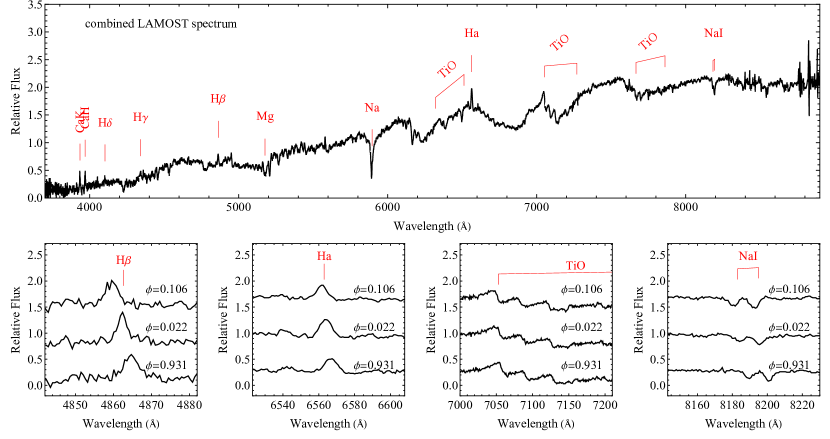
Supplementary Figure 1: The LAMOST low-resolution spectrum for J1123. Upper panel: the combined spectrum of LAMOST. Lower panels: zoom-in in the vicinity of ${\rm H\beta}$ 4863Å, ${\rm H\alpha}$ 6564Å, ${\rm TiO}$ 7050-7200Å, and ${\rm NaI}$ 8200Å (doublet), for three consecutive exposures taken by LAMOST on Feb 22, 2015.

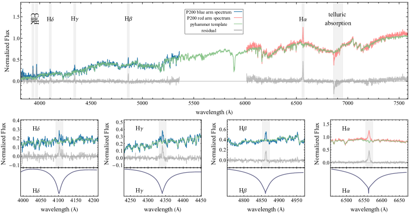
Supplementary Figure 2: The P200 spectrum for J1123. Upper panel: the P200 spectrum (the eighth exposure taken by DBSP on Mar 14, 2019; the mid-time of the exposure corresponds to the orbital phase $\phi$ $=$ 0.766) and the best-fit template. The spectrum is shifted to the rest-frame in vacuum. The best-fitted PyHammer template (green) has a spectral type $=$ M1 and metalicity $Z$ $=$ 0. Gray curve is the residual ($=$ observation $-$ template). Telluric absorption, Balmer emission lines, and Ca II H&K emission lines are shaded by shallow gray regions. Lower panels: zoom-in in the vicinity of ${\rm H\alpha}$, ${\rm H\beta}$, ${\rm H\gamma}$, and ${\rm H\delta}$. In the bottom sub-panels, the corresponding broad Balmer absorption lines of a theoretical WD spectrum^[93] (purple curve) with effective temperature $=$ 10000 K are shown for comparison. It is evident that no broad absorption feature of a WD is detected in our observations, as suggested by the residuals.

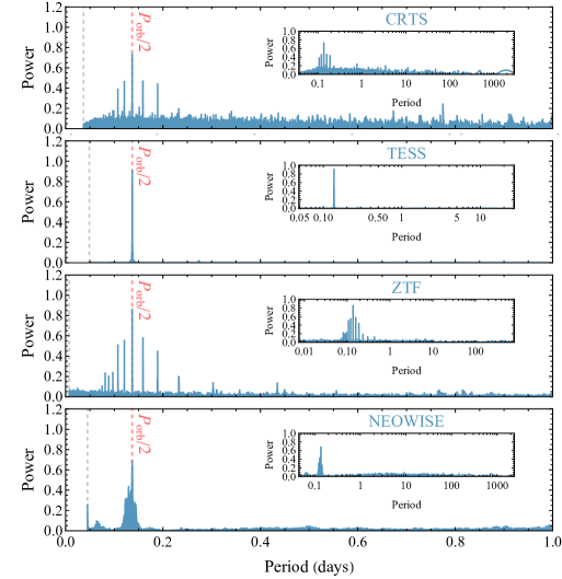
Supplementary Figure 3: The Lomb-Scargle powers of CRTS, TESS, ZTF r-band, and NEOWISE W1-band light curves (from top to bottom, respectively). The highest power (marked by the vertical red dashed lines) reports half the true orbital period of the ellipsoidal light curves. Vertical gray dashed lines mark the highest frequency of the period search grid, corresponding to a Nyquist factor $=$ 500 for CRTS, ZTF, and NEOWISE and a Nyquist factor $=$ 1 for TESS. The inset panel shows the power within the full searched period (frequency) window.

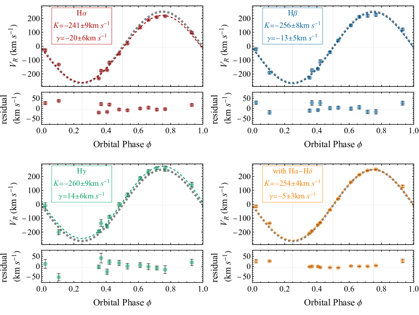
Supplementary Figure 4: The RV curves by fitting the H$\alpha$ (red), H$\beta$ (blue), H$\gamma$ (green) lines, and by fitting the full spectrum (orange) with all Balmer lines included. Data points refer to Supplementary Table 2 and error bars represent the $1$-sigma uncertainties. As for comparison, the gray dashed line in each panel is the RV curve obtained by fitting the full spectrum with all Balmer lines excluded (i.e., by fitting only the photospheric absorption lines of the M star).

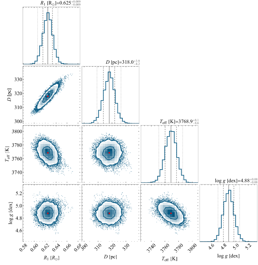
Supplementary Figure 5: The corner plot for the broadband SED fitting. The histograms indicate the marginal distributions for the fitted stellar parameters and the density plots indicate the joint distributions. In the histograms, the vertical dashed lines and the dotted lines represent the 1-sigma and the 2-sigma uncertainties, respectively.

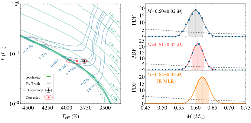
Supplementary Figure 6: The stellar properties of the visible M dwarf. Left panel: the position of J1123 in the HR diagram. Blue lines are the BT-Settl evolutionary tracks for stellar masses $M$ $=$ 0.45, 0.50, 0.57, 0.60, 0.62, 0.70, and 0.75$M_{\odot}$. Green lines are the isochrones at selected ages $=$ 0.001, 0.002, 0.005, 0.01, 0.02, 0.05, 0.1, 0.2, 0.5, 1, 2, 5, and 10 Gyrs. Note that the isochrones of 0.1-10 Gyrs almost lie on top of each other since M dwarfs do not move much once entering the main-sequence. The black dot is the SED derived (uncorrected) position of J1123 in the HR diagram, with error bars being the three-sigma uncertainties. The pink dot and ellipse are the corrected position and uncertainty by taking into account the influence of the tidal distortion effect. Right panels: the posterior distributions of the M dwarf’s mass, by using the uncorrected (SED derived; right upper panel) and the corrected $T_{\mathrm{eff}}$ (right middle panel), respectively. The posterior distributions (blue dots) are calculated by fitting the isochrones in 0.01 $M_{\odot}$ mass bins and fitted with a Gaussian (black and pink curves). The gray dashed line in each panel is the Kroupa initial mass function^[55], which is used as the prior. Also shown in the right lower panel is the mass inferred from the IR (2MASS Ks band) MLR^[60].

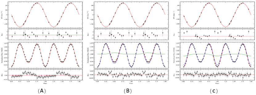
Supplementary Figure 7: PHOEBE’s best-fitting results. Upper panels: the best-fitting radial velocities (the red curve) versus the observations (the black dots) and the residuals (i.e., the differences between the fit and the data). Lower panels: the best-fitting flux variations (the red curve) versus the TESS observations (the black dots) and the residuals. The error bars correspond to the $1\sigma$ uncertainties. For model A (column A), we only consider the ellipsoidal modulations. It is evident that the light curve residuals show periodic variations. For model B (column B), The model light curve (the red curve) is a superposition of the ellipsoidal modulations (the blue curve) and a hotspot (the green curve). For model C (column C), the model light curve (the red curve) is superposition of the ellipsoidal modulations (the blue curve) and a coldspot (the green curve).

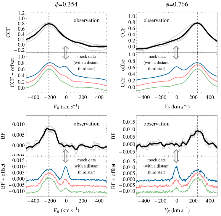
Supplementary Figure 8: The CCFs (top row) and the BFs (bottom row) for two P200 spectra at phases 0.354 (left column) and 0.766 (right column). Their corresponding RVs are indicated by the vertical dashed lines. For each panel, the upper sub-panel is the result of our P200 observations (black curve) obtained by averaging three shallow gray curves calculated using three different wavelength ranges (see Methods); the lower sub-panel is the result of the corresponding mock data in the case of a triple system. The blue, pink, and green curves represent the results for the case where the luminosity of the third star is 0.5, 0.2, and 0.1 times the luminosity of our visible M star, respectively (small vertical offsets are added for clarity). For the mock data, there is a prominent secondary peak from the third object in the CCF or the BF; such peak is absent in observations (indicated by the gray arrows). Thus a distant third object with luminosity $\gtrsim$ 0.1 times the luminosity of the M star can be safely ruled out.

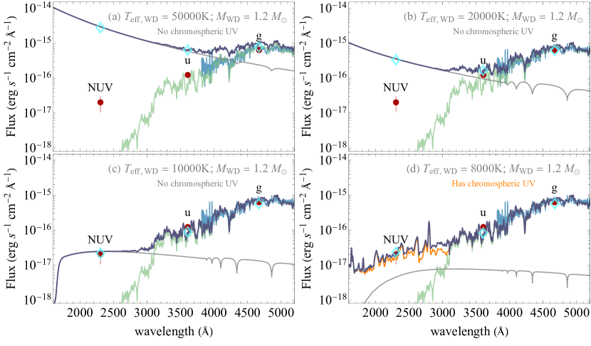
Supplementary Figure 9: Comparison of the P200 blue arm spectrum (light blue curve) with the composite SED (purple) of the M dwarf (green) plus a WD (gray). The observed photometry (red dots) and the synthetic photometry of the composite SED (cyan dimonds) are also shown for comparison. By using the known distance 318 pc, we scale on SED with four DA-type WD templates with the same mass ($M_{\mathrm{WD}}=1.2\ M_{\odot}$) and the same surface gravity ($\log{g}$ $=9.0$), but different temperatures (i.e., $T_{\mathrm{eff,WD}}=5\times 10^{4}$ K, $2\times 10^{4}$ K, $10^{4}$ K, and $8\times 10^{3}$ K). Only WDs with $T_{\mathrm{eff,WD}}$ $\lesssim 10^{4}$ K can well explain the observations. Panel (d) shows the realistic case, in which the composite SED also contains a substantial amount of chromospheric UV emission (orange curve; taken as the scaled mean spectrum of AD Leo and AU Mic for demonstration).

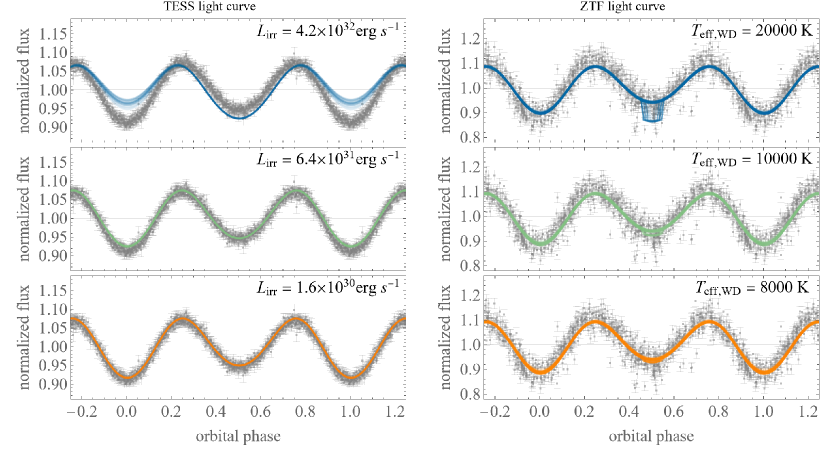
Supplementary Figure 10: Comparison of the PHOEBE simulated TESS light curves (left panels; coloured lines) and ZTF light curves (right panels; coloured lines) with the observations. Gray points are the observational data and the error bars represent the 1-sigma uncertainties. We use 100 sets of orbital parameters randomly drew from the distributions of the PHOEBE’s orbital solution to simulate each case described below. For the NS (left panels), three different irradiation luminosities: $4.2\times 10^{32}\ \mathrm{erg~{}s^{-1}}$, $6.4\times 10^{31}\ \mathrm{erg~{}s^{-1}}$, and $1.6\times 10^{30}\ \mathrm{erg~{}s^{-1}}$ are investigated. It is evident that for a NS with $L_{\rm irr}\gtrsim 6.4\times 10^{32}~{}\mathrm{erg~{}s^{-1}}$, the irradiation effect showing on the light curve is inconsistent with the TESS observations. Therefore we constrain the irradiation luminosity to be less than $6.4\times 10^{32}~{}\mathrm{erg~{}s^{-1}}$. For the WD (right panels), three different effective temperatures: 20000 K, 10000 K, and 8000 K are investigated. For a hot WD with $T_{\rm eff,~{}WD}$ = 20000 K, when the orbital inclination angle is large (nearly edge-on case), a prominent eclipse is expected at the M star’s inferior conjunction phase $\phi=0.5$; otherwise, there are no eclipses. For a WD with $T_{\rm eff,~{}WD}\lesssim 10000$ K, possible eclipse becomes hard to be identified given the photometric precision of our light curve. The simulation suggests that if the compact object in J1123 is a WD, the WD must be cold and massive.

References

- [1] Özel, F., Psaltis, D., Narayan, R. & Santos Villarreal, A. On the Mass Distribution and Birth Masses of Neutron Stars. ApJ 757, 55 (2012).
- [2] Keane, E. F. & Kramer, M. On the birthrates of Galactic neutron stars. MNRAS 391, 2009–2016 (2008).
- [3] Lorimer, D. R. Binary and Millisecond Pulsars. Living Reviews in Relativity 11, 8 (2008).
- [4] Abdo, A. A. et al. The First Fermi Large Area Telescope Catalog of Gamma-ray Pulsars. ApJS 187, 460–494 (2010).
- [5] Haberl, F. The magnificent seven: magnetic fields and surface temperature distributions. Ap&SS 308, 181–190 (2007).
- [6] Abbott, B. P. et al. GW170817: Observation of Gravitational Waves from a Binary Neutron Star Inspiral. Phys. Rev. Lett. 119, 161101 (2017).
- [7] Caraveo, P. A., Bignami, G. F. & Trümper, J. E. Radio-silent isolated neutron stars as a new astronomical reality. A&A Rev. 7, 209–216 (1996).
- [8] Cui, X.-Q. et al. The Large Sky Area Multi-Object Fiber Spectroscopic Telescope (LAMOST). Research in Astronomy and Astrophysics 12, 1197–1242 (2012).
- [9] Zhao, G., Zhao, Y.-H., Chu, Y.-Q., Jing, Y.-P. & Deng, L.-C. LAMOST spectral survey — An overview. Research in Astronomy and Astrophysics 12, 723–734 (2012).
- [10] Trimble, V. L. & Thorne, K. S. Spectroscopic Binaries and Collapsed Stars. ApJ 156, 1013 (1969).
- [11] Casares, J. et al. A Be-type star with a black-hole companion. Nature 505, 378–381 (2014).
- [12] Liu, J. et al. A wide star-black-hole binary system from radial-velocity measurements. Nature 575, 618–621 (2019).
- [13] Thompson, T. A. et al. A noninteracting low-mass black hole-giant star binary system. Science 366, 637–640 (2019).
- [14] Jayasinghe, T. et al. A unicorn in monoceros: the 3 M⊙ dark companion to the bright, nearby red giant V723 Mon is a non-interacting, mass-gap black hole candidate. MNRAS 504, 2577–2602 (2021).
- [15] Bailyn, C. D., Jain, R. K., Coppi, P. & Orosz, J. A. The Mass Distribution of Stellar Black Holes. ApJ 499, 367–374 (1998).
- [16] Morris, S. L. & Naftilan, S. A. The Equations of Ellipsoidal Star Variability Applied to HR 8427. ApJ 419, 344 (1993).
- [17] Kesseli, A. Y. et al. An Empirical Template Library of Stellar Spectra for a Wide Range of Spectral Classes, Luminosity Classes, and Metallicities Using SDSS BOSS Spectra. ApJS 230, 16 (2017).
- [18] Gaia Collaboration et al. Gaia Early Data Release 3. Summary of the contents and survey properties. A&A 649, A1 (2021).
- [19] Linsky, J. L. Stellar Model Chromospheres and Spectroscopic Diagnostics. ARA&A 55, 159–211 (2017).
- [20] Jones, D. O. & West, A. A. A Catalog of GALEX Ultraviolet Emission from Spectroscopically Confirmed M Dwarfs. ApJ 817, 1 (2016).
- [21] Roberts, M. S. E. Surrounded by spiders! New black widows and redbacks in the Galactic field. In van Leeuwen, J. (ed.) Neutron Stars and Pulsars: Challenges and Opportunities after 80 years, vol. 291, 127–132 (2013).
- [22] Burdge, K. B. et al. A 62-minute orbital period black widow binary in a wide hierarchical triple. Nature 605, 41–45 (2022).
- [23] Polzin, E. J. et al. Study of spider pulsar binary eclipses and discovery of an eclipse mechanism transition. MNRAS 494, 2948–2968 (2020).
- [24] Hessels, J. W. T. et al. A Radio Pulsar Spinning at 716 Hz. Science 311, 1901–1904 (2006).
- [25] Clark, C. J. et al. Einstein@Home discovery of the gamma-ray millisecond pulsar PSR J2039-5617 confirms its predicted redback nature. MNRAS 502, 915–934 (2021).
- [26] The Fermi-LAT collaboration et al. Fermi Large Area Telescope Fourth Source Catalog. ApJS 247, 33 (2020).
- [27] Johnston, S. et al. Discovery of a very bright, nearby binary millisecond pulsar. Nature 361, 613–615 (1993).
- [28] Verbunt, F. & Zwaan, C. Magnetic braking in low-mass X-ray binaries. A&A 100, L7–L9 (1981).
- [29] Rappaport, S., Verbunt, F. & Joss, P. C. A new technique for calculations of binary stellar evolution application to magnetic braking. ApJ 275, 713–731 (1983).
- [30] Shao, Y. & Li, X.-D. Formation and Evolution of Galactic Intermediate/Low-Mass X-ray Binaries. ApJ 809, 99 (2015).

References

- [1] Bai, Z.-R. et al. The first data release of LAMOST low-resolution single-epoch spectra. Research in Astronomy and Astrophysics 21, 249 (2021).
- [2] Drake, A. J. et al. The Catalina Surveys Periodic Variable Star Catalog. ApJS 213, 9 (2014).
- [3] Mu, H.-J. et al. Compact object candidates with K/M-dwarf companions from LAMOST low-resolution survey. Science China Physics, Mechanics, and Astronomy 65, 229711 (2022).
- [4] Bellm, E. C. et al. The Zwicky Transient Facility: System Overview, Performance, and First Results. PASP 131, 018002 (2019).
- [5] Mainzer, A. et al. Preliminary Results from NEOWISE: An Enhancement to the Wide-field Infrared Survey Explorer for Solar System Science. ApJ 731, 53 (2011).
- [6] Ricker, G. R. et al. Transiting Exoplanet Survey Satellite (TESS). Journal of Astronomical Telescopes, Instruments, and Systems 1, 014003 (2015).
- [7] Lightkurve Collaboration et al. Lightkurve: Kepler and TESS time series analysis in Python. Astrophysics Source Code Library (2018).
- [8] Lomb, N. R. Least-Squares Frequency Analysis of Unequally Spaced Data. Ap&SS 39, 447–462 (1976).
- [9] Scargle, J. D. Studies in astronomical time series analysis. II. Statistical aspects of spectral analysis of unevenly spaced data. ApJ 263, 835–853 (1982).
- [10] Zechmeister, M. & Kürster, M. The generalised Lomb-Scargle periodogram. A new formalism for the floating-mean and Keplerian periodograms. A&A 496, 577–584 (2009).
- [11] Press, W. H. & Rybicki, G. B. Fast Algorithm for Spectral Analysis of Unevenly Sampled Data. ApJ 338, 277 (1989).
- [12] VanderPlas, J. T. Understanding the Lomb-Scargle Periodogram. ApJS 236, 16 (2018).
- [13] Martin, D. C. et al. The Galaxy Evolution Explorer: A Space Ultraviolet Survey Mission. ApJ 619, L1–L6 (2005).
- [14] York, D. G. et al. The Sloan Digital Sky Survey: Technical Summary. AJ 120, 1579–1587 (2000).
- [15] Chambers, K. C. et al. The Pan-STARRS1 Surveys. arXiv e-prints arXiv:1612.05560 (2016).
- [16] Cutri, R. M. et al. VizieR Online Data Catalog: 2MASS All-Sky Catalog of Point Sources (Cutri+ 2003). VizieR Online Data Catalog II/246 (2003).
- [17] Wright, E. L. et al. The Wide-field Infrared Survey Explorer (WISE): Mission Description and Initial On-orbit Performance. AJ 140, 1868–1881 (2010).
- [18] Cutri, R. M. & et al. VizieR Online Data Catalog: WISE All-Sky Data Release (Cutri+ 2012). VizieR Online Data Catalog II/311 (2012).
- [19] Green, G. M. et al. Galactic reddening in 3D from stellar photometry - an improved map. MNRAS 478, 651–666 (2018).
- [20] El-Badry, K. et al. LAMOST J0140355 + 392651: an evolved cataclysmic variable donor transitioning to become an extremely low-mass white dwarf. MNRAS 505, 2051–2073 (2021).
- [21] Cardelli, J. A., Clayton, G. C. & Mathis, J. S. The Relationship between Infrared, Optical, and Ultraviolet Extinction. ApJ 345, 245 (1989).
- [22] Fitzpatrick, E. L. Correcting for the Effects of Interstellar Extinction. PASP 111, 63–75 (1999).
- [23] Allard, F., Homeier, D. & Freytag, B. Models of very-low-mass stars, brown dwarfs and exoplanets. Philosophical Transactions of the Royal Society of London Series A 370, 2765–2777 (2012).
- [24] Bayo, A. et al. VOSA: virtual observatory SED analyzer. An application to the Collinder 69 open cluster. A&A 492, 277–287 (2008).
- [25] Kroupa, P. On the variation of the initial mass function. MNRAS 322, 231–246 (2001).
- [26] Feiden, G. A. & Chaboyer, B. Magnetic Inhibition of Convection and the Fundamental Properties of Low-mass Stars. I. Stars with a Radiative Core. ApJ 779, 183 (2013).
- [27] Parker, E. N. Hydromagnetic Dynamo Models. ApJ 122, 293 (1955).
- [28] Morgan, D. P. et al. The Effects of Close Companions (and Rotation) on the Magnetic Activity of M Dwarfs. AJ 144, 93 (2012).
- [29] Kraus, A. L., Tucker, R. A., Thompson, M. I., Craine, E. R. & Hillenbrand, L. A. The Mass-Radius(-Rotation?) Relation for Low-mass Stars. ApJ 728, 48 (2011).
- [30] Benedict, G. F. et al. The Solar Neighborhood. XXXVII: The Mass-Luminosity Relation for Main-sequence M Dwarfs. AJ 152, 141 (2016).
- [31] Prša, A. & Zwitter, T. A Computational Guide to Physics of Eclipsing Binaries. I. Demonstrations and Perspectives. ApJ 628, 426–438 (2005).
- [32] Prša, A. et al. Physics Of Eclipsing Binaries. II. Toward the Increased Model Fidelity. ApJS 227, 29 (2016).
- [33] Conroy, K. E. et al. Physics of Eclipsing Binaries. V. General Framework for Solving the Inverse Problem. ApJS 250, 34 (2020).
- [34] Claret, A. Limb and gravity-darkening coefficients for the TESS satellite at several metallicities, surface gravities, and microturbulent velocities. A&A 600, A30 (2017).
- [35] Morris, S. L. The ellipsoidal variable stars. ApJ 295, 143–152 (1985).
- [36] Gomel, R., Faigler, S. & Mazeh, T. Search for dormant black holes in ellipsoidal variables I. Revisiting the expected amplitudes of the photometric modulation. MNRAS 501, 2822–2832 (2021).
- [37] Rowan, D. M. et al. High tide: a systematic search for ellipsoidal variables in ASAS-SN. MNRAS 507, 104–115 (2021).
- [38] Foreman-Mackey, D., Hogg, D. W., Lang, D. & Goodman, J. emcee: The MCMC Hammer. PASP 125, 306 (2013).
- [39] Merle, T. et al. The Gaia-ESO Survey: double-, triple-, and quadruple-line spectroscopic binary candidates. A&A 608, A95 (2017).
- [40] Clark Cunningham, J. M. et al. APOGEE/Kepler Overlap Yields Orbital Solutions for a Variety of Eclipsing Binaries. AJ 158, 106 (2019).
- [41] Traven, G. et al. The GALAH survey: multiple stars and our Galaxy. I. A comprehensive method for deriving properties of FGK binary stars. A&A 638, A145 (2020).
- [42] Kounkel, M. et al. Double-lined Spectroscopic Binaries in the APOGEE DR16 and DR17 Data. AJ 162, 184 (2021).
- [43] Li, C.-q. et al. Double- and Triple-line Spectroscopic Candidates in the LAMOST Medium-Resolution Spectroscopic Survey. ApJS 256, 31 (2021).
- [44] Tonry, J. & Davis, M. A survey of galaxy redshifts. I. Data reduction techniques. AJ 84, 1511–1525 (1979).
- [45] Rucinski, S. M. Spectral-Line Broadening Functions of WUMa-Type Binaries. I. AW UMa. AJ 104, 1968 (1992).
- [46] Rucinski, S. Determination of Broadening Functions Using the Singular-Value Decomposition (SVD) Technique. In Hearnshaw, J. B. & Scarfe, C. D. (eds.) IAU Colloq. 170: Precise Stellar Radial Velocities, vol. 185 of Astronomical Society of the Pacific Conference Series, 82 (1999).
- [47] Gray, D. F. The Observation and Analysis of Stellar Photospheres (2005).
- [48] Lindegren, L. et al. Gaia Early Data Release 3. The astrometric solution. A&A 649, A2 (2021).
- [49] Gandhi, P. et al. Astrometric excess noise in Gaia EDR3 and the search for X-ray binaries. MNRAS 510, 3885–3895 (2022).
- [50] Belokurov, V. et al. Unresolved stellar companions with Gaia DR2 astrometry. MNRAS 496, 1922–1940 (2020).
- [51] Bai, Y. et al. The UV Emission of Stars in the LAMOST Survey. I. Catalogs. ApJS 235, 16 (2018).
- [52] Boggess, A. et al. The IUE spacecraft and instrumentation. Nature 275, 372–377 (1978).
- [53] Boggess, A. et al. In-flight performance of the IUE. Nature 275, 377–385 (1978).
- [54] Rugheimer, S., Kaltenegger, L., Segura, A., Linsky, J. & Mohanty, S. Effect of UV Radiation on the Spectral Fingerprints of Earth-like Planets Orbiting M Stars. ApJ 809, 57 (2015).
- [55] Hotan, A. W., van Straten, W. & Manchester, R. N. PSRCHIVE and PSRFITS: An Open Approach to Radio Pulsar Data Storage and Analysis. PASA 21, 302–309 (2004).
- [56] Cordes, J. M. & Lazio, T. J. W. NE2001.I. A New Model for the Galactic Distribution of Free Electrons and its Fluctuations. arXiv e-prints astro–ph/0207156 (2002).
- [57] Yao, J. M., Manchester, R. N. & Wang, N. A New Electron-density Model for Estimation of Pulsar and FRB Distances. ApJ 835, 29 (2017).
- [58] Ransom, S. M. New search techniques for binary pulsars. Ph.D. thesis, Harvard University (2001).
- [59] Andersen, B. C. & Ransom, S. M. A Fourier Domain “Jerk” Search for Binary Pulsars. ApJ 863, L13 (2018).
- [60] Wang, P. et al. FAST discovery of an extremely radio-faint millisecond pulsar from the Fermi-LAT unassociated source 3FGL J0318.1+0252. Science China Physics, Mechanics, and Astronomy 64, 129562 (2021).
- [61] Jurić, M. et al. The Milky Way Tomography with SDSS. I. Stellar Number Density Distribution. ApJ 673, 864–914 (2008).
- [62] Bensby, T., Feltzing, S. & Lundström, I. Elemental abundance trends in the Galactic thin and thick disks as traced by nearby F and G dwarf stars. A&A 410, 527–551 (2003).
- [63] Koester, D. White dwarf spectra and atmosphere models. Mem. Soc. Astron. Italiana 81, 921–931 (2010).
- [64] Parsons, S. G. et al. Magnetic white dwarfs in post-common-envelope binaries. MNRAS 502, 4305–4327 (2021).
- [65] Liebert, J. et al. Where Are the Magnetic White Dwarfs with Detached, Nondegenerate Companions? AJ 129, 2376–2381 (2005).
- [66] Schreiber, M. R., Belloni, D., Gaensicke, B. T., Parsons, S. G. & Zorotovic, M. The origin and evolution of magnetic white dwarfs in close binary stars. Nature Astronomy 5, 648-654 (2021).
- [67] Breton, R. P. et al. Discovery of the Optical Counterparts to Four Energetic Fermi Millisecond Pulsars. ApJ 769, 108 (2013).
- [68] Anders, F. et al. Photo-astrometric distances, extinctions, and astrophysical parameters for Gaia EDR3 stars brighter than G = 18.5. A&A 658, A91 (2022).
- [69] Henry, T. J., Kirkpatrick, J. D. & Simons, D. A. The Solar Neighborhood. I. Standard Spectral Types (K5-M8) for Northern Dwarfs Within Eight Parsecs. AJ 108, 1437 (1994).
- [70] Favata, F., Micela, G. & Reale, F. The corona of the dMe flare star AD Leo. A&A 354, 1021–1035 (2000).
- [71] Walkowicz, L. M., Johns-Krull, C. M. & Hawley, S. L. Characterizing the Near-UV Environment of M Dwarfs. ApJ 677, 593–606 (2008).
- [72] Reid, I. N., Hawley, S. L. & Gizis, J. E. The Palomar/MSU Nearby-Star Spectroscopic Survey. I. The Northern M Dwarfs -Bandstrengths and Kinematics. AJ 110, 1838 (1995).
- [73] Jones, H. R. A., Longmore, A. J., Allard, F. & Hauschildt, P. H. Spectral analysis of M dwarfs. MNRAS 280, 77–94 (1996).
- [74] Walkowicz, L. M. & Hawley, S. L. Tracers of Chromospheric Structure. I. Observations of Ca II K and H in M Dwarfs. AJ 137, 3297–3313 (2009).
- [75] Torres, C. A. O. et al. Search for associations containing young stars (SACY). I. Sample and searching method. A&A 460, 695–708 (2006).
- [76] Plavchan, P. et al. A planet within the debris disk around the pre-main-sequence star AU Microscopii. Nature 582, 497–500 (2020).
- [77] White, R. J. et al. Stellar Radius Measurements of the Young Debris Disk Host AU Mic. In American Astronomical Society Meeting Abstracts #225, vol. 225 of American Astronomical Society Meeting Abstracts, 348.12 (2015).
- [78] Plavchan, P. et al. New Debris Disks Around Young, Low-Mass Stars Discovered with the Spitzer Space Telescope. ApJ 698, 1068–1094 (2009).