Lightweight Image Codec via Multi-Grid Multi-Block-Size Vector Quantization (MGBVQ)

Abstract

A multi-grid multi-block-size vector quantization (MGBVQ) method is proposed for image coding in this work. The fundamental idea of image coding is to remove correlations among pixels before quantization and entropy coding, e.g., the discrete cosine transform (DCT) and intra predictions, adopted by modern image coding standards. We present a new method to remove pixel correlations. First, by decomposing correlations into long- and short-range correlations, we represent long-range correlations in coarser grids due to their smoothness, thus leading to a multi-grid (MG) coding architecture. Second, we show that short-range correlations can be effectively coded by a suite of vector quantizers (VQs). Along this line, we argue the effectiveness of VQs of very large block sizes and present a convenient way to implement them. It is shown by experimental results that MGBVQ offers excellent rate-distortion (RD) performance, which is comparable with existing image coders, at much lower complexity. Besides, it provides a progressive coded bitstream.

I Introduction

Image coding has been studied for more than four decades. Many image coding standards have been finalized and widely used today, e.g., JPEG [1] and intra coding of many video coding standards, e.g., H.264 intra [2], Webp [3] from VP8 intra [4], BPG [5] from HEVC intra [6], AV1 intra [7] and VVC intra [8]. To achieve higher and higher coding gains, the coding standards become more and more complicated by including computationally intensive units like intra prediction, flexible coding block partition and more transform types. Specialized hardware are developed to reduce the coding time [9, 10].

Another new development is the emergence of learning-based image coding solutions [11, 12]. Image coding methods based on deep learning [13] have received a lot of attention in recent years, due to their impressive coding gain. For example, Balle et. al [14] used the variational autoencoder (VAE) [15], generalized divisive normalization (GDN) [16], the hyper-prior model [17] and a carefully designed quantization scheme to train an end-to-end optimized image codec. Recent work on deep-learning-based (DL-based) image/video coding achieves nice results and were reviewed in [18, 19].

Recent image coding RnD activities have focused on rate-distortion (RD) [20, 21] performance improvement at the expense of higher complexity. Here, we pursue another direction by looking for a lightweight image codec even at the cost of slightly lower RD performance. In particular, we revisit a well-known learning-based image coding solution, i.e., vector quantization (VQ). There has been a long history of VQ research [22] and its application to image coding [23, 24, 25]. Yet, VQ-based image codec has never become mainstream. To make VQ a strong competitor, it is essential to cast it in a new framework.

A multi-grid multi-block-size vector quantization (MGBVQ) method is proposed for image coding in this work. The fundamental idea of image coding is to remove correlations among pixels before quantization and entropy coding. For example, DCT and intra predictions are adopted by modern image coding standards to achieve this objective. To remove pixel correlations, our first idea is to decompose pixel correlations into long- and short-range correlations. Long-range correlations can be represented by coarser grids since they are smoother. Recursive application of this idea leads to a multi-grid (MG) coding architecture. Our second idea is to encode short-range pixel correlations by a suite of vector quantizers (VQs). Along this line, we argue the effectiveness of VQs of very large block sizes and present a convenient way to implement them. Experiments demonstrate that MGBVQ offers an excellent rate-distortion (RD) performance that is comparable with state-of-the-art image coders at much lower complexity.

Furthermore, progressive coding [26, 27] is a desired functionality of an image codec. For example, JPEG has a progressive mode. JPEG-2000 [28] also supports progressive coding. H.264/SVC offers a scalable counterpart of H.264/AVC [29], which is achieved by sacrificing the RD performance [30]. We will show that MGBVQ offers a progressive coding bitstream by nature.

The rest of this paper is organized as follows. The MGBVQ method is introduced in Sec. II. Experimental results are shown in Sec. III. Concluding remarks and future research directions are pointed out in Sec. IV.

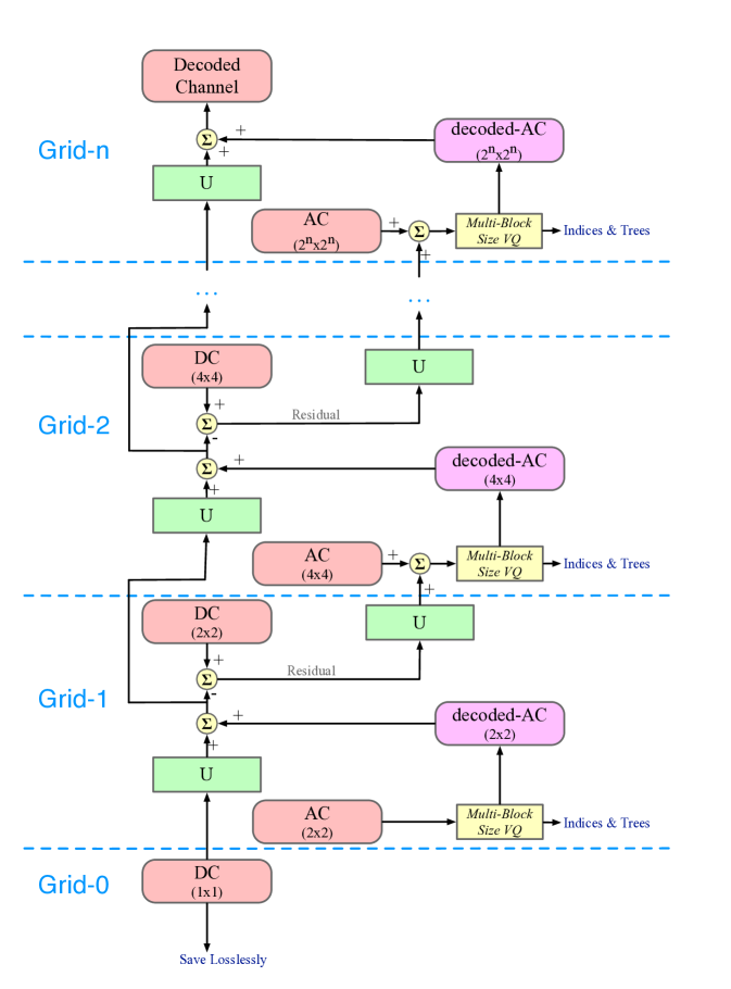
Figure 1: An overview of the proposed MGBVQ method.

II MGBVQ Method

II-A Multi-Grid (MG) Representation

To encode/decode images of spatial resolution $2^{N}\times 2^{N}$, we build a sequence of grids, $G_{n}$, of spatial resolution $2^{n}\times 2^{n}$, where $n=1,\cdots,N$, to represent them as shown in Fig. 1. To achieve this goal, we begin with an image, $I_{N}$, at the finest grid $G_{N}$. We decompose it into a smooth component and a residual component. The latter is the difference between the original signal and the smooth component. For convenience, the smooth and the residual components are called DC and AC components for the rest of this paper. Since the DC component is smooth, we downsample it using the Lanczos operator [31] and represent it in grid $G_{N-1}$. Mathematically, this can be written as

$$I_{N-1}=D(I_{N}),$$ (1)

where $D$ denotes the downsampling operation from $G_{N}$ to $G_{N-1}$. Similarly, we can upsample image $I_{N-1}$ to $I_{N}$ via

$$\tilde{I}_{N}=U(I_{N-1})=U[D(I_{N})].$$ (2)

where the upsampling operation, $U$, is also implemented by the Lanczos operator. Then, the AC component can be computed by

$$AC_{N}=I_{N}-\tilde{I}_{N}=I_{N}-U[D(I_{N})].$$ (3)

The above decomposition process can be repeated for $I_{N-1}$, $I_{N-2}$, up to $I_{2}$. Then, grid $G_{n}$ is used to represent $AC_{n}$, where $n=N,N-1,\cdots,2$ while grid $G_{0}$ is used to represent $DC_{0}$ in the MG image representation.

It is worthwhile to comment that all existing image/video coding standards adopt the single-grid representation. The difference between smooth and textured/edged regions is handled by block partitioning with different block sizes. Yet, there are low-frequency components in textured/edged regions and partitioning these regions into smaller blocks has a negative impact on exploiting long-range pixel correlations, which can be overcome by the MG representation. Another advantage of the MG representation is its effectiveness in the RD performance. Suppose that grid $G_{n}$ pays the cost of one bit per pixel (bpp) to reduce a certain amount of mean-squared error (MSE) denoted by $\Delta MSE$. The cost becomes $4^{n-N}$ bpp at grid $G_{N}$ since the MSE reduction is shared by $4^{N-n}$ pixels.

TABLE I: Parameter setting for $256\times 256$ images, where we specify the number of codewords and the number of spectral components in codebook $C_{n,m}$ by (#codeword, #components). For $C_{8,3}$, we have $N\in\{8,16,32,64,128\}$ which gives the 5 points in Fig. 5(a)

	$G_{8}$	$G_{7}$	$G_{6}$	$G_{5}$	$G_{4}$	$G_{3}$
$C_{*,8}$	(64,150)	-	-	-	-	-
$C_{*,7}$	(128,150)	(64,150)	-	-	-	-
$C_{*,6}$	(512,150)	(128,150)	(64,100)	-	-	-
$C_{*,5}$	(512,50)	(512,50)	(128,40)	(64,40)	-	-
$C_{*,4}$	(512,30)	(512,30)	(512,20)	(128,20)	(64,20)	-
$C_{*,3}$	(N,-)	(512,20)	(512,12)	(512,12)	(32,12)	(64,12)
$C_{*,2}$	-	(128,-)	(512,-)	(512,-)	(64,-)	(32,-)

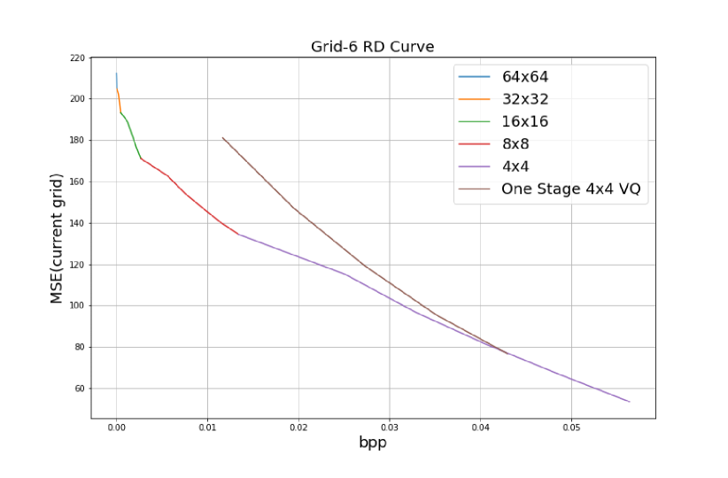
(a) $G_{6}$ RD curve

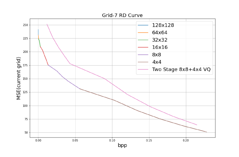
(b) $G_{7}$ RD curve

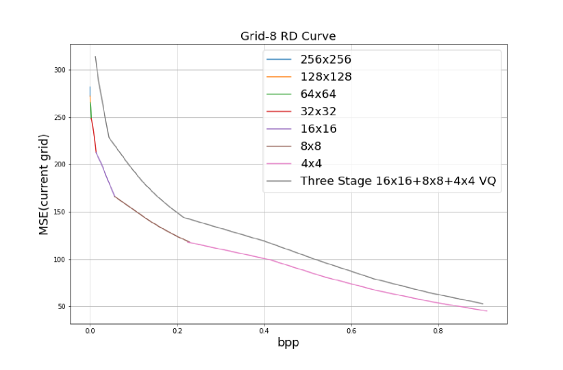
(c) $G_{8}$ RD curve

Figure 2: The RD curves for grids $G_{6}$, $G_{7}$ and $G_{8}$, which are benchmarked with one-stage, two-stage and three-stage VQ designs.

II-B Multi-Block-Size VQ

We use VQ to encode AC components in grids $G_{n}$, $n=2,\cdots,N$. Our proposed VQ scheme has several salient features as compared with the traditional VQ. That is, multiple codebooks of different block sizes (or codeword sizes) are trained at each grid. The codebooks are denoted by $C_{n,m}$, where subscripts $n$ and $m$ indicate the index of grid $G_{n}$ and the codeword dimension ($2^{m}\times 2^{m}$), respectively. We have $m\leq n$ since the codeword dimension is upper bounded by the grid dimension. We use $|C_{n,m}|$ to denote the number of codewords in $C_{n,m}$.

At grid $G_{n}$, we begin with codebook $C_{n,n}$ of the largest codeword size, where the codeword size is the same as the grid size. As a result, the AC component can be coded by one codeword from the codebook $C_{n,n}$. After that, we compute the residual between the original and the $C_{n,n}$-quantized AC images, partition it into four non-overlapping regions, and encode each region with a codeword from codebook $C_{n,n-1}$. This process is repeated until the codeword size is sufficiently small with respect to the target grid.

Before proceeding, it is essential to answer the following several questions:

• Q1: How to justify this design?

• Q2: How to train VQ codebooks of large codeword sizes? How to encode an input AC image with trained VQ codebooks at Grid $G_{n}$?

• Q3: How to determine codebook size $|C_{n,m}|$?

• Q4: When to switch from codebook $C_{n,m}$ to codebook $C_{n,m-1}$?

VQ learns the distribution of samples in a certain space, denoted by $R^{L}$, and finds a set of representative ones as codewords. The error between a sample and its representative one has to be normalized by dimension $L$. If there is an upper bound of the average error (i.e. the MSE), a larger $L$ value is favored. On the other hand, there is also a lower bound on the average error since the code size cannot be too large (due to worse RD performance). To keep good RD performance, we should switch from codebook $C_{n,m}$ to codebook $C_{n,m-1}$. Actually, Q1, Q3 and Q4 can be answered rigorously using the RD analysis. This will be presented in an extended version of this paper. Some RD results of codebooks of different codeword sizes are shown in the experimental section.

To answer Q2, we transform an image block of sizes $2^{m}\times 2^{m}$ from the spatial domain to the spectral domain via a sequence of cascaded channel-wise (c/w) Saab transforms [32]. The c/w Saab transform is a variant of the principal component analysis (PCA). However, a single-stage PCA is difficult to apply for large $m$. Instead, we group small non-overlapping blocks (say, of size $2\times 2$) and conduct the transform locally. Then, we discard channels of low response values and keep channels of high response values for dimension reduction. Finally, we are able to reach the final stage that has only a spatial dimension of $1\times 1$ of $K$ spectral components. The combination of multi-stage local filtering and dimension reduction allows the spectral analysis of any blocks of large sizes. All transform parameters are learned from the data. We train codebook $C_{n,n}$ based on clustering of $K$ components in the spectral domain. After quantization, we can transform the quantized codeword back to the spatial domain via the inverse c/w Saab transform. This can be implemented as a look-up table since it has to be done only once. Then, we can compute the AC residual by subtracting the quantized AC value from the original AC value.

There are miscellaneous coding tools used. First, for color image coding, it is observed that the c/w Saab transform can compact energy well in the spatial domain as well as R, G, B three channels. Thus, when we train VQ codebooks $C_{n,m}$, we simply consider codewords of dimension $2^{m}\times 2^{m}\times 3$. Second, the simple Huffman coder is adopted as the entropy coder. The codeword indices of each codebook $C_{n,m}$ are coded using a Huffman table learned from training data. Third, it is advantageous to adopt different codebooks in different spatial regions at finer grids. For example, we can switch to codebooks of smaller block sizes in complex regions while stay with codebooks of larger blocks in simple regions. This is a rate control problem. We implement rate control using a quad-tree. If a region is smooth, there is no need to switch to codebooks of smaller code sizes. This is called early termination. Early termination helps reduce the number of bits a lot in finer grids. For example, without early termination, the coding of Lena of resolution $256\times 256$ at $G_{8}$ with $C_{8,8}$, which has 64 codewords, needs 0.09bpp. Early termination with entropy coding can reduce it to 0.0246bpp.

(a) H.264-444 $21.38dB@0.2447bpp$

(b) JPEG Progressive $22.21dB@0.2355bpp$

(c) BPG-444 $28.84dB@0.2520bpp$

(d) Our Method $26.29dB@0.2452bpp$

Figure 3: Evaluation results for Lena of resolution $256\times 256$.

(a) H.264-444 $25.79dB@0.1176bpp5$

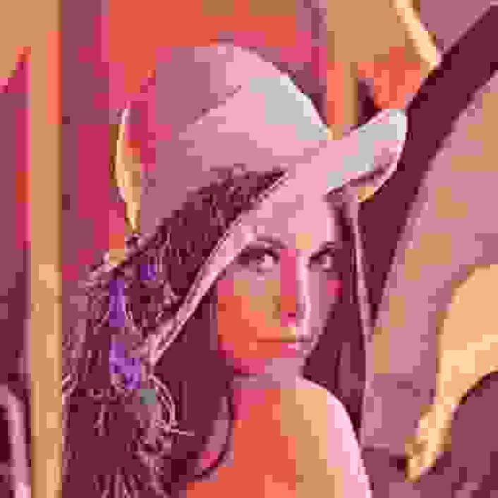
(b) JPEG Progressive $21.29dB@0.1176bpp$

(c) BPG-444 $29.72dB@0.1191bpp$

(d) Our Method $27.18dB@0.1194bpp$

Figure 4: Evaluation results for Lena of resolution $512\times 512$.

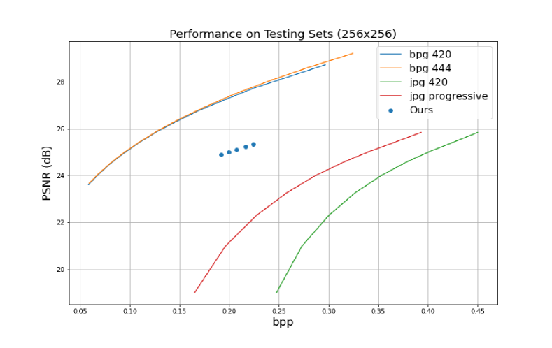
(a) Scale: $256\times 256$

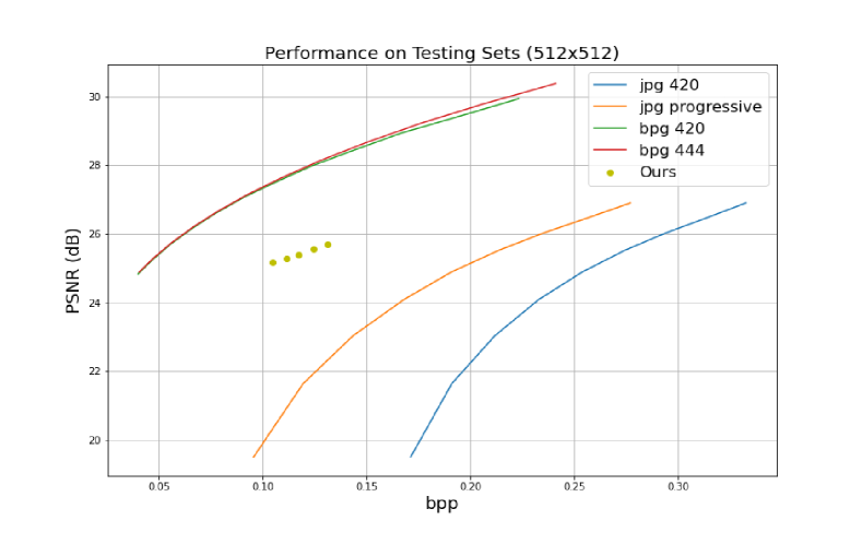
(b) Scale: $512\times 512$

Figure 5: Evaluation results on the average of 186 test images.

TABLE II: Bit rate distribution as a function of the block size at each grid for Lena ($256\times 256$, $26.19dB@0.2286bpp$), where QT stands for the cost of saving the quad-tree at each grid. Only DC in $G_{2}$ is coded. Other numbers in the first column show the block size and ”-” means either no bit needed or not applicable.

	$G_{8}$	$G_{7}$	$G_{6}$	$G_{5}$	$G_{4}$	$G_{3}$	$G_{2}$
QT	4.0e-3	4.8e-3	1.3e-3	3.2e-4	7.6e-5	1.5e-5	-
DC	-	-	-	-	-	-	2.4e-4
$C_{*,8}$	1.5e-5	-	-	-	-	-	-
$C_{*,7}$	9.1e-5	1.5e-5	-	-	-	-	-
$C_{*,6}$	7.6e-4	1.5e-4	1.5e-5	-	-	-	-
$C_{*,5}$	5.1e-3	1.2e-3	1.6e-5	7.6e-5	-	-	-
$C_{*,4}$	0.0213	7.2e-3	1.7e-3	3.1e-4	6.1e-5	-	-
$C_{*,3}$	0.0246	0.029	8.2e-3	2.1e-3	3.2e-4	7.6e-5
$C_{*,2}$	-	0.073	0.0322	8.6e-3	1.5e-3	3.2e-4	-

III Experiments

In the experiments, we use images from the CLIC training set [33] and Holopix50k [34] as training ones, use Lena and CLIC test images as test ones. Except for Lena, which is of resolution $512\times 512$, we crop images of resolution $1024\times 1024$ with stride 512 from the original high resolution images to serve as training and test images. To verify the progressive characteristics, we down-sample images of resolution $1024\times 1024$ to $512\times 512$ and $256\times 256$ using the Lanczos interpolation. There are 186 test images in total.

We select 3400 images from the training set to train VQ codebooks. They are trained by the faiss.KMeans method [35], which provides a multi-thread implementation. Fig. 2 shows multiple codebooks $C_{n,m}$ at grids $G_{n}$ in terms of the number of codewords and the number of the kept spectral components in the final stage in VQ training which results the parameters we used shown in TABLE.I.

Figs. 3 and 4 compare decoded images from several standards and our MGBVQ method at the same bit rate of resolutions $256\times 256$ and $512\times 512$, respectively. Figs. 5(a) and 5(b) compare the averaged RD performance for 186 test images of resolutions $256\times 256$ and $512\times 512$, respectively. We see from these figures that MGBVQ achieves remarkable performance under a very simple framework without any post-processing. More textures are retained by our framework since the traditional transform coding scheme tends to discard high frequencies to achieve more zeros especially when the bit rate is low. While in our framework, high frequencies are captured by larger grid VQ and smaller block VQ when necessary.

The distribution of bits spent in coding at each grid is summarized in Table II. We see from the table that the coding of DC and VQ indices in coarse grids account for a small percentage of the total bit rate . The great majority of bits are spent in the finest grid and smallest block sizes, say, the coding of indices of codebooks $C_{8,3}$, $C_{7,2}$, $C_{7,3}$ and $C_{6,2}$.

IV Conclusion and Future Work

A lightweight learning-based image codec, called MGBVQ, was proposed in this work. Its feasibility and potential has been demonstrated by experimental results. However, there are a few details that can be fine-tuned, including rate control and entropy coding. We will continue to push its performance and demonstrate that the new framework will achieve competitive performance as compared with deep-learning-based image coding method at much lower computational complexity.

References

- [1] G. K. Wallace, “The jpeg still picture compression standard,” IEEE transactions on consumer electronics, vol. 38, no. 1, pp. xviii–xxxiv, 1992.
- [2] T. Wiegand, G. J. Sullivan, G. Bjontegaard, and A. Luthra, “Overview of the h. 264/avc video coding standard,” IEEE Transactions on circuits and systems for video technology, vol. 13, no. 7, pp. 560–576, 2003.
- [3] L. Lian and W. Shilei, “Webp: A new image compression format based on vp8 encoding,” Microcontrollers & Embedded Systems, vol. 3, 2012.
- [4] J. Bankoski, P. Wilkins, and Y. Xu, “Technical overview of vp8, an open source video codec for the web,” in 2011 IEEE International Conference on Multimedia and Expo. IEEE, 2011, pp. 1–6.
- [5] Better Portable Graphics. [Online]. Available: https://bellard.org/bpg/
- [6] G. J. Sullivan, J.-R. Ohm, W.-J. Han, and T. Wiegand, “Overview of the high efficiency video coding (hevc) standard,” IEEE Transactions on circuits and systems for video technology, vol. 22, no. 12, pp. 1649–1668, 2012.
- [7] Y. Chen, D. Murherjee, J. Han, A. Grange, Y. Xu, Z. Liu, S. Parker, C. Chen, H. Su, U. Joshi et al., “An overview of core coding tools in the av1 video codec,” in 2018 Picture Coding Symposium (PCS). IEEE, 2018, pp. 41–45.
- [8] Y.-K. Wang, R. Skupin, M. M. Hannuksela, S. Deshpande, V. Drugeon, R. Sjöberg, B. Choi, V. Seregin, Y. Sanchez, J. M. Boyce et al., “The high-level syntax of the versatile video coding (vvc) standard,” IEEE Transactions on Circuits and Systems for Video Technology, 2021.
- [9] U. Albalawi, S. P. Mohanty, and E. Kougianos, “A hardware architecture for better portable graphics (bpg) compression encoder,” in 2015 IEEE International Symposium on Nanoelectronic and Information Systems. IEEE, 2015, pp. 291–296.
- [10] M. Elbadri, R. Peterkin, V. Groza, D. Ionescu, and A. El Saddik, “Hardware support of jpeg,” in Canadian Conference on Electrical and Computer Engineering, 2005. IEEE, 2005, pp. 812–815.
- [11] J. Yang, G. Zhu, J. Huang, and X. Zhao, “Estimating jpeg compression history of bitmaps based on factor histogram,” Digital Signal Processing, vol. 41, pp. 90–97, 2015.
- [12] J. Yang, C. Yang, Y. Ma, S. Liu, and R. Wang, “Learned low bit-rate image compression with adversarial mechanism,” in Proceedings of the IEEE/CVF Conference on Computer Vision and Pattern Recognition Workshops, 2020, pp. 140–141.
- [13] I. Goodfellow, Y. Bengio, and A. Courville, Deep learning. MIT press, 2016.
- [14] J. Ballé, V. Laparra, and E. P. Simoncelli, “End-to-end optimized image compression,” arXiv preprint arXiv:1611.01704, 2016.
- [15] D. P. Kingma and M. Welling, “An introduction to variational autoencoders,” arXiv preprint arXiv:1906.02691, 2019.
- [16] J. Ballé, V. Laparra, and E. P. Simoncelli, “Density modeling of images using a generalized normalization transformation,” arXiv preprint arXiv:1511.06281, 2015.
- [17] J. Ballé, D. Minnen, S. Singh, S. J. Hwang, and N. Johnston, “Variational image compression with a scale hyperprior,” arXiv preprint arXiv:1802.01436, 2018.
- [18] D. Liu, Y. Li, J. Lin, H. Li, and F. Wu, “Deep learning-based video coding: A review and a case study,” ACM Computing Surveys (CSUR), vol. 53, no. 1, pp. 1–35, 2020.
- [19] S. Ma, X. Zhang, C. Jia, Z. Zhao, S. Wang, and S. Wang, “Image and video compression with neural networks: A review,” IEEE Transactions on Circuits and Systems for Video Technology, vol. 30, no. 6, pp. 1683–1698, 2019.
- [20] G. J. Sullivan and T. Wiegand, “Rate-distortion optimization for video compression,” IEEE signal processing magazine, vol. 15, no. 6, pp. 74–90, 1998.
- [21] I. Choi, J. Lee, and B. Jeon, “Fast coding mode selection with rate-distortion optimization for mpeg-4 part-10 avc/h. 264,” IEEE Transactions on Circuits and Systems for Video Technology, vol. 16, no. 12, pp. 1557–1561, 2006.
- [22] R. Gray, “Vector quantization,” IEEE Assp Magazine, vol. 1, no. 2, pp. 4–29, 1984.
- [23] N. M. Nasrabadi and R. A. King, “Image coding using vector quantization: A review,” IEEE Transactions on communications, vol. 36, no. 8, pp. 957–971, 1988.
- [24] S. A. Mohamed and M. M. Fahmy, “Image compression using vq-btc,” IEEE transactions on communications, vol. 43, no. 7, pp. 2177–2182, 1995.
- [25] S. Huang and S.-H. Chen, “Fast encoding algorithm for vq-based image coding,” Electronics letters, vol. 26, no. 19, pp. 1618–1619, 1990.
- [26] K.-H. Tzou, “Progressive image transmission: a review and comparison of techniques,” Optical engineering, vol. 26, no. 7, p. 267581, 1987.
- [27] H. S. Malvar, “Fast progressive image coding without wavelets,” in Proceedings DCC 2000. Data Compression Conference. IEEE, 2000, pp. 243–252.
- [28] M. Rabbani, “Jpeg2000: Image compression fundamentals, standards and practice,” Journal of Electronic Imaging, vol. 11, no. 2, p. 286, 2002.
- [29] T. Stutz and A. Uhl, “A survey of h. 264 avc/svc encryption,” IEEE Transactions on circuits and systems for video technology, vol. 22, no. 3, pp. 325–339, 2011.
- [30] M. Wien, H. Schwarz, and T. Oelbaum, “Performance analysis of svc,” IEEE Transactions on Circuits and Systems for Video Technology, vol. 17, no. 9, pp. 1194–1203, 2007.
- [31] C. Lanczos, “Evaluation of noisy data,” Journal of the Society for Industrial and Applied Mathematics, Series B: Numerical Analysis, vol. 1, no. 1, pp. 76–85, 1964.
- [32] Y. Chen, M. Rouhsedaghat, S. You, R. Rao, and C.-C. J. Kuo, “Pixelhop++: A small successive-subspace-learning-based (ssl-based) model for image classification,” in 2020 IEEE International Conference on Image Processing (ICIP). IEEE, 2020, pp. 3294–3298.
- [33] CLIC 2020: Challenge on Learned Image Compression. [Online]. Available: http://compression.cc/tasks/
- [34] Y. Hua, P. Kohli, P. Uplavikar, A. Ravi, S. Gunaseelan, J. Orozco, and E. Li, “Holopix50k: A large-scale in-the-wild stereo image dataset,” arXiv preprint arXiv:2003.11172, 2020.
- [35] J. Johnson, M. Douze, and H. Jégou, “Billion-scale similarity search with gpus,” IEEE Transactions on Big Data, 2019.