One-Shot Learning of Stochastic Differential Equations with data adapted kernels

Abstract.

We consider the problem of learning Stochastic Differential Equations of the form $dX_{t}=f(X_{t})dt+\sigma(X_{t})dW_{t}$ from one sample trajectory. This problem is more challenging than learning deterministic dynamical systems because one sample trajectory only provides indirect information on the unknown functions $f$, $\sigma$, and stochastic process $dW_{t}$ representing the drift, the diffusion, and the stochastic forcing terms, respectively. We propose a method that combines Computational Graph Completion [46] and data adapted kernels learned via a new variant of cross validation. Our approach can be decomposed as follows: (1) Represent the time-increment map $X_{t}\rightarrow X_{t+dt}$ as a Computational Graph in which $f$, $\sigma$ and $dW_{t}$ appear as unknown functions and random variables. (2) Complete the graph (approximate unknown functions and random variables) via Maximum a Posteriori Estimation (given the data) with Gaussian Process (GP) priors on the unknown functions. (3) Learn the covariance functions (kernels) of the GP priors from data with randomized cross-validation. Numerical experiments illustrate the efficacy, robustness, and scope of our method.

1. Introduction

Forecasting a stochastic or a deterministic time series is a fundamental problem in, e.g., Econometrics or Dynamical Systems, which is commonly solved by learning and/or inferring a stochastic or a deterministic dynamical system model from the observed data, respectively; see, e.g., [32, 14, 15, 13, 48, 41, 2, 33, 4, 57, 31, 20, 53, 34, 23, 19, 43, 30], among many others.

1.1. On the kernel methods to forecasting time series

Among the various learning-based approaches, methods based on kernels hold potential for considerable advantages in terms of theoretical analysis, numerical implementation, regularization, guaranteed convergence, automatization, and interpretability over, e.g., methods based on variants of Artificial Neural Networks (ANNs); see, e.g., [16, 46]. In particular, Reproducing Kernel Hilbert Spaces (RKHS) [18] have provided a strong mathematical foundations for studying dynamical systems [9, 25, 21, 24, 8, 26, 35, 36, 3, 37, 10, 11, 12, 27] and surrogate modeling (see, e.g., [52] for a survey). However, these emulators’ accuracy hinges on the kernel’s choice; nonetheless, the problem of selecting a good kernel has received less attention so far. Numerical experiments have recently shown that when the time series is regularly [28] or is irregularly sampled [39], simple kernel methods can successfully reconstruct the dynamics of prototypical chaotic dynamical systems when kernels are also learned from data via Kernels Flows (KF), a variant of cross-validation [45]. KF approach has then been applied to complex, large-scale systems, including geophysical data [44, 55, 56], and to learning non-parametric kernels for dynamical systems [47].

1.2. On the learning of Stochastic Differential Equations (SDEs)

While time series produced by deterministic dynamical systems offer a direct observation of the vector-field (i.e., of the drift) driving those systems, those produced by SDEs only present an indirect observation of the underlying drift, diffusion, and stochastic forcing terms. A popular approach employed to recover the drift and the diffusion of an SDE is the so-called Kramers-Moyal expansion; see, e.g., [51, 23]. In this manuscript, we formulate the problem of learning stochastic dynamical systems described by SDEs as that of completing a computation graph [46], which represents the functional dependencies between the observed increments of the time-series and the unknown quantities. Our approach to solving this Computational Graph Completion (CGC) problem can be summarized as (1) replacing unknown functions and variables with Gaussian Processes (GPs) and (2) approximating those functions by the Maximum a Posteriori (MAP) estimator of those GPs given available data. The covariance kernels of these GPs are learned from data via a randomized cross-validation procedure.

1.3. Outline of the article

Section 2 describes the problem we focus on in this manuscript and our proposed solution. Section 3 describes the MAP estimator for the GPs in the one dimensional case. Section 4 describes the algorithm we propose to learn the kernels and the hyper-parameters. Section 5 provides numerical results, with an additional discussion of the impact of the choice of kernels in Section 6 and the impact of time discretization in Section 6.0.2. We conclude with a brief discussion in Section 8. Section A displays additional plots.

2. Statement of the problem and proposed solution

We first describe the type of SDEs used here. We consider SDEs of the form:

$$dX_{t}=f(X_{t})dt+\sigma(X_{t})dW_{t}$$ (1)

with initial condition $X_{0}=x_{0}$. In the previous equation, $(W_{t})_{t\in[0,T]}$ denotes a Wiener process. We assume that the process in Equation (1) is observed at discrete times $t_{n}$, $n=1\ldots N$, such that the time intervals $\Delta t_{n}:=(t_{n+1}-t_{n})$ between observations $X_{n}:=X_{t_{n}}$ of the time series are not small enough so that $\sigma(X_{t})$ can be efficiently approximated by estimating the quadratic variation of $X_{t}$ near $t$, but small enough so that the following approximation holds:

$$X_{n+1}=X_{n}+f(X_{n})\Delta t_{n}+\sigma(X_{n})\sqrt{\Delta t_{n}}\xi_{n}+\varepsilon_{n}\,,$$ (2)

where the i.i.d. random variables $\xi_{n}\overset{d}{\sim}\mathcal{N}(0,1)$ represent Brownian Motion increments and the i.i.d. random variables $\varepsilon_{n}\overset{d}{\sim}\mathcal{N}(0,\lambda)$ represent discretization noise/misspecification; henceforth, the notation $``\overset{d}{\sim}"$ stands for “distributed as”. We seek to recover/approximate the unknown functions $f$ and $\sigma$ from the data $(\boldsymbol{X},\boldsymbol{Y})=\{(X_{n},Y_{n})\}_{1\leq n\leq N}$, where

$$Y_{n}:=X_{n+1}-X_{n}\,.$$

Therefore, the relation between $X_{n}$ and $Y_{n}$ is given by our modeling assumption:

$$Y_{n}=f(X_{n})\Delta t_{n}+\sigma(X_{n})\sqrt{\Delta t_{n}}\xi_{n}+\varepsilon_{n}\,.$$ (3)

2.1. The Computational Graph Completion problem

In general, a computational graph is defined as a graph representing functional dependencies between a finite number of (not necessarily random) variables and functions. We will use nodes to represent variables and arrows to represent functions. We will color known functions in black and unknown functions in red. Random variables are drawn in blue and primary variables as squares. We will distinguish nodes used to aggregate variables by drawing them as circles. Multiple incoming arrows into a square node are interpreted as a sum. Now, let $\bar{f}_{n}:=f(X_{n})$ and $\bar{\sigma}_{n}:=\sigma(X_{n})$ be two intermediate (unobserved) variables. Equation (3) can thus be rewritten as:

$$Y_{n}=\bar{f}_{n}\Delta t_{n}+\bar{\sigma}_{n}\sqrt{\Delta t_{n}}\xi_{n}+\varepsilon_{n}.\,$$ (4)

In particular, it can be represented as the following computational graph:

We now formulate the learning problem in this manuscript as the problem of completing the just displayed computational graph; see [46]. Let $X_{1},\ldots X_{N}$, $Y_{1},\ldots,Y_{N}$ and $\Delta t_{1},\ldots,\Delta t_{N}$ be the $N$ observations data: our goal is to approximate the unknown functions $f$ and $\sigma$ from these observations. In order to solve this problem, we will use the GP framework: we replace $\sigma$ and $f$ with GPs and approximate them via MAP estimation given the data. More precisely, we assume that $f$ and $\sigma$ are mutually independent GPs, with centered Gaussian priors $f\overset{d}{\sim}\mathcal{GP}(\boldsymbol{0},\boldsymbol{K}),\sigma\overset{d}{\sim}\mathcal{GP}(\boldsymbol{0},\boldsymbol{G})$ defined by the covariance functions/kernels $\boldsymbol{K}$ and $\boldsymbol{G}$.

Remark 2.1.

Although in this case the computational graph serves mostly as a visual aid, its underlying formalism (i.e., draw the graph, replace unknown functions by GPs, and compute their MAP from the data to complete the graph) is a simple pathway to generalize the method to learning more complex systems than SDEs.

3. MAP estimator

Write $\bar{f}$ for the vector with entries $\{\bar{f}_{n}\}_{1\leq n\leq N}$ and $\bar{\sigma}$ for the vector with entries $\{\bar{\sigma}_{n}\}_{1\leq n\leq N}$. Observe that given $\bar{\sigma}$ and $\bar{f}$, the identification of the functions $f$ and $\sigma$ reduces to two separate simple kernel regression problems. We will therefore first focus on the estimation of $\bar{f}$ and $\bar{\sigma}$. Since $f$ and $\sigma$ are independent, $\bar{f}=f(X)$ and $\bar{\sigma}=\sigma(X)$ are conditionally (on $X$) independent. Using the shorthand notations $p(Y|X)$ for $p(A|X)$ where $A$ is the event $\{Y_{n}=f(X_{n})\Delta t_{n}+\sigma(X_{n})\sqrt{\Delta t_{n}}\xi_{n}+\varepsilon_{n},\text{ for }1\leq n\leq N\}$, we deduce that

$$p(\bar{f},\bar{\sigma}|Y,X)=p(Y|\bar{f},\bar{\sigma},X)\frac{p(\bar{f}|X)p(\bar{\sigma}|X)}{p(Y|X)}\,,$$

It follows that a MAP estimator of $(\bar{f},\bar{\sigma})$ is a minimizer of the loss $-\ln\big{(}p(Y|X,\bar{f},\bar{\sigma})p(\bar{f}|X)p(\bar{\sigma}|X)\big{)}$, which up to a constant ($\log\det K(X,X)+\log\det G(X,X)$) and a multiplicative factor $1/2$ is equal to

$$\begin{split}\mathcal{L}(\bar{f},\bar{\sigma})&:=(Y-\Lambda\bar{f})^{T}(\Sigma+\lambda I)^{-1}(Y-\Lambda\bar{f})+\sum_{n=1}^{N}\ln(\bar{\sigma}_{n}^{2}\Delta t_{n}+\lambda)\\ &+\bar{f}^{T}K(X,X)^{-1}\bar{f}+\bar{\sigma}^{T}G(X,X)^{-1}\bar{\sigma}\,.\end{split}$$ (5)

where $K(X,X)$ is the $N\times N$ matrix with entries $K(X_{i},X_{j})$, $G(X,X)$ is the $N\times N$ matrix with entries $G(X_{i},X_{j})$, $\Sigma$ is the diagonal $N\times N$ matrix with diagonal entries $\bar{\sigma_{n}}^{2}\Delta t_{n}$, and $\Lambda$ is the diagonal $N\times N$ matrix with diagonal entries $\Delta t_{n}$.

3.1. Recovery of $f$.

First, observe that given $\bar{\sigma}$, (5) is quadratic in $\bar{f}$ and its minimizer in $\bar{f}$ is

$$\bar{f}^{*}(\bar{\sigma})=K(X,X)\Lambda\Big{(}\Lambda K(X,X)\Lambda+\Sigma+\lambda I\Big{)}^{-1}Y\,.$$ (6)

Therefore $f\overset{d}{\sim}\mathcal{GP}(\boldsymbol{O},\boldsymbol{K})$ conditioned on $(X,f(X)=\bar{f})$ is normally distributed with (conditional) mean

$$f^{*}(x):=K(x,X)\Lambda\Big{(}\Lambda K(X,X)\Lambda+\Sigma+\lambda I\Big{)}^{-1}Y\,,$$ (7)

and (conditional) covariance

$$K(x,x)-K(x,X)\Lambda\Big{(}\Lambda K(X,X)\Lambda+\Sigma+\lambda I\Big{)}^{-1}\Lambda K(X,x)\,.$$ (8)

We therefore estimate $f$ with $f^{*}=$(7). Note that (7) and (8) can also be recovered by observing that given $\bar{\sigma}$, Equation (4) corresponds to a noisy regression problem, with noise coming from two independent Gaussian variables. This is proved in Appendix B and it is an easy modification of the proof presented in [7, Page 306]

3.2. Recovery of $\sigma$.

Taking $\bar{f}=\bar{f}^{*}=$(7) in (5), the estimation of $\bar{\sigma}$ reduces to the minimization of the loss

$$\begin{split}\mathcal{L}(\bar{f}^{*}(\bar{\sigma}),\bar{\sigma})&=(Y-\Lambda\bar{f}^{*}(\bar{\sigma}))^{T}(\Sigma+\lambda I)^{-1}(Y-\Lambda\bar{f}^{*}(\bar{\sigma}))+\sum_{n=1}^{N}\ln(\bar{\sigma}_{n}^{2}\Delta t_{n}+\lambda)\\ &\quad+\bar{f}^{*}(\bar{\sigma})^{T}K(X,X)^{-1}\bar{f}^{*}(\bar{\sigma})+\bar{\sigma}^{T}G(X,X)^{-1}\bar{\sigma}\,.\end{split}$$ (9)

Write $\bar{\sigma}^{\dagger}$ for a minimizer of (9) obtained through a numerical optimization algorithm (e.g., gradient descent). Because the numerical approximation of $\bar{\sigma}^{\dagger}$ is noisy, we then further estimate $\bar{\sigma}$ as the mean of the Gaussian vector $\sigma(X)$ conditioned on $\sigma(X)=\bar{\sigma}^{\dagger}+Z$ where the entries $Z_{i}$ of the (noise) vector $Z$ are i.i.d. Gaussian with variance $\gamma$. We therefore approximate $\bar{\sigma}$ with

$$\bar{\sigma}^{*}={\mathbb{E}}[\sigma(X)|\sigma(X)+Z=\bar{\sigma}^{\dagger}]=G(X,X)(G(X,X)+\gamma I)^{-1}\sigma^{\dagger}.$$ (10)

and $\sigma$ with

$$\sigma^{*}(x)=G(x,X)(G(X,X)+\gamma I)^{-1}\bar{\sigma}^{\dagger}\,.$$

3.3. Minimization of $\mathcal{L}$

The natural approach to identification of $\bar{\sigma}^{\dagger}$ is to minimize (with respect to $\bar{\sigma}$) (9) with $\bar{f}^{*}$ defined as the function (6) of $\bar{\sigma}$. The minimization of $\eqref{eq: log likelihood sigma}$ is difficult given that this is a non-convex, non-linear problem. We, therefore use a gradient descent algorithm with a step size chosen such that the perturbation is no more than $p\%$ in norm. We set $p=1$ initially and increment to $p\leftarrow 0.9p$ if the resulting perturbation does not reduce the loss. We optimize until $p<10^{-20}$ or a maximum $N=10^{5}$ iterations. We also use Newton method with step-size chosen using Armijo’s condition [42] until $\left\lVert\nabla\mathcal{L}\right\rVert<10^{-8}$ for a maximum of $N=1000$ iterations. The gradient descent algorithm is slow compared to Newton’s method (10-20 seconds compared to 10-15 minutes in wall clock time) but consistently produces better results and is less sensitive to changes in the initial condition. In our gradient descent algorithm, we ensure that the loss is decreased at every step and we therefore converge to a local minimum. However, there is no guarantee that we converge to the global minima since the loss is non-convex.

3.4. Initial condition.

The initialization of the optimization problem requires the specification of an initial condition for $\bar{\sigma}_{\text{init}}$. We use an estimate of quadratic variation of the process given the data:

$$(\bar{\sigma}_{\text{init}})_{i}=\frac{(X_{i}-X_{i-1})^{2}}{\Delta t_{i}}.$$ (11)

We smooth out this noisy estimate using the mean of the Gaussian process $\sigma$ conditioned on these values:

$$\bar{\sigma}_{\text{init}}={\mathbb{E}}[\sigma(X)|\sigma(X)+Z=\bar{\sigma}_{\text{init}}]=G(X,X)(G(X,X)+\gamma I)^{-1}\bar{\sigma}_{\text{init}}.$$ (12)

3.5. Extension to the multivariate case

The extension to the multivariate case is relatively straightforward and is presented in appendix E.

4. Learning the kernels and the hyperparameters

4.1. Motivation

The computational graph completion approach relies on a choice of prior and hence on a choice of kernel. There are many possible such choices that encode varying priors on the functions $f$ and $\sigma$. For example isotropic kernels such as the Gaussian and Matérn kernel are used to model the covariance functions of stationary processes [50]. Dot product-based kernels, such as the polynomial kernel, on the other hand are non-stationary [50]. Moreover, each family of kernels is parameterized by one or several parameters, which can have a large impact on the recovery of the function. This motivates the development of a method to select the optimal kernel. In the next section, we present a cross-validation-based method to select the best kernel based on the data. This method is able to not only select the best parameter but also enables ill-specified kernels to perform comparably to well-specified kernels.

To illustrate this point, consider the Geometric Brownian Motion

$$dX_{t}=\mu X_{t}dt+\sigma X_{t}dW_{t}$$ (13)

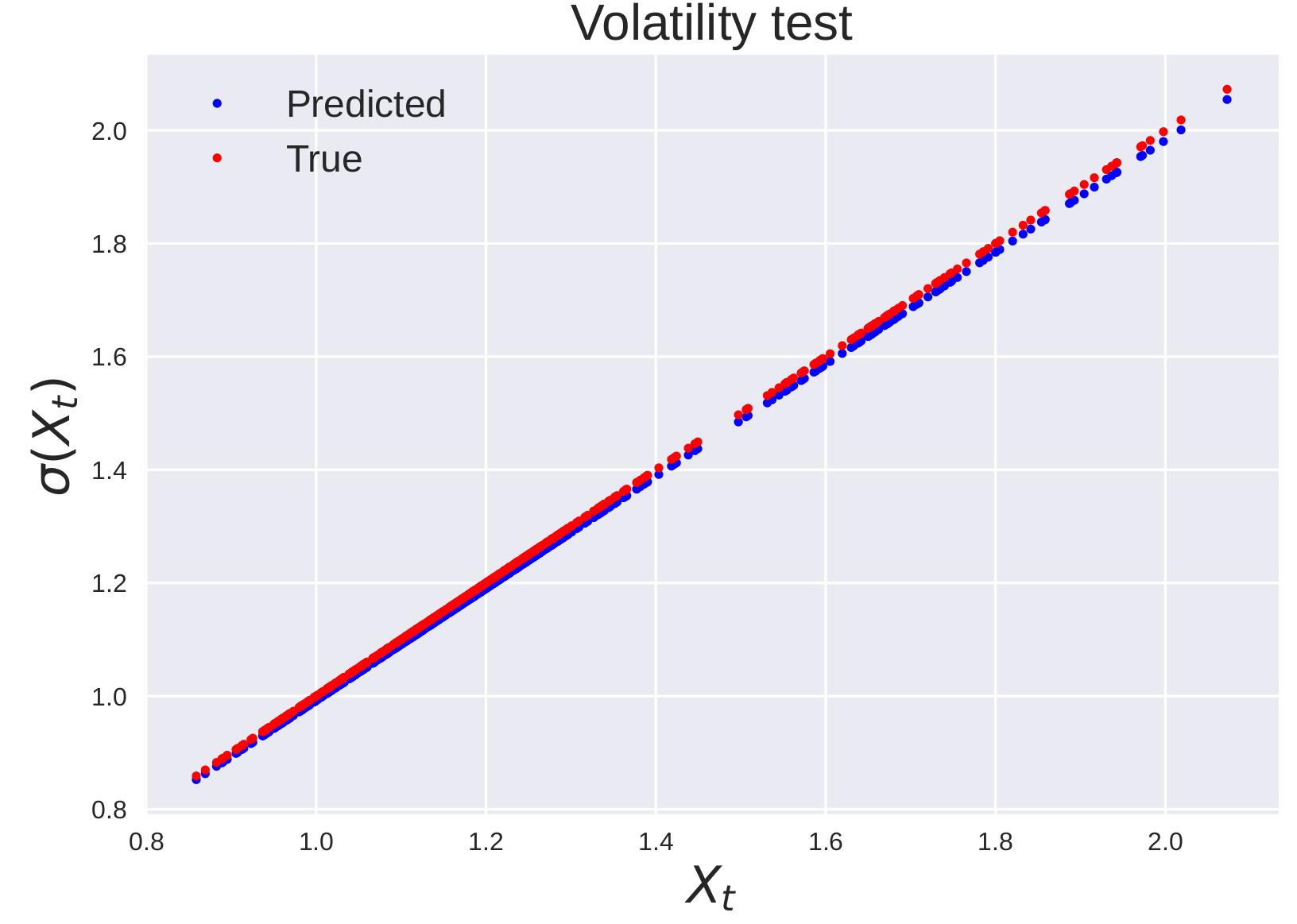
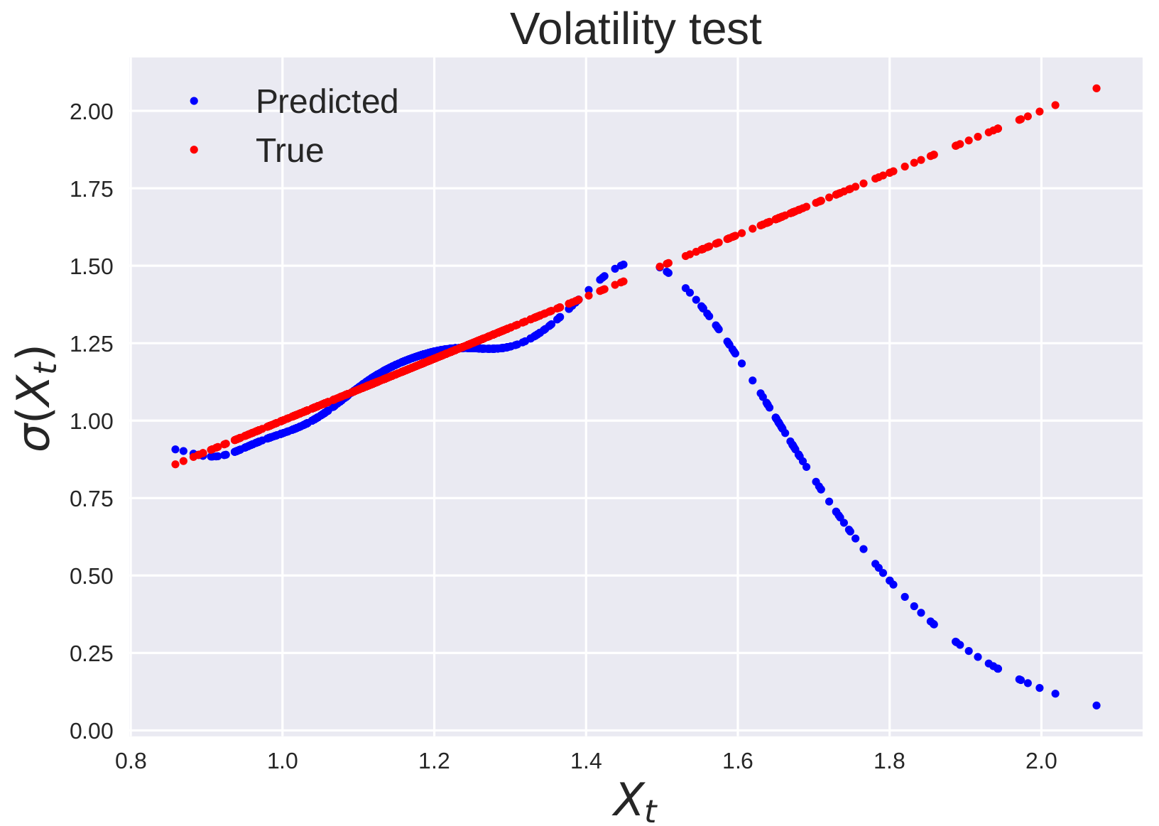
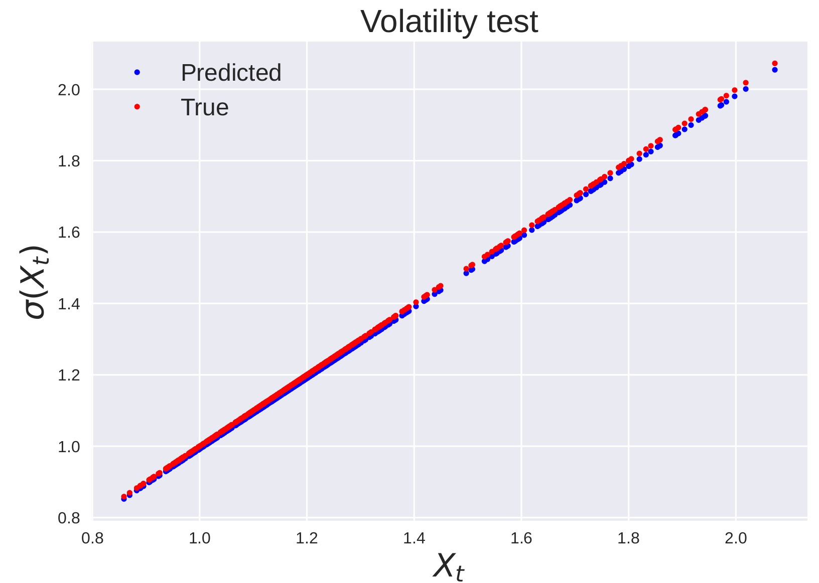
which has both non-stationary drift and diffusion functions. In section 6, we will show (see figure 1) how our hyper-parameter learning algorithm enables a non-perfectly-adapted kernel (e.g., a Matérn kernel for approximating the drift and volatility of (13)) to perform comparably to a perfectly adapted kernel (e.g., a linear kernel for approximating the drift and volatility of (13)). We also note that learning the kernel improves out-of-sample predictions.

Figure 1. Predicted volatility: well-specified kernel (left), ill specified kernel (middle), and well-specified kernel with learned parameters(right).

4.2. Methodology

We now describe how to select the kernels $K,G$ in a family of kernels parameterized by $\theta_{k},\theta_{g}$, which we learn from data using a cross-validation approach. Writing

$$\boldsymbol{\theta}:=(\theta_{k},\theta_{g})\,,$$ (14)

for the vector formed by all the hyperparameters of our approach, we learn $\theta$ through a robust-learning cross-validation approach which we will now describe. Consider the set of all sets of possible partitions of the training data $\mathcal{D}_{\mathcal{T}}$ with indices $\mathcal{I}$ into two mutually disjoint subsets of equal size.

$$\mathcal{A}=\{(\Pi,\Pi^{c})|\Pi\cup\Pi^{c}=\mathcal{I},\Pi\cap\Pi^{c}=\emptyset,|\Pi|=\frac{|\mathcal{I}|}{2}\}.$$ (15)

Write $\mathcal{D}_{\Pi}=(x_{j},y_{j})_{j\in\Pi}$ for the set of points belonging to the first partition and $\mathcal{D}_{\Pi^{c}}=(x_{j},y_{j})_{j\in\Pi^{c}}$ for the set of points belonging to the second set. Write $\mathbb{E}_{(\Pi,\Pi^{c})}$ for the uniform distribution over $\mathcal{A}$. For $(\Pi,\Pi^{c})\in\mathcal{A}$ write $\mathcal{L}(\mathcal{D}_{\Pi^{c}},\bar{f},\bar{\sigma})$ for the MAP loss (5) calculated with dataset $\mathcal{D}_{\Pi^{c}}$. Write

$$\begin{split}\mathcal{L}_{\text{CV}}(\boldsymbol{\theta};\bar{f}^{*},\bar{\sigma}^{*},\mathcal{D}_{\Pi})&=-\ln p(Y_{\Pi}|\bar{f}^{*},\bar{\sigma}^{*},X_{\Pi})\\ &=\sum_{i}\frac{(Y_{i}-\bar{f}^{*}_{i}\Delta t_{i})^{2}}{2(\bar{\sigma}_{i}^{*2}\Delta t_{i}+\lambda)}+\frac{1}{2}\ln(\bar{\sigma}_{i}^{*2}\Delta t_{i}+\lambda),\end{split}$$ (16)

for the negative log-likelihood of the validation data $\mathcal{D}_{\Pi}$ given $\bar{f}^{*},\bar{\sigma}^{*}$. Our proposed cross-validation approach is then to select $\boldsymbol{\theta}^{*}$ as

$$\begin{array}[]{ll}&\boldsymbol{\theta}^{*}=\underset{\boldsymbol{\theta}}{\arg\min}\,\,\mathbb{E}_{(\Pi,\Pi^{c})}\{\mathcal{L}_{\text{CV}}(\boldsymbol{\theta};\bar{f}^{*},\bar{\sigma}^{*},\mathcal{D}_{\Pi})\}\\ \mathrm{subject\,to}&\bar{f}^{*},\bar{\sigma}^{*}=\underset{\bar{f},\bar{\sigma}}{\arg\min}\,\,\mathcal{L}(\mathcal{D}_{\Pi^{c}},\bar{f},\bar{\sigma})\end{array}$$ (17)

Note that $\bar{f}^{*},\bar{\sigma}^{*}$ are selected as described in Section 3. In practice, the computation of the exact value of $\mathbb{E}_{(\Pi,\Pi^{c})}\{\mathcal{L}_{\text{CV}}(\boldsymbol{\theta};\bar{f}^{*},\bar{\sigma}^{*},\mathcal{D}_{\Pi}\}$ is intractable. Therefore, we instead approximate $\mathbb{E}_{(\Pi,\Pi^{c})}\{\mathcal{L}_{\text{CV}}\}$ with the empirical average

$$\frac{1}{M}\sum_{i=1}^{M}\mathcal{L}_{\text{CV}}(\boldsymbol{\theta};\bar{f}_{i}^{*},\bar{\sigma}_{i}^{*},\mathcal{D}_{\Pi_{i}})$$ (18)

where the $(\Pi_{i},\Pi_{i}^{c})$ are i.i.d. samples from $\mathbb{P}_{(\Pi,\Pi^{c})}$ and $\bar{f}_{i}^{*},\bar{\sigma}_{i}^{*}=\underset{\bar{f},\bar{\sigma}}{\arg\min}\,\,\mathcal{L}(\mathcal{D}_{\Pi_{i}^{c}},\bar{f},\bar{\sigma})$. We use a gradient free optimization algorithm to minimize (18) (see Subsection 4.3). This algorithm only uses noisy observations (18) of the true loss.

The proposed cross-validation algorithm can be summarized as follows:

1. Select a gradient-free optimization algorithm.

2. At each iteration, given the hyperparameters $\boldsymbol{\theta}^{k}$, select $M$ divisions of the data $\mathcal{D}_{\mathcal{T}}$ into a training set $\mathcal{D}_{\Pi_{i}^{c}}$ and a validation set $\mathcal{D}_{\Pi_{i}}$.

3. For each $1\leq i\leq M$, recover $\bar{f}^{*}_{i},\bar{\sigma}^{*}_{i}$ using training data $\mathcal{D}_{\Pi_{i}^{c}}$ using hyper-paramters $\boldsymbol{\theta}^{k}$.

4. For each $1\leq i\leq M$, compute the loss $\mathcal{L}(\boldsymbol{\theta}^{k};\bar{f}_{i}^{*},\bar{\sigma}_{i}^{*},\mathcal{D}_{\Pi_{i}})$ and the empirical average (18).

5. Minimize (18) with the gradient free optimization algorithm to select $\boldsymbol{\theta}^{k+1}$.

4.3. The active learning algorithm

We choose the Bayesian optimization algorithm [54], where the loss function is modeled using a Gaussian Process with Matern kernel [50], implemented in the scikit-optimize library in Python [1]. In our case, we set $M=1$ when using gradient descent minimization and $M=10$ when using Newton’s method for minimization. The maximum number of iterations for the Bayesian optimization algorithm is set to $K=75$ when using gradient descent minimization and $K=150$ when using Newton’s method for minimization. While we can use a greater number of samples and a greater number of iterations with Newton’s method because of its greater speed, in practice, the gradient descent method offered better performance in our tests.

5. Experimental results

We first illustrate the effectiveness of our methods by considering two systems with non-linear drift or volatility. The two processes we consider are:

$$dX_{t} =\mu X_{t}dt+b\exp(-X_{t}^{2})dW_{t}$$ Exponential decay volatility. (19)

$$dX_{t} =\sin(2k\pi X_{t})dt+b\cos(2k\pi X_{t})dW_{t}$$ Trigonometric process. (20)

In both cases, we generate trajectories using a Euler-Maruyama disretization. We use 500 points for training and 500 points for testing.

5.1. Metrics.

To measure the performance of each method, we use three metrics. The first is the likelihood of the model given the data of the test set defined as

$$\mathcal{L}(\bar{f}^{*},\bar{\sigma}^{*}|X,Y)=-\log(p(Y|\bar{f}^{*},\bar{\sigma}^{*},X))\propto\sum_{i=1}^{M}\frac{(Y_{i}-\bar{f}^{*}\Delta t_{i})^{2}}{2(\bar{\sigma}_{i}^{*2}\Delta t_{i}+\lambda)}+\frac{1}{2}\ln(\bar{\sigma}_{i}^{*2}\Delta t_{i}+\lambda).$$

The other two metrics are the relative error of the test drift and volatility at the test points:

$$\delta_{f}=\frac{||f-\bar{f}||}{||f||}$$

$$\delta_{\sigma}=\frac{||\sigma-\bar{\sigma}||}{||\sigma||}$$

where $f$ is the vector of drift values at the test points $(f)_{i}=f(X_{i})$ and $\bar{f}$ is the vector of prediction $(\bar{f})_{i}=\bar{f}(X_{i})$ (likewise for $\sigma,\bar{\sigma}$). Note that in practice, only $\mathcal{L}(\bar{f}^{*},\bar{\sigma}^{*}|(X,Y))$ may be computed without access to the true drift $f$ and true volatility $\sigma$. We still compute $\delta_{f},\delta_{\sigma}$ to illustrate how a lower loss on the recovery of the drift and volatility yields a lower loss on the likelihood.

5.2. Choice of kernels

In all experiments, we use the Matérn Kernel [50] with smoothness parameter $\nu=\frac{5}{2}$ defined as

$$K_{\text{Mat\'{e}rn}}(x,y)=\sigma^{2}\Big{(}1+\frac{\sqrt{5}||x-y||}{l}+\frac{5||x-y||^{2}}{3l^{2}}\Big{)}\exp\Big{(}-\frac{\sqrt{5}||x-y||}{l}\Big{)}.$$ (21)

We learn the parameters $(\sigma,l)$ of the kernel (the smoothness parameter $\nu$ is not learned). Note that the Matérn kernel is not well specified for many of the processes we will consider as the processes it defines are only 3 times differentiable (in the mean square sense [50]) and hence it is overly general. A better specified of kernel can in many cases significantly improve the performance. We choose this kernel because it is very general and allows to illustrate how one can obtain good results with few assumptions and little domain knowledge.

5.3. Benchmarks.

We compare our method and optimized parameters with two baselines. A first baseline that uses our method and unoptimized parameters. For kernels using a lengthscale (such as the Matérn kernel (21)), it is set to be the average $\ell^{2}$ distance between data points:

$$l_{\text{unopt}}=\frac{1}{N(N-1)}\sum_{i\neq j}\left\lVert X_{i}-X_{j}\right\rVert.$$

All other paramters are set to $1.0$. This method is labeled as non-learned kernel.

The second baseline does not use our method to recover the drift and diffusion separately. Instead we assume that $Y$ is the sum of two Gaussian processes:

$$y(x)=\xi(x)+W(x)$$ (22)

where $\xi$ is a smooth Gaussian process (such as a Gaussian process with Matérn covariance function) and $W$ is a white noise Gaussian process with covariance matrix

$$K_{\text{wn}}(x_{i},x_{j})=c\delta(x_{i}-x_{j}).$$ (23)

The posterior distribution $y$ conditioned on the data provides a prediction for the conditional mean (the drift of the SDE) and the conditional variance (the volatility of the SDE).The parameters of the kernel are optimized through the minimization of the negative log marginal likelihood. This method is labeled as benchmark and uses the implementation present in [49] and the details are presented in Appendices B and C. Note that a major drawback of this method is the assumption that the noise $\sigma(X_{t})$ is identically distributed Gaussian noise, modeled through the white noise kernel $\delta(x_{i}-x_{j})$. This assumption is valid for only a restricted class of SDEs.

5.4. Exponential decay volatility.

The discretization of the exponential decay volatility is given by

$$X_{n+1}-X_{n}=\mu X_{n}\Delta t+b\exp(-X_{n}^{2})\sqrt{\Delta t}\xi_{n},\quad X_{0}=x_{0},$$ (24)

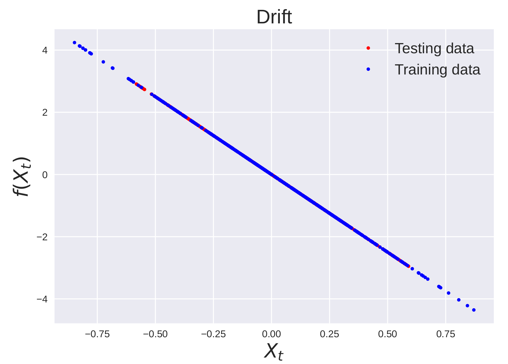
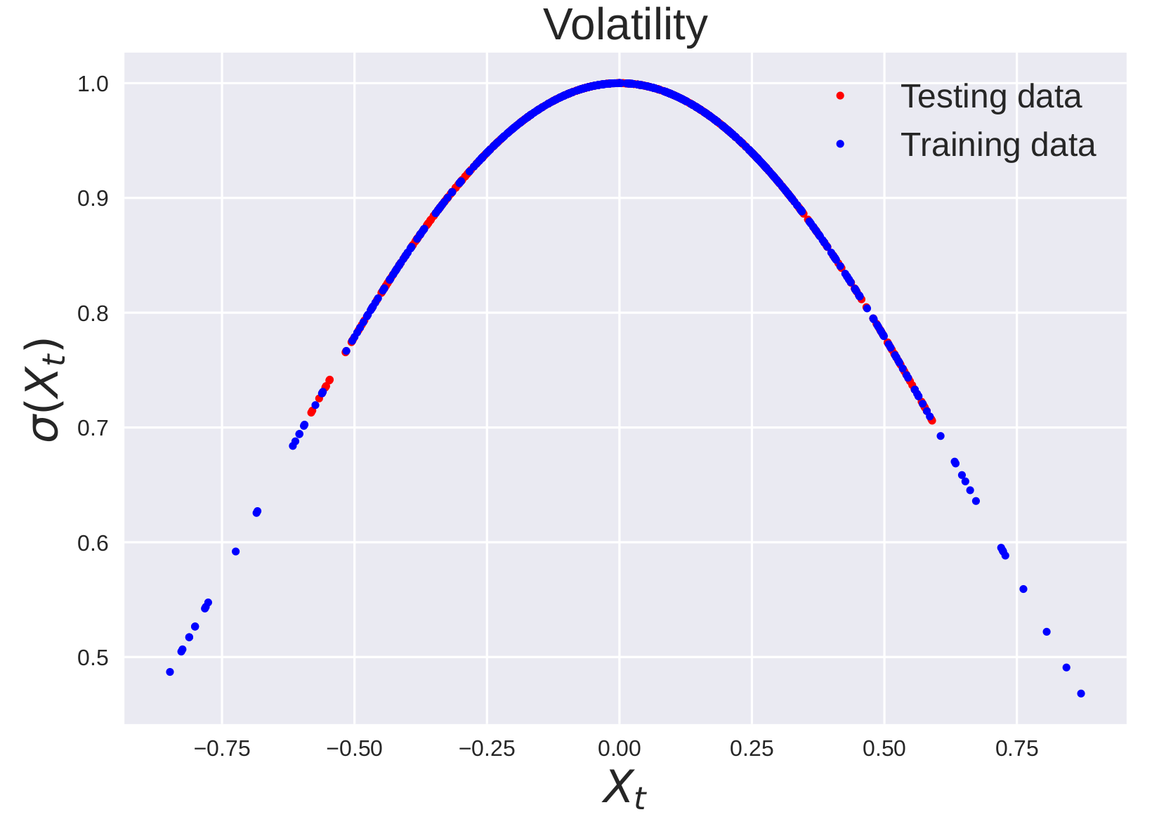
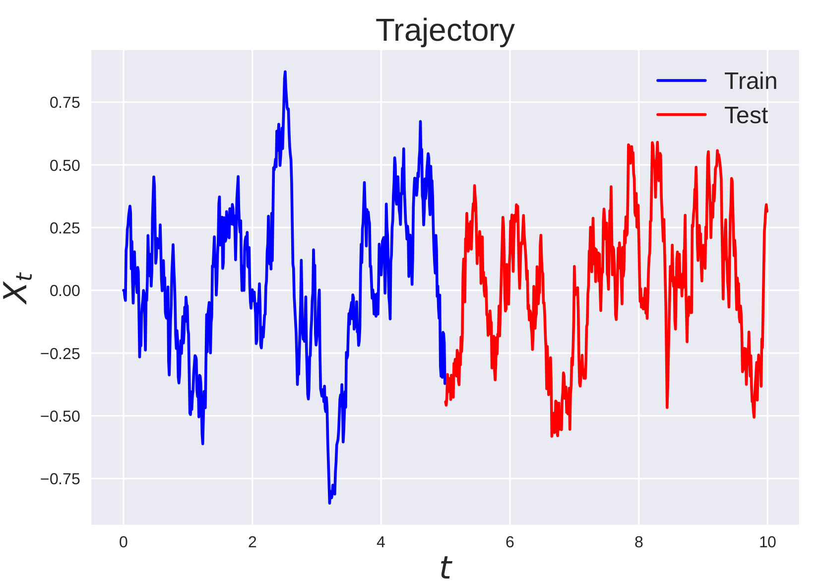
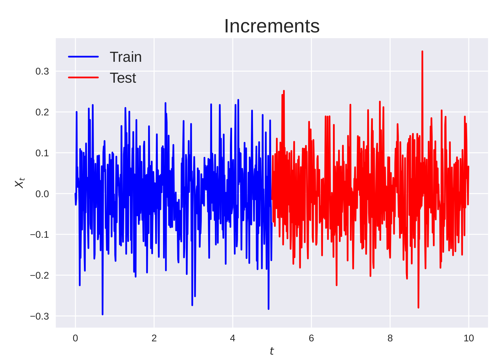
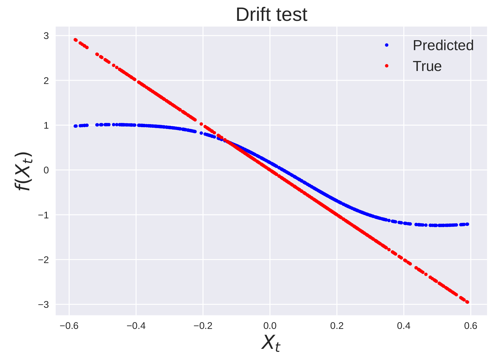
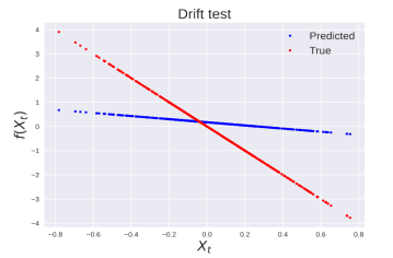
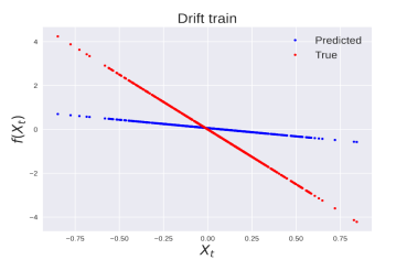
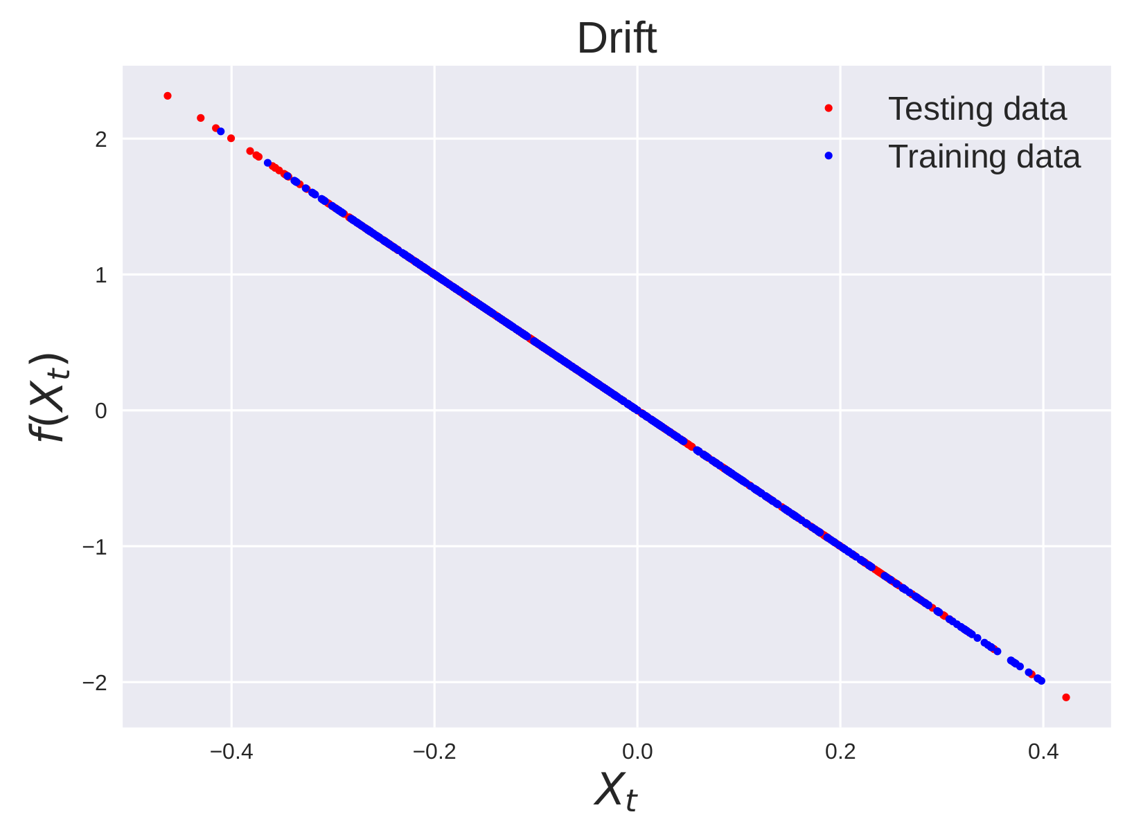
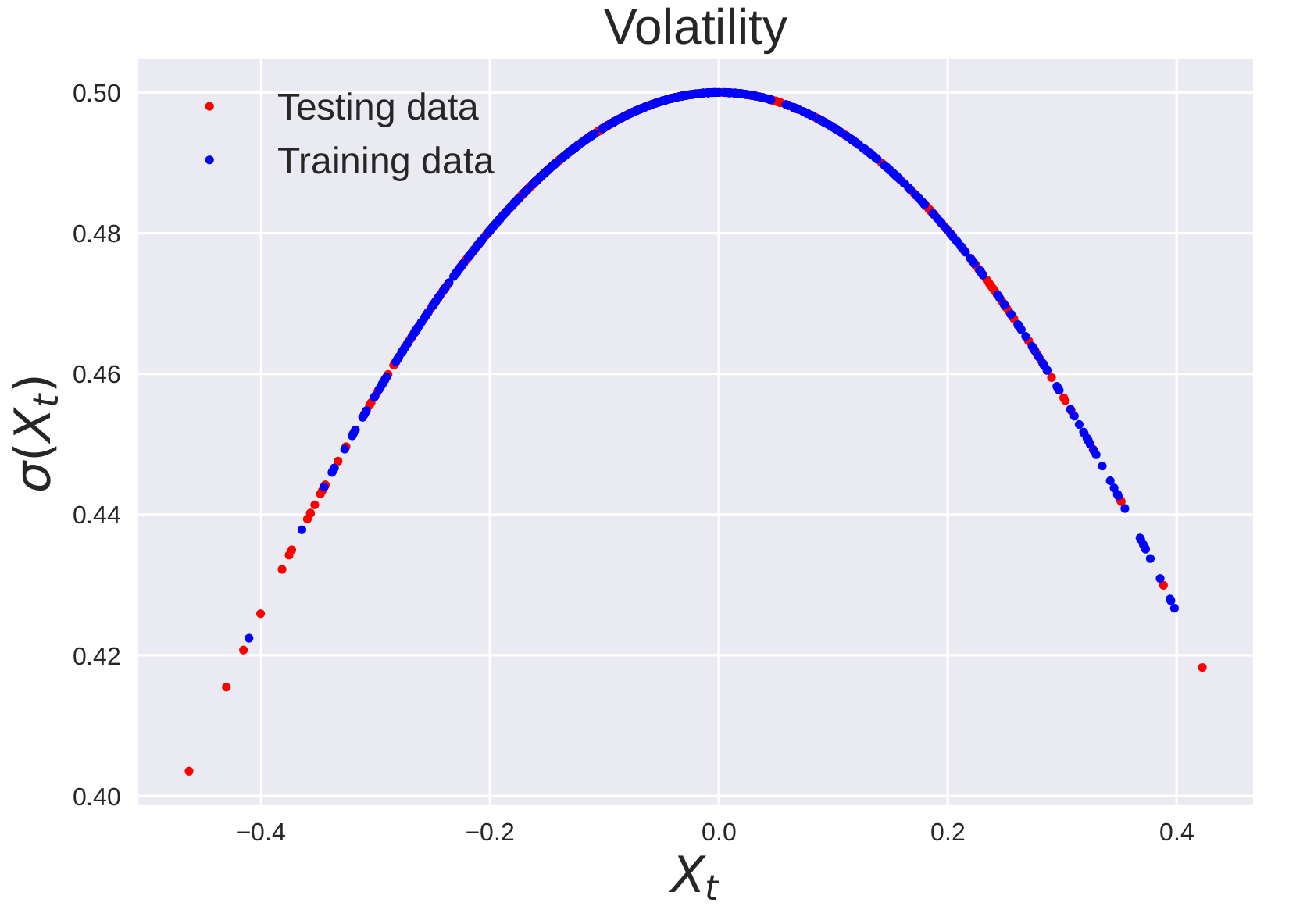
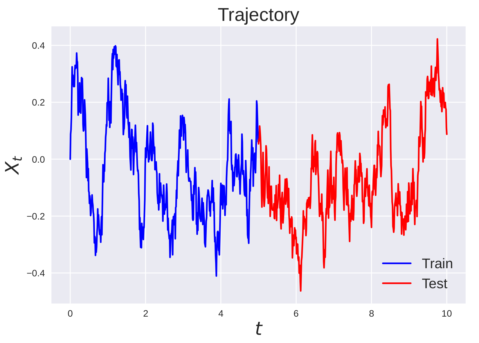
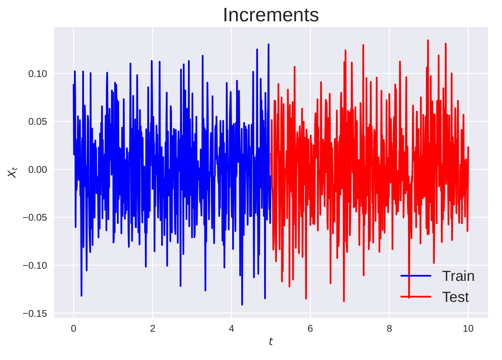
with timestep $\Delta t=0.01$. Observe that this process is pushed towards the origin by its drift value, where the volatility is maximized. Moreover, the volatility decreases exponentially fast away from the origin. We generate two trajectories with the same drift parameter $\mu=5$ and different volatility parameter $b=0.5,1.0$. The results for the learned and unlearned kernel are reported in table 1. The training and testing data are illustrated in figure 2 and the prediction of the drift and volatility are presented in figure 3 (see also figures 18, 19 in the appendix).

	Trajectory 1			Trajectory 2
	$\mathcal{L}(\bar{f}^{*},\bar{\sigma}^{*}|X,Y)$	$\delta_{f}$	$\delta_{\sigma}$	$\mathcal{L}(\bar{f}^{*},\bar{\sigma}^{*}|X,Y)$	$\delta_{f}$	$\delta_{\sigma}$
Benchmark	-2.547	0.394	0.033	-1.887	0.322	0.085
Non-learned kernel	-2.532	0.506	0.081	-1.887	0.472	0.062
Learned kernel	-2.546	0.388	0.048	-1.900	0.249	0.035

Table 1. Results for the exponential volatility process.

Figure 2. From left to right: drift function, volatility function, sample trajectory and sample increments of the exponential volatility process.

Figure 3. Predicted drift and volatility on the testing set for trajectory 2 of the exponential volatility process. From left to right: drift (non-learned kernel), volatility (non-learned kernel), drift (learned kernel), volatility (learned kernel) .

5.5. Trigonometric process

The discretization of the trigonometric process is given by

$$X_{n+1}-X_{n}=\sin(2k\pi X_{t})\Delta t+b\cos(2k\pi X_{t})\sqrt{\Delta t}\xi_{n},\quad X_{0}=x_{0}.$$ (25)

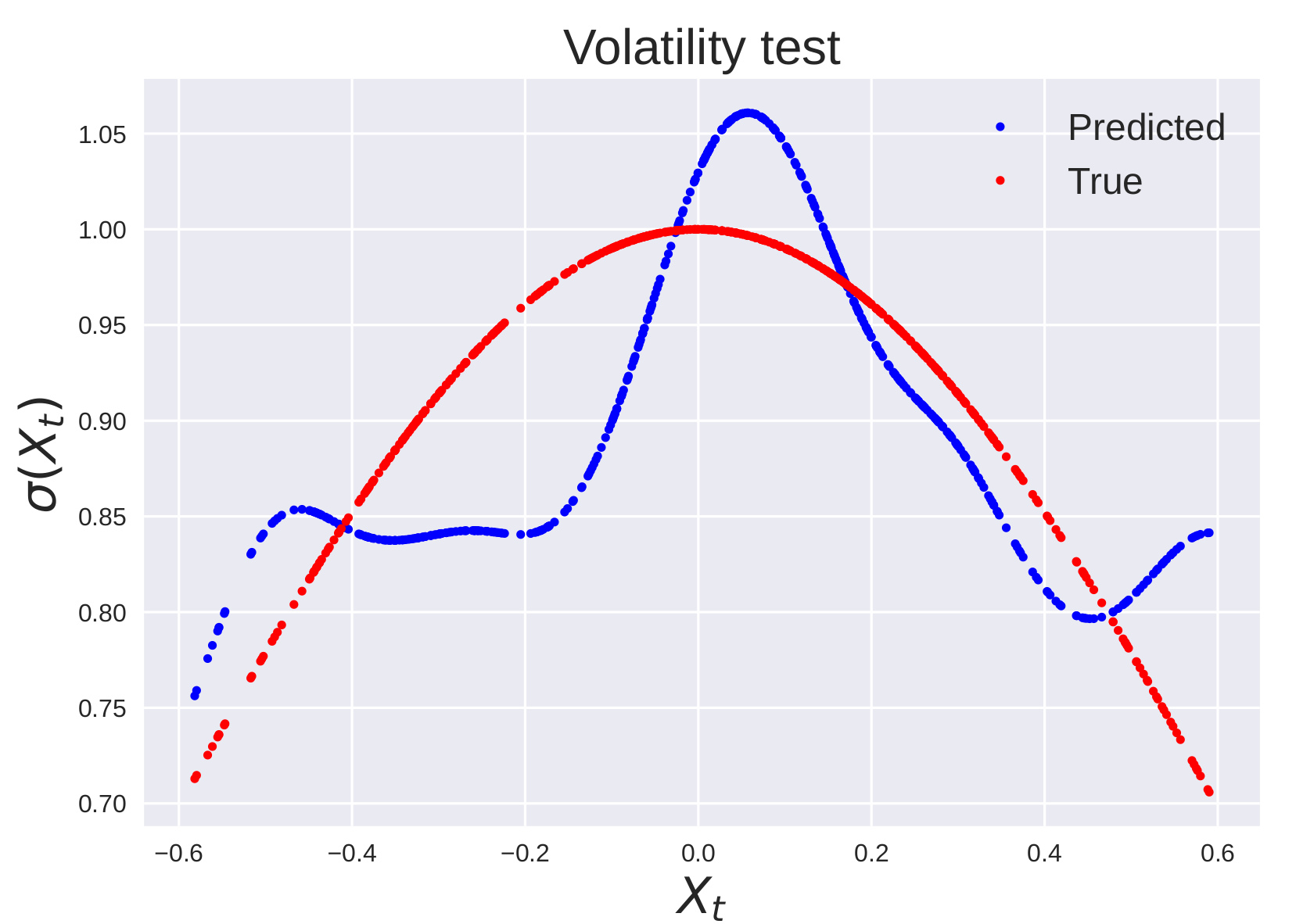
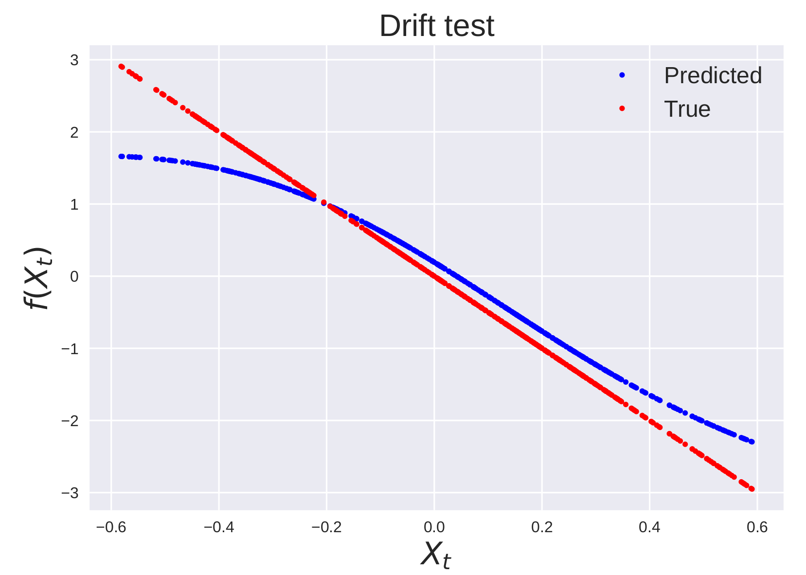
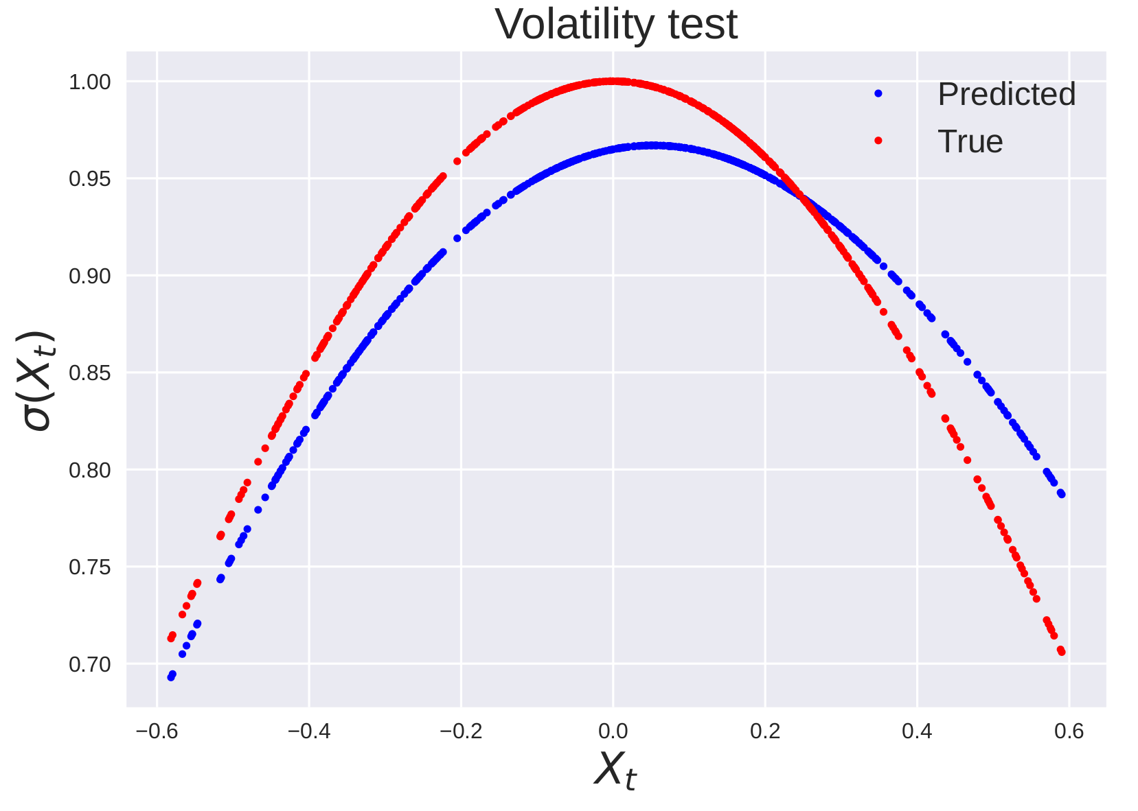
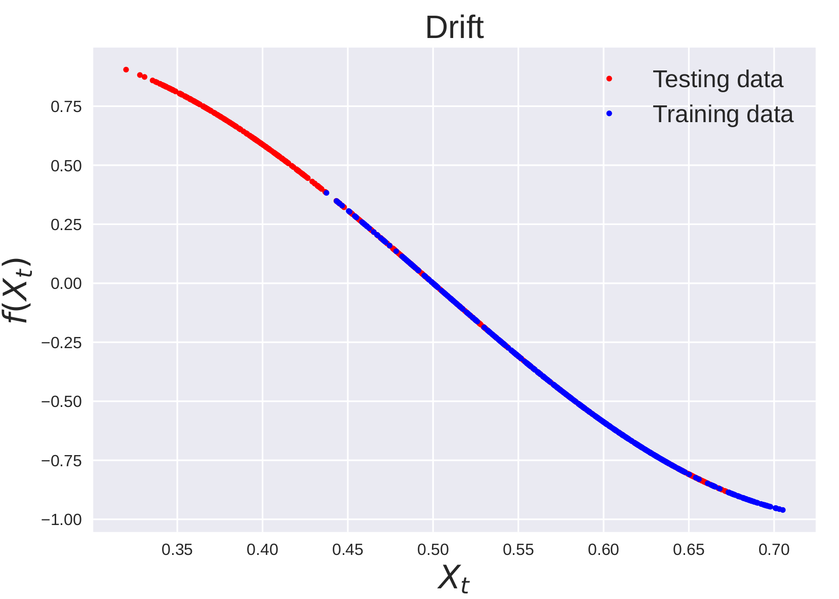
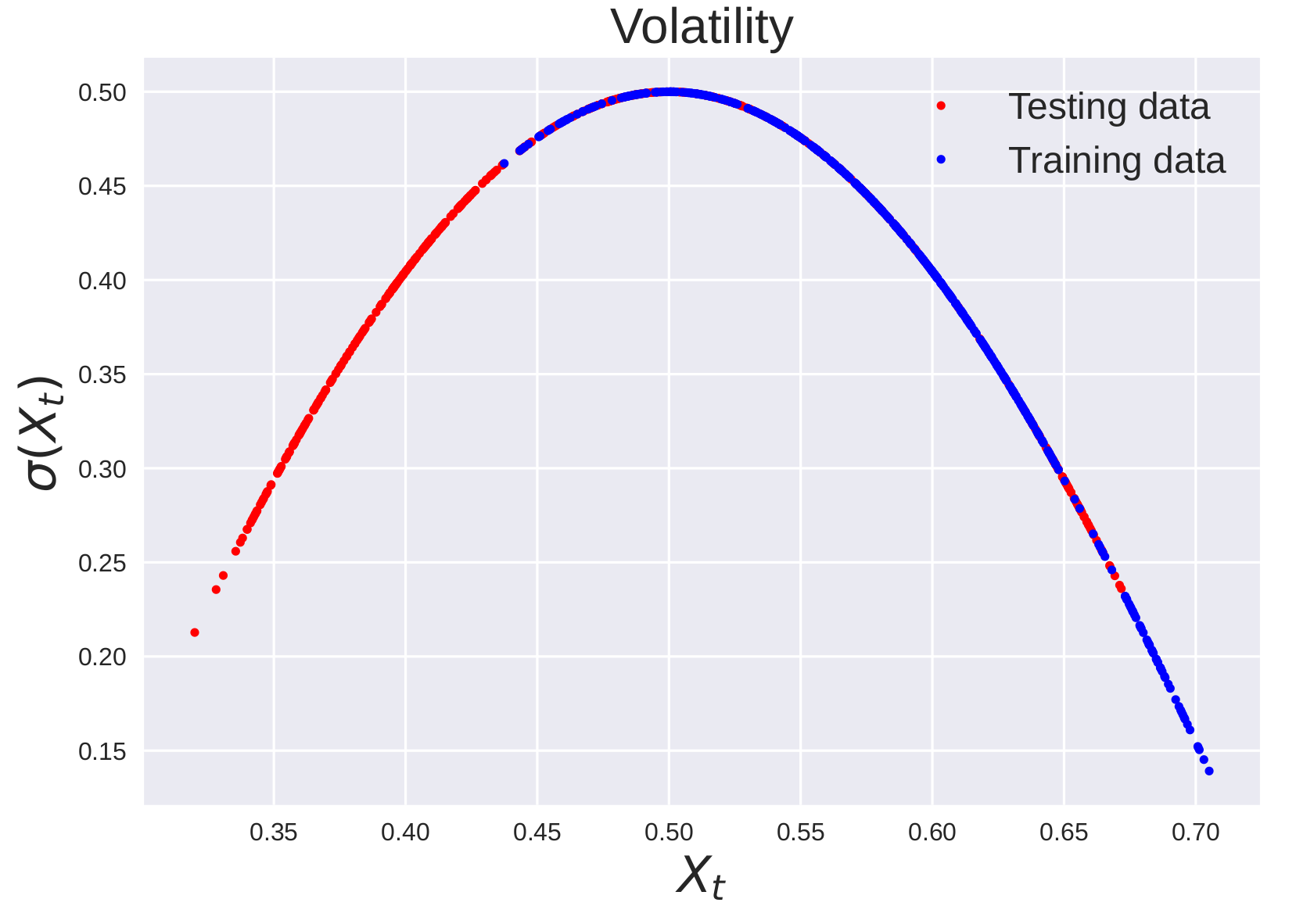
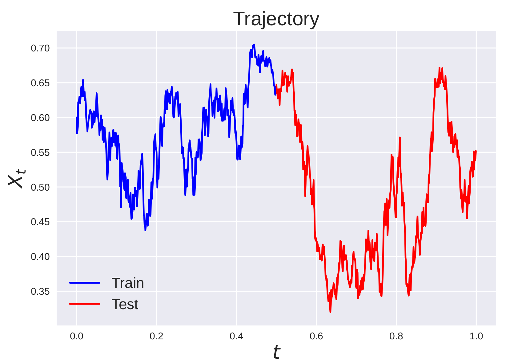
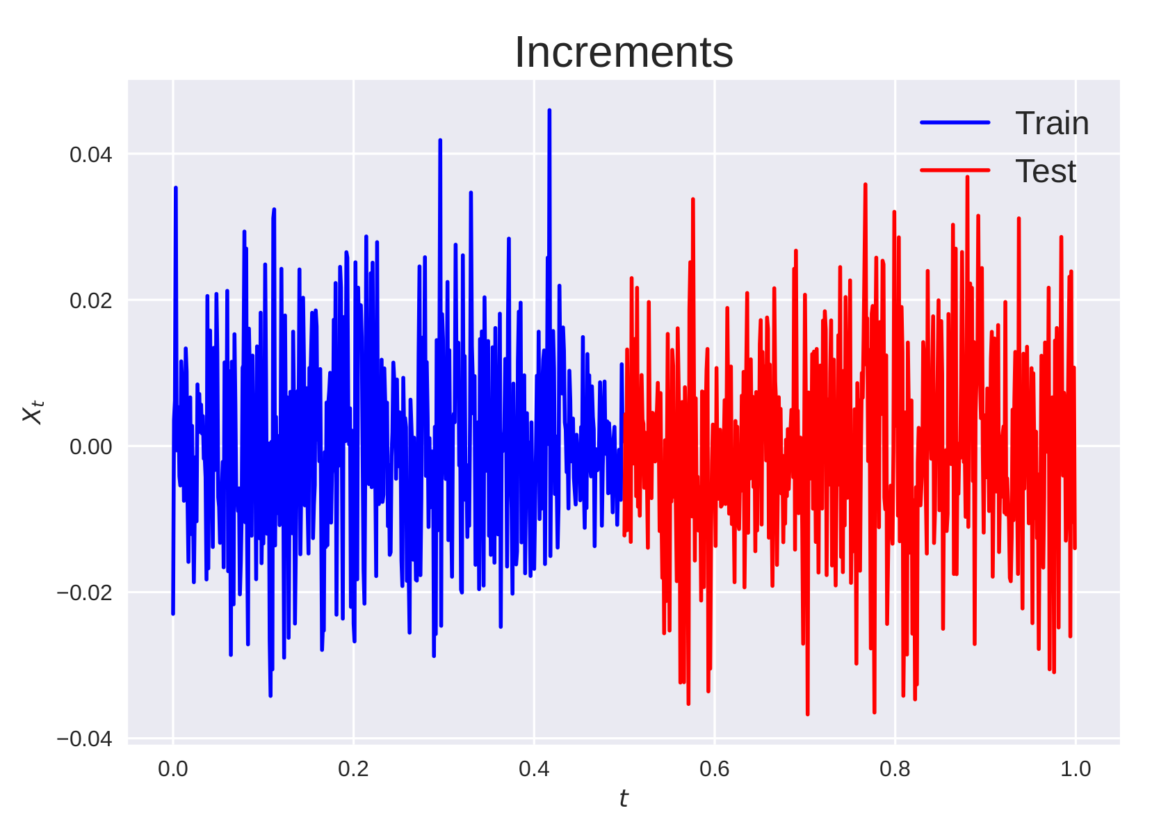
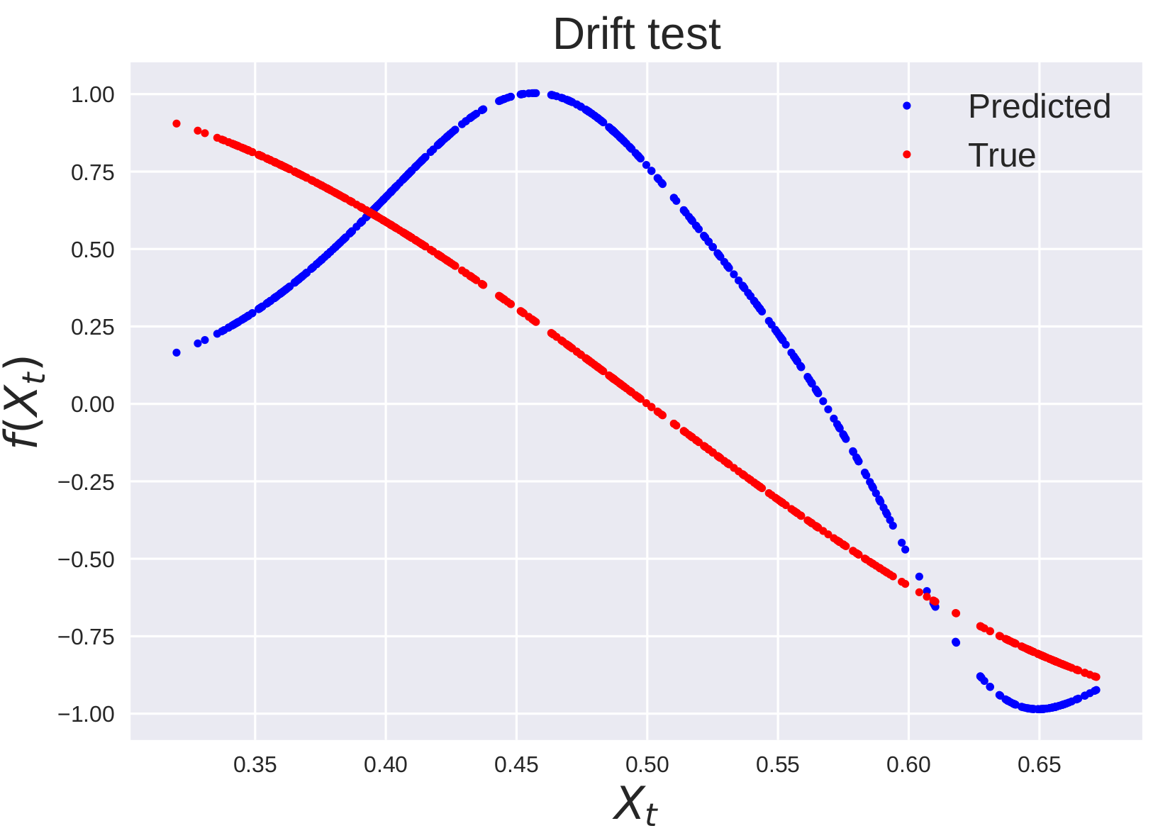
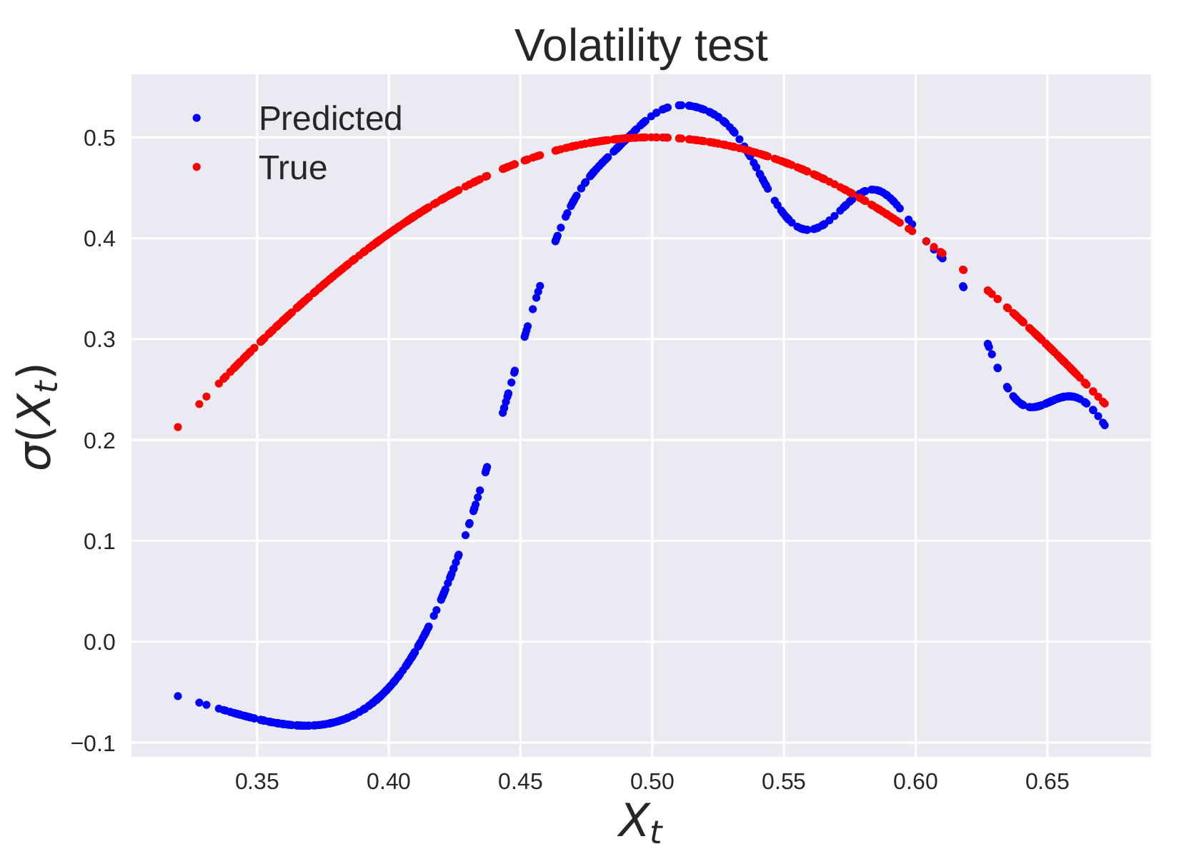
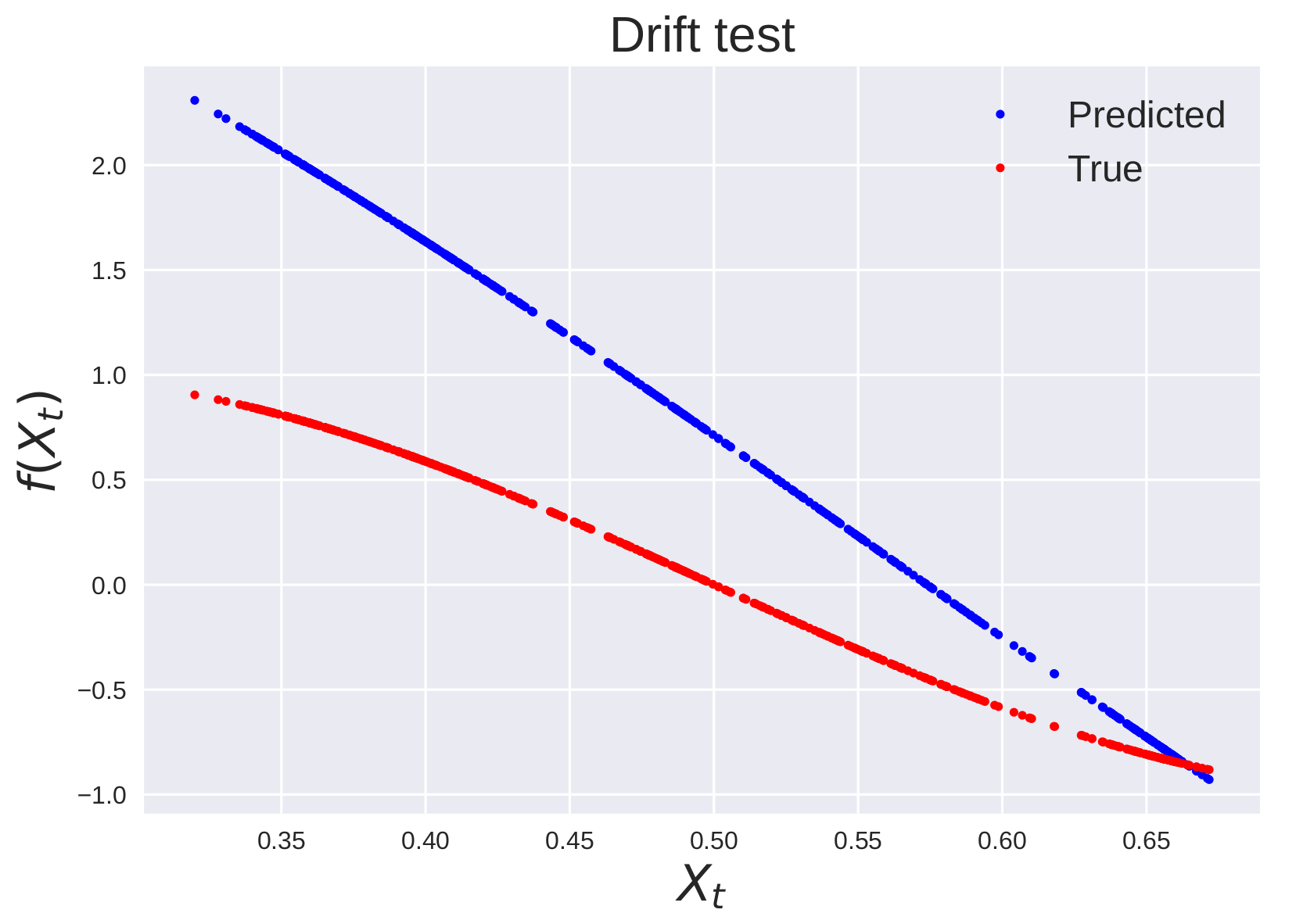
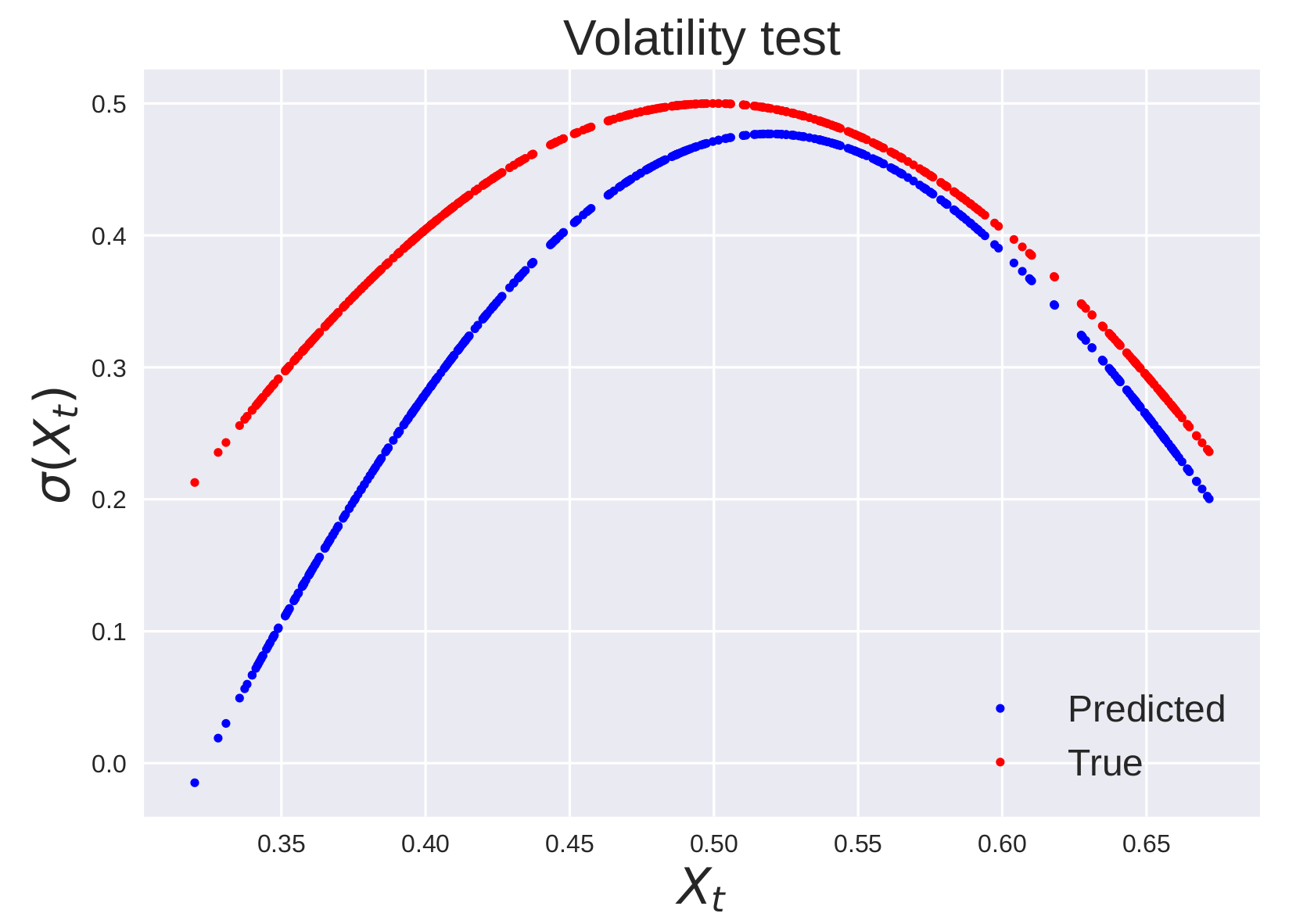
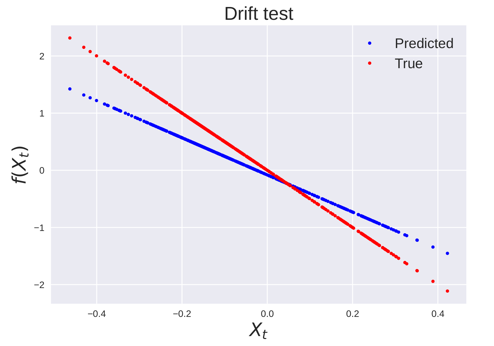
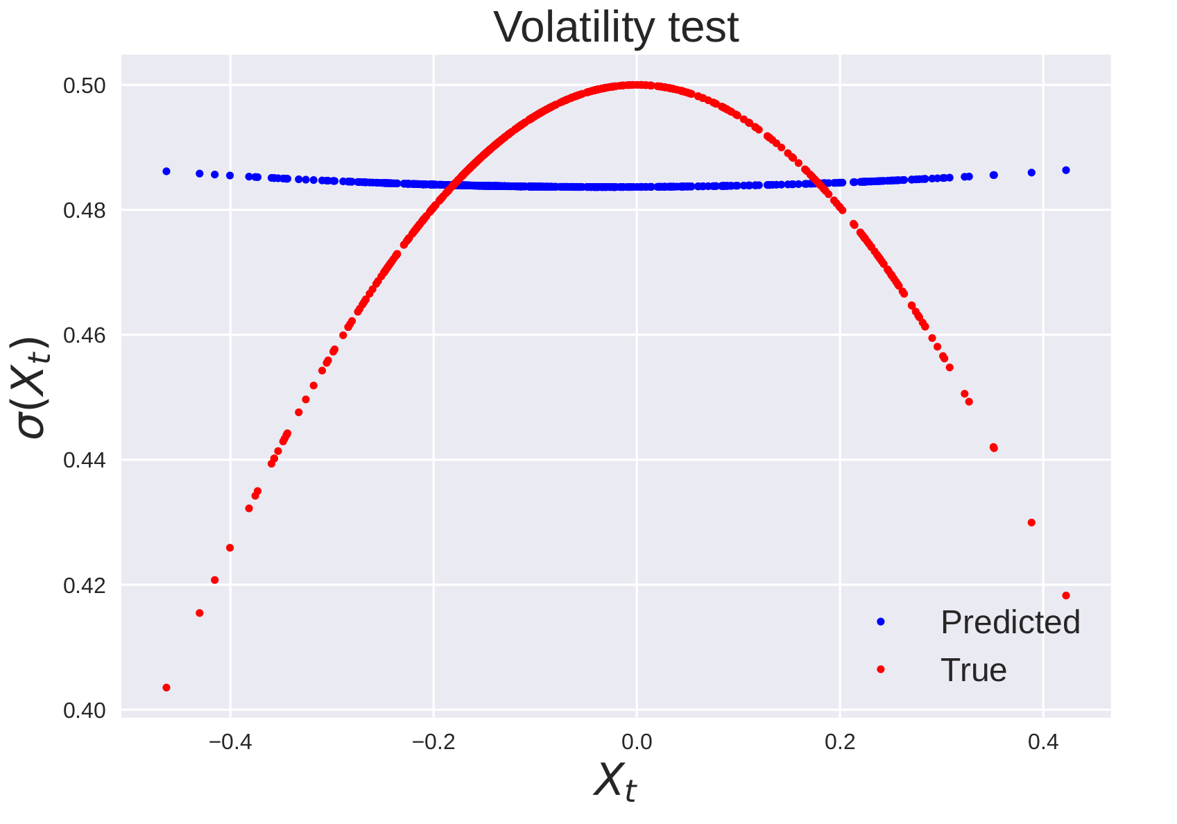
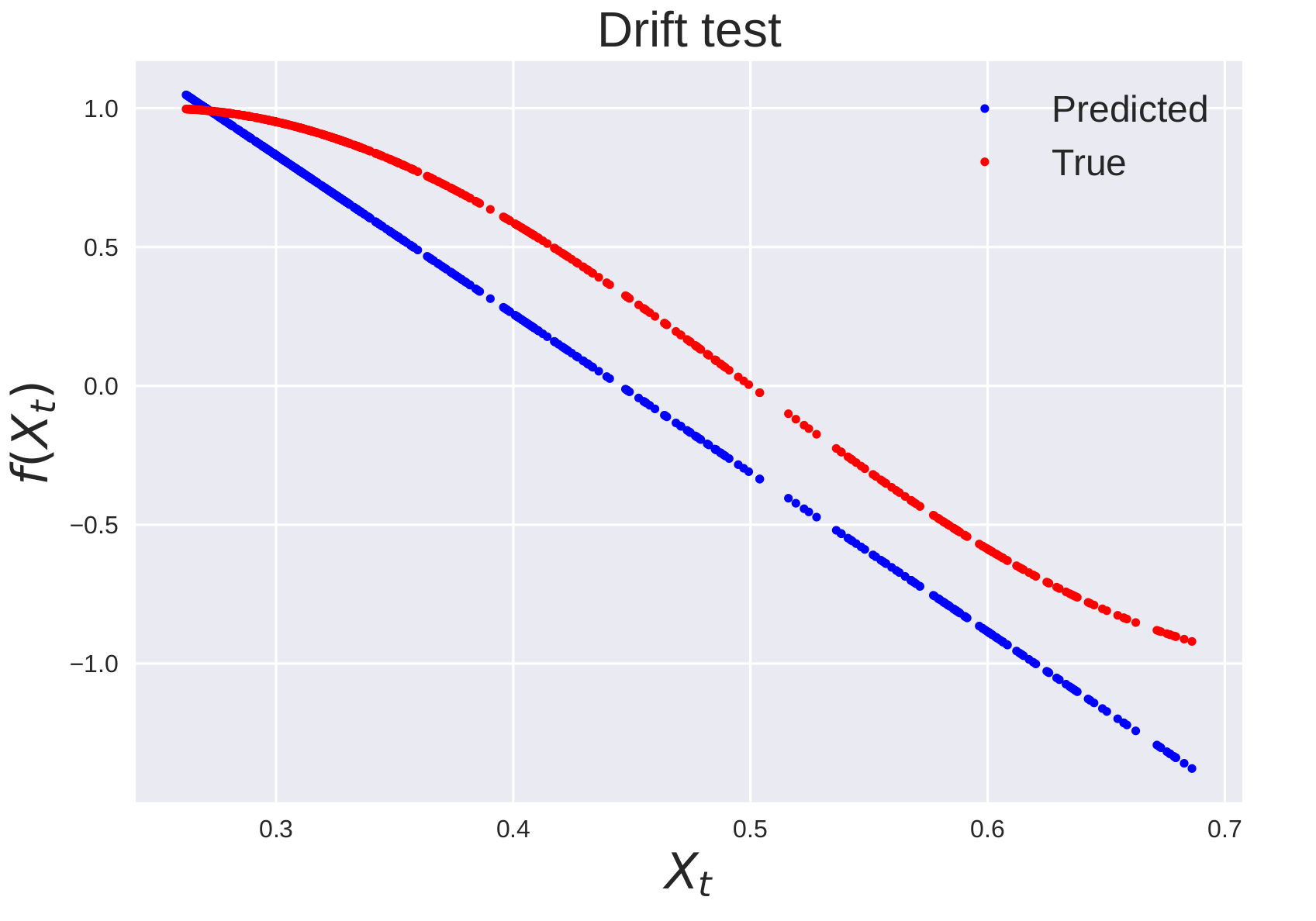
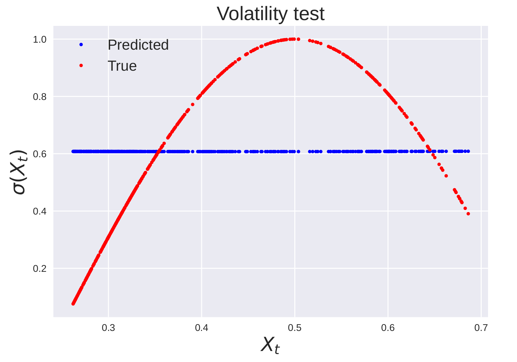
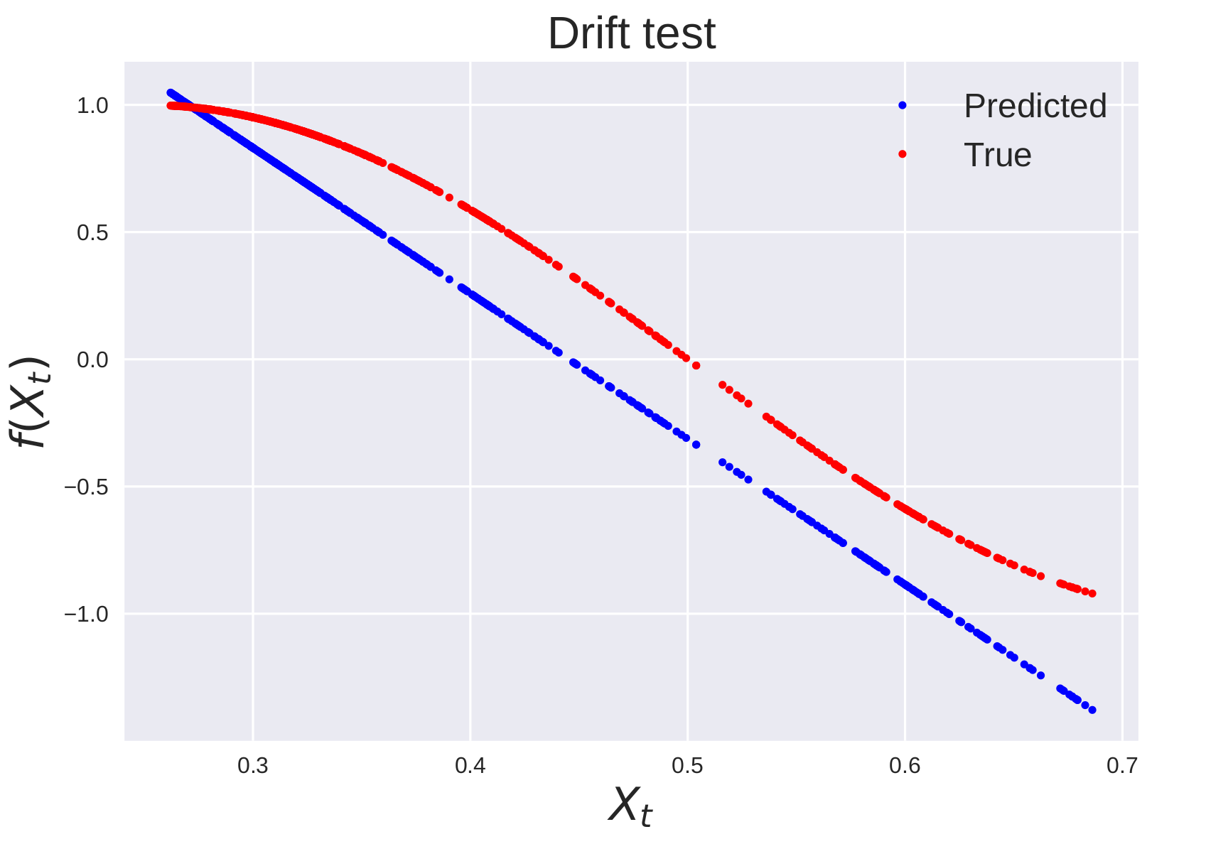
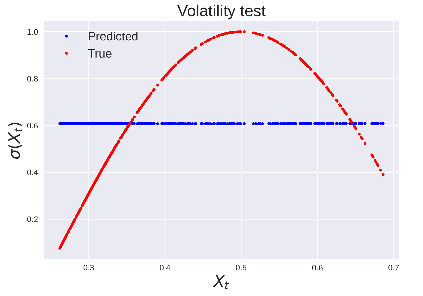
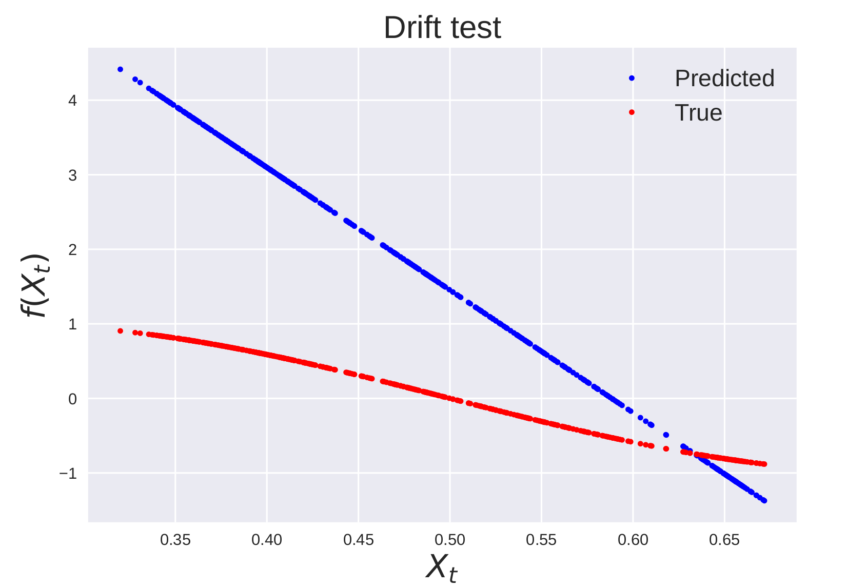
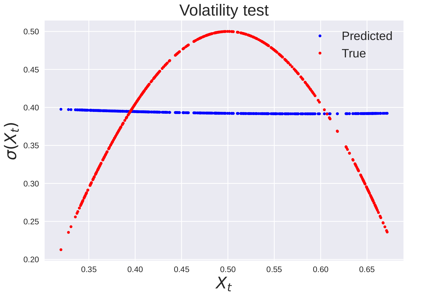
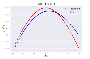
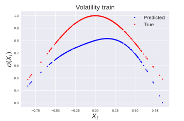
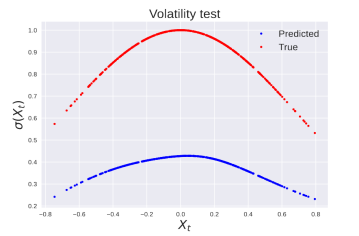
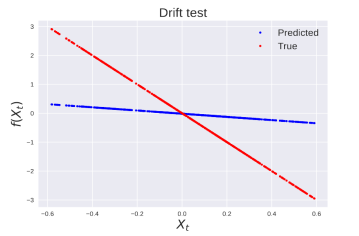
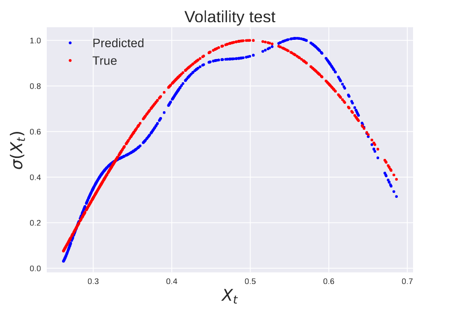
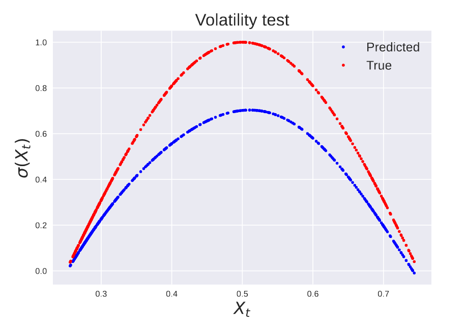
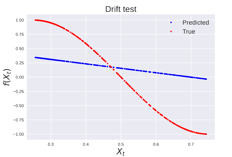
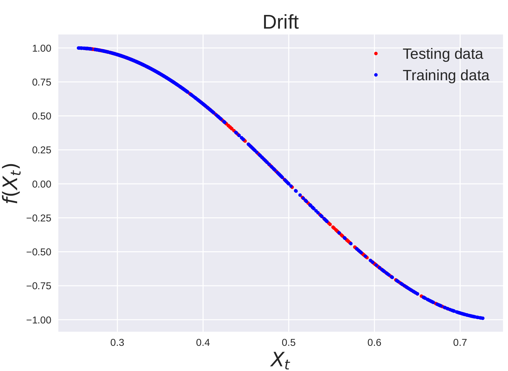
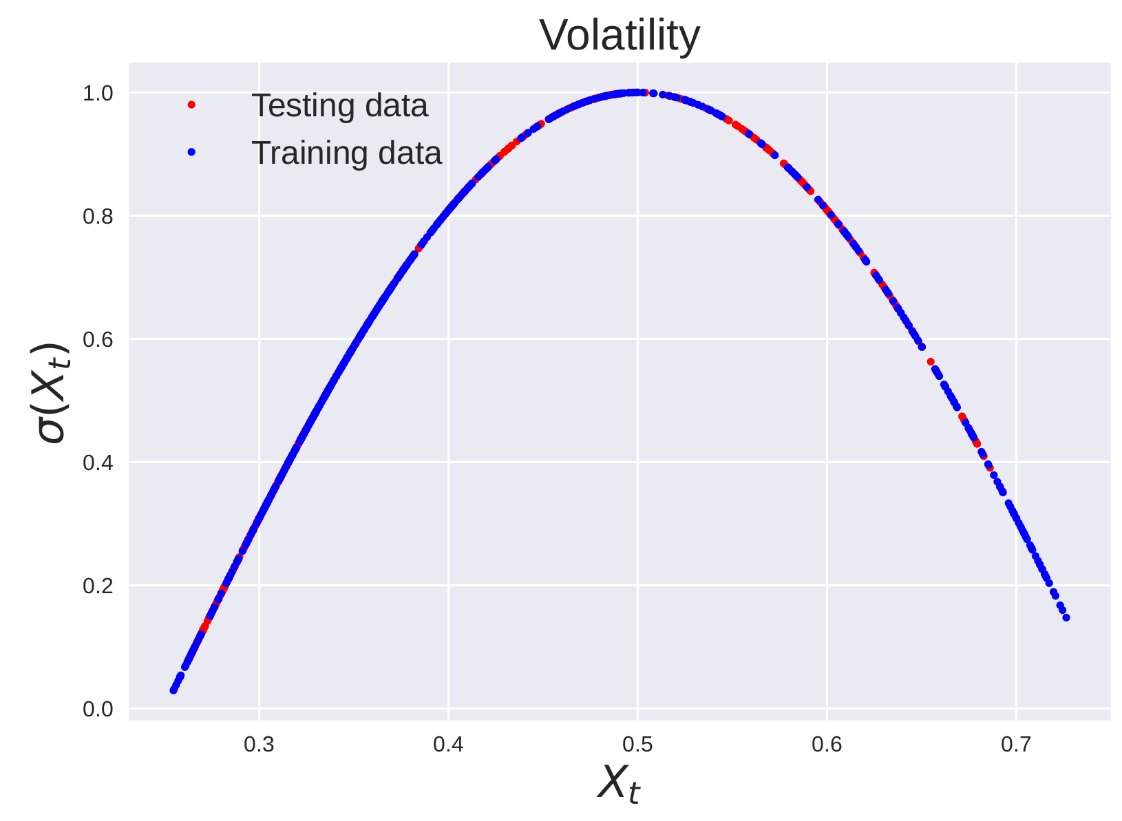
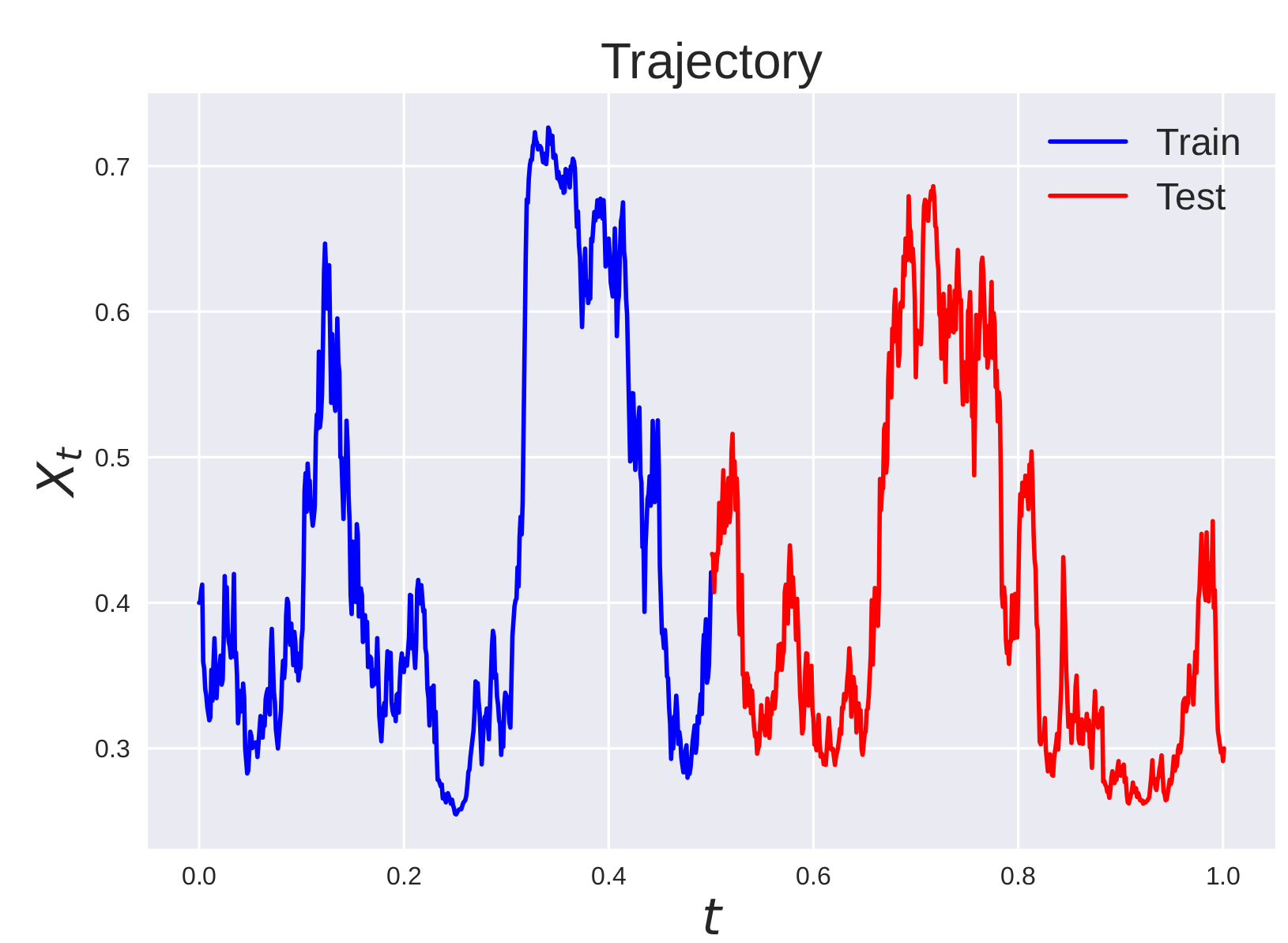
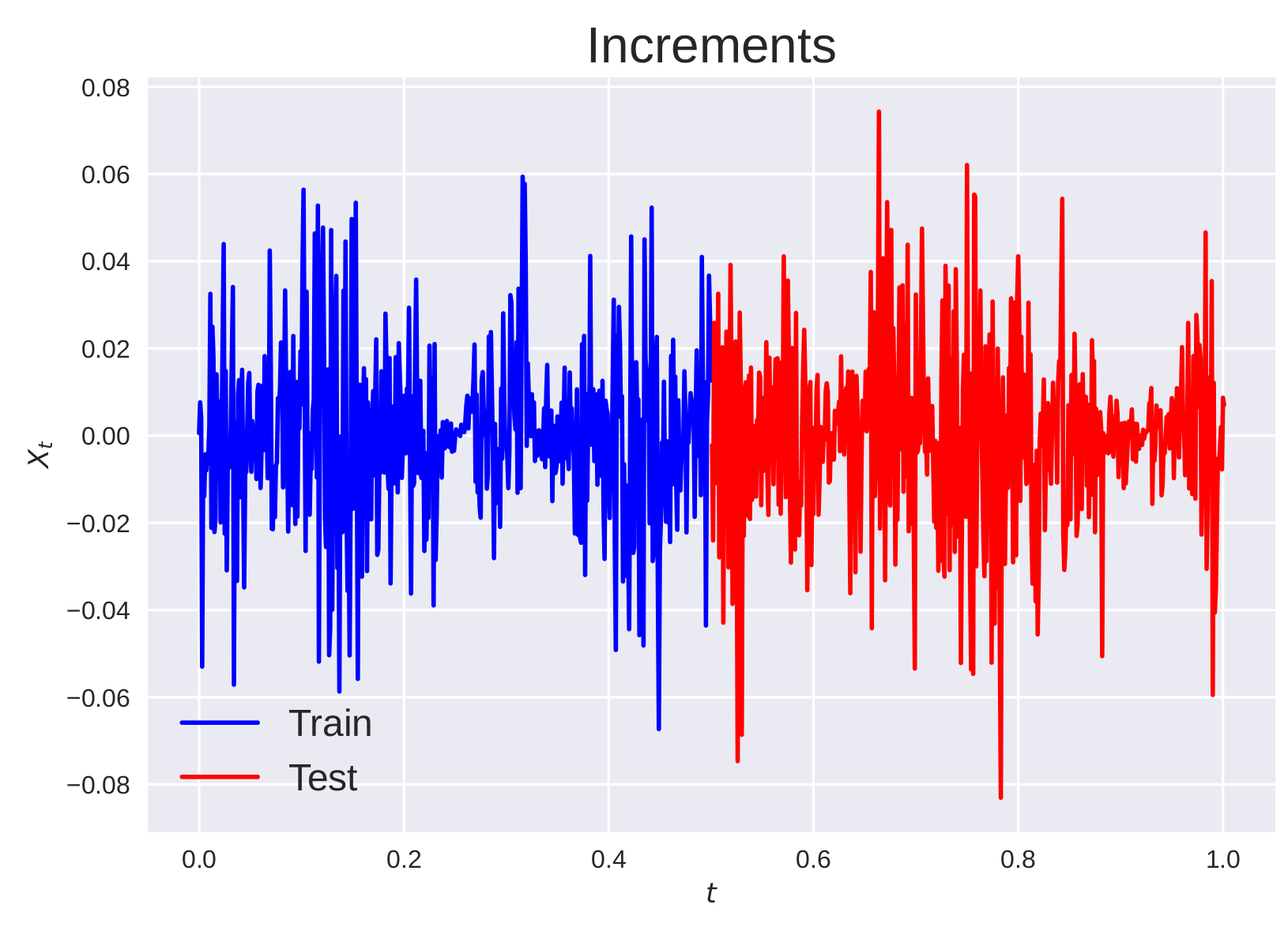
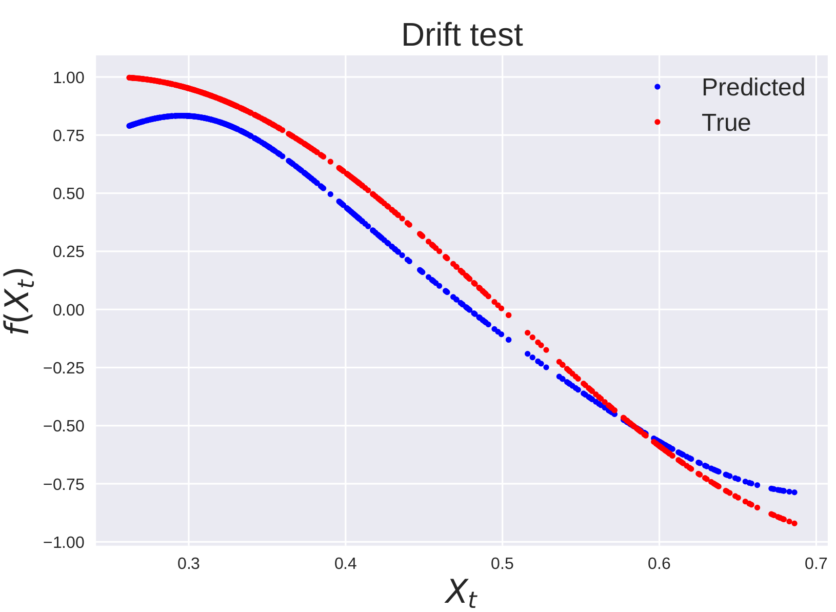
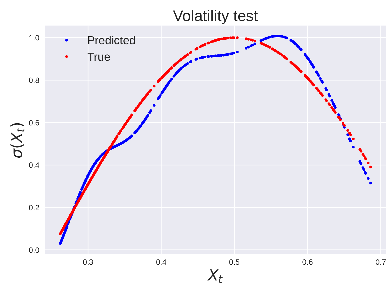
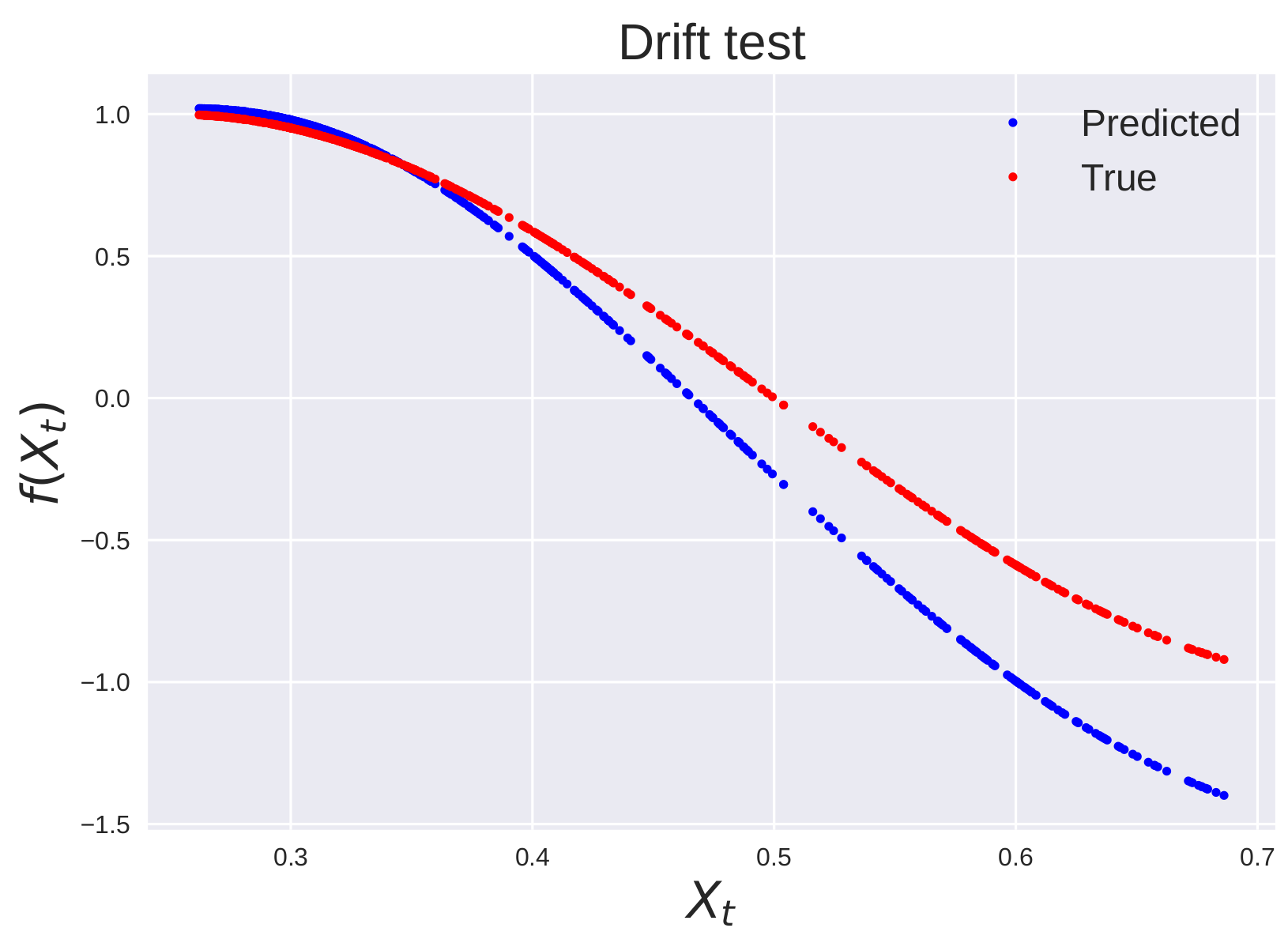
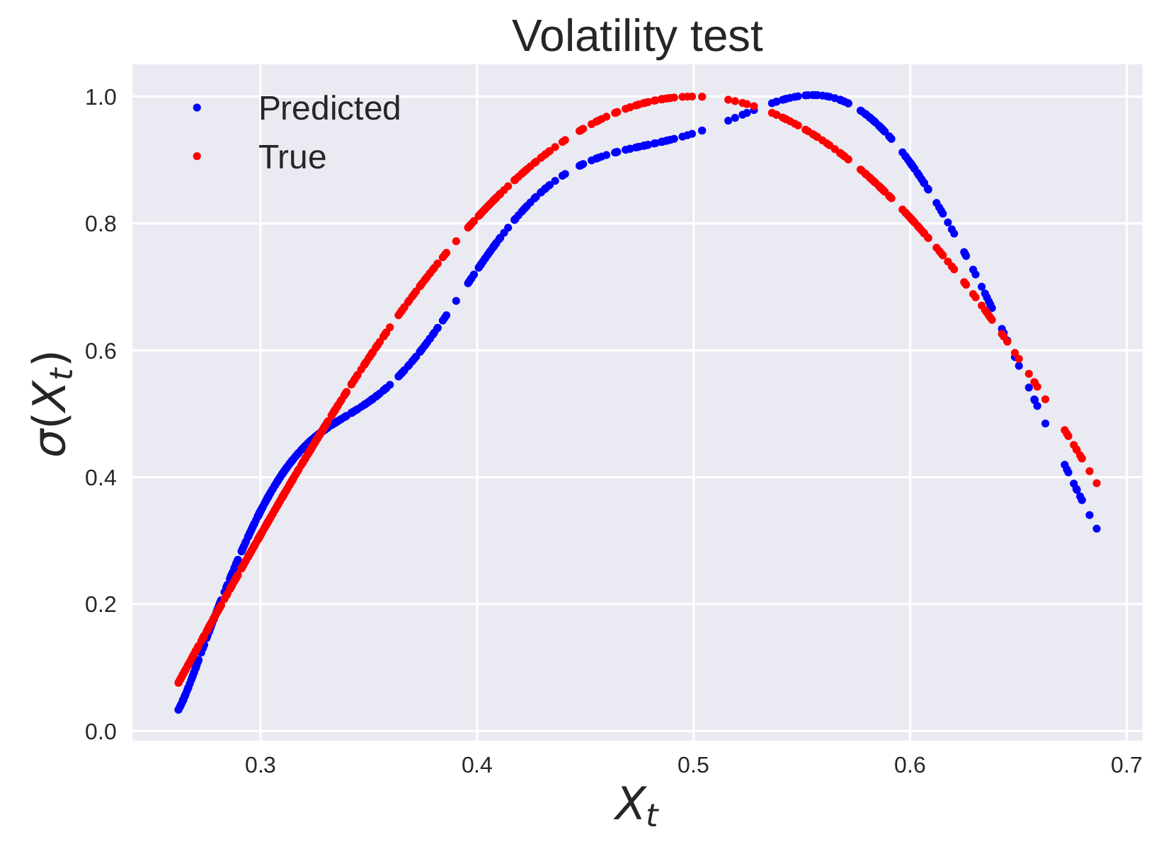
In this case, both the drift and volatility functions are non-linear functions of $X_{t}$. We generate two trajectories with volatility parameter $b=1.0,0.5$. For $b=0.5$, we set $\Delta t=0.01$. For the second trajectory, $b=0.5$ and the timestep is set $\Delta t=0.001$. In this case, the testing data contains points outside the training distribution. Hence the problem of prediction is more challenging than the problem of recovery at the training points. The results for the learned and unlearned kernel are reported in table 2. The training and testing data are illustrated in figure 20. For trajectory 2, the optimization of the hyper-parameters of the kernel yield a better recovery and a better prediction of the volatility outside the training distribution 4, 5 (also see figures 5 in the appendix).

	Trajectory 1			Trajectory 2
	$\mathcal{L}(\bar{f}^{*},\bar{\sigma}^{*}|X,Y)$	$\delta_{f}$	$\delta_{\sigma}$	$\mathcal{L}(\bar{f}^{*},\bar{\sigma}^{*}|X,Y)$	$\delta_{f}$	$\delta_{\sigma}$
Benchmark	-3.411	0.327	0.442	-3.808	3.454	0.198
Non-learned kernel	-3.675	0.157	0.093	-2.405	0.832	0.665
Learned kernel	-3.678	0.269	0.088	-3.642	1.481	0.242

Table 2. Results for the trigonometric process.

Figure 4. From left to right: drift function, volatility function, sample trajectory and sample increments of the trigonometric process (trajectory 2).

Figure 5. Predicted drift and volatility on the testing set for trajectory 2 of the trigonometric process. From left to right: drift (non-learned kernel), volatility (non-learned kernel), drift (learned kernel), volatility (learned kernel) .

5.5.1. Benchmark comparison

Generally our method with optimized parameters outperforms our selected benchmark both in recovery of the drift and the volatility as measured by our metric. Because the standard Gaussian process regressor uses a white noise kernel, it generally does not capture well a non-constant volatility. Our method on the other hand is able to capture non-constant volatility models. Compare for example figures 5 and 7.

Figure 6. Exponential volatility process benchmark prediction. From left to right: drift (trajectory 1), volatility (trajectory 1), drift (trajectory 2), volatility (trajectory 2).

Figure 7. Trigonometric process benchmark prediction. From left to right: drift (trajectory 1), volatility (trajectory 1), drift (trajectory 2), volatility (trajectory 2).

6. Experimental results: a comparison between perfectly specified and non perfectly specified kernels.

We now illustrate how the choice of the kernel can have a significant impact on the recovery of the drift and volatility. The following examples illustrate how choosing from the correct parametric family of kernels can improve both the recovery and the prediction of the functions of interest.

6.0.1. Overcoming non perfectly specified kernels

We consider the Geometric Brownian Motion process defined as

$$dX_{t}=\mu X_{t}dt+\sigma X_{t}dW_{t}\quad\text{Geometric Brownian motion (GBM).}$$ (26)

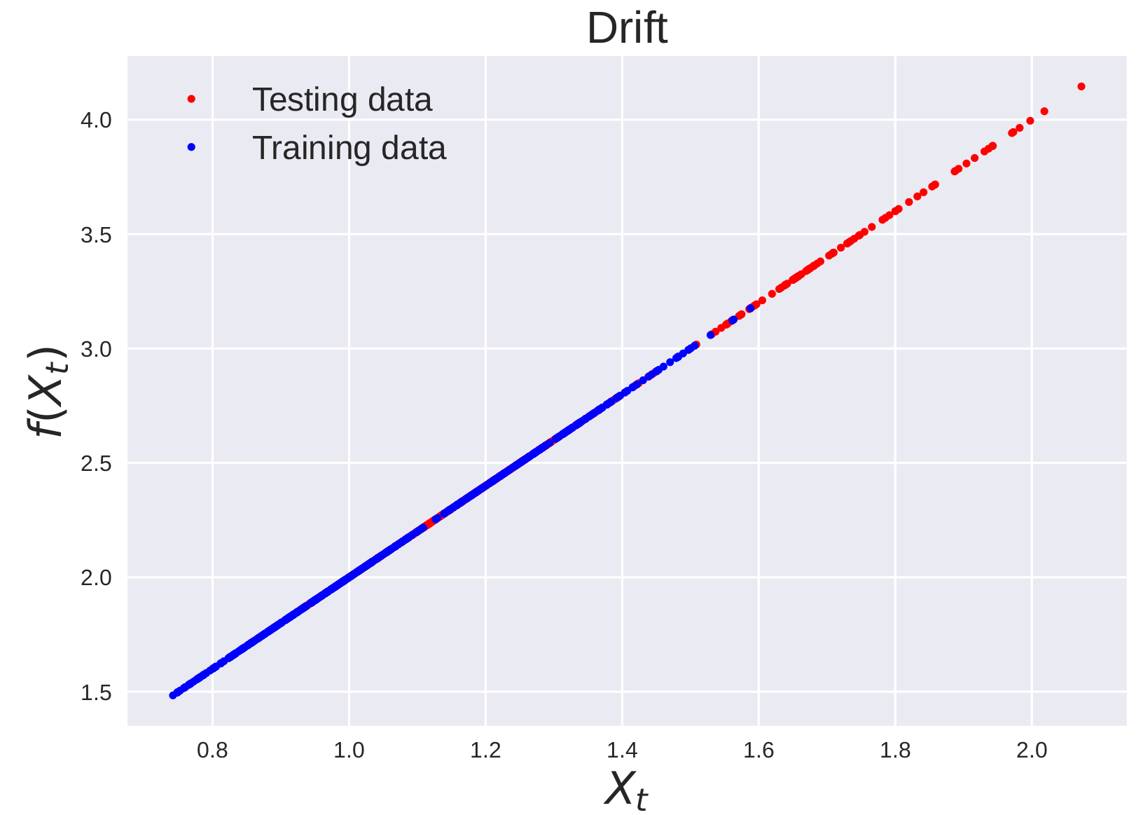
We generate one trajectory with parameters $\mu=2.0,\sigma=1.0$ and initial condition $X_{0}=1.0$, using the Euler-Maruyama discretization with timestep $\Delta t=0.001$. We focus primarily on the recovery of the volatility (the recovery of the drift is very difficult at a fine time-scale). The generated data is illustrated in figure 8.

Figure 8. From left to right: drift function, volatility function, sample trajectory, and sample increments of GBM.

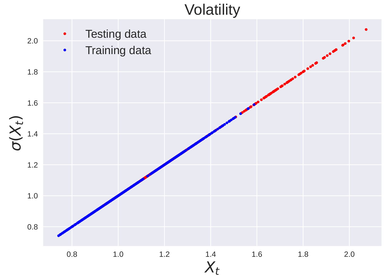
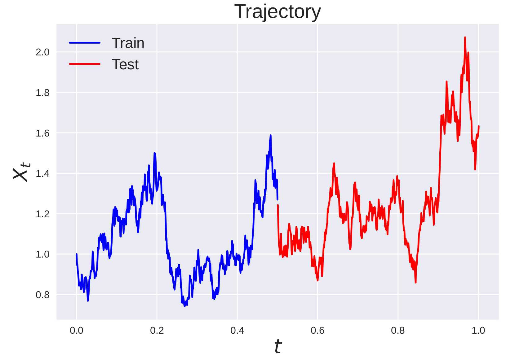
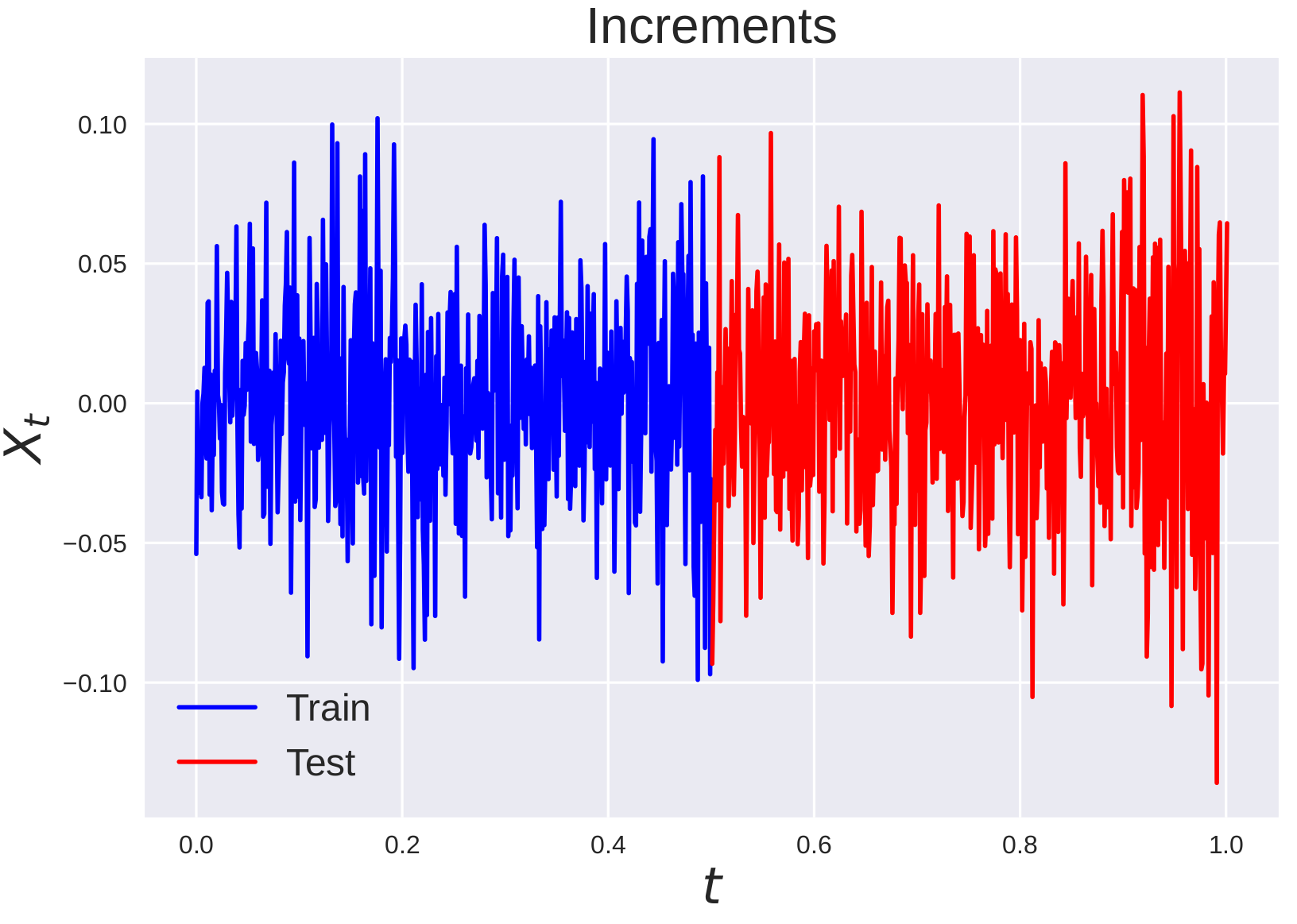
We compare the performance of the Matern kernel (21) family with the family of linear kernels [50] defined as

$$K_{\text{linear}}(x,y)=\sigma^{2}(x^{\intercal}y+c)$$ (27)

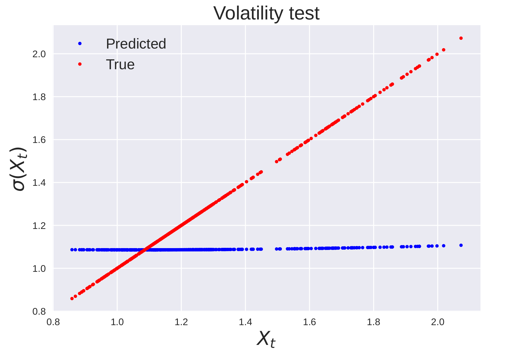
and parameterized by $(\sigma,c)$ which are learned. Note that this kernel induces the Reproducing Kernel Hilbert Space of linear functions and therefore is perfectly specified for GBM. The results are reported in table 3. The linear kernel is able to both recover and predict the volatility with or without learning the hyper-parameters, as it is perfectly specified for this problem. In contrast, without learning the hyper-parameters, the Matérn kernel is unable to accurately predict the future, reverting to the prior mean 0. Learning the hyper-parameters, however, enables the Matérn kernel to correctly predict future values. These results are illustrated in figure 9. We also observe that in all cases, our proposed approach outperforms the Gaussian Process Regressor benchmark (see figure 10).

	Linear kernel			Matern kernel
	$\mathcal{L}(\bar{f}^{*},\bar{\sigma}^{*}|X,Y)$	$\delta_{f}$	$\delta_{\sigma}$	$\mathcal{L}(\bar{f}^{*},\bar{\sigma}^{*}|X,Y)$	$\delta_{f}$	$\delta_{\sigma}$
Benchmark	-2.755	2.077	0.236	-2.755	2.018	0.237
Non-learned kernel	-2.800	0.763	0.015	-1.420	0.962	0.355
Learned kernel	-2.800	0.672	0.008	-2.800	0.500	0.010

Table 3. Comparison between the linear kernel and the Matern kernel on GBM.

Figure 9. Predicted volatility on the testing set for GBM. From left to right: linear kernel, Matern kernel (non-learned parameters) and Matern Kernel (learned parameters).

Figure 10. GBM benchmark prediction. From left to right: volatility (linear kernel) and volatility (Matern kernel).

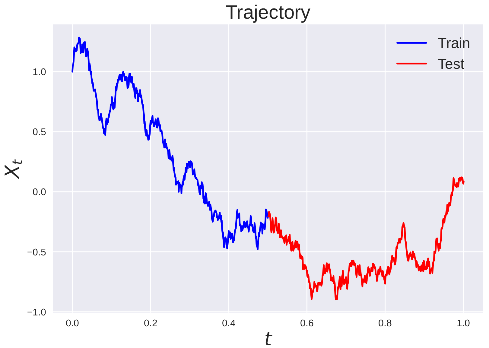
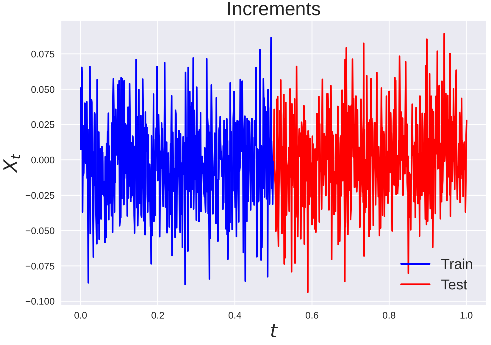
6.0.2. A failure case

We now present a case where our methodology fails because of a poor choice of prior. We consider the Ornstein–Uhlenbeck process defined as

$$dX_{t}=-\mu X_{t}dt+\sigma dWt,\quad\text{Ornstein–Uhlenbeck (OU).}$$

We discretize the process with parameters $\mu=-5$ and $\sigma=1.0$ and initial condition $X_{0}=1.0$ using the Euler-Maruyama method with a time discretization of $\Delta t=0.001$. One of the trajectories is illustrated in figure 11.

Figure 11. From left to right: drift function, volatility function, sample trajectory, and sample increments of the OU process.

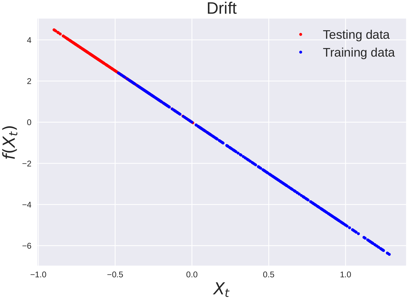
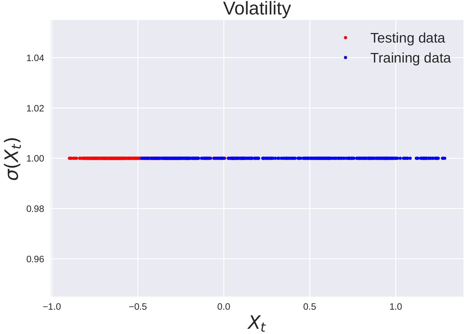
In this case, the drift is a linear function, and the volatility is a constant function. Hence a Matérn kernel prior is not perfectly specified. More precisely, the best prior for the volatility is a white noise kernel

$$K_{\text{wn}}(x,y)=\sigma^{2}\delta(x-y).$$ (28)

Therefore, in this case, the benchmark method (Gaussian process regression) is not only better specified than our method, but it is also optimal. We again use both the Matérn 21 and linear kernels (27). The results are presented in table 4. In this case, the benchmark always outperforms our computational graph completion approach in the recovery of the volatility. With a Matérn kernel our method outperforms the benchmark, but with a perfectly specified linear kernel, the benchmark outperforms our method. Moreover, figure 12 shows that the Matérn kernel does not capture the overall shape of the drift and volatility even if the relative error is low. We do note, however our cross-validation method improves the performance.

	Matérn kernel			Linear kernel
	$\mathcal{L}(\bar{f}^{*},\bar{\sigma}^{*}|X,Y)$	$\delta_{f}$	$\delta_{\sigma}$	$\mathcal{L}(\bar{f}^{*},\bar{\sigma}^{*}|X,Y)$	$\delta_{f}$	$\delta_{\sigma}$
Benchmark	-2.973	1.799	0.006	-2.977	0.212	0.006
Non-learned kernel	-2.971	1.038	0.065	-2.957	0.510	0.011
Learned kernel	-2.973	0.459	0.012	-2.978	1.066	0.013

Table 4. Results for the OU process.

Figure 12. Prediction on the OU process with the Matern kernel. From left to right: benchmark prediction (drift), benchmark prediction (volatility), CGC prediction (drift), CGC prediction (volatility).

Figure 13. Prediction on the OU process with the linear kernel. From left to right: benchmark prediction (drift), benchmark prediction (volatility), CGC prediction (drift), CGC prediction (volatility).

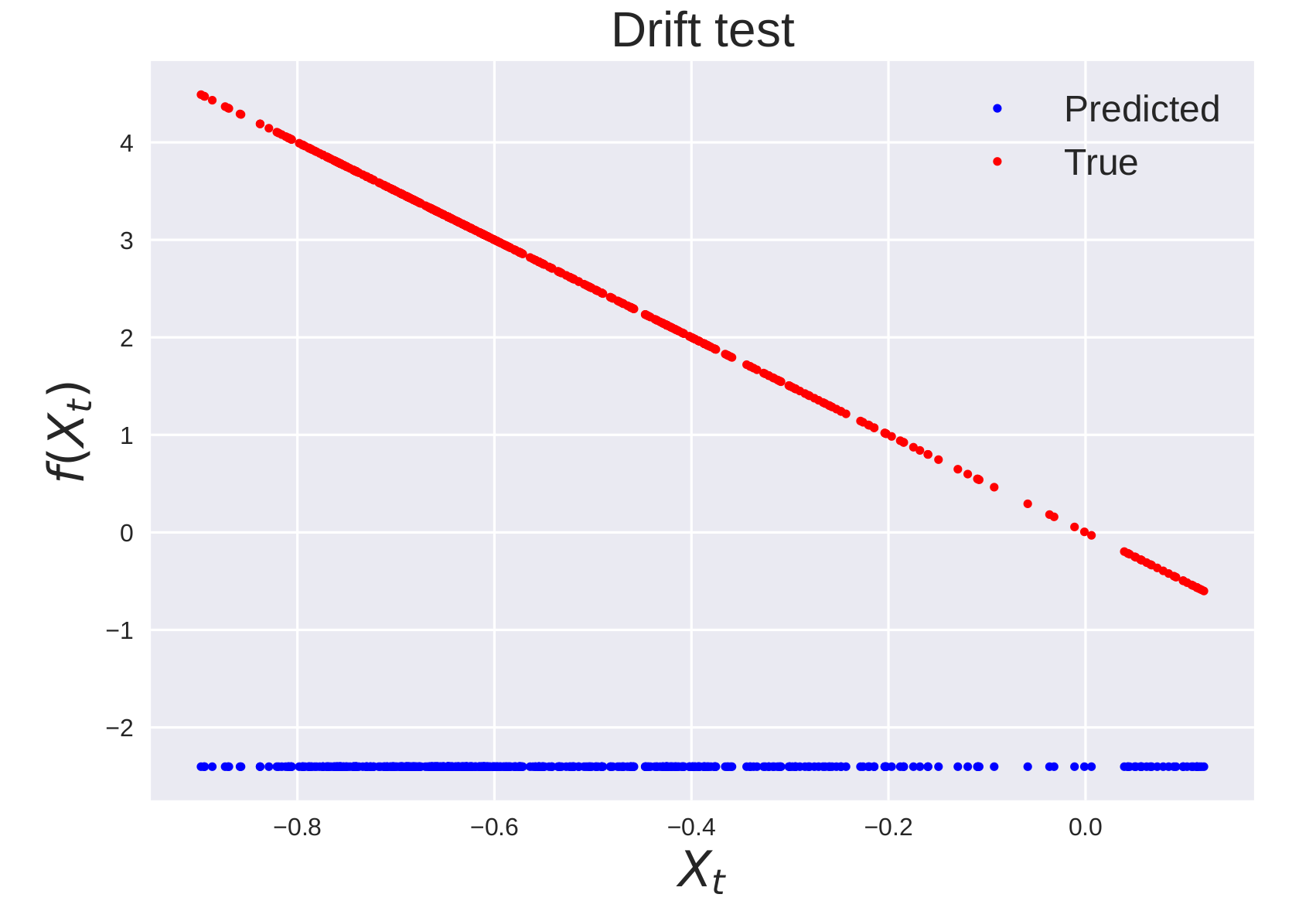
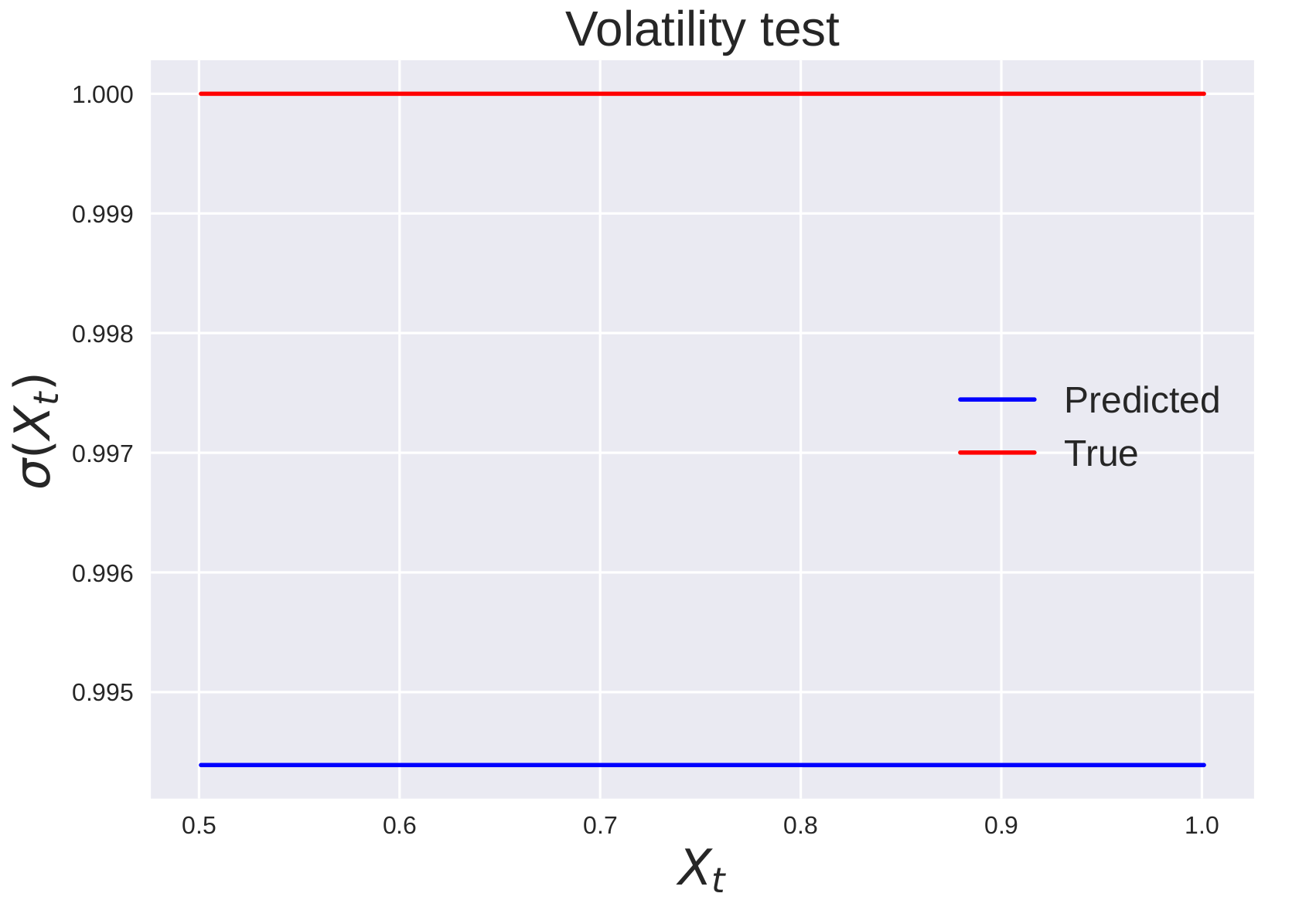
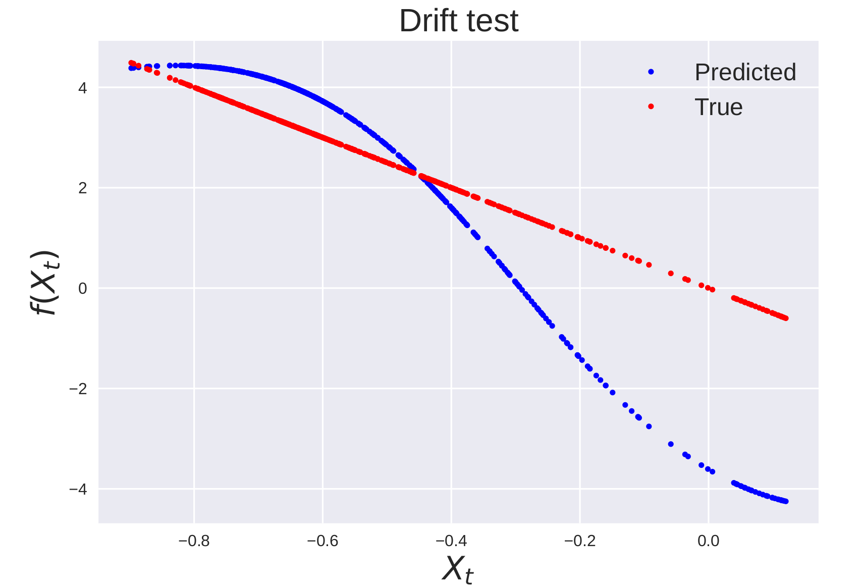
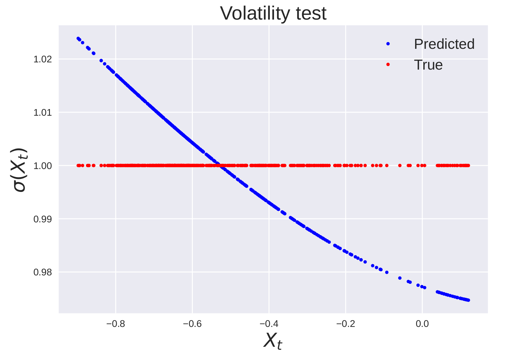
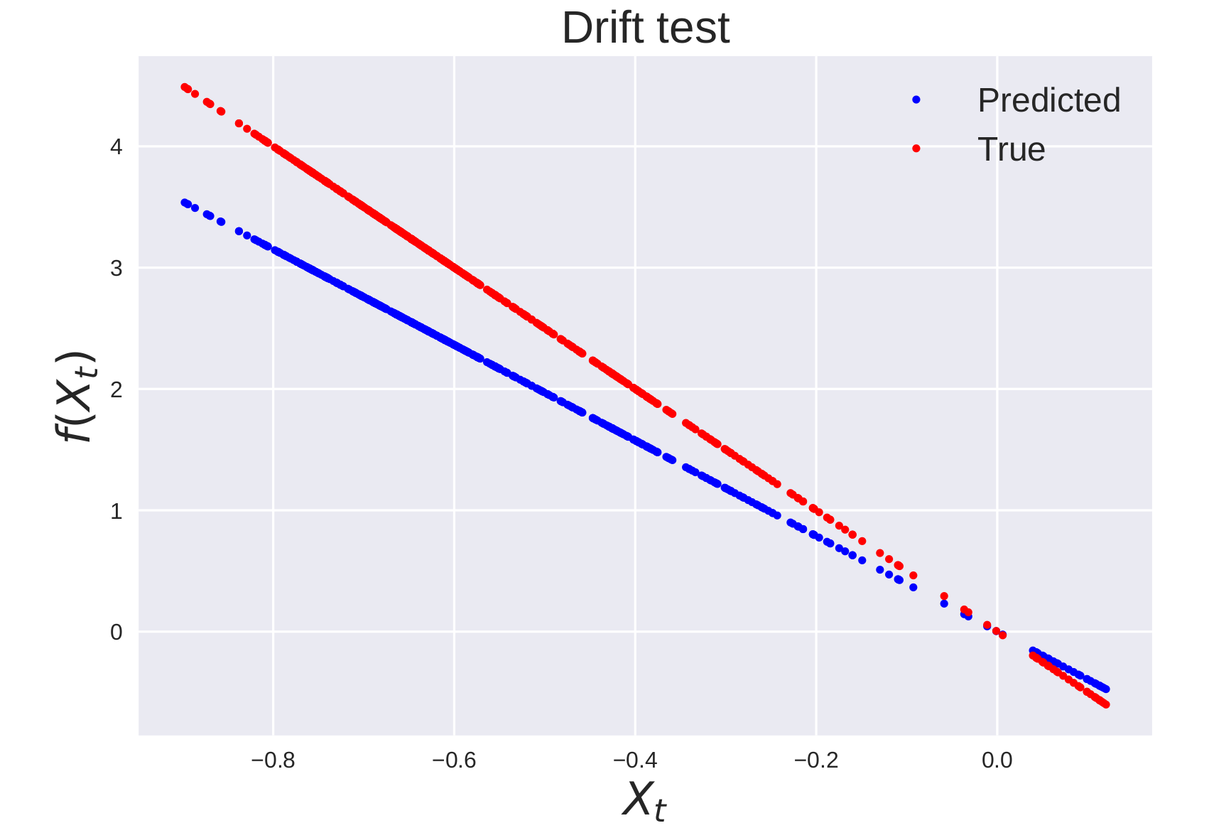
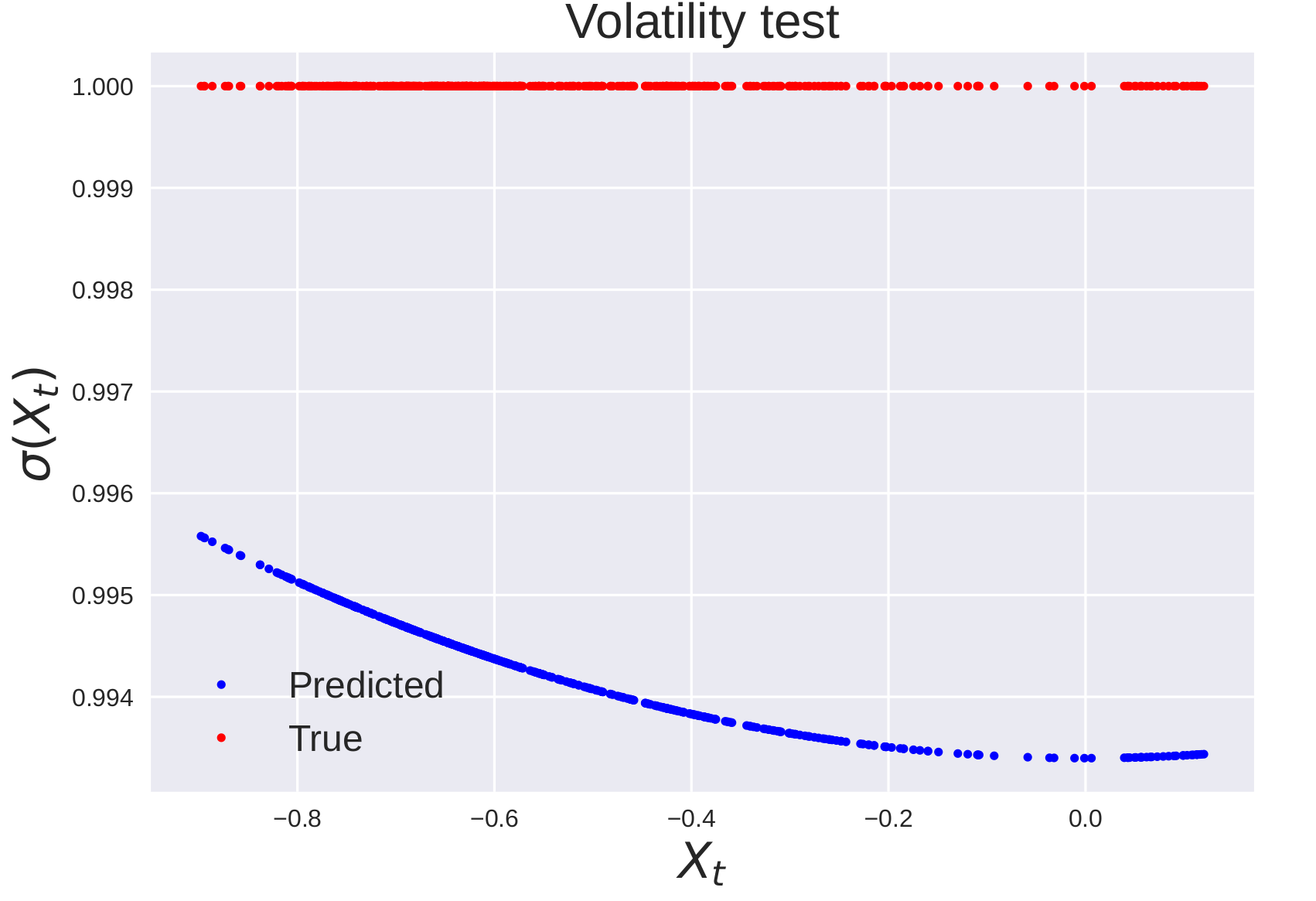
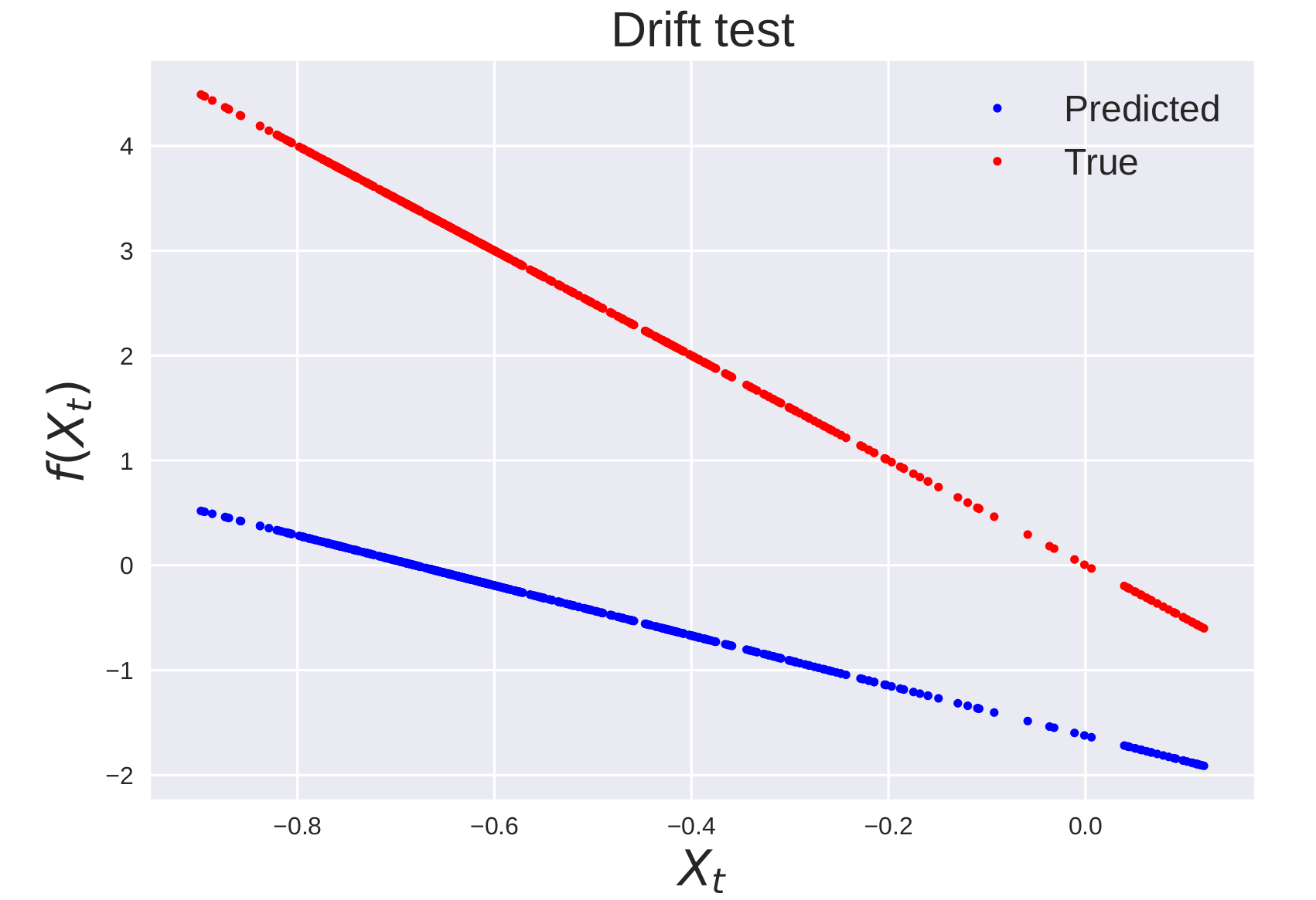
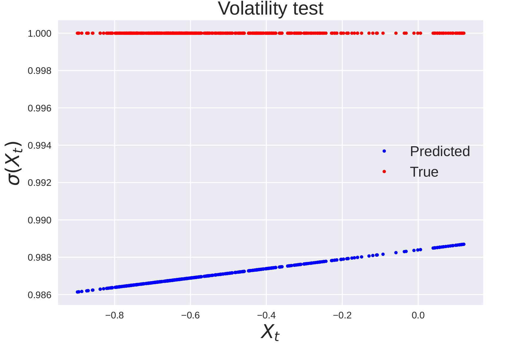
These results illustrate that choosing a perfectly specified kernel can improve the performance of the proposed method. Therefore, integrating prior knowledge such as the non-stationarity of the process into the choice of the prior can significantly improve performance. However, these results also illustrate how learning the parameters of a general kernel (such as the Matérn kernel) can yield similar performance to a well-specified kernel. A potential solution to this problem could be to learn a kernel which is the sum of a mix of stationary and non-stationary kernels such as

$$K_{\text{sum}}(x,y)=\sum_{i=1}^{N}\alpha_{i}K_{i}(x,y)$$ (29)

where the weights $\alpha_{i}$ are learned. Learning the weights of a sum of kernels is a well-established problem in the area of Support Vector Machines (see, for example [38]). Future avenues of research could therefore focus on efficient learning of hyper-parameters for this problem.

7. Experimental results: the effect of time discretization

We now examine the effect of time discretization. In all previous experiments, we observed the exact simulation of the trajectory. We now consider the cases where the observations do not exactly match the dynamics. More precisely, we generate a trajectory $(X_{i})_{i=1}^{M}$ separated by regular time steps $\Delta t$. We then consider the subs-trajectories $(X_{ik})_{ik=1}^{N}$ for $k=1,2,\dots,10$ where the indexes $ik$ are chosen such that $(X_{ik})_{ik=1}^{N}$ are separated by timesteps $k\times\Delta t$. This allows us to measure the impact of the discretization error on the effectiveness of our method. A priori, we would expect that our method would perform more poorly as $k$ grows larger, given that our modeling assumption is no longer fulfilled exactly.

We consider both our method with the initial guess of parameters (as detailed in the benchmark section 5.3) and with the optimized version of parameters. We also choose a base $\lambda$ which performs well for $k=1$ and set $\lambda_{k}=k\lambda$ for other values of $k$.

7.1. Exponential decay volatility.

We first consider the exponential decay volatility process described by (24) with time discretization $\Delta t=0.01$. For each $k$, we set $N=500$ for both the training and test sets. The results for $k$ are presented in table 5 and illustrative examples are presented in figures 14 and 15. We note that the choice of the Matérn kernel for the drift function induces a large error. A better choice of the kernel (such as the linear kernel discussed in section 6) would yield a better performance.

	Non optimized parameters			Optimized parameters
	$\mathcal{L}(\bar{f}^{*},\bar{\sigma}^{*}|X,Y)$	$\delta_{f}$	$\delta_{\sigma}$	$\mathcal{L}(\bar{f}^{*},\bar{\sigma}^{*}|X,Y)$	$\delta_{f}$	$\delta_{\sigma}$
k = 1	-1.887	0.472	0.062	-1.887	0.889	0.033
k = 2	-1.872	0.669	0.299	-1.843	0.897	0.181
k = 3	-1.896	0.702	0.419	-1.888	0.881	0.415
k = 4	-1.871	0.886	0.505	-1.922	0.902	0.502
k = 5	37.778	0.805	0.370	-1.928	0.855	0.574
k = 6	-1.802	0.901	0.605	-1.928	0.982	0.590
k = 7	-0.356	0.880	0.641	-1.818	0.865	0.638
k = 8	-1.774	0.913	0.505	-1.496	0.913	0.228
k = 9	-1.044	0.878	0.249	-1.881	0.919	0.659
k = 10	-1.648	0.940	0.439	-1.883	0.952	0.695

Table 5. Results for the exponential decay process for different time step $\Delta t$ observations.

Figure 14. Exponential decay volatility process: prediction of the volatility for different values of $k$. From left to right: $k=1,2,5$.

Figure 15. Exponential decay volatility process: prediction of the drift for different values of $k$. From left to right: $k=1,2,5$.

7.2. Trigonometric process

We now consider the trigonometric process described by (25) with time discretization $\Delta t=0.001$. For each $k$, we set $N=500$ for both the training and test sets. The results for $k$ are presented in table 6 and illustrative examples are presented in figures 16 and 17.

	Non optimized parameters			Optimized parameters
	$\mathcal{L}(\bar{f}^{*},\bar{\sigma}^{*}|X,Y)$	$\delta_{f}$	$\delta_{\sigma}$	$\mathcal{L}(\bar{f}^{*},\bar{\sigma}^{*}|X,Y)$	$\delta_{f}$	$\delta_{\sigma}$
k = 1	-3.675	0.259	0.093	-3.674	0.163	0.092
k = 2	-3.883	0.717	0.300	-3.807	0.792	0.299
k = 3	-3.729	0.702	0.419	-3.725	0.654	0.434
k = 4	-3.784	0.836	0.499	-3.798	0.848	0.495
k = 5	-4.027	0.904	0.587	-4.019	0.852	0.593
k = 6	-3.910	0.911	0.594	-3.942	0.952	0.597
k = 7	-3.909	0.954	0.636	-3.562	0.925	0.211
k = 8	-3.652	0.772	0.668	-3.930	0.767	0.669
k = 9	-3.939	0.880	0.657	-3.424	0.935	0.145
k = 10	-3.505	0.888	0.254	-3.926	0.880	0.705

Table 6. Results for the trigonometric process for different time step $\Delta t$ observations.

Figure 16. Trigonometric process: prediction of the volatility for different values of $k$. From left to right: $k=1,2,3$.

Figure 17. Trigonometric process: prediction of the drift for different values of $k$. From left to right: $k=1,2,5$.

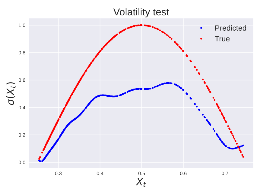
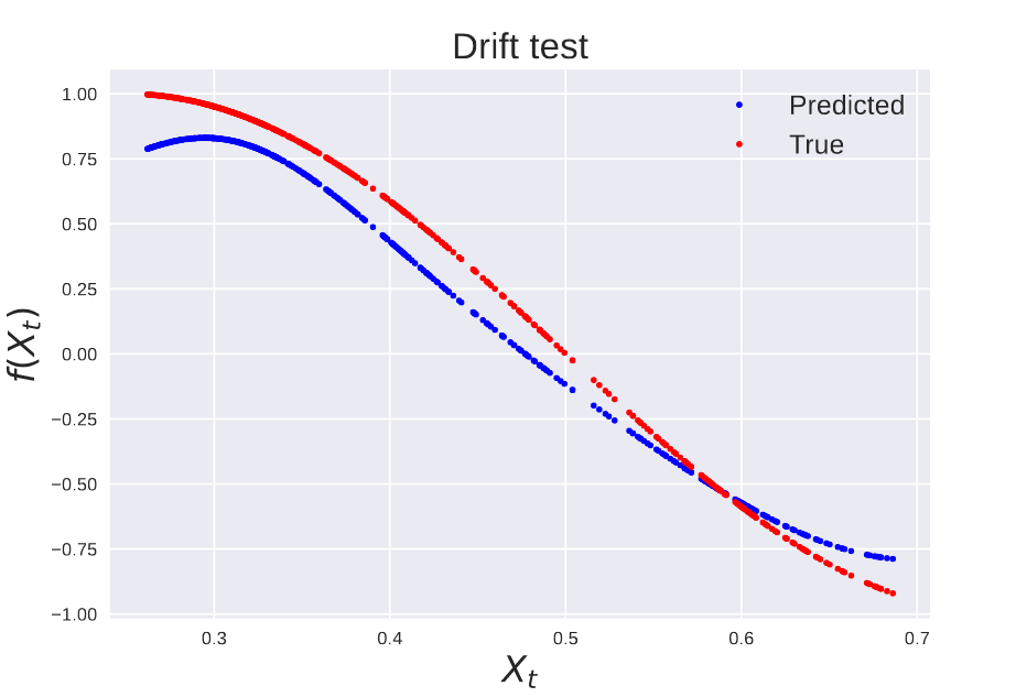
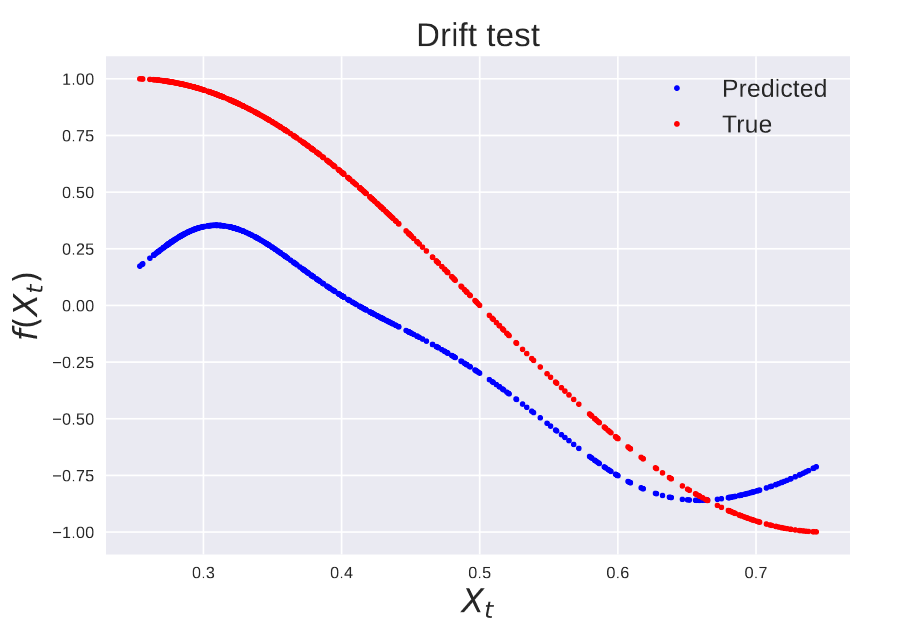
In general, we note that, as expected, as $k$ gets larger, our method has worse performance. Moreover, for values of $k\neq 1$, our cross-validation method does not perform as well, suggesting the need to adapt the cross-validation procedure to learning the parameter $\lambda$. There are, however some exceptions, such $k=8,9$ for the exponential volatility process and $k=7,9$ for the trigonometric process where one of the functions is better recovered. This suggests that a good choice of parameters via cross -validation leads to a good recovery even if the modeling assumption is incorrect, consistent with observations that cross-validation methods are somewhat robust to model misspecification [17].

8. Experimental results: discussion

We make the following observations regarding our results.

First, we observe that our method provides comparable or greater performance compared to simple kernel regression with hyper-parameters optimized through the minimization of the log marginal likelihood. Which method is preferable depends on the underlying SDE. We observe that for SDEs with constant volatility functions, such as the Ornstein–Uhlenbeck process, the simple kernel regression generally outperforms our method as measured by the likelihood. This is likely due to the better recovery of the volatility as the modeling assumption of the kernel regression (i.i.d. noise) better captures the true model (constant volatility). Nonetheless, our method does occasionally outperform kernel regression in predicting the drift of the SDE. Our method, however, notably outperforms kernel regression for SDEs with non-constant volatility, such as the trigonometric process and the exponential volatility process.

Second, we observe that the randomized cross-validation algorithm for hyper-parameter optimization reliably improves the performance of our method. In all cases, the selected parameters have better performance compared to the initial guess, as measured by the likelihood of the model. Moreover, as the Geometric Brownian Motion example illustrates, learning the parameters of the kernels can enable ill-specified kernels to perform comparably to well-specified kernels.

We also observe that a better likelihood generally implies a better capture of the drift and volatility. Hence, while these quantities are unobserved, better performance as measured by the likelihood generally implies that the model captures well both the drift and volatility.

Finally, we note that as the observations increasingly depart from the true dynamics, our method performs more poorly. This suggests the need for a better model for the discretization error term, either through learning the parameter $\lambda$ or a better modeling assumption than the i.i.d Gaussian noise presented in section 2.

Appendix A Additional Plots.

In this section, we provide additional plots of the results of the numerical experiments.

A.1. Exponential volatility process

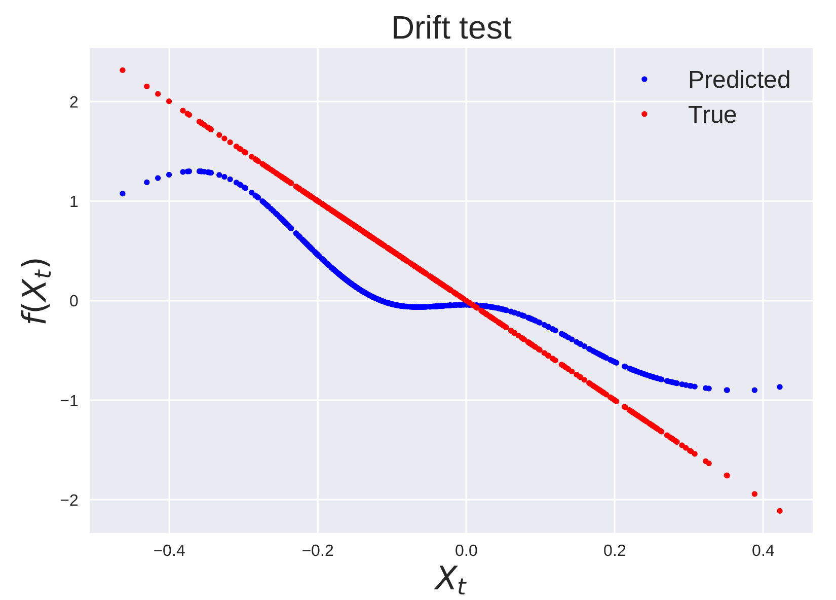
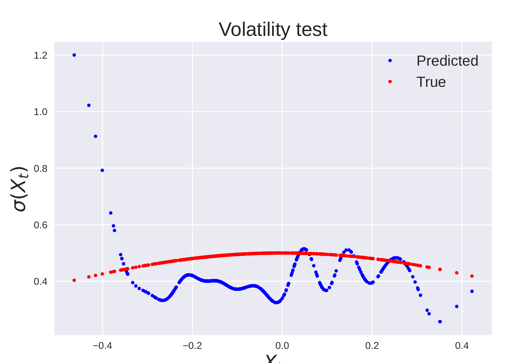
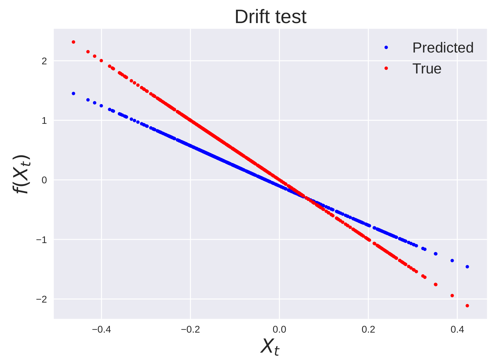
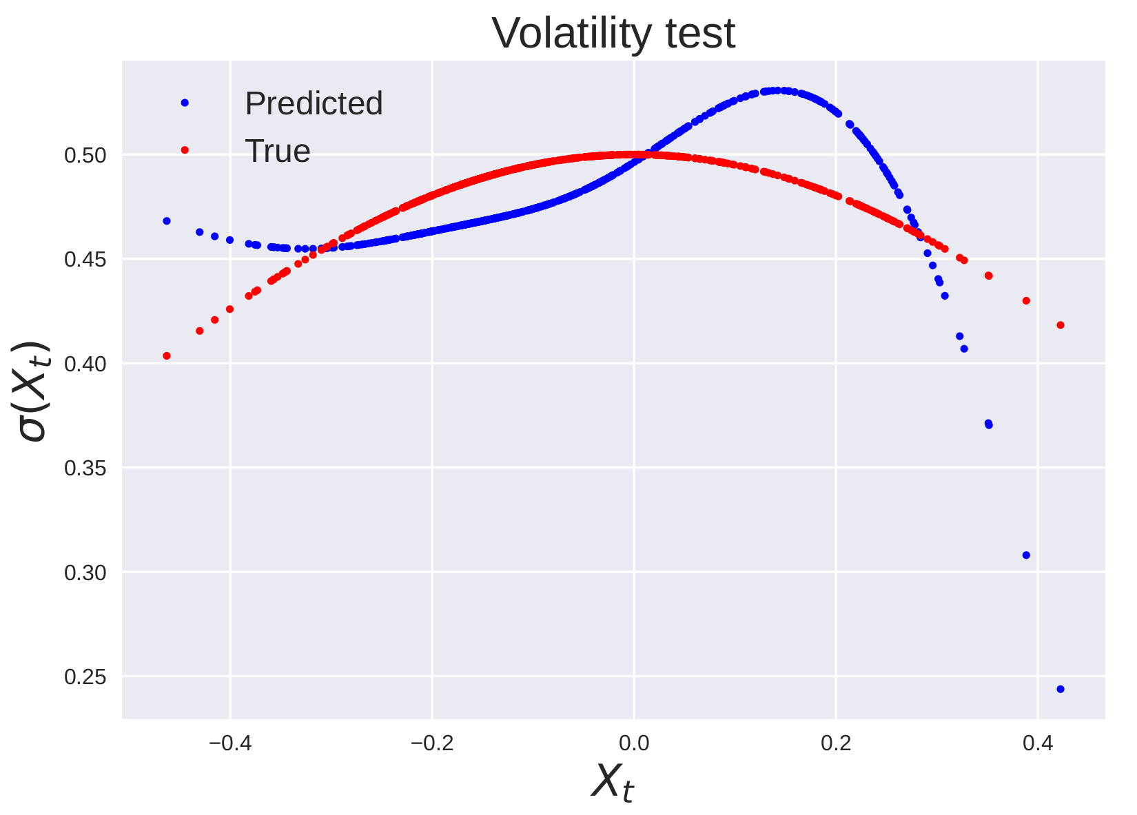
The following figures illustrate the results on the second trajectory of the exponential volatility process.

Figure 18. From left to right: drift function, volatility function, sample trajectory, and sample increments of the exponential volatility process.

Figure 19. Predicted drift and volatility on the testing set for trajectory 1 of the exponential volatility process. From left to right: drift (non-learned kernel), volatility (non-learned kernel), drift (learned kernel), volatility (learned kernel) .

A.2. Trigonometric process

The following figures illustrate the results of the first trajectory of the trigonometric process.

Figure 20. From left to right: drift function, volatility function, sample trajectory, and sample increments of the trigonometric process.

Figure 21. Predicted drift and volatility on the testing set for trajectory 1 of the trigonometric process. From left to right: drift (non-learned kernel), volatility (non-learned kernel), drift (learned kernel), volatility (learned kernel) .

Appendix B Gaussian Process Regression and Extension of [7, Page 306]

In this section, we give a very brief overview of Gaussian processes for regression. We suppose that the values of $Y(X)$ are distributed according to a Gaussian process, namely $Y(X)\overset{d}{\sim}\mathcal{GP}(\boldsymbol{O},\boldsymbol{K})$. In particular, in the case of SDEs, given the data $(X,Y)$, the predicted drift and diffusion for a new point $x_{*}$ are given by

$$\bar{f}(x_{*})=K(x_{*},X)K(X,X)^{-1}Y$$

$$\bar{\sigma}(x_{*})=K(x_{*},x_{*})-K(x_{*},X)K(X,X)^{-1}K(X,x_{*})$$

The above expressions are valid in noisy observation with independent and identical Gaussian noise. We derive this distribution in the case where the observations are noisy with independent, but not necessarily identical, Gaussian noise; the proof is generalized from the one presented in [7, 306].
Formally, suppose that we have at our disposal the noisy observations $(X_{n},Y_{n})_{1\leq n\leq N}$, where $Y_{i}=f(X_{i})+W_{i}$ and the $W_{i}$ are independent but not necessarily identically distributed $\mathcal{N}(0,\sigma^{2}(X_{i}))$ random variables. The problem is the identification of the unknown function $f$ given these noisy observations. Set $f_{i}=f(X_{i})$, so that $\boldsymbol{f}:=(f_{i})_{1\leq i\leq N}$. In addition, set $\boldsymbol{Y}:=(Y_{i})_{1\leq i\leq N}$. Observe that $\boldsymbol{Y}|\boldsymbol{f}\overset{d}{\sim}\mathcal{N}(\boldsymbol{f},\boldsymbol{\Sigma})$ where $(\,\Sigma\,)_{ij}=\delta_{ij}\sigma^{2}(X_{i})$, and assume that $\boldsymbol{f}\overset{d}{\sim}\mathcal{N}(\boldsymbol{0},\boldsymbol{K})$. Then, [7, Page 93],

$$p(\boldsymbol{Y})=\int p(\boldsymbol{Y}|\boldsymbol{f})p(\boldsymbol{f})d\boldsymbol{f}=\mathcal{N}(\boldsymbol{0},\boldsymbol{K+\Sigma}).$$

Now, let $\boldsymbol{C}=\boldsymbol{K+\Sigma}$ so that $\boldsymbol{C}_{ij}=k(X_{i},X_{j})+\sigma_{i}^{2}\delta_{ij}$. Denote $\boldsymbol{Y}_{N+1}=(Y_{1},...,Y_{N+1})$, $\boldsymbol{Y}_{N}=(Y_{1},...,Y_{N})$. We wish to derive the conditional distribution $p(Y_{N+1}|\boldsymbol{Y}_{N})$. First, observe that

$$p(\boldsymbol{Y}_{N+1})=\mathcal{N}(\boldsymbol{0},\boldsymbol{C}_{N+1}).$$

where $\boldsymbol{C}_{N+1}$ is the $(N+1)\times(N+1)$ with entries defined as previously for the vector $\boldsymbol{Y}_{N+1}$. We may partition the covariance matrix as

$$\boldsymbol{C}_{N+1}=\begin{pmatrix}\boldsymbol{C}_{N}&\boldsymbol{K}\\ \boldsymbol{K}^{T}&c\end{pmatrix}$$

where $c=K(X_{N+1},X_{N+1})+\sigma_{N+1}^{2}$ and $\overline{\boldsymbol{K}}$ is the vector with entries $\overline{\boldsymbol{K}}_{i}=K(X_{N+1},X_{i})$. Then $p(Y_{N+1}|\boldsymbol{Y}_{N})=\mathcal{N}(m(X_{N}),\sigma^{2}(X_{N}))$ and the conditional mean and covariance are given by

$$m(X_{N+1})=\overline{\boldsymbol{K}}^{T}\boldsymbol{C}^{-1}\boldsymbol{y}_{N}=\overline{\boldsymbol{K}}^{T}(\boldsymbol{K+\Sigma})^{-1}\boldsymbol{y}_{N}$$

$$\sigma^{2}(X_{N})=c-\overline{\boldsymbol{K}}^{T}\boldsymbol{C}^{-1}\overline{\boldsymbol{K}}=c-\overline{\boldsymbol{K}}^{T}(\boldsymbol{K+\Sigma})^{-1}\overline{\boldsymbol{K}}.$$

Note that in our case, the observations actually of the form $Y_{i}=\Delta t_{i}f(X_{i})+W_{i}$. The same proof holds with the slight modification that the entries of the covariance matrix now become

$$\boldsymbol{C}_{ij}=\Delta t_{i}\Delta t_{j}k(X_{i},X_{j})+\sigma_{i}^{2}\delta_{ij}$$

$$\overline{\boldsymbol{K}}_{i}=\Delta t_{i}K(X_{N+1},X_{i})$$

which yields equations (7) and (8).

Appendix C Log-marginal likelihood for hyper-parameter optimization

In this section, we briefly present the log-marginal likelihood method for hyper-parameter optimization. The marginal log-likelihood over the kernel parameters can be expressed as:

$$-\log(p(Y|\boldsymbol{\theta},X))\propto\frac{1}{2}Y^{T}K(X,X)^{-1}Y+\log(|K(X,X)|).$$

Therefore, the optimal parameters $\boldsymbol{\theta}$ are obtained via the minimization of the function in the previous equation (with respect to $\boldsymbol{\theta}$). In the case of noisy observations, the kernel $K$ can be defined as

$$K(X_{1},X_{2})=K^{{}^{\prime}}(X_{1},X_{2})+\delta(X_{1},X_{2})$$

where $K^{\prime}$ is a standard kernel and $\delta$ is the white noise kernel defined as

$$\delta(X_{1},X_{2}):=\begin{cases}c&\text{if}\;X_{1}=X_{2},\\ 0&\text{otherwise},\end{cases}$$

where $c$ is the noise level, a kernel parameter that must be optimized. It is important to note that this kernel can only account for a constant level of noise, which is not the case for many SDEs.

Appendix D Randomized cross-validation for hyper-parameter learning

In this section, we describe the general framework of Randomized cross-validation we use in our optimization.
The general problem is the following: we have a set of training data $(\boldsymbol{X},Y):=\{(X_{i},Y_{i})\}_{1\leq i\leq N}$ and we are trying to recover a function $f:\boldsymbol{X}\rightarrow Y$. In particular, we assume that we have a class of functions $\mathcal{S}$ indexed by a set of parameters $\boldsymbol{w}_{p}\in\mathcal{W}$, i.e. $\mathcal{S}:=\{f(\,\cdot\,,\boldsymbol{w}_{p})\,:\,\boldsymbol{w}_{p}\in\mathcal{W}\,\,\text{and}\,\,f(\,\cdot\,,\boldsymbol{w}_{p}):\boldsymbol{X}\rightarrow Y\}$. Notice that in practice, this could be approximated via reproducing kernels as in this paper or via neural networks. We assume that we have a method to find the optimal parameter $\boldsymbol{w}^{*}_{p}\in\mathcal{W}$ for a given training set of data $(\boldsymbol{X},Y)$. In our case, we assume that such a method involves the minimization of some loss function $\mathcal{L}(f(\boldsymbol{X},\boldsymbol{w_{p}}),Y)$ with respect to $\boldsymbol{w}_{p}$, where $\mathcal{L}\,:\,Y\times Y\rightarrow\mathbb{R}$. Moreover, like in many Machine Learning (ML) algorithms, we assume that we have a set of hyper-parameters $\boldsymbol{\theta}\in\boldsymbol{\Theta}$ that affect the recovery of the optimal $\hat{f}\in\mathcal{S}$. Such hyper-parameters $\boldsymbol{\theta}$ can parametrize the function $\hat{f}:=\hat{f}_{\boldsymbol{\theta}}:=f(\,\cdot\,;\boldsymbol{w}_{p},\boldsymbol{\theta})$, regularize the loss function $\mathcal{L}$ (often through some prior distribution on the parameters $\boldsymbol{w}_{p}$) or affect the minimization of the loss $\mathcal{L}$ (such as the learning rate of a gradient descent). We summarize this point by saying that $\hat{f}$ is recovered by minimizing $\mathcal{L}_{\boldsymbol{\theta}}$.
In the present work, in order to recover the function $f:\boldsymbol{X}\rightarrow Y$, we apply the Robust Learning Algorithm, whose rationale is explained in the following paragraph.

Robust Learning Algorithm via Randomized cross-validation.

Many ML algorithms are built upon minimizing a loss function $\mathcal{L}:Y\times Y\rightarrow\mathbb{R}$ over the set of parameters $(\boldsymbol{w}_{p},\boldsymbol{\theta})$ of a class of models $\hat{f}\left(\,\cdot\,,\boldsymbol{w}_{p};\boldsymbol{\theta}\right)$. In other words, ideally, we can define the risk function $R$ as the expected value of the loss function $\mathcal{L}$ with respect to the data probability density function $p\left(\boldsymbol{x},y\right)$:

$$R\left(\boldsymbol{w}_{p},\boldsymbol{\theta}\right):=\mathbb{E}_{(\boldsymbol{X},Y)\sim p\left(\boldsymbol{x},y\right)}\left\{\mathcal{L}\left(\hat{f}(\boldsymbol{X},\boldsymbol{w}_{p};\boldsymbol{\theta}),Y\right)\right\}$$ (30)

and then find the set of optimal parameters according to

$$\left(\boldsymbol{w}_{p}^{*},\boldsymbol{\theta}^{*}\right):=\underset{\boldsymbol{w}_{p},\boldsymbol{\theta}}{\arg\min}\,\,R\left(\boldsymbol{w}_{p},\boldsymbol{\theta}\right).$$ (31)

Notice that, in this setup, by the assumption that one has access to $p\left(\boldsymbol{x},y\right)$, there is no theoretical distinction between parameters and hyper-parameters.
However, in practice, one only sees a realization of $\left(\boldsymbol{X},Y\right)$, namely $\mathcal{D}=\left\{\left(\boldsymbol{X}_{i},Y_{i}\right)\right\}_{i\in\mathcal{I}}$. Therefore, it is impossible to use Equations (30) and (31). Moreover, in order to achieve generalization, in practice, $\boldsymbol{w}_{p}$ is optimized by minimizing a loss function dependent on $\boldsymbol{\theta}$:

$$\boldsymbol{w}_{p}^{*}=\underset{\boldsymbol{w}_{p}}{\arg\min}\,\mathcal{L}_{\boldsymbol{\theta}}\left(\hat{f}\left(\boldsymbol{X};\boldsymbol{w}_{p},\boldsymbol{\theta}\right),Y\right)$$ (32)

At this point, the best parameters $\boldsymbol{\theta}$ can be chosen via a cross-validation approach where the function $\hat{f}_{\boldsymbol{\theta}}$ is evaluated on an unseen test set $(\boldsymbol{X_{u}},Y_{u})$:

$$R(\boldsymbol{\theta})=\mathcal{L}\left(\hat{f}\left(\boldsymbol{X}_{u};\boldsymbol{w}^{*}_{p},\boldsymbol{\theta}\right),Y_{u}\right)$$ (33)

Generally, the optimization of hyper-parameters [5, 6, 29, 54, 40, 22] is usually done on a prefixed number of cross validation sets. In this work, we propose an approach that is not bound to a fixed number of cross-validation sets. Our algorithm can be summarized as follows:

1. Partition the available data $\mathcal{D}=\left\{\left(\boldsymbol{X}_{i},Y_{i}\right)\right\}_{i\in\mathcal{I}}$ into a training subset $\mathcal{D}_{\mathcal{T}}=\left\{\left(\boldsymbol{X}_{i},Y_{i}\right)\right\}_{i\in\mathcal{T}}$ and a test subsets $\mathcal{D}_{\mathcal{U}}=\left\{\left(\boldsymbol{X}_{i},Y_{i}\right)\right\}_{i\in\mathcal{U}}$; the two subsets are mutually exclusive.

2. Randomly partition the training set $\mathcal{D}_{\mathcal{T}}$ into two mutually exclusive subsets of almost equal size: $\mathcal{D}_{\prod}=\left\{\left(\boldsymbol{X}_{i},Y_{i}\right)\right\}_{i\in\prod\left(\mathcal{T}\right)}$ and $\mathcal{D}_{\prod^{c}}=\left\{\left(\boldsymbol{X}_{i},Y_{i}\right)\right\}_{i\in\prod^{c}\left(\mathcal{T}\right)}$. Here, $\prod\left(\mathcal{T}\right)$ returns the first half of the random permutation of indices in $\mathcal{T}$ and $\prod^{c}\left(\mathcal{T}\right)$ returns the second half of the same permutation.

3. Train a ML model on $\mathcal{D}_{\prod}$ and evaluate the random loss on $\mathcal{D}_{\prod^{c}}$ representing a realization of the generalization error.

4. Repeat steps (2) and (3) to optimize the expected loss over the random sets $\mathcal{D}_{\prod^{c}}$ with respect to $\boldsymbol{w}_{p}$.

5. Check the goodness of fit by evaluating the loss over $\mathcal{D}_{\mathcal{U}}$.

More precisely, the optimization problem is the following one:

$$\begin{array}[]{ll}&\boldsymbol{\theta}^{*}=\underset{\boldsymbol{\theta}}{\arg\min}\,\,\mathbb{E}_{\varPi}\left\{R_{\mathbb{I}-\prod}\left(\bar{\boldsymbol{w}}_{p},\boldsymbol{\theta}\right)\right\}\\ \text{\,\,\,\,\,\,\,\,\,\,\,\,\,\,\, s.t.}&\bar{\boldsymbol{w}}_{p}=\underset{\boldsymbol{w}_{p}}{\arg\min}\,\,R_{\prod}\left(\boldsymbol{w}_{p},\boldsymbol{\theta}\right).\end{array}$$ (34)

Where,

$$R_{\prod}\left(\boldsymbol{w}_{p},\boldsymbol{\theta}\right)=\mathbb{E}_{\boldsymbol{X},Y\sim\mathcal{D}_{\prod}}\left\{\mathcal{L}_{\boldsymbol{\theta}}\left(\hat{f}\left(\boldsymbol{X};\boldsymbol{w}_{p},\boldsymbol{\theta}\right),Y\right)\right\},$$ (35)

and

$$R_{\mathbb{I}-\prod}\left(\boldsymbol{w}_{p},\boldsymbol{\theta}\right)=\mathbb{E}_{\boldsymbol{X},Y\sim\mathcal{D}_{\prod^{c}}}\left\{\mathcal{L}\left(\hat{f}\left(\boldsymbol{X};\boldsymbol{w}_{p},\boldsymbol{\theta}\right),Y\right)\right\}.$$ (36)

In the previous Equations, $\mathbb{E}_{\boldsymbol{X},Y\sim\mathcal{D}_{\prod}}\left\{\,.\,\right\}$ means that the expected value is taken over the empirical distribution defined by $\mathcal{D}_{\prod}$. A similar notion applies to $\mathbb{E}_{\boldsymbol{X},Y\sim\mathcal{D}_{\prod^{c}}}\left\{\,.\,\right\}$. Furthermore, $\mathbb{E}_{\varPi}\left\{\,.\,\right\}$ means that this expected value is taken over all permutations of the train set. Note that the recovery of $\bar{\boldsymbol{w}}_{p}$ is done through the minimization of $\mathcal{L}_{\boldsymbol{\theta}}$ which we refer to as the train loss function, whereas the evaluation of $\hat{f}\left(\boldsymbol{X};\boldsymbol{w}_{p},\boldsymbol{\theta}\right)$ is done through $\mathcal{L}$ which we refer to as the test loss function. The Robust Learning Algorithm is presented here below in (1):

Algorithm 1 Robust Learning Algorithm

 

1. Pick a model class $\hat{f}_{\boldsymbol{\theta}}$

2. Pick an initial guess $\boldsymbol{\theta}^{\left(0\right)}$.

3. Pick an active learning algorithm Al.

4. Set $\mathcal{S}=\phi$, $n=0$ and $C=0$.

Partition the data $\mathcal{D}=\left\{\left(\boldsymbol{x}_{i},y_{i}\right)\right\}_{i\in\mathcal{I}}$ into two mutually exclusive training $\mathcal{D}_{\mathcal{T}}=\left\{\left(\boldsymbol{x}_{i},y_{i}\right)\right\}_{i\in\mathcal{T}}$ and test subsets $\mathcal{D}_{\mathcal{U}}=\left\{\left(\boldsymbol{x}_{i},y_{i}\right)\right\}_{i\in\mathcal{U}}$.

while $C=0$ do

     $n\leftarrow n+1$

     while $1\leq j\leq K$ do

         $j\leftarrow j+1$

         Pick a random index permutation $\prod_{n}\left(\mathcal{T}\right)$ of $\mathcal{T}$.

         Divide the train set $\mathcal{D}_{\mathcal{T}}$ into $\mathcal{D}_{\prod_{n}}$ and $\mathcal{D}_{\prod_{n}^{c}}$.

         Train $\hat{f}\left(\boldsymbol{X};\boldsymbol{w}_{p},\boldsymbol{\theta}^{\left(n-1\right)}\right)$ on $\mathcal{D}_{\prod_{n}}$ with respect to $R_{\prod_{n}}\left(\boldsymbol{w}_{p},\boldsymbol{\theta}^{\left(n-1\right)}\right)$ to obtain $\bar{\boldsymbol{w}}_{p}$.

         Evaluate $e_{j}=R_{\mathbb{I}-\prod_{n}}\left(\bar{\boldsymbol{w}}_{p},,\boldsymbol{\theta}^{\left(n-1\right)}\right)$ on $\mathcal{D}_{\prod_{n}^{c}}$.

     end while

     Set $R_{\mathbb{I}-\prod_{n}}=\frac{1}{K}\sum_{j=1}^{K}e_{j}$.

     Set $\mathcal{S}\leftarrow\mathcal{S}\cup\left\{\left(\boldsymbol{\theta}^{\left(n-1\right)},R_{\mathbb{I}-\prod_{n}}\left(\bar{\boldsymbol{w}}_{p},,\boldsymbol{\theta}^{\left(n-1\right)}\right)\right)\right\}$.

     

     if $Al\left(\mathcal{S}\right)$ has converged then

         $C=1$

         $\left(\boldsymbol{w}_{p}^{*},\boldsymbol{\theta}^{*}\right)=\left(\bar{\boldsymbol{w}}_{p},,\boldsymbol{\theta}^{\left(n-1\right)}\right)$.

     else if $Al\left(\mathcal{S}\right)$ has not converged then

         $\boldsymbol{\theta}^{\left(n\right)}=Al\left(\mathcal{S}\right)$

     end if

end while

Check the loss over $\mathcal{D}_{\mathcal{U}}$.

In particular, notice that $R_{\mathbb{I}-\prod_{n}}=\frac{1}{K}\sum_{j=1}^{K}e_{j}$ is a (noisy) approximation of

$$\mathbb{E}_{\boldsymbol{X},Y\sim\mathcal{D}_{\prod^{c}}}\left\{\mathcal{L}\left(\hat{f}\left(\boldsymbol{X};\boldsymbol{w}_{p},\boldsymbol{\theta}\right),Y\right)\right\}.$$

Appendix E Extension to the multivariate case

We now examine the case where the SDE is multi-dimensional. In such a case

$$d\boldsymbol{X}_{t}=\boldsymbol{f(X_{t})}dt+\boldsymbol{\sigma(X_{t})}d\boldsymbol{W}_{t}$$ (37)

where $\boldsymbol{X}_{t}\in{\mathbb{R}}^{d}$, $\boldsymbol{f}:{\mathbb{R}}^{d}\mapsto{\mathbb{R}}^{d},\boldsymbol{\sigma}:{\mathbb{R}}^{d}\mapsto{\mathbb{R}}^{d\times m}$ and $\boldsymbol{W}_{t}=(W^{i}_{t})_{i\leq m}$ is a standard multivariate Wiener process.

For simplicity, we place independent GP priors on each dimension, which is equivalent to using a matrix-valued kernel with diagonal entries:

$$K(x,y)=\begin{pmatrix}K_{1}(x,y)&0\\ 0&K_{2}(x,y)\end{pmatrix}$$ (38)

More generally, we may consider matrix-valued kernels with non-zero off-diagonals, but the use of diagonal matrices is practical because it makes all optimization problems independent for each dimension. Then the problem leads to $d$ equations:

$$dX_{t}^{i}=f(\boldsymbol{X_{t}})^{i}dt+\sum_{j=1}^{d}\sigma_{i,j}(\boldsymbol{X_{t}})dW_{t}^{j}$$ (39)

which can all be optimized independently. The optimal value of $\bar{f}(\boldsymbol{X_{t}})$ conditioned on $\boldsymbol{\bar{\sigma}}$ is given by the posterior mean equation:

$$\boldsymbol{\bar{f}}(\boldsymbol{X}_{n})^{i}={\mathbb{E}}[\boldsymbol{f}(\boldsymbol{X}_{n})^{i}]=K^{i}(\boldsymbol{X_{n}},\boldsymbol{X})\Lambda(\Lambda K^{i}(\boldsymbol{X},\boldsymbol{X})\Lambda+\Sigma^{i}+\lambda I)^{-1}\boldsymbol{Y}^{i}$$ (40)

where $\Sigma^{i}=\sum_{j}\Sigma^{j}$ is the sum of the (diagonal) matrices with entries $\Sigma^{j}_{k,k}=(\boldsymbol{\bar{\sigma}}(\boldsymbol{X}_{k})^{j})^{2}\Delta t_{k},1\leq k\leq N,1\leq j\leq d$. On the other hand, the MAP estimate for can be computed jointly for all entries of the matrix $\boldsymbol{\sigma}^{i}$ with entries $\sigma^{i}_{k}$ as

$$\begin{split}\underset{\boldsymbol{\sigma}^{i}}{\arg\min}&(\boldsymbol{Y^{i}}-\Lambda\boldsymbol{f(X)}^{i})^{T}(\Sigma^{i}+\lambda I)^{-1}(\boldsymbol{Y^{i}}-\Lambda\boldsymbol{f(X)}^{i})+\sum_{k=1}^{N}\ln(\Delta t_{k}\sum_{i=1}^{d}(\sigma^{i}_{k})^{2}+\lambda)\\ &+\sum_{i=1}^{d}\boldsymbol{\sigma^{i}}^{T}G^{i}(\boldsymbol{X},\boldsymbol{X})^{-1}\boldsymbol{\sigma^{i}}.\end{split}$$ (41)

Additional assumptions can be made regarding the structure of the noise values, such as assuming that the noise is separate across all dimensions (i.e., $\boldsymbol{\sigma}$ is a diagonal matrix) or that the diffusion function $\boldsymbol{\sigma}$ is identical across all dimensions (i.e., $\boldsymbol{\sigma}$ is a diagonal matrix with identical values along the diagonals).

Acknowledgments

MD, BH, HO acknowledge partial support by the Air Force Office of Scientific Research under MURI award number FA9550-20-1-0358 (Machine Learning and Physics-Based Modeling and Simulation). MD, PT and HO acknowledge support from Beyond Limits (Learning Optimal Models) through CAST (The Caltech Center for Autonomous Systems and Technologies).

References

- [1] Bayesian optimization with skopt. https://scikit-optimize.github.io/stable/auto_examples/bayesian-optimization.html. Accessed: 2021-09-07.
- [2] H. Abarbanel. Analysis of Observed Chaotic Data. Institute for Nonlinear Science. Springer New York, 2012.
- [3] Romeo Alexander and Dimitrios Giannakis. Operator-theoretic framework for forecasting nonlinear time series with kernel analog techniques. Physica D: Nonlinear Phenomena, 409:132520, 2020.
- [4] Cedric Archambeau, Dan Cornford, Manfred Opper, and John Shawe-Taylor. Gaussian process approximations of stochastic differential equations. In Neil D. Lawrence, Anton Schwaighofer, and Joaquin Quiñonero Candela, editors, Gaussian Processes in Practice, volume 1 of Proceedings of Machine Learning Research, pages 1–16, Bletchley Park, UK, 12–13 Jun 2007. PMLR.
- [5] James Bergstra, Rémi Bardenet, Yoshua Bengio, and Balázs Kégl. Algorithms for hyper-parameter optimization. In J. Shawe-Taylor, R. Zemel, P. Bartlett, F. Pereira, and K. Q. Weinberger, editors, Advances in Neural Information Processing Systems, volume 24. Curran Associates, Inc., 2011.
- [6] James Bergstra and Yoshua Bengio. Random search for hyper-parameter optimization. J. Mach. Learn. Res., 13(null):281–305, feb 2012.
- [7] C. M. Bishop. Pattern Recognition and Machine Learning. Springer, 2006.
- [8] Andreas Bittracher, Stefan Klus, Boumediene Hamzi, Péter Koltai, and Christof Schütte. Dimensionality reduction of complex metastable systems via kernel embeddings of transition manifolds. 2019. https://arxiv.org/abs/1904.08622.
- [9] J. Bouvrie and B. Hamzi. Balanced reduction of nonlinear control systems in reproducing kernel hilbert space. Proc. 48th Annual Allerton Conference on Communication, Control, and Computing, pages 294–301, 2010. https://arxiv.org/abs/1011.2952.
- [10] Jake Bouvrie and Boumediene Hamzi. Empirical estimators for stochastically forced nonlinear systems: Observability, controllability and the invariant measure. Proc. of the 2012 American Control Conference, pages 294–301, 2012. https://arxiv.org/abs/1204.0563v1.
- [11] Jake Bouvrie and Boumediene Hamzi. Kernel methods for the approximation of nonlinear systems. SIAM J. Control and Optimization, 2017. https://arxiv.org/abs/1108.2903.
- [12] Jake Bouvrie and Boumediene Hamzi. Kernel methods for the approximation of some key quantities of nonlinear systems. Journal of Computational Dynamics, 1, 2017. http://arxiv.org/abs/1204.0563.
- [13] Steven L. Brunton, Joshua L. Proctor, and J. Nathan Kutz. Discovering governing equations from data by sparse identification of nonlinear dynamical systems. Proceedings of the National Academy of Sciences, 113(15):3932–3937, 2016.
- [14] Martin Casdagli. Nonlinear prediction of chaotic time series. Physica D: Nonlinear Phenomena, 35(3):335 – 356, 1989.
- [15] Ashesh Chattopadhyay, Pedram Hassanzadeh, Krishna V. Palem, and Devika Subramanian. Data-driven prediction of a multi-scale lorenz 96 chaotic system using a hierarchy of deep learning methods: Reservoir computing, ann, and RNN-LSTM. CoRR, abs/1906.08829, 2019.
- [16] Yifan Chen, Bamdad Hosseini, Houman Owhadi, and Andrew M Stuart. Solving and learning nonlinear pdes with gaussian processes. Journal of Computational Physics, 2021.
- [17] Yifan Chen, Houman Owhadi, and Andrew Stuart. Consistency of empirical bayes and kernel flow for hierarchical parameter estimation. Mathematics of Computation, 2021.
- [18] Felipe Cucker and Steve Smale. On the mathematical foundations of learning. Bulletin of the American Mathematical Society, 39:1–49, 2002.
- [19] Felix Dietrich, Alexei Makeev, George Kevrekidis, Nikolaos Evangelou, Tom Bertalan, Sebastian Reich, and Ioannis G. Kevrekidis. Learning effective stochastic differential equations from microscopic simulations: combining stochastic numerics and deep learning, 2021.
- [20] Noura Dridi, Lucas Drumetz, and Ronan Fablet. Learning stochastic dynamical systems with neural networks mimicking the euler-maruyama scheme. CoRR, abs/2105.08449, 2021.
- [21] B.Haasdonk ,B.Hamzi , G.Santin , D.Wittwar. Kernel methods for center manifold approximation and a weak data-based version of the center manifold theorems. Physica D, 2021.
- [22] Luca Franceschi, Michele Donini, Paolo Frasconi, and Massimiliano Pontil. Forward and reverse gradient-based hyperparameter optimization, 2017.
- [23] Rudolf Friedrich, Joachim Peinke, Muhammad Sahimi, and M. Reza Rahimi Tabar. Approaching complexity by stochastic methods: From biological systems to turbulence. Physics Reports, 506(5):87–162, 2011.
- [24] P. Giesl, B. Hamzi, M. Rasmussen, and K. Webster. Approximation of Lyapunov functions from noisy data. Journal of Computational Dynamics, 2019. https://arxiv.org/abs/1601.01568.
- [25] B. Haasdonk, B. Hamzi, G. Santin, and D. Wittwar. Greedy kernel methods for center manifold approximation. Proc. of ICOSAHOM 2018, International Conference on Spectral and High Order Methods, (1), 2018. https://arxiv.org/abs/1810.11329.
- [26] Boumediene Hamzi and Fritz Colonius. Kernel methods for the approximation of discrete-time linear autonomous and control systems. SN Applied Sciences, 1(7):1–12, 2019.
- [27] Boumediene Hamzi, Christian Kuehn, and Sameh Mohamed. A note on kernel methods for multiscale systems with critical transitions. Mathematical Methods in the Applied Sciences, 42(3):907–917, 2019.
- [28] Boumediene Hamzi and Houman Owhadi. Learning dynamical systems from data: A simple cross-validation perspective, part i: Parametric kernel flows. Physica D: Nonlinear Phenomena, 421:132817, 2021.
- [29] Frank Hutter, Holger H. Hoos, and Kevin Leyton-Brown. Sequential model-based optimization for general algorithm configuration. In Carlos A. Coello Coello, editor, Learning and Intelligent Optimization, pages 507–523, Berlin, Heidelberg, 2011. Springer Berlin Heidelberg.
- [30] Rob Hyndman and G. Athanasopoulos. Forecasting: Principles and Practice. OTexts, Australia, 3rd edition, 2021.
- [31] Saba Infante, César Luna, Luis Sánchez, and Aracelis Hernández. Approximations of the solutions of a stochastic differential equation using dirichlet process mixtures and gaussian mixtures. Statistics, Optimization & Information Computing, 4(4):289–307, Dec. 2016.
- [32] Holger Kantz and Thomas Schreiber. Nonlinear Time Series Analysis. Cambridge University Press, USA, 1997.
- [33] David Kleinhans and Rudolf Friedrich. Quantitative estimation of drift and diffusion functions from time series data. In Joachim Peinke, Peter Schaumann, and Stephan Barth, editors, Wind Energy, pages 129–133, Berlin, Heidelberg, 2007. Springer Berlin Heidelberg.
- [34] Yu Klimontovich. The reconstruction of the fokker-planck and master equations on the basis of experimental data: H-theorem and s-theorem. International Journal of Bifurcation and Chaos, 3:113–, 02 1993.
- [35] Stefan Klus, Feliks Nuske, and Boumediene Hamzi. Kernel-based approximation of the koopman generator and schrödinger operator. Entropy, 22, 2020. https://www.mdpi.com/1099-4300/22/7/722.
- [36] Stefan Klus, Feliks Nüske, Sebastian Peitz, Jan-Hendrik Niemann, Cecilia Clementi, and Christof Schütte. Data-driven approximation of the koopman generator: Model reduction, system identification, and control. Physica D: Nonlinear Phenomena, 406:132416, 2020.
- [37] Andreas Bittracher, Stefan Klus, Boumediene Hamzi, Peter Koltai, and Christof Schutte. Dimensionality reduction of complex metastable systems via kernel embeddings of transition manifold, 2019. https://arxiv.org/abs/1904.08622.
- [38] Gert Lanckriet, Nello Cristianini, Peter Bartlett, Laurent Ghaoui, and Michael Jordan. Learning the kernel matrix with semi-definite programming. volume 5, pages 323–330, 01 2002.
- [39] Jonghyeon Lee, Edward De Brouwer, Boumediene Hamzi, and Houman Owhadi. Learning dynamical systems from data: A simple cross-validation perspective, part iii: Irregularly-sampled time series, 2021.
- [40] Dougal Maclaurin, David Duvenaud, and Ryan P. Adams. Gradient-based hyperparameter optimization through reversible learning, 2015.
- [41] A. Nielsen. Practical Time Series Analysis: Prediction with Statistics and Machine Learning. O’Reilly Media, 2019.
- [42] Jorge Nocedal and Stephen J. Wright. Numerical Optimization. Springer, New York, NY, USA, 2e edition, 2006.
- [43] Manfred Opper. Variational inference for stochastic differential equations. Annalen der Physik, 531(3):1800233, 2019.
- [44] Boumediene Hamzi , Romit Maulik, Houman Owhadi. Simple, low-cost and accurate data-driven geophysical forecasting with learned kernels. Proceedings of the Royal Society A: Mathematical, Physical and Engineering Sciences, 477(2252), 2021.
- [45] H. Owhadi and G. R. Yoo. Kernel flows: From learning kernels from data into the abyss. Journal of Computational Physics, 389:22–47, 2019.
- [46] Houman Owhadi. Computational graph completion. Research in the Mathematical Sciences, 9(27), 2022.
- [47] M. Darcy , B. Hamzi , J. Susiluo , A. Braverman , H. Owhadi. Learning dynamical systems from data: a simple cross-validation perspective, part ii: nonparametric kernel flows. preprint, 2021.
- [48] Jaideep Pathak, Zhixin Lu, Brian R. Hunt, Michelle Girvan, and Edward Ott. Using machine learning to replicate chaotic attractors and calculate lyapunov exponents from data. Chaos: An Interdisciplinary Journal of Nonlinear Science, 27(12):121102, 2017.
- [49] F. Pedregosa, G. Varoquaux, A. Gramfort, V. Michel, B. Thirion, O. Grisel, M. Blondel, P. Prettenhofer, R. Weiss, V. Dubourg, J. Vanderplas, A. Passos, D. Cournapeau, M. Brucher, M. Perrot, and E. Duchesnay. Scikit-learn: Machine learning in Python. Journal of Machine Learning Research, 12:2825–2830, 2011.
- [50] Carl Edward Rasmussen and Christopher K. I. Williams. Gaussian Processes for Machine Learning (Adaptive Computation and Machine Learning). The MIT Press, 2005.
- [51] H. Risken and H. Haken. The Fokker-Planck Equation: Methods of Solution and Applications Second Edition. Springer, 1989.
- [52] Gabriele Santin and Bernard Haasdonk. Kernel methods for surrogate modeling. 2019. https://arxiv.org/abs/1907.105566.
- [53] S Siegert, R Friedrich, and J Peinke. Analysis of data sets of stochastic systems. Physics Letters A, 243(5-6):275–280, Jul 1998.
- [54] Jasper Snoek, Hugo Larochelle, and Ryan P. Adams. Practical bayesian optimization of machine learning algorithms, 2012.
- [55] Sai Prasanth , Ziad S Haddad , Jouni Susiluoto , Amy J Braverman , Houman Owhadi, Boumediene Hamzi , Svetla M Hristova-Veleva , Joseph Turk. Kernel flows to infer the structure of convective storms from satellite passive microwave observations. preprint, 2021.
- [56] Jouni Susiluoto , Amy Braverman , Philip G. Brodrick , Boumediene Hamzi , Maggie Johnson , Otto Lamminpaa , Houman Owhadi , Clint Scovel , Joaquim Texeira , Michael Turmon. Radiative transfer emulation for hyperspectral imaging retrievals with advanced kernel flows-based gaussian process emulation. preprint, 2021.
- [57] Cagatay Yildiz, Markus Heinonen, Jukka Intosalmi, Henrik Mannerstrom, and Harri Lahdesmaki. Learning stochastic differential equations with gaussian processes without gradient matching. In 2018 IEEE 28th International Workshop on Machine Learning for Signal Processing (MLSP), pages 1–6, 2018.