Fractional Effective Quark-Antiquark Interaction in Symplectic Quantum Mechanics

Abstract

Considering the formalism of Symplectic Quantum Mechanics, we investigate a two-dimensional non-relativistic strong interacting system, describing a bound heavy quark-antiquark state. The potential has a linear component that is analysed in the context of generalized fractional derivatives. For this purpose, the Schrödinger equation in phase space is solved with the linear potential. The ground state solution is obtained and analyzed through the Wigner function for the meson $c\overline{c}$. One basic and fundamental result is that the fractional quantum phase-space analysis gives rise to the confinement of quarks in the meson, consistent with experimental results.

I Introduction

Over the last decades strong interaction has been analyzed by different approaches, including quantum chromodynamics (QCD) sum rules and lattice QCD, providing quantitative and qualitative characteristics of the hadronic matter A_1 . In particular, systems such as quark-antiquark lead to interesting descriptions and a quantitative test for QCD and for both the particle-physics standard model AS_2 ; A_2 ; A_62 ; A_63 ; A_64 ; A_65 ; A_66 ; A_67 ; A_54 ; A_55 ; A_56 ; A_57 ; A_58 ; A_59 . In the case of a quarkonium, a popular approach considers the interaction between a quark-antiquark in a meson through a spatial (Euclidian) potential, such as $V(r)$, where $r$ is the distance between the quarks. The quantum nature of the state and the mass spectrum are studied by considering as a model for the state time-evolution the Schrödinger equation. This corresponds to a specific sector of the strong interaction, which is called non-relativistic QCD.

From the spectral analysis, it appears that the interaction in such systems as a heavy quark and an antiquark (charmonium $c\overline{c}$) is successfully modeled by the Cornell potential, which defined by

$$V(r)=\lambda r-\frac{\sigma}{r},$$ (1)

where $\lambda$ is the string tension and $\sigma$ is the strong coupling constant. The linear term is associated with the confinement, while the Coulomb-like term is a consequence of the asymptotic freedom. This potential has been used to investigate, as an instance, the confinement/deconfinement phase transition in hadronic matter A_0 ; A_5 ; A_6 ; A_7 ; B_5 . In addition, the Schrödinger equation with the Cornell potential as a model has been extensively used to explore quarkonium systems in the configuration space. This is the case of investigations of the heavy quarkonia mass spectroscopy and the bound state properties of $c\overline{c}$ and $b\overline{b}$ mesons A_3 ; A_4 ; A_5 ; A_8 ; A_10 ; A_23 ; A_60 ; A_71 ; A_72 .

Considering theoretical aspects, the heavy quarkonium characteristics have been analyzed by the Schrödinger equation with the Cornell potential through variational method in the framework of supersymmetric quantum mechanics A_6 ; A_9 ; A_11 ; A_12 . The mass spectra of heavy quarks $b\overline{b}$, $c\overline{c}$ and $b\overline{c}$ within the framework of the Schrödinger equation with a general polynomial potential were also addressed A_1 . In this formulation, the Nikiforov-Uvarov (NU) method A_6 was used to calculate energy eigenvalues. The radial Schrödinger equation is extended to higher dimensions, and the NU method is applied to a Cornell-type potential. As a consequence, in order to obtain the heavy quarkonium masses, the energy eigenvalues and the associated wave functions are determined AS_2 . The eigen-solutions and an inverted polynomial potential were obtained by using the NU procedure A_11 ; A_12 ; A_13 ; RL_1 .

It is important to notice that although the Cornell potential presents theoretical and experimental consistency with the standard-model, aspects of the hadronic matter as confinement are not obviously derived from the model-dependent Schrödinger equation. Indeed this is the case of solutions of the Schrödinger equation in the Euclidian space representation. However, the recent analysis of the Wigner function of such a system as a $c\overline{c}$ mesons provides an interesting description of the confinement, by using the characteristics of the phase-space quantum mechanics. These achievements were carried out by considering the symplectic quantum mechanics, in which the Schrödinger equation is written in a phase-space representation RL_1 . Nevertheless, accounting for the physical richness of phase space, many aspects remain to be explored, such as the fractional structure of the symplectic Schrödinger describing a quark-antiquark system.

The use of fractional calculus has attracted attention in a variety of areas in physics AS_1 ; AS_3 ; B_1 ; B_2 ; B_3 ; mh_1 . For heavy quarkonium systems, methods as the NU formulation and analytical iteration have been explores to provide analytical solutions of the N-dimensional radial Schrödinger equation in the framework of fractional space AS_3 ; AS_4 . A category of potentials including the oscillator potential, Woods-Saxon potential, and the Hulthen potential, have also been studied analytically with fractional radial Schrödinger equation by NU method AS_4 ; B_4 . In order to investigate the binding energy and temperature dissociation, the conformable fractional formulation was extended to a finite temperature context (AS_4, ). A fundamental goal of the present work is to survey the applicability of the fractional approach to the study of quark dynamics in phase space.

Then the behavior of the Wigner function for the ground state of $c\overline{c}$ meson is analyzed from the perspective of fractional calculus. For this purpose, the symplectic Schrödinger equation is rewritten in the fractional form with the linear term of Cornell potential for the heavy $c\overline{c}$ meson. Beyond physical aspects, the analysis provides a simpler procedure to study this type of systems.

The work is organized as follows. In Section II, some aspects of the Schrödinger equation represented in phase space are reviewed in particular to fix the notation. In Section III, the concept of fractional derivative is implemented in the symplectic Schrödinger equation for the linear part of the Cornell potential. Section IV is devoted the discussion of outcomes. In Section V, summary and final concluding remarks are presented.

II Symplectic Quantum Mechanics: notation and Wigner function

Considering a phase space manifold $\Gamma$, where a point is specified by a set of Real coordinates $(q,p)$, the complex valued square-integrable functions, $\phi(q,p)\in\Gamma$, such that, $\int dpdq\;\phi^{\ast}(q,p)\phi(q,p)<\infty$, is equipped with a Hilbert space structure, $\mathcal{H}(\Gamma)$. Here $q$ stands by a vector in the $\mathbb{R}^{3}$ Euclidian manifold, and $p$ stands for points in the dual $\mathbb{R^{*}}^{3}$. The point $(q,p)$ is a vector in the cotangent-bundle of $\mathbb{R}^{3}$, equipped with a symplectic two-form  A_4 . In this way, $(q,p)$ can be used to introduce a basis in $\mathcal{H}(\Gamma)$, denoted by $|q,p\rangle$ with completeness relation given by $\int dpdq|q,p\rangle\langle q,p|=1$. It follows that $\phi(q,p)=\langle q,p|\phi\rangle$, where $\langle\phi|$ is the dual vector of $|\phi\rangle$. The symplectic Hilbert space $H(\Gamma)$ can be used as the representation space of symmetries. For the non-relativistic Galilei group, position and momentum operators are written as

$$\widehat{P} = p\star=p-i\frac{\partial}{\partial q},$$ (2)

$$\widehat{Q} = p\star=q+i\frac{\partial}{\partial p}.$$ (3)

A symplectic structure of quantum mechanics is constructed in the following way. The Heisenberg commutation relation $\left[\widehat{Q},\widehat{P}\right]=i$ is fulfilled. And then using the following operators

$$\widehat{K}_{i} = m\widehat{Q}_{i}-t\widehat{P}_{i},$$ (4)

$$\widehat{L}_{i} = \epsilon_{ijk}\widehat{Q}_{j}\widehat{P}_{k},$$ (5)

$$\widehat{H} = \frac{\widehat{P}^{2}}{2m},$$ (6)

the set of commutation rules are obtained

$$\left[\widehat{L}_{i},\widehat{L}_{j}\right]=i\epsilon_{ijk}\widehat{L}_{k},\qquad\left[\widehat{L}_{i},\widehat{k}_{j}\right]=i\epsilon_{ijk}\widehat{K}_{k},\qquad\left[\widehat{K}_{i},\widehat{H}\right]=i\widehat{P}_{i},$$ (7)

$$\left[\widehat{L}_{i},\widehat{P}_{j}\right]=i\epsilon_{ijk}\widehat{P}_{k},\qquad\left[\widehat{K}_{i},\widehat{P}_{j}\right]=im\delta_{ij}\mathbf{1},$$

being zero for all the other commutations. It is known as Galilei-Lie algebra and $m$ is a central extension. The Galilei symmetries are defined by the operators $\widehat{P},\widehat{K},\widehat{L}$ and $\widehat{H}$, which stands, respectively, by the generators of spatial translations, Galilean boosts, rotations and time translations.

The time-translation generator, $\widehat{H}$, leads to the time evolution of a symplectic wave function, i.e.,

$$\psi(q,p,t)=e^{\widehat{H}t}\psi(q,p,0).$$ (8)

The infinitesimal version of this equation reads as

$$\partial_{t}\psi(q,p;t) = \widehat{H}(q,p)\psi(q,p;t),$$ (9)

the Schrodinger-type equation in $\Gamma$ A_33 .

The physical interpretation of this formalism is obtained by the association of $\psi(q,p,t)$ with a function $f_{W}$, i.e., A_70 ; A_37 ; A_38

$$f_{W}(q,p,t)=\psi(q,p,t)\star\psi^{\dagger}(q,p,t),$$ (11)

In the next section, the representation symplectic Schrödinger equation in fractional context for the heavy quark system $c\overline{c}$ is obtained.

III Fractional symplectic Schrödinger equation for the confinement potential

In this section, the symplectic Schrödinger equation is generalized to a fractional-space Schrödinger equation describing two particles interacting to each other by the linear part of Cornell potential. Using the results of the previous section, the symplectic Schrödinger equation takes the form RL_1

$$\frac{(p\star)^{2}}{2m}\psi(q,p)+\lambda(q\star)\psi(q,p)=E\psi(q,p).$$ (12)

Using the Eqs. (2) and (3) in (12), it leads to

$$\frac{1}{2m}\left(p^{2}-ip\partial_{q}-\frac{1}{4}\partial_{q}^{2}\right)\psi+\lambda\left(q+\frac{i}{2}\partial_{p}\right)\psi=E\psi,$$ (13)

where natural units are used, such that $\hbar=1$. By using the transformation $\omega=\frac{p^{2}}{2m}+\lambda q$, this equations reads

$$\frac{\partial^{2}\psi(\omega)}{\partial\omega^{2}}-\frac{\omega-E}{\eta}\psi(\omega)=0.$$ (14)

where $\eta=\frac{\lambda^{2}}{8m}$. Writing Eq. (14) in fractional from AS_1 , it follows that

$$\frac{1}{{\varsigma}^{2(1-\alpha)}}D^{\alpha}D^{\alpha}\psi(\omega)-\frac{\omega-E}{\eta}\psi(\omega)=0,$$ (15)

where

$$D^{\alpha}\psi(\omega)=\frac{\Gamma(\beta)}{\Gamma(\beta-\alpha+1)}\omega^{1-\alpha}\frac{\partial\psi}{\partial\omega},$$ (16)

and $\varsigma$ is a scalar factor, $0<\alpha\leq 1$ and $0<\beta\leq 1$. Thus

$$D^{\alpha}D^{\alpha}\psi(\omega)=\bigg{(}\frac{\Gamma(\beta)}{\Gamma(\beta-\alpha+1)}\bigg{)}^{2}\bigg{[}\omega^{2-2\alpha}\frac{d^{2}\psi}{d\omega^{2}}+(1-\alpha)\omega^{1-2\alpha}\frac{d\psi}{d\omega}\bigg{]},$$ (17)

Therefore, Eq. (14) in the fractional form is written as

$$\frac{d^{2}\psi}{d\omega^{2}}+\frac{(1-\alpha)}{\omega}\frac{d\psi}{d\omega}-\bigg{(}\frac{\omega-E}{A\eta}\bigg{)}\omega^{2\alpha-2}\psi=0,$$ (18)

where

$$A=\frac{1}{\varsigma^{2(1-\alpha)}}\bigg{(}\frac{\Gamma(\beta)}{\Gamma(\beta-\alpha+1)}\bigg{)}^{2},$$ (19)

with $\varsigma$ being a scale factor. It worth noting that if $\alpha=\beta=1$ one obtains the original Eq. (14).

IV Discussion of Results

In this section, in order to obtain an analytical function of Eq. (18), the fractional parameter is taken as $\alpha=0.5$ (For other values, perturbative methods can be used. This will be not addressed in the present paper). This leads to following form

$$\frac{d^{2}\psi}{d\omega^{2}}+\frac{1}{2\omega}\frac{d\psi}{d\omega}-\bigg{(}\frac{\omega-E}{A\eta\omega}\bigg{)}\psi=0.$$ (20)

The solution of this equation is given by

$$\psi=C_{1}\sqrt{\omega}\,e^{-\frac{\omega}{\kappa}}\text{M}\Bigg{(}-\frac{-3\sqrt{A\eta}+2E}{4\sqrt{A\eta}},3/2,\frac{2\omega}{\sqrt{A\eta}}\Bigg{)}+C_{2}\sqrt{\omega}\,e^{-\frac{\omega}{\kappa}}\text{U}\Bigg{(}-\frac{-3\sqrt{A\eta}+2E}{4\sqrt{A\eta}},3/2,\frac{2\omega}{\sqrt{A\eta}}\Bigg{)}.$$ (21)

where $C_{1}$, $C_{2}$ are constants and $\text{M}(a,b,z)$, $\text{U}(a,b,z)$ are the Kummer functions. One can regard U$(a,b,z)$ as a physical solution since it is the only one that is square integrable. As a result, one can impose that $C_{1}=0$. Additionally, if $a=-n$, the series U$(a,b,z)$ becomes a polynomial in $\omega$ of degree not exceeding $n$, where $n=0,1,2,...$ This circumstance allows us to write

$$\psi_{n}(\omega)=C_{n}\sqrt{\omega}\,e^{-\frac{\omega}{\kappa}}\text{U}\Bigg{(}-n,3/2,\frac{2\omega}{\kappa}\Bigg{)}.$$ (22)

where $\kappa=\sqrt{A\eta}$, and

$$E_{n}=\kappa\bigg{(}2n+\frac{3}{2}\bigg{)}.$$ (23)

Notice that the energy does not depend explicitly on the kinetic energy, thus the initial condition should be $q=p=0$.

For the ground state, making the substitution into $q$ and $p$ again, one have

$$\psi_{0}(q,p)=C_{0}\sqrt{\frac{p^{2}}{2m}+\lambda q\,}\;\exp\bigg{(}-\frac{{\frac{p^{2}}{2m}+\lambda q}}{\kappa}\bigg{)},$$ (24)

and

$$E_{0}=\kappa\bigg{(}\frac{3}{2}\bigg{)}.$$ (25)

Using the fact that $\psi(q,p)$ is real, the normalized Wigner function of the ground state is given by

$$f_{W_{0}}=\psi_{0}\star\psi_{0}=C_{0}^{2}(\kappa)\;\sqrt{\frac{p^{2}}{2m}+\lambda q\,}\;\exp\bigg{(}-\frac{{\frac{p^{2}}{2m}+\lambda q}}{\kappa}\bigg{)},$$ (26)

where the constant $C_{0}(\kappa)$ depends on the value of $\kappa$.

In Fig. 1, the behaviour of the $E_{0}=E_{0}(\beta)$ and $E_{1}=E_{1}(\beta)$ is described. In Fig. 2, the difference $\Delta E=E_{1}-E_{0}$ is plotted as a function of the parameter $\beta$, considering $\zeta=1$. This difference has for $\beta\approx 0.3$ reached the order of value of experimental measurements corn333 . It is worth emphasizing here that the linear part of the Cornell potential only does not provide a spectrum in agreement with experimental measurement corn333 ; cor334 . Here since we have the parameters of the fractional derivatives, those results can be improved for values of $\zeta$ and $\beta$. The next point is to explore the behavior of the Wigner function in order to detail the behaviour of the confinement of quark-antiquark.

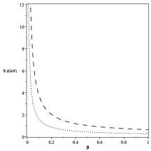
Figure 1: The dot-line (……) stands for the fundamental level of energy, $E_{0}$, and the dashed-line (- - - - -) represents the first exited energy level, $E_{1}$; both as a function of the parameter $\beta$, with $\varsigma=1.$ The mass of the quarks are taken as $m=0.336$ $MeV$ and $\lambda=0.22$ $MeV^{2}$ corn333 ; cor334 .

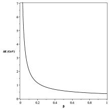
Figure 2: The difference of the levels of energy $\Delta E=E_{1}-E_{0}$ as a function of the parameter $\beta$, with $\varsigma=1.$

Wigner function for the fractional parameter for $\alpha=0.5$, and different values of $\beta$ is presented in Fig. 3. The figure compares fractional Wigner functions to the original one, which is $\alpha=\beta=1$. We observe that the peaks diminish by lowering $\beta$.

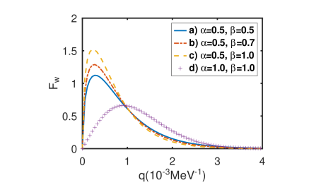
Figure 3: Comparison of fractionary Wigner functions and the non-fractionary one in the cut off of $\dfrac{p^{2}}{2m}=0$ in Eq. (26). Increasing the value of the $\dfrac{p^{2}}{2m}$ in the cut of the Wigner function will show a shift for the left, thus giving a maximum value of $p$. for the existence of the function. The original Wigner function is given when $\alpha=\beta=1$.

The curves a) to c) of Fig. 3 shows that increasing $\beta$ the peaks of Wigner functions increase. Additionally, we see that the peaks decrease to zero as $\beta$ goes to zero. Does $\beta$ functions as a fitting parameter for the fractional Wigner function of the $c\bar{c}$ meson. The curve d) is the original Wigner function without the fractional parameters for $c\bar{c}$ meson AS_1 . In Fig. 4 shows that increasing $\beta$ the distance $q$ decreases. The maximum value of $\beta$ is the best fit for the case of $\alpha=0.5$. When compared to the experimental evidence; for comparison, the experimental value for the maximum distance is $q_{0}=4.077\cdot 10^{-3}MeV^{-1}$ A_1 .

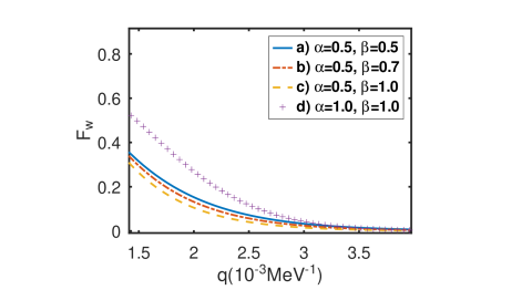
Figure 4: It is presented only a small part of Fig. 3. It is observed that the maximum distance of existence decreases with lowering $\beta$.

For the case of general Cornell potential, Eq. (1), one can linearize to get an approximation form. In the first approximation

$$V(q)=-\frac{2\sigma}{q_{0}}+\Big{(}\lambda+\frac{\sigma}{q_{0}^{2}}\Big{)}q,$$ (27)

where $a,b$ and $q_{0}$ are constants. Then the Hamiltonian is

$$(H\star)\psi=\frac{(p\star)^{2}}{2m}\psi+\Big{(}\lambda+\frac{\sigma}{q_{0}^{2}}\Big{)}(q\star)\psi=\Big{(}E+\frac{2\sigma}{q_{0}}\Big{)}\psi.$$ (28)

This equation leads to

$$(H\star)\psi=\frac{(p\star)^{2}}{2m}\psi+\lambda^{\prime}(q\star)\psi=E^{\prime}\psi,$$ (29)

It is worth noting that Eq. (29) is the same as Eq. (12) with $\lambda^{\prime}=\lambda+\dfrac{\sigma}{q_{0}^{2}}$ and $E^{\prime}=E+\frac{2\sigma}{q_{0}}$. Therefore the same analysis applies here. The energy is given by

$$E_{n}=\kappa\bigg{(}2n+\frac{3}{2}\bigg{)}-\frac{2\sigma}{q_{0}},$$ (30)

where $\kappa=\sqrt{A\eta}$ and $\eta=\frac{{\lambda^{\prime}}^{2}}{8m}$. It is noteworthy that, when $q\rightarrow 0$, in the general Cornell potential has the $q^{-1}$ that is responsible by interaction at short distances and corresponding to one gluon exchange. In addition, in Table 1 presents the theoretical results from the fractional model for $\alpha=0.5$, $\beta=1.0$, calculated from Eq.(23), and the respective experimental values. Comparisons were established only for 1S states, as our theoretical model is applicable only to such states. We didn’t include spin in our theoretical model. We noticed that there is good accuracy between the theoretical and experimental results particle , better than those obtained by other theoretical models corn333 .

Table 1: Experimental and Theoretical masses (in $MeV$) of charmonium mesons.

Meson	Fractional Cornell Potential	Experimental Data particle
$J/\Psi(1S)$	$3,1003$	$3,0969$
$\Upsilon(1S)$	$9,4818$	$9,4603$
$\eta(1S)$	$2,7992$	$2,9796$

V Final Remarks

We have studied the symplectic Schrödinger-like equation in the presence of a linear potential using the formalism of generalized fractional derivatives for non-relativistic heavy quarkonium bound state. For this purpose we have investigated the behavior of the Wigner function for the ground-state $c\overline{c}$ meson considering the symplectic quantum mechanics and the generalized fractional derivative constructed in RL_1 ; AS_1 . The Wigner function has been obtained for the charmonium state in the fractional form using the generalized fractional derivative as in Ref. B_1 , where we obtained the classical case at $\alpha=\beta=1$. To obtain an analytical solution, we analyse the case $\alpha=0.5$ . For this value of $\alpha$, it was observed that the peaks of the Wigner function is lowered by decreasing fractional parameter $\beta$, therefore, this parameter can be used as a fitting parameter. For the case of $\alpha=0.5$ the value $\beta=1$ is the best fit considering the experimental evidence. Therefore, the present analysis, seems to indicate the relevance of such a generalized fractional model based on the symplectic Schrödinger equation with linear term (Cornell potential) as far as quarkonium dynamics in phase space is concerned. To further the study of a quarkonium system within the fractional and phase space approaches, we will include a quadratic term (or correction term) at the Cornell potential and other values for the fractional parameter $\alpha$. We also intend to study spinorial systems.

Acknowledgments

This work was supported by CNPq and CAPES (Brazilian Agencies).

References

- (1) H. Mansour and A. Gamal, Adv. High Energy Phys. 2018, 7 (2018).
- (2) M. Abu-Shady, Int. J. App. Math. and Theor. Phys., 2, 16 (2016).
- (3) N. R. Soni, B. R. Joshi, R. P. Shah, H. R. Chauhan, and J. N. Pandya, Eur. Phys. J. C 78, 1 (2018).
- (4) R. Mann, An introduction to particle physics and the standard model., (CRC press 2009).
- (5) S. Gasiorowicz, Elementary particle physics., (Wiley, New York, 1966).
- (6) D. Griffiths, Introduction to elementary particles., (John Wiley & Sons, New York, 2008).
- (7) I. J. R. Aitchison and A. J. G. Hey, Gauge Theories in Particle Physics: A Practical Introduction: From Relativistic Quantum Mechanics to QED., (IOP Publishing, Bristol, 2012).
- (8) S. Weinberg, The Discovery of Subatomic Particles Revised Edition., (Cambridge University Press, Cambridge, 2003).
- (9) M. Thomson, Modern Particle Physics, (Cambridge University Press, Cambridge, 2013).
- (10) H. Mutuk, Adv. High Energy Phys. 2019, 9 (2019).
- (11) S. Koothottil, J. P. Prasanth, and V. M. Bannur, In: Proc. of the DAE Symp. on Nucl. Phys. 62, 912 (2017).
- (12) F. Tajik, Z. Sharifi, M. Eshghi, M. Hamzavi, M. Bigdeli, S. M. Ikhdair, Phys. A: Stat. Mech. and App. 535, 122497, (2019).
- (13) N. Ferkous and A. Bounames, Commun. Theor. Phys. 59, 679 (2013).
- (14) S. M. Ikhdair, Adv. High Energy Phys. 2013, 10 (2013).
- (15) A. I. Ahmadov et al, J. Phys.: Conf. Ser. 1194, 012001 (2019).
- (16) H. S. Chung, J. Lee, and D. Kang, arXiv preprint arXiv:0803.3116, (2008).
- (17) M. Abu-Shady and E. M. Khokha, Adv. high energy Phys. 2018, 7032041 (2018).
- (18) A. Vega and J. Flores, Pramana - J. Phys. 87, 73 (2016).
- (19) P. Czerski, E.P.J Web of Conf. 81, 05008 (2014).
- (20) P. Gupta and I. Mehrotra, J. Mod. Phys., 3, 1530 (2012).
- (21) E. V. B. Leite, H. Belich, and R. L. L. Vitória, Adv. High Energy Phys. 2019, 7 (2019).
- (22) G. X. A. Petronilo, R. G. G. Amorim, S. C. Ulhoa, A. F. Santos, A. E. Santana, and Faqir C. Khanna, Int. J. Mod. Phys. A, 2150121 (2021).
- (23) E. P. Inyang, E. P. Inyang, E. S. William, and E. E. Ibekwe, Jordan J. Phys. 14, 337 (2021).
- (24) I. O. Akpan, E. P. Inyang, E. P. Inyang, and E. S. William, Rev. Mex. Fís. 67, 482 (2021).
- (25) H. Dessano, R. A. S. Paiva, R. G. G. Amorim, S. C. Ulhoa, and A. E. Santana, Braz. J. Phys. 49, 715 (2019).
- (26) F. Ahmed, Eur. Phys. Lett. 133, 50002 (2021).
- (27) A. Mirjalili and M. Taki, Theor. Math. Phys. 186, 280 (2016).
- (28) T. A. Nahool, A. M. Yasser, M. Anwar, and G. A. Yahya, East Eur. J. Phys. 3, 31 (2020).
- (29) E. Omugbe, Can. J. Phys. 98, 1125 (2020).
- (30) E. M. Khoka, M. Abu-Shady, and T. A. Abdel-Karim, Int. J. Theor. App. Math. 2, 86 (2016).
- (31) E. P. Inyang, E. P. Inyang, I. O. Akpan, J. E. Ntibi, and E. S. William, Eur. J. App. Phys. 2, 6 (2020).
- (32) E. P. Inyang, E. P. Inyang, J. Karniliyus, J. E. Ntibi, and E. S. William, Eur. J. App. Phys. 3, 48 (2021).
- (33) R. R. Luz, C. S. Costa, G. X. A. Petronilo, A. E. Santana, R. G. G. Amorim, and R. A. S. Paiva, Adv. High Energy Phys., 2022, 3409776, (2022), arvix: https://arxiv.org/abs/2110.12223.
- (34) M. Abu-Shady and M. K. Kaabar, Math. Probl. Eng. 2021, 9444803, 9 (2021).
- (35) M. Abu-Shady, S. Y. Ezz-Alarab, Few-Body Syst. 62, 13 (2021).
- (36) M. Abu-Shady, Int. J. Mod. Phys. A 343, 1950201 (2019).
- (37) K. B. Oldham, J. Spanier, The Fractional Calculus (Academic Press, New York, 1974).
- (38) A. Al-Jamel, J. Int. Mod. Phys. A 34, 1950054 (2019).
- (39) M. Abu-shady, A. I. Ahmadov, H. M. Fath-Allah, V. H. Badalov, J. Theor. App. Phys. 3, 16 (2022) 10.30495/jtap.162225.
- (40) H. Karayer et al, Commun. Theor. Phys. 66, 12 (2016).
- (41) M. D. Oliveira, M. C. B. Fernandes, F. C. Khanna, A. E. Santana, and J. D. M. Vianna, Ann. Phys. (N.Y.) 312, 492 (2004).
- (42) P. Campos, M. G. R. Martins, M. C. B. Fernandes, and J. D. M. Vianna, Ann. Phys. (N.Y.) 390, 60 (2018).
- (43) P. Campos, M. G. R. Martins, and J. D. M. Vianna, Phys. Lett. A 381, 1129 (2017).
- (44) M. B. de Menezes, M. C. B. Fernandes, M. G. R. Martins, A. E. Santana, and J. D. M. Vianna, Ann. of Phys. (N.Y.) 389, 111 (2017).
- (45) M. Abu-Shady and M. K. A. Kaabar, Comp. and Math. Meth. in Med., 2022, 2138775, 5, (2022).
- (46) W. Lucha, F. F. Schöbel, Phenomenological Aspects of Nonrelativistic Potential Models, HEPHY/PUB-527, UWTh-1989-71 (1989).
- (47) C. Mena, L. F. Palhares, arXiv:1804.09564v2 [hep-ph] 25 (2018).
- (48) Particle Data Group, Phys. Lett. B 204, 1, (1988).