$S^{2}$-Transformer for Mask-Aware Hyperspectral
Image Reconstruction

Abstract

The technology of hyperspectral imaging (HSI) records the visual information upon long-range-distributed spectral wavelengths. A representative hyperspectral image acquisition procedure conducts a 3D-to-2D encoding by the coded aperture snapshot spectral imager (CASSI) and requires a software decoder for the 3D signal reconstruction. By observing this physical encoding procedure, two major challenges stand in the way of a high-fidelity reconstruction. ($i$) To obtain 2D measurements, CASSI dislocates multiple channels by disperser-titling and squeezes them onto the same spatial region, yielding an entangled data loss. ($ii$) The physical coded aperture (mask) leads to a masked data loss by selectively blocking the pixel-wise light exposure. To tackle these challenges, we propose a spatial-spectral ($S^{2}$-) Transformer network with a mask-aware learning strategy. First, we simultaneously leverage spatial and spectral attention modeling to disentangle the blended information in the 2D measurement along both two dimensions. A series of Transformer structures are systematically designed to fully investigate the spatial and spectral informative properties of the hyperspectral data. Second, the masked pixels will induce higher prediction difficulty and should be treated differently from unmasked ones. Thereby, we adaptively prioritize the loss penalty attributing to the mask structure by inferring the pixel-wise reconstruction difficulty upon the mask-encoded prediction. We theoretically discusses the distinct convergence tendencies between masked/unmasked regions of the proposed learning strategy. Extensive experiments demonstrates that the proposed method achieves superior reconstruction performance compared with state-of-the-art Transformer-based networks. Additionally, we empirically elaborate the behaviour of spatial and spectral attentions under the proposed architecture, and comprehensively examine the impact of the mask-aware learning, both of which advances the physics-driven deep network design for the HSI reconstruction. Code and pre-trained models are available at https://github.com/Jiamian-Wang/S2-transformer-HSI.

1 Introduction

The technology of hyperspectral imaging (HSI) records pixels of the scene across a wide range of spectrum. The obtained hyperspectral images enable not only high spatial resolutions, but also fine wavelength resolutions. Due to their expressiveness in both domains, hyperspectral images are widely used in applications of biomedicine, remote sensing, astronomy [1, 2, 3, 4] etc. For hyperspectral image acquisition, one of the most popular systems is the coded aperture snapshot compressive imager (CASSI) [5, 6]. It operates as an optical encoder, which compresses the hyperspectral signals into 2D measurements, and requires a software decoder for the signal retrieval [7]. Recently, how to perform high-fidelity reconstruction draws lots of attention.

From model-based algorithms [8, 9, 10, 11, 12, 13], to learning-based methods [14, 15, 16, 17, 18], existing efforts have made remarkable progress in solving the inverse problem of the CASSI-based encoding procedure. However, how to reconstruct the signal at zero-distortion still remains an open-problem, due to the sparsity of the sensing matrix upon compression [19]. Different from previous works, we propose to tackle this challenge by tracing the compressive data loss observed from the optical procedure. In light of this, two types of the data loss are presumed. (1) CASSI compresses the information of multiple wavelengths to a 2D measurement by the channel-wise entangling and addition (implemented by a disperser), which leads to the entangled data loss. (2) CASSI blocks the light with a physical binary mask for encoding, yielding the masked data loss spatially.

For the entangled data loss, we resort to exploiting the nature of hyperspectral images for a better signal compensating upon the 2D measurement. As shown in Fig. 1, hyperspectral data provides both spatial and spectral informative clues. Spatially, different wavelengths detect different patterns. Also, spatial textures among adjacent wavelengths (e.g., 498.0nm and 503.9nm in neighbor A, 614.4nm and 625.1nm in neighbor B) are highly correlated. Such a correlation diminishes among more far-between wavelengths as compared by region 1. From a spectral perspective, each hyperspectral image possesses a unique spectral distribution, indicating the specialized long-range dependencies among sampled wavelengths, e.g., Spectral Corr (short for ‘correlation’) in Fig. 1.

Bearing the above properties, popular off-the-shelf spatial/spectral Transformers [20, 14] show limitations in fully exploiting the hyperspectral data. (1) Spatial attention uses a 2D attention matrix to describe spatial contents at different channels, neglecting the inherent spectral variation within each token. While the multi-head structure empowers the representation diversity, it requires a carefully hand-crafted design. (2) Spectral attention considers the channel relationships by the attention matrix, whose dimensionality invariants to the token spatial size. This property thresholds the fine visual ingredients allocation of the attention mechanism. Furthermore, both attentions are inter-dependent, requiring a proper interaction between two dimensions.

For the masked data loss, we consider from the data uncertainty [21] perspective of view by recognizing the masked pixels with more uncertainty over unmasked ones. Existing L1 or L2 losses obscure such an optical-induced uncertainty with the inherent high-frequency texture-induced aleatoric uncertainty by treating pixels equally – as shown in Fig. 6 (b), the difficulty (uncertainty) map by MST appears a mask pattern, despite its globally impressive performance. Besides, the pixel-wise reconstruction difficulty varies to the prediction along the optimization process, which requests a dynamic schedule to properly infer the underlying uncertainty.

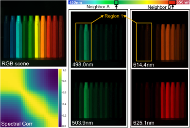
Figure 1: Hyperspectral image characteristics. Spatial correlations vary from adjacent wavelengths (e.g., neighbor A, B) to distant bands (region 1). The bottom-left correlation matrix upon multiple sampled wavelengths (i.e., 28$\times$28) defines a unique spectral distribution of a hyperspectral image. Spatial and spectral properties are inter-dependent.

In this study, we propose a spatial-spectral ($S^{2}$-) Transformer with a mask-aware learning strategy. Firstly, we present parallel spatial-spectral attention structure, based on which we reveal the distinct functionalities of both attentions in hyperspectral modeling. Secondly, we propose a mask-aware learning strategy to explicitly consider the hardware-induced pixel-wise reconstruction difficulties, which assumes that the similar spirit of [21, 22], i.e., pixels with higher “uncertainty” (regression difficulty) should be prioritized for loss penalty. Specifically, we obtain a difficulty-level cube by referring to the physically encoded signal, and then adaptively penalize the pixel-wise reconstruction weighted by this cube. We summarize the contributions as follows:

• By observing the signal optical acquisition procedure, we study two types of data loss that will impede a high-fidelity hyperspectral image retrieval, serving as the first attempt to expedite the interpretability of designing deep reconstruction networks for HSI from the physical scope.

• For the entangled data loss, we propose an $S^{2}$-Transformer by systematically investigating different self-attention structures concerning hyperspectral characteristics, based on which we empirically uncover the different functionalities of spatial and spectral attentions.

• For the masked data loss, we introduce a mask-aware learning strategy. Both the theoretical analysis and empirical evidence present the prioritization effect of the proposed schedule toward masked regions, which further boosts the reconstruction perceptually and quantitatively.

• Extensive experiments demonstrate the superior performance of the proposed method over the state-of-the-arts quantitatively and perceptually. Our observations and inductions lay the foundation for the future Transformer architecture design following the CASSI encoding.

The rest of this paper is organized as follows. Section 2 introduces the related works in detail. Section 3 develops the proposed $S^{2}$-Transformer and theoretically discusses the mask-aware learning strategy. Extensive experiments of performance, ablation studies, and visual grounded evidence are demonstrated in Section 4. Section 5 concludes this paper.

2 Related Work

Inspired by the compressed sensing (CS) theories [23, 24], a series of HSI technologies such as occlusion mask [25], spatial light modulator [26] and digital-micromirror-device [27] have also been used for hyperspectral imaging. Some other systems use multiple-shots [28], dual-channel [29, 30, 31, 32] and high-order information [33] to improve the performance. In comparison, coded aperture snapshot spectral imager (CASSI) uses a coded aperture and a prism to implement the spectral modulation, which serves as one of the most popular optical designs due to its concise setup, short acquisition time, low-cost consumption, and low-power usage [7].

CASSI plays a role of optical encoder by compressively tweaking and storing the hyperspectral signal into 2D measurements. Correspondingly, it requires software-based algorithms for the signal retrieval. Existing works tackle this ill-posed reconstruction problem from different perspectives. Previously, regularization-based optimization algorithms [11, 12, 13] adopt various priors to confine the signal space, such as sparsity [13], and total variation (TV) [34], etc. Among them, DeSCI [9] estimates the low-rank matrix structure of similar patch groups and leads to excellent performance. However, these methods generally can provide limited reconstruction performance and sometimes suffer from the unstable convergence and long running time.

Different from the regularization-based algorithms, deep unfolding methods  [17, 35, 36, 37, 38] employ the deep neural networks as denoisers in the widely-used optimization solver such as alternating direction method of multipliers (ADMM) [39]. Among them, the [35] adopts a prior network to jointly learn the local coherence and dynamic characteristics of hyperspectral data, while [40] integrates the local and non-local correlation exploitation in the learnable module. Despite the strong interpretability and end-to-end learning property of the unfolding methods, the computational complexity and efficiency degrades with more stages of CNN models introduced. Another way of combining the optimization algorithm with deep networks is the Plug-and-Play (PnP) frameworks [41, 42, 18], where pretrained deep networks are incorporated as denoisers for a better efficiency, robustness, and performance trade-off. However, pretrained deep denoisers without re-training limits the performance of the framework. Also, the proper determination of pretrained models remain underexplored.

Inspired by strong representation ability of convolutional neural networks, deep CNN model-based methods [43, 44, 35, 45] have been introduced for a high-fidelity reconstruction. Among them, $\lambda$-net [44] incorporates a generative adversarial learning framework. TSA-Net [15] firstly introduces the self-attention in both spatial and spectral domain. However, it heavily relays on the spatial locality of convolution for the down-scaled attention map calculation, leading to limited long-range relationship modeling capacity. DGSMP [29] formulates the reconstruction as a MAP problem and effectively learns the prior, achieving better performance. BIRNAT [46] adopts bidirectional RNNs for a follow-up channel retrieval, exploiting the sequential property of the hyperspectral data for the first time. Besides, HDNet [47] mainly regularizes the reconstruction in the frequency domain upon discrete Fourier transform (DFT). It performs the spatial-spectral learning with convolutional structure for a better feature extraction, but barely discloses the spatial and spectral characteristics of the hyperspectral images underlying the model design principles. More recently, Transformer architectures [48, 20] becomes an emerging option for the hyperspectral image reconstruction. Specifically, MST [14] models the long-range dependencies across different spectral channels. Besides, it creatively inserts the mask to customize the self-attention calculation. Employing spatial sparsity of the hyperspectral images, CST [16] selectively computes the self-attention within informative spatial windows and clusters semantically-similar tokens into buckets regardless the pixel spatial location, which sets the state-of-the-art performance with low complexity.

Different from the prior efforts, in this work, our proposed method is inspired by observing the physical encoding process of the CASSI. We attribute the reconstruction difficulty into two types of data loss and present the solutions respectively. For the entangled data loss, we systematically explore both spatial and spectral attentions under a unified structure. We uncover the distinct functionalities of spatial and spectral attention under the best-performed attention arrangement. For the masked data loss, we introduce a mask-aware learning strategy, which identifies among spatial regions from the data uncertainty perspective of view. The theoretical discussion for the proposed strategy is provided.

3 Method

We firstly give a preliminary knowledge of hyperspectral imaging. We also uncover the potential challenges that may set the bottleneck for the reconstruction performance. Followed by, we propose an $S^{2}$-Transformer architecture with mask-aware learning strategy as a corresponding solution.

3.1 Preliminary Knowledge

The CASSI-based hyperspectral imaging process consists of an optical encoder and a software decoder. Let $\mathbf{F}\in\mathbb{R}^{H\times W\times N_{\lambda}}$ represent the hyperspectral cube with $N_{\lambda}$ discrate wavelengths (spectral channels), $\mathbf{M}\in\mathbb{R}^{H\times W}$ denotes the physical coded aperture (mask). As shown in Fig. 2, the whole compression procedure could be simplified as two steps. CASSI firstly encodes the signal by

$$\mathbf{F}^{\prime}=\mathbf{F}\odot\mathbf{M},$$ (1)

where $\odot$ denotes a pixel-wise multiplication with broadcasting, and $\mathbf{F}^{\prime}$ denotes a “sponge” cube encoded by the mask. Note that the visual information of certain pixels will be erased according to the mask pattern, i.e., where $\mathbf{M}_{ij}$$=$$0$, or partially disrupted by the noisy mask values, i.e., $\mathbf{M}_{ij}$$\in$$(0,1)$, both of which lead to the reconstruction challenge of masked data loss. After that, the CASSI titles $\mathbf{F}^{\prime}$ by $y$-axis-shearing, specifically, $\mathbf{F}^{\prime}(u,v,n_{\lambda})\rightarrow\mathbf{F}^{\prime}(u,v+d(\lambda-\lambda^{*}),n_{\lambda})$, where $\lambda$ indicates the wavelength of the $n_{\lambda}$-th spectral channel. The $\lambda^{*}$ denotes the pre-defined anchor wavelength, and $d(\cdot)$ defines the shifting principle. We conduct a two-pixel shift for each spectral channel following [15]. CASSI finally produces the measurement $\mathbf{Y}\in\mathbb{R}^{H\times(W+d(N_{\lambda}-1))}$ by

$$\mathbf{Y}=\textstyle\sum_{n_{\lambda}=1}^{N_{\lambda}}\mathbf{F}^{\prime}(:,:,n_{\lambda})+\mathbf{\Omega},$$ (2)

where $\mathbf{\Omega}$ denotes the measurement noise. Notably, the pixel-wise addition by Eq. (2) imposes the second reconstruction challenge of entangled data loss as one needs to precisely distinguish the spatial details of a specific wavelength from another one given the single 2D measurement.

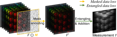
Figure 2: CASSI pipeline (best viewed in color).

From a physical encoding perspective, a high-fidelity reconstruction is largely about properly tackling the two-fold data loss. For the entangled data loss, we trace back to the nature of the hyperspectral cube, and design a spatial-spectral attention ($S^{2}$-attn) mechanism accordingly in expectation to disassemble the spectral signals out of the measurement. We systematically discuss this part in Section 3.3. In Section 3.4, we explicitly measure the pixel-wise difficulty-level owning to the masked data loss, and propose a curriculum training strategy [49, 50], mask-aware learning, without additional training cost (i.e., time, parameters) introduced.

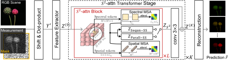
Figure 3: Overview of the spatial-spectral ($S^{2}$-) Transformer. The network takes the 2D measurement $\mathbf{Y}$ with the mask $\mathbf{M}$ as input and retrieves the hyperspectral image $\widehat{\mathbf{F}}$. It mainly contains $K$ stages, where each consists of $L$ $S^{2}$-attn blocks. Both sequential ($\mathbf{Z}_{\texttt{Sequn-SS}}$) and paralleled ($\mathbf{Z}_{\texttt{Parall-SS}}$) blocks employ spatial and spectral multi-head self-attention (MSA). We perform window partition to the embedding before MSA. Visualization takes one window in a head as an example.

3.2 Overall Architecture

The proposed spatial-spectral ($S^{2}$-) Transformer primarily builds upon the self-attention mechanism [48]. Following the merit of [51, 15, 52], we initialize the network input $\mathbf{Y}^{\prime}$$\in$$\mathbb{R}^{H\times W\times N_{\lambda}}$ by measurement $\mathbf{Y}$ via a channel-wise shift operation and a pixel-wise production with mask

$$\mathbf{Y}^{\prime}(:,:,n_{\lambda})=\mathbf{Y}(:,d(\lambda-\lambda^{*}):d(\lambda-\lambda^{*})+W)\odot\textbf{M},$$ (3)

where $\odot$ denotes a pixel-wise multiplication. The whole network is given by $\widehat{\mathbf{F}}=f(\theta;\mathbf{Y}^{\prime})$, where $\theta$ denotes the learnable parameters and $\widehat{\mathbf{F}}$ represents the reconstruction result. As shown in Fig. 3, the proposed network is composed of three parts. 1) A feature extractor by a CONV3$\times$3 layer, producing $\mathbf{Z^{(0)}}\in\mathbb{R}^{H\times W\times C}$. Let $C$ denote the number of embedding channels, which should be large enough to provide the redundancy for the spectrum correlation exploitation. 2) A reconstruction head employs a CONV3$\times$3 layer, which maps the embedded space to the hyperspectral domain. 3) $K$ consecutive $S^{2}$-attn Transformer stages. Each stage is characterized by a residual structure. Concretely, both $L$ concatenated $S^{2}$-attn blocks and one CONV3$\times$3 layer are governed by an identity connection in a stage. Let $\mathbf{Z}^{(k)}\in\mathbb{R}^{H\times W\times C}$ denote the output of the $k$-th stage, $1\leq k\leq K$. The feed-forward function $f_{\texttt{S}}(\cdot)$ of the stage is

$$\mathbf{Z}^{(k)}=f_{\texttt{S}}(\mathbf{Z}^{(k-1)})=\mathbf{Z}^{(k-1)}+\texttt{CONV}(f_{\texttt{L}}(\mathbf{Z}^{(k-1)})),$$ (4)

where $\mathbf{Z}^{(k-1)}$ denotes the output embedding of the previous stage. In each stage, we further expand the mapping of $L$ consecutive blocks $f_{\texttt{L}}(\cdot)$$=$$f_{\texttt{B}}(...f_{\texttt{B}}(\cdot)...)$ in Eq. (4) by

$$\mathbf{Z}^{(k-1,L)} =f_{\texttt{L}}(\mathbf{Z}^{(k-1,0)}),$$ (5)

$$\mathbf{Z}^{(k-1,l)} =f_{\texttt{B}}(\mathbf{Z}^{(k-1,l-1)}),$$

where $l=\{1,...,L\}$ and $f_{\texttt{B}}(\cdot)$ expresses the mapping of a single $S^{2}$-attn block. Notably, to avoid the quadratic complexity in the traditional self-attention calculation [48], we perform the window partition following [53, 54] toward the feature embedding for all types of attention mechanisms.

Hyperspectral images inherently provide spatially and spectrally informative clues for the signal compensating upon the 2D measurement (see Fig. 1). Also, the spatial and spectral characteristics are inter-dependent, which contributes to the 3D signal retrieval hindered by the entangled data loss. This study will systematically exploit the underlying cues by introducing different types of $S^{2}$-attn blocks.

3.3 Spatial & Spectral Attention Blocks

In this section, we give a brief introduction toward both spatial and spectral attentions. We uncover their advantages and potential limitations underlying hyperspectral characteristics, respectively. Furthermore, we propose hybrid spatial-spectral attention structures and systematically discuss their behaviours toward the hyperspectral data modeling.

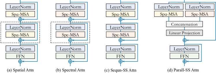
Figure 4: Different spatial-spectral ($S^{2}$-) attention blocks, which are readily wrapped by off-the-shelf components, i.e., layer normalization (LN), and multi-head self-attention (MSA). Single-typed attentions (a, b) are enhanced by additional LN-MSA (in dashed boxes) for a comparable complexity. All the attention blocks takes the feature embedding upon the window partition.

Spatial Attention. Since proposed by [48] and developed in [20], the frequently-used spatial attention (Spa) has been evolved with key components of multi-head self-attention (MSA), layer normalization (LN) [55], and feed-forward network (FFN). Given the input of the size $H$$\times W$$\times C$, the attention module partitions it into $\frac{HW}{M^{2}}$ windows, where $M$ is the window size. We adopt the multi-head self attention (MSA) module for the attention computation. Let $T$ be the number of heads. Each head in MSA is allocated with $C_{h}$$=$$\lfloor\frac{C}{T}\rfloor$ channels. For the annotation simplicity, we demonstrate the computation within a window for each head by feeding the attention modules with the input feature embedding $\mathbf{Z}_{\texttt{in}}\in\mathbb{R}^{M^{2}\times C_{h}}$ accordingly. All the other windows among different heads follow the same computational procedure. As shown in Fig. 4 (a), the mapping is conducted by

$$\mathbf{Z}_{\texttt{Spa}} =f_{\texttt{Spa-MSA}}(\texttt{LN}(\mathbf{Z}_{\texttt{in}}))+\mathbf{Z}_{\texttt{in}},$$ (6)

$$\mathbf{Z}_{\texttt{out}} =f_{\texttt{FFN}}(\texttt{LN}(\mathbf{Z}_{\texttt{Spa}}))+\mathbf{Z}_{\texttt{Spa}},$$

where $f_{\texttt{FFN}}(\cdot)$ is instantiated by a Linear-GELU-Linear-GELU structure, and $f_{\texttt{Spa-MSA}}(\cdot)$ denotes a MSA module, yielding $\mathbf{Z}_{\texttt{Spa}}$. The $\mathbf{Z}_{\texttt{out}}$ denotes the final output of the spatial attention block. We adopt $\mathbf{Q}$, $\mathbf{K}$, and $\mathbf{V}\in\mathbb{R}^{M^{2}\times C_{h}}$ to represent the query, key, and value, and compute them with the feature embedding $\mathbf{Z}_{\texttt{in}}$ and a linear projection by

$$\mathbf{K}=\mathbf{W}^{\mathbf{K}}\mathbf{Z}_{\texttt{in}},~{}\mathbf{Q}=\mathbf{W}^{\mathbf{Q}}\mathbf{Z}_{\texttt{in}},~{}\mathbf{V}=\mathbf{W}^{\mathbf{V}}\mathbf{Z}_{\texttt{in}},$$ (7)

where $\mathbf{W}^{\mathbf{K}}$, $\mathbf{W}^{\mathbf{Q}}$, and $\mathbf{W}^{\mathbf{V}}$ are learnable parameters. The output of spatial attention $\mathbf{Z}_{\texttt{Spa}}$ is given as

$$\mathbf{A}_{\texttt{Spa}} =\texttt{softmax}(\mathbf{K}\mathbf{Q}^{T}/\beta+\mathbf{B}),$$ (8)

$$\mathbf{Z}_{\texttt{Spa}} =\mathbf{A}_{\texttt{Spa}}\mathbf{V},$$

where $\beta$ is a learnable scaling factor for the overlarge values, initialized as $\sqrt{C_{h}}$, $\mathbf{B}$ represents a learnable position bias matrix following [56, 57], and $\mathbf{A}_{\texttt{Spa}}$$\in$$\mathbb{R}^{M^{2}\times M^{2}}$ stands for self-attention matrix in a partitioned window. The outputs of $T$ heads will be concatenated afterward.

Given the spatial tokens of the size $1$$\times$$1$$\times C_{h}$, the spatial attention benefits the reconstruction by 1) taking well advantage of semantic clues of each pixel, 2) enabling interactions among neighbored channels within each head, which meets with the nature that spectral-adjacent contents are highly correlated (neighbor A, B in Fig. 1). However, it shows limitations in describing the spectral variations of each token.

Spectral Attention. We leverage the self-attention in spectral domain (Spe) after the window partition. The attention module shares a similar architecture to Eq. (6), but differs in multi-head self-attention (MSA) computation, i.e., $f_{\texttt{Spe-MSA}}(\cdot)$, for the spectral dependency modeling. We compute query, key, and value with Eq. (7) and the spectral attention in each window is computed by

$$\mathbf{A}_{\texttt{Spe}} =\texttt{softmax}(\mathbf{K}^{T}\mathbf{Q}/\beta+\mathbf{B}),$$ (9)

$$\mathbf{Z}_{\texttt{Spe}} =\mathbf{V}\mathbf{A}_{\texttt{Spe}},$$

where $\mathbf{Z}_{\texttt{Spe}}\in\mathbb{R}^{M^{2}\times C_{h}}$ refers to the output feature embedding of $f_{\texttt{Spe-MSA}}(\cdot)$ and $\mathbf{A}_{\texttt{Spe}}$ $\in\mathbb{R}^{C_{h}\times C_{h}}$ stands for the self-attention matrix of the partitioned cube in each head. We scale the matrix multiplication by a learnable scalar $\beta$ and add $\mathbf{B}$ as a relative position bias matrix [58].

Computed with the spectral token of the size $M$$\times M$$\times 1$, the dimensionality of the spectral attention matrix $\mathbf{A}_{\texttt{Spe}}$ differs from the $\mathbf{A}_{\texttt{Spa}}$ of the size $M^{2}\times M^{2}$. By integrally considers the pixels in a channel, the spectral attention can better abstract the inherent spectrum principle underlying discrete wavelengths. However, $\mathbf{A}_{\texttt{Spe}}$ is of $C_{h}\times C_{h}$, regardless of the token spatial size, i.e., $M\times M$. Such a resolution-agnostic property impedes the abstraction ability of the attention when visual detail increases, but instead only allows limited visual clues abstraction for the channel-wise modeling.

Considering the limitations of both attention types, it would be inadequate to solely employ either one for a high-fidelity reconstruction. Thereby, we provide two types of hybrid structure, which not only exploit two-fold advantages, but also explore the spatial-spectral inter-dependencies.

Sequential Spa-Spe Attention. We perform sequential attention (Sequn-SS) by cascading the $f_{\texttt{Spa-MSA}}(\cdot)$, $f_{\texttt{Spe-MSA}}(\cdot)$, and the feed-forword network $f_{\texttt{FFN}}(\cdot)$. As shown in Fig. 4 (c), the feed-forward pass upon the feature embedding $\mathbf{Z}_{\texttt{in}}$ is

$$\mathbf{Z}_{\texttt{Spe}}=f_{\texttt{Spe-MSA}}(\texttt{LN}(\mathbf{Z}_{\texttt{in}}))+\mathbf{Z}_{\texttt{in}},$$ (10)

$$\mathbf{Z}_{\texttt{Spa}}=f_{\texttt{Spa-MSA}}(\texttt{LN}(\mathbf{Z}_{\texttt{Spe}}))+\mathbf{Z}_{\texttt{Spe}},$$

$$\mathbf{Z}_{\texttt{Sequn-SS}}=f_{\texttt{FFN}}(\texttt{LN}(\mathbf{Z}_{\texttt{Spa}}))+\mathbf{Z}_{\texttt{Spa}},$$

where $f_{\texttt{Spa-MSA}}(\cdot)$ and $f_{\texttt{Spe-MSA}}(\cdot)$ are given by Eq. (8) and Eq. (9), respectively. The Sequn-SS explores the data correlations from spatial and spectral perspectives, and allows interaction between both attention mechanisms. However, the behaviors of these two attention types are highly interrelated and either one lacks independence. Besides, we notice the potential superiority of Sequn-SS might attribute to a large model size and higher complexity in comparison to previous attention block types under the same optimization setting. Thus, we empower the aforementioned spatial and spectral attention block designs with additional MSA-LN modules for a comparable model size and complexity, as shown by the dashed boxes in Fig. 4 (a, b).

Paralleled Spa-Spe Attention. Besides the Sequn-SS, concurrently conducting spatial and spectral attention (Parall-SS) is another hybrid schema. The outputs of both attentions will be combined in a learnable mode. As shown in Fig. 4 (d), given the feature embedding $\mathbf{Z}_{\texttt{in}}$, we have

$$\mathbf{Z}_{\texttt{cat}}=\mathbf{W}^{\texttt{cat}}[f_{\texttt{Spe-MSA}}(\texttt{LN}(\mathbf{Z}_{\texttt{in}})),f_{\texttt{Spe-MSA}}(\texttt{LN}(\mathbf{Z}_{\texttt{in}}))]+\mathbf{Z}_{\texttt{in}},$$ (11)

$$\mathbf{Z}_{\texttt{Parall-SS}}=f_{\texttt{FFN}}(\texttt{LN}(\mathbf{Z}_{\texttt{cat}}))+\mathbf{Z}_{\texttt{cat}},$$

where $[\cdot]$ denotes the concatenation and $\mathbf{W}^{\texttt{cat}}$ performs the linear projection. The underlying advantages of Parall-SS are both spatial and spectral attentions take effect upon the same input, during which their mutual interference existing in Sequn-SS is minimized. Plus, the learnable combination is more expressive in feature fusion. As a result, the proposed Parall-SS enjoys a structural superiority with negligible increase in parameters, in comparison to the other structures.

In summary, this section discusses the fors and againsts for spatial/spectral attentions adapting to the hyperspectral characterises, based on which we further propose two block designs with sequential and paralleled integration schema. By comparison, the paralleled fusion empirically allows a better modeling ability (see Section 4.3 for more analysis).

3.4 Mask-aware Learning

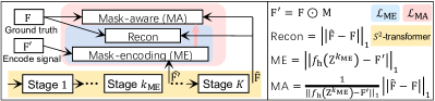
Figure 5: Mask-aware learning pipeline. We start with the mask-encoding loss ($\mathcal{L}_{\texttt{ME}}$) to estimate the encoded/complete signals. Then the mask-aware loss ($\mathcal{L}_{\texttt{MA}}$) is adopted. The mask-encoding (ME) induces the mask-aware (MA) term.

Previous works have well explored different types of learning objectives for the HSI reconstruction, e.g., $\mathcal{L}_{1}$ loss [29], RMSE [15], Spectrum Constancy [14], and perceptual loss [59], etc. By taking advantage of the semantic representations or spectral correlations, they enable promising texture retrieval and perceptual quality. However, there still exist content-irrelevant artifacts in predictions and unexpected reconstruction difficulty in smooth areas (compared by (a) and (b) in Fig. 6), as existing learning objectives attribute the reconstruction difficulty to the uncertainty upon inherent high-frequency textures, but overlook the mask-induced uncertainty. Therefore, masked and unmasked pixels are currently treated equally. From a physical perspective of view, mask encoding procedure yields the spatial data loss. Corresponding pixels should be predicted with higher uncertainty, while the unmasked regions potentially allow an easier retrieval with higher confidence.

Following this intuition, we propose a novel mask-aware learning strategy as shown in the Fig. 5. The main idea is to firstly distinguish between the masked and unmasked regions, implemented by fitting the encoded signal as $\mathbf{F}^{\prime}=\mathbf{F}\odot\mathbf{M}$. Then we adaptively emphasize masked regions with a relatively higher loss penalty. The penalization degree is determined by referring to the latest reconstruction difficulty of $\mathbf{F}^{\prime}$ throughout the training. To achieve this goal, we first pre-train the model with a mask-encoding loss ($\mathcal{L}_{\texttt{ME}}$) by

$$\mathcal{L}_{\texttt{ME}}=\alpha\underbrace{||f_{h}(\mathbf{Z}^{k_{\texttt{ME}}})-\mathbf{F}^{\prime}||_{1}}_{\rm\texttt{ME}}+\underbrace{||\widehat{\mathbf{F}}-\mathbf{F}||_{1}}_{\rm\texttt{Recon}},$$ (12)

where the mask-encoding (ME) term explores the pixel-wise reconstruction difficulty relative to the encoded signal $\mathbf{F}^{\prime}$ with early $S^{2}$-attn stages, i.e., the first $k_{\texttt{ME}}$ stages ($k_{\texttt{ME}}<K$). The $f_{h}(\cdot)$ is implemented by an LN-CONV structure. Meanwhile, we keep the original reconstruction term (Recon) to train the late blocks and stabilize the training. We use $\alpha$ to balance these two terms. In Fig. 6 (c), we visualize the estimation of the encoded signal, which is corrupted from a mask pattern as expected. By inferring from this signal, we propose a mask-aware (MA) term by taking advantage of the ME term, leading to the mask-aware loss ($\mathcal{L_{\texttt{MA}}}$) as

$$\mathcal{L}_{\texttt{MA}}=\mathcal{L_{\texttt{ME}}}+\underbrace{\dfrac{\beta}{||f_{h}(\mathbf{Z}^{k_{\texttt{ME}}})-\mathbf{F}^{\prime}||_{1}}||\widehat{\mathbf{F}}-\mathbf{F}||_{1}}_{\texttt{MA}},$$ (13)

where we attenuate the $\alpha$ inside $\mathcal{L_{\texttt{ME}}}$ after pre-training and emphasize the masked areas by determining a $\beta$ value. Note that, the ME term serves as the weight of the MA term. In the following, we will theoretically discuss the impact of the proposed mask-aware loss to the unmasked pixels and reveal a prioritization effect on the masked pixels.

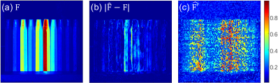
Figure 6: Visual evidence underlying mask-aware learning. (a) Reference. (b) Reconstruction difficulty by the recent method, MST [14]. (c) Estimation of encoded signal with mask-encoding loss $\mathcal{L}_{\texttt{ME}}$. We select 2D spectral channels from $\mathbf{F}$,$|\widehat{\mathbf{F}}$$-$$\mathbf{F}|$, and $\widehat{\mathbf{F}}^{\prime}$$\in$$\mathbb{R}^{H\times W\times N_{\lambda}}$ for visualization in (a$\sim$c).

On one hand, we consider a very small spatial region of the real mask so that we always have $\mathbf{M}_{ij}$$\rightarrow$$1$. Without loss of generality, we accordingly consider a feature map of $\mathbf{F}$ to simplify the notations, yet the result can be easily extended to 3D feature maps. Correspondingly, we have $\mathbf{F}_{ij}\in[0,1]$ and the encoded signal wherein $\mathbf{F}^{\prime}_{ij}$$=$$\mathbf{M}_{ij}\odot\mathbf{F}_{ij}$. Since the $\widehat{\mathbf{F}}$ overrides the embedding representation underlying $f_{h}(\mathbf{Z}^{k_{\texttt{ME}}})$, we simplify their relationship as $\widehat{\mathbf{F}}$$=$$\tau(f_{h}(\mathbf{Z}^{k_{\texttt{ME}}}))$, where $\tau(\cdot)$ represents the cascaded $S^{2}$-attn stages. Considering their residual structures, we have $\tau(\mathbf{t})$$=$$g(\mathbf{t})+\mathbf{t}$ by simplifying $f_{h}(\mathbf{Z}^{k_{\texttt{ME}}})$ as $\mathbf{t}$. The mask-aware loss $\mathcal{L}_{\texttt{MA}}$ can be rewritten as

$$\mathcal{L}_{\texttt{MA}}=\mathcal{L_{\texttt{ME}}}+\dfrac{\beta||g(\mathbf{t})+\mathbf{t}-\mathbf{F}||_{1}}{||\mathbf{t}-\mathbf{M}\odot\mathbf{F}||_{1}},\quad\mathbf{t}=f_{h}(\mathbf{Z}^{k_{\texttt{ME}}}),$$ (14)

where $g(\mathbf{t})$ represents the residual mapping and $\mathbf{t}$ is produced by the identity mapping. In the following, we finalize the induction of $\mathcal{L}_{\texttt{MA}}$ with Eq. (14) by providing an assumption and drawing a corollary.

Assumption 1.

Given a network $g_{\phi}(x)$ with non-negative input, there exists a small value $\epsilon$ upper-bounds the network output, i.e., $g_{\phi}(x)\leq\epsilon,x>0,\epsilon\rightarrow 0+$, in a small spatial region.

TABLE I: PSNR (dB) values by different methods on the benchmark simulation dataset.

Methods	Scene1	Scene2	Scene3	Scene4	Scene5	Scene6	Scene7	Scene8	Scene9	Scene10	Avg.
GAP-TV [34]	26.82	22.89	26.31	30.65	23.64	21.85	23.76	21.98	22.63	23.10	24.36
DeSCI [9]	27.13	23.04	26.62	34.96	23.94	22.38	24.45	22.03	24.56	23.59	25.27
TSA-Net [15]	32.03	31.00	32.25	39.19	29.39	31.44	30.32	29.35	30.01	29.59	31.46
DGSMP [29]	33.26	32.09	33.06	40.54	28.86	33.08	30.74	31.55	31.66	31.44	32.63
SRN [52]	34.96	35.46	36.18	41.60	32.70	34.70	33.83	32.88	35.09	32.31	35.07
HDNet [47]	35.14	35.67	36.03	42.30	32.69	34.50	33.67	32.48	34.89	32.38	34.97
MST [14]	35.40	35.87	36.51	42.27	32.77	34.80	33.66	32.67	35.39	32.50	35.18
CST [16]	35.89	36.82	38.20	42.38	33.16	35.71	34.87	34.30	36.44	33.03	36.08
$S^{2}$-Transformer	36.17	37.57	37.29	42.96	34.40	36.44	35.41	34.50	36.54	33.57	36.48

TABLE II: SSIM values by different methods on the benchmark simulation dataset.

Methods	Scene1	Scene2	Scene3	Scene4	Scene5	Scene6	Scene7	Scene8	Scene9	Scene10	Avg.
GAP-TV [34]	0.7544	0.6103	0.8024	0.8522	0.7033	0.6625	0.6881	0.6547	0.6815	0.5839	0.6993
DeSCI [9]	0.7479	0.6198	0.8182	0.8966	0.7057	0.6834	0.7433	0.6725	0.7320	0.5874	0.7207
TSA-Net [15]	0.8920	0.8583	0.9145	0.9528	0.8835	0.9076	0.8782	0.8884	0.8901	0.8740	0.8939
DGSMP [29]	0.9152	0.8977	0.9251	0.9636	0.8820	0.9372	0.8860	0.9234	0.9110	0.9247	0.9166
SRN [52]	0.9345	0.9373	0.9476	0.9703	0.9444	0.9512	0.9241	0.9443	0.9414	0.9348	0.9430
HDNet [47]	0.9352	0.9404	0.9434	0.9694	0.9460	0.9518	0.9263	0.9406	0.9415	0.9365	0.9431
MST [14]	0.9405	0.9440	0.9525	0.9734	0.9471	0.9553	0.9254	0.9479	0.9491	0.9408	0.9476
CST [16]	0.9494	0.9546	0.9623	0.9752	0.9544	0.9631	0.9451	0.9608	0.9566	0.9450	0.9566
$S^{2}$-Transformer	0.9490	0.9582	0.9567	0.9754	0.9596	0.9654	0.9461	0.9625	0.9592	0.9517	0.9584

Corollary 1.

With adequate iterations of stochastic gradient descent and a proper optimization schedule, the MA term could converge to $\sum_{ij}\pm\nabla_{\mathbf{t}_{ij}}|g(\mathbf{M}_{ij}\mathbf{F}_{ij})+\mathbf{t}_{ij}-\mathbf{F}_{ij}|$.

Proof.

We consider the situation where mask-encoding loss ($\mathcal{L}_{\texttt{ME}}$) yields a good approximation of encoded signal $\widehat{\mathbf{F}}$, where $\mathbf{t}_{ij}\rightarrow\mathbf{M}_{ij}\mathbf{F}_{ij}$. According to Eq. (14), the MA becomes

$$|g(\mathbf{t}_{ij})+\mathbf{t}_{ij}-\mathbf{F}_{ij}|\rightarrow|g(\mathbf{M}_{ij}\mathbf{F}_{ij})-(1-\mathbf{M}_{ij})\mathbf{F}_{ij}|.$$

According to Assumption 1, the residual $g(\mathbf{M}_{ij}\mathbf{F}_{ij})$ learns a small value bounded by $\epsilon$ with input $\mathbf{M}_{ij}\mathbf{F}_{ij}>0$, i.e., $g(\mathbf{M}_{ij}\mathbf{F}_{ij})\rightarrow 0$ upon enough SGD steps. Thereby, we can find

$$|g(\mathbf{M}_{ij}\mathbf{F}_{ij})-(1-\mathbf{M}_{ij})\mathbf{F}_{ij}|\rightarrow 0,$$

where the term $(1-\mathbf{M}_{ij})\mathbf{F}_{ij}$ is omitted with $\mathbf{M}_{ij}\rightarrow 1$ in the small spatial region. Accordingly, we have the numerator

$$\sum_{ij}|g(\mathbf{M}_{ij}\mathbf{F}_{ij})-(1-\mathbf{M}_{ij})\mathbf{F}_{ij}|\rightarrow 0.$$

Similarly, let $\mathbf{t}_{ij}\rightarrow\mathbf{M}_{ij}\mathbf{F}_{ij}$, the denominator becomes

$$\sum_{ij}|\mathbf{t}_{ij}-\mathbf{M}_{ij}\mathbf{F}_{ij}|\rightarrow 0.$$

Based on the previous induction, we find the indeterminacy form of both numerator and the denominator under the condition of $\mathbf{t}_{ij}\rightarrow\mathbf{M}_{ij}\mathbf{F}_{ij}$. Notably, both numerator and the denominator are differentiable on an open interval of $\mathbf{t}_{ij}$ except at $\mathbf{M}_{ij}\mathbf{F}_{ij}$, in which the denominator enables a non-zero derivation, i.e., $\sum_{ij}\nabla_{\mathbf{t}_{ij}}|\mathbf{t}_{ij}-\mathbf{M}_{ij}\mathbf{F}_{ij}|\neq 0$ for all $\mathbf{t}_{ij}$ in an open interval with $\mathbf{t}_{ij}\neq\mathbf{M}_{ij}\mathbf{F}_{ij}$. Based on these conditions, we then exploit the convergence of the MA term upon Bernoulli’s rule

$$\lim\limits_{\mathbf{t}_{ij}\to\mathbf{M}_{ij}\mathbf{F}_{ij}}\dfrac{\sum_{ij}|g(\mathbf{t}_{ij})+\mathbf{t}_{ij}-\mathbf{F}_{ij}|}{\sum_{ij}|\mathbf{t}_{ij}-\mathbf{M}_{ij}\mathbf{F}_{ij}|}$$ (15)

$$= \lim\limits_{\mathbf{t}_{ij}\to\mathbf{M}_{ij}\mathbf{F}_{ij}}\dfrac{\sum_{ij}\nabla_{\mathbf{t}_{ij}}|g(\mathbf{t}_{ij})+\mathbf{t}_{ij}-\mathbf{F}_{ij}|}{\sum_{ij}\nabla_{\mathbf{t}_{ij}}|\mathbf{t}_{ij}-\mathbf{M}_{ij}\mathbf{F}_{ij}|}$$

$$= \sum_{ij}\pm\nabla_{\mathbf{t}_{ij}}|g(\mathbf{M}_{ij}\mathbf{F}_{ij})+\mathbf{t}_{ij}-\mathbf{F}_{ij}|,$$

where $\nabla_{\mathbf{t}_{ij}}|\mathbf{t}_{ij}-\mathbf{M}_{ij}\mathbf{F}_{ij}|=\pm 1$ adapting to the value of $\mathbf{t}_{ij}$. Thus, we complete the proof. ∎

Remark. Corollary 1 uncovers a constant convergence tendency of the proposed MA term within a small spatial regions by satisfying the Bernulli’s rule. Therefore, the $\mathcal{L}_{\texttt{MA}}$ becomes

$$\mathcal{L}_{\texttt{MA}}= \alpha||f_{h}(\mathbf{Z}^{k_{\texttt{ME}}})-\mathbf{F}^{\prime}||_{1}+||\widehat{\mathbf{F}}-\mathbf{F}||_{1}$$

$$+\sum_{ij}\pm\nabla_{\mathbf{t}_{ij}}|g(\mathbf{M}_{ij}\mathbf{F}_{ij})+\mathbf{t}_{ij}-\mathbf{F}_{ij}|,$$

which indicates that the proposed MA term will not penalize the unmasked pixels, i.e., $\mathbf{M}_{ij}\rightarrow 1$. On the other hand, given a real mask value $\mathbf{M}_{ij}\rightarrow 0$ in a small spatial region and ground truth pixel value $\mathbf{F}_{ij}\in[0,1]$, we have encoded signal $\mathbf{F}^{\prime}_{ij}\rightarrow 0$. The mask-aware loss could be simplified as

$$\mathcal{L}_{\texttt{MA}}=||\widehat{\mathbf{F}}-\mathbf{F}||_{1}+\alpha||f_{h}(\mathbf{Z}^{k_{\texttt{ME}}})||_{1}+\dfrac{\beta\sum_{ij}|\widehat{\mathbf{F}}_{ij}-\mathbf{F}_{ij}|}{\sum_{ij}|f_{h}(\mathbf{Z}^{k_{\texttt{ME}}}_{ij})|},$$

where ME, MA, and Recon take effect for minimizing the overall learning objective of $\mathcal{L}_{\texttt{MA}}$. Notably, a smaller $||f_{h}(\mathbf{Z}^{k_{\texttt{ME}}}_{ij})||_{1}$ yields a larger weight of $\tfrac{\beta}{||f_{h}(\mathbf{Z}^{k_{\texttt{ME}}}_{ij})||_{1}}$. The $\sum_{ij}|\widehat{\mathbf{F}}_{ij}-\mathbf{F}_{ij}|$ needs to be further minimized to compensate for the MA value amplification. Therefore, all of the underlying masked pixels are prioritized during the reconstruction.

In summary, we theoretically present the effectiveness of the proposed mask-aware learning strategy. It adaptively enhance the reconstruction penalty for the masked pixels, while equally retrieves the unmasked pixels without discrimination, under mild conditions. Note that the mask-encoding term facilitates the mask-aware term in $\mathcal{L}_{\texttt{MA}}$, thus the pre-training upon $\mathcal{L}_{\texttt{ME}}$ is necessary for the proposed strategy.

4 Experiment

We do extensive experiments for the proposed method. Specifically, Section 4.1 introduces the experimental settings. Section 4.2 quantitatively and perceptually present the reconstruction performance on both simulation and real data. In Section 4.3, we discuss the proposed $S^{2}$-attn blocks and reason the superiority of the Parall-SS version by exploiting the underlying interpretability. In Section 4.4, we empirically analysis the mask-aware learning strategy.

4.1 Experimental Settings

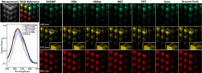
Figure 7: Reconstruction results for a simulation data. Five state-of-the-art methods and the proposed method (second to the right) are presented on 3 out of 28 wavelengths. The RGB reference is shown to demonstrate the color (top-left). The density-vs-wavelength curves (bottom-left) corresponding to the chosen patch (patch a) demonstrates the spectral fidelity.

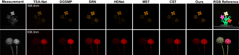
Figure 8: Reconstruction results on real-captured measurements. The proposed method retrieves more contents (e.g., the smallest hole at center of the yellow flower in top row) Zoom in for a better visualization.

Dataset. Following previous methods [15, 14, 16], we use the same dataset setting for network training and evaluation. Specifically, we adopt the CAVE [60] database for training, which provides 32 scenes with 512$\times$512 resolution and 400nm$\sim$700nm range of wavelength. The training samples are randomly cropped into 256$\times$256 patches for data augmentation. The total 28 spectral channels are determined by spectral interpolation. The testing dataset is composed of ten 256$\times$256$\times$28 hyperspectral images from the KAIST [61] dataset. In simulation, we treat the 3D hyperspectral images as ground truths and compute the 2D measurements following Eq. (1) and Eq. (2). For the real hyperspectral image acquisition, we feed the 660$\times$714 real-captured measurements by [15] into the pre-trained model, generating the 660$\times$660$\times$28 hyperspectral images accordingly. We inject the Gaussian noise to the measurements during training to simulate the real measurement noise $\mathbf{\Omega}$ in the collected data.

Implementation Details. The proposed $S^{2}$-Transformer contains $K$=4 stages, where each consists of $L$=6 $S^{2}$-attn blocks for a high-fidelity reconstruction performance. We let the number of embedding channels $C$ to be 60 and split them into $T$=6 heads in each $S^{2}$-attn block. We leverage window partitions to the feature embedding (i.e., window size $M$$=$$8$) and conduct the cyclic shifting following [54]. The model is trained for 300 epochs with Adam optimizer [62] ($\beta_{1}$=0.9, $\beta_{2}$=0.999). We set the batch size as 4. The initial learning rate is $4\times$$10^{-4}$ and halved every 50 epochs. Notably, the total amount of training epochs remains the same when employing the proposed mask-aware learning strategy. Specifically, the model is firstly pre-trained with $\mathcal{L}_{\texttt{ME}}$ for 150 epochs to get a promising approximation of the encoded signal $\widehat{\mathbf{F}}^{\prime}$. Then we train the whole model with $\mathcal{L}_{\texttt{MA}}$ for the other 150 epochs. The mask-encoding (ME) weight $\alpha$ is set as 1.5 in $\mathcal{L}_{\texttt{ME}}$ and then attenuated to 1.0 in $\mathcal{L}_{\texttt{MA}}$, and mask-aware term (MA) is weighted by $\beta$$=$$10$. We employ first half of the network to approximate the encoded signal, i.e., $k_{\texttt{ME}}$$=$$2$. Our experiments are conducted on NVIDIA RTX 3090 GPUs.

Compared Methods. We compare with eight state-of-the-art methods. Among them, DeSCI [9], and GAP-TV [34] are model-based algorithms. The CNN-based methods include TSA-Net [15], SRN [52], DGSMP [29], HDNet [47], MST [14], and CST [16], in which MST and CST are recent Transformer-based network designs. Notably, we test and report the best performance of compared methods based on their open-sourced pre-trained models. The SRN is re-trained with the same training dataset as other methods for a fair comparison. Besides, we choose the best-performed variants of the compared methods, i.e., SRN(v1), MST-L, and CST-L-Plus. For the simulation experiment, we conduct the quantitative comparison with the full-reference image quality assessment metrics, PSNR and SSIM [63]. For the real data evaluation, we adopt the no-reference image quality assessment metric, Naturalness Image Quality Evaluator (NIQE) [64] due to the inaccessibility of the ground truth.

4.2 HSI Reconstruction Performance

AA \begin{overpic}[width=125.3168pt]{white.pdf} \put(7.0,5.0){\Huge blk 22/chl 31} \end{overpic} \begin{overpic}[width=125.3168pt]{white.pdf} \put(7.0,5.0){\Huge blk 22/chl 19} \end{overpic} \begin{overpic}[width=125.3168pt]{white.pdf} \put(10.0,5.0){\Huge blk 24/chl 4} \end{overpic} \begin{overpic}[width=125.3168pt]{white} \put(7.0,5.0){\Huge blk 23/chl 29} \end{overpic} \begin{overpic}[width=125.3168pt]{white.pdf} \put(5.0,5.0){\Huge blk 23/chl 14} \end{overpic} \begin{overpic}[width=125.3168pt]{white.pdf} \put(8.0,5.0){\Huge blk 21/chl 3} \end{overpic} \begin{overpic}[width=125.3168pt]{white.pdf} \put(3.0,5.0){\Huge blk 23/chl 20} \end{overpic} \begin{overpic}[width=125.3168pt]{white.pdf} \put(3.0,5.0){\Huge blk 23/chl 20} \end{overpic} Spe-MSA \begin{overpic}[width=125.3168pt]{parallCatSS_featuremap_simu1_blk22_chl31_spemap.pdf} \put(5.0,5.0){} \end{overpic} \begin{overpic}[width=125.3168pt]{parallCatSS_featuremap_simu2_blk22_chl19_spemap.pdf} \put(5.0,5.0){} \end{overpic} \begin{overpic}[width=125.3168pt]{parallCatSS_featuremap_simu3_blk24_chl4_spemap.pdf} \put(5.0,5.0){} \end{overpic} \begin{overpic}[width=125.3168pt]{parallCatSS_featuremap_simu4_blk23_chl29_spemap} \put(5.0,5.0){} \end{overpic} \begin{overpic}[width=125.3168pt]{parallCatSS_featuremap_simu6_blk23_chl14_spemap.pdf} \put(5.0,5.0){} \end{overpic} \begin{overpic}[width=125.3168pt]{parallCatSS_featuremap_simu7_blk21_chl3_spemap.pdf} \put(5.0,5.0){} \end{overpic} \begin{overpic}[width=125.3168pt]{parallCatSS_featuremap_simu8_blk23_chl20_spemap.pdf} \put(5.0,5.0){} \end{overpic} \begin{overpic}[width=125.3168pt]{parallCatSS_featuremap_simu10_blk23_chl20_spemap.pdf} \put(5.0,5.0){} \end{overpic} Spa-MSA \begin{overpic}[width=125.3168pt]{parallCatSS_featuremap_simu1_blk22_chl31_spamap.pdf} \put(5.0,5.0){} \end{overpic} \begin{overpic}[width=125.3168pt]{parallCatSS_featuremap_simu2_blk22_chl19_spamap.pdf} \put(5.0,5.0){} \end{overpic} \begin{overpic}[width=125.3168pt]{parallCatSS_featuremap_simu3_blk24_chl4_spamap.pdf} \put(5.0,5.0){} \end{overpic} \begin{overpic}[width=125.3168pt]{parallCatSS_featuremap_simu4_blk23_chl29_spamap} \put(5.0,5.0){} \end{overpic} \begin{overpic}[width=125.3168pt]{parallCatSS_featuremap_simu6_blk23_chl14_spamap.pdf} \put(5.0,5.0){} \end{overpic} \begin{overpic}[width=125.3168pt]{parallCatSS_featuremap_simu7_blk21_chl3_spamap.pdf} \put(5.0,5.0){} \end{overpic} \begin{overpic}[width=125.3168pt]{parallCatSS_featuremap_simu8_blk23_chl20_spamap.pdf} \put(5.0,5.0){} \end{overpic} \begin{overpic}[width=125.3168pt]{parallCatSS_featuremap_simu10_blk23_chl20_spamap.pdf} \put(5.0,5.0){} \end{overpic} Fusion \begin{overpic}[width=125.3168pt]{parallCatSS_featuremap_simu1_blk22_chl31_fusedmap.pdf} \put(5.0,5.0){} \end{overpic} \begin{overpic}[width=125.3168pt]{parallCatSS_featuremap_simu2_blk22_chl19_fusedmap.pdf} \put(5.0,5.0){} \end{overpic} \begin{overpic}[width=125.3168pt]{parallCatSS_featuremap_simu3_blk24_chl4_fusedmap.pdf} \put(5.0,5.0){} \end{overpic} \begin{overpic}[width=125.3168pt]{parallCatSS_featuremap_simu4_blk23_chl29_fusedmap} \put(5.0,5.0){} \end{overpic} \begin{overpic}[width=125.3168pt]{parallCatSS_featuremap_simu6_blk23_chl14_fusedmap.pdf} \put(5.0,5.0){} \end{overpic} \begin{overpic}[width=125.3168pt]{parallCatSS_featuremap_simu7_blk21_chl3_fusedmap.pdf} \put(5.0,5.0){} \end{overpic} \begin{overpic}[width=125.3168pt]{parallCatSS_featuremap_simu8_blk23_chl20_fusedmap.pdf} \put(5.0,5.0){} \end{overpic} \begin{overpic}[width=125.3168pt]{parallCatSS_featuremap_simu10_blk23_chl20_fusedmap.pdf} \put(5.0,5.0){} \end{overpic} RGB \begin{overpic}[width=125.3168pt]{gt1} \put(5.0,5.0){\color[rgb]{1,1,1}\Huge Scene 1} \end{overpic} \begin{overpic}[width=125.3168pt]{gt2} \put(5.0,5.0){\color[rgb]{1,1,1}\Huge Scene 2} \end{overpic} \begin{overpic}[width=125.3168pt]{gt3} \put(5.0,5.0){\color[rgb]{1,1,1}\Huge Scene 3} \end{overpic} \begin{overpic}[width=125.3168pt]{gt4} \put(5.0,5.0){\color[rgb]{1,1,1}\Huge Scene 5} \end{overpic} \begin{overpic}[width=125.3168pt]{gt6} \put(5.0,5.0){\color[rgb]{1,1,1}\Huge Scene 6} \end{overpic} \begin{overpic}[width=125.3168pt]{gt7} \put(5.0,5.0){\color[rgb]{1,1,1}\Huge Scene 7} \end{overpic} \begin{overpic}[width=125.3168pt]{gt8} \put(5.0,5.0){\color[rgb]{1,1,1}\Huge Scene 8} \end{overpic} \begin{overpic}[width=125.3168pt]{gt10} \put(5.0,5.0){\color[rgb]{1,1,1}\Huge Scene 10} \end{overpic}

Figure 9: Visualization of the feature embedding within Parall-SS blocks (i.e., B). Each column provides embedding representations from deep blocks (i.e., 22$\sim$24 out of 24) with selected feature channels (i.e., chl $i$, 1$\leq$$i$$\leq$$60$). Top row: Embedding right after Spe-MSA, which works as an edge detector. Upper-medium row: Embedding right after Spa-MSA, which captures visual details. Lower-medium row: Fused embedding of Spe-MSA and Spa-MSA. Bottom row: RGB content.

TABLE III: Model size and complexity of different methods.

Methods	PSNR	SSIM	#params (M)	FLOPs (G)
TSA-Net [15]	31.46	0.8939	44.25	110.06
DGSMP [29]	32.63	0.9166	3.76	646.65
SRN [52]	35.07	0.9430	1.25	81.84
HDNet [47]	34.97	0.9431	2.37	154.76
MST [14]	35.18	0.9476	2.03	28.15
CST [16]	36.08	0.9566	3.00	40.10
$S^{2}$-Transformer	36.48	0.9584	1.80	27.21

TABLE IV: Naturalness Image Quality Evaluator (NIQE) evaluation on real hyperspectral dataset by pupolar methods.

Methods	MST	HDNet	CST	$S^{2}$-Transformer	$S^{2}$-Transformer
					w/ $\mathcal{L}_{\texttt{ME}}$,$\mathcal{L}_{\texttt{MA}}$
NIQE ($\downarrow$)	6.9219	5.9207	6.5755	6.0950	5.8833

Simulation. We metrically evaluate the proposed $S^{2}$-Transformer with mask-aware learning strategy by comparing with other popular reconstruction methods. As shown in Table I and Table II, the proposed method outperforms CST [16] by 0.4dB/0.0018 in terms of PSNR/SSIM and achieves 1.30dB/0.0108 improvement in contrast to MST [14]. We further analyze the computational complexity and the model size of different methods in Table III. Our $S^{2}$-Transformer requires the smallest computational overhead among Transformer-based methods in terms of the model size and the number of floating-point-operations (FLOPs), owning to the linear computational complexities of the window-based attention mechanisms. Moreover, we perceptually analyze the reconstruction performance of the proposed method. In Fig. 7, we visualize the reconstruction results on three representative wavelengths. Our method enables more content retrieval on semantic areas and less distortions by the enlarged window. We also investigate the spectral fidelity of different methods by the density-wavelength curves on the informative area (e.g., patch a on the hyperspectral image). A higher curve correlation presents a better spectral modeling within the chosen narrowband.

TABLE V: Performance and complexity analysis of different $S^{2}$-attn blocks. All the other settings are kept the same.

Types	SpaSpa	SpeSpe	Sequn-SS	Parall-SS
PSNR	35.98	35.18	36.04	36.31
SSIM	0.9563	0.9536	0.9565	0.9569
FLOPs (G)	37.75	13.52	27.21	27.21
#params (M)	1.60	1.65	1.62	1.80

Real Measurement Retrieval. We further evaluate the proposed method on real-captured measurements. In Fig. 8, we visualize the reconstruction results of compared methods. By observation, the Transformer-based methods provide the most visually pleasant results among all, but with different emphasizes. For example, the CST provides a better contrast while lose contents at dark area. The proposed method retrieves the most contents (e.g., the smallest hole at center of the yellow flower in top row). In Table IV, we metrically compare the Transformer-based methods with the no-reference assessment, naturalness image quality evaluator (NIQE) [64]. A smaller value indicates a better global retrieval performance of the proposed method.

4.3 Spatial-spectral Attentions

\begin{overpic}[width=112.73882pt]{gt2} \put(5.0,5.0){\color[rgb]{1,1,1}\Huge Scene 2} \end{overpic} \begin{overpic}[width=112.73882pt]{fusedmap_simu2_blk1_chl37.pdf} \put(5.0,5.0){\color[rgb]{1,1,1}\Huge blk 1} \end{overpic} \begin{overpic}[width=112.73882pt]{fusedmap_simu2_blk7_chl37.pdf} \put(5.0,5.0){\color[rgb]{1,1,1}\Huge blk 7} \end{overpic} \begin{overpic}[width=112.73882pt]{fusedmap_simu2_blk13_chl37.pdf} \put(5.0,5.0){\color[rgb]{1,1,1}\Huge blk 13} \end{overpic} \begin{overpic}[width=112.73882pt]{fusedmap_simu2_blk18_chl37.pdf} \put(5.0,5.0){\color[rgb]{1,1,1}\Huge blk 18} \end{overpic} \begin{overpic}[width=112.73882pt]{fusedmap_simu2_blk24_chl37.pdf} \put(5.0,5.0){\color[rgb]{1,1,1}\Huge blk 24} \end{overpic} \begin{overpic}[width=112.73882pt]{gt8.pdf} \put(5.0,5.0){\color[rgb]{1,1,1}\Huge Scene 8} \end{overpic} \begin{overpic}[width=112.73882pt]{fusedmap_simu8_blk1_chl10.pdf} \put(5.0,5.0){\color[rgb]{1,1,1}\Huge blk 1} \end{overpic} \begin{overpic}[width=112.73882pt]{fusedmap_simu8_blk5_chl10.pdf} \put(5.0,5.0){\color[rgb]{1,1,1}\Huge blk 5} \end{overpic} \begin{overpic}[width=112.73882pt]{fusedmap_simu8_blk13_chl10.pdf} \put(5.0,5.0){\color[rgb]{1,1,1}\Huge blk 13} \end{overpic} \begin{overpic}[width=112.73882pt]{fusedmap_simu8_blk21_chl10.pdf} \put(5.0,5.0){\color[rgb]{1,1,1}\Huge blk 21} \end{overpic} \begin{overpic}[width=112.73882pt]{fusedmap_simu8_blk24_chl10.pdf} \put(5.0,5.0){\color[rgb]{1,1,1}\Huge blk 24} \end{overpic} \begin{overpic}[width=112.73882pt]{gt10.pdf} \put(5.0,5.0){\color[rgb]{1,1,1}\Huge Scene 10} \end{overpic} \begin{overpic}[width=112.73882pt]{fusedmap_simu10_blk1_chl59.pdf} \put(5.0,5.0){\color[rgb]{1,1,1}\Huge blk 1} \end{overpic} \begin{overpic}[width=112.73882pt]{fusedmap_simu10_blk10_chl59.pdf} \put(5.0,5.0){\color[rgb]{1,1,1}\Huge blk 10} \end{overpic} \begin{overpic}[width=112.73882pt]{fusedmap_simu10_blk14_chl59.pdf} \put(5.0,5.0){\color[rgb]{1,1,1}\Huge blk 14} \end{overpic} \begin{overpic}[width=112.73882pt]{fusedmap_simu10_blk22_chl59.pdf} \put(5.0,5.0){\color[rgb]{1,1,1}\Huge blk 22} \end{overpic} \begin{overpic}[width=112.73882pt]{fusedmap_simu10_blk24_chl59.pdf} \put(5.0,5.0){\color[rgb]{1,1,1}\Huge blk 24} \end{overpic}

Figure 10: Visualization of the fused embedding at different Parall-SS blocks (i.e., B). Embedding $Z$$\in$$\mathbb{R}^{H\times W\times C}$ gathers information from spatial and spectral attentions. Representations in deeper blocks (i.e., 24 in total) approaches the semantic meaning. We choose 37, 10, 59-th channels out of 60 for scene 2, 8, 10, respectively.

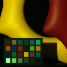
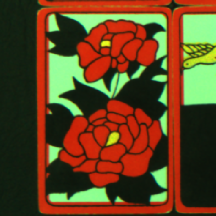
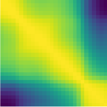
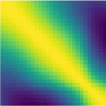
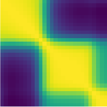
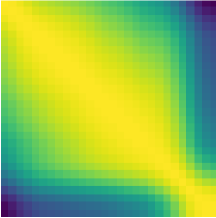
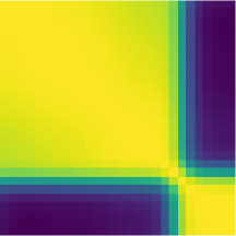
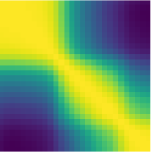
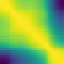
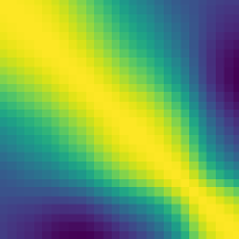
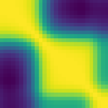
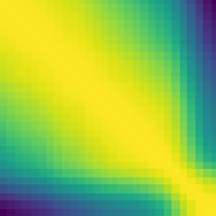
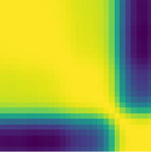
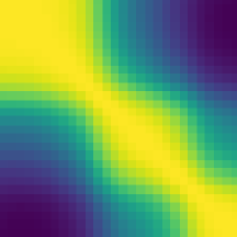
Figure 11: Visualization of the spectral correlation. Top: RGB contents of the benchmark testing data. Middle: spectral correlation coefficient matrices of the ground truth ($28$$\times$$28$). Bottom: Corresponding matrices by the proposed method.

$S^{2}$-attn Discussion. We firstly investigate the differences among proposed $S^{2}$-attn blocks by comparing the reconstruction performances. Notably, we enhance the Spa and Spe blocks for a comparable computational cost, as shown by the dash boxes in Fig. 4. In Table V, we report the model size (#params), computational complexity by floating point operations (FLOPs), and the reconstruction performances comprehensively. For the metric comparison, the Parall-SS block yields the best result, i.e., 36.31dB/0.9569 in terms of the PSNR/SSIM, while the SpeSpe block shows more limitations toward a high-fidelity reconstruction among all architecture designs. By comparison, the Parall-SS block empowers 1.13dB/0.0033 boost. For the computational burden, the SpaSpa block requires the most computational overhead, while the SpeSpe block takes the minimum computation. Note that both spatial-spectral attention structures achieve superior performances than the solely spatial/spectral mechanisms, indicating a better data clue exploitation of joint modeling. Specifically, the Parall-SS outperforms the Sequn-SS under the same computational burden, which makes sense considering the two-fold data characteristics. (1) The spatial attention modeling infers the visually grounded semantics, which is determined by the physical object of capturing by the hardware. The spectral attention describes the embedding channel interplay, which heavily relies on the pre-determined wavelengths. Thereby, paralleled structure attains the most modeling independences, respectively. (2) The learnable feature fusion in Parall-SS enables embedding interaction in each block, bringing more flexibility than the Sequn-SS.

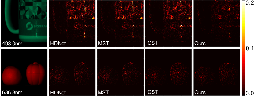
Figure 12: Reconstruction difficulty maps ($|\widehat{\mathbf{F}}$$-$$\mathbf{F}|_{\texttt{chl}}$) in masked areas. Lower intensity indicates a better retrieval capacity.

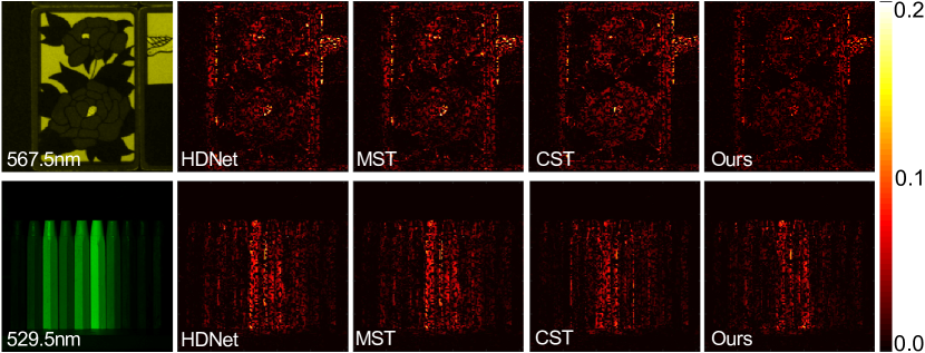
Figure 13: Reconstruction difficulty maps ($|\widehat{\mathbf{F}}$$-$$\mathbf{F}|_{\texttt{chl}}$) in masked areas. Lower intensity indicates a better retrieval capacity.

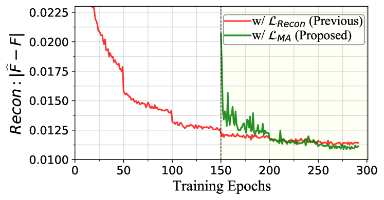
Figure 14: Convergence analysis of the reconstruction. Previous strategy employs the Recon term, i.e., $\mathcal{L}_{\texttt{Recon}}$$=$$|\widehat{\mathbf{F}}-\mathbf{F}|$. With the mask-aware learning, the reconstruction converges toward a lower scale. The $\mathcal{L}_{\texttt{MA}}$ follows 150-epoch pre-training.

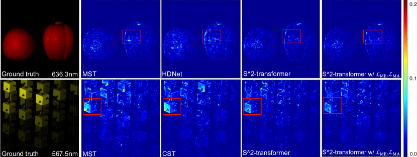
Figure 15: Reconstruction difficulty maps ($|\widehat{\mathbf{F}}-\mathbf{F}|_{\texttt{chl}}$) on simulation data. Lower intensity indicates a better retrieval.

Parallel Spatial-Spectral Attention Analysis. Following the above observations, we put emphasize on the Parall-SS block. First of all, we visualize the fused feature embedding within the attention blocks at different depth. There are total 24 blocks given $K$$=$$4$ and $L$$=$$6$. In Fig. 10, we visualize the feature maps of the embedding with random channel indices and depths. By observation, the representations in deeper blocks are closer to the visual semantics, with the deep blocks actually presents a similar abstracting ability (e.g., blk 22 and blk 24 of Scene 10 in Fig. 10). Based on this observation, we exploit the inherent interpretability from the top of the network (i.e., 22$\sim$24 blocks). In Fig. 9, we present the feature embedding right after the $f_{\texttt{Spa-MSA}}(\cdot)$ and $f_{\texttt{Spe-MSA}}(\cdot)$, respectively. The evidences across different data indicate that one functionality of the $f_{\texttt{Spe-MSA}}(\cdot)$ is in a way of edge detector. The $f_{\texttt{Spa-MSA}}(\cdot)$ conversely collects the fine-grained visual details. This observation coincides with our motivations. (1) Spatial attention allows a fine-grained visual detail modeling by attending the total number of $H$$\times$$W$ tokens. (2) The $f_{\texttt{Spe-MSA}}(\cdot)$ describes the 2D token relations by a scalar attention value regardless of the token spatial size, which indicates a heterogeneous spatial expressiveness across the 2D token plane, considering the finite modeling capacity. In our case, it ultimately depends on the most discriminative regions, i.e., edges, for the feature channel differentiating. Since the inconsistent representation space between the embedding ($C$$=$60) and the hyperspectral signal ($N{{}_{\lambda}}$$=$$28$), we directly observe the spectral distribution of the predictions upon Parall-SS. As shown in Fig. 11, each image possesses a unique distribution. The proposed network retrieves the spectrum patterns properly. Due to the better performance and interpretability of the Parall-SS, we finalize the network structure and conduct the experiments in the following by this block.

4.4 Mask-aware Learning

TABLE VI: Ablation study on mask-aware learning. Note that $\mathcal{L}_{\texttt{ME}}$ is employed in pre-training for the proposed method.

Loss types	Recon	ME	MA	pre-train	PSNR(dB)	SSIM
Previous	✓	✗	✗	✗	36.31	0.9569
$\mathcal{L}_{\texttt{ME}}$	✓	✓	✗	✗	36.32	0.9569
$\mathcal{L}_{\texttt{MA}}$	✓	✓	✓	✗	34.88	0.9496
$\mathcal{L}_{\texttt{ME}}$ , $\mathcal{L}_{\texttt{MA}}$	✓	✓	✓	✓	36.48	0.9584

Convergence Analysis. We firstly conduct an ablation study for the proposed mask-aware learning in Table VI. We choose the $|\widehat{\mathbf{F}}-\mathbf{F}|$ as the Previous setting and all experiments follow the same optimization configurations (refer to Section 4.1 for more details). By comparison, a complete mask-aware learning treatment enables 0.17dB/0.0015 improvement over the baseline. Besides, solely employing either $\mathcal{L}_{\texttt{ME}}$ or $\mathcal{L}_{\texttt{MA}}$ hardly benefits the reconstruction. (1) The mask-encoding (ME) term introduced in $\mathcal{L}_{\texttt{ME}}$ penalizes the shallow parts of the network. Its effect weakens as the network deepens. (2) The mask-aware (MA) term infers the masked regions upon the well-approximated $\widehat{\mathbf{F}}$, which is unattainable in early training steps. We further analyze the convergence of the reconstruction by directly observing the Recon term. As shown in Fig. 14, the absolute error between the $\widehat{\mathbf{F}}$ and $\mathbf{F}$ is further minimized when applying MA. Since the $\mathcal{L}_{\texttt{MA}}$ prioritizes the masked region with higher penalty. A more precised reconstruction accordingly contributes to a globally-averaged fidelity. We perceptually show this point below.

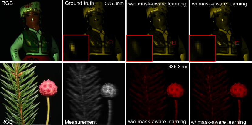
Figure 16: Visual comparison of the proposed mask-aware learning. Top: simulation data. Bottom: real data. Note that the ground truth is unattainable in practice. Mask-aware learning enables more texture retrieval by comparison.

Data Uncertainty. We firstly compare the empirical difficulties among different methods. Spectral channels are selected at random and the masked regions are emphasized, i.e., $|\widehat{\mathbf{F}}-\mathbf{F}|$$\odot$$(\mathbf{1}-\mathbf{M})$, where $\odot$ denotes a pixel-wise multiplication. As shown by the Fig. 12$\sim$13, the proposed method yields better retrieval. Identifying the masked areas is non-trivial, since the commonly used L1 or L2 norms hardly distinguish aleatoric uncertainty caused by the internal high-frequency textures and the external hardware encoding (i.e., masking). This leads to a common modeling behaviour. In Fig. 15, we further visualize the reconstruction difficulties among compared methods and our ablated models. In line with the convergence curve in Fig. 14, the $\mathcal{L}_{MA}$ enhances the reconstruction globally. Better approximation of the masked areas potentially benefits the neighbored pixel estimation owning to the spatial locality property of the model. We finally visualize both simulation and real predictions of the ablated model in Fig. 16. By the zoom-in windows, mask-aware learning contributes to a high-fidelity reconstruction.

5 Conclusion

In this work, we revealed two-fold data loss that impede a high-fidelity reconstruction of hyperspectral images by observing the physical encoding procedure of CASSI. For the entangled data loss, we resorted to exploit the hyperspectral image characteristics for a better information compensation upon the 2D measurement. We introduced the $S^{2}$-Transformer by systematically discussing different self-attention mechanisms. The empirical evidence demonstrated the different functionalities of both spatial and spectral attention under a paralleled arrangement. For the masked data loss, we identify and take advantage of the optical-induced data uncertainty in a pixel-wise manner by prioritizing the masked pixels adaptively throughout the training. We theoretically and empirically presented the convergence tendencies of the proposed learning strategy upon both mask and unmasked regions. Our proposed method achieves superior performance compared with existing state-of-the-arts quantitatively and perceptually. Besides, this work serves as the first attempt to expedite the interpretability of designing deep reconstruction networks for HSI from the physical scope. We hope our discussions shed light on the future Transformer design for the HSI community.

Jiamian Wang received B.Eng. degree from electronic information engineering from Tianjin University, Tianjin, China, in 2018 and M.S. degree from University of Southern California, USA, in 2020. He is currently pursuing the Ph.D. degree with the Department of Computing and Information Sciences, Rochester Institute of Technology, USA. His research interests include hyperspectral imaging and uncertianty estimation.

Kunpeng Li (S’18-M’21) received the B.Eng. degree in Information Engineering from South China University of Technology, China and Ph.D. degree in Computer Engineering, Northeastern University, Boston, MA. He is a Research Scientist at Meta Reality Labs, CA. He has also spent time at Google Research, Adobe Research etc. as a research intern. His research interests include learning with limited supervision, scene understanding, vision & language, and video understanding.

Yulun Zhang is a postdoctoral researcher at Computer Vision Lab, ETH Zürich, Switzerland. He obtained the Ph.D. degree from the Department of ECE, Northeastern University, USA, in 2021. He also worked as a research fellow in Harvard University. Before that, he received the B.E. degree from the School of Electronic Engineering, Xidian University, China, in 2013 and the M.E. degree from the Department of Automation, Tsinghua University, China, in 2017. His research interests include image/video restoration and synthesis, biomedical image analysis, model compression, and computational imaging.

Xin Yuan (SM’16) received the BEng and MEng degrees from Xidian University, in 2007 and 2009, respectively, and the PhD from the Hong Kong Polytechnic University, in 2012. He is currently an Associate Professor at Westlake University. He was a video analysis and coding lead researcher at Bell Labs, Murray Hill, NJ, USA from 2015 to 2021. Prior to this, he was a Post-Doctoral Associate in the Department of Electrical and Computer Engineering, Duke University from 2012 to 2015. His research interests are computational imaging and machine learning. He has been the Associate Editor of Pattern Recognition (2019-), International Journal of Pattern Recognition and Artificial Intelligence (2020-) and Chinese Optics Letters (2021-). He led the special issue of "Deep Learning for High Dimensional Sensing" in the IEEE Journal of Selected Topics in Signal Processing in 2022.

Zhiqiang Tao received the B.Eng. degree in software engineering from the School of Computer Software, and the M.Eng. degree in computer science from the School of Computer Science and Technology, Tianjin University, Tianjin, China, in 2012 and 2015, respectively. He received the Ph.D. degree from the Department of Electrical and Computer Engineering, Northeastern University, Boston MA, 2020. He has been a Tenure-Track Assistant Professor at the School of Information, Rochester Institute of Technology, since 2022. Before that, he was an Assistant Professor at the Department of Computer Science and Engineering, Santa Clara University, from 2020 to 2022. He has served as the Associate Editor of Neurocomputing (2022-), a reviewer for several IEEE Transactions, including TPAMI, TKDE, TNNLS, TIP, TCYB, TCSVT, TMM, and a program committee member for conferences NeurIPS, ICML, KDD, ICLR, AAAI, IJCAI, CVPR, ICCV, ECCV, CIKM, and WSDM. His research interests include representation learning, sequence mining, AutoML, and interpretability.

References

- [1] Y. Fu, Y. Zheng, H. Huang, I. Sato, and Y. Sato, “Hyperspectral image super-resolution with a mosaic rgb image,” IEEE Transactions on Image Processing, vol. 27, no. 11, pp. 5539–5552, 2018.
- [2] Y. Fu, T. Zhang, Y. Zheng, D. Zhang, and H. Huang, “Hyperspectral image super-resolution with optimized rgb guidance,” in Proceedings of the IEEE/CVF Conference on Computer Vision and Pattern Recognition (CVPR), 2019, pp. 11 661–11 670.
- [3] G. Lu and B. Fei, “Medical hyperspectral imaging: a review,” Journal of biomedical optics, vol. 19, no. 1, p. 010901, 2014.
- [4] J. Suo, W. Zhang, J. Gong, X. Yuan, D. J. Brady, and Q. Dai, “Computational imaging and artificial intelligence: The next revolution of mobile vision,” arXiv preprint arXiv:2109.08880, 2021.
- [5] M. E. Gehm, R. John, D. J. Brady, R. M. Willett, and T. J. Schulz, “Single-shot compressive spectral imaging with a dual-disperser architecture,” Optics express, vol. 15, no. 21, pp. 14 013–14 027, 2007.
- [6] A. Wagadarikar, R. John, R. Willett, and D. Brady, “Single disperser design for coded aperture snapshot spectral imaging,” Applied optics, vol. 47, no. 10, pp. B44–B51, 2008.
- [7] X. Yuan, D. J. Brady, and A. K. Katsaggelos, “Snapshot compressive imaging: Theory, algorithms, and applications,” IEEE Signal Processing Magazine, vol. 38, no. 2, pp. 65–88, 2021.
- [8] J. M. Bioucas-Dias and M. A. Figueiredo, “A new twist: Two-step iterative shrinkage/thresholding algorithms for image restoration,” IEEE Transactions on Image processing, vol. 16, no. 12, pp. 2992–3004, 2007.
- [9] Y. Liu, X. Yuan, J. Suo, D. J. Brady, and Q. Dai, “Rank minimization for snapshot compressive imaging,” IEEE transactions on pattern analysis and machine intelligence, vol. 41, no. 12, pp. 2990–3006, 2018.
- [10] J. Ma, X.-Y. Liu, Z. Shou, and X. Yuan, “Deep tensor admm-net for snapshot compressive imaging,” in Proceedings of the IEEE/CVF International Conference on Computer Vision (ICCV), 2019, pp. 10 223–10 232.
- [11] J. Bioucas-Dias and M. Figueiredo, “A new TwIST: Two-step iterative shrinkage/thresholding algorithms for image restoration,” IEEE Transactions on Image Processing, vol. 16, no. 12, pp. 2992–3004, December 2007.
- [12] M. A. Figueiredo, R. D. Nowak, and S. J. Wright, “Gradient projection for sparse reconstruction: Application to compressed sensing and other inverse problems,” IEEE Journal of selected topics in signal processing, vol. 1, no. 4, pp. 586–597, 2007.
- [13] L. Wang, Z. Xiong, G. Shi, F. Wu, and W. Zeng, “Adaptive nonlocal sparse representation for dual-camera compressive hyperspectral imaging,” IEEE transactions on pattern analysis and machine intelligence, vol. 39, no. 10, pp. 2104–2111, 2016.
- [14] Y. Cai, J. Lin, X. Hu, H. Wang, X. Yuan, Y. Zhang, R. Timofte, and L. Van Gool, “Mask-guided spectral-wise transformer for efficient hyperspectral image reconstruction,” in Proceedings of the IEEE/CVF Conference on Computer Vision and Pattern Recognition (CVPR), 2022, pp. 17 502–17 511.
- [15] Z. Meng, J. Ma, and X. Yuan, “End-to-end low cost compressive spectral imaging with spatial-spectral self-attention,” in European Conference on Computer Vision (ECCV), August 2020.
- [16] Y. Cai, J. Lin, X. Hu, H. Wang, X. Yuan, Y. Zhang, R. Timofte, and L. Van Gool, “Coarse-to-fine sparse transformer for hyperspectral image reconstruction,” in European Conference on Computer Vision (ECCV). Springer, 2022, pp. 686–704.
- [17] L. Wang, C. Sun, M. Zhang, Y. Fu, and H. Huang, “Dnu: Deep non-local unrolling for computational spectral imaging,” in Proceedings of the IEEE/CVF Conference on Computer Vision and Pattern Recognition (CVPR), June 2020.
- [18] S. Zheng, Y. Liu, Z. Meng, M. Qiao, Z. Tong, X. Yang, S. Han, and X. Yuan, “Deep plug-and-play priors for spectral snapshot compressive imaging,” Photonics Research, vol. 9, no. 2, pp. B18–B29, 2021.
- [19] S. Jalali and X. Yuan, “Snapshot compressed sensing: Performance bounds and algorithms,” IEEE Transactions on Information Theory, vol. 65, no. 12, pp. 8005–8024, 2019.
- [20] A. Dosovitskiy, L. Beyer, A. Kolesnikov, D. Weissenborn, X. Zhai, T. Unterthiner, M. Dehghani, M. Minderer, G. Heigold, S. Gelly, J. Uszkoreit, and N. Houlsby, “An image is worth 16x16 words: Transformers for image recognition at scale,” in International Conference on Learning Representations (ICLR), 2021.
- [21] A. Kendall and Y. Gal, “What uncertainties do we need in bayesian deep learning for computer vision?” Advances in neural information processing systems (NeurIPS), vol. 30, 2017.
- [22] Q. Ning, W. Dong, X. Li, J. Wu, and G. Shi, “Uncertainty-driven loss for single image super-resolution,” Advances in Neural Information Processing Systems (NeurIPS), vol. 34, 2021.
- [23] E. J. Candès, J. Romberg, and T. Tao, “Robust uncertainty principles: Exact signal reconstruction from highly incomplete frequency information,” IEEE Transactions on information theory, vol. 52, no. 2, pp. 489–509, 2006.
- [24] D. L. Donoho, “Compressed sensing,” IEEE Transactions on information theory, vol. 52, no. 4, pp. 1289–1306, 2006.
- [25] X. Cao, H. Du, X. Tong, Q. Dai, and S. Lin, “A prism-mask system for multispectral video acquisition,” IEEE transactions on pattern analysis and machine intelligence, vol. 33, no. 12, pp. 2423–2435, 2011.
- [26] X. Yuan, T.-H. Tsai, R. Zhu, P. Llull, D. Brady, and L. Carin, “Compressive hyperspectral imaging with side information,” IEEE Journal of Selected Topics in Signal Processing, vol. 9, no. 6, pp. 964–976, September 2015.
- [27] Y. Wu, I. O. Mirza, G. R. Arce, and D. W. Prather, “Development of a digital-micromirror-device-based multishot snapshot spectral imaging system,” Opt. Lett., vol. 36, no. 14, pp. 2692–2694, Jul 2011.
- [28] D. Kittle, K. Choi, A. Wagadarikar, and D. J. Brady, “Multiframe image estimation for coded aperture snapshot spectral imagers,” Applied optics, vol. 49, no. 36, pp. 6824–6833, 2010.
- [29] T. Huang, W. Dong, X. Yuan, J. Wu, and G. Shi, “Deep gaussian scale mixture prior for spectral compressive imaging,” in Proceedings of the IEEE/CVF Conference on Computer Vision and Pattern Recognition (CVPR), 2021, pp. 16 216–16 225.
- [30] L. Wang, Z. Xiong, D. Gao, G. Shi, and F. Wu, “Dual-camera design for coded aperture snapshot spectral imaging,” Applied optics, vol. 54, no. 4, pp. 848–858, 2015.
- [31] L. Wang, Z. Xiong, D. Gao, G. Shi, W. Zeng, and F. Wu, “High-speed hyperspectral video acquisition with a dual-camera architecture,” in 2015 IEEE Conference on Computer Vision and Pattern Recognition (CVPR), June 2015, pp. 4942–4950.
- [32] L. Wang, Z. Xiong, H. Huang, G. Shi, F. Wu, and W. Zeng, “High-speed hyperspectral video acquisition by combining nyquist and compressive sampling,” IEEE Transactions on Pattern Analysis and Machine Intelligence, 2018.
- [33] H. Arguello, H. Rueda, Y. Wu, D. W. Prather, and G. R. Arce, “Higher-order computational model for coded aperture spectral imaging,” Applied optics, vol. 52, no. 10, pp. D12–D21, 2013.
- [34] X. Yuan, “Generalized alternating projection based total variation minimization for compressive sensing,” in 2016 IEEE International Conference on Image Processing (ICIP). IEEE, 2016, pp. 2539–2543.
- [35] L. Wang, C. Sun, Y. Fu, M. H. Kim, and H. Huang, “Hyperspectral image reconstruction using a deep spatial-spectral prior,” in Proceedings of the IEEE/CVF Conference on Computer Vision and Pattern Recognition (CVPR), 2019.
- [36] J. Ma, X. Liu, Z. Shou, and X. Yuan, “Deep tensor admm-net for snapshot compressive imaging,” in IEEE/CVF Conference on Computer Vision (ICCV), 2019.
- [37] Y. Fu, Z. Liang, and S. You, “Bidirectional 3d quasi-recurrent neural network for hyperspectral image super-resolution,” IEEE Journal of Selected Topics in Applied Earth Observations and Remote Sensing, vol. 14, pp. 2674–2688, 2021.
- [38] X. Zhang, Y. Zhang, R. Xiong, Q. Sun, and J. Zhang, “Herosnet: Hyperspectral explicable reconstruction and optimal sampling deep network for snapshot compressive imaging,” in Proceedings of the IEEE/CVF Conference on Computer Vision and Pattern Recognition (CVPR), 2022, pp. 17 532–17 541.
- [39] S. Boyd, N. Parikh, E. Chu, B. Peleato, J. Eckstein et al., “Distributed optimization and statistical learning via the alternating direction method of multipliers,” Foundations and Trends® in Machine learning, vol. 3, no. 1, pp. 1–122, 2011.
- [40] L. Wang, C. Sun, M. Zhang, Y. Fu, and H. Huang, “Dnu: Deep non-local unrolling for computational spectral imaging,” in Proceedings of the IEEE/CVF Conference on Computer Vision and Pattern Recognition (CVPR), 2020, pp. 1661–1671.
- [41] S. H. Chan, X. Wang, and O. A. Elgendy, “Plug-and-play admm for image restoration: Fixed-point convergence and applications,” IEEE Transactions on Computational Imaging, vol. 3, no. 1, pp. 84–98, 2016.
- [42] M. Qiao, X. Liu, and X. Yuan, “Snapshot spatial–temporal compressive imaging,” Optics letters, vol. 45, no. 7, pp. 1659–1662, 2020.
- [43] Z. Meng, M. Qiao, J. Ma, Z. Yu, K. Xu, and X. Yuan, “Snapshot multispectral endomicroscopy,” Optics Letters, vol. 45, no. 14, pp. 3897–3900, 2020.
- [44] X. Miao, X. Yuan, Y. Pu, and V. Athitsos, “-net: Reconstruct hyperspectral images from a snapshot measurement,” in IEEE/CVF Conference on Computer Vision (ICCV), 2019.
- [45] L. Wang, T. Zhang, Y. Fu, and H. Huang, “Hyperreconnet: Joint coded aperture optimization and image reconstruction for compressive hyperspectral imaging,” IEEE Transactions on Image Processing, vol. 28, no. 5, pp. 2257–2270, May 2019.
- [46] Z. Cheng, B. Chen, R. Lu, Z. Wang, H. Zhang, Z. Meng, and X. Yuan, “Recurrent neural networks for snapshot compressive imaging,” IEEE Transactions on Pattern Analysis and Machine Intelligence, 2022.
- [47] X. Hu, Y. Cai, J. Lin, H. Wang, X. Yuan, Y. Zhang, R. Timofte, and L. Van Gool, “Hdnet: High-resolution dual-domain learning for spectral compressive imaging,” in Proceedings of the IEEE/CVF Conference on Computer Vision and Pattern Recognition (CVPR), 2022, pp. 17 542–17 551.
- [48] A. Vaswani, N. Shazeer, N. Parmar, J. Uszkoreit, L. Jones, A. N. Gomez, Ł. Kaiser, and I. Polosukhin, “Attention is all you need,” Advances in neural information processing systems (NeurIPS), vol. 30, 2017.
- [49] Y. Bengio, J. Louradour, R. Collobert, and J. Weston, “Curriculum learning,” in Proceedings of the 26th Annual International Conference on Machine Learning (ICML), 2009, p. 41–48.
- [50] X. Wang, Y. Chen, and W. Zhu, “A survey on curriculum learning,” IEEE Transactions on Pattern Analysis and Machine Intelligence, 2021.
- [51] Z. Meng, S. Jalali, and X. Yuan, “Gap-net for snapshot compressive imaging,” arXiv preprint arXiv:2012.08364, 2020.
- [52] J. Wang, Y. Zhang, X. Yuan, Y. Fu, and Z. Tao, “A new backbone for hyperspectral image reconstruction,” arXiv preprint arXiv:2108.07739, 2021.
- [53] J. Liang, J. Cao, G. Sun, K. Zhang, L. Van Gool, and R. Timofte, “Swinir: Image restoration using swin transformer,” in Proceedings of the IEEE/CVF International Conference on Computer Vision (ICCV), 2021, pp. 1833–1844.
- [54] Z. Liu, Y. Lin, Y. Cao, H. Hu, Y. Wei, Z. Zhang, S. Lin, and B. Guo, “Swin transformer: Hierarchical vision transformer using shifted windows,” in Proceedings of the IEEE/CVF International Conference on Computer Vision (CVPR), 2021, pp. 10 012–10 022.
- [55] J. L. Ba, J. R. Kiros, and G. E. Hinton, “Layer normalization,” arXiv preprint arXiv:1607.06450, 2016.
- [56] H. Bao, L. Dong, F. Wei, W. Wang, N. Yang, X. Liu, Y. Wang, J. Gao, S. Piao, M. Zhou et al., “Unilmv2: Pseudo-masked language models for unified language model pre-training,” in International Conference on Machine Learning (ICML). PMLR, 2020, pp. 642–652.
- [57] H. Hu, J. Gu, Z. Zhang, J. Dai, and Y. Wei, “Relation networks for object detection,” in Proceedings of the IEEE conference on computer vision and pattern recognition (CVPR), 2018, pp. 3588–3597.
- [58] P. Shaw, J. Uszkoreit, and A. Vaswani, “Self-attention with relative position representations,” arXiv preprint arXiv:1803.02155, 2018.
- [59] Z. Meng and X. Yuan, “Perception inspired deep neural networks for spectral snapshot compressive imaging,” in 2021 IEEE International Conference on Image Processing (ICIP). IEEE, 2021, pp. 2813–2817.
- [60] F. Yasuma, T. Mitsunaga, D. Iso, and S. K. Nayar, “Generalized assorted pixel camera: postcapture control of resolution, dynamic range, and spectrum,” IEEE transactions on image processing, vol. 19, no. 9, pp. 2241–2253, 2010.
- [61] I. Choi, D. S. Jeon, G. Nam, D. Gutierrez, and M. H. Kim, “High-quality hyperspectral reconstruction using a spectral prior,” ACM Trans. Graph., vol. 36, no. 6, nov 2017.
- [62] D. P. Kingma and J. Ba, “Adam: A method for stochastic optimization,” arXiv preprint arXiv:1412.6980, 2014.
- [63] Z. Wang, A. C. Bovik, H. R. Sheikh, and E. P. Simoncelli, “Image quality assessment: from error visibility to structural similarity,” IEEE transactions on image processing, vol. 13, no. 4, pp. 600–612, 2004.
- [64] A. Mittal, R. Soundararajan, and A. C. Bovik, “Making a “completely blind” image quality analyzer,” IEEE Signal processing letters, vol. 20, no. 3, pp. 209–212, 2012.