Face Super-Resolution Using Stochastic Differential Equations

Abstract

Diffusion models have proven effective for various applications such as images, audio and graph generation. Other important applications are image super-resolution and the solution of inverse problems. More recently, some works have used stochastic differential equations (SDEs) to generalize diffusion models to continuous time. In this work, we introduce SDEs to generate super-resolution face images. To the best of our knowledge, this is the first time SDEs have been used for such an application. The proposed method provides an improved peak signal-to-noise ratio (PSNR), structural similarity index measure (SSIM), and consistency than the existing super-resolution methods based on diffusion models. In particular, we also assess the potential application of this method for the face recognition task. A generic facial feature extractor is used to compare the super-resolution images with the ground truth, and superior results were obtained compared with other methods. Our code is publicly available at https://github.com/marcelowds/sr-sde.

I Introduction

Probabilistic approaches have been successfully applied to data generation. Two main discrete models are known as Denoising Diffusion Probabilistic Models (DDPM) [1, 2] and Score matching with Langevin dynamics (SMLD) [3].

Inspired by considerations from non-equilibrium thermodynamics, in the DDPM, a Markov chain is used to model the forward and reverse processes of a diffusion model. In the forward process, random Gaussian noise is added to the clean image until a pure noisy image is obtained. A network is trained to predict the noise level of the image at each step. To generate an image in the reverse process, a pure Gaussian noise is considered as the initial state of a Markov chain. The network is used to iteratively denoise the image until a clean image is obtained.

Similar to DDPM, the SMLD model consists of perturbing the data with different scales of random Gaussian noise. A network conditioned at the noise level is trained to learn the gradient of the log probability density with respect to data. The Langevin dynamics [4] is used for the data generation process to remove the noise from the data iteratively. Starting from high noise levels, the process runs until low noise levels are reached and the generated images have distributions indistinguishable from the original data distribution. These two classes of models are part of score-based generative models.

Score-based generative models have been successfully applied to a wide range of different data, such as the generation of audio [5], graphs [6] and shapes [7] as well as for image synthesis, achieving results even better than Generative Adversarial Networks (GANs) [8], image edition [9], text-to-image translation [10], general inverse problems [11, 12], super-resolution [13, 14], among others. For the super-resolution task, Saharia et al. [13] and Li et al. [14] adapted the DDPM models to generate super-resolution images using low-resolution images as a guide to a Markov chain. In [12], super-resolution was treated as a special case of an inverse problem.

In [15], the authors presented a generalization of score-based models to continuous time using a stochastic differential equation (SDE). The DDPM and SMLD models are considered particular cases of a general SDE. The generalization of the DDPM and SMLD models are called variation preserving (VP) and variation exploding (VE), respectively. In [15], it is also presented a third model named subVP, which has the variance preserved during the diffusion process but is limited by the variance of the VP process. The developed methods reached record-breaking results for unconditional image generation, which is performed by solving a reverse SDE. More recently, in [16, 17, 18], the SDE score-based models are further developed, focusing on decreasing the execution time, optimizing the image generation process, and improving high-resolution image synthesis.

In this work, the continuous version of diffusion models described through an SDE in [15] is adapted to deal with the face super-resolution problem. As far as we know, this is the first time that SDEs are used to face super-resolution images. We evaluate four different algorithms: SDE-VP, SDE-subVP, SDE-VE and SDE-VE cs. The robustness of the obtained models is demonstrated by the generation of detailed and high-quality super-resolution images.

The peak signal-to-noise ratio (PSNR) and structural similarity index measure (SSIM) values achieved are similar to those obtained by other super-resolution methods based on diffusion models. However, considering that these metrics are not strongly correlated with how humans perceive image quality [19, 13], we conducted an additional experiment to demonstrate the superiority of the proposed method. The high-resolution (HR) and super-resolution (SR) images are provided to a VGG-Face network [20] for obtaining a compact feature descriptor and measuring the average cosine similarity between the corresponding HR and SR images. The obtained results are more promising than existing methods. We also show that if we only rely on the PSNR metric, this does not always provide the best images for face recognition. Moreover, our super-resolution method is based on denoising, so our method is particularly suitable for surveillance scenarios where the image quality is low and noisy.

The remaining of this paper is organized as follows: Section II contains the theoretical background behind the proposed method, while Section III describes our experiments and results. Finally, section IV concludes the paper.

II Theoretical background

II-A Stochastic differential equations and super-resolution

A continuous diffusion process $\{x(t)\}_{t=0}^{T}$ can be modeled by the Itô SDE

$$\mathrm{d}\mathbf{x}=\mathbf{f}(\mathbf{x},t)\mathrm{d}t+g(t)\mathrm{d}\mathbf{w},$$ (1)

where $\mathbf{f}(\mathbf{x},t)$ is the drift coefficient, $g(t)$ is a diffusion coefficient, and $\mathbf{w}$ is a Wiener process. For more details about Itô SDE and Wiener process, see [21, 4]. In [22], it was shown that it is possible to reverse the diffusion process (Eq. 1) using another diffusion process given by

$$\mathrm{d}\mathbf{x}=[\mathbf{f}(\mathbf{x},t)-g(t)^{2}\nabla_{\mathbf{x}}\log p_{t}(\mathbf{x})]\mathrm{d}t+g(t)\mathrm{d}\bar{\mathbf{w}},$$ (2)

where $\mathrm{d}\bar{\mathbf{w}}$ is a Wiener process running backwards in time.

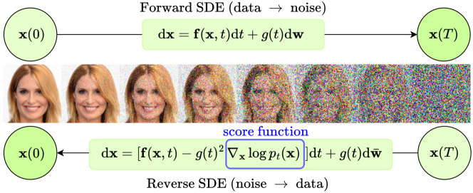
Figure 1: Forward and reverse processes. Adapted from [15].

In [15], the authors used a deep neural network $s_{\theta}(\mathbf{x}(t),t)$ to learn $\nabla_{\mathbf{x}}\log p_{t}(\mathbf{x})$ during the forward process. Once this gradient is learned, the reverse process (Eq. 2) is run, changing $\nabla_{\mathbf{x}}\log p_{t}(\mathbf{x})$ by $s_{\theta}(\mathbf{x}(t),t)$ to generate a sample $\mathbf{x}(0)\sim p_{0}$ (see Fig. 1). As we are dealing with the super-resolution problem, in this work, we also use a down-sampled version $\mathbf{y}$ of the image $\mathbf{x}$ as input to the network, denoted by $s_{\theta}(\mathbf{x}(t),\mathbf{y},t)$. To generate a super-resolution image, during the reverse process we initially use a noisy image $\mathbf{x}(T)$ to iteratively transform it on $\mathbf{x}(0)$, using $\mathbf{y}$ as a guide to the stochastic process.

To train the network, we must find the parameters $\theta$ of $s_{\theta}(\mathbf{x}(t),\mathbf{y},t)$ such that $\nabla_{\mathbf{x}}\log p_{t}(\mathbf{x})$ can be well approximated by the network. For this purpose, we must optimize the following function [23]

$$\min_{\theta}\mathbb{E}_{t\sim\mathcal{U}[0,T]}\mathbb{E}_{\mathbf{x}_{0}\sim p(\mathbf{x}_{0})}\mathbb{E}_{\mathbf{x}(t)\sim p_{t}(\mathbf{x}(t)|\mathbf{x}(0)}\big{[}\lambda(t)$$

$$\times\,\|s_{\theta}(\mathbf{x}(t),\mathbf{y},t)-\nabla_{\mathbf{x}(t)}\log p(\mathbf{x}(t)|\mathbf{x}(0))\|_{2}^{2}\big{]},$$ (3)

where $\lambda(t)$ is a positive weighting function. In Eq. 3, we need to compute $p(\mathbf{x}(t)|\mathbf{x}(0))$, but if $\mathbf{f}(\mathbf{x},t)$ from Eq. 1 is an affine function, the distribution $p(\mathbf{x}_{t}|\mathbf{x}_{0})$ is a normal distribution where the mean $\boldsymbol{\mu}(t)$ and variance $\boldsymbol{\Sigma}(t)$ evolve according to the following differential equations [4]

$$\frac{\mathrm{d}\boldsymbol{\mu}(t)}{\mathrm{d}t}=\mathbb{E}[\mathbf{f}(\mathbf{x},t)]$$ (4)

and

$$\frac{\mathrm{d}\boldsymbol{\Sigma}(t)}{\mathrm{d}t}=\mathbb{E}[\mathbf{f}(\mathbf{x},t)(\mathbf{x}-\boldsymbol{\mu}(t))^{\top}+(\mathbf{x}-\boldsymbol{\mu}(t))\mathbf{f}^{\top}(\mathbf{x},t)]$$

$$+g^{2}(t)\mathbf{I}.$$ (5)

In the VE, VP and subVP cases described in [15] we have $\mathbf{f}(\mathbf{x},t)$ and $g(t)$ given respectively by

$$\mathbf{f}(\mathbf{x},t)=\mathbf{0},\quad g(t)=\sqrt{\frac{\mathrm{d}\sigma^{2}(t)}{\mathrm{d}t}},$$ (6)

$$\mathbf{f}(\mathbf{x},t)=-\frac{1}{2}\beta(t)\mathbf{x},\quad g(t)=\sqrt{\beta(t)}$$ (7)

and

$$\mathbf{f}(\mathbf{x},t)=-\frac{1}{2}\beta(t)\mathbf{x},\,g(t)=\sqrt{\beta(t)\left(1-e^{-2\int_{0}^{t}\beta(s)\mathrm{d}s}\right)},$$ (8)

where $\sigma(t)$ and $\beta(t)$ are functions which describe the level of noise added to the data at each time.

For all the three models, the drift coefficients are affine functions and the mean and variance are computed analytically using Eq. 4 and Eq. 5. The results for the mean and variance of the VE, VP and subVP models are obtained in [15] and are given respectively by

$$\boldsymbol{\mu}(t)=\mathbf{x}(0),\,\,\boldsymbol{\Sigma}(t)=[\sigma^{2}(t)-\sigma^{2}(0)]\mathbf{I},$$ (9)

$$\boldsymbol{\mu}(t)=\mathbf{x}(0)e^{-\frac{1}{2}\int_{0}^{t}\beta(s)\mathrm{d}s},\,\,\boldsymbol{\Sigma}(t)=[1-e^{-\frac{1}{2}\int_{0}^{t}\beta(s)\mathrm{d}s}]\mathbf{I},$$ (10)

and

$$\boldsymbol{\mu}(t)=\mathbf{x}(0)e^{-\frac{1}{2}\int_{0}^{t}\beta(s)\mathrm{d}s},\,\,\boldsymbol{\Sigma}(t)=[1-e^{-\frac{1}{2}\int_{0}^{t}\beta(s)\mathrm{d}s}]^{2}\mathbf{I}.$$ (11)

With these three equations, it is possible to compute $p(\mathbf{x}_{t}|\mathbf{x}_{0})$ and calculate the loss function (Eq. 3) during the training process.

Following [15], we choose $\sigma(t)=\sigma_{min}\left(\sigma_{max}/\sigma_{min}\right)^{t}$ and $\beta(t)=\bar{\beta}_{min}+(\bar{\beta}_{max}-\bar{\beta}_{min})t$ to describe the noise level.

II-B Solving the SDE

After the training is performed and the function $s_{\theta}$ is obtained, we need to solve the reverse diffusion (Eq. 2) from $t=T$ to $t=0$ in order to obtain the super-resolution images. For this purpose, we use the Algorithm (1), which is composed of two main functions, the Predictor and the Corrector.

The Predictor function gives an estimate of the sample at the next time step. For the SDE-VE model it is used the Euler-Maruyama [21, 4], while for the other models, it is used the Reverse-diffusion discretization strategy [15], which is a simple discretization of the reverse SDE, given by Eq. 2.

The Corrector function corrects the marginal distribution of the estimated sample [15]. This is done by combining numerical SDE solvers with score-based Markov chain Monte Carlo (MCMC) approaches, such as Langevin Monte Carlo Markov Chain [24] or Hamiltonian Monte Carlo method [25]. For more details about Predictor-Corrector steps, see [15].

In this work, the models SDE-VP and SDE-subVP use no corrector method, i.e., the Corrector is equal to identity. The SDE-VE method is evaluated in two versions: one with the identity corrector step and another with the Langevin corrector step, which we call SDE-VE cs.

Algorithm 1 Predictor-Corrector (PC) sampling

N: Number of discretization steps for the reverse-time SDE
M: Number of correction steps

1:Initialize $\mathbf{x}_{T}\sim p_{T}(\mathbf{x})$

2:for $i=N-1$ to $0$ do

3:     $\mathbf{x}_{i}\leftarrow\text{Predictor}(\mathbf{x}_{i+1})$

4:     for $j=1$ to $M$ do

5:         $\mathbf{x}_{i}\leftarrow\text{Corrector}(\mathbf{x}_{i})$

6:     end for

7:end for

8:return $\mathbf{x}_{0}$

II-C Network architecture

The network architecture we use is mainly inspired by the U-net architecture [2] with the improvements described in [15] but adapted to receive the low-resolution (LR) image, similar to the adaptation made by Saharia et al. [13]. The LR image is upsampled to the target HR size and concatenated with a noisy image. Therefore, the network receives as input the LR image $\mathbf{y}$ and a noisy image $\mathbf{x}_{i}$, and with the network’s output, it is possible to update $\mathbf{x}_{i}$ to $\mathbf{x}_{i-1}$ using Algorithm (1) (see Fig. 2). This process is repeated from $t=T$ up to $t=0$, where the SR image $\mathbf{x}_{0}$ is obtained.

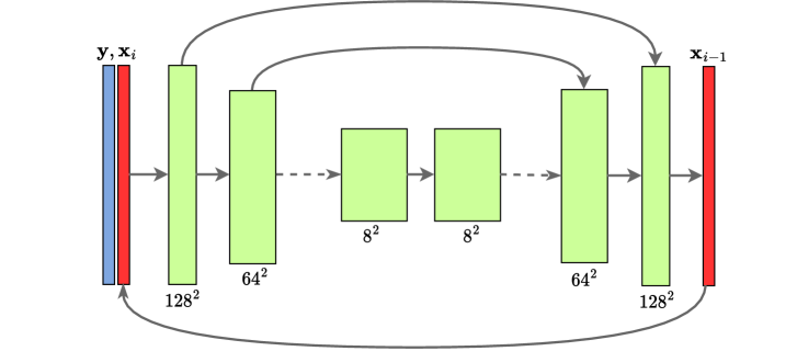
Figure 2: Architecture of the network. The concatenation of the low-resolution image $\mathbf{y}$ and the noisy image $\mathbf{x}_{i}$ is used as input to the network. Adapted from [13].

The source code and the network weights are publicly available at https://github.com/marcelowds/sr-sde.

III Experiments and Results

Here, we describe the proposed experiments and results obtained with our methods. In Section III-A we describe the main metrics used to verify the quality of the SR images. In Section III-B we describe how to use image features and cosine similarity CS to compare SR and HR images. We also analyze how the image smoothness can influence the PSNR and CS metrics. In Section III-C we demonstrate the superior quality of our method both qualitatively (with very detailed SR images) and quantitatively with the highest value for the CS metric, which is very important for recognition tasks. Finally, in Section III-D we describe the experimental parameters used in our experiments.

To evaluate the capacity of SDEs for the super-resolution task, the four algorithms SDE-VP, SDE-subVP, SDE-VE and SDE-VE cs are provided with $16\times 16$ images and produce $128\times 128$ images. The working size of the network is $128\times 128$, so the input is upsampled to this size.

III-A Super-resolution metrics and image smoothness

The metrics PSNR and SSIM are used to evaluate the quality of the SR images. We also use the consistency, defined as the Mean Squared Error (MSE) between the down-sampled SR images and the LR inputs. Aiming to evaluate the potential applications of our method on face recognition systems, we rely on the cosine similarity between the image features obtained from VGG-Face [20].

Specifically for the SDE-VE cs method, the Langevin correction depends on a parameter $r$ which controls the signal-to-noise ratio during the correction step. Higher values of $r$ typically result in smoother images, as can be seen in Fig. 3. It is well known that the PSNR and SSIM metrics are not adequate for measuring the quality of super-resolution images because these metrics tend to be very conservative with high-frequency details [26, 13]. Therefore, we use the SDE-VE cs algorithm to generate a set of images with different values of $r$ and analyze the influence of the smoothness level on the PSNR metric.

Original	Sample1	Sample2	Sample3

Figure 3: Samples obtained increasing $r$ from left to right. For Sample1, Sample2 and Sample3 the values of $r$ are $0.10$, $0.30$ and $0.52$ for the first row and $0.12$, $0.32$ and $0.39$ for the second row. Higher values of $r$ yield smoother images and larger values of PSNR (on average).

Fig. 4 shows PSNR as a function of the parameter $r$. As can be seen, higher values of $r$ cause the PSNR to increase, with the highest value of PSNR occurring at $r~{}\approx~{}0.5$. Thus, with smoother images, we can obtain higher values of PSNR. This is in line with the regression model of [13], which provides blurry and less detailed images than SR3, but with better results for PSNR and SSIM.

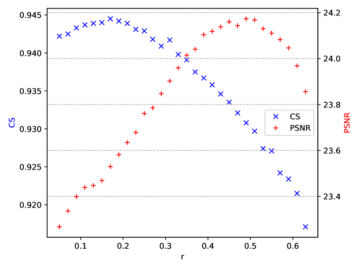
Figure 4: CS and PSNR as a function of $r$ (sampling parameter). Higher values of $r$ produce smoother images (with higher values of PSNR) but can decrease the value of CS.

III-B Feature extraction for face recognition

One application of super-resolution algorithms is face recognition. In real-world scenarios, the images of surveillance cameras are usually noisy and low resolution [27, 28, 29]. Hence, considering that our method is based on denoising, we believe it can be very suitable for such scenarios.

To evaluate the potential influence of the smoothness and PSNR metric on the recognition accuracy, we use different images obtained with the SDE-VE cs algorithm for different values of $r$, analyzing which of these images are better for the face recognition task. To compare the SR and HR images, we extract the features of the images using VGG-Face and measure the cosine similarity between them.

Let $\mathbf{x}$ and $\tilde{\mathbf{x}}$ be the super-resolved and the original images, respectively. The features extracted with VGG-Face is a one-dimensional vector of size $F$ and can be denoted by $\mathbf{z}=f(\mathbf{x})$ for the super-resolution images and $\tilde{\mathbf{z}}=f(\tilde{\mathbf{x}})$ for the original images; $f(\cdot)$ is a feature extractor function. The cosine similarity between these two vectors is computed using

$$s(\tilde{\mathbf{z}},\mathbf{z})=\frac{\langle\tilde{\mathbf{z}},\mathbf{z}\rangle}{\|\tilde{\mathbf{z}}\|\cdot\|\mathbf{z}\|},$$ (12)

where $\langle\cdot,\cdot\rangle$ denotes the scalar product, and $\|\cdot\|$ refers to the Euclidean norm. As the above similarity is calculated for $L$ images, we denote each feature vector by an index $i$. The average cosine similarity for the $L$ images, denoted by CS, is

$$\text{CS}=\frac{1}{L}\displaystyle\sum_{i=1}^{L}s(\tilde{\mathbf{z}}_{i},\mathbf{z}_{i}).$$ (13)

CS is the result of facial feature extraction, so it strongly influences recognition accuracy. CS values close to 1 indicate that the features of SR and HR images are very close and that the super-resolution algorithm is retrieving image details important for facial recognition.

As described in [26, 19], the PSNR metric does not align well with human perception. Now one may ask what are the best super-resolution images to use on the recognition tasks, for example, the images with high-frequency details (smaller values of $r$ and PSNR) or smoother images (higher values of $r$ and PSNR). To answer this question, we analyze CS, as a function of $r$ in Fig. 4. We observe that CS has a maximum value for $r~{}\approx~{}0.16$ (which is different from $r$ for which PSNR is maximum) and slightly decreases with $r$. We can also analyze if there is relation between the values of CS and PSNR, and for this purpose, we computed the correlation coefficient between CS and PSNR, obtaining a value of $-0.6591$. Therefore, not always higher values of PSNR are related to higher values of CS (and consequently higher recognition accuracy), as can be observed in the cross-plot between CS and PSNR in Fig. 5.

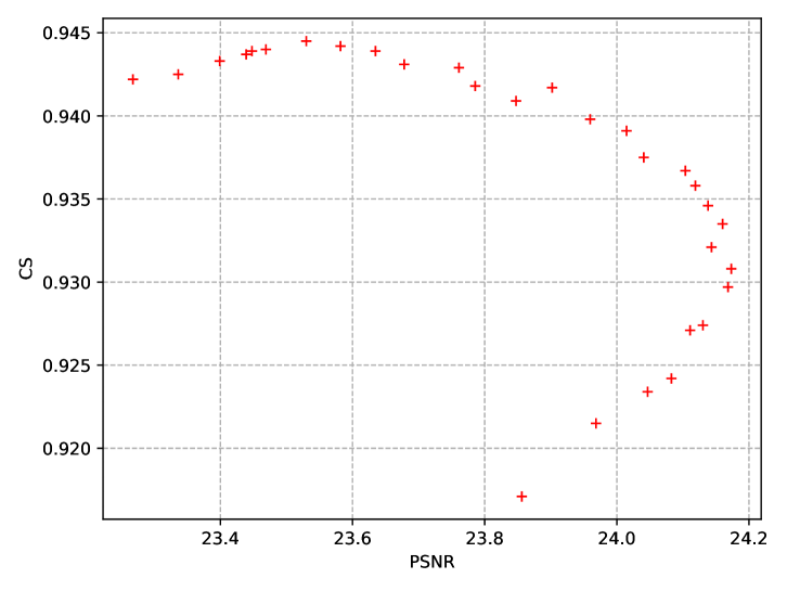
Figure 5: Cross-plot between CS and PSNR. The correlation coefficient between CS and PSNR is $-0.6591$, implying that higher values of PSNR do not always result in higher values of CS.

III-C Super-resolution

We evaluate the proposed methods qualitatively (visually) in Fig. 6, where it is demonstrated that the recovered images with SDE-VE have, in most cases, more quality, more high-frequency details, and are more natural when compared with other methods. The SPARNet method [30] generates images without distortion, but smoother when compared with our four methods. For some images, our SDE-VEcs method is able recover even the finest details, such as the beard in the image shown in the fifth row of Fig. 6.

Original	Input	GFP-GAN [31]i	SPARNet [30]	SR3 [13]	SDE-VP	SDE-subVP	SDE-VE	SDE-VEcs

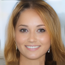
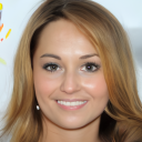
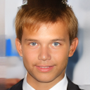
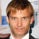
Figure 6: Super-resolution results. Our methods are shown in red (the best) and blue. SDE-VE provides more natural and detailed images than other methods. It is worth highlighting that SDE-VE cs can even retrieve finer details in some cases, such as the beard in the image shown in the fifth row.

TABLE I: PSNR, SSIM, Consistency and CS on $16\times 16\rightarrow 128\times 128$ face super-resolution. The best result for CS is highlighted with red.

Model	PSNR $\uparrow$	SSIM $\uparrow$	CONSISTENCY $\downarrow$	CS $\uparrow$
GFP-GAN [31]	$21.5326\pm 1.5273$	$0.6006\pm 0.0709$	$37.2256\pm 12.4622$	$0.8689\pm 0.0581$
SPARNet [30]	$25.2903\pm 1.9770$	$0.7526\pm 0.0676$	$\phantom{0}1.6826\pm\phantom{0}0.7652$	$0.9371\pm 0.0292$
SR3 [13]	$22.9581\pm 1.8370$	$0.6605\pm 0.0758$	$\phantom{0}1.3715\pm\phantom{0}0.7904$	$0.9370\pm 0.0244$
SDE-VP	$22.7171\pm 1.8107$	$0.6448\pm 0.0787$	$\phantom{0}0.1074\pm\phantom{0}0.0592$	$0.9330\pm 0.0262$
SDE-subVP	$22.6455\pm 1.8047$	$0.6428\pm 0.0797$	$\phantom{0}0.1433\pm\phantom{0}0.1212$	$0.9300\pm 0.0261$
SDE-VE	$23.5101\pm 1.9492$	$0.6879\pm 0.0797$	$\phantom{0}0.0454\pm\phantom{0}0.0357$	$0.9443\pm 0.0222$

To evaluate our results quantitatively, we present in Table I the metrics PSNR, SSIM, consistency and CS. The SPARNet method [30] achieves the highest value of PSNR and SSIM (these values may differ slightly from the original work due to slight differences in the dataset used). However, as discussed earlier, this is not enough to generate images with high-frequency details as it occurs in SR3 [13] and in the variations of the proposed approach. Considering that we intend to apply our super-resolution method to surveillance scenarios and facial recognition, we are interested in recovering details that maximize the CS metric. As shown in Table I, SDE-VE achieves the highest value for the CS metric, supporting the idea that the SDE-VE method performs better than other super-resolution methods for the face recognition task. When comparing our four methods based on SDEs presented here, the SDE-VE reached the best results.

III-D Parameters and network training

Following [15], we set the parameters of the models as $\sigma_{min}=0.01$, $\sigma_{max}=348$, $\bar{\beta}_{min}=0.1$, and $\bar{\beta}_{min}=20.0$. For the optimization, we used the Adam optimizer with a warm-up of $5000$ steps and a learning rate of $2\times 10^{-4}$.

For training, we explored the images from the Flickr-Faces-HQ (FFHQ) dataset [32] with $10^{6}$ steps. Low-quality images were obtained by downsampling the original high-resolution images by a factor of 8 and upsampling back to the original size using bicubic interpolation. For testing, considering the high execution time, we used a random sampling of $L=1024$ images of the CelebA-HQ dataset [33]. We perform our evaluation in a cross-dataset fashion because it provides a better indication of generalization (hence real-world performance) [34, 35]. Previous works also conducted experiments in this way [30, 13]. The total number of time steps was fixed in $N=2000$, and for the SDE-VE cs, we used $M=2$ correction steps. For the VGG-Face feature extraction, a feature vector size of $F=512$ was used.

All experiments were carried out on a computer with an AMD Ryzen $9$ $5950$X CPU ($3.4$GHz), $128$ GB of RAM ($2633$ MHz), and an NVIDIA Quadro RTX $8000$ GPU ($48$ GB).

IV Conclusions and future work

In this work, we presented an application in continuous time of diffusion models using SDEs. The diffusion models have been outperforming GANs for various sets of tasks and can train a model without instabilities (unlike GANs). When using facial features as metrics combined with qualitative analysis, we demonstrated that the SDE-VE model reaches better results than other methods for the super-resolution task.

The SDE-VE super-resolution algorithm also has excellent potential to be used for recognition tasks. As a next step, we intend to demonstrate the effectiveness of our method on images from surveillance camera datasets such as QUIS-CAMPI [36] and SCface [37].

The influence of the image smoothness and PSNR values on the recognition task will be further explored in future works. More specifically, explainability techniques can be used to analyze which characteristics change when we alter the image smoothness and PSNR values, similar to the work performed for periocular recognition in [38].

Despite the superior results of general diffusion models and the method presented in this work, which is based on SDEs, we remark that all these methods have a relatively high execution time. Thus, it is important to research novel strategies to improve the efficiency of these methods.

References

- [1] J. Sohl-Dickstein, E. Weiss, N. Maheswaranathan, and S. Ganguli, “Deep unsupervised learning using nonequilibrium thermodynamics,” in International Conference on Machine Learning, pp. 2256–2265, 2015.
- [2] J. Ho, A. Jain, and P. Abbeel, “Denoising diffusion probabilistic models,” in International Conference on Neural Information Processing Systems (NeurIPS), vol. 33, pp. 6840–6851, 2020.
- [3] Y. Song and S. Ermon, “Generative modeling by estimating gradients of the data distribution,” in International Conference on Neural Information Processing Systems (NeurIPS), pp. 1–13, 2019.
- [4] S. Särkkä and A. Solin, Applied stochastic differential equations, vol. 10. Cambridge University Press, 2019.
- [5] N. Chen, Y. Zhang, H. Zen, R. J. Weiss, M. Norouzi, and W. Chan, “Wavegrad: Estimating gradients for waveform generation,” arXiv preprint arXiv:2009.00713, 2020.
- [6] C. Niu et al., “Permutation invariant graph generation via score-based generative modeling,” in International Conference on Artificial Intelligence and Statistics (AISTATS), vol. 108, pp. 4474–4484, Aug 2020.
- [7] R. Cai, G. Yang, H. Averbuch-Elor, Z. Hao, S. Belongie, N. Snavely, and B. Hariharan, “Learning gradient fields for shape generation,” in European Conference on Computer Vision (ECCV), pp. 364–381, 2020.
- [8] P. Dhariwal and A. Nichol, “Diffusion models beat GANs on image synthesis,” in International Conference on Neural Information Processing Systems (NeurIPS), vol. 34, pp. 8780–8794, 2021.
- [9] C. Meng, Y. He, Y. Song, J. Song, J. Wu, J.-Y. Zhu, and S. Ermon, “SDEdit: Guided image synthesis and editing with stochastic differential equations,” in International Conf. on Learning Representations, 2022.
- [10] C. Saharia et al., “Photorealistic text-to-image diffusion models with deep language understanding,” arXiv preprint arXiv:2205.11487, 2022.
- [11] Y. Song, L. Shen, L. Xing, and S. Ermon, “Solving inverse problems in medical imaging with score-based generative models,” in International Conference on Learning Representations (ICLR), pp. 1–18, 2022.
- [12] B. Kawar, G. Vaksman, and M. Elad, “SNIPS: Solving noisy inverse problems stochastically,” in International Conference on Neural Information Processing Systems (NeurIPS), pp. 21 757–21 769, 2021.
- [13] C. Saharia, J. Ho, W. Chan, T. Salimans, D. J. Fleet, and M. Norouzi, “Image super-resolution via iterative refinement,” arXiv preprint, vol. arXiv:2104.07636, pp. 1–28, 2021, Google Research.
- [14] H. Li, Y. Yang, M. Chang, S. Chen, H. Feng, Z. Xu, Q. Li, and Y. Chen, “SRDiff: Single image super-resolution with diffusion probabilistic models,” Neurocomputing, vol. 479, pp. 47–59, 2022.
- [15] Y. Song et al., “Score-based generative modeling through stochastic differential equations,” in International Conference on Learning Representations (ICLR), pp. 1–36, May 2021.
- [16] A. Jolicoeur-Martineau, K. Li, R. Piché-Taillefer, T. Kachman, and I. Mitliagkas, “Gotta go fast when generating data with score-based models,” arXiv preprint arXiv:2105.14080, 2021.
- [17] A. Vahdat, K. Kreis, and J. Kautz, “Score-based generative modeling in latent space,” in International Conference on Neural Information Processing Systems (NeurIPS), vol. 34, pp. 11 287–11 302, 2021.
- [18] T. Dockhorn, A. Vahdat, and K. Kreis, “Score-based generative modeling with critically-damped langevin diffusion,” in International Conference on Learning Representations (ICLR), pp. 1–54, 2022.
- [19] R. Zhang et al., “The unreasonable effectiveness of deep features as a perceptual metric,” in IEEE/CVF Conference on Computer Vision and Pattern Recognition (CVPR), pp. 586–595, 2018.
- [20] Oxford VGGFace Implementation using Keras Functional Framework v2+. [Online]. Available: https://github.com/rcmalli/keras-vggface
- [21] P. Kloeden and E. Platen, The Numerical Solution of Stochastic Differential Equations, vol. 23. Springer, Jan 2011.
- [22] B. D. Anderson, “Reverse-time diffusion equation models,” Stochastic Processes and their Applications, vol. 12, no. 3, pp. 313–326, 1982.
- [23] P. Vincent, “A connection between score matching and denoising autoencoders,” Neural computation, vol. 23, no. 7, pp. 1661–1674, 2011.
- [24] G. Parisi, “Correlation functions and computer simulations,” Nuclear Physics B, vol. 180, no. 3, pp. 378–384, 1981.
- [25] R. M. Neal et al., “Mcmc using hamiltonian dynamics,” Handbook of markov chain monte carlo, vol. 2, no. 11, p. 2, 2011.
- [26] J. Johnson, A. Alahi, and L. Fei-Fei, “Perceptual losses for real-time style transfer and super-resolution,” in European Conference on Computer Vision (ECCV), pp. 694–711, 2016.
- [27] R. Abiantun, F. Juefei-Xu, U. Prabhu, and M. Savvides, “SSR2: Sparse signal recovery for single-image super-resolution on faces with extreme low resolutions,” Pattern Recognition, vol. 90, pp. 308–324, 2019.
- [28] P. Li, L. Prieto, D. Mery, and P. J. Flynn, “On low-resolution face recognition in the wild: Comparisons and new techniques,” IEEE Transactions on Information Forensics and Security, vol. 14, pp. 2000–2012, 2019.
- [29] G. R. Gonçalves et al., “Multi-task learning for low-resolution license plate recognition,” in Iberoamerican Congress on Pattern Recognition (CIARP), pp. 251–261, Oct 2019.
- [30] C. Chen, D. Gong, H. Wang, Z. Li, and K.-Y. K. Wong, “Learning spatial attention for face super-resolution,” IEEE Transactions on Image Processing, vol. 30, pp. 1219–1231, 2020.
- [31] X. Wang, Y. Li, H. Zhang, and Y. Shan, “Towards real-world blind face restoration with generative facial prior,” in IEEE/CVF Conference on Computer Vision and Pattern Recognition, pp. 9164–9174, 2021.
- [32] T. Karras, S. Laine, and T. Aila, “A style-based generator architecture for generative adversarial networks,” in IEEE/CVF Conference on Computer Vision and Pattern Recognition (CVPR), pp. 4396–4405, 2019.
- [33] T. Karras, T. Aila, S. Laine, and J. Lehtinen, “Progressive growing of GANs for improved quality, stability, and variation,” in International Conference on Learning Representations (ICLR), pp. 1–26, 2018.
- [34] A. Torralba and A. A. Efros, “Unbiased look at dataset bias,” in IEEE/CVF Conference on Computer Vision and Pattern Recognition (CVPR), pp. 1521–1528, June 2011.
- [35] R. Laroca, M. Santos, V. Estevam, E. Luz, and D. Menotti, “A first look at dataset bias in license plate recognition,” arXiv preprint, vol. arXiv:2208.10657, pp. 1–6, 2022.
- [36] J. Neves, J. Moreno, and H. Proença, “QUIS-CAMPI: an annotated multi-biometrics data feed from surveillance scenarios,” IET Biometrics, vol. 7, no. 4, pp. 371–379, 2018.
- [37] M. Grgic, K. Delac, and S. Grgic, “SCface – surveillance cameras face database,” Multimedia tools and applications, vol. 51, no. 3, pp. 863–879, 2011.
- [38] J. Brito and H. Proença, “A short survey on machine learning explainability: An application to periocular recognition,” Electronics, vol. 10, no. 15, p. 1861, 2021.