Non-monotonic Resource Utilization in the Bandits with Knapsacks Problem

Abstract

Bandits with knapsacks ($\mathsf{BwK}$) [6] is an influential model of sequential decision-making under uncertainty that incorporates resource consumption constraints. In each round, the decision-maker observes an outcome consisting of a reward and a vector of nonnegative resource consumptions, and the budget of each resource is decremented by its consumption. In this paper we introduce a natural generalization of the stochastic $\mathsf{BwK}$ problem that allows non-monotonic resource utilization. In each round, the decision-maker observes an outcome consisting of a reward and a vector of resource drifts that can be positive, negative or zero, and the budget of each resource is incremented by its drift. Our main result is a Markov decision process (MDP) policy that has constant regret against a linear programming (LP) relaxation when the decision-maker knows the true outcome distributions. We build upon this to develop a learning algorithm that has logarithmic regret against the same LP relaxation when the decision-maker does not know the true outcome distributions. We also present a reduction from $\mathsf{BwK}$ to our model that shows our regret bound matches existing results [14].

1 Introduction

Multi-armed bandits are the quintessential model of sequential decision-making under uncertainty in which the decision-maker must trade-off between exploration and exploitation. They have been studied extensively and have numerous applications, such as clinical trials, ad placements, and dynamic pricing to name a few. We refer the reader to Bubeck and Cesa-Bianchi [7], Slivkins [17], Lattimore and Szepesvári [13] for an introduction to bandits. An important shortcoming of the basic stochastic bandits model is that it does not take into account resource consumption constraints that are present in many of the motivating applications. For example, in a dynamic pricing application the seller may be constrained by a limited inventory of items that can run out well before the end of the time horizon. The bandits with knapsacks $(\mathsf{BwK}$) model [18, 19, 5, 6] remedies this by endowing the decision-maker with some initial budget for each of $m$ resources. In each round, the outcome is a reward and a vector of nonnegative resource consumptions, and the budget of each resource is decremented by its consumption. The process ends when the budget of any resource becomes nonpositive. However, even this formulation fails to model that in many applications resources can get replenished or renewed over time. For example, in a dynamic pricing application a seller may receive shipments that increase their inventory level.

Contributions

In this paper we introduce a natural generalization of $\mathsf{BwK}$ by allowing non-monotonic resource utilization. The decision-maker starts with some initial budget for each of $m$ resources. In each round, the outcome is a reward and a vector of resource drifts that can be positive, negative or zero, and the budget of each resource is incremented by its drift. A negative drift has the effect of decreasing the budget akin to consumption in $\mathsf{BwK}$ and a positive drift has the effect of increasing the budget. We consider two settings: (i) when the decision-maker knows the true outcome distributions and must design a Markov decision process (MDP) policy; and (ii) when the decision-maker does not know the true outcome distributions and must design a learning algorithm.

Our main contribution is an MDP policy, ControlBudget(CB), that has constant regret against a linear programming (LP) relaxation. Such a result was not known even for $\mathsf{BwK}$. We build upon this to develop a learning algorithm, ExploreThenControlBudget(ETCB), that has logarithmic regret against the same LP relaxation. We also present a reduction from $\mathsf{BwK}$ to our model and show that our regret bound matches existing results.

Instead of merely sampling from the optimal probability distribution over arms, our policy samples from a perturbed distribution to ensure that the budget of each resource stays close to a decreasing sequence of thresholds. The sequence is chosen such that the expected leftover budget is a constant and proving this is a key step in the regret analysis. Our work combines aspects of related work on logarithmic regret for $\mathsf{BwK}$ [9, 14].

Related Work

Multi-armed bandits have a rich history and logarithmic instance-dependent regret bounds have been known for a long time [12, 3]. Since then, there have been numerous papers extending the stochastic bandits model in a variety of ways [4, 16, 11, 6, 10, 2, 1].

To the best of our knowledge, there are three papers on logarithmic regret bounds for $\mathsf{BwK}$. Flajolet and Jaillet [9] showed the first logarithmic regret bound for $\mathsf{BwK}$. In each round, their algorithm finds the optimal basis for an optimistic version of the LP relaxation, and chooses arms from the resulting basis to ensure that the average resource consumption stays close to a pre-specified level. Even though their regret bound is logarithmic in $T$ and inverse linear in the suboptimality gap, it is exponential in the number of resources. Li et al. [14] showed an improved logarithmic regret bound that is polynomial in the number of resources, but it scales inverse quadratically with the suboptimality gap and their definition of the gap is different from the one in Flajolet and Jaillet [9]. The main idea behind improving the dependence on the number of resources is to proceed in two phases: (i) identify the set of arms and binding resources in the optimal solution; (ii) in each round, solve an adaptive, optimistic version of the LP relaxation and sample an arm from the resulting probability distribution. Finally, Sankararaman and Slivkins [15] show a logarithmic regret bound for $\mathsf{BwK}$ against a fixed-distribution benchmark. However, the regret of this benchmark itself with the optimal MDP policy can be as large as $O(\sqrt{T})$ [9, 14].

2 Preliminaries

2.1 Model

Let $T$ denote a finite time horizon, ${\cal X}=\{1,\dots,k\}$ a set of $k$ arms, ${\cal J}=\{1,\dots,m\}$ denote a set of $m$ resources, and $B_{0,j}=B$ denote the initial budget of resource $j$. In each round $t\in[T]$, if the budget of any resource is less than $1$, then ${\cal X}_{t}=\{1\}$. Otherwise, ${\cal X}_{t}={\cal X}$. The algorithm chooses an arm $x_{t}\in{\cal X}_{t}$ and observes an outcome $o_{t}=(r_{t},d_{t,1},\dots,d_{t,m})\in[0,1]\times[-1,1]^{m}$. The algorithm earns reward $r_{t}$ and the budget of resource $j\in{\cal J}$ is incremented by drift $d_{t,j}$ as $B_{t,j}=B_{t-1,j}+d_{t,j}$.

Each arm $x\in{\cal X}$ has an outcome distribution over $[0,1]\times[-1,1]^{m}$ and $o_{t}$ is drawn from the outcome distribution of the arm $x_{t}$. We use $\mu_{x}^{o}=(\mu_{x}^{r},\mu_{x}^{d,1},\dots,\mu_{x}^{d,m})$ to denote the expected outcome vector of arm $x$ consisting of the expected reward and the expected drifts for each of the $m$ resources. We also use $\mu^{d,j}=(\mu_{x}^{d,j}:x\in{\cal X})$ to denote the vector of expected drifts for resource $j$. We assume that arm $x^{0}=1\in{\cal X}$ is a null arm with three important properties: (i) its reward is zero a.s.; (ii) the drift for each resource is nonnegative a.s.; and (iii) the expected drift for each resource is positive. The second and third properties of the null arm plus the model’s requirement that $x_{t}=1$ if $\exists j$ s.t. $B_{t-1,j}<1$ ensure that the budgets are nonnegative a.s. and can be safely increased from $0$.

Our model is intended to capture applications featuring resource renewal, such as the following. In each round, each resource gets replenished by some random amount and the chosen arm consumes some random amount of each resource. If the consumption is less than replenishment, the resource gets renewed. The random variable $d_{t,j}$ then models the net replenishment minus consumption. The full model presented above is more general because it allows both the consumption and replenishment to depend on the arm pulled.

We consider two settings in this paper.

MDP setting

The decision-maker knows the true outcome distributions. In this setting the model implicitly defines an MDP, where the state is the budget vector, the actions are arms, and the transition probabilities are defined by the outcome distributions of the arms.

Learning setting

The decision-maker does not know the true outcome distributions.

The goal is to design to an MDP policy for the first setting and a learning algorithm for the second, and bound their regret against an LP relaxation as defined in the next subsection.

2.2 Linear Programming Relaxation

Similar to Badanidiyuru et al. [6, Lemma 3.1], we consider the following LP relaxation that provides an upper bound on the total expected reward of any algorithm:

$$\mathsf{OPT}_{\mathsf{LP}}=\max_{p}\left\{\sum_{x\in{\cal X}}p_{x}\mu_{x}^{r}:\sum_{x\in{\cal X}}p_{x}\mu_{x}^{d,j}\geq\nicefrac{{-B}}{{T}}\ \forall j\in{\cal J},\ \sum_{x\in{\cal X}}p_{x}=1,\ p_{x}\geq 0\ \forall x\in{\cal X}\right\}.$$ (1)

Lemma 2.1.

The total expected reward of any algorithm is at most $T\cdot\mathsf{OPT}_{\mathsf{LP}}$.

The proof of this lemma, similar to those in existing works [2, 6], follows from the observations that (i) the variables $p=\{p_{x}:x\in{\cal X}\}$ can be interpreted as the probability of choosing arm $x$ in a round; and (ii) if we set $p_{x}$ equal to the expected number of times $x$ is chosen by an algorithm divided by $T$, then it is a feasible solution for the LP.

Definition 2.1 (Regret).

The regret of an algorithm ${\cal A}$ is defined as $R_{T}({\cal A})=T\cdot\mathsf{OPT}_{\mathsf{LP}}-\mathsf{REW}({\cal A})$, where $\mathsf{REW}({\cal A})$ denotes the total expected reward of ${\cal A}$.

2.3 Assumptions

We assume that the initial budget of every resource is $B\leq T$. This assumption is without loss of generality because otherwise we can scale the drifts by dividing them by the smallest budget. This results in a smaller support set for the drift distribution that is still contained in $[-1,1]$.

Our assumptions about the null arm $x^{0}$ are a major difference between our model and $\mathsf{BwK}$. In $\mathsf{BwK}$ the budgets can only decrease and the process ends when the budget of any resource reaches $0$. However, in our model the budgets can increase or decrease, and the process ends at the end of the time horizon. Our assumptions about the null arm allow us to increase the budget from $0$ without making it negative. A side-effect of this is that in our model we can even assume that $B$ is a small constant because we can always increase the budget by pulling the null arm, in contrast to existing literature on $\mathsf{BwK}$ that assume the initial budgets are large and often scale with the time horizon.

A standard assumption for achieving logarithmic regret in stochastic bandits is that the gap between the total expected reward of an optimal arm and that of a second-best arm is positive. There are a few different ways in which one could translate this to our model where the optimal solution is a mixture over arms. We make the following choice. We assume that there exists a unique set of arms $X^{*}$ that form the support set of the LP solution and a unique set of resources $J^{*}$ that correspond to binding constraints in the LP solution [14]. We define the gap of the problem instance in Definition 4.1 and our uniqueness assumption implies that the gap is strictly positive.

We make a few separation assumptions parameterized by four positive constants that can be arbitrarily small. First, the smallest magnitude of the drifts, $\delta_{\text{drift}}=\min\{|\mu_{x}^{d,j}|:x\in{\cal X},j\in{\cal J}\}$, satisfies $\delta_{\text{drift}}>0$. Second, the smallest singular value of the LP constraint matrix, denoted by $\sigma_{\min}$, satisfies $0<\sigma_{\min}<1$. Third, the LP solution $p^{*}$ satisfies $p^{*}_{x}\geq\delta_{\text{support}}>0$ for all $x\in X^{*}$. Fourth, $\sum_{x\in X^{*}}p^{*}_{x}\mu_{x}^{d,j}\geq\delta_{\text{slack}}>0$ for all resources $j\notin J^{*}$. The first assumption is necessary for logarithmic regret bounds because otherwise one can show that the regret of the optimal algorithm for the case of one resoure and one zero-drift arm is $\Theta(\sqrt{T})$ (Appendix B). The second and third assumptions are essentially the same as in existing literature on logarithmic regret bounds for $\mathsf{BwK}$ [9, 14]. The fourth assumption allows us to design algorithms that can increase the budgets of the non-binding resources away from $0$, thereby reducing the number of times the algorithm has to pull the null arm. Otherwise, if they have zero drift, then, as stated above, the regret of the optimal algorithm for the case of one resource and one zero-drift arm is $\Theta(\sqrt{T})$ (Appendix B).

3 MDP Policy with Constant Regret

In this section we design an MDP policy, ControlBudget (Algorithm 2), with constant regret in terms of $T$ for the setting when the learner knows the true outcome distributions and our model implicitly defines an MDP (Section 2.1). At a high level, ControlBudget, which shares similarities with Flajolet and Jaillet [9, Algorithm UCB-Simplex], plays arms to keep the budgets close to a decreasing sequence of thresholds. The choice of this sequence allows us to show that the expected leftover budgets and the expected number of null arm pulls are constants. This is a key step in proving the final regret bound. We start by considering the special case of one resource in Section 3.1 because it provides intuition for the general case of multiple resources in Section 3.2.

3.1 Special Case: One Resource

Since there is only one resource we drop the superscript $j$ in this section. We say that an arm $x$ is a positive (resp. negative) drift arm if $\mu_{x}^{d}>0$ (resp. $\mu_{x}^{d}<0$). The following lemma characterizes the possible solutions of the LP (Eq. 1).

Lemma 3.1.

The solution of the LP relaxation (Eq. 1) is supported on at most two arms. Furthermore, if $T\geq\nicefrac{{B}}{{\delta_{\text{drift}}}}$, then the solution belongs to one of three categories: (i) supported on a single positive drift arm; (ii) supported on the null arm and a negative drift arm; (iii) supported on a positive drift arm and a negative drift arm.

The proof of this lemma follows from properties of LPs and a case analysis of which constraints are tight. Our MDP policy, ControlBudget (Algorithm 1), deals with the three cases separately and satisfies the following regret bound.

Input: time horizon $T$, initial budget $B$, set of arms ${\cal X}$, set of resources ${\cal J}$, constant $c>0$.

1

2Set $B_{0}=B$.

3if LP solution is supported on positive drift arm $x^{p}$ then

4      

5      for $t=1,2,\dots,T$ do

6            

7            If $B_{t-1}<1$, pull $x^{0}$. Otherwise, pull $x^{p}$.

8       end for

9      

10 else if LP solution is supported on null arm $x^{0}$ and negative drift arm $x^{n}$ then

11      

12      for $t=1,2,\dots,T$ do

13            

14            Define threshold $\tau_{t}=c\log(T-t)$.

15            If $B_{t-1}<\max\{1,\tau_{t}\}$, pull $x^{0}$. Otherwise, pull $x^{n}$.

16       end for

17      

18 else if LP solution is supported on positive drift arm $x^{p}$ and negative drift arm $x^{n}$ then

19      

20      for $t=1,2,\dots,T$ do

21            

22            Define threshold $\tau_{t}=c\log(T-t)$.

23            If $B_{t-1}<1$, pull $x^{0}$. If $1\leq B_{t-1}<\tau_{t}$, pull $x^{p}$. Otherwise, pull $x^{n}$.

24       end for

25      

Algorithm 1 ControlBudget (for $m=1$)

Theorem 3.1.

If $c\geq\frac{6}{\delta_{\text{drift}}^{2}}$, the MDP policy ControlBudget (Algorithm 1) satisfies

$$R_{T}(\texttt{ControlBudget})\leq\tilde{C},$$ (2)

where $\tilde{C}=O\left(\delta_{\text{drift}}^{-4}\ln\left(\left(1-\exp\left(-\frac{\delta_{\text{drift}}^{2}}{8}\right)\right)^{-1}\right)+\delta_{\text{drift}}^{-1}\left(1-\exp\left(\delta_{\text{drift}}^{2}\right)\right)^{-2}\right)$ is a constant.

We defer all proofs in this section to Appendix C, but we include a proof sketch of most results in the main paper following the statement. The proof of Theorem 3.1 follows from the following sequence of lemmas.

Lemma 3.2.

If the LP solution is supported on a positive drift arm $x^{p}$, then

$$R_{T}(\texttt{ControlBudget})\leq\tilde{C},$$ (3)

where $\tilde{C}=O\left(\delta_{\text{drift}}^{-3}\ln\left(\left(1-\exp\left(-\frac{\delta_{\text{drift}}^{2}}{8}\right)\right)^{-1}\right)\right)$ is a constant.

We can write the regret in terms of the norm of $\xi=(\xi_{x^{p}})$, where $\xi_{x^{p}}$ is the expected difference between the number of times $x^{p}$ is played by the LP and by ControlBudget. This is equal to the expected number of times the policy plays the null arm and, in turn, is equal to the expected number of rounds in which the budget is below $1$. Since both $x^{0}$ and $x^{p}$ have positive drift, this is a transient random walk that drifts away from $0$. It is known that such a walk spends a constant number of rounds in any state in expectation.

Lemma 3.3.

If the LP solution is supported on the null arm $x^{0}$ and a negative drift arm $x^{n}$, then

$$R_{T}(\texttt{ControlBudget})\leq\tilde{C}\cdot\mathbb{E}[B_{T}],$$ (4)

where $\tilde{C}=O(\delta_{\text{drift}}^{-1})$ is a constant.

We can write the regret in terms of the norm of $\xi=(\xi_{x^{0}},\xi_{x^{n}})$, where $\xi_{x}$ is the expected difference between the number of times $x$ is played by the LP and by ControlBudget. Since both constraints (resource and sum-to-one) are tight, the lemma follows by writing $\xi=D^{-1}b$ and taking norms, where $D$ is the LP constraint matrix and $b=(-\mathbb{E}[B_{T}],0)$.

Lemma 3.4.

If the LP solution is supported on a positive drift arm $x^{p}$ and a negative drift arm $x^{n}$, then

$$R_{T}(\texttt{ControlBudget})\leq\tilde{C}\cdot\max\{\mathbb{E}[B_{T}],\mathbb{E}[N_{x^{0}}]\},$$ (5)

where $\mathbb{E}[N_{x^{0}}]$ denotes the expected number null arm pulls and $\tilde{C}=O(\delta_{\text{drift}}^{-1})$ is a constant.

This lemma follows similarly to the previous one by writing regret in terms of the norm of $\xi=(\xi_{x^{p}},\xi_{x^{n}})$ and writing $\xi=D^{-1}b$ for $b=(-\mathbb{E}[B_{T}],\mathbb{E}[N_{x^{0}}])$.

Therefore, proving that $R_{T}(\texttt{ControlBudget})$ is a constant in $T$ requires proving that both the expected leftover budget and expected number of null arm pulls are constants. Intuitively, we could ensure $\mathbb{E}[B_{T}]$ is small by playing the negative drift arm whenever the budget is at least $1$. However, there is constant probability of the budget decreasing below $1$ and the expected number of null arm pulls becomes $O(T)$. ControlBudget solves the tension between the two objectives by carefully choosing a decreasing sequence of thresholds $\tau_{t}$. The threshold is initially far from $0$ to ensure low probability of pre-mature resource depletion, but decreases to $0$ over time to ensure small expected leftover budget and decreases at a rate that ensures the expected number of null arm pulls is a constant.

Lemma 3.5.

If the LP solution is supported on a positive drift arm $x^{p}$ and a negative drift arm $x^{n}$, and $c\geq\frac{6}{\delta_{\text{drift}}^{2}}$, then

$$\mathbb{E}[N_{x^{0}}]\leq\tilde{C},$$ (6)

where $\tilde{C}=O\left(\delta_{\text{drift}}^{-3}\ln\left(\left((1-\exp\left(-\frac{\delta_{\text{drift}}^{2}}{8}\right)\right)^{-1}\right)\right)$ is a constant.

If the budget is below the threshold, i.e., $B_{t-1}<\tau_{t}$ for some $t$, then ControlBudget pulls $x^{p}$ until $B_{s}\geq\tau_{s+1}$ for some $s\geq t$. Since $x^{p}$ has positive drift, the event that repeated pulls decrease the budget towards $0$ is a low probability event. Using this, our choice of $\tau_{t}=c\log(T-t)$ for an appropriate constant $c$, and summing over all rounds shows that the expected number of rounds in which the budget is less than $1$ is a constant in $T$.

Lemma 3.6.

If the LP solution is supported on two arms, and $c\geq\frac{6}{\delta_{\text{drift}}^{2}}$, then

$$\mathbb{E}[B_{T}]\leq\tilde{C},$$ (7)

where $\tilde{C}=\tilde{O}\left(\left(1-\exp\left(\delta_{\text{drift}}^{2}\right)\right)^{-2}+\delta_{\text{drift}}^{-2}\right)$ is a constant.

If $B_{t-1}\geq\tau_{t}$, then ControlBudget pulls a negative drift arm $x^{n}$. We can upper bound the expected leftover budget by conditioning on $q$, the number of consecutive pulls of $x^{n}$ at the end of the timeline. The main idea in completing the proof is that (i) if $q$ is large, then it corresponds to a low probability event; and (ii) if $q$ is small, then the budget in round $T-q$ was smaller than $\tau_{q}$, which is a decreasing sequence in $q$, and there are few rounds left so the budget cannot increase by too much.

3.2 General Case: Multiple Resources

Now we use the ideas from Section 3.1 to tackle the case of $m>1$ resources that is much more challenging. Generalizing Lemma 3.1, the solution of the LP relaxation (Eq. 1) is supported on at most $\min\{k,m\}$ arms. Informally, our MDP policy, ControlBudget (Algorithm 2), samples an arm from a probability distribution that ensures drifts bounded away from $0$ in the “correct directions”: (i) a binding resource $j$ has drift at least $\gamma_{t}$ if $B_{t-1,j}<\tau_{t}$ and drift at most $-\gamma_{t}$ if $B_{t-1,j}\geq\tau_{t}$; and (ii) a non-binding resource $j$ has drift at least $\frac{1}{2}\gamma_{t}$ if $B_{t-1,j}<\tau_{t}$. This allows us to show that the expected leftover budget for each binding resource and the expected number of null arm pulls are constants in terms of $T$.

Input: time horizon $T$, initial budget $B$, set of arms ${\cal X}$, set of resources ${\cal J}$, constant $c>0$.

1

2Set $B_{0,j}=B$ for all $j\in{\cal J}$.

3Define threshold $\tau_{t}=c\log(T-t)$.

4for $t=1,2,\dots,T$ do

5      

6      if $\exists j\in{\cal J}$ such that $B_{t-1,j}<1$ then

7             Pull the null arm $x^{0}$.

8       else

9             Define $s_{t}\in\{\pm 1\}^{|X^{*}|-1}\times 0$ as follows. Let $j$ denote the resource corresponding to row $i\in[|X^{*}|-1]$ in the matrix $D$ and vector $b$. Then, the $i$th entry of $s_{t}$ is $+1$ if $B_{t-1,j}<\tau_{t}$ and $-1$ otherwise.

10            Define $\gamma_{t}$ to be the solution to the following constrained optimization problem:

$$\max_{\gamma\in[0,1]}\left\{\gamma:p=D^{-1}(b+\gamma s_{t})\geq 0,\ p^{T}\mu^{d,j}\geq\frac{\gamma}{2}\ \forall j\in{\cal J}\setminus J^{*}\text{ if }B_{t-1,j}<\tau_{t}\right\}.$$ (8)

11            Sample an arm from the probability distribution $p_{t}=D^{-1}(b+\gamma_{t}s_{t})$.

12       end if

13      

14 end for

Algorithm 2 ControlBudget (for general $m$)

Theorem 3.2.

If $c\geq\frac{6}{\gamma^{*2}}$, the regret of ControlBudget (Algorithm 2) satisfies

$$R_{T}(\texttt{ControlBudget})\leq\tilde{C},$$ (9)

where $\gamma^{*}$ (defined in Lemma 3.9) and $\tilde{C}$ are constants with $\tilde{C}=O\left(m\sigma_{\min}^{-1}\left(m(\gamma^{*})^{-3}\ln\left(\left((1-\exp\left(-\gamma^{*2}\right)\right)^{-1}\right)+\left(1-\exp(\gamma^{*2})\right)^{-2}\right)\right)$.

We defer all proofs in this section to Appendix D, but we include a proof sketch of most results in the main paper following the statement. The proof of Theorem 3.2 follows from the following sequence of lemmas. The next two lemmas are generalizations of Lemmas 3.3 and 3.4 with essentially the same proofs. Recall $J^{*}$ denotes the unique set of resources that correspond to binding constraints in the LP solution (Section 2.3).

Lemma 3.7.

If the LP solution includes the null arm $x^{0}$ in its support, then

$$R_{T}(\texttt{ControlBudget})\leq\tilde{C}\cdot\left(\sum_{j\in J^{*}}\mathbb{E}[B_{T,j}]\right),$$ (10)

where $\tilde{C}=O(\sigma_{\min}^{-1})$ is a constant.

Lemma 3.8.

If the LP solution does not include the null arm $x^{0}$ in its support, then

$$R_{T}(\texttt{ControlBudget})\leq\tilde{C}\cdot\left(\sum_{j\in J^{*}}\mathbb{E}[B_{T,j}]+\mathbb{E}[N_{x^{0}}]\right),$$ (11)

where $\mathbb{E}[N_{x^{0}}]$ denotes the expected number of null arm pulls and $\tilde{C}=O(\sigma_{\min}^{-1})$ is a constant.

Lemmas 3.10 and 3.11 are generalizations of Lemmas 3.5 and 3.6 with similar proofs after taking a union bound over resources. But we first need Lemma 3.9 that lets us conclude there is drift of magnitude at least $\gamma^{*}>0$ in the “correct directions” as stated earlier.

Lemma 3.9.

[9, Lemma 14] In each round $t$, $\gamma_{t}\geq\gamma^{*}=\frac{\sigma_{\min}\min\{\delta_{\text{support}},\delta_{\text{slack}}\}}{4m}$.

The proof of this lemma is identical to Flajolet and Jaillet [9, Lemma 14] but we provide a proof in the appendix for completeness.

Lemma 3.10.

If the LP solution does not include the null arm in its support, then

$$\mathbb{E}[N_{x^{0}}]\leq\tilde{C},$$ (12)

where $\tilde{C}=O\left(m(\gamma^{*})^{-3}\ln\left(\left((1-\exp\left(-\frac{\gamma^{*2}}{8}\right)\right)^{-1}\right)\right)$ is a constant.

Lemma 3.11.

If the LP solution is supported on more than one arm, then for all $j\in J^{*}$

$$\mathbb{E}[B_{T,j}]\leq\tilde{C},$$ (13)

where $\tilde{C}=\tilde{O}\left(\left(1-\exp(\gamma^{*2})\right)^{-2}+(\gamma^{*})^{-2}\right)$ is a constant.

A subtle but important point is that the regret analysis does not require ControlBudget to know the true expected drifts in order to find the probability vector $p_{t}$. It simply requires the algorithm to know $X^{*}$, $J^{*}$, and find any probability vector $p_{t}$ that ensures drifts bounded away from $0$ in the “correct directions” as stated earlier. We use this property in our learning algorithm, ExploreThenControlBudget (Algorithm 3), in the next section.

4 Learning Algorithm with Logarithmic Regret

In this section we design a learning algorithm, ExploreThenControlBudget (Algorithm 3), with logarithmic regret in terms of $T$ for the setting when the learning does not know the true distributions. Our algorithm, which can be viewed as combining aspects of Li et al. [14, Algorithm 1] and Flajolet and Jaillet [9, Algorithm UCB-Simplex], proceeds in three phases. It uses phase one of Li et al. [14, Algorithm 1] to identify the set of optimal arms $X^{*}$ and the set of binding constraints $J^{*}$ by playing arms in a round-robin fashion, and using confidence intervals and properties of LPs. This is reminiscent of successive elimination [8], except that the algorithm tries to identify the optimal arms instead of eliminating suboptimal ones. In the second phase the algorithm continues playing the arms in $X^{*}$ in a round-robin fashion to shrink the confidence radius further. In the third phase the algorithm plays a variant of the MDP policy ControlBudget (Algorithm 2) with a slighly different optimization problem for $\gamma_{t}$ because it only has empirical esitmates of the drifts.

4.1 Additional Notation and Preliminaries

For all arms $x\in{\cal X}$ and rounds $t\geq k$, define the upper confidence bound (UCB) of the expected outcome vector $\mu_{x}^{o}$ as $\mathsf{UCB}_{t}(x)=\bar{o}_{t}(x)+\mathsf{rad}_{t}(x)$, where $\mathsf{rad}_{t}(x)=\sqrt{8n_{t}(x)^{-1}\log T}$ denotes the confidence radius, $n_{t}(x)$ denotes the number of times $x$ has been played before $t$, and $\bar{o}_{t}(x)=n_{t}(x)^{-1}\sum_{t}o_{t}\mathbbm{1}[x_{t}=x]$ denotes the empirical mean outcome vector of $x$. The lower confidence bound (LCB) is defined similarly as $\mathsf{LCB}_{t}(x)=\bar{o}_{t}(x)-\mathsf{rad}_{t}(x)$.

For all arms $x\in{\cal X}$, let $\mathsf{OPT}_{-x}$ denote the value of the LP relaxation (Eq. 1) with the additional constraint $p_{x}=0$, and for all resources $j\in{\cal J}$, let $\mathsf{OPT}_{-j}$ denote the value when the objective has an extra $-\sum_{x}p_{x}\mu_{x}^{d,j}+\nicefrac{{B}}{{T}}$ term [14]. Intuitively, these represent how important it is to play arm $x$ or make the resource constraint for $j$ a binding constraint. Define the UCB of $\mathsf{OPT}_{-x}$ to be the value of the LP when the expected outcome is replaced by its UCB, and denote this by $\mathsf{UCB}_{t}(\mathsf{OPT}_{-x})$. The LCB for $\mathsf{OPT}_{-x}$, and UCB and LCB for $\mathsf{OPT}_{-j}$ and $\mathsf{OPT}_{\mathsf{LP}}$ are defined similarly.

Definition 4.1 (Gap [14]).

The gap of the problem instance is defined as

$$\Delta=\min\left\{\min_{x\in X^{*}}\left\{\mathsf{OPT}_{\mathsf{LP}}-\mathsf{OPT}_{-x}\right\},\min_{j\notin J^{*}}\left\{\mathsf{OPT}_{\mathsf{LP}}-\mathsf{OPT}_{-j}\right\}\right\}.$$ (14)

4.2 Learning Algorithm and Regret Analysis

Input: time horizon $T$, initial budget $B$, set of arms ${\cal X}$, set of resources ${\cal J}$, constant $c>0$.

1

2Set $B_{0,j}=B$ for all $j\in{\cal J}$.

3Initialize $t=1,X^{*}=\emptyset,J^{\prime}=\emptyset$.

4while $t<T-k$ and $|X^{*}|+|J^{\prime}|<m+1$ do

5       Play each arm in ${\cal X}\setminus\{x^{0}\}$ in a round-robin fashion. Play $x^{0}$ if $\exists j$ such that $B_{t-1,j}<1$.

6      For each $x\in{\cal X}$, if $\mathsf{UCB}_{t}(\mathsf{OPT}_{-x})<\mathsf{LCB}_{t}(\mathsf{OPT}_{\mathsf{LP}})$, then add $x$ to $X^{*}$.

7      For each $j\in{\cal J}$, if $\mathsf{UCB}_{t}(\mathsf{OPT}_{-j})<\mathsf{LCB}_{t}(\mathsf{OPT}_{\mathsf{LP}})$, then add $j$ to $J^{\prime}$.

8 end while

9

10Set $J^{*}={\cal J}\setminus J^{\prime}$.

11while $t<T-|X^{*}|$ and $n_{t}(x)<\frac{32\log T}{\gamma^{*2}}$ for all $x\in X^{*}$, where $\gamma^{*}$ is defined in Lemma 3.9 do

12       Play each arm in $X^{*}$ in a round-robin fashion.

13 end while

14

15while $t<T$ do

16       if $\exists j\in{\cal J}$ such that $B_{t-1,j}<1$ then

17             Pull the null arm $x^{0}$.

18       else

19             Define $s_{t}$ as in Algorithm 2.

20            Choose $(\gamma_{t},p_{t})=\max_{\gamma\in[0,1]}\gamma$ such that there exists a probability vector $p$ satisfying

$$\mathsf{LCB}_{t}(p^{T}\mu^{d,j}) \geq\frac{\gamma}{8}\ \forall j\in{\cal J}\setminus J^{*}\text{ if }B_{t-1,j}<\tau_{t},$$ (15)

$$\mathsf{LCB}_{t}(p^{T}\mu^{d,j}) \geq\frac{\gamma}{8}\ \forall j\in J^{*}\text{ if }B_{t-1,j}<\tau_{t}$$ (16)

$$\mathsf{UCB}_{t}(p^{T}\mu^{d,j}) \leq-\frac{\gamma}{8}\ \forall j\in J^{*}\text{ if }B_{t-1,j}\geq\tau_{t}.$$ (17)

21            Sample an arm from the probability distribution $p_{t}$.

22       end if

23      

24 end while

25

Algorithm 3 ExploreThenControlBudget

Theorem 4.1.

If $c\geq\frac{6}{\gamma^{*}}$, the regret of ExploreThenControlBudget (Algorithm 3) satisfies

$$R_{T}(\texttt{ExploreThenControlBudget})\leq\tilde{C}\cdot\log T,$$ (18)

where $\gamma^{*}$ (defined in Lemma 3.9), $\tilde{C}^{\prime}$ and $\tilde{C}$ are constants with $\tilde{C}^{\prime}$ denoting the constant in Theorem 3.2 and

$$\tilde{C}=O\left(\frac{km^{2}}{\min\{\delta_{\text{drift}}^{2},\sigma_{\min}^{2}\}\Delta^{2}}+k(\gamma^{*})^{-2}+\tilde{C}^{\prime}\right).$$ (19)

We defer all proofs in this section to Appendix E, but we include a proof sketch of most results in the main paper following the statement. We refer to the three while loops of ExploreThenControlBudget (Algorithm 3) as the three phases. The lemmas and corollaries following the theorem below show that the first phase consists of at most logarithmic number of rounds. It is easy to see that the second phase consists of at most logarithmic number of rounds. The third phase plays a variant of the MDP policy ControlBudget (Algorithm 2). There exists a feasible solution to the optimization problem in Algorithm 3 that ensures drifts bounded away from $0$ in the “correct directions” (Section E.3). Combining the analysis of the first two phases with  Theorem 3.2 lets us conclude that ExploreThenControlBudget has logarithmic regret.

Definition 4.2 (Clean Event).

The clean event is the event such that for all $x\in{\cal X}$ and all $t\geq k$, (i) $\mu_{x}^{0}\in[\mathsf{LCB}_{t}(x),\mathsf{UCB}_{t}(x)]$; and (ii) after the first $n$ pulls of the null arm the sum of the drifts for each resource is at least $w$, where $w=\frac{4096km^{2}\log T}{\delta_{\text{drift}}^{2}\Delta^{2}}$ and $n=\frac{2w}{\mu_{x^{0}}^{d}}$.

Lemma 4.1.

The clean event occurs with probability at least $1-5mT^{-2}$.

The lemma follows from the Azuma-Hoeffding inequality. Since the complement of the clean event contributes $O(mT^{-1})$ to the regret, it suffices to bound the regret conditioned on the clean event.

Lemma 4.2.

If the clean event occurs, then $\mathsf{UCB}_{t}(\mathsf{OPT}_{\mathsf{LP}})-\mathsf{LCB}_{t}(\mathsf{OPT}_{\mathsf{LP}})\leq\frac{8m}{\sigma_{\min}}\mathsf{rad}_{t}$. A similar statement is true for $\mathsf{OPT}_{-x}$ and $\mathsf{OPT}_{-j}$ for all $x\in{\cal X}$ and $j\in{\cal J}$.

The proof follows from a perturbation analysis of the LP and uses the confidence radius to bound the perturbations in the rewards and drifts.

Corollary 4.1.

If the clean event occurs and $n_{t}(x)>\frac{2048m^{2}\log T}{\sigma_{\min}^{2}\Delta^{2}}$ for all $x\in{\cal X}$, then

$$\mathsf{UCB}_{t}(\mathsf{OPT}_{-x})<\mathsf{LCB}_{t}(\mathsf{OPT}_{\mathsf{LP}})\text{ and }\mathsf{UCB}_{t}(\mathsf{OPT}_{-j})<\mathsf{LCB}_{t}(\mathsf{OPT}_{\mathsf{LP}})$$ (20)

for all $x\in X^{*}$ and $j\in{\cal J}\setminus J^{*}$.

This follows from substituting the bound on $n_{t}(x)$ into the definition of $\mathsf{rad}_{t}(x)$ and applying Lemma 4.2. In the worst case, each pull of an arm can cause the budget to drop below $1$, but the clean event implies that the first $n$ pulls of $x^{0}$ have enough total drift to allow $n_{t}(x)$ pulls of each non-null arm in phase 1. This allows us to upper bound the duration of phase 1 as follows.

Corollary 4.2.

If the clean event occurs, then phase 1 of ExploreThenControlBudget has at most

$$\tilde{C}\cdot\log T$$ (21)

rounds, where $\tilde{C}=O\left(\frac{km^{2}}{\min\{\delta_{\text{drift}}^{2},\sigma_{\min}^{2}\}\Delta^{2}}\right)$ is a constant.

4.3 Reduction from $\mathsf{BwK}$

Theorem 4.2.

Suppose $\frac{B}{T}\geq\delta_{\text{drift}}$. Consider a $\mathsf{BwK}$ instance such that (i) for each arm and resource, the expected consumption of that resource differs from $\frac{B}{T}$ by at least $\delta_{\text{drift}}$; and (ii) all the other assumptions required by Theorem 4.1 (Section 2.3) are also satisfied. Then, there is an algorithm for $\mathsf{BwK}$ whose regret satisfies the same bound as in Theorem 4.1 with the same constant $\tilde{C}$.

Due to space constraints, we present the reduction in  Section E.4.

5 Conclusion

In this paper we introduced a natural generalization of $\mathsf{BwK}$ that allows non-monotonic resource utilization. We first considered the setting when the decision-maker knows the true distributions and presented an MDP policy with constant regret against an LP relaxation. Then we considered the setting when the decision-maker does not know the true distributions and presented a learning algorithm with logarithmic regret against the same LP relaxation. Finally, we also presented a reduction from $\mathsf{BwK}$ to our model and showed a regret bound that matches existing results [14].

An important direction for future research is to obtain optimal regret bounds. The regret bound for our algorithm scales as $O(\mathrm{poly}(k)\mathrm{poly}(m)\Delta^{-2})$, where $k$ is the number of arms, $m$ is the number of resources and $\Delta$ is the suboptimality parameter. A modification to our algorithm along the lines of Flajolet and Jaillet [9, algorithm UCB-Simplex] that considers each support set of the LP solution explicitly leads to a regret bound that scales as $O(\mathrm{poly}(k)2^{m}\Delta^{-1})$. It is an open question, even for $\mathsf{BwK}$, to obtain a regret bound that scales as $O(\mathrm{poly}(k)\mathrm{poly}(m)\Delta^{-1})$ or show that the trade-off between the dependence on the number of resources and the suboptimality parameter is unavoidable.

Another natural follow-up to our work is to develop further extensions, such as considering an infinte set of arms [11], studying adversarial observations [4, 10], or incorporating contextual information [16, 1] as has been the case elsewhere throughout the literature on bandits.

Checklist

1. For all authors…

   1. Do the main claims made in the abstract and introduction accurately reflect the paper’s contributions and scope? [Yes]

   2. Did you describe the limitations of your work? [Yes] We discuss potential improvements in Section 5.

   3. Did you discuss any potential negative societal impacts of your work? [No] Our paper studies a theoretical model and we do not believe there are any negative societal impacts of this paper.

   4. Have you read the ethics review guidelines and ensured that your paper conforms to them? [Yes]

2. If you are including theoretical results…

   1. Did you state the full set of assumptions of all theoretical results? [Yes] We state our assumptions in Section 2.3.

   2. Did you include complete proofs of all theoretical results? [Yes] We include complete proofs in the appendix. But we include a proof sketch of most lemmas in the main paper following the lemma statement.

3. If you ran experiments…

   1. Did you include the code, data, and instructions needed to reproduce the main experimental results (either in the supplemental material or as a URL)? [N/A]

   2. Did you specify all the training details (e.g., data splits, hyperparameters, how they were chosen)? [N/A]

   3. Did you report error bars (e.g., with respect to the random seed after running experiments multiple times)? [N/A]

   4. Did you include the total amount of compute and the type of resources used (e.g., type of GPUs, internal cluster, or cloud provider)? [N/A]

4. If you are using existing assets (e.g., code, data, models) or curating/releasing new assets…

   1. If your work uses existing assets, did you cite the creators? [N/A]

   2. Did you mention the license of the assets? [N/A]

   3. Did you include any new assets either in the supplemental material or as a URL? [N/A]

   4. Did you discuss whether and how consent was obtained from people whose data you’re using/curating? [N/A]

   5. Did you discuss whether the data you are using/curating contains personally identifiable information or offensive content? [N/A]

5. If you used crowdsourcing or conducted research with human subjects…

   1. Did you include the full text of instructions given to participants and screenshots, if applicable? [N/A]

   2. Did you describe any potential participant risks, with links to Institutional Review Board (IRB) approvals, if applicable? [N/A]

   3. Did you include the estimated hourly wage paid to participants and the total amount spent on participant compensation? [N/A]

Appendix A Assumptions about the Null Arm

In any model in which resources can be consumed and/or replenished over time, one must specify what happens when the budget of one (or more) resources reaches zero. The original bandits with knapsacks problem assumes than when this happens, the process of learning and gaining rewards ceases. The key distinction between that model and ours is that we instead assume the learner is allowed remain idle until the supply of every resource becomes positive again, at which point the learning process recommences. The null arm in our paper is intended to represent this option to remain idle and wait for resource replenishment. In order for these idle periods to have finite length almost surely, a minimal assumption is that when the null arm is pulled, for each resource there is a positive probability that the supply of the resource increases. We make the stronger assumption that for each resource, the expected change in supply is positive when the null arm is pulled. In fact, our results for the MDP setting hold under the following more general assumption: there exists a probability distribution over arms, such that when a random arm is sampled from this distribution and pulled, the expected change in the supply of each resource is positive. In the following, we refer to this as Assumption PD (for "positive drift").

To see that our results for the MDP setting continue to hold under Assumption PD (i.e., even if one doesn’t assume that the null arm itself is guaranteed to yield positive expected drift for each resource) simply modify Algorithms 2 and 3 so that whenever they pull the null arm in a time step when the supply of each resource is at least 1, the modified algorithms instead pull a random arm sampled from the probability distribution over arms that guarantees positive expected drift for every resource. As long as the constant $\delta_{\text{drift}}$ is less than or equal to this positive expected drift, the modification to the algorithms does not change their analysis. We believe it’s likely that our learning algorithm (Algorithm 3) could similarly be adapted to work under Assumption PD, but it would be less straightforward because the positive-drift distribution over arms would need to be learned.

When Assumption PD is violated, the problem becomes much more similar to the Bandits with Knapsacks problem. To see why, consider a two-player zero-sum game in which the row player chooses an arm $x$, the column player chooses a resource $j$, and the payoff is the expected drift of that resource when that arm is pulled, $\mu_{x}^{d,j}$. Assumption PD is equivalent to the assertion that the value of the game is positive; the negation of Assumption PD means that the value of the game is negative. By the Minimax Theorem, this means there is a convex combination of resources (i.e., a mixed strategy for the column player) such that the weighted-average supply of these resources is guaranteed to experience non-positive expected drift, no matter which arm is pulled. Either the expected drift is zero — we prove in Appendix A of the supplementary material that regret $O(\sqrt{T})$ is unavoidable in this case — or the expected drift is strictly negative, in which case the weighted-average resource supply inevitably dwindles to zero no matter which arms the learner pulls. In either case, the behavior of the model is qualitatively different when Assumption PD does not hold.

Appendix B Regret Bounds for One Arm, One Resource, and Zero Drift

In this section we will consider the case when ${\cal X}=\{x^{0},x\}$, ${\cal J}=\{1\}$, and $x$ has zero drift, i.e., $\mu_{x}^{d}=0$. Since $x$ is the only arm besides the null arm, we assume without loss of generality that its reward is equal to $1$ deterministically. The optimal policy is to pull $x^{0}$ when $B_{t-1}<1$ and $x$ otherwise. We will show that the regret of this policy is $\Theta(\sqrt{T})$.

Theorem B.1.

The regret of the MDP policy is $O(\sqrt{T})$.

Proof.

The optimal solution of the LP relaxation (Eq. 1) is $p_{x}=1$ and $p_{x^{0}}=0$. Since $x^{0}$ and $x$ have reward equal to $0$ and $1$ deterministically, $\mathsf{OPT}_{\mathsf{LP}}=1$.Therefore, the regret of the MDP policy is equal to the expected number rounds in which the budget is less than $1$. That is,

$$R_{T}=\mathbb{E}\left[\sum_{t=1}^{T}\mathbbm{1}[B_{t-1}<1]\right].$$

Since $\mathbb{E}[d_{t}]=0$ when $B_{t-1}\geq 1$ and $\mathbb{E}[d_{t}]=\mu_{x^{0}}^{d}$ when $B_{t-1}<1$, we can write

$$R_{T} =\mathbb{E}\left[\sum_{t=1}^{T}\mathbbm{1}[B_{t-1}<1]\right]$$

$$=\frac{1}{\mu_{x^{0}}^{d}}\mu_{x^{0}}^{d}\mathbb{E}\left[\sum_{t=1}^{T}\mathbbm{1}[B_{t-1}<1]\right]$$

$$=\frac{1}{\mu_{x^{0}}^{d}}\mathbb{E}\left[\sum_{t=1}^{T}\mu_{x^{0}}^{d}\mathbbm{1}[B_{t-1}<1]+0\mathbbm{1}[B_{t-1}\geq 1]\right]$$

$$=\frac{1}{\mu_{x^{0}}^{d}}\mathbb{E}\left[\sum_{t=1}^{T}d_{t}\right]$$

$$=\frac{1}{\mu_{x^{0}}^{d}}\left(\mathbb{E}\left[B_{T}\right]-B\right).$$

Since $B_{0}=B$, the budget is updated as $B_{t}=B_{t-1}+d_{t}$ and $d_{t}\in[-1,1]$, we have

$$\mathbb{E}\left[B_{t}^{2}|B_{t-1}\right] =\mathbb{E}\left[B_{t-1}^{2}+2B_{t-1}d_{t}+d_{t}^{2}|B_{t-1}\right]$$

$$=\mathbb{E}\left[B_{t-1}^{2}|B_{t-1}\right]+\mathbb{E}\left[2B_{t-1}d_{t}|B_{t-1}\right]+\mathbb{E}\left[d_{t}^{2}|B_{t-1}\right]$$

$$\leq B_{t-1}^{2}+\mathbb{E}\left[2B_{t-1}d_{t}|B_{t-1}\right]+1^{2}$$

$$=B_{t-1}^{2}+2B_{t-1}\mu_{x^{0}}^{d}\mathbbm{1}[B_{t-1}<1]+1$$

$$\leq B_{t-1}^{2}+2\mu_{x^{0}}^{d}+1$$

$$\Rightarrow\mathbb{E}\left[B_{T}^{2}\right] =O(T).$$

Using Jensen’s inequality, we have

$$\mathbb{E}\left[B_{T}\right]\leq\sqrt{\mathbb{E}\left[B_{T}^{2}\right]} =O(\sqrt{T}).$$

This completes the proof. ∎

Theorem B.2.

If $\mathbb{E}\left[d_{t}^{2}|B_{t-1}\right]\geq\sigma^{2}>0$, then the regret of the MDP policy is $\Omega(\sqrt{T})$.

Proof.

Using the proof of Theorem B.1, it suffices to provide a lower bound on $\mathbb{E}\left[B_{T}\right]$. Since the budget is updated as $B_{t}=B_{t-1}+d_{t}$, $\mathbb{E}\left[d_{t}|B_{t-1}\right]\geq 0$, and $\mathbb{E}\left[d_{t}^{2}|B_{t-1}\right]\geq\sigma^{2}$, we have

$$\mathbb{E}\left[B_{t}^{2}|B_{t-1}\right] =\mathbb{E}\left[B_{t-1}^{2}+2B_{t-1}d_{t}+d_{t}^{2}|B_{t-1}\right]$$

$$=\mathbb{E}\left[B_{t-1}^{2}|B_{t-1}\right]+\mathbb{E}\left[2B_{t-1}d_{t}|B_{t-1}\right]+\mathbb{E}\left[d_{t}^{2}|B_{t-1}\right]$$

$$\geq B_{t-1}^{2}+\mathbb{E}\left[2B_{t-1}d_{t}|B_{t-1}\right]+\sigma^{2}$$

$$=B_{t-1}^{2}+2B_{t-1}\mathbb{E}\left[d_{t}|B_{t-1}\right]+\sigma^{2}$$

$$\geq B_{t-1}^{2}+\sigma^{2}$$

$$\Rightarrow\mathbb{E}\left[B_{T}^{2}\right] \geq\Omega(T).$$

The Cauchy-Schwarz inequality yields that

$$\mathbb{E}\left[\left(B_{T}^{\nicefrac{{1}}{{2}}}\right)^{2}\right]^{\nicefrac{{1}}{{2}}}\mathbb{E}\left[\left(B_{T}^{\nicefrac{{3}}{{2}}}\right)^{2}\right]^{\nicefrac{{1}}{{2}}}\geq\mathbb{E}\left[B_{T}^{2}\right]\geq\Omega(T).$$

Squaring both sides yields that

$$\mathbb{E}\left[B_{T}\right]\mathbb{E}\left[B_{T}^{3}\right]\geq\mathbb{E}\left[B_{T}^{2}\right]^{2}\geq\Omega(T^{2}).$$

It suffices to show that $\mathbb{E}\left[B_{T}^{3}\right]=O(T^{\nicefrac{{3}}{{2}}})$ because this will imply that $\mathbb{E}\left[B_{T}\right]=\Omega(T^{\nicefrac{{1}}{{2}}})$. Since $d_{t}\in[-1,1]$, we have

$$\mathbb{E}\left[B_{t}^{3}|B_{t-1}\right]$$

$$=\mathbb{E}\left[B_{t-1}^{3}+3B_{t-1}^{2}d_{t}+3B_{t-1}d_{t}^{2}+d_{t}^{3}|B_{t-1}\right]$$

$$=B_{t-1}^{3}+3B_{t-1}^{2}\mathbb{E}\left[d_{t}|B_{t-1}\right]+3B_{t-1}\mathbb{E}\left[d_{t}^{2}|B_{t-1}\right]+\mathbb{E}\left[d_{t}^{3}|B_{t-1}\right]$$

$$=B_{t-1}^{3}+3B_{t-1}^{2}\mu_{x^{0}}^{d}\mathbbm{1}[B_{t-1}<1]+3B_{t-1}\mathbb{E}\left[d_{t}^{2}|B_{t-1}\right]+\mathbb{E}\left[d_{t}^{3}|B_{t-1}\right]$$

$$\leq B_{t-1}^{3}+3\mu_{x^{0}}^{d}+3B_{t-1}+1.$$

Taking expectation on both sides yields

$$\mathbb{E}\left[B_{t}^{3}\right] \leq\mathbb{E}\left[B_{t-1}^{3}\right]+3\mathbb{E}\left[B_{t-1}\right]+O(1)$$

$$\leq\mathbb{E}\left[B_{t-1}^{3}\right]+O(\sqrt{t}),$$

where the last inequality follows from the proof of Theorem B.1 where we show that $\mathbb{E}\left[B_{t}\right]\leq O(\sqrt{t})$. Summing both sides over all rounds yields that

$$\mathbb{E}\left[B_{T}^{3}\right]=O(T^{\nicefrac{{3}}{{2}}})$$

and this completes the proof. ∎

Appendix C Proofs for Section 3.1

C.1 Proof of Lemma 3.2

When the LP solution is supported on a positive drift arm $x^{p}$, $\mathsf{OPT}_{\mathsf{LP}}=1$ because the LP plays it with probability $1$. Therefore, the regret is equal to the expected number of times ControlBudget (Algorithm 1) pulls the null arm. This, in turn, is equal to the expected number of rounds in which the budget is less than $1$.

Define

$$b_{0}=8\delta_{\text{drift}}^{-2}\ln\left(\frac{2}{1-\exp\left(-\frac{\delta_{\text{drift}}^{2}}{8}\right)}\right).$$ (22)

Then, we have that for all $b\geq b_{0}$,

$$\sum_{k=b}^{\infty}{\bf Pr}\left[B_{s+k}\in[0,1)|B_{s}=b\right] \leq\sum_{k=b}^{\infty}\exp\left(-\frac{\delta_{\text{drift}}^{2}k}{8}\right)$$ (23)

$$=\exp\left(-\frac{\delta_{\text{drift}}^{2}b}{8}\right)\left(1-\exp\left(-\frac{\delta_{\text{drift}}^{2}}{8}\right)\right)^{-1}.$$ (24)

where the first inequality follows from Azuma-Hoeffding’s inequality. By our choice of $b_{0}$, we have that

$$\sum_{k=b}^{\infty}{\bf Pr}\left[B_{s+k}\in[0,1)|B_{s}=b\right]\leq\frac{1}{2}.$$ (25)

In words, the probability that the budget ever drops below $1$ once it exceeds $b_{0}$ is at most $\frac{1}{2}$. Now, consider the following recursive definition for two disjoint sequence of indices $s_{i}$ and $s_{i}^{\prime}$. Let $s_{0}=\min\{t\geq 1:B_{t-1}\in[0,1)\}$, and define

$$s_{i}^{\prime} =\min\{t>s_{i}:B_{t-1}\geq b_{0}\text{ or }t-1=T\}$$ (26)

$$s_{i+1} =\min\{t>s_{i}^{\prime}:B_{t-1}\in[0,1)\}.$$ (27)

In words, $s_{i}^{\prime}$ denotes the first round after $s_{i}$ in which the budget is at least $b_{0}$ and $s_{i+1}$ denotes the first round after $s_{i}^{\prime}$ in which the budget is less than $1$. Note that Eq. 25 implies that

$${\bf Pr}\left[s_{i}\text{ is defined }|s_{i-1}^{\prime}\text{ is defined}\right]\leq\frac{1}{2}.$$ (28)

Therefore,

$${\bf Pr}\left[s_{i}\text{ is defined}\right]\leq\prod_{j=1}^{i}{\bf Pr}\left[s_{j}\text{ is defined }|s_{j-1}^{\prime}\text{ is defined}\right]\leq\frac{1}{2^{i}}.$$ (29)

Now, we can upper bound the expected number of rounds in which the budget is below $1$ as

$$\mathbb{E}\left[\sum_{t=1}^{T}\mathbbm{1}[B_{t-1}<1]\right] =\sum_{i=0}^{T-1}{\bf Pr}\left[s_{i}\text{ is defined}\right]\mathbb{E}\left[\sum_{t=s_{i}}^{s_{i}^{\prime}}\mathbbm{1}[B_{t-1}<1]\right]$$ (30)

$$\leq\sum_{t=0}^{T-1}2^{-i}\mathbb{E}\left[\sum_{t=s_{i}}^{s_{i}^{\prime}}\mathbbm{1}[B_{t-1}<1]\right]$$ (31)

$$\leq\sum_{t=0}^{T-1}2^{-i}\mathbb{E}\left[s_{i}^{\prime}-s_{i}\right]$$ (32)

$$\leq\sum_{t=0}^{T-1}2^{-i}\frac{1}{\delta_{\text{drift}}}\mathbb{E}\left[B_{s_{i}^{\prime}}-B_{s_{i}}\right]$$ (33)

$$\leq\sum_{t=0}^{T-1}2^{-i}\frac{1}{\delta_{\text{drift}}}(b_{0}+1)$$ (34)

$$\leq 2\frac{b_{0}+1}{\delta_{\text{drift}}},$$ (35)

where Eq. 33 follows because both the null arm and the positive drift arm have drift at least $\delta_{\text{drift}}$. Therefore, we have that

$$\mathbb{E}\left[\sum_{t=1}^{T}\mathbbm{1}[B_{t-1}<1]\right]\leq\tilde{C},$$ (36)

where

$$\tilde{C}=O\left(\delta_{\text{drift}}^{-3}\ln\left(\frac{2}{1-\exp\left(-\frac{\delta_{\text{drift}}^{2}}{8}\right)}\right)\right).$$ (37)

C.2 Proof of Lemma 3.3

Let $p^{*}$ denote the optimal solution to the LP relaxation and note that $Tp^{*}_{x}$ denotes the expected number of times the LP plays arm $x$. Since the LP solution is supported on two arms, both the budget and sum-to-one constraints are tight. Therefore, we have

$$D(Tp^{*})=b_{\mathsf{LP}},$$ (38)

where

$$D=\begin{bmatrix}\mu_{x^{0}}^{d}&\mu_{x^{n}}^{d}\\ 1&1\end{bmatrix},\ p^{*}=\begin{bmatrix}p^{*}_{x^{0}}\\ p^{*}_{x^{n}}\end{bmatrix},\ b_{\mathsf{LP}}=\begin{bmatrix}-B\\ T\end{bmatrix}.$$ (39)

Let $N_{x}$ denote the number of times ControlBudget (Algorithm 1) plays arm $x$. Since it plays the null arm $x^{0}$ and the negative drift arm $x^{n}$, the sum-to-one constraint is tight. However, the budget constraint may not be tight because there may be leftover budget. Therefore, we have

$$DN=b_{\mathsf{LP}}-b,$$ (40)

where

$$N=\begin{bmatrix}\mathbb{E}[N_{x^{0}}]\\ \mathbb{E}[N_{x^{n}}]\end{bmatrix},\ b=\begin{bmatrix}-E[B_{T}]\\ 0\end{bmatrix}.$$ (41)

Define

$$\xi=\begin{bmatrix}\xi_{x^{0}}\\ \xi_{x^{n}}\end{bmatrix}=\begin{bmatrix}Tp^{*}_{x^{0}}-\mathbb{E}[N_{x^{0}}]\\ Tp^{*}_{x^{n}}-\mathbb{E}[N_{x^{n}}]\end{bmatrix}.$$ (42)

Subtracting Eq. 40 from Eq. 38 we have $\xi=D^{-1}b$, where the LP constraint matrix $D$ is invertible by our assumption that the drifts are nonzero. Finally, letting $\mu^{r}$ denote the vector of expected rewards, the regret can be expressed as

$$R_{T}(\texttt{ControlBudget}) =\xi^{T}\mu^{r}$$ (43)

$$\leq|\xi^{T}\mu^{r}|$$ (44)

$$\leq\|\xi\|_{1}\|\mu^{r}\|_{\infty}$$ (45)

$$\leq\|D^{-1}\|_{1}\|b\|_{1}$$ (46)

$$\leq C_{\delta_{\text{drift}}}\mathbb{E}[B_{T}],$$ (47)

where $C_{\delta_{\text{drift}}}=O(\delta_{\text{drift}}^{-1})$ is a constant. This completes the proof.

C.3 Proof of Lemma 3.4

Let $p^{*}$ denote the optimal solution to the LP relaxation and note that $Tp^{*}_{x}$ denotes the expected number of times the LP plays arm $x$. Since the LP solution is supported on two arms, both the budget and sum-to-one constraints are tight. Therefore, we have

$$D(Tp^{*})=b_{\mathsf{LP}},$$ (48)

where

$$D=\begin{bmatrix}\mu_{x^{p}}^{d}&\mu_{x^{n}}^{d}\\ 1&1\end{bmatrix},\ p^{*}=\begin{bmatrix}p^{*}_{x^{p}}\\ p^{*}_{x^{n}}\end{bmatrix},\ b_{\mathsf{LP}}=\begin{bmatrix}-B\\ T\end{bmatrix}.$$ (49)

Let $N_{x}$ denote the number of times ControlBudget (Algorithm 1) plays arm $x$. Since it plays the null arm $x^{0}$ when the budget is less than $1$ and may have leftover budget, neither the budget nor the sum-to-one constraint are tight. Therefore, we have

$$DN=b_{\mathsf{LP}}-b,$$ (50)

where

$$N=\begin{bmatrix}\mathbb{E}[N_{x^{p}}]\\ \mathbb{E}[N_{x^{n}}]\end{bmatrix},\ b=\begin{bmatrix}-E[B_{T}]\\ \mathbb{E}[N_{x^{0}}]\end{bmatrix}.$$ (51)

Define

$$\xi=\begin{bmatrix}\xi_{x^{p}}\\ \xi_{x^{n}}\end{bmatrix}=\begin{bmatrix}Tp^{*}_{x^{p}}-\mathbb{E}[N_{x^{p}}]\\ Tp^{*}_{x^{n}}-\mathbb{E}[N_{x^{n}}]\end{bmatrix}.$$ (52)

Subtracting Eq. 50 from Eq. 48 we have $\xi=D^{-1}b$, where the LP constraint matrix $D$ is invertible by our assumption that the drifts are nonzero. Finally, letting $\mu^{r}$ denote the vector of expected rewards, the regret can be expressed as

$$R_{T}(\texttt{ControlBudget}) =\xi^{T}\mu^{r}$$ (53)

$$\leq|\xi^{T}\mu^{r}|$$ (54)

$$\leq\|\xi\|_{1}\|\mu^{r}\|_{\infty}$$ (55)

$$\leq\|D^{-1}\|_{1}\|b\|_{1}$$ (56)

$$\leq C_{\delta_{\text{drift}}}\left(\mathbb{E}[B_{T}]+\mathbb{E}[N_{x^{0}}]\right),$$ (57)

where $C_{\delta_{\text{drift}}}=O(\delta_{\text{drift}}^{-1})$ is a constant. This completes the proof.

C.4 Proof of Lemma 3.5

Divide the $T$ rounds into two phases: $P_{1}=\{1,\dots,T-\exp(\nicefrac{{3}}{{c}})\}$ and $P_{2}=\{1,\dots,T\}\setminus P_{1}$. Note that $P_{2}$ consists of $\exp(\nicefrac{{3}}{{c}})=O(\exp(\delta_{\text{drift}}))=O(1)$ rounds, where the last equality follows because drifts are bounded by $1$. Therefore, the expected number of null arm pulls in this phase is $O(1)$ and it suffices to bound the expected number of null arm pulls in $P_{1}$.

Consider the following recursive definition for three disjoint sequences of indices $t_{i},t_{i}^{\prime}$ and $t_{i}^{\prime\prime}$. Let $t_{0}=0$, and define

$$t_{i}^{\prime} =\min\{t>t_{i}:B_{t-1}\geq\tau_{t}\text{ or }t-1=T\},$$ (58)

$$t_{i}^{\prime\prime} =\min\{t>t_{i}^{\prime}:B_{t-1}<\tau_{t}\},$$ (59)

$$t_{i+1} =\min\{t>t_{i}^{\prime\prime}:B_{t}<1\}.$$ (60)

We can bound the expected number of rounds in which the budget is less than $1$ as

$$\mathbb{E}\left[\sum_{t=1}^{T}\mathbbm{1}[B_{t-1}<1]\right]$$ (61)

$$=\sum_{i=0}^{T-1}{\bf Pr}\left[t_{i}\text{ exists }\right]\mathbb{E}\left[\sum_{t=t_{i}}^{t_{i}^{\prime}}\mathbbm{1}[B_{t-1}<1]\right]$$ (62)

$$\leq\underbrace{\mathbb{E}\left[\sum_{t=t_{0}}^{t_{0}^{\prime}-1}\mathbbm{1}[B_{t-1}<1]\right]}_{(a)}+\sum_{i=0}^{T-1}{\bf Pr}\left[t_{i+1}\text{ exists }|t_{i}^{\prime},t_{i}^{\prime\prime}\text{ exist}\right]\underbrace{\mathbb{E}\left[\sum_{t=t_{i}}^{t_{i}^{\prime}-1}\mathbbm{1}[B_{t-1}<1]\right]}_{(a)}.$$ (63)

In rounds $\{t_{i},\dots,t_{i}^{\prime}-1\}$, the algorithm pulls the null and positive drift arms. The proof of Lemma 3.2 shows that the expected number of null arm pulls in these rounds is at most $\tilde{C}$, where $\tilde{C}$ is defined in Eq. 37. Therefore, we can bound the term (a) in the above inequality by $\tilde{C}$ and we have that

$$\mathbb{E}\left[\sum_{t=1}^{T}\mathbbm{1}[B_{t-1}<1]\right]\leq\tilde{C}\left(1+\sum_{i=0}^{T-1}{\bf Pr}\left[t_{i+1}\text{ exists }|t_{i}^{\prime},t_{i}^{\prime\prime}\text{ exist}\right]\right).$$ (64)

If $t_{i}^{\prime}$ exists, then $B_{t_{i}^{\prime}-1}\geq\tau_{t_{i}^{\prime}}$. If $t_{i}^{\prime\prime}$ exists, then $\tau_{t_{i}^{\prime\prime}}-1\leq B_{t_{i}^{\prime\prime}-1}<\tau_{t_{i}^{\prime\prime}}$ because (i) $t_{i}^{\prime\prime}$ is the first round after $t_{i}^{\prime}$ in which the budget is below the threshold; and (ii) the drifts are bounded by $1$, so it cannot be lower than $\tau_{t_{i}^{\prime\prime}}-1$. The algorithm pulls the negative drift arm $x^{n}$ in the rounds $\{t_{i}^{\prime},\dots,t_{i}^{\prime\prime}-1\}$ and the positive drift arm $x^{p}$ in the rounds $\{t_{i}^{\prime\prime},\dots,t_{i+1}-1\}$. Since the drifts are bounded by $1$, it takes at least $\tau_{t_{i}^{\prime\prime}}-2$ rounds for the budget to drop below $1$ after repeated pulls of $x^{p}$. Using this and the observation that the budget dropping below $1$ is contained in the event that the total drift in those rounds is nonpositive, we can bound (a) as

$${\bf Pr}\left[t_{i+1}\text{ exists }|t_{i}^{\prime\prime},t_{i}^{\prime}\text{ exist}\right] \leq\sum_{q=t_{i}^{\prime\prime}+\tau_{t_{i}^{\prime\prime}}-2}^{T}{\bf Pr}\left[\sum_{t=t_{i}^{\prime\prime}+1}^{q}d_{t}\leq 0\right]$$ (65)

$$\leq\sum_{q=t_{i}^{\prime\prime}+\tau_{t_{i}^{\prime\prime}}-2}^{T}\exp\left(-\frac{1}{2}\delta_{\text{drift}}^{2}(\tau_{t_{i}^{\prime\prime}}-2)\right)$$ (66)

$$\leq\sum_{q=t_{i}^{\prime\prime}+\tau_{t_{i}^{\prime\prime}}-2}^{T}\exp\left(-\frac{1}{2}\delta_{\text{drift}}^{2}\tau_{t_{i}^{\prime\prime}}\right)$$ (67)

$$=\sum_{q=t_{i}^{\prime\prime}+\tau_{t_{i}^{\prime\prime}}-2}^{T}\exp\left(-\frac{1}{2}\delta_{\text{drift}}^{2}c\log(T-t_{i}^{\prime\prime})\right)$$ (68)

$$\leq\sum_{q=t_{i}^{\prime\prime}+\tau_{t_{i}^{\prime\prime}}-2}^{T}(T-t_{i}^{\prime\prime})^{-3},$$ (69)

where the second inequality follows from the Azuma-Hoeffding inequality applied to the sequence of drifts sampled from $x^{p}$ and the last inequality follows because $c\geq\frac{6}{\delta_{\text{drift}}^{2}}$. The summation is over at most $T-t_{i}^{\prime\prime}$ terms because there are at most $T-t_{i}^{\prime\prime}$ rounds left after round $t_{i}^{\prime\prime}$. Therefore, we have that

$${\bf Pr}\left[t_{i+1}\text{ exists }|t_{i}^{\prime\prime},t_{i}^{\prime}\text{ exist}\right]\leq(T-t_{i}^{\prime\prime})^{-2}.$$ (70)

Substituting this in Eq. 64, we have that

$$\mathbb{E}\left[\sum_{t=1}^{T}\mathbbm{1}[B_{t-1}<1]\right] \leq\tilde{C}\left(1+\sum_{i=0}^{T-1}{\bf Pr}\left[t_{i+1}\text{ exists }|t_{i}^{\prime},t_{i}^{\prime\prime}\text{ exist}\right]\right)$$ (71)

$$\leq\tilde{C}\left(1+\sum_{i=0}^{T-1}(T-t_{i}^{\prime\prime})^{-2}\right)$$ (72)

$$\leq\tilde{C}\left(1+\sum_{i=0}^{\infty}(T-t_{i}^{\prime\prime})^{-2}\right)$$ (73)

$$\leq\tilde{C}\left(1+\frac{\pi^{2}}{6}\right).$$ (74)

This completes the proof.

C.5 Proof of Lemma 3.6

Let $E_{q}$ denote the event that the negative drift arm $x^{n}$ is pulled consecutively in exactly the last $q$ rounds, i.e., $x_{t}=x^{n}$ for all $t\geq T-q+1$ and $x_{t}\in\{x^{0},x^{p}\}$ for $t=T-q$ (if $q\neq T)$. Note that the events $(E_{q}:q=0,\dots,T)$ are disjoint. Let $S_{q}$ denote the event that the total drift in the last $q$ pulls of $x^{n}$ is greater than $\frac{1}{2}\mu_{x^{n}}^{d}q$, i.e., $\sum_{t\geq T-q+1}d_{t}>\frac{1}{2}\mu_{x^{n}}^{d}q$. We can upper bound the expected leftover budget by conditioning on these events as follows.

$$\mathbb{E}[B_{T}] =\sum_{q=0}^{T}{\bf Pr}[E_{q}]\ \mathbb{E}[B_{T}|E_{q}]$$ (75)

$$\leq\sum_{q=0}^{T}\mathbb{E}[B_{T}|E_{q}]$$ (76)

$$=\sum_{q=0}^{T}\underbrace{\mathbb{E}[B_{T}|E_{q},S_{q}]}_{(a)}\ \underbrace{{\bf Pr}[S_{q}|E_{q}]}_{(b)}+\underbrace{\mathbb{E}[B_{T}|E_{q},S_{q}^{c}]}_{(c)}\ \underbrace{{\bf Pr}[S_{q}^{c}|E_{q}]}_{(d)}.$$ (77)

If $q=0$, then the expected leftover budget is trivially at most a constant. We can bound the four terms for $q\geq 1$ as follows:

1. We have

   $$\mathbb{E}[B_{T}|E_{q},S_{q}]\leq c\log q+q$$ (78)

   because (i) ControlBudget (Algorithm 1) pulls $x^{0}$ or $x^{p}$ in round $T-q$ if $B_{T-q-1}<\tau_{T-q}=c\log q$; and (ii) conditioned on the event $S_{q}$, the total drift in the last $q$ rounds can be at most $q$ as the drifts are bounded by $1$.

2. We have

   $${\bf Pr}[S_{q}|E_{q}]\leq\exp\left(-\frac{1}{16}(\mu_{x^{n}}^{d})^{2}q\right)$$ (79)

   because (i) the sequence of drifts observed from $q$ pulls of the negative drift arm $x^{n}$ is a supermartingale difference sequence; and (ii) by the Azuma-Hoeffding inequality, the probability the sum $S_{q}$ is greater than half its expected value is at most $\exp\left(-\frac{1}{16}(\mu_{x^{n}}^{d})^{2}q\right)$.

3. We have

   $$\mathbb{E}[B_{T}|E_{q},S_{q}^{c}]\leq\left(c\log q+\frac{1}{2}\mu_{x^{n}}^{d}q\right)$$ (80)

   because (i) ControlBudget (Algorithm 1) pulls $x^{0}$ or $x^{p}$ in round $T-q$ if $B_{T-q-1}<\tau_{T-q}=c\log q$; and (ii) conditioned on the event $S_{q}^{c}$, the total drift in the last $q$ rounds can be at most $\frac{1}{2}\mu_{x^{n}}^{d}q$.

4. We have

   $${\bf Pr}[S_{q}^{c}|E_{q}]\leq 1$$ (81)

   trivially.

Therefore,

$$\mathbb{E}[B_{T}]\leq\sum_{q=0}^{T}\underbrace{(c\log q+q)\exp\left(-\frac{1}{16}(\mu_{x^{n}}^{d})^{2}q\right)}_{(e)}+\underbrace{\left(c\log q+\frac{1}{2}\mu_{x^{n}}^{d}q\right)}_{(f)}.$$ (82)

This summation is a constant in terms of $T$:

1. Term (e) is a constant because $c\log q<q$ for $q$ large enough and $\sum_{q=1}^{\infty}q\exp(-aq)$ converges to $\exp(a)(1-\exp(a))^{-2}$.

2. Term (f) is a constant because this term is negative for $q$ large enough as $\mu_{x^{n}}^{d}<0$ and is maximized at $q=\frac{2c}{\left|\mu_{x^{n}}^{d}\right|}$.

Finally, we can bound the expected leftover budget as

$$\mathbb{E}[B_{T}]\leq\tilde{C}=\tilde{O}\left(\left(1-\exp\left(\frac{\delta_{\text{drift}}^{2}}{16}\right)\right)^{-2}+\frac{1}{\delta_{\text{drift}}^{2}}\right),$$ (83)

where the last equality follows when $c\geq\frac{6}{\delta_{\text{drift}}^{2}}$. This completes the proof.

Appendix D Proofs for Section 3.2

D.1 Proof of Lemma 3.9

It suffices to show that $\gamma=\frac{\sigma_{\min}\min\{\delta_{\text{support}},\delta_{\text{slack}}\}}{4m}$ is a feasible solution the Eq. 8.

First, we show that $p=D^{-1}(b+\gamma s_{t})\geq 0$. For each $x\in X$,

$$e_{x}^{T}D^{-1}(b+\gamma s_{t}) =e_{x}^{T}D^{-1}b+\gamma e_{x}^{T}D^{-1}s_{t}$$

$$=p^{*}_{x}+\gamma e_{x}^{T}D^{-1}s_{t}$$

$$\geq\delta_{\text{support}}-\gamma\|D^{-1}s_{t}\|_{2}$$

$$\geq\delta_{\text{support}}-\gamma\frac{1}{\sigma_{\min}}\sqrt{m}$$

$$\geq 0.$$

Second, we show that for any non-binding resource $j$, $d_{j}^{T}D^{-1}(b+\gamma s_{t})\geq\frac{\delta_{\text{slack}}}{2}$:

$$d_{j}^{T}D^{-1}(b+\gamma s_{t}) =\sum_{x\in X}d_{j}(x,\mu)p^{*}_{x}+\gamma d_{j}^{T}D^{-1}s_{t}$$

$$\geq\delta_{\text{slack}}-\gamma|d_{j}^{T}D^{-1}s_{t}|$$

$$\geq\delta_{\text{slack}}-\gamma\|d_{j}^{T}\|_{2}\|D^{-1}\|_{2}\|s_{t}\|_{2}$$

$$\geq\delta_{\text{slack}}-\gamma\frac{1}{\sigma_{\min}}m$$

$$\geq\frac{\delta_{\text{slack}}}{2}$$

$$\geq\frac{\gamma}{2},$$

where the last inequality follows because $\sigma_{\min},\delta_{\text{slack}},\delta_{\text{support}}<1$.

D.2 Proof of Lemma 3.10

Divide the $T$ rounds into two phases: $P_{1}=\{1,\dots,T-\exp(\nicefrac{{3}}{{c}})$ and $P_{2}=\{1,\dots,T\}\setminus P_{1}$. Note that $P_{2}$ consists of $\exp(\nicefrac{{3}}{{c}})=O(\exp(\gamma^{*}))=O(1)$ rounds, where the last equality follows because $\gamma^{*}$ is bounded by $1$. Therefore, the expected number of null arm pulls in this phase is $O(1)$ and it suffices to bound the expected number of null arm pulls in $P_{1}$.

We can write the expected number of rounds in which there exists a resource whose budget is less than $1$ as

$$\mathbb{E}\left[\sum_{t=1}^{T}\sum_{j\in{\cal J}}\mathbbm{1}[B_{t-1,j}<1]\right]=\sum_{j\in{\cal J}}\underbrace{\mathbb{E}\left[\sum_{t=1}^{T}\mathbbm{1}[B_{t-1,j}<1]\right]}_{(a)}.$$ (84)

We can bound term (a) above the same way as in the proof of Lemma 3.5 (Section C.4) with $\delta_{\text{drift}}$ replaced by $\gamma^{*}$.. Therefore,

$$\mathbb{E}\left[\sum_{t=1}^{T}\sum_{j\in{\cal J}}\mathbbm{1}[B_{t-1,j}<1]\right]\leq m\tilde{C}\left(1+\frac{\pi^{2}}{6}\right),$$ (85)

where $\tilde{C}$ is defined in Eq. 37.

D.3 Proof of Lemma 3.11

Consider an arbitrary resource $j\in J^{*}$. Recall the vector $s_{t}$ defined in ControlBudget (Algorithm 2). If $i$ denote the row corresponding to resource $j$, then the $i$th entry of $s_{t}$, denoted by $s_{t}(i)$, is $-1$ if $B_{t-1,j}<\tau_{t}$ and $+1$ otherwise.

Let $E_{q}$ denote the event that the $s_{t}(i)$ is equal to $-1$ consecutively in exactly the last $q$ rounds, i.e., $s_{t}(i)=-1$ for all $t\geq T-q+1$ and $s_{t}(i)=+1$ for $t=T-q$ (if $q\neq T$). Note that the events $(E_{q}:q=0,\dots,T)$ are disjoint. Let $S_{q}$ denote the event that the total drift for $j$ in the last $q$ rounds is greater than $\frac{1}{2}(-\gamma^{*})q$, i.e., $\sum_{t\geq T-q+1}d_{t}>\frac{1}{2}(-\gamma^{*})q$. We can upper bound the expected leftover budget of resource $j$ by conditioning on these events as follows.

$$\mathbb{E}[B_{T,j}] =\sum_{q=0}^{T}{\bf Pr}[E_{q}]\ \mathbb{E}[B_{T,j}|E_{q}]$$ (86)

$$\leq\sum_{q=0}^{T}\mathbb{E}[B_{T,j}|E_{q}]$$ (87)

$$=\sum_{q=0}^{T}\underbrace{\mathbb{E}[B_{T,j}|E_{q},S_{q}]}_{(a)}\ \underbrace{{\bf Pr}[S_{q}|E_{q}]}_{(b)}+\underbrace{\mathbb{E}[B_{T,j}|E_{q},S_{q}^{c}]}_{(c)}\ \underbrace{{\bf Pr}[S_{q}^{c}|E_{q}]}_{(d)}.$$ (88)

If $q=0$, then the expected leftover budget is trivially at most a constant. We can bound the four terms for $q\geq 1$ as follows:

1. We have

   $$\mathbb{E}[B_{T,j}|E_{q},S_{q}]\leq c\log q+q$$ (89)

   because (i) ControlBudget (Algorithm 2) sets $s_{t}(i)=+1$ in round $T-q$ if $B_{T-q-1,j}<\tau_{T-q}=c\log q$; and (ii) conditioned on the event $S_{q}$, the total drift in the last $q$ rounds can be at most $q$ as the drifts are bounded by $1$.

2. We have

   $${\bf Pr}[S_{q}|E_{q}]\leq\exp\left(-\frac{1}{16}(\gamma^{*})^{2}q\right)$$ (90)

   because (i) the sequence of drifts observed in rounds $t\geq T-q+1$ is a supermartingale difference sequence with $\mathbb{E}[d_{s,j}|d_{T-q+1,j},\dots,d_{s-1,j}]\leq-\gamma^{*}$; and (ii) by the Azuma-Hoeffding inequality, the probability the sum $S_{q}$ is greater than half its expected value is at most $\exp\left(-\frac{1}{16}(\gamma^{*})^{2}q\right)$.

3. We have

   $$\mathbb{E}[B_{T,j}|E_{q},S_{q}^{c}]\leq\left(c\log q+\frac{1}{2}(-\gamma^{*})q\right)$$ (91)

   because (i) ControlBudget (Algorithm 2) sets $s_{t}(i)=+1$ in round $T-q$ if $B_{T-q-1,j}<\tau_{T-q}=c\log q$; and (ii) conditioned on the event $S_{q}^{c}$, the total drift in the last $q$ rounds can be at most $\frac{1}{2}(-\gamma^{*})q$.

4. We have

   $${\bf Pr}[S_{q}^{c}|E_{q}]\leq 1$$ (92)

   trivially.

Therefore,

$$\mathbb{E}[B_{T,j}]\leq\sum_{q=0}^{T}\underbrace{(c\log q+q)\exp\left(-\frac{1}{16}(\gamma^{*})^{2}q\right)}_{(e)}+\underbrace{\left(c\log q+\frac{1}{2}(-\gamma^{*})q\right)}_{(f)}.$$ (93)

This summation is a constant in terms of $T$:

1. Term (e) is a constant because $c\log q<q$ for $q$ large enough and $\sum_{q=1}^{\infty}q\exp(-aq)$ converges to $\exp(a)(1-\exp(a))^{-2}$.

2. Term (f) is a constant because this term is negative for $q$ large enough and is maximized at $q=\frac{2c}{\gamma^{*}}$.

Finally, we can bound the expected leftover budget as

$$\mathbb{E}[B_{T,j}]\leq\tilde{C}=\tilde{O}\left(\left(1-\exp\left(\frac{\gamma^{*2}}{16}\right)\right)^{-2}+\frac{1}{\gamma^{*2}}\right),$$ (94)

where the last equality follows when $c\geq\frac{6}{\gamma^{*2}}$. This completes the proof.

Appendix E Proofs for Section 4

E.1 Proof of Lemma 4.1

It suffices to show that the complement of the clean event occurs with probability at most $5mT^{-2}$.

For (i) in the definition of the clean event (Definition 4.2), by taking a union bound over the components of the outcome vector and using Azuma-Hoeffding inequality, we have

$$\mu_{x}^{o}\notin[\mathsf{LCB}_{t}(x),\mathsf{UCB}_{t}(x)] \leq 2(m+1)\exp\left(-2n_{t}(x)\mathsf{rad}_{t}(x)^{2}\right)$$ (95)

$$\leq 4m\exp\left(-2n_{t}(x)\frac{8\log T}{n_{t}(x)}\right)$$ (96)

$$\leq 4mT^{-2}.$$ (97)

For (ii) in the definition of the clean event (Definition 4.2), a similar approach works. Let $S_{n,j}$ denote the sum of the drifts for resource $j\in{\cal J}$ after $n$ pulls of the null arm $x^{0}$. By the union bound and Azuma-Hoeffding inequality,

$${\bf Pr}\left[\exists j\in{\cal J}\text{ s.t. }S_{n,j}<w\right] \leq m\exp\left(-\frac{1}{4}w\mu_{x^{0}}^{d}\right)$$ (98)

$$\leq m\exp\left(-\frac{1}{4}w\delta_{\text{drift}}\right)$$ (99)

$$\leq m\exp\left(-\frac{1}{4}\frac{1024km^{2}\log T}{\delta_{\text{drift}}^{2}\sigma_{\min}^{2}}\delta_{\text{drift}}\right)$$ (100)

$$=m\exp\left(-\frac{256km^{2}\log T}{\delta_{\text{drift}}\sigma_{\min}^{2}}\right)$$ (101)

$$\leq m\exp\left(-256km^{2}\log T\right)$$ (102)

$$\leq m\exp\left(-256\log T\right)$$ (103)

$$\leq mT^{-2},$$ (104)

where Eq. 102 follows because $\delta_{\text{drift}}\in(0,1]$ and $\sigma_{\min}\in(0,1)$. This shows that the probability of the complement of the clean event is at most $5mT^{-2}$ and completes the proof.

E.2 Proof of Lemma 4.2

We will prove the lemma for $\mathsf{OPT}_{\mathsf{LP}}$ because the other cases are similar. Simplifying and overloading notation for this proof, we denote the probability simplex over $k$ dimensions as $\Delta_{k}$, and the vector of expected rewards, the matrix of expected drifts and the right-hand side of the budget constraints as

$$r=\begin{bmatrix}\mu^{r}_{1}\\ \vdots\\ \mu^{r}_{k}\end{bmatrix},\ D=\begin{bmatrix}\mu^{d,1}_{1}&\dots&\mu^{d,1}_{k}\\ &\ddots&\\ \mu^{d,m}_{1}&\dots&\mu^{d,m}_{k}\end{bmatrix},\ b=-\frac{B}{T}\textbf{1}.$$ (105)

We will use $\bar{r}$ and $\bar{D}$ to denote the empirical versions of the rewards and drifts. We can write

$$\mathsf{OPT}_{\mathsf{LP}} =\max_{p\in\Delta_{k}}r^{T}p \text{ s.t. }Dp\geq b,$$

$$\mathsf{UCB}_{t}(\mathsf{OPT}_{\mathsf{LP}}) =\max_{q\in\Delta_{k}}(\bar{r}+\mathsf{rad}_{t})^{T}q \text{ s.t. }(\bar{D}+\mathsf{rad}_{t})q\geq b$$

$$\leq\max_{q\in\Delta_{k}}(r+2\mathsf{rad}_{t})^{T}q \text{ s.t. }(D+2\mathsf{rad}_{t})q\geq b$$

$$\leq 2\mathsf{rad}_{t}+\max_{q\in\Delta_{k}}r^{T}q \text{ s.t. }Dq\geq b-2\mathsf{rad}_{t},$$

where the second-last inequality follows because we are conditioning on the clean event. Therefore, using $D^{\prime}$ and $b^{\prime}$ to denote the submatrix and subvector corresponding to the binding constraints, we have

$$\mathsf{UCB}_{t}(\mathsf{OPT}_{\mathsf{LP}})-\mathsf{OPT}_{\mathsf{LP}} \leq 2\mathsf{rad}_{t}+|r^{T}p-r^{T}q|$$

$$\leq 2\mathsf{rad}_{t}+|r^{T}(D^{\prime})^{-1}b^{\prime}-r^{T}(D^{\prime})^{-1}(b^{\prime}-2\mathsf{rad}_{t})|$$

$$\leq 2\mathsf{rad}_{t}+\|r\|_{2}\|(D^{\prime})^{-1}\|_{2}\|2\mathsf{rad}_{t}\|_{2}$$

$$\leq 2\mathsf{rad}_{t}+2m\mathsf{rad}_{t}\frac{1}{\sigma_{\min}}$$

$$\leq\frac{4m}{\sigma_{\min}}\mathsf{rad}_{t},$$

where last inequality follows because $\sigma_{\min}<1\leq m$. Since the LCB is defined by subtracting $\mathsf{rad}_{t}$ from the empirical means, we obtain the same upper bound on $\mathsf{OPT}_{\mathsf{LP}}-\mathsf{LCB}_{t}(\mathsf{OPT}_{\mathsf{LP}})$ and using the triangle inequailty completes the proof.

E.3 Proof of Theorem 4.1

Since the complement of the clean event occurs with probability at most $O(mT^{-2})$ and contributes $O(T)$ to the regret, it suffices to bound the regret conditioned on the clean event. So, condition on the clean event for the rest of the proof. Phase one contributes at most

$$O\left(\frac{km^{2}}{\min\{\delta_{\text{drift}}^{2},\sigma_{\min}^{2}\}\Delta^{2}}\right)\cdot\log T$$ (106)

to the regret by Corollary 4.2. Phase two contributes at most

$$O\left(\frac{k}{\gamma^{*2}}\right)\log T$$ (107)

to the regret.

Observe that after phase two, $\mathsf{rad}_{t}(x)\leq\frac{\gamma^{*2}}{2}$ for all $x\in X^{*}$. Combining this with Eqs. 8, 15, 16 and 17, we have that $(\gamma^{*},D^{-1}(b+\gamma^{*}s_{t}))$ is a feasible solution to the optimization problem solved by ExploreThenControlBudget (Algorithm 3). Therefore, $(\gamma_{t},p_{t})$ ensure that there is drift of magnitude at least $\frac{\gamma^{*}}{8}$ in the “correct directions”. As noted in the end of Section 3.2, the regret analysis of ControlBudget (Algorithm 2) requires the algorithm to know $X^{*}$, $J^{*}$, and find a probability vector $p_{t}$ that ensures drifts bounded away from zero in the “correct directions”. Therefore, by Theorem 3.2, phase three contributes at most $\tilde{C^{\prime}}$ to the regret, where $\tilde{C}$ is the constant in Theorem 3.2. Combining the contribution from the three phases, we have that

$$R_{T}(\texttt{ExploreThenControlBudget})\leq\tilde{C}\cdot\log T,$$ (108)

where $\gamma^{*}$ (defined in Lemma 3.9) and $\tilde{C}$ are constants with

$$\tilde{C}=O\left(\frac{km^{2}}{\min\{\delta_{\text{drift}}^{2},\sigma_{\min}^{2}\}\Delta^{2}}+k(\gamma^{*})^{-2}+\tilde{C}^{\prime}\right).$$ (109)

E.4 Proof of Theorem 4.2

Note that $\mathsf{BwK}$ is not automatically a special case of our model because of our assumption that the null arm has strictly positive drift for every resource. In this section we present a reduction from $\mathsf{BwK}$ with $\frac{B}{T}$ bounded away from $0$ to our model. We show that our results imply a logarithmic regret bound for $\mathsf{BwK}$ under certain assumptions.

Reduction

Assume we are given an instance of $\mathsf{BwK}$ with $\frac{B}{T}\geq\delta_{\text{drift}}>0$. (Existing results on logarithmic regret for $\mathsf{BwK}$ also assume the ratio of the initial budget to the time horizon is bounded away from $0$ [14].) We will reduce the given $\mathsf{BwK}$ instance to a problem in our model. The reduction initializes an instance of ExploreThenControlBudget (Algorithm 3) running in a simulated environment with the same set of arms as in the given $\mathsf{BwK}$ instance, plus an additional null arm whose drift is equal to $\delta_{\text{drift}}$ deterministically for each resource. The reduction will maintain two time counters: $t_{a}$ is the actual number of time steps that have elapsed in the $\mathsf{BwK}$ prlblem, and $t_{s}$ is the number of time steps that have elapsed in the simulation environment in which Algorithm 3 is running. Likewise, there are two vectors that track the remaining budget: $B_{a}$ is the remaining budget in the actual $\mathsf{BwK}$ problem our reduction is solving, while $B_{s}$ is the remaining budget in the simulation environment. These two budget vectors will always be related by the equation

$$B_{s}=B_{a}-T\delta_{\text{drift}}\textbf{1}+t_{s}\delta_{\text{drift}}\textbf{1}.$$ (110)

In particular, the initial budget of each resource is initialized (at simulated time $t_{s}=0$) to $B-T\delta_{\text{drift}}$.

Each step of the reduction works as follows. We call Algorithm 3 to simulate one time step in the simulated environment. If Algorithm 3 recommends to pull a non-null arm $x$, we pull arm $x$, increment both of the time counters ($t_{a}$ and $t_{s}$), and update the vector of remaining resource amounts, $B_{a}$, according to the resources consumed by arm $x$. If Algorithm 3 recommends to pull the null arm, we do not pull any arm, and we leave $t_{a}$ and $B_{a}$ unchanged; however, we still increment the simulated time counter $t_{s}$. Finally, regardless of whether a null or non-null arm was pulled, we update $B_{s}$ to satisfy Eq. 110.

Correctness

Since the reduction pulls the same sequence of non-null arms as Algorithm 3 until the $\mathsf{BwK}$ stopping condition is met and the additional pulls of the null arm in the simulation environment yield zero reward, the total reward in the actual $\mathsf{BwK}$ problem equals the total reward earned in the simulation environment at the time when the $\mathsf{BwK}$ stopping condition is met and the reduction ceases running. Since Algorithm 3 maintains the invariant that $B_{s}$ is a nonnegative vector, Eq. 110 ensures that $B_{a}$ will also remain nonnegative as long as $t_{s}\geq T$ must hold. Theorem 4.1 ensures that the total expected reward earned in the simulation environment and hence, also in the $\mathsf{BwK}$ problem itself, is bounded below by $T\cdot\mathsf{OPT}_{\mathsf{LP}}-\tilde{C}\cdot\log T$, where $\tilde{C}$ is the constant in Theorem 4.1 and $\mathsf{OPT}_{\mathsf{LP}}$ denotes the optimal value of the LP relaxation (Eq. 1) for the simulation environment.

We would like to show that this implies the regret of the reduction (with respect to the LP relaxation of $\mathsf{BwK}$) is bounded by $\tilde{C}\cdot\log T$. To do so, we must show that the LP relaxations of the original $\mathsf{BwK}$ problem and the simulation environment have the same optimal value. Let $\mu_{x}^{r}$ and $\mu_{x}^{d,j}$ denote the expected reward and expected drifts in the actual $\mathsf{BwK}$ problem with arm set ${\cal X}$, and let $\hat{\mu}_{x}^{r}$ and $\hat{\mu}_{x}^{d,j}$ denote the expected reward and drifts in the simulation environment with arm set ${\cal X}^{+}={\cal X}\cup\{x^{0}\}$. The two LP formulations are as follows.

$${\small\begin{array}[]{l@{\quad} r l r r}\max\limits_{p}&\sum\limits_{x\in{\cal X}}p_{x}\mu_{x}^{r}&&\\ \text{s.t.}&\sum\limits_{x\in{\cal X}}p_{x}\mu_{x}^{d,j}&\geq-\frac{B}{T}&\forall j\in{\cal J},\\ &\sum\limits_{x\in{\cal X}}p_{x}&\leq 1&\\ &p_{x}&\geq 0&\forall x\in{\cal X}.\end{array}\quad\begin{array}[]{l@{\quad} r l r r}\max\limits_{p}&\sum\limits_{x\in{\cal X}}p_{x}\hat{\mu}_{x}^{r}&&\\ \text{s.t.}&\sum\limits_{x\in{\cal X}}p_{x}\hat{\mu}_{x}^{d,j}&\geq-\frac{B}{T}-\delta_{\text{drift}}&\forall j\in{\cal J},\\ &\sum\limits_{x\in{\cal X}^{+}}p_{x}&=1&\\ &p_{x}&\geq 0&\forall x\in{\cal X}^{+}.\end{array}}$$

The differences between the two LP formulations lie in substituting $\hat{\mu}$ for $\mu$, substituting ${\cal X}^{+}$ for ${\cal X}$, and transforming the inequality constraint $\sum_{x\in{\cal X}}p_{x}\leq 1$ into an equality constraint $\sum_{x\in{\cal X}^{+}}p_{x}=1$. We know that $\mu_{x}^{r}=\hat{\mu}_{x}^{r}$ for every $x\in{\cal X}$ and $\hat{\mu}_{x^{0}}^{r}=0$. Furthermore, $\hat{\mu}_{x}^{d,j}$ denotes the expected drift of resource $j$ in the simulation environment when arm $x$ is pulled. This can be written as the sum of two terms: drift $\mu_{x}^{d,j}$ is the expectation of the (non-positive) quantity added to the $j$th component of budget vector $B_{a}$ when pulling arm $x$ in the actual $\mathsf{BwK}$ environment; in addition to this non-positive drift, there is a deterministic positive drift of $\delta_{\text{drift}}$ due to incrementing the simulation time counter $t_{s}$ and recomputing $B_{s}$ using Eq. 110. Hence, $\hat{\mu}_{x}^{d,j}=\mu_{x}^{d,j}+\delta_{\text{drift}}$ for all $x\in{\cal X}$ and $j\in{\cal J}$. Furthermore, $\hat{\mu}_{x^{0}}^{d,j}=\delta_{\text{drift}}$. Hence, for any vector $\vec{p}$ representing a probability distribution on ${\cal X}^{+}$, we have

$$\sum\limits_{x\in{\cal X}^{+}}p_{x}\hat{\mu}_{x}^{d,j}=\left(\sum\limits_{x\in{\cal X}}p_{x}\hat{\mu}_{x}^{d,j}\right)+\delta_{\text{drift}}.$$ (111)

Accordingly, a vector $\vec{p}$ satisfies the constraints of the $\mathsf{BwK}$ LP relaxation above if and only if the probability vector on ${\cal X}^{+}$ obtained from $\vec{p}$ by setting $p_{x^{0}}=1-\sum_{x\in{\cal X}}p_{x}$ satisfies the constraints of the second LP relaxation above. This defines a one-to-one correspondence between the sets of vectors feasible for the two LP formulations. Furthermore, this one-to-one correspondence preserves the value of the objective function because $\hat{\mu}_{x}^{r}=\mu_{x}^{r}$ for $x\in{\cal X}$ and $\hat{\mu}_{x^{0}}^{r}=0$. Thus, the optimal value of the two linear programs is the same. This completes the proof.

Appendix F Experiments

In this section we present some simple experimental results. For simplicity, we only consider Bernoulli distributions, i.e., rewards are supported on $\{0,1\}$, a positive drift arm’s drifts are supported on $\{0,1\}$, and a negative drift arm’s drifts are supported on $\{0,-1\}$. We generate the data for the experiments as follows:

• Fig. 1 plot (a): We set $T=25k,B=0,n=2$ and $m=1$. The expected reward and drifts for the arms are: $(0;0.1),(0.8;0.4)$. The LP solution is supported on a single positive drift arm.

• Fig. 1 plot (b): We set $T=25k,B=400,n=2$ and $m=1$. The expected reward and drifts for the arms are: $(0;0.4),(0.8;-0.3)$. The LP solution is supported on the null arm and the negative drift arm.

• Fig. 1 plot (c): We set $T=25k,B=400,n=3$ and $m=1$. The expected reward and drifts for the arms are: $(0;0.4),(0.8;-0.3),(0.1;0.3)$. The LP solution is supported on the positive drift arm and the negative drift arm.

• Fig. 1 plot (d): We set $T=25k,B=3,n=3$ and $m=2$. The expected reward and drifts for the arms are: $(0;0.1,0.08),(0.8;-0.2,-0.25),(0.1;0.4,0.5)$. The LP solution is supported on the positive drift arm and the negative drift arm.

• Fig. 2 plot (a) and (b): We set $T=150k,B=10,n=3$ and $m=1$. The expected reward and drifts for the arms are: $(0;0.9),(0.8;-0.6),(0.1;0.7)$. The LP solution is supported on the positive drift arm and the negative drift arm.

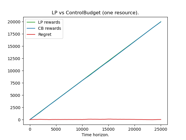
(a) ControlBudget with one resource - case 1 (positive drift arm)

(b) ControlBudget with one resource - case 2 (null plus negative drift arm)

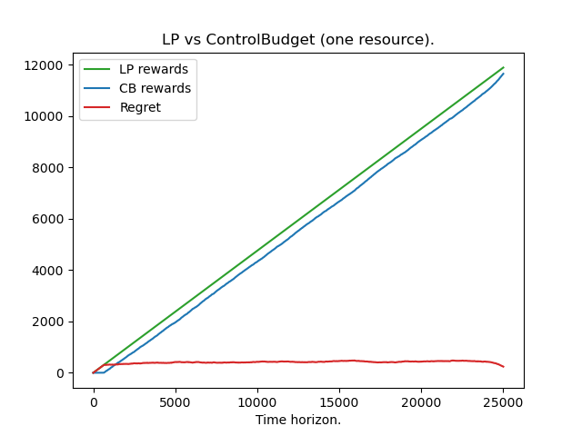
(c) ControlBudget with one resource - case 3 (positive plus negative drift arm)

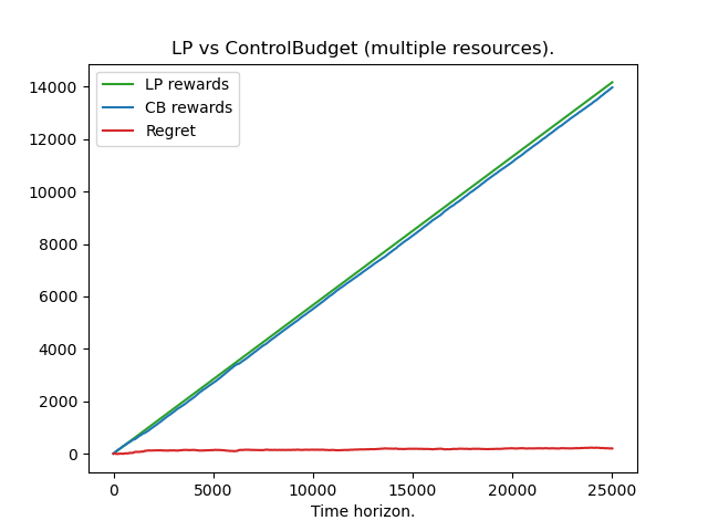
(d) ControlBudget with multiple resources

Figure 1: Regret of ControlBudget on a variety of test cases.

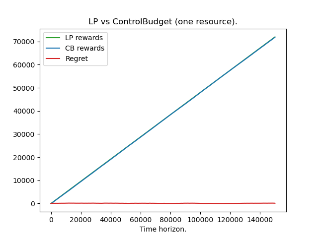
(a) ControlBudget

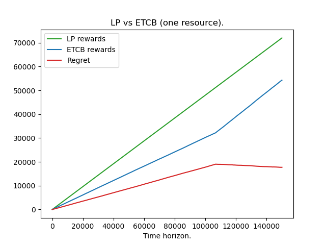
(b) ExploreThenControlBudget

Figure 2: Regret of ControlBudget and ExploreThenControlBudget on the same test case. We modify ExploreThenControlBudget to use the empirical means instead of UCB/LCB estimates for phase one as described in  Appendix F.

As our plots show (Fig. 1), our MDP policy, ControlBudget, performs quite well and achieves constant regret.

Our learning algorithm does not perform as well empirically due to large constant factors. Specifically, the number of rounds required for the confidence radius to be small enough for phase one to successfully identify $X^{*}$ and $J^{*}$ is too large. In our simple test cases, if we simply consider the empirical means, which are very close to the true means, instead of the UCB/LCB estimates for phase one, then the learning algorithm performs as expected: it achieves logarithmic regret by spending a logarithmic number of rounds identifying $X^{*}$ and $J^{*}$, and achieves constant regret thereafter (Fig. 2).

References

• Agrawal and Devanur [2016] Shipra Agrawal and Nikhil Devanur. Linear contextual bandits with knapsacks. Advances in Neural Information Processing Systems, 29, 2016.
• Agrawal and Devanur [2014] Shipra Agrawal and Nikhil R Devanur. Bandits with concave rewards and convex knapsacks. In Proceedings of the fifteenth ACM conference on Economics and computation, pages 989–1006, 2014.
• Auer et al. [2002a] Peter Auer, Nicolo Cesa-Bianchi, and Paul Fischer. Finite-time analysis of the multiarmed bandit problem. Machine learning, 47(2):235–256, 2002a.
• Auer et al. [2002b] Peter Auer, Nicolo Cesa-Bianchi, Yoav Freund, and Robert E Schapire. The nonstochastic multiarmed bandit problem. SIAM journal on computing, 32(1):48–77, 2002b.
• Badanidiyuru et al. [2013] Ashwinkumar Badanidiyuru, Robert Kleinberg, and Aleksandrs Slivkins. Bandits with knapsacks. In 2013 IEEE 54th Annual Symposium on Foundations of Computer Science, pages 207–216. IEEE, 2013.
• Badanidiyuru et al. [2018] Ashwinkumar Badanidiyuru, Robert Kleinberg, and Aleksandrs Slivkins. Bandits with knapsacks. Journal of the ACM (JACM), 65(3):1–55, 2018.
• Bubeck and Cesa-Bianchi [2012] Sébastien Bubeck and Nicolò Cesa-Bianchi. Regret analysis of stochastic and nonstochastic multi-armed bandit problems. Found. Trends Mach. Learn., 5(1):1–122, 2012.
• Even-Dar et al. [2002] Eyal Even-Dar, Shie Mannor, and Yishay Mansour. Pac bounds for multi-armed bandit and markov decision processes. In International Conference on Computational Learning Theory, pages 255–270. Springer, 2002.
• Flajolet and Jaillet [2015] Arthur Flajolet and Patrick Jaillet. Logarithmic regret bounds for bandits with knapsacks. arXiv preprint arXiv:1510.01800v4, 2015.
• Immorlica et al. [2019] Nicole Immorlica, Karthik Abinav Sankararaman, Robert Schapire, and Aleksandrs Slivkins. Adversarial bandits with knapsacks. In 2019 IEEE 60th Annual Symposium on Foundations of Computer Science (FOCS), pages 202–219. IEEE, 2019.
• Kleinberg et al. [2019] Robert Kleinberg, Aleksandrs Slivkins, and Eli Upfal. Bandits and experts in metric spaces. Journal of the ACM (JACM), 66(4):1–77, 2019.
• Lai et al. [1985] Tze Leung Lai, Herbert Robbins, et al. Asymptotically efficient adaptive allocation rules. Advances in applied mathematics, 6(1):4–22, 1985.
• Lattimore and Szepesvári [2020] Tor Lattimore and Csaba Szepesvári. Bandit algorithms. Cambridge University Press, 2020.
• Li et al. [2021] Xiaocheng Li, Chunlin Sun, and Yinyu Ye. The symmetry between arms and knapsacks: A primal-dual approach for bandits with knapsacks. In International Conference on Machine Learning, pages 6483–6492. PMLR, 2021.
• Sankararaman and Slivkins [2021] Karthik Abinav Sankararaman and Aleksandrs Slivkins. Bandits with knapsacks beyond the worst case. Advances in Neural Information Processing Systems, 34, 2021.
• Slivkins [2011] Aleksandrs Slivkins. Contextual bandits with similarity information. In Proceedings of the 24th annual Conference On Learning Theory, pages 679–702. JMLR Workshop and Conference Proceedings, 2011.
• Slivkins [2019] Aleksandrs Slivkins. Introduction to multi-armed bandits. Found. Trends Mach. Learn., 12(1-2):1–286, 2019.
• Tran-Thanh et al. [2010] Long Tran-Thanh, Archie Chapman, Enrique Munoz De Cote, Alex Rogers, and Nicholas R Jennings. Epsilon–first policies for budget–limited multi-armed bandits. In Twenty-Fourth AAAI Conference on Artificial Intelligence, 2010.
• Tran-Thanh et al. [2012] Long Tran-Thanh, Archie Chapman, Alex Rogers, and Nicholas Jennings. Knapsack based optimal policies for budget–limited multi–armed bandits. In Proceedings of the AAAI Conference on Artificial Intelligence, volume 26, pages 1134–1140, 2012.