Notes on Hydraulic Fracture Mechanics

Abstract

These notes address mechanics of propagating hydraulic fractures (HF). In the first part, we focus on how different physical mechanisms (dissipation in fluid and solid, fluid storage in fracture and its exchange with permeable rock, crack elasticity) manifest near the fracture tip and lead to a ‘zoo’ of fracture propagation regimes, as correspond to different coupling of predominant mechanisms depending on material parameters and fracture propagation speed. In the second part, we illustrate how different near-tip regimes dictate the propagation of finite fractures of simple geometries (e.g. 2D plane-strain, or 3D radial cracks) driven by fluid injection at the center of the crack. These notes are not a review of the research on the topic, which has seen tremendous renewed interest in the last 20 years or so, (for a review see, e.g., [1]); but rather an attempt to introduce the mechanics and physics of HF in a simple and hopefully-logical way, from the fracture tip to a finite fracture propagation.

Dalhousie University, Department of Civil and Resource Engineering, Halifax, Canada

1 Boundary Layer Structure Near Tip of Propagating Hydraulic Fracture via Williams-like expansions

Here we will explore how the presence of fluid at the propagating fracture tip may impact the near tip fracture behavior in the context of limiting propagation regimes dominated by a subset of the physical processes. These processes can be simply identified with two energy dissipation mechanisms in the HF:

• dissipation in generation of new fracture surface, i.e. the classical fracture energy or toughness, and

• the viscous dissipation in the fluid flow within the fracture

and with two fluid storage mechanisms

• in the fracture, and

• in the surrounding permeable rock (leak-off).

1.1 William’s solution of elasticity

Recall Williams’ power-law solution for a semi-infinite Mode I (symmetric) plane-strain crack in infinite elastic domain

Figure 1: Semi-infinite crack and related definitions.

for the Airy Stress Function [2, 3]

$$\phi=r^{\lambda+1}(A_{1}\cos(\lambda+1)\theta+A_{2}\sin(\lambda-1)\theta)$$

(a power law form which satisfies the biharmonic equation $\nabla^{4}\phi=0$), stress

$$\sigma_{r\theta} =r^{\lambda-1}\left(A_{1}\lambda(\lambda+1)\sin(\lambda+1)\theta+A_{2}\lambda(\lambda-1)\sin(\lambda-1)\theta\right)$$ (1)

$$\sigma_{\theta\theta} =r^{\lambda-1}\left(A_{1}\lambda(\lambda+1)\cos(\lambda+1)\theta+A_{2}\lambda(\lambda-1)\cos(\lambda-1)\theta\right)$$

and displacements

$$u_{r} =\frac{1}{2\mu}r^{\lambda}\left(-A_{1}(\lambda+1)\cos(\lambda+1)\theta+A_{2}(\kappa-\lambda)\cos(\lambda-1)\theta\right)$$ (2)

$$u_{\theta} =\frac{1}{2\mu}r^{\lambda}\left(A_{1}(\lambda+1)\sin(\lambda+1)\theta+A_{2}(\kappa+\lambda)\sin(\lambda-1)\theta\right)$$

where $\kappa=3-4\nu$ (plane strain) and $\mu$ is the shear modulus. (In plane strain problems, we will make use of the so-called plane-strain elastic modulus, $E^{\prime}=2\mu/(1-\nu)$).

This solution can be used to construct a variety of hydraulic fracture tip solutions characterized by power-law tractions along the fracture faces. Coefficients $A_{1}$ and $A_{2}$ are recovered as part of the solution of a particular problem in the following.

1.2 Fluid flow in a steadily propagating fracture in impermeable rock

1.2.1 Impermeable solid

Consider hydraulic fracture tip propagating at a steady velocity $V$ on assumption that the fluid flow in the fracture is able to “keep up” with the fracture tip. Conservation of mass (volume for an incompressible fluid) suggests that fluid flow velocity is

$$v_{f}=V$$ (3)

where the fluid velocity is given by the Poiseuille’s law for pressure-gradient driven flow

$$v_{f}=\frac{w^{2}}{\eta^{\prime}}\frac{dp_{f}}{dr}$$ (4)

in a channel of aperture

$$w=u_{\theta}(-\pi)-u_{\theta}(+\pi),$$

(Here $\eta^{\prime}=12\eta_{f}$ is a fluid viscosity parameter and $p_{f}$ is the fluid pressure.)

1.2.2 Permeable solid (fluid leak-off)

A fracture pressurized by a fluid at $p_{f}\sim\sigma_{o}$ would necessarily leak fluid off to the surrounding rock, if a) the rock is sufficiently permeable and b) the ambient pore fluid pressure in the rock $p_{o}$ is less than the fracturing fluid pressure, i.e. $p_{o}<p_{f}$. The latter condition is typically satisfied since the ambient pore pressure is (much) smaller than the ambient stress, $p_{o}<\sigma_{o}$.

On assumption $p_{o}\ll\sigma_{o}\sim p_{f}$, the leak-off can be modeled as from approximately constant fluid pressure step (from $p_{o}$ to $p_{f}\sim\sigma_{o}$) from the moment of the arrival $t\geq t_{o}(x)$ of the fracture tip at a given position $x$ along the fracture path. Limiting the diffusion considerations to the 1D (the leak-off boundary layer around the fracture is small compared to a pertinent fracture lengthscale, e.g. length for finite fractures), the rate of leak-off is then $g(x)=C^{\prime}/\sqrt{t-t_{o}(x)}$ where $C^{\prime}$ is so-called Carter’s leak-off coefficient incapsulating the rock parameters and proportional to the imposed fluid pressure step at the fracture wall $\approx\sigma_{o}-p_{o}$).

The fracturing fluid balance equation

$$\frac{\partial w}{\partial t}+\frac{\partial wv_{f}}{\partial x}+g=0$$

when rewritten in the frame moving with crack tip, $r=Vt-x$ and $\theta=\pm\pi$, becomes

$$V\frac{dw}{dr}-\frac{dwv_{f}}{dr}+g=0$$

where the leak-off rate can be now expressed as $g=C^{\prime}\sqrt{V}/\sqrt{r}$ (since the crack arrival time at fixed position $x=Vt-r$ can be expressed as $t_{o}(x)=r/V$). Integrating the above equation from the tip $r=0$ to some $r>0$ and using tip closure condition $w_{|r=0}=wv_{|r=0}=0$, we finally recover

$$wv_{f}=wV+2C^{\prime}\sqrt{Vr}$$ (5)

Compare this to the impermeable case fluid balance, $v_{f}=V$, to appreciate that the fluid inflow into the tip region bounded by some $r$ (i.e. $wv_{f}$) is partitioned between the fluid stored in that crack tip region (i.e. $wV$) and the fluid leaked-off into the rock from that region (i.e. $\int_{0}^{r}gdr=2C^{\prime}\sqrt{Vr}$). Thus, the right hand side of this equation simply presents the fluid partition between crack storage and “rock storage” (or leak-off).

(a)

(b)

Figure 2: Linear decomposition of the HF problem when distribution of normal traction on the crack walls (fluid pressure) is (a) uniform and (b) non-uniform.

1.3 Uniformly loaded HF - Toughness-dominated solution
(negligible viscous pressure drop in the crack)

In the limiting case when the fluid pressure drop in the flow towards the fracture tip is negligible (e.g., when fluid viscosity $\eta^{\prime}$ is negligible), i.e. $p_{f}$ is approximately uniform along the crack, the problem can be decomposed into that of (i) a zero-traction crack in the elastic domain loaded by tensile far field stress which value is given by the fluid net pressure, $\sigma_{yy}(x,y\rightarrow\infty)=p=p_{f}-\sigma_{o}$; and (ii) the uniformly stressed elastic domain (without the crack), $\sigma_{yy}(x,y)=-p_{f}$ (see Figure 2a).

Zooming into the crack tip region of the crack in sub-problem (i), we recover a semi-infinite, traction-free crack (Figure 1) with

$$\sigma_{\theta\theta}(\theta=\pm\pi)=0\qquad\sigma_{r\theta}(\theta=\pm\pi)=0$$

This is of course a familiar (by now) problem of the zero-traction crack tip field, which solution follows from evaluating the above boundary conditions using the Williams’ solution (1). This is an eigenvalue problem, which solution leads to the LEFM power-law $\lambda=1/2$ and a relation between the two unknown coefficients $A_{1}$ and $A_{2}$ in (1). Eliminating $A_{2}$ and redefining the unknown $A_{1}\Rightarrow K_{I}/(3\sqrt{2\pi})$, we get the crack tip solution for the zero-traction semi-infinite crack in the form

$$\left(\begin{array}[]{c}\sigma_{r\theta}\\ \sigma_{\theta\theta}\end{array}\right)=\frac{K_{I}}{\sqrt{2\pi r}}\left(\begin{array}[]{c}\sin\theta\,\cos^{2}\frac{\theta}{2}\\ \cos^{3}\frac{\theta}{2}\end{array}\right)\qquad\left(\begin{array}[]{c}u_{r}\\ u_{\theta}\end{array}\right)=\frac{4K_{I}}{E^{\prime}(1-\nu)}\sqrt{\frac{r}{2\pi}}\left(\begin{array}[]{c}\cos\frac{\theta}{2}\,\left(1-\frac{1+\cos\theta}{4(1-\nu)}\right)\\ -\sin\frac{\theta}{2}\,\left(1-\frac{1+\cos\theta}{4(1-\nu)}\right)\end{array}\right)$$

$K_{I}$ with units [Pa$\sqrt{\text{m}}$] is the so-called mode I stress intensity factor (SIF), as it gives the “strength” of the $1/\sqrt{r}$ stress singularity of the stress ahead of the tip. More specifically, the tensile singular stress ahead of the fracture tip, acting to “open”/advance the crack along its plane ($\theta=0$) is varying with distance $r$ ahead of the tip as

$$\sigma_{yy}(r,\theta=0)=\frac{K_{I}}{\sqrt{2\pi r}}$$

while the crack opening is varying with distance $r$ behind the crack tip as

$$w(r)=u_{\theta}(r,-\pi)-u_{\theta}(r,+\pi)=\frac{8K_{I}}{E^{\prime}}\sqrt{\frac{r}{2\pi}}$$ (6)

When zooming to the traction-free fracture tip in the subproblem (i) of Figure 2a, we essentially “lost” the information about the global (far-field) tensile loading, which keeps the finite fracture open/advancing, and, thus, determines the magnitude of the stress intensity factor. In other words $K_{I}$ is inherently global loading characteristic, which provides a link between the finite fracture and its (far field in our case) loading and the its near tip behavior.

We will be able to evaluate $K_{I}$ for a given global fracture problem of interest, once the elasticity equation for a crack of a finite geometry is formulated. Notwithstanding, for propagating fractures, the value of $K_{I}$ is constrained by the propagation criterion, which matches the potential elastic energy ($d\varPi$) that can be released into the crack tip region upon advancing the crack a unit distance (a unit surface area, $d\Sigma$) to the fracture energy $G_{c}$, a material property corresponding to the energy dissipation involved in creating a unit of (two) new surfaces. The former, referred to as the energy release rate $G$, is actually uniquely defined by the elastic crack field [4]

$$G=-\frac{d\varPi}{d\Sigma}=\lim_{\Delta\ell\rightarrow 0}\frac{1}{2\Delta\ell}\int_{0}^{\Delta\ell}\sigma_{yy}^{(0)}(r,\theta=0)\,w^{(\Delta\ell)}(\Delta\ell-r)\,dr$$ (7)

where the “$(0)$” and “$(\Delta\ell)$” refer to the fields before and after crack tip advance by $\Delta\ell$. Evaluating, leads to a simple relation of the energy release rate to the stress intensity factor at the crack tip

$$G=\frac{K_{I}^{2}}{E^{\prime}}$$

(The result, which up to a numerical prefactor, follows from units considerations, where the energy release rate G [J/m²=Pa m] is ought to be expressed in terms the only two dimensional parameters defining the LEFM crack tip fields, i.e. $K_{I}$ [Pa$\sqrt{\text{m }}$] and elastic modulus $E^{\prime}$ [Pa]).

The propagation criterion $G=G_{c}$, can be reformulated in terms of the critical value of the stress intensity factor (referred to as material “toughness”) $K_{Ic}=\sqrt{G_{c}E^{\prime}}$, as

$$K_{I}=K_{Ic}$$ (8)

and corresponding tip stress/displacement fields uniquely defined for propagating fracture.

Defining the lenghthscale

$$\ell_{k}=\left(\frac{K^{\prime}}{E^{\prime}}\right)^{2}$$

where for brevity

$$K^{\prime}=\sqrt{\frac{32}{\pi}}K_{Ic}$$

the opening distribution (6) with (8) for the toughness-dominated propagating fracture can be rewritten as

$$w=\ell_{k}^{1/2}r^{1/2}$$ (9)

1.4 Non-uniformly loaded HF (negligible fracture toughness)

1.4.1 Impermeable solid

Consider now the case where viscous dissipation in the fluid flow is important, and suggest that the net fluid pressure $p(r)=p_{f}(r)-\sigma_{o}$ in the subproblem (i) of Figure2b (i.e. hydraulic fracture driven by $p$ in otherwise relaxed solid) is some power-law of the distance $r$ from the tip, in the crack tip vicinity (modeled as a semi-infinite crack),

$$p(r)=-B\,r^{\lambda-1}$$ (10)

where prefactor $B$ and power law exponent $\lambda$ are unknowns.

Corresponding traction boundary conditions on the semi-infinite crack walls are

$$\theta=\pm\pi:\qquad\sigma_{r\theta}=0\qquad\sigma_{\theta\theta}=-p(r)=B\,r^{\lambda-1}$$

Corresponding Williams’ solution coefficients satisfying the above boundary conditions are

$$A_{1}=-B\frac{\lambda-1}{\lambda+1}\frac{1}{2\lambda\cos\pi\lambda}\qquad A_{2}=-B\frac{1}{2\lambda\cos\pi\lambda}$$

and the crack opening

$$w(r)=u_{\theta}(r,-\pi)-u_{\theta}(r,+\pi)=\frac{B}{E^{\prime}}\varphi(\lambda)\,r^{\lambda}$$ (11)

where $\varphi(\lambda)=4\lambda^{-1}\tan(1-\lambda)\pi$.

Plugging the above power laws for the net pressure and opening into the fluid lubrication equation for impermeable solid, $v_{f}=V$, with $v_{f}=(w^{2}/\eta^{\prime})(dp_{f}/dr)$ and $dp_{f}=dp$ (uniform far field confining stress $d\sigma_{o}/dr=0$), we recover the power law $\lambda=2/3$ and the prefactor $B=\delta_{m}(V\eta^{\prime}E^{\prime 2})^{1/3}$ with $\delta_{m}=6^{-2/3}$.

Defining lengthscale

$$\ell_{m}=\frac{V\eta^{\prime}}{E^{\prime}}$$

final expressions for the near HF tip viscous-dominated solution [5]

$$\sigma_{yy}(\theta=\pm\pi)=-p=\delta_{m}\,E^{\prime}\,(\ell_{m}/r)^{1/3}\qquad w=\delta_{m}\varphi(2/3)\,\ell_{m}^{1/3}r^{2/3}$$ (12)

This solution suggests that the viscosity-dominated propagating crack tip is sharper/narrower than the toughness dominated one ($r^{1/2}\gg r^{2/3}$ when $r\rightarrow 0$) and that the fluid undergoes suction ($p$ and $p_{f}$ are negative close to the tip) diverging towards the fracture tip.

For the stress ahead of the fracture tip we can recover from the solution $\sigma_{yy}(\theta=0)=2B/r^{1/3}$, which suggests a tensile singularity at the tip approached from the intact solid, but a weaker one than the LEFM one ($\sim 1/r^{1/2}$). This state of affairs naturally implies that the energy release rate (7) at the viscosity-dominated crack tip is zero, $G=0$, and that in view of the fracture propagation criterion $G=G_{c}$, the explored solution is strictly valid only in the zero-toughness limit. As we will observe in the following, this seeming contradiction can be reconciled, and the two limiting (toughness- and viscosity-dominated) solution arise as the near (small $r$) and far (large $r$) fields of the more general HF tip solution to be discussed in the following.

1.4.2 Permeable solid (leak-off)

Consider now the case of non-negligible fluid leak-off into the permeable solid around it. To appreciate the importance of the leak-off to the fracture propagation, assume for a moment that the leak-off effect is small and use the zero-leak-off viscosity-dominated solution derived in the above to evaluate the terms in the right hand side of the fluid balance equation (5), i.e. the partition between the crack fluid storage $wV$ and the leak-off $\int_{0}^{r}gdr=2C^{\prime}\sqrt{Vr}$. The former is $\propto r^{2/3}$ while the latter $\propto r^{1/2}$, suggesting that the fluid balance in the crack will be dominated by the crack-storage at large distances from the tip while the leak-off (i.e. fluid storage in the rock) will dominate at small distances from the tip.

The near-field, leak-off dominated solution can be recovered by the same solution procedure as in the impermeable case above, when applied to the leak-off dominated fluid balance equation end-member $wv_{f}=2C^{\prime}\sqrt{Vr}$ (i.e. when neglecting the storage term $wV$ in the right hand side) with $v_{f}=(w^{2}/\eta^{\prime})(dp/dr)$. Plugging the power law forms for the net pressure (10) and crack opening (11) into the fluid balance end-member, we recover the power law $\lambda=5/8$ and the prefactor $B=\delta_{\widetilde{m}}\,\left(C^{\prime}\sqrt{V}\eta^{\prime}E^{\prime 3}\right)^{1/4}$ with $\delta_{\widetilde{m}}=\left(\frac{125}{6144}\tan^{3}\frac{\pi}{8}\right)^{1/4}$.

Defining lengthscale

$$\ell_{\widetilde{m}}=\left(\frac{C^{\prime}\sqrt{V}\eta^{\prime}}{E^{\prime}}\right)^{2/3}$$

we can write the final expressions for the near HF tip viscous-dominated solution under conditions of dominant leak-off [6]

$$\sigma_{yy}(\theta=\pm\pi)=-p=\delta_{\widetilde{m}}\,E^{\prime}\,(\ell_{\widetilde{m}}/r)^{3/8}\qquad w=\delta_{\widetilde{m}}\varphi(5/8)\,\ell_{\widetilde{m}}^{3/8}r^{5/8}$$ (13)

Similarly to the solution for the viscosity-dominated crack tip in the impermeable solid, the leak-off (permeable solid) dominated solution corresponds to the zero energy release rate, and thus strictly realized in the zero-toughness

1.5 General HF tip solution [7, 8]

In the above, we have recovered three limiting solutions for the problem of semi-infinite hydraulic fracture propagation, recounted below for their fracture opening distributions:

• the toughness-dominated ($k$) solution ($\eta^{\prime}=0$), $w=\ell_{k}^{1/2}r^{1/2}$

• the viscosity-storage-dominated ($m$) solution ($K^{\prime}=0$, $C^{\prime}=0$), $w\sim\ell_{m}^{1/3}r^{2/3}$

• the viscosity-leak-off-dominated ($\widetilde{m}$) solution ($K^{\prime}=0$, $C^{\prime}\rightarrow\infty$), $w\sim\ell_{\widetilde{m}}^{3/8}r^{5/8}$

with their respective lengthscales $\ell_{k}$, $\ell_{m}$, and $\ell_{\widetilde{m}}$.

The structure of the general solution (i.e. for arbitrary set of values of fluid viscosity $\eta^{\prime}$, solid toughness$K_{Ic}$, and fluid leak-off $C^{\prime}$ parameters), is hinted by the order of the corresponding power law exponents in the limiting expressions for the crack opening

$$1/2<5/8<2/3$$

which suggests that if all three (or any two of the three) limiting regimes are to be realized in the general hydraulic fracture solution, they would appear/dominate at different spatial scales (distances from the tip): the $k$-solution in the near field ($r\rightarrow 0$), the $m$-solution in the far field ($r\rightarrow\infty$), and the $\widetilde{m}$-solution possibly in the intermediate field (i.e. at intermediate distances from the tip)

$$k\rightarrow(\widetilde{m})\rightarrow m$$ (14)

( arrows indicate the transition with distance away from the fracture tip). This solution structure can be visualized in a triangular parametric diagram $m\widetilde{m}k$ [8], where the vertices correspond to the three limiting solutions, and a trajectory reflect a progression of the solution with the increasing distance from the tip, always starting from $k$-vertex and ending in the $m$-vertex (Figure 3).

Figure 3: Semi-infinite HF parametric space (a), and the structure of the small ($\chi\ll 1$) and large $(\chi\gg 1$) leak-off solutions, after [8].

The edges of this parametric space correspond to the propagation regimes dominated by either one dissipation mechanism or one fluid-storage mechanism. For example, the storage $mk$-edge corresponds to the case of negligible leak-off (impermeable solid, $C^{\prime}=0$), which solution is expected to transition from the toughness-dominated $k$-vertex in the near field to the storage-viscosity dominated $m$-vertex in the far field. The characteristic lengthscale $\ell_{mk}$ of this transition can be estimated by evaluating the distance from the tip where the $k$ and $m$ asymptotes “intersect”, i.e. $\ell_{k}^{1/2}r^{1/2}\sim\ell_{m}^{1/3}r^{2/3}$ at $r\sim\ell_{mk}$, which gives

$$\ell_{mk}=\frac{\ell_{k}^{3}}{\ell_{m}^{2}}=\frac{K^{\prime 6}}{E^{\prime 4}V^{2}\eta^{\prime 2}}$$

Exploring the other two edges in the similar fashion we get that the viscosity $m\widetilde{m}$-edge corresponds to negligible solid toughness ($K_{Ic}=0$), and its expected solution transitions from the viscosity-leak-off dominated $\widetilde{m}$-vertex in the near field to the viscosity-storage dominated $m$-vertex in the far field. The corresponding transition lengthscale

$$\ell_{m\widetilde{m}}=\frac{\ell_{\widetilde{m}}^{9}}{\ell_{m}^{8}}=\frac{C^{\prime 6}E^{\prime 2}}{V^{5}\eta^{\prime 2}}$$

Finally, the $\widetilde{m}k$-edge corresponds to the case with negligible storage ($C^{\prime}\rightarrow\infty$), and its expected solution transitions from the toughness-dominated $k$-vertex to the viscosity-leak-off-dominated $\widetilde{m}$-vertex with the distance from the tip, with the characteristic transition lengthscale

$$\ell_{\widetilde{m}k}=\frac{\text{$\ell_{k}^{4}$}}{\ell_{\widetilde{m}}^{3}}=\frac{K^{\prime 8}}{E^{\prime 6}C^{\prime 2}V\eta^{\prime 2}}$$

It can then be foreseen that for “small” leak-off, the solution is closely approximated by the $mk$-edge

$$k\underset{\ell_{mk}}{\rightarrow}m\quad(\text{"small" }C^{\prime})$$

As the leak-off parameter is increased, the solution trajectory is dragged towards the leak-off-viscosity $\widetilde{m}$-vertex (while the near and far fields are invariantly at the $k$ and $m$ vertices, respectively), such that in the limit of “large” leak-off the solution structure with complete set of the near ($k$), intermediate $(\widetilde{m}$), and far ($m$) field asymptotes is realized

$$k\underset{\ell_{\widetilde{m}k}}{\rightarrow}\widetilde{m}\underset{\ell_{m\widetilde{m}}}{\rightarrow}m\quad(\text{"large" }C^{\prime})$$

It is now clear that in the latter “large” leak-off case, the two corresponding transition lengthscales have to separate, i.e.

$$\ell_{\widetilde{m}k}\ll\ell_{m\widetilde{m}}\quad(\text{"large" }C^{\prime})$$

which then suggests a single non-dimensional parameter, $\ell_{m\widetilde{m}}/\ell_{\widetilde{m}k}$, to quantify the “smallness” or “largeness” of leak-off, and, thus, fully parametrize a solution trajectory in the parametric space. More specifically, we can define non-dimensional leak-off parameter

$$\chi=\left(\frac{\ell_{m\widetilde{m}}}{\ell_{\widetilde{m}k}}\right)^{1/8}=\frac{C^{\prime}E^{\prime}}{V^{1/2}K^{\prime}}$$

to parametrize the general HF tip solution (Figure 3).

1.5.1 Towards complete HF tip formulation and obtaining the complete tip solution

In order to solve the general HF tip problem, which anticipated spatial fracture and parametric dependence has been addressed above, we need to appeal to more general description of the crack elasticity than the Williams’ power law class of solutions utilized in so far. That general elastic framework can be furnished in the form the crack boundary integral equation, which models the distribution of crack opening as a “pile-up” of dislocations, as discussed in the preceding chapters.

To briefly recount, we use the solution for a unit gap opened along semi-infinite line $y=0$, $x>0$ (or $\theta=0$ in polar coordinates), $u_{\theta}(\theta=0^{+})-u_{\theta}(\theta=0^{-})=1$, (so called “climb” dislocation) for the distribution of stress normal to the dislocation plane $\sigma_{yy}^{D}(x,y=0)=-E^{\prime}/4\pi x$. Noting that arbitrary distribution of opening $w(x)$ can be obtained as pile-up of infinitesimal climb-dislocations $dw(s)$ positioned along the crack $s\in crack$, the corresponding stress distribution along the crack plane is obtained by superposition

Figure 4: Crack as a pile-up of infinitesimal dislocations.

$$\sigma_{yy}(x,y=0)=\int_{crack}\sigma_{yy}^{D}(x-s,y=0)\,\frac{dw}{ds}ds$$ (15)

In the particular case of a semi-infinite crack, in the coordinate frame moving with the crack tip, $r=x_{tip}(t)-x$ for $\theta=\pm\pi$, the above elasticity equation takes the following form along the crack

$$\sigma_{yy}(r,\theta=\pm\pi)=-p(r)=-\frac{E^{\prime}}{4\pi}\int_{0}^{\infty}\frac{dw}{ds}\frac{ds}{r-s}$$ (16)

(this stress expression applies ahead of the crack tip, $\theta=0$, upon substitution $r\Rightarrow-r$).

General solution for the HF tip is then obtained by solving simultaneously, the crack elasticity (16), fluid continuity (5) with the Poiseuille law (4), and the propagation condition (9) at $r\rightarrow 0$. The numerical solution can be furnished by a variety of methods, including the method described in [GaDe11] and, more recently, a method based on Gauss-Chebyshev calculus for classical (dry) crack problems [9] applied to HF [10].

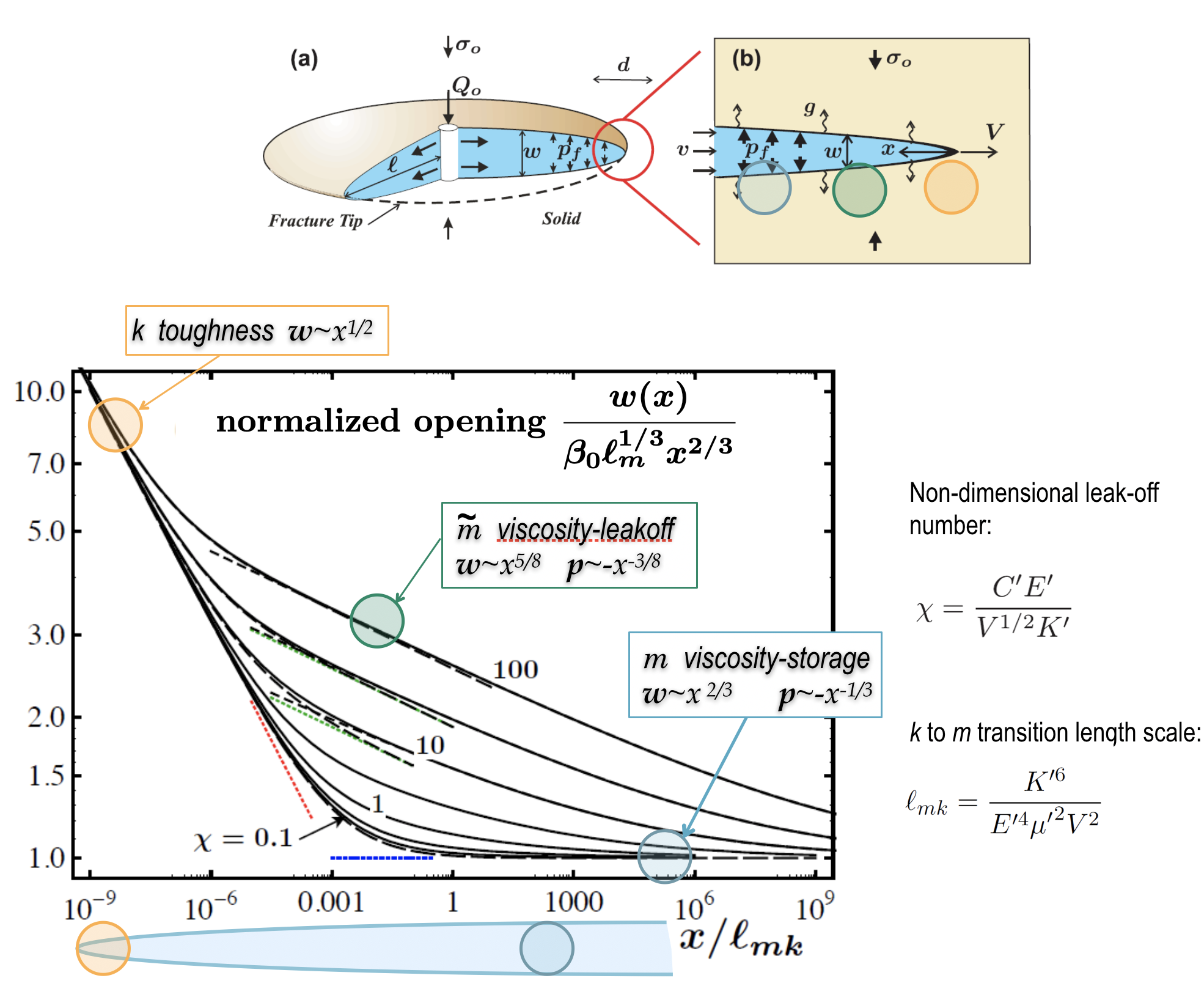
Figure 5: Semi-infinite HF general solution for the opening normalized by the far-field ($m$) asymptote for different values of the non-dimensional leak-off parameter $\chi$, adopted from [8].

1.6 Some physical constraints/limitations on Hydraulic Fracture Tip Model

The physical limitations of the presented HF tip model are sketched here, as they emerge from the considerations for the solid and fluid, respectively. This delineation is somewhat superficial, as the coupling between the fluid flow and solid rupture is the $O(1)$ effect that would modify the physical manifestation of the processes.

1.6.1 Solid

• LEFM stress singularity $\Rightarrow$ emergence of a finite non-elastic region at/ahead the crack tip where the solid undergoes degradation/decohesion. This fracture “process zone” is often modeled as the extension of the crack along its plane (i.e. material degradation zone is “collapsed” for the sake of modeling onto the fracture plane) along which the cohesive tractions between the nascent fracture surfaces evolve from the peak material cohesion (at zero fracture opening) to zero cohesion (at certain critical crack surface separation/opening $w_{c}$).

• Apparent fracture energy (energy to be spent in creation of a unit of the nominal fracture surface, i.e. projection of the real/rough surfaces onto the mean plane) is likely not a fixed material property, but rather scales with the fracture growth

1.6.2 Fluid

• Singular fluid suction at the tip of fully-fluid-filled propagating crack $\Rightarrow$ emergence of a finite fluid lag - a near tip region filled by fracturing fluid vapor/volatiles (in the case of impermeable rock) or/and by the pore fluid sucked into the lag from the surrounding permeable rock [11]

• Coupling of the fluid (lag) and the solid (decohesion) process zones via the fluid flow [12]

• Fracture surface rough topography about nominally-flat fracture plane may lead to the enhanced dissipation in the viscous fluid flow (departure from the Pouiseille flow between two parallel, flat plates)

• Fluid viscous drag on the fracture surfaces in the direction of the flow (i.e. towards the fracture tip) [13]

2 Finite HF of Simple Geometries (homogeneous rock and in-situ stress field)

Under conditions of homogeneous (spatially uniform), isotropic rock properties and homogeneous in-situ stress field, hydraulic fractures would tend to propagate along a single plane normal to the direction of the minimum (compressive) in-situ stress, referred to as the fracture confining stress $\sigma_{o}$. Aside from shallow depth cases, the minimum in-situ stress is usually horizontal, leading to a vertical hydraulic fracture plane.

The expected fracture geometry within its plane is defined by the dimensionality of the fluid source. In the following, we adopt a fixed coordinate system $x$ (fracture propagation direction), $y$ (fracture opening direction), and $z$ (fracture height direction.

• A circular (penny-shape) fracture geometry as the result of radial propagation from a point fluid source, approximating a localized perforated interval of a otherwise cased wellbore. The wellbore orientation (vertical, horizontal, or inclined) does not reflect on the fracture geometry in this fluid source idealization. In this case the fracture dimensions are: the instantaneous fracture radius $\ell(t)$ (distance from the fluid source to the current location of the circular fracture front, $r=\ell(t)$ in the vertical x-z fracture plane, in the coordinate system with the origin at the fluid source) and the opening $w(r,t)$ with $0<r<R(t)$

• A plane-strain, bi-wing fracture geometry as the result of propagation from a line fluid source, approximating a spatially extended perforated interval of a vertical wellbore (Figure 6). This fracture geometry is referred to as KGD-fracture (after Khristianovic, Zheltov, Geertsma and De Klerk [14, 15]). The fracture dimensions are: the instantaneous half-length of the fracture $\ell(t)$ in the (bi-)propagation direction(s) away from the line fluid source and the opening $w(x,t)$, $-\ell(t)<x<\ell(t)$, with $x=y=0$ giving the location of the line source. The plane-strain approximation is the result of taking the third fracture dimension -its height - as infinite (similarly approximating the line fluid source as infinite), such that any horizontal cross-section (x-y planes) of the fracture is identical to another.

• A third simplified hydraulic fracture geometry commonly considered is the so-called PKN (after Perkins, Kern and Nordgren [16, 17]), or fracture with constrained height, which postulates a bi-wing fracture with a fixed height $h=const$ and half-length $\ell(t)\gg h$. Physically, the fixed height approximation emerges from the lithological/stress vertical heterogeneity - where the more competent cap-rock layers, above and below the hydraulically-stimulated (reservoir) layer of height $h$, support higher level of confining stress, effectively suppressing the hydraulic fracture height growth into the cap-rock. The main modeling approximation emerging from the elongated fracture geometry ($\ell\gg h$) is the plane-strain approximation for any vertical cross-section (y-z planes) of the fracture.

The above simplified fracture geometry reduce the problem dimensionality to 1D (in the direction of fracture propagation), allowing for a variety of (semi) analytical approaches, providing basic understanding of propagation of finite volume hydraulic fractures and their parametric regimes, and also serve as benchmarks for numerical methods been developed for more general treatment of the hydraulic fracture problem (e.g., the 2 or 3D geometries, non-uniform and anisotropic properties and stress, near wellbore effects, etc, see [18] for a recent review).

2.1 KGD Fracture Formulation

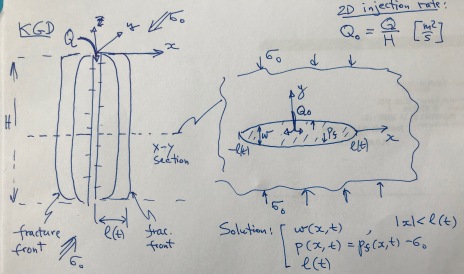
Figure 6: KGD fracture model: (left) bi-wing vertical hydraulic fracture of half-length $\ell(t)$ propagating from the line source with fluid injection rate $Q$ distributed over height $H\gg\ell$; (tight) horizontal 2D cross-section corresponding to a plane-strain crack driven by 2D injection rate $Q_{o}=Q/H$.

Field (crack line) equations:

• Crack elasticity (dislocation pile-up)

  $$\sigma_{yy}(x,y=0,t)=-p(x,t)=-\frac{E^{\prime}}{4\pi}\int_{-\ell(t)}^{+\ell(t)}\frac{\partial w(s,t)}{\partial s}\frac{ds}{x-s}$$ (17)

• Fluid flow (continuity and Poiseuille’s law)

  $$\frac{\partial w}{\partial t}+\frac{\partial wv_{f}}{\partial x}=g\qquad v_{f}=-\frac{w^{2}}{\eta^{\prime}}\frac{\partial p}{\partial x}$$ (18)

  Local rate of fluid exchange with the rock (Carter’s leak-off) is

  $$g(x,t)=\frac{C^{\prime}}{\sqrt{t-t_{o}(x)}}$$ (19)

  where $t_{o}(x)$ is the arrival time of the crack tip at location $x$ along the crack plane ($y=0$), i.e.

  $$\ell(t_{o}(x))=x$$ (20)

• Boundary condition (solid): crack propagation condition, $K_{I}=K_{Ic}$, rewritten in terms of the crack tip asymptotics, (9),

  $$w(x,t)=\frac{K^{\prime}}{E^{\prime}}\sqrt{\ell(t)-|x|}\qquad(|x|\rightarrow\ell(t))$$ (21)

  where $K^{\prime}=\sqrt{32/\pi}K_{Ic}$ toughness parameter is introduced to absorb the numerical factor.

• Boundary condition (fluid) at the inlet: constant injection rate $Q_{o}$ [m²/s] imposed at the crack inlet $x=0$, is partitioned equally between the two fracture wings

  $$\left(wv_{f}\right)_{x=\pm 0}=\pm Q_{o}/2$$

  Alternatively, can express the inlet flow boundary condition as the global fluid volume balance statement for injection volume

  $$V_{inj}=Q_{o}t=V_{crack}+V_{leak}$$ (22)

  where the time-dependent crack and cumulative leak-off volumes are

  $$V_{crack}=\int_{-\ell(t)}^{+\ell(t)}w(x,t)dx\qquad V_{leak}=\int_{0}^{t}dt^{\prime}\int_{-\ell(t^{\prime})}^{+\ell(t^{\prime})}g(x,t^{\prime})dx$$ (23)

  The expression for $V_{leak}$ can be further simplified for the Carter’s leak-off case (19-20) by using the crack symmetry, $\int_{-\ell}^{+\ell}...=2\int_{0}^{\ell}...$, changing the order of integration $\int_{0}^{t}dt^{\prime}\int_{0}^{\ell(t^{\prime})}dx=\int_{0}^{\ell(t)}dx\int_{t_{o}(x)}^{t}dt^{\prime}$, and integrating by parts

  $$V_{leak}=2C^{\prime}\int_{0}^{t}\frac{\ell(t^{\prime})dt^{\prime}}{\sqrt{t-t^{\prime}}}$$ (24)

• Boundary condition (fluid) at the tip(s): fluid velocity at the tip matches the fracture propagation velocity (fluid neither lags no outpaces the fracture front)

  $$v_{f}(x\rightarrow\pm\ell(t),t)=\pm\frac{d\ell}{dt}$$ (25)

The above set of equations governs the solution to the KGD hydraulic fracture propagation, specifically evolution of the net fluid pressure $p(x,t)$ and crack opening $w(x,t)$ distributions, and the fracture half-length $\ell(t)$.

As already anticipated in the study of the hydraulic fracture tip problem, we may expect that the finite hydraulic fracture propagation (such as KGD) in a general case may fall somewhere within the parametric space defined by four limiting propagation regimes, dominated by one of the two dissipation mechanisms (viscosity vs. toughness) and one of the two fluid storage mechanisms (storage in the fracture vs. porous rock/leak-off). In the following we will furnish approximate solutions in these four limiting propagation regimes based on our understanding of the respective fracture tip asymptotics. We then provide some ideas about the general KGD solution trajectory with regard to these limiting regimes. In doing so, we will leave out the details of general scaling arguments for KGD fracture [19, 20] and numerical solution in general case (which can be readily furnished), but rather focus on how knowing the limiting regime solutions allows to understand the general evolution of KGD fracture.

2.2 Toughness-dominated KGD propagation

In this case, the fluid viscosity and associated pressure drop in the fluid flow in the fracture can be neglected, leading to uniform pressure distribution in the crack

$$\frac{\partial p}{\partial x}=0\quad\Rightarrow\quad p=p(t)$$

This reduces the crack elasticity problem to the classical Griffith’s crack framework of LEFM, which solution can be obtained from formal inversion of the dislocation integral (17) with uniform left hand side

$$w(x,t)=\frac{4p(t)}{E^{\prime}}\sqrt{\ell(t)^{2}-x^{2}}$$ (26)

which together with the tip asymptotics for the propagating crack (21) leads to the relation between the net pressure and the crack half-length

$$4p(t)\sqrt{2\ell(t)}=K^{\prime}$$ (27)

Using (26) to evaluate the crack volume in the global fluid continuity (22-24), together with and (27), furnishes the evolution equation for crack length

$$Q_{o}t=\underset{V_{crack}}{\underbrace{2\pi\frac{p(t)}{E^{\prime}}\ell(t)^{2}}}+\underset{V_{leak}}{\underbrace{2C^{\prime}\int_{0}^{t}\frac{\ell(t^{\prime})dt^{\prime}}{\sqrt{t-t^{\prime}}}}}\quad\text{with}\quad p(t)=\frac{K^{\prime}}{\sqrt{32\ell(t)}}$$ (28)

The solution of the above non-linear integral equation can be obtained numerically [21], however the two limiting regimes of this solution corresponding to the negligible leak-off (storage-dominated) and leak-off dominated cases can be obtained analytically.

2.2.1 Toughness-storage-dominated regime ($K$-solution)

In this case, setting $C^{\prime}=0$ in (28) we find

$$\ell(t)=\frac{2}{\pi^{2/3}}\left(\frac{E^{\prime}Q_{o}t}{K^{\prime}}\right)^{2/3}\qquad p(t)=\frac{\pi^{1/3}}{8}\left(\frac{K^{\prime 4}}{E^{\prime}Q_{o}t}\right)^{1/3}$$ (29)

To assess when this storage-dominated regime may be appropriate approximation of the general solution with non-zero leak-off $C^{\prime}>0$, let us evaluate the corresponding leak-off volume

$$V_{leak@K}\sim C^{\prime}\left(\frac{E^{\prime}Q_{o}}{K^{\prime}}\right)^{2/3}t^{7/6}$$

(where we have omitted numerical O(1) prefactor for brevity). Comparing $V_{leak@K}$ to the injected volume $Q_{o}t$, we observe that the K-solution (toughness-storage-dominated propagation regime) is applicable at “early” times. The notion of “early” can be quantified/estimated by defining transition timescale $t_{*}$ when the solution departs from the K-solution, i.e. when $V_{leak@K}(t_{*})\sim Q_{o}t_{*}$

$$t_{*}=t_{K\rightarrow\widetilde{K}}=\frac{Q_{o}^{2}K^{\prime 4}}{C^{\prime 6}E^{\prime 4}}$$ (30)

Thus, we anticipate that the storage dominated K-solution (29) applies at early times $t\ll t_{*}$.

2.2.2 Toughness-leak-off regime ($\widetilde{K}$-solution)

In this case, we neglect the crack volume in the fluid balance equation (28), i.e. write $Q_{o}t\approx V_{leak}(t)$. For arbitrary time power law for the half-length $\ell(t)\propto t^{\alpha}$, the leak-off volume is also a power law $V_{leak}\propto t^{\alpha+1/2}$, suggesting the crack length evolution as the square root of time. The complete leak-off-dominated $\widetilde{K}$-solution follows as

$$\ell(t)=\frac{1}{\pi}\frac{Q_{o}}{C^{\prime}}\sqrt{t}\qquad p(t)=\sqrt{\frac{\pi}{32}}\frac{K^{\prime}C^{\prime 1/2}}{Q_{o}^{1/2}\,t^{1/4}}$$ (31)

Similarly to the considerations for the applicability of the storage-dominated $K$-solution in the above, we can evaluate the (time range of) applicability of the leak-off dominated solution by comparing the corresponding crack volume

$$V_{crack@\widetilde{K}}\sim\frac{K^{\prime}}{E^{\prime}}\left(\frac{Q_{o}}{C^{\prime}}\right)^{3/2}t^{3/4}$$

to the injected volume $Q_{o}t$. We observe that the leak-off dominated $\widetilde{K}$ solution is applicable when $V_{crack@\widetilde{K}}\ll Q_{o}t$, or at large times $t\gg t_{*}$ with (not surprisingly) the same transition timescale $t_{*}$, (30).

2.2.3 Summary of the toughness dominated propagation regime

The solution is given at the early ($t\ll t_{*})$ and large ($t\gg t_{*}$) time by the storage $K$- and leak-off $\widetilde{K}$- dominated asymptotes, while the transition from one to the other over $t\sim t_{*}$ can be computed numerically by solving the nonlinear integral equation (28) [21], Figure 7. The transition timescale $t_{*}=t_{K\rightarrow\widetilde{K}}$ is given by (30).

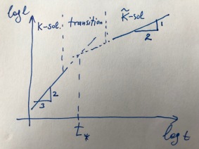
Figure 7: KGD fracture propagation in the toughness-dominated regime from early-time storage-dominated ($K$) to large-time leak-off-dominated ($\widetilde{K}$) regime.

2.3 Viscosity-dominated KGD propagation

In this case, the solid toughness is negligible compared to the dissipation in the viscous fluid flow. (We leave the task of quantifying the corresponding parametric regime for later). As in the toughness-dominated propagation in the above, let us focus first on the two sub-regimes, dominated by the storage in the fracture (negligible leak-off), which will call $M$-solution, and by the leak-off (negligible fluid storage in the fracture), which will call $\widetilde{M}$-solution, respectively. Intuitively, we expect that the former and the latter would actually define the early and large time behavior of the viscosity-dominated propagation.

2.3.1 Viscosity-storage-dominated ($M$) solution

As we have established from the fracture tip solution, the corresponding tip behavior is given by the storage–viscosity-dominated asymptote (12), $w\propto r^{2/3}$ and $p\propto-r^{-1/3}$ where the distance from the (right) tip $r=\ell(t)-x$. One can use a numerical method to find the complete solution for the KGD fracture in this regime, e.g. [22]. Instead, we will explore a simple analytical approximation of the $M$-solution, “inspired” by the $m$ tip asymptote, alone the lines of a more elaborate approach taken in [23, 24]. Specifically, we extend the opening tip asymptote to provide a consistent approximation for the entire KGD crack via replacing $r\Rightarrow(\ell^{2}-x^{2})/2\ell$, which (i) retains the tip asymptotic form in the limit $x\rightarrow\pm\ell$, and (b) allows for KGD crack symmetry and closure at both tips

$$w(x,t)\approx\delta_{m}\varphi(2/3)\,\ell_{m}^{1/3}\left(\frac{\ell^{2}-x^{2}}{2\ell}\right)^{2/3}$$ (32)

where $\delta_{m}\varphi(2/3)=2^{1/3}3^{5/6}$ is the numerical prefactor and the tip lengthscale $\ell_{m}$ is evaluated in terms of the instantaneous crack tip velocity $V=d\ell/dt$

$$\ell_{m}=\frac{\eta^{\prime}}{E^{\prime}}\frac{d\ell}{dt}$$ (33)

Corresponding approximation for the net-pressure can be evaluated from the crack elasticity integral (17). To complete the solution, we use the global fluid balance, which in the storage-dominated case with approximate opening given by (32) reduces to

$$Q_{o}t=V_{crack}=\int_{-\ell}^{+\ell}wdx\approx\frac{2^{1/3}3^{5/6}}{2^{2/3}}\,\ell_{m}^{1/3}\ell^{5/3}\int_{-1}^{+1}\left(1-\xi^{2}\right)^{2/3}d\xi=\alpha\,\ell_{m}^{1/3}\ell^{5/3}\quad\text{with}\quad\alpha\approx 2.93$$

(where $x/\ell$ was denoted as $\xi$ in the above opening integral). In view of (33), the above equation provides a simple ODE to solve for the crack half-length

$$\ell(t)\approx\underset{\gamma_{m}\approx 0.625}{\underbrace{\left(\frac{3}{2\alpha^{3}}\right)^{1/6}}}\underset{L_{m}(t)=\text{dynamic lengthscale}}{\underbrace{\left(\frac{E^{\prime}Q_{o}^{3}}{\eta^{\prime}}\right)^{1/6}t^{2/3}}}$$ (34)

This approximate solution satisfies all governing equations of the KGD crack with exception for the local (point-wise) fluid flow equation (only the global fluid balance, and not the local form, has been used in the construction of the solution). Notwithstanding, comparison with the accurate numerical solution of complete set of KGD equations for the non-dimensional crack length $\gamma_{m}=0.6152$ [22], shows a good agreement (1% error).

As already a familiar exercise, we can assess when does the storage-viscosity-dominated $M$-solution hold when the leak-off is non-negligible by evaluating $V_{leak@M}$ and comparing it with the injected volume. This predictably yields that the storage-dominated solution corresponds to the early time solution, when $t\ll t_{*}$, with the transition timescale given by ($V_{leak@M}(t_{*})\sim Q_{o}t_{*}$)

$$t_{*}=t_{M\rightarrow\widetilde{M}}=\frac{Q_{o}^{3}\eta^{\prime}}{C^{\prime 6}E^{\prime}}$$ (35)

2.3.2 Viscosity-leak-off-dominated ($\widetilde{M}$) solution

As we have established from the fracture tip solution, the corresponding tip behavior is given by the leak-off–viscosity-dominated asymptote (13), $w\propto r^{5/8}$ and $p\propto-r^{-3/8}$ where the distance from the (right) tip $r=\ell(t)-x$. Following the same route to the approximate $\widetilde{M}$-solution inspired by the tip asymptote, we write for the crack opening

$$w(x,t)\approx\delta_{\widetilde{m}}\varphi(5/8)\,\ell_{\widetilde{m}}^{3/8}\left(\frac{\ell^{2}-x^{2}}{2\ell}\right)^{5/8}$$ (36)

where $\delta_{\widetilde{m}}\varphi(5/8)$ is the numerical prefactor and the tip lengthscale $\ell_{\widetilde{m}}$ is evaluated in terms of the instantaneous crack tip velocity $V=d\ell/dt$

$$\ell_{\widetilde{m}}=\left(\frac{C^{\prime}\eta^{\prime}}{E^{\prime}}\right)^{2/3}\left(\frac{d\ell}{dt}\right)^{1/3}$$ (37)

Corresponding approximation for the net-pressure can be evaluated from the crack elasticity integral (17). To complete the solution, we use the global fluid balance, which in the leak-off-dominated case reduces to $Q_{o}t=V_{leak}$, which has been already solved for the crack -length evolution in the toughness-leak-off-dominated case in the above, with the solution given by

$$\ell(t)=\frac{1}{\pi}\frac{Q_{o}}{C^{\prime}}\sqrt{t}$$ (38)

This, in fact, suggests that the fracture evolution in the leak-off dominated case is irrespective of the solid vs. viscous fluid dissipation partition and given universally by the above expression. Substituting the crack length expression into $\ell_{\widetilde{m}}$ and the result into (36) completes the $\widetilde{M}$-solution.

Evaluating $V_{crack@\widetilde{M}}$ and comparing it with the injected volume renders the viscosity-leak-off-dominated $\widetilde{M}$-solution as a large time asymptote valid when $t\gg t_{*}$ with the transitional timescale defined by (35).

2.3.3 Summary of the viscosity-dominated propagation regime

The solution is given at the early ($t\ll t_{*})$ and large ($t\gg t_{*}$) time by the storage $M$- and leak-off $\widetilde{M}$- dominated asymptotes, while the transition from one to the other over $t\sim t_{*}$ can be computed numerically by solving the complete set of the KGD governing equations with $K^{\prime}=0$ [25, 20]. The transition timescale $t_{*}=t_{M\rightarrow\widetilde{M}}$ is given by (35).

2.4 General KGD solution, Parametric Space, and Perspective from the Tip

General KGD solution can be envisioned within the rectangular parametric space $M\widetilde{M}\widetilde{K}K$, Figure 8, with vertices corresponding to the above four limiting regime solutions, while the edges corresponding to the viscosity-dominated $M\widetilde{M}$ ($K^{\prime}=0$), toughness-dominated $K\widetilde{K}$ ($\eta^{\prime}$=0), storage-dominated $MK$ ($C^{\prime}=0$), and leak-off-dominated $\widetilde{M}\widetilde{K}$ ($C^{\prime}\rightarrow\infty$) regimes. [19, 20]

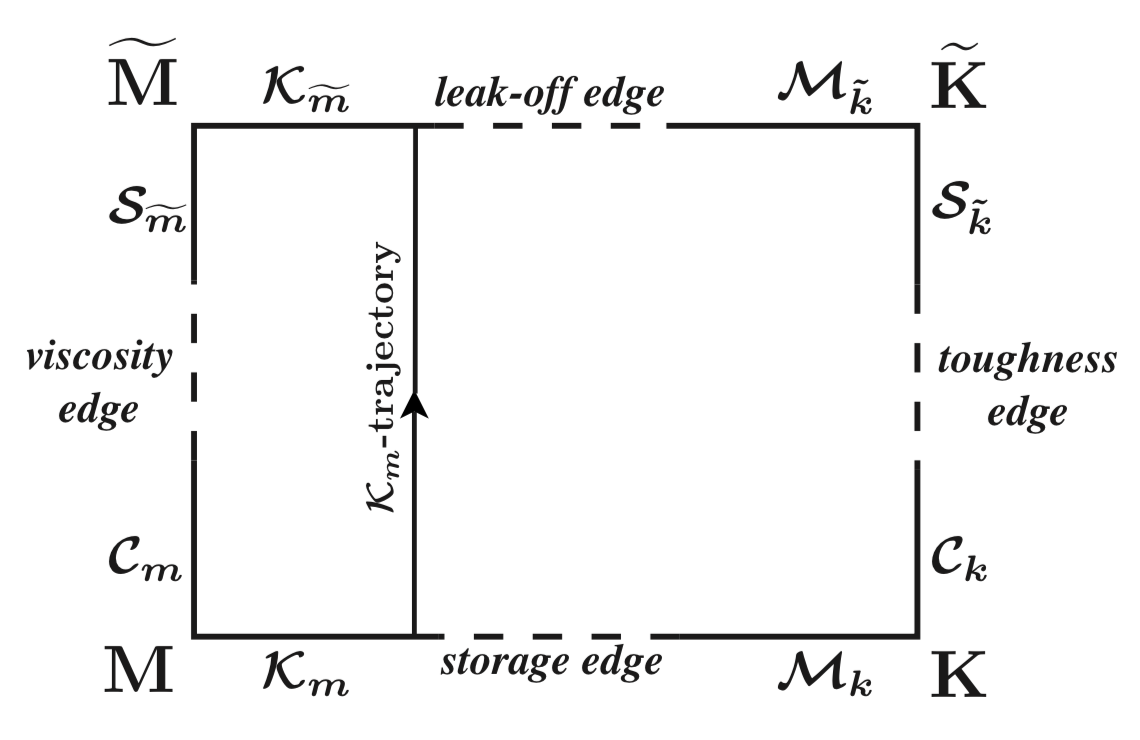
Figure 8: KGD fracture parametric space and a solution trajectory parametrized by, e.g., toughness number $K_{M}$ and leak-off number $C_{M}$, adopted from [20].

So far we have sketched-out the solution along the $M\widetilde{M}$ and the $K\widetilde{K}$ edges, corresponding to the fracture evolving from the storage to the leak-off dominated state over the transient timescale $t_{*}$ (given by $t_{M\rightarrow\widetilde{M}}$ and $t_{K\rightarrow\widetilde{K}}$, respectively). Thus, the solution trajectory along these two edges can be parametrized by corresponding normalized time $t/t_{*}$, which can alternatively be rewritten in terms of the the non-dimensional leak-off numbers

$$C_{M}=\left(\frac{t}{t_{M\rightarrow\widetilde{M}}}\right)^{1/6}=C^{\prime}\left(\frac{E^{\prime}\,t}{Q_{o}^{3}\eta^{\prime}}\right)^{1/6}\qquad C_{K}=\left(\frac{t}{t_{K\rightarrow\widetilde{K}}}\right)^{1/6}=C^{\prime}\left(\frac{E^{\prime 4}t}{Q_{o}^{2}K^{\prime 4}}\right)^{1/6}$$

Put in other words, the departure of the viscosity- (toughness-) dominated solution from the corresponding storage-dominated early time vertex $M$ ($K$) can be parametrized by the time-dependent leak-off number $C_{M}$ ($C_{K}$) - the quantifiable measure of the relative importance of the fracturing fluid leak-off vs. fluid storage in the KGD fracture.

Here we can relate this evolution of the KGD fracture to the evolution of its near tip field. Recall, for the viscosity-dominated case ($K^{\prime}=0$), that the HF tip solution corresponds to the transition with distance from the tip $r$ from the leak-off dominated near field $\widetilde{m}$-solution to the storage-dominated far field $m$-solution over the characteristic distance $r\sim\ell_{m\widetilde{m}}=C^{\prime 6}E^{\prime 2}/V^{5}\eta^{\prime 2}$. Intuitively, the finite fracture (KGD) fracture solution should be storage-dominated if that near tip transition can be accomplished within the scale of the finite fracture of half-length $\ell$, i.e. when $\ell_{m\widetilde{m}}\ll\ell$, and, leak-off dominated otherwise, when $\ell_{m\widetilde{m}}\gg\ell$. Evaluating the tip-to-global fracture lengthscale ratio $\ell_{m\widetilde{m}}/\ell$ assuming the storage-dominated KGD solution (34) for $\ell(t)$ and the corresponding crack tip velocity $V(t)=d\ell/dt$, we find (while dropping numerical prefactors of $O(1)$)

$$\left(\frac{\ell_{m\widetilde{m}}}{\ell}\right)_{@M}\sim C_{M}^{6}(t)$$

Since the non-dimensional leak-off number $C_{M}$ is increasing power law of time, we confirm the succession of the propagation regime in time from the storage to the leak-off dominated as seen from the perspective of the evolving fracture tip behavior corresponding to the dynamically expanding near tip transition lengthscale until it is no longer small compared to the finite fracture half-length $\ell$.

To glean the behavior along the energy dissipation axis of the parametric space (e.g. along the storage $MK$ edge of the parametric space), let us look at the storage-dominated tip solution corresponding to the transition from the toughness dominated near field $k$-solution to the viscosity-dominated far-field $m$-solution over the characteristic distance from the tip $r\sim\ell_{mk}=K^{\prime 6}/E^{\prime 4}V^{2}\eta^{\prime 2}$. Once again, the expectation is that the finite fracture solution is dominated by viscosity (viscous dissipation) if the near tip ($k$ to $m$) transition can be accomplished within the scale of the finite fracture half-length, i.e. when $\ell_{mk}\ll\ell$, and toughness-dominated otherwise, when $\ell_{mk}\gg\ell$. Evaluating the corresponding lengthscale ratio $\ell_{mk}/\ell$ assuming the viscosity-dominated ($M$) KGD solution (34) for $\ell(t)$ and $V(t)$, we find

$$\left(\frac{\ell_{mk}}{\ell}\right)_{@M}\sim K_{M}^{6}\qquad\text{with}\qquad K_{M}=\frac{K^{\prime}}{E^{\prime 3/4}Q_{o}^{1/4}\eta^{\prime 1/4}}$$

where $K_{M}$ has the meaning of the non-dimensional toughness reflecting the partition of energy dissipation between the solid and fluid. Similar exercise along the leak-off edge $\widetilde{M}\widetilde{K}$ of the parametric space results in comparing the near tip ($k$ to $\widetilde{m}$) transition lengthscale to the fracture half-length in the context of the viscosity-dominated ($\widetilde{M}$) KGD solution yields

$$\left(\frac{\ell_{\widetilde{m}k}}{\ell}\right)_{@\widetilde{M}}\sim K_{\widetilde{M}}^{6}\qquad\text{with}\qquad K_{\widetilde{M}}=K_{M}$$

Since $K_{M}$ (and $K_{\widetilde{M}}$) is time-independent, we conclude that the dissipation partition in the KGD fracture is time-invariant, and specifies a $K_{M}=const$ trajectory for a general KGD solution in the paramedic space, corresponding to the evolution of the propagating fracture from the early time storage to the large time leak-off dominated regime at a fixed dissipation partition.

2.5 Concluding remarks

We have focused on exploring the solution to the KGD (plane strain) hydraulic fracture and its parametric dependence in some details in the above. We showed that

• Approximate solutions in the limiting propagation regimes (when one fluid storage mechanism and one dissipation process dominate) can be effectively constructed from the corresponding near tip limiting solutions “adapted” to the finite fracture geometry and satisfying the global fluid balance equation

• In doing so, it is apparent that the near tip fracture behavior exerts the 1st order control on the overall solution of a finite HF

• The general finite HF solution can be represented as a trajectory in parametric space $M\widetilde{M}\widetilde{K}K$, defined by the four vertices corresponding to the above limiting regime solutions. The fracture evolves with time from the storage dominated to the leak-off dominated regime (tracked by the non-dimensional leak-off parameter $C_{M}\propto t^{1/6}$), while, for the KGD fracture, the dissipation partition between the solid (toughness) and the fluid (viscous friction losses in the fluid flow) dissipation is invariant (quantified by the time-independent non-dimensionless toughness parameter $K_{M}$)

• The non-dimensional leak-off $C_{M}$ and toughness $K_{M}$ parameters which instantaneous values define the current fracture propagation regime appear naturally when the dynamic HF tip transition lengthscale (e.g., in case of $C_{M}$,- $\ell_{m\widetilde{m}}$ for the transition with distance from the tip from the leak-off to storage dominated viscous regime) is compared to the lengthscale (half-length $\ell)$ of the finite fracture. So, once again the evolving structure of the near tip solution with changing fracture propagation velocity largely governs the evolution of the finite hydraulic fracture.

The radial (penny-shape) hydraulic fracture propagation from a point-fluid source can be treated in the similar manner to that of the KGD, once the crack elasticity and fluid flow equations are appropriately updated to the axisymmetric geometry. A general solution for the penny-shape HF can furnished in the same parametric space $M\widetilde{M}\widetilde{K}K$, with notable difference that, in this case, both the non-dimensional leak-off $C_{M}$ and the non-dimensional toughness $K_{M}$ are increasing power laws of time (e.g., [1]). This suggest that a general solution trajectory would start from the storage-viscosity and will end up in the leak-off-toughness dominated regime, as opposed to the KGD fracture propagation which preserves the dissipation partitioning.

References

- [1] E. Detournay. Mechanics of hydraulic fractures. Annu. Rev. Fluid Mech., 48(311-339), 2016.
- [2] ML Williams. Stress singularities resulting from various boundary conditions in angular corners of plates in extension. J. Appl. Mech., 19(4):526–528, 1952.
- [3] J.R. Barber. Elasticity, volume 172 of Solid Mechanics and its Applications. Springer, Dordrecht Heidelberg London New York, 3rd edition, 2010.
- [4] J. R. Rice. Mathematical analysis in the mechanics of fracture. In H. Liebowitz, editor, Fracture, an Advanced Treatise, volume II, chapter 3, pages 191–311. Academic Press, New York NY, 1968.
- [5] J. Desroches, E. Detournay, B. Lenoach, P. Papanastasiou, J. R. A. Pearson, M. Thiercelin, and A. H-D. Cheng. The crack tip region in hydraulic fracturing. Proc. Roy. Soc. London, Serie A(447):39–48, 1994.
- [6] B. Lenoach. The crack tip solution for hydraulic fracturing in a permeable solid. J. Mech. Phys. Solids, 43(7):1025–1043, 1995.
- [7] D. I. Garagash. Scaling of physical processes in fluid-driven fracture: Perspective from the tip. In F. Borodich, editor, IUTAM Symposium on Scaling in Solid Mechanics, volume 10 of IUTAM Bookseries, pages 91–100. Springer, 2009.
- [8] D. I. Garagash, E. Detournay, and J. I. Adachi. Multiscale tip asymptotics in hydraulic fracture with leak-off. J. Fluid Mech., 669:260–297, 2011.
- [9] F. Erdogan, G. D. Gupta, and T. S. Cook. Numerical solution of singular integral equations, volume 1 of Mechanics of Fracture, chapter 7, pages 368–425. Noordhoff International Publ., Leyden, 1973.
- [10] R. C. Viesca and D. I. Garagash. Numerical methods for coupled fracture problems. J. Mech. Phys. Solids, 113:13–34, 2018.
- [11] D. I. Garagash and E. Detournay. The tip region of a fluid-driven fracture in an elastic medium. ASME J. Appl. Mech., 67(1):183–192, 2000.
- [12] D. I. Garagash. Cohesive-zone effects in hydraulic fracture propagation. J. Mech. Phys. Solids, 133, December 2019.
- [13] M. Wrobel and G. Mishuris. Hydraulic fracture revisited: Particle velocity based simulation. Int. J. Eng. Sci., 94:23–58, 2015.
- [14] S.A. Khristianovic and Y.P. Zheltov. Formation of vertical fractures by means of highly viscous fluids. In Proc. 4th World Petroleum Congress, Rome, volume II, pages 579–586. Carlo Colombo Publishers, 1955.
- [15] J. Geertsma and F. de Klerk. A rapid method of predicting width and extent of hydraulic induced fractures. JPT, 246:1571–1581, 1969.
- [16] T. K. Perkins and L. R. Kern. Widths of hydraulic fractures. J. Pet. Tech., Trans. AIME, 222:937–949, 1961.
- [17] R. P. Nordgren. Propagation of vertical hydraulic fractures. J. Pet. Tech., 253:306–314, 1972. (SPE 3009).
- [18] Brice Lecampion, Andrew Bunger, and Xi Zhang. Numerical methods for hydraulic fracture propagation: A review of recent trends. Journal of natural gas science and engineering, 49:66–83, 2018.
- [19] E. Detournay. Propagation regimes of fluid-driven fractures in impermeable rocks. Int. J. Geomechanics, 4(1):1–11, 2004.
- [20] J. Hu and D. I. Garagash. Plane-strain propagation of a hydraulic fracture in a permeable rock with non-zero fracture toughness. ASCE J. Eng. Mech., 136(9):1152—1166, 2010.
- [21] A. P. Bunger, E. Detournay, and D. I. Garagash. Toughness-dominated hydraulic fracture with leak-off. Int. J. Fracture, 134:175–190, 2005.
- [22] J. I. Adachi and E. Detournay. Self-similar solution of a plane-strain fracture driven by a power-law fluid. Int. J. Numer. Anal. Methods Geomech., 26:579–604, 2002.
- [23] E. V. Dontsov. An approximate solution for a penny-shaped hydraulic fracture that accounts for fracture toughness, fluid viscosity and leak-off. R. Soc. open sci., 3:160737, 2016.
- [24] E. V. Dontsov. An approximate solution for a plane strain hydraulic fracture that accounts for fracture toughness, fluid viscosity, and leak-off. Int. J. Fracture, 205(2):221–237, 2017.
- [25] J. I. Adachi and E. Detournay. Plane-strain propagation of a hydraulic fracture in a permeable rock. Engng. Fract. Mech., 75:4666–4694, 2008.