An implimentation of the Differential Filter
for Computing Gradient and Hessian
of the Log-likelihood of Nonstationary Time Series Models
Genshiro Kitagawa
Mathematics and Informatics Center, The University of Tokyo
Abstract
The state-space model and the Kalman filter provide us with unified and computationaly
efficient procedure for computing the log-likelihood of the diverse type of time series models.
This paper presents an algorithm for computing the gradient and the Hessian matrix of the log-likelihood
by extending the Kalman filter without resorting to the numerical difference.
Different from the previous paper [13],
it is assumed that the observation noise variance .
It is known that for univariate time series, by maximizing the log-likelihood of this restricted model,
we can obtain the same estimates as the ones for the original state-space model.
By this modification, the algorithm for computing the gradient and the Hessian becomes
somewhat complicated. However, the dimension of the parameter vector is reduce by one
and thus has a significant merit in estimating the parameter of the state-space model
especially for relatively low dimentional parameter vector.
Three examples of nonstationary time seirres models, i.e., trend model, statndard
seasonal adjustment model and the seasonal adjustment model with AR componet are presented to
exemplified the specification of structural matrices.
1 Introduction: The Maximum Likelihood Estimation of a State-Space Model
We consider a linear Gaussian state-space model
(1)
(2)
where is a one-dimensional time series, is an -dimensional state vector, is a -dimesional Gaussian white noise, , and is a one-dimensional white noise, .
, and are matrix, matrix and vector. respectively.
is the -dimensional parameter vector of the state-space model such as the variances of the noise
inputs and unknown coefficients in the matrices , , and .
For simplicity of the notation, hereafter, the parameter and the suffix will be omitted.
It is noted that for the state-space model of the univariate time series, the assumption that does not
lose any genrality, since it is known that even with this assumption we can obtaine the same estimates of the
parameters of the model by a proper transformation (Kitagawa (2020)).
Various models used in time series analysis can be treated uniformly within the state-space model framework.
Further, many problems of time series analysis, such as prediction, signal extraction, decomposition, parameter estimation and interpolation, can be formulated as the estimation of the state of a state-space model.
Given the time series and the state-space model (1)
and (2), the one-step-ahead predictor and the filter and their variance covariance
matrices and are obtained by the following Kalman filter (Anderson and Moore (2012) and Kitagawa (2020)):
One-step-ahead prediction
(3)
Filter
(4)
Given the data , the likelihood of the time series model is defined by
(5)
where is the conditional distribution of given the observation and is a normal distribution given by
(6)
where and are the one-step-ahead prediction error and
its variance defined by
(7)
Therefore, the log-likelihood of the state-space model is obtained as
(8)
where the maximum likelihood estimate of the variance is given by
(9)
The maximum likelihood estimates of the parameters of the state-space model
can be obtained by maximizing the log-likelihood function (8).
In general, since the log-likelihood function is mostly nonlinear, the maximum likelihood estimates are obtained by using a numerical optimization algorithm based on the quasi-Newton method.
According to this method, using the value of the log-likelihood and the first derivative (gradient) for a given parameter , the maximizer of is automatically estimated by repeating
(10)
where is an initial estimate of the parameter.
The step width is automatically determined and the inverse matrix of the Hessian matrix is obtained recursively by the DFP or BFGS algorithms (Fletcher (2013)).
Here, the gradient of the log-likelihood function is usually approximated by numerical difference,
such as
(11)
where is defined by , for some small such as 0.0001.
The numerical difference usually yields reasonable approximation to the gradient of the
log-likelihood.
However, since it requires times of log-likelihood evaluations, the amount of computation
becomes considerablly large if the dimension of the parameters is large.
Further, if the the maximum likelihood estimates lie very close to the boundary of
addmissible domain, which sometimes occure in regularization problems,
it becomes difficult to obtain the approximation to the gradient of the log-likelihood
by the numerical difference.
Analytic derivative of the log-likelihood of time series models were considered by many authors.
For example, Kohn and Ansley (1985) gave method for computing likelihood and its derivatives for an ARMA model.
Zadrozny (1989) derived analytic derivatives for estimation of linear dynamic models.
Kulikova (2009) presented square-root algorithm for the evaluation of the likelihood gradient to avoid numerical instability of the recursive algorithm for log-likelihood computation.
In this paper, the gradient and Hessian of the log-likelihood of linear state-space model are given
under the assumption that the observation noise variance is 1.
By this method, the dimension of the unknown parameter is reduced by one, but instead
the derivative of the observation noise variance must be computed simultaneously.
Details of the implementation of the algorithm for the trend model, the standard seasonal adjustment model and the seasonal adjustment model with stationary AR component are given.
For each implementation, comparison with a numerical difference method is shown.
In section 2, algorithm for obtaining the gradient and the Hessian of the log-likelihood
is presented.
Application of the method is exemplified with the three models, i.e., the trend model, the standard seasonal adjustment model and the seasonal adjustment model
with autoregressive component are shown in section 3.
2 The Gradient and the Hessian of the log-likelihood
The recursive algorithm for computing the gradient and the Hessian of the
log-likelihood is essentially the same as the one shown in Kitagawa(2020b).
However, we assume that the observation noise variance is 1, the expression
for the gradient and the Hessain matrix become simple.
Instead, we need to evaluate the first and the second derivative of the
observation noise variance .
2.1 The gradient of the log-likelihood
From (8), the gradient of the log-likelihood is obtained by
(12)
where, from (7) and (9), the derivatives of the one-step-ahead predition , the
one-step-ahead prediction error variance and the observation
noise variance are obtained by
(13)
(14)
(15)
To evaluate these quantities, we need the derivatives of the one-step-ahead predictor
of the state and its variance covariance
matrix which can be obtained recursively
in parallel to the Kalman filter algorithm:
[One-step-ahead-prediction]
(16)
[Filter]
(17)
2.2 Hessian of the Log-likelihood of the State-space Model
The Hessian (the second derivative) of the log-likelihood can
also be obtained by a recursive formula,
since, from (12), it is given as
To evaluate the Hessian, the following computation should be performed
along with the recursive formula for the log-likelihood and the
gradient of the log-likelihood.
(21)
3 Examples
In order to implement the differential filter, it is necessary to to specify
the first and the second derivatives
of , , and along with the original state-space model.
In this section, we shall consider three typical cases.
The first two examples are the trend model and the standard seasonal adjeustment model,
for which three matrices (or vectors), , and do not contain unknown
parameters and thus the derivatives
of these matrics becomes 0.
This makes the algorithm for the gradient and the Hessian of the log-likelihood
presented in the previous section considerablly simple.
The third example is the seasonal adjustment model with AR component.
For this model, the matrix depends on the unknown AR coefficients,
although the derivative of is very sparse.
However, since we usually use a nonlinear transformation of the parameters
and the Levinson’s formula between partial autocorrelations coefficients
and AR coefficients, to ensure the stationarity condition,
the expression of the non-zero elements of the derivatives of becomes fairly complex.
3.1 Trend model
The trend model is a typical example of the case where only the noise covariance
depends on the unknown parameter .
Consider a trend model
(22)
where is the trend component
that typically follow the following model
(23)
where is the back-shift operator satisfying ,
and are assumed to be Gaussian white noise with
variances and , respectively (Kitagawa and Gersch (1984,1996) and
Kitagawa (2020a)).
Note that for and , the model (23) becomes
and , respectively,
and that in the Kalman filter, the essentially the same filtering
results can be obtained by assuming that (Kitagawa (2020a))
and thus the dimension of the unknown parameter vector is reduced by one,
i.e., in the case of the trend model the dimension of the parameter
becomes one.
This trend model can be expressed in
the state-space model form as
(24)
with and and the state vector and
the matrices , , , and are defined by
(25)
for and
(32)
(34)
for .
In this state-space representation, the parameter is ,
and the , , and do not depend on the parameter.
Therefore, we have
and .
In actual likelihood maximization, since there is a positivity
constraint, ,
it is frequently used a log-transformation,
(35)
and maximize the log-likelihood with respect to this transformed parameter .
In this case,
(36)
Since log-transfomation is a monotone incresing function, we can get the
same parameter by solving this modified optimization problem.
In this case, the recursive algorithm for gradient of the log-likelihood
becomes significantly simple as follows:
(37)
where, from (7), the derivatives of the one-step-ahead predition error , the
one-step-ahead prediction error variance and the observation noise variance
are obtained by
(38)
(39)
The formula for obtaining the derivatives of the state and its variance covariance matrix become
The Hessian (the second derivative) of the log-likelihood is also obtained
by a recursive formula, since, from (12), it is given as
Therefore, to evaluate the Hessian, the following computation should be performed
along with the recursive formula for the log-likelihood and the
gradient and Hessian of the log-likelihood.
Note that since in this example, the parameter is one dimentional,
we should read in the following formula.
(42)
Table 1: Comparison of the results by the numerical diffference and the proposed analytic method for the first order trend model (). Left: initial values, Right: final estimate.
Difference
Analytic
Difference
Analytic
0.50000
0.50000
4.49933
4.49933
1.50393
1.50393
317.9243
317.9243
9.87647
9.87647
For Whard (whole sale hardware) data (Kitagawa (2020a)), ,
the system noise variance parameter of the trend model
with was estimated using the initial value , i.e., .
By a numerical optimization procedure the maximum likelihood estimate of the parameter is obtained
as , i.e., .
Table 1 shows the log-likelihoods, the gradients, the Hessians and the
observation noise variances of the initial and the final estimates.
For comparison, the values obtained by the numerical difference are also shown in the table.
The log-likelihood of the model with these initial and final estimates are
and , respectively.
It can be seen that the analytic gradient and the Hessian coincide with ones obtained by the numerical differentiation at least up to 4th digit.
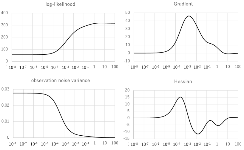
Figure 1: The log-likelihood, the gradient, the Hessian and the variance of the observation
noise of the trend models with order 1. The horizontal axes are the value of the system noise
variance in log-scale.
Figure 1 shows the change of the log-likelihood, the gradient,
Hessian and the observation noise variance for various values of the system noise vaiance
.
In this case, the log-likelihood has only one local maximum and the gradient is unimodal.
On the other hand, the Hessian has two peakes and two troughs.
Table 2: Comparison of the results by the numerical diffference and the proposed analytic method for the second order trend model ()
Difference
Analytic
Difference
Analytic
-0.53318
-0.53318
0.58674
0.58674
-270.02065
-270.02065
296.17899
296.17899
1.68866
1.68866
0.010951
0.010953
-6.150639
-6.15072
-283.72502
-283.72502
283.73930
283.73930
-0.214378
-0.21437
-1.58184
-1.58183
-1.66045
-1.66045
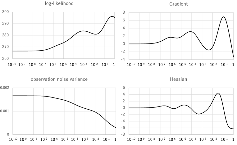
Figure 2: The log-likelihood, the gradient, the Hessian and the variance of the observation
noise of the trend models with order 2. The horizontal axes are the value of the system noise
variance in log-scale.
Table 2 shows the results for the sencond order trend model.
In this case, the final estimate obtained by the numerical optimization procedure
depends on the initial estimate and two cases are shown in the table.
If the inital estiamte is set to , i.e., , the final estimate is , i.e.,
with the log-likelihood value .
On the other hand, if we set the initial estimate as , i.e., , the final
estiamte becomes , i.e., with .
Comparing the log-likelihodd values, is the maximum likelihood
estimate of the second order trend model.
Figure 2 shows the change of the log-likelihood, the gradient,
the Hessian and the observation noise variance for various values of the system noise vaiance
for the second order trend model.
In this case, the log-likelihood is bimodal and the gradient attains zero at three points,
two local maxima and one local minimum.
The Hessian of the two local maximum likelihood estiamte, 0.58674 and
are 6.15072 and 1.66045, respectively.
This indicates that the estimate 0.58674 has sharper peak in the log-likelihood function.
3.2 The standard seasonal adjustment model
As the second example, we consider a standard seasonal adjustment model
(43)
where and are the trend component and the seasonal component
that typically follow the following model
(44)
The noise terms , and are assumed to be Gaussian white noise with
variances , and , respectively (Kitagawa and Gersch (1984,1996) and
Kitagawa (2020a)).
This seasonal adjustment model with two component models can be expressed in
state-space model form as
(45)
with and and the state vector and
the matrices , , , and are defined by
(64)
(66)
(69)
It is noted that, similar to the trend model, it is possible to assume
that .
In this case, the parameter is ,
and the , , and do not depend on the parameter.
In actual likelihood maximization, since there are positivity
constrains, and ,
we use the log-transformation,
(70)
In this case,
(77)
(78)
Since , and do not depend on and ,
and hold,
we can use the same recursive algorithm for gradient and the Hessian of the log-likelihood
as the one for the trend model.
For Whard data, the standard seasonal adjustment model with , is estimated
using the initial estimates of parameters,
.
The log-likelihood of the model with these initial parameters is
and the gradient and the Hessian obtained by the numerical difference and the proposed
method are shown in the Table 3.
It can be seen that the numerical differentiation coincides with the analytic
derivative up to 5th digit.
The maximum likelihood estimates of the system noises are ,
with .
Table 3: Comparison of the results by numerical diffference and the differential filter
Proposed method
Numerical Difference
Initial
Optimized
380.6569
380.6569
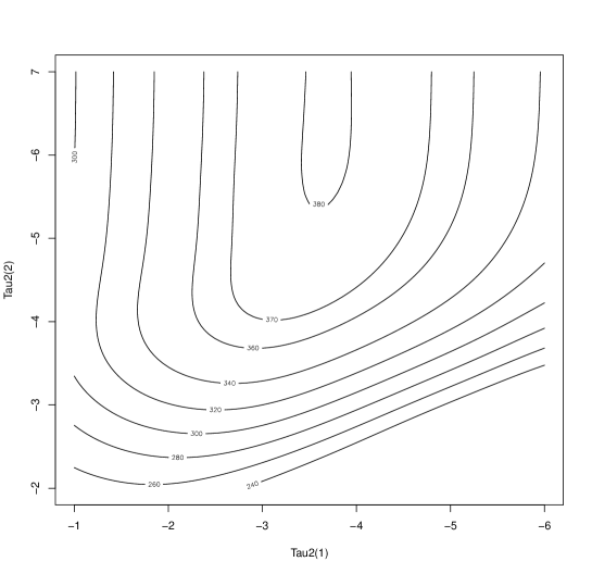
Figure 3 shows the contour of the log-likelihood of the seasonal adjustment model.
The horizontal and the vertical axes indicate the common logarithms of and
, respectively.
The log-likelihood has a similar values for smaller and form a platou.
The small value of ,
0.18135, corresponds to this phenomenon.
Figure 3: Contour of log-likelihood function of seasonal adjustment model. Horizontal zxis: common logatithm of ,
Vertical axis: common logarithm of .
3.3 Seasonal adjustment model with stationary AR component
The third example is a seasonal adjustment model with statinary AR component
(79)
where and are the trend component and the seasonal component
introduced in the previous subsection and is an AR component with AR order defined by
(80)
Here is a Gaussian white noise with variance .
The model contains parameters and the parameter vector is given by
.
The matrices , , , and are defined by
(111)
(113)
(117)
The relation between the parameter and the variances and AR coefficients
are as follows.
(118)
(119)
Note that the equation (119) is the relation between the AR coefficients
of order and those of the order used in the Levinson’s algorithm (Kitagawa (2020a)).
In this case,
(126)
(133)
(134)
(139)
(144)
where and
denote the components
of the matrices and
,
respectively, and
and
are obtained by
(145)
(146)
and
(149)
(152)
(157)
(161)
In the above equations, and are the first and the second derivatives
of the nonlinear transformation
and are given by
(162)
For , , the matrices ,
, ,
,
and
are given by
(173)
(184)
where for , 2 and 3, and
are respectively give by:
For
For
(187)
(192)
(197)
(202)
For ,
(208)
(218)
(228)
(238)
(248)
Since we have
and
for the current model, the differential filter shown in
(12)-(21) become considerably simple as follows.
[The gradient of the log-likelihood]
(249)
where
(250)
(251)
[The derivative of the one-step-ahead predictor and the filter]
(252)
(253)
[The Hessian of the log-likelihood]
where ,
and are
obtained by
(254)
[The second derivatives of the one-step-ahead predictor and the filter]
(255)
Table 4: Comparison of the gradient vectors and the Hessian matrix obtained by
the differential filter and the numerical differencing.
By differential filter:
3.472775
3.244577
21.235746
4.505459
0.320932
1.233847
1.233847
5.956742
7.917642
0.399997
5.956742
7.917642
11.233390
0.822854
0.399997
0.822854
3.126537
By numerical differencing:
3.472775
3.244577
21.235747
4.505459
0.320913
1.233881
1.233881
5.956570
7.917585
0.400087
5.956570
7.917585
0.822888
0.400087
0.822888
3.126465
Table 4 shows the gradients and the Hessian matrix obtained by
the differential filter and the numerical differenting method.
The initial estimates of the parameters are set to be
and the log-likelihood of the model is
= .
The maximum likelihoos estimates of the model are ,
, ,
and with = 387.9554.
The gradients and the Hessian matrix for this maximum likelihood estimates are shown in
Table 5.
In this case as well, the analytic derivative matches the numerical differentiation up to the fifth digit.
Table 5: Comparison of the gradient vectors and the Hessian matrix obtained by
the differential filter and the numerical differencing.
By differential filter:
0.000001
0.000007
0.000000
0.036523
0.029211
0.036523
0.371657
0.000000
0.371657
7.186088
0.000000
0.029211
7.186088
By numerical differencing:
0.000002
0.000011
0.000003
0.036524
0.029217
0.036524
0.371642
0.000001
0.371642
7.186086
0.000001
0.000002
0.029217
7.186086
0.000002
4 Summary
The gradient and the Hessian matrix of the log-likelihood of the reduced order linear state-space
model are given.
Details of the implementation of the algorithm for trend model, the standard seasonal adjustment model,
and the seasonal adjustment model with stationary AR component are given.
For each implementation, comparison with a numerical difference method is shown.
Aknowledgements
This work was supported in part by JSPS KAKENHI Grant Number 18H03210.
The author is grateful to the project members, Prof. Kunitomo, Prof Nakano,
Prof. Kyo, Prof. Sato, Prof. Tanokura and Prof. Nagao for their
stimulating discussions.
References
[1]
[2]Akaike, H. (1980b), “Seasonal adjustment by a Bayesian modeling”, J. Time Series Anal., 1, 1–13.
[3]
[4]Akaike, H. and Ishiguro, M. (1983), “Comparative study of X-11 and Bayesian procedure of seasonal adjustment,” Applied Time Series Analysis of Economic Data, U.S. Census Bureau.
[5]
Anderson, B. D. O, and Moore, J. B. (2012). Optimal filtering. DOver Publications, New York.
[6]Box, G.E.P., Hillmer, S.C. and Tiao, G.C. (1978) “Analysis and modeling of seasonal time series”, in Seasonal Analysis of Time Seres, ed.Zellner, A., US Bureau of the Census, Economic Research Report ER-1, 309–334.
[7]
Fletcher, R. (2013). Practical methods of optimization. John Wiley & Sons.
[8]
Kitagawa, G. (1987). Non-Gaussian state-space modeling of nonstationary time series.
Journal of the American Statistical Association, 82(400), 1032–1041.
[9]
Kitagawa, G. (1989). Non-Gaussian seasonal adjustment, Computers & Mathematics with Applications,
Vol.18, No.6/7, pp. 503–514.
[10]
Kitagawa, G. (1994). The two-filter formula for smoothing and an implementation of the Gaussian-sum smoother,
Annals of the Institute of Statistical Mathematics, Vol. 46, No.4, pp. 605–623.
[11]
Kitagawa, G. (1996). Monte Carlo filter and smoother for non-Gaussian nonlinear state space models,
Journal of Computational and Graphical Statistics, Vol.5, no.1, pp. 1–25.
[12]
Kitagawa, G. (2020a). Introduction to Time Series Modeling with Applications in R,
Monographs on Statistics and Applied Probability 166, CRD Press, Chapman & Hall, New York.
[13]
Kitagawa, G. (2020b). Computation of the Gradient and the Hessian of the Log-likelihood of the State-space Model by the Kalman Filter, arXiv preprint arXiv:2011.09638.
[14]
Kitagawa, G. and Gersch, W. (1984), “A smoothness priors-state space modeling of
time series with trend and seasonality”, J. Amer. Statist. Assoc., 79, 378–389.
[15]Kitagawa, G. and Gersch, W. (1996), Smoothness Priors Analysis of Time Series,
Lecture Notes in Statistics, 116, Springer, New York.
[16]
Kohn, R., and Ansley, C. F. (1985). “Computing the likelihood and its dierivatives for a gaussian ARMA model”. Journal of Statistical Computation and Simulation, 22(3-4), 229–263.
[17]
Konishi, S. and Kitagawa, G. (2008), Information Criteria and Statistical Modeling, Springer Series in Statistics, pp-273, Springer, New York.
[18]
Kulikova, M. V. (2009). “Likelihood Gradient Evaluation Using Square-Root Covariance Filters”,
IEEE Transactions on Automatic Control, Vol. 54, Issue 3, 646-651.
[19]
Takeuchi, K. (1976). “Distributions of information statistics ans criteria for adequacy of models”, Mathematical Science, 1553, 12–18 (in Japanese).
[20]
Zadrozny, P. A. (1989). “Analytic derivatives for estimation of linear dunamic models”,
Computers Math. Applic., Vol. 18, No. 6/7, 539-553.