Estimating the entanglement of
random multipartite quantum states

Abstract

Genuine multipartite entanglement of a given multipartite pure quantum state can be quantified through its geometric measure of entanglement, which, up to logarithms, is simply the maximum overlap of the corresponding unit tensor with product unit tensors, a quantity that is also known as the injective norm of the tensor. Our general goal in this work is to estimate this injective norm of randomly sampled tensors. To this end, we study and compare various algorithms, based either on the widely used alternating least squares method or on a novel normalized gradient descent approach, and suited to either symmetrized or non-symmetrized random tensors. We first benchmark their respective performances on the case of symmetrized real Gaussian tensors, whose asymptotic average injective norm is known analytically. Having established that our proposed normalized gradient descent algorithm generally performs best, we then use it to obtain numerical estimates for the average injective norm of complex Gaussian tensors (i.e. up to normalization uniformly distributed multipartite pure quantum states), with or without permutation-invariance. Finally, we also estimate the average injective norm of random matrix product states constructed from Gaussian local tensors, with or without translation-invariance. All these results constitute the first numerical estimates on the amount of genuinely multipartite entanglement typically present in various models of random multipartite pure states.

1 Introduction

In quantum information theory, the notion of entanglement [HHHH09] plays a central role, providing the framework in which purely quantum correlations are described. Bipartite entanglement, i.e. the quantum correlations between two parties, has received a lot of attention in the literature, with a rather simple characterization in the case of pure states, in terms of the entropy of entanglement. The case of multipartite entanglement, i.e. quantum correlations shared by three or more parties, is qualitatively more complicated. The geometry of the set of pure entangled states is much richer in this case [DVC00], and there are several inequivalent ways to measure how much entanglement is present in a given multipartite pure quantum state [CKW00, BL01, WC01].

Among the measures of multipartite pure state entanglement discussed in the literature, the geometric measure of entanglement introduced in [BL01] has a natural and geometrical definition: it is the (negative logarithm of the) maximum overlap between the given quantum state and any product state. From a mathematical standpoint, this quantity is nothing but the injective tensor norm of the corresponding tensor [Gro56, Rya13, AS17]. The latter quantity is the focus of this work: we discuss several numerical algorithms to compute it, in particular for various models of random multipartite pure states.

Random quantum states have found several applications in quantum information theory [CN16], ranging from the characterization of the entanglement of mixed bipartite states [ASY14] to the solutions of important conjectures in quantum Shannon theory [Has09]. In this work, we are concerned with the entanglement of random pure states. The uniform probability distribution on the set of pure states corresponds to the uniform probability distribution on the unit sphere of a complex Hilbert space [ŻPNC11]. Here, we are interested in the case where the total Hilbert space admits a tensor product structure with three or more factors. Understanding the amount of entanglement (via the geometric measure) for such random pure states tells us what is the entanglement of a typical multipartite pure quantum state, and it is this random variable that we aim to study in this work. We are also interested in estimating the entanglement of random matrix product states (MPS), again using a natural probability measure on the set of MPS with given local dimensions [GdOZ10, CGGPG13, GGJN18, LPG22, HBRE21].

As is the case with most questions related to tensors, computing the geometric measure of entanglement, or equivalently the injective norm, is a computationally difficult (NP-hard) question [HL13]. We tackle this problem with various numerical algorithms, obtaining lower bounds on both quantities by finding good candidates for product states having large overlaps with the input tensor. We compare the widely used alternating least squares algorithm [Har70] with our proposed normalized gradient descent based algorithm, which incorporates normalization at each step. We benchmark these algorithms on random tensors, with or without symmetry. In the symmetric case, we also test the symmetrized counterparts of these algorithms. We choose symmetrized real Gaussian tensors as the initial benchmark owing to the presence of analytical results for the large dimensional asymptotic limits of their injective norms [ABAČ13, PWB20]. We notice that the numerical results closely match the analytical values. In the other cases (symmetrized complex tensors and non-symmetrized real and complex tensors), our numerical estimates for the injective norm of typical tensors provide the first approximate values for the elusive almost-sure limit values. We observe that the values we obtain match asymptotic lower and upper bounds in the large dimension and/or number of tensor factors limits. We study the effect of symmetrization on the value of the geometric measure of entanglement, showing that symmetrized tensors are less entangled than their non-symmetrized counterparts. We also fit simple functions encoding the asymptotic value and first order corrections on the numerical values obtained using the normalized gradient descent algorithm.

We then study, for the first time, the genuinely multipartite entanglement of random matrix product states (MPS) using the numerical algorithms that we develop. Up to now, the main focus in the random MPS literature was the understanding of their bipartite entanglement or correlations, over a bipartition that respects the tensor network structure [GdOZ10, CGGPG13, GGJN18, HBRE21, LPG22]. The novelty of our work is to derive numerical results about the typical multipartite entanglement of such states that are of paramount importance in theoretical physics and condensed matter theory. We compare these values to the ones of Gaussian tensors, showing agreement in the limit of large bond dimension. We also study the effect of (partial) symmetrization on the entanglement of the states.

The paper is organized as follows. In Section 2, we introduce the injective norm, its basic properties, and its relation to the quantification of multipartite entanglement via the geometric measure of entanglement (GME). In Section 3, we give a detailed exposition of the main numerical algorithms used to approximate the injective norm of arbitrary tensors, and we propose a new algorithm, called normalized gradient descent (NGD), as well as its symmetrized version. Then in Section 4, we benchmark these algorithms on random real Gaussian tensors, with and without permutation symmetry. Having established that our proposed NGD algorithm is the most performant, we then use it, in Section 5, to estimate the injective norm of random uniformly distributed multipartite pure quantum states (i.e. normalized random complex Gaussian tensors), again with or without permutation symmetry. Finally, in Section 6, we study the injective norm of random matrix product states in different scenarios, with or without translation-invariance, and asymptotic regimes (large physical and/or bond dimension). In Appendix A, we present additional benchmarking results for the different algorithms obtained by running them on deterministic states whose value of GME is known. In addition, we provide open access to our code containing the proposed algorithms, which can be deployed on any tensor (with any number of tensor factors and any local dimensions) [FLN22].

2 The injective norm and the geometric measure of entanglement

The extent to which a multipartite pure state is entangled can be estimated by the angle it makes with the closest pure product state. The injective norm of a tensor $\Psi\in\mathbb{C}^{d_{1}}\otimes\mathbb{C}^{d_{2}}\otimes\cdots\otimes\mathbb{C}^{d_{n}}$ is defined as

$$\|\Psi\|_{\varepsilon}=\max_{\phi\in\operatorname{PRO}}\mid\langle\Psi|\phi\rangle\mid,$$ (1)

where $\operatorname{PRO}$ is the set of all product states in $\mathbb{C}^{d_{1}}\otimes\mathbb{C}^{d_{2}}\otimes\cdots\otimes\mathbb{C}^{d_{n}}$, i.e. product tensors with Euclidean norm equal to $1$ in $\mathbb{C}^{d_{1}}\otimes\mathbb{C}^{d_{2}}\otimes\cdots\otimes\mathbb{C}^{d_{n}}$. Further, the normalized injective norm of $\Psi$ is the ratio of its injective norm to its Euclidean norm and is equal to the injective norm of the normalized tensor $\hat{\Psi}=\Psi/\|\Psi\|$, where $\|\cdot\|$ denotes the Euclidean norm.

$$\|\hat{\Psi}\|_{\varepsilon}=\frac{\|\Psi\|_{\varepsilon}}{\|\Psi\|}$$ (2)

The geometric measure of entanglement (GME) [Shi95, BL01, WG03, ZCH10] is defined as the negative logarithm of $\|\hat{\Psi}\|_{\varepsilon}^{2}$. It is a faithful measure of entanglement for multipartite pure states as it is equal to $0$ if and only if $\hat{\Psi}$ is a product state.

$$\operatorname{GME}(\Psi)=-\log_{2}\left(\|\hat{\Psi}\|_{\varepsilon}^{2}\right)=-\log_{2}\left(\frac{\|\Psi\|_{\varepsilon}^{2}}{\|\Psi\|^{2}}\right)$$ (3)

Let us also point out that computing the injective norm of a tensor is equivalent to finding its closest product state approximation. Consider the objective of finding the closest product state $\phi\in\operatorname{PRO}$ of a tensor $\Psi\in\mathbb{C}^{d_{1}}\otimes\mathbb{C}^{d_{2}}\otimes\cdots\otimes\mathbb{C}^{d_{n}}$.

$$\min_{\phi\in\operatorname{PRO}}\|\Psi-\phi\|^{2}=\min_{\phi\in\operatorname{PRO}}\left(\|\Psi\|^{2}+\|\phi\|^{2}-\langle\Psi|\phi\rangle-\langle\phi|\Psi\rangle\right)=\min_{\phi\in\operatorname{PRO}}\left(\|\Psi\|^{2}+1-\langle\Psi|\phi\rangle-\langle\phi|\Psi\rangle)\right)$$ (4)

Since $\|\Psi\|$ is fixed for an initial choice of $\Psi$, the minimization objective is equivalent to maximizing the inner product between $\Psi$ and the product state approximation $\phi$. Which in turn, is equivalent to the definition of the injective norm $\|\Psi\|_{\varepsilon}$ from Equation (1).

$$\min_{\phi\in\operatorname{PRO}}\|\Psi-\phi\|^{2}\equiv\|\Psi\|^{2}+1-2\max_{\phi\in\operatorname{PRO}}|\langle\Psi|\phi\rangle|=1+\|\Psi\|^{2}-2\|\Psi\|_{\varepsilon}$$ (5)

Let us make one last comment about this injective norm. Note that, if $n=2$, then $\|\Psi\|_{\varepsilon}$ is simply the largest Schmidt coefficient of $\Psi\in\mathbb{C}^{d_{1}}\otimes\mathbb{C}^{d_{2}}$ (or equivalently the largest singular value or operator norm, if viewed as an element of $\mathcal{M}_{d_{1}\times d_{2}}(\mathbb{C})$). It is thus a particularly easy quantity to compute. However, the picture changes drastically for higher order tensors: already for $n=3$, $\|\Psi\|_{\varepsilon}$ is, in general, difficult to estimate, both analytically (NP-hard) and numerically [HL13].

3 Algorithms for approximating the injective norm of tensors

In this section, we briefly explain the algorithms that we employ for finding the closest product state approximation of a tensor.

3.1 Alternating least squares

The alternating least squares (ALS) [Har70] algorithm tries approximating a tensor $\Psi$ as a sum of $R$ rank one tensors. The vectors $a^{(i)}_{r}\;\forall\;i\in\{1,2,\ldots,n\}$ involved in calculating the rank one tensors are called cores.

$$\phi=\sum_{r=1}^{R}a^{(1)}_{r}\otimes a^{(2)}_{r}\otimes\cdots\otimes a^{(n)}_{r}$$ (6)

As the name suggests, ALS focuses on iteratively optimizing the cores in a way that optimizes the squared error loss between specific views of the approximation and the original tensor [Har70]. Since ALS considers only one view of the original tensor at a time, it does not preserve the structure of the tensor during optimization. Further, ALS does not restrict $\|\phi\|$ during the optimization process, so $\|\phi\|$ grows in proportion to $\|\Psi\|$, and it is thus needed to normalize the result post-convergence $\hat{\phi}=\frac{\phi}{\|\phi\|}$.

3.2 Power iterations method

The power iterations method (PIM) [Evn21] is a symmetrized version of ALS that approximates a symmetric tensor as a sum of $R$ symmetric rank one tensors. However, unlike ALS, it considers normalization on each step of optimization. Although this eradicates the need for explicitly normalizing the approximation post-convergence, the value of $\|\phi\|$ at each step of the optimization process depends on the value of $\|\Psi\|$. Hence, upon normalizing $\phi$ on the last step of optimization, PIM induces a similar norm scaling situation as with ALS.

$$\hat{\phi}=\sum_{r=1}^{R}\hat{a}_{r}^{\otimes n}$$ (7)

3.3 Normalized gradient descent

Although ALS is widely used and is even shown to perform better than gradient descent for finding finite rank approximations of tensors [CLDA09], it does not consider normalization implicitly. We develop a novel normalized gradient descent (NGD) algorithm as a modification of the projected gradient descent algorithm to approximate tensors as a sum of $R$ product states. We posit that projectively normalizing the cores on each step of the iterative optimization process restricts the algorithm to optimize over the set of product states. This restriction is crucial since if it is dropped, then the approximated result will require explicit normalization post-convergence. Further, unlike ALS and PIM, the value of $\|\phi\|$ is completely independent of $\|\Psi\|$ at all instances.

$$\hat{\phi}=\sum_{r=1}^{R}\hat{a}^{(1)}_{r}\otimes\hat{a}^{(2)}_{r}\otimes\cdots\otimes\hat{a}^{(n)}_{r}$$ (8)

where $\hat{a}^{(i)}_{r}$ represents a core $a^{(i)}_{r}$ normalized by its Euclidean norm, i.e. $\hat{a}^{(i)}_{r}=\frac{a^{(i)}_{r}}{\|a^{(i)}_{r}\|}$. We use the squared error loss as our objective function and calculate the gradients to optimize our objective over each iteration. Further, the gradient update step does not preserve normalization, and hence the cores need to be renormalized on each step before computing the approximation. The squared error loss is simply the square of the Euclidean norm of the difference between the original tensor and its approximation.

$$\mathcal{L}(\Psi,\hat{\phi})=\|\Psi-\hat{\phi}\|^{2}$$ (9)

Algorithm 1 Normalized Gradient Descent to approximate $\Psi$ with $\phi\in\operatorname{PRO}$

0:  $\phi\in\operatorname{PRO}$

0:  $\|\phi\|$ = 1

1:  Initialize: $a^{(k)}_{r}\sim\mathcal{N}(0,\frac{1}{d_{k}})\;\forall\;r\in 1,2,\cdots,R,\;\forall\;k\in 1,2,\cdots,n$

2:  if $\Psi$ is complex then

3:     $a^{\prime(k)}_{r}\sim\mathcal{N}(0,\frac{1}{d_{k}})\;\forall\;r\in 1,2,\ldots,R,\;\forall\;k\in 1,2,\ldots,n$

4:     $a^{(k)}_{r}\leftarrow(a^{(k)}_{r}+a^{\prime(k)}_{r})/\sqrt{2}$

5:  end if

6:  $t=0$

7:  for $t<\texttt{max\_epochs}$ do

8:     $\hat{a}^{(k)}_{r}\leftarrow\frac{a^{(k)}_{r}}{\|a^{(k)}_{r}\|}\;\forall\;r\in 1,2,\ldots,R,\;\forall\;k\in 1,2,\ldots,n$

9:     $\hat{\phi}\leftarrow\sum_{r=1}^{R}\hat{a}^{(1)}_{r}\otimes\hat{a}^{(2)}_{r}\otimes\cdots\otimes\hat{a}^{(n)}_{r}$

10:     $\mathcal{J}\leftarrow\mathcal{L}(\Psi,\hat{\phi})$

11:     $\hat{a}^{(k)}_{r}\leftarrow\hat{a}^{(k)}_{r}-\alpha\frac{\partial\mathcal{J}}{\partial\hat{a}^{(k)}_{r}}\;\forall\;r\in 1,2,\ldots,R,\;\forall\;k\in 1,2,\ldots,n$

12:     $t\leftarrow t+1$

13:  end for

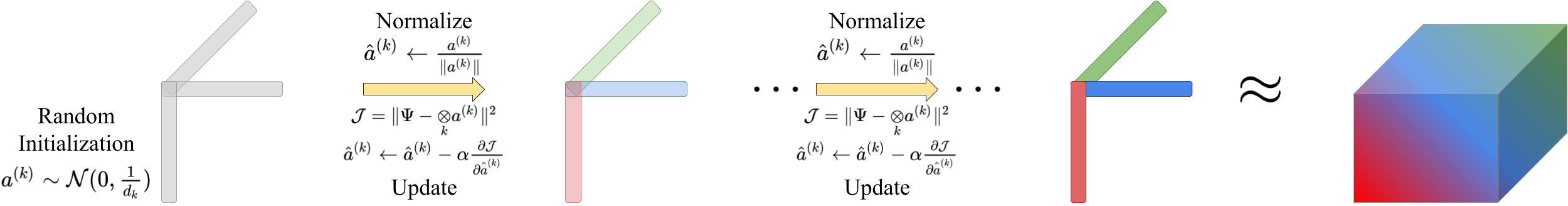
Figure 1: Illustration of our NGD algorithm for finding a rank $1$ approximation of a tensor $\Psi$.

3.4 Symmetrized gradient descent

Analogous to the power iterations method [Evn21], we develop a symmetrized version of NGD, the symmetrized gradient descent (SGD) algorithm, to approximate symmetric tensors. It optimizes the Euclidean norm loss objective over $R$ symmetric product states and hence estimates $R$ cores, with each $\hat{a}_{r}\in\mathbb{R}^{d}$ or $\mathbb{C}^{d}\;\forall\;r\in 1,2,\ldots,R$.

$$\hat{\phi}=\sum_{r=1}^{R}\hat{a}_{r}^{\otimes n}$$ (10)

Algorithm 2 Symmetrized Gradient Descent to approximate symmetrized $\Psi$ with $\phi\in\operatorname{PRO}$

0:  $\phi\in\operatorname{PRO}$

0:  $\|\phi\|$ = 1

1:  Initialize: $a_{r}\sim\mathcal{N}(0,\frac{1}{d_{k}})\;\forall\;r\in 1,2,\cdots,R$

2:  if $\Psi$ is complex then

3:     $a^{\prime(k)}_{r}\sim\mathcal{N}(0,\frac{1}{d_{k}})\;\forall\;r\in 1,2,\ldots,R,\;\forall\;k\in 1,2,\ldots,n$

4:     $a^{(k)}_{r}\leftarrow(a^{(k)}_{r}+a^{\prime(k)}_{r})/\sqrt{2}$

5:  end if

6:  $t=0$

7:  for $t<\texttt{max\_epochs}$ do

8:     $\hat{a}_{r}\leftarrow\frac{a_{r}}{\|a_{r}\|}\;\forall\;r\in 1,2,\ldots,R$

9:     $\hat{\phi}\leftarrow\sum_{r=1}^{R}\hat{a}_{r}^{\otimes n}$

10:     $\mathcal{J}\leftarrow\mathcal{L}(\Psi,\hat{\phi})$

11:     $\hat{a}_{r}\leftarrow\hat{a}_{r}-\alpha\frac{\partial\mathcal{J}}{\partial\hat{a}_{r}}\;\forall\;r\in 1,2,\ldots,R$

12:     $t\leftarrow t+1$

13:  end for

4 Benchmarking the algorithms on random tensors

In this section, we test how the algorithms presented in Section 3 perform. We are going to focus on tensors of order $2$ and $3$. The injective norm of order $2$ tensors is precisely the operator norm of the corresponding matrix, i.e. the largest singular value of the operator. This allows us to compare the performance of the algorithms to their established counterparts from linear algebra. The case of order $3$ tensors is fundamentally much more complex [HL13]. Computing the injective norm of order $3$ tensors is already an NP-hard problem [HL13, Theorem 1.10]. We investigate random tensors with large local dimension $d$, in the spirit of Random Matrix Theory, where most analytical results are obtained in the limit of large matrix dimension. For tensors of order $3$ or more, the only analytical results for the injective norm of random Gaussian tensors are obtained in the asymptotic regime $d\to\infty$, for real symmetric Gaussian tensors [ABAČ13, PWB20]. Although the algorithms we present work for general tensors of any order, we focus here on order $3$ tensors for two reasons: the computational overheads (time and space complexity) grow exponentially with the order, while order $3$ tensors encompass all the theoretical and computational challenges encountered while dealing with higher order tensors.

4.1 Random model used for benchmarking

We estimate the injective norm of a certain class of random tensors in $(\mathbb{R}^{d})^{\otimes n}$, namely real Gaussian tensors and their symmetrized counterparts. Indeed, there are known exact results from previous works for the injective norm of symmetrized real Gaussian tensors [ABAČ13, PWB20]. So we can compare the numerical values obtained by our algorithms to these analytical ones. The choice that we will make for the variance of the entries may seem a bit unintuitive. However, as we will see later, it is a normalization that guarantees that the injective norm of the tensor converges to a finite non-zero value as $d$ grows.

4.1.1 Real Gaussian tensors

A real Gaussian tensor $X\in\left(\mathbb{R}^{d}\right)^{\otimes n}$ is formed by sampling each of its entries from $\mathcal{N}\left(0,\frac{2}{d}\right)$.

$$X_{i_{1},i_{2},\ldots,i_{n}}\sim\mathcal{N}\left(0,\frac{2}{d}\right)\;\forall\;i_{j}\in\{1,2,\ldots,d\}\;\forall\;j\in\{1,2,\ldots,n\}$$ (11)

The expected value of the squared Euclidean norm of such tensor is simply the dimension of $(\mathbb{R}^{d})^{\otimes n}$, multiplied by the variance factor $\frac{2}{d}$, i.e. $\frac{2}{d}\times d^{n}=2d^{n-1}$. The expected Euclidean norm of such tensor is thus equivalent to $\sqrt{2d^{n-1}}$ for large $d$.

4.1.2 Symmetrized Gaussian tensors

A (fully) symmetrized real Gaussian tensor $X_{s}\in\left(\mathbb{R}^{d}\right)^{\otimes n}$ can be formed by projecting a real Gaussian tensor $X\in\left(\mathbb{R}^{d}\right)^{\otimes n}$ onto the symmetric subspace of $\ \left(\mathbb{R}^{d}\right)^{\otimes n}$. Concretely, we do the following.

1. Form an auxiliary Gaussian tensor $X\in\left(\mathbb{R}^{d}\right)^{\otimes n}$ with each entry sampled from $\mathcal{N}\left(0,\frac{2}{d}\right)$.

   $$X_{i_{1},i_{2},\ldots,i_{n}}\sim\mathcal{N}\left(0,\frac{2}{d}\right)\;\forall\;i_{j}\in\{1,2,\ldots,d\}\;\forall\;j\in\{1,2,\ldots,n\}$$ (12)

2. Average over each possible permutation of the auxiliary tensor’s axes.

   $$X_{s_{i_{1},i_{2},\ldots,i_{n}}}=\frac{1}{n!}\sum_{\sigma\in S_{n}}X_{i_{\sigma(1)},i_{\sigma(2)},\ldots,i_{\sigma(n)}}\;\forall\;i_{j}\in\{1,2,\ldots,d\}\;\forall\;j\in\{1,2,\ldots,n\},$$ (13)

   where $S_{n}$ is the permutation group of $n$ elements.

The symmetrized tensor $X_{s}$ has its entries sampled from $\mathcal{N}\big{(}0,\frac{2}{dn!}\big{)}$ for locations with no repeated indices. The expected value of the squared Euclidean norm of such a tensor is simply the dimension of the symmetric subspace of $(\mathbb{R}^{d})^{\otimes n}$, multiplied by the variance factor $\frac{2}{d}$, i.e. $\frac{2}{d}\times\binom{d+n-1}{n}=2\frac{(d+n-1)\times\cdots\times(d+1)}{n!}$. The expected Euclidean norm of such tensor is thus equivalent to $\sqrt{\frac{2}{n!}d^{n-1}}$ for large $d$.

Let us point out that the factor $2$ in the variance of the normal distribution in Equations (11) and (12) is not completely arbitrary. It is indeed the normalization that is standard in the symmetric case, since in the case $n=2$, where the tensor $X_{s}$ can be identified with a symmetric matrix, it guarantees that the off-diagonal terms have variance $1/d$ while the diagonal ones have variance $2/d$. We, therefore, use this normalization as well so that the numerical value we obtain for the injective norm of $X_{s}$ can be directly compared to analytical results in the literature, such as those presented in [PWB20]. We then use this same normalization in the non-symmetric case just to simplify the analysis: that way the symmetrized tensor has an expected Euclidean norm which is asymptotically (as $d\rightarrow\infty$) scaled by a factor $\frac{1}{\sqrt{n!}}$ as compared to the non-symmetrized tensor.

4.2 Results

Analytical results for the injective norms of random tensors are quite limited. It is known that, as $d\rightarrow\infty$, the injective norm of an order $n$ symmetric real Gaussian tensor converges to some value $\eta_{n}$, which is defined as the unique solution to some explicit equation [ABAČ13, PWB20]. This quantity $\eta_{n}$ can thus be estimated numerically for fixed values of $n$, and its asymptotic behaviour as $n\rightarrow\infty$ can be identified to be equivalent to $\sqrt{\log n}$. However, the approach used to obtain this precise asymptotic estimate unfortunately breaks down for non-symmetrized real Gaussian tensors. In this case, only estimates on the order of magnitude of the injective norm can be derived. They tell us that, as $d\rightarrow\infty$, the injective norm of an order $n$ (non-symmetrized) real Gaussian tensor converges to some $n$-dependent value which scales as $\sqrt{n\log n}$ for $n\rightarrow\infty$. A proof that this injective norm is asymptotically $O(\sqrt{n\log n})$ can be found in [TS14], while corresponding $O(\sqrt{n\log n})$ and $\Omega(\sqrt{n\log n})$ asymptotic estimates are established in the work in progress [LN].

We first benchmark the performance of all the algorithms on symmetrized real Gaussian tensors because as explained above, those are the only random tensors for which the asymptotic limit of their injective norm is known. We compare the performance of ALS and NGD along with their symmetrized counterparts, PIM and SGD. For symmetrized Gaussian tensors, the asymptotic values of the injective norm are $2$ and $2.343334$ for order $2$ and order $3$ respectively, referred from [PWB20]. As shown in Figure 2, for order $2$ tensors, all algorithms perform equally and converge within $2.5\%$ of the analytical upper bound. However, for order $3$ tensors, NGD and SGD show negligible disparity in performance while greatly outperforming ALS and PIM.

Further, we estimate and compare the expected values of the injective norm of non-symmetrized real Gaussian tensors using both ALS and NGD. We know that for order $2$, the injective norm converges to $2\sqrt{2}$ as $d\rightarrow\infty$. Both algorithms perform at par on order $2$ tensors. Although the analytical value for order $3$ tensors is unknown, we know that all numerical algorithms estimate a lower bound on the true value of the injective norm. It is thus clear that NGD outperforms ALS by a substantial margin as shown in Figure 3.

We suspect that ALS and PIM perform sub-optimally since the Euclidean norm of the candidate $\|\phi\|$ depends on that of the original tensor $\|\Psi\|$. Upon normalizing the ALS result post-convergence, the dependence of $\|\phi\|$ on $\|\Psi\|$ induces a sub-optimal lower bound on the injective norm as $\|\Psi\|$ grows with $d$. Our proposed NGD and SGD algorithms mitigate this problem by eradicating the dependence of $\|\phi\|$ on $\|\Psi\|$ and by restricting $\phi$ to be a product state through normalization on each step of the iterative optimization process. Further, our proposed NGD algorithm adapts to symmetrization and performs best on both symmetrized and non-symmetrized Gaussian tensors.

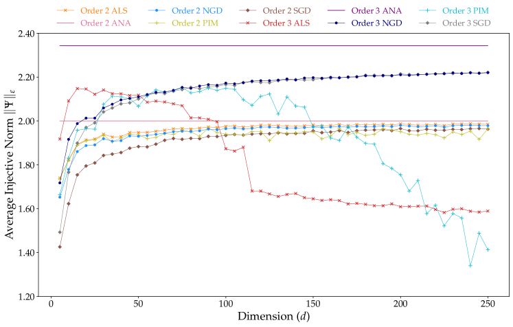
Figure 2: The average injective norm of symmetrized real Gaussian tensors approximated using the ALS, PIM, NGD and SGD algorithms. All the algorithms perform equally well on order $2$ tensors. NGD and SGD perform substantially better than ALS and PIM on order $3$ tensors. The analytical bounds are labeled “ANA”.

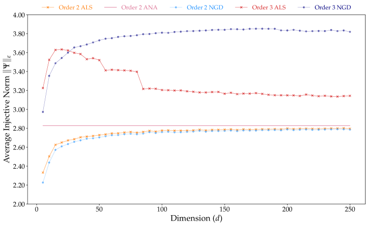
Figure 3: The average injective norm of non-symmetrized real Gaussian tensors approximated using the ALS and NGD algorithms. Both algorithms perform equally well on order $2$ tensors. NGD performs substantially better than ALS on order $3$ tensors since both algorithms estimate a lower bound.

4.3 The effect of normalization

As mentioned in Sections 3.1 and 3.2, the norm of the approximation $\|\phi\|$ is affected by the norm of the original tensor $\|\Psi\|$ when using the ALS and PIM algorithms. Hence, we also benchmark the performance of all the algorithms on normalized initial tensors $\hat{\Psi}=\Psi/\|\Psi\|$. In this case, all algorithms perform at par on both symmetrized and non-symmetrized real Gaussian tensors. It can, however, be an issue to be forced to work with normalized inputs. Indeed, in situations such as the ones we are considering here, where the injective norm is much smaller than the Euclidean norm, if the input tensor is normalized, then the output (normalized injective norm) goes to $0$ as $d\rightarrow\infty$. To avoid numerical instability and to be able to analyze the results better, it is preferable in such cases to have an algorithm where the input can be scaled so that the output goes to a finite, non-zero, asymptotic value.

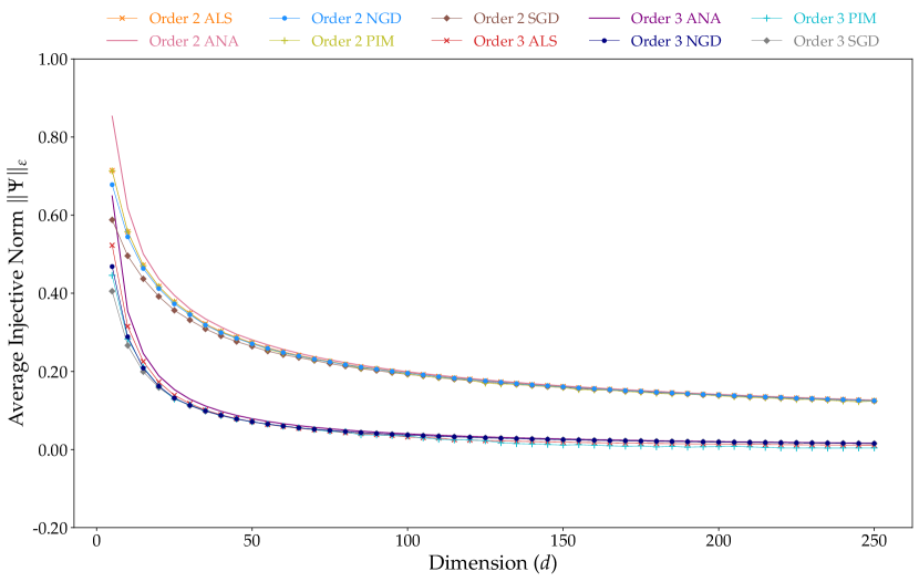
(a) Normalized symmetrized real Gaussian tensors.

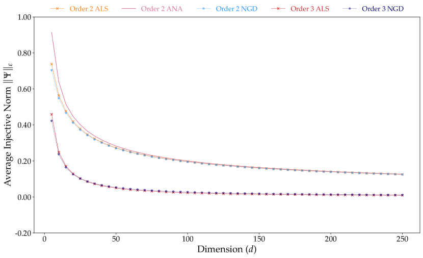
(b) Normalized non-symmetrized real Gaussian tensors.

Figure 4: All algorithms perform equally well on inputs that are normalized real Gaussian tensors, either symmetrized or non-symmetrized. However, it is preferable in this case to work with non-normalized tensors because otherwise the injective norm goes to $0$ as $d\to\infty$.

Having established that NGD allows for inputs that are non-normalized (while performing as well as ALS on normalized ones) or non-symmetric (while performing as well as SGD on symmetric ones), it is the one we will systematically use in the sequel. In particular, we will employ it to estimate the injective norm of complex Gaussian tensors (in Section 5) and Gaussian matrix product states (in Section 6).

On the other hand, we present in Appendix A results that confirm that both the ALS and NGD algorithms perform well on normalized tensors. More precisely, we test ALS and NGD on some classes of deterministic multipartite pure states (both sparse and dense) with known values of GME, and we observe equally good performance from both algorithms. In fact, let us point out that we have not found any example of a tensor (either sparse or dense, either deterministic or random, either real or complex) for which our NGD algorithm fails to approximate its injective norm with good accuracy.

4.4 Numerical function estimators

As mentioned in Section 4.2, the asymptotic value (as $d\rightarrow\infty$) of the injective norm is known exactly only for symmetrized real Gaussian tensors, and only its scaling in $n$ is known for non-symmetrized real Gaussian tensors. Further, even for symmetrized real Gaussian tensors, an exact analytical function for finite $d$ is still unknown. In what follows, we provide numerical estimates of two kinds: (a) for all cases (symmetrized and non-symmetrized, order $2$ and $3$), we estimate the asymptotes, (b) for the cases were the asymptote is known (symmetrized order $2$ and $3$, non-symmetrized order $2$), we estimate the leading correction term.

For estimating the asymptotes, we fit a geometric series $(C_{0}r^{k})_{k\in\mathbb{N}}$ with $|r|<1$ on the first differences of our data points. This choice is motivated by the fact that, with the normalization that we choose, as $d\rightarrow\infty$, the injective norm converges to a fixed constant value and the difference between successive terms vanishes. The infinite sum of the series then gives us the difference between the first data point and the asymptote as $\frac{C_{0}}{1-|r|}$. We apply this method to all four cases, order $2$ and $3$, symmetrized and non-symmetrized real Gaussian tensors. In the three cases where the analytical value is known, we observe that our obtained numerical estimates match closely with the analytical values [PWB20] as shown in Table 1.

Order	Symmetry	Field	Estimated asymptote $C_{0}$	Analytical asymptote	% Error
2	Symmetrized	$\mathbb{R}$	$1.978929$	$2.000000$	$1.053563$
	Non-symmetrized	$\mathbb{R}$	$2.794735$	$2.828427$	$1.191190$
3	Symmetrized	$\mathbb{R}$	$2.248792$	$2.343334$	$4.034520$
	Non-symmetrized	$\mathbb{R}$	$3.949725$	-	-

Table 1: Estimates for the asymptotic value of the injective norm of real Gaussian tensors.

Further, we estimate the leading correction term in the three cases where the asymptote is analytically known. To do this, we fit function estimators of the form $C_{0}+C_{1}d^{\alpha}$, where $C_{0}$ is a fixed constant (the known analytical asymptote), whereas $C_{1}$ and $\alpha$ are estimated by minimizing the squared error.

In the case of order $2$ symmetrized real Gaussian tensors, the theoretical value for $\alpha$ is conjectured to be $-2/3$, due to the following known fact: Let $G$ be a $d\times d$ GOE matrix, normalized so that its off-diagonal entries have variance $\frac{1}{d}$ and its diagonal ones have variance $\frac{2}{d}$. Note that $G$ is the same as a symmetric real Gaussian tensor of order $2$, as defined in Section 4.1.2, viewed as a matrix rather than a vector. In this matrix picture, the equivalent of the injective norm is simply the largest eigenvalue. Now, we know (see e.g. [AS17, Proposition 6.25]) that for such random matrix $G$, for any $0<\delta<1$,

$$\mathbb{P}\left(\lambda_{max}(G)>2+\delta\right)\leq e^{-cd\delta^{3/2}}\text{ and }\mathbb{P}\left(\lambda_{max}(G)<2-\delta\right)\leq e^{-c^{\prime}d^{2}\delta^{3}}.$$

Both deviation probabilities are non-vanishing for $\delta\simeq d^{-2/3}$. So, supposing they are sharp, we expect that, for finite but large $d$, a good estimator for the behaviour of $\lambda_{max}(G)$ would be of the form $2+Cd^{-2/3}$. We observe that the numerical values we obtain for $\alpha$ in the order $2$ case (in fact for both symmetrized and non-symmetrized Gaussian tensors) match with this conjectured value of $-2/3$, as shown in Table 2.

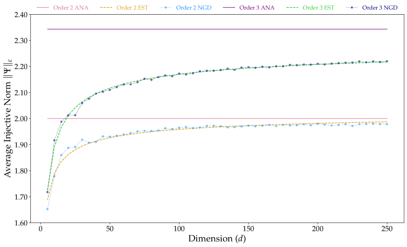
(a) Symmetrized real Gaussian tensors.

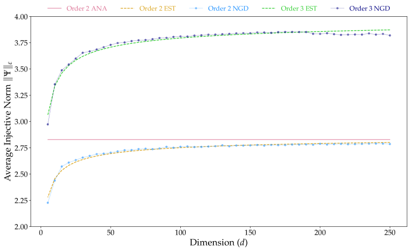
(b) Non-symmetrized real Gaussian tensors.

Figure 5: We fit functions of the form $C_{0}+C_{1}d^{\alpha}$ on the data points obtained using the NGD algorithm for symmetrized and non-symmetrized real Gaussian tensors of order $2$ and $3$. The asymptotic constant $C_{0}$ matches the analytical value (known for all order $2$ tensors and only for symmetrized real Gaussian tensors of order $3$) with less than $5\%$ error as shown in Table 1.

Order	Symmetry	Field	Analytical asymptote $C_{0}$	Coefficient $C_{1}$	Power $\alpha$
2	Symmetrized	$\mathbb{R}$	$2.000000$	$-0.99787802$	$-0.69016213$
	Non-symmetrized	$\mathbb{R}$	$2.828427$	$-1.61362670$	$-0.63377984$
3	Symmetrized	$\mathbb{R}$	$2.343334$	$-1.16629229$	$-0.41246088$
	Non-symmetrized	$\mathbb{R}$	-	-	-

Table 2: Estimates for the leading correction term in the cases where the asymptotic values are analytically known. These values are obtained by fitting curves of the form $C_{0}+C_{1}d^{\alpha}$, where $C_{0}$ is fixed (to the known asymptotic value) while $C_{1}$ and $\alpha$ are estimated by minimizing the squared error.

5 Complex Gaussian tensors

In this section, we look at random complex Gaussian tensors in $\left(\mathbb{C}^{d}\right)^{\otimes n}$, starting with a brief description of how we construct these tensors. Having established that our proposed NGD algorithm performs better than the others in all cases, we employ it to obtain lower bounds on the injective norm of complex Gaussian tensors and their symmetrized counterparts. In the complex setting, contrary to the real one, no analytical results are known for the asymptotic value of these norms (even in the symmetric case). Note that a complex Gaussian tensor, after dividing by its Euclidean norm, has the same distribution as a uniform complex unit tensor. Hence, computing the injective norm of a (normalized) complex Gaussian tensor (either symmetrized or not) is equivalent to computing the amount of entanglement in a uniformly distributed multipartite pure state (with or without the constraint of being permutation-invariant). The numerical results that we obtain are thus the first precise estimates on the amount of entanglement in such random multipartite pure states. They furthermore allow us to quantitatively study the effect of symmetrization on the entanglement present in generic multipartite pure states.

5.1 Construction

We construct a complex Gaussian tensor $X\in\left(\mathbb{C}^{d}\right)^{\otimes n}$ by sampling the real and imaginary parts of each of its entries from $\mathcal{N}\big{(}0,\frac{2}{d}\big{)}$. Further, we normalize each entry by a factor of $\sqrt{2}$ to maintain the expected value of the Euclidean norm of the complex Gaussian tensors the same as that of real Gaussian tensors with the same local dimension $d$ and number of tensor factors $n$. Similarly, we construct a symmetrized complex Gaussian tensor $X_{s}\in\left(\mathbb{C}^{d}\right)^{\otimes n}$ by first sampling the real and imaginary parts of each entry of the complex Gaussian tensor $X\in\left(\mathbb{C}^{d}\right)^{\otimes n}$ from $\mathcal{N}\big{(}0,\frac{2}{d}\big{)}$ and normalizing by a factor of $\sqrt{2}$ before projecting it onto the symmetric subspace of $\left(\mathbb{C}^{d}\right)^{\otimes n}$.

5.2 Estimating the injective norm

We estimate the injective norm of complex Gaussian tensors and their symmetrized counterparts using the NGD algorithm. The asymptotic value for order $2$ tensors is known to be $2\sqrt{2}$ and $2$ as $d\rightarrow\infty$ for the non-symmetrized and symmetrized models, respectively. As mentioned in Section 4.2, for higher order tensors, no exact asymptotic estimate is known. The only thing that can be shown is that, with the normalization that we use for the variance, the injective norm converges to an $n$-dependent limit as $d\rightarrow\infty$, and as $n\rightarrow\infty$ the limit scales as $\sqrt{n\log n}$ in the non-symmetrized case and as $\sqrt{\log n}$ in the symmetrized case. This asymptotic scaling is exactly the same as for real Gaussian tensors in both the symmetrized and the non-symmetrized cases. It is explained how to derive such estimates on the order of magnitude of these norms in [AS17]. The precise computations are done in the work in progress [LN]. Let us just point out that it is not clear at all whether the techniques used in [ABAČ13] to get an exact asymptotic estimate for the injective norm of a real symmetric Gaussian tensor could be applied to treat at least the case of symmetric complex Gaussian tensors.

The numerical results that we obtain for the injective norm of order $2$ and order $3$ complex Gaussian tensors are shown in Figures 6(a) (non-symmetrized case) and 7(a) (symmetrized case). In the complex case, we estimate the asymptotic value and the leading correction term using the same two-step strategy as in the real case, and function estimators of the same form.

Let us point out that, for order $2$ Gaussian tensors, the analytical asymptotic values are the same for real and complex symmetrized tensors on the one hand, and for real and complex non-symmetrized tensors on the other hand. Numerically, we observe that this seems to be the case also for order $3$ Gaussian tensors. Motivated by this evidence, we conjecture that the asymptotic limits of the injective norms for corresponding (same order and symmetry) real and complex Gaussian tensors are identical. All numerical estimates for the asymptotic values are presented in Table 3.

Further, we estimate the leading correction term by fitting function estimators of the form $C_{0}+C_{1}d^{\alpha}$, like in the real case. Building upon our conjecture, we use the same value for $C_{0}$ in the order $3$ symmetrized complex Gaussian case as in the real one, and observe that the correction coefficient and power match closely with those in the real case as shown in Tables 2 and 4.

Order	Symmetry	Field	Estimated asymptote $C_{0}$	Analytical asymptote	% Error
2	Symmetrized	$\mathbb{C}$	$2.092316$	$2.000000$	$4.6158$
	Non-symmetrized	$\mathbb{C}$	$2.946784$	$2.828427$	$4.1846$
3	Symmetrized	$\mathbb{C}$	$2.356248$	$-$	$-$
	Non-symmetrized	$\mathbb{C}$	$4.143529$	$-$	$-$

Table 3: Estimates for the asymptotes for complex Gaussian tensors. Unlike in the real case, in the complex case we do not know the analytical value for the order 3 symmetrized Gaussian tensors. However, we observe that the value is quite close to the real case and hence we conjecture that they are indeed the same value.

Order	Symmetry	Field	Analytical asymptote $C_{0}$	Coefficient $C_{1}$	Power $\alpha$
2	Symmetrized	$\mathbb{C}$	$2.000000$	$-0.83908193$	$-0.63376019$
	Non-symmetrized	$\mathbb{C}$	$2.828427$	$-1.68679358$	$-0.63961335$
3	Symmetrized	$\mathbb{C}$	$2.343334$	$-0.90616281$	$-0.39636923$
	Non-symmetrized	$\mathbb{C}$	-	-	-

Table 4: Estimates for the leading correction term in the cases where the asymptotic values are analytically known or conjectured. The leading correction coefficient and power are obtained by fitting curves of the form $C_{0}+C_{1}d^{\alpha}$, where $C_{0}$ is fixed (to the known or conjectured asymptotic value), while $C_{1}$ and $\alpha$ are estimated by minimizing the squared error.

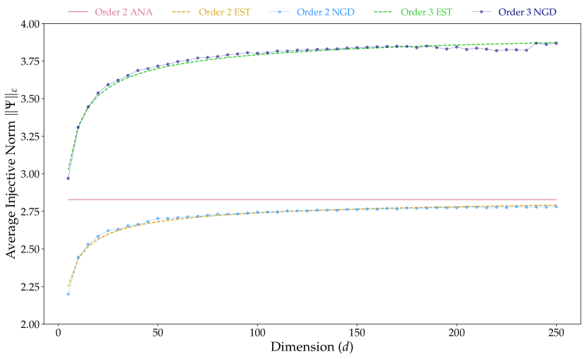
(a) Non-symmetrized complex Gaussian tensors.

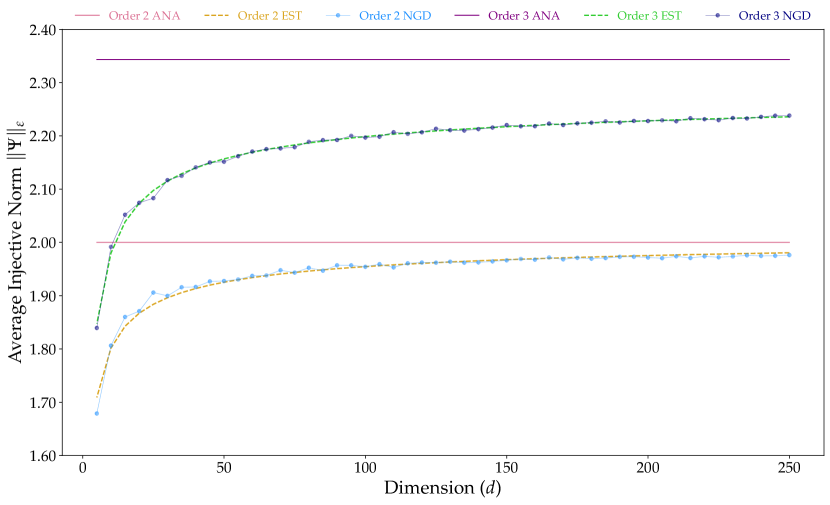
(a) Symmetrized complex Gaussian tensors.

Figure 7: We approximate the average value of the injective norm of both symmetrized and non-symmetrized complex Gaussian tensors using the NGD algorithm. Further, we fit function estimators of the form $C_{0}+C_{1}d^{\alpha}$ on these data points. The estimated values of $C_{0}$, resp., $C_{1}$ and $\alpha$, are given in Table 3, resp., Table 4.

5.3 The effect of symmetrization on entanglement

In this section we want to understand how symmetrizing a multipartite pure state affects the amount of entanglement present in it. More precisely, given a multipartite pure state $\hat{\Psi}\in(\mathbb{C}^{d})^{\otimes n}$, we define its symmetrization

$$\Psi_{S}:=\frac{1}{n!}\sum_{\sigma\in S_{n}}\sigma.\hat{\Psi},$$

where $\sigma\in S_{n}$ acts on $\hat{\Psi}$ by permuting the tensor factors, and the corresponding symmetric multipartite pure state $\hat{\Psi}_{S}=\frac{\Psi_{S}}{\|\Psi_{S}\|}$. ($\Psi_{S}$ being the projection of $\hat{\Psi}$ onto the symmetric subspace of $(\mathbb{C}^{d})^{\otimes n}$, it is in general subnormalized.) We would then like to compare the entanglement of $\hat{\Psi}$ and $\hat{\Psi}_{S}$. Intuitively, one would think that $\hat{\Psi}_{S}$ is generically less entangled than $\hat{\Psi}$, i.e.

$$\|\hat{\Psi}_{S}\|_{\varepsilon}\geq\|\hat{\Psi}\|_{\varepsilon}.$$ (14)

Note that Equation (14) does not hold true for all multipartite pure states. For instance, $\hat{\Psi}=|12\rangle\in(\mathbb{C}^{2})^{\otimes 2}$ is separable, while its normalized symmetrization $\hat{\Psi}_{S}=\frac{1}{\sqrt{2}}(|12\rangle+|21\rangle)$ is maximally entangled. However, we expect that, for large $d$, multipartite pure states in $(\mathbb{C}^{d})^{\otimes n}$ typically satisfy Equation (14).

We now employ our NGD algorithm to quantitatively study the effect of symmetrization on the amount of entanglement present in random multipartite pure quantum states with a Gaussian distribution. We do so by computing the expected normalized injective norm of both symmetrized and non-symmetrized complex Gaussian tensors. Indeed, we recall that $\|\hat{\Psi}\|_{\varepsilon}=2^{-\operatorname{GME}(\Psi)/2}$ is equal to $1$ only for product states $\hat{\Psi}$ and approaches $0$ as $d$ grows for highly entangled states.

Figures 8(a) and 9(a) show that entanglement increases with the dimension $d$ of the tensor, regardless of symmetry. Also, the value of $\|\hat{\Psi}\|_{\varepsilon}$ and $\operatorname{GME}(\Psi)$ for order $2$ tensors remains the same, regardless of symmetry, owing to the choice of normalization factor described in Section 4.1.2. However, for order $3$ tensors, symmetrization decreases the amount of entanglement in the tensor and increases the value of $\|\hat{\Psi}\|_{\varepsilon}$. The plots in Figure 10(a) illustrate that for order $3$ tensors, symmetrization results in a larger value of $\|\hat{\Psi}\|_{\varepsilon}$, i.e. symmetrized tensors are less entangled than their non-symmetrized counterparts. Hence, we can conclude that projecting a random Gaussian tensor onto the symmetric subspace of $\left(\mathbb{C}^{d}\right)^{\otimes n}$ results in a less entangled tensor.

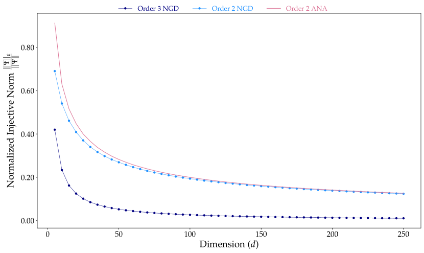
(a) Non-symmetrized complex Gaussian tensors.

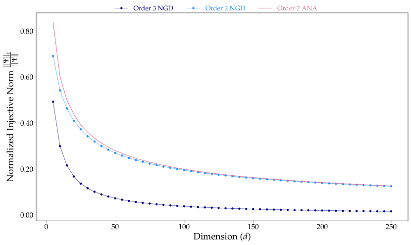
(a) Symmetrized complex Gaussian tensors.

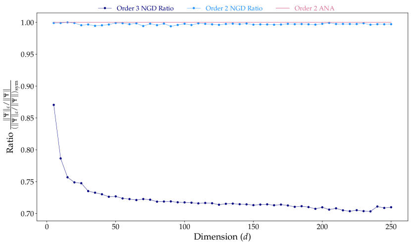
(a) The ratio of the normalized injective norm of non-symmetrized complex Gaussian tensors to that of their symmetrized counterparts.

Figure 10: Entanglement in both symmetrized and non-symmetrized complex Gaussian tensors increases with increasing $d$. The value of $\|\Psi\|_{\varepsilon}$ for symmetrized Gaussian tensors is greater than (for order $3$ and above) or equal to (for order $2$) that for non-symmetrized Gaussian tensors of the same order and dimension. This indicates that symmetrizing a random Gaussian tensor reduces entanglement.

6 Random matrix product states

In this section, we look at a model of random multipartite pure quantum states which might be more interesting than uniformly distributed states from a physical point of view, namely random matrix product states (MPS). MPS are used extensively in quantum condensed matter physics as an Ansatz for the ground states of gapped local Hamiltonians on 1D systems [Has06, LVV15]. Studying typical properties of MPS is a research direction that has recently attracted a lot of attention, as it means studying typical properties of physically relevant many-body quantum systems. The quantities that have been looked at up to now include the generic amount of entanglement between a bipartition of the sites [GdOZ10, CGGPG13, GGJN18, HBRE21] and the generic amount of correlations between two distant sites [LPG22]. Similar to the case of complex Gaussian random tensors, we go beyond the bipartite paradigm and obtain here the first estimates on the genuinely multipartite entanglement of random MPS.

6.1 Gaussian matrix product states

To construct a random MPS $X\in\mathbb{C}^{d_{1}}\otimes\mathbb{C}^{d_{2}}\otimes\cdots\otimes\mathbb{C}^{d_{n}}$ with periodic boundary conditions, we start by sampling $n$ local tensors $A^{(k)}\in\mathbb{C}^{q_{k}}\otimes\mathbb{C}^{d}\otimes\mathbb{C}^{q_{k+1}}$, for $k\in\{1,2,\ldots,n\}$, with $q_{n+1}=q_{1}$. The local dimensions $d_{k}$ and $q_{k}$ are called the physical and bond dimensions, respectively.

$$A^{(k)}_{i_{1},s,i_{2}}\sim\mathcal{N}\left(0,\frac{2}{d_{k}\sqrt{q_{k}q_{k+1}}}\right)\;\forall\;i_{1}\in\{1,2,\ldots,q_{k}\},s\in\{1,2,\ldots,d_{k}\},i_{2}\in\{1,2,\ldots,q_{k+1}\}$$ (15)

We sample the real and imaginary parts of each entry of the local tensors as described in Equation (15), and normalize by a factor of $\sqrt{2}$. We then contract the local tensors over the internal bond dimensions and identify the last index with the first index.

$$X_{s_{1},s_{2},\cdots,s_{n}}=\sum_{i_{1},i_{2},\cdots,i_{n}}A^{(1)}_{i_{1}s_{1}i_{2}}A^{(2)}_{i_{2}s_{2}i_{3}}\cdots A^{(n)}_{i_{n}s_{n}i_{1}}$$ (16)

When the local tensors $A^{(k)}$ are sampled as described in Equation (15), independently from one another, the expected value of the squared Euclidean norm of the corresponding Gaussian MPS is simply $d_{1}\times\cdots\times d_{n}\times q_{1}\times\cdots\times q_{n}\times\frac{2}{d_{1}\sqrt{q_{1}q_{2}}}\times\cdots\times\frac{2}{d_{n}\sqrt{q_{n}q_{1}}}=2^{n}$.

Translation-invariance can be incorporated in this model of random MPS by repeating the same local tensor $A^{(k)}$ on all sites, with all $q_{k}=q$ and $d_{k}=d$. In this case, the expected value of the squared Euclidean norm of the corresponding translation-invariant Gaussian MPS is $2^{n}+o(1)$ as $d,q\rightarrow\infty$.

In what follows, we will focus on presenting estimates on the normalized injective norm in the following cases: random MPS with periodic boundary conditions, constructed from either independent or repeated complex Gaussian tensors on each site. We will present the results obtained for such random tensors of order $3$. Indeed, as already explained, computing the injective norm of order $2$ tensors is not particularly challenging, and all the theoretical and computational challenges encountered for higher order tensors are already encompassed in the order $3$ case.

An important observation is that the normalized injective norm of a Gaussian MPS, unlike the one of a Gaussian tensor, does not necessarily go to $0$ as $d\to\infty$. It indeed depends on both parameters $d$ and $q$, in a way that is quite complicated to grasp. The goal of the subsequent analysis is to try and understand better this dependence on $d$ and $q$, in different asymptotic regimes.

In the work in progress [LN], it is proven that the injective norm of a Gaussian MPS in $(\mathbb{C}^{d})^{\otimes n}$ with bond dimension $q$ (either translation-invariant or not) is of order $\max\left(\frac{1}{\sqrt{d^{n-1}}},\frac{1}{\sqrt{q^{n-1}}}\right)$, as $d,q\rightarrow\infty$ (up to a potential $n$-dependent multiplicative factor). It is not clear how this joint asymptotic scaling in $d$ and $q$ could be numerically confirmed in a reliable way. It would indeed require to fit the asymptotic injective norm as $d$ and $q=q(d)$ grow at various relative speeds. Instead, we focus in what follows on the two extreme cases where either $q$ is fixed and $d$ grows or $d$ is fixed and $q$ grows.

6.2 Scaling with physical dimension for fixed bond dimension

Similar to the Gaussian tensors, we estimate the numerical lower bounds on the asymptotic injective norm of order $3$ Gaussian MPS with a fixed bond dimension $q$, as $d\rightarrow\infty$. The results are presented in Figures 11(a) (for independent local tensors) and 12(a) (for repeated local tensors). We use the same approach of fitting a geometric series of the form $(C_{0}r^{k})_{k\in\mathbb{N}}$ on the first differences of the data points. We report the values of the asymptotes in Table 5.

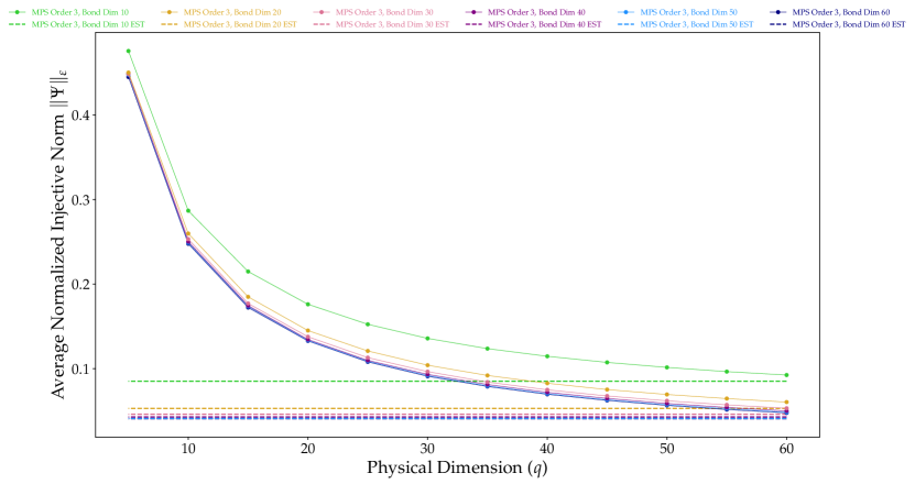
(a) Gaussian MPS without translation-invariance.

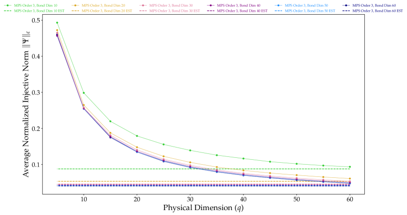
(a) Gaussian MPS with translation-invariance.

Figure 12: For both cases (with and without translation-invariance), for a fixed $q$, as $d$ increases, the value of the normalized injective norm decreases, indicating that entanglement increases with $d$. Further, we fit a geometric series of the form $(C_{0}r^{k})_{k\in\mathbb{N}}$ on the first differences of the data points obtained using the NGD algorithm. The estimated values of the asymptotes are given in Table 5.

Translation Invariance	Bond Dimension	Estimated asymptote
With	10	$0.087853$
	20	$0.053398$
	30	$0.045909$
	40	$0.043447$
	50	$0.041846$
	60	$0.040545$
Without	10	$0.085244$
	20	$0.053005$
	30	$0.046096$
	40	$0.042909$
	50	$0.041235$
	60	$0.040860$

Table 5: Estimates for the asymptotes for fixed bond dimensions obtained by fitting a geometric series of the form $(C_{0}r^{k})_{k\in\mathbb{N}}$ on the first differences of the data points obtained using our NGD algorithm for Gaussian MPS with periodic boundary conditions, with and without translation-invariance.

6.3 Scaling with bond dimension for fixed physical dimension

Similar to the case with a fixed bond dimension, we also estimate the asymptotes for fixed physical dimensions by fitting a geometric series of the form $(C_{0}r^{k})_{k\in\mathbb{N}}$ on the first differences of the data points obtained using our NGD algorithm for Gaussian MPS with periodic boundary conditions, with and without translation-invariance. We present these estimates in Table 6.

We are now interested in comparing the amount of entanglement in a Gaussian MPS and its corresponding Gaussian tensor. We conjecture that, if the physical dimension $d$ is fixed, then as the bond dimension $q$ increases, the value of the normalized injective norm of a Gaussian MPS in $\left(\mathbb{C}^{d}\right)^{\otimes n}$ converges to that of a corresponding Gaussian tensor in $\left(\mathbb{C}^{d}\right)^{\otimes n}$. The latter is either a non-symmetrized Gaussian tensor, in the case where the MPS has independent local tensors, or a cyclically symmetrized Gaussian tensor (see precise definition below), in the case where the MPS has repeated local tensors. In what follows, we explain our choice of correspondence between MPS and Gaussian tensors along with numerical evidence to support our claim.

6.3.1 Comparing non-translation-invariant MPS to non-symmetrized Gaussian tensors

We compare MPS in $\left(\mathbb{C}^{d}\right)^{\otimes n}$ with $n$ sites, each having a physical dimension $d$ and bond dimension $q$, with periodic boundary conditions and independent Gaussian local tensors (i.e. without translation-invariance) to non-symmetrized Gaussian tensors in $\left(\mathbb{C}^{d}\right)^{\otimes n}$. Since all entries for each local tensor in such an MPS are drawn independently and identically from the same distribution, and all local tensors contribute equally to the construction (periodic boundary conditions), we consider this case to be the closest to a non-symmetrized Gaussian tensor.

6.3.2 Comparing translation-invariant MPS to cyclically symmetrized Gaussian tensors

Further, we compare MPS in $\left(\mathbb{C}^{d}\right)^{\otimes n}$ with $n$ sites, each having a physical dimension $d$ and bond dimension $q$, with periodic boundary conditions and repeated Gaussian local tensors (i.e. with translation-invariance) to cyclically symmetrized Gaussian tensors in $\left(\mathbb{C}^{d}\right)^{\otimes n}$. Since all sites in such an MPS are identical, the entries of the final MPS are invariant under cyclic permutations of the indices. This makes the cyclically symmetrized Gaussian tensors (whose precise definition is given below) a natural choice for comparison with such MPS.

Similar to the symmetrized Gaussian tensors described in Section 4.1.2, a cyclically symmetrized complex Gaussian tensor $X_{c}\in\left(\mathbb{C}^{d}\right)^{\otimes n}$ can be formed by projecting a complex Gaussian tensor $X\in\left(\mathbb{C}^{d}\right)^{\otimes n}$ onto the cyclically symmetric subspace of $\ \left(\mathbb{C}^{d}\right)^{\otimes n}$. So instead of averaging over all permutations of the auxiliary tensor’s axes, we average only over cyclic permutations of the axes.

$$X_{c_{i_{1},i_{2},\ldots,i_{n}}}=\frac{1}{n}\sum_{\sigma\in C_{n}}X_{i_{\sigma(1)},i_{\sigma(2)},\ldots,i_{\sigma(n)}}\;\forall\;i_{j}\in\{1,2,\ldots,d\}\;\forall\;j\in\{1,2,\ldots,n\}$$ (17)

where $C_{n}$ is the cyclic permutation group of $n$ elements. The cyclically symmetrized tensor $X_{c}$ has the real and imaginary parts of its entries sampled from $\mathcal{N}\big{(}0,\frac{2}{dn}\big{)}$ for locations with no repeated indices. Its expected Euclidean norm is asymptotically (as $d\rightarrow\infty$) scaled by a factor $\frac{1}{\sqrt{n}}$ as compared to the Euclidean norm of the non-symmetrized tensor.

As we show in Figures 13(a) and 14(a), when the local dimension $d$ is fixed, the value of the normalized injective norm of a Gaussian MPS saturates, as $q\to\infty$, towards that of a corresponding Gaussian tensor with the same local dimension $d$. One can verify this by comparing the asymptotes, for a given $d$ with the value of the estimated injective norm of Gaussian tensors with the same dimension.

Translation Invariance	Bond Dimension	Estimated asymptote	Estimated injective norm of Gaussian tensors
With	10	$0.256331$	$0.240307$
	20	$0.134856$	$0.126094$
	30	$0.091259$	$0.085945$
	40	$0.069404$	$0.065318$
	50	$0.056270$	$0.052702$
	60	$0.047135$	$0.044232$
Without	10	$0.245287$	$0.233780$
	20	$0.132823$	$0.125040$
	30	$0.090227$	$0.085408$
	40	$0.069452$	$0.065196$
	50	$0.055968$	$0.052555$
	60	$0.047188$	$0.044149$

Table 6: Estimates for the asymptotes for some fixed physical dimension, obtained by fitting a geometric series of the form $(C_{0}r^{k})_{k\in\mathbb{N}}$ on the first differences of the data points obtained using our NGD algorithm for Gaussian MPS with periodic boundary conditions, with and without translation-invariance. Further, we compare these asymptotes with the estimated injective norms of non-symmetrized and cyclically symmetrized Gaussian tensors of the same dimension. This provides numerical evidence to support our claim that as the bond dimension increases, the injective norm of a Gaussian MPS converges to that of a Gaussian tensor with similar symmetries and physical (local) dimension.

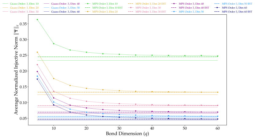
(a) MPS without translation-invariance compared to non-symmetrized complex Gaussian tensors.

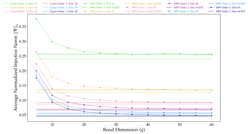
(a) MPS with translation-invariance compared to cyclically symmetrized complex Gaussian tensors.

Figure 14: Similar to the case with fixed bond dimension $q$ and increasing physical dimension $d$, when we fix the physical dimension $d$ and increase the bond dimension $q$, the entanglement increases. We compare order $3$ Gaussian MPS with and without translation-invariance, with cyclically symmetrized and non-symmetrized complex Gaussian tensors with the same physical (local) dimension $d$, respectively. In both cases, for a given $d$, as $q\to\infty$, the amount of entanglement present in the Gaussian MPS approaches that of the corresponding complex Gaussian tensor, hence supporting our claim.

Acknowledgements. K.F. thanks Rishika Bhagwatkar, Akshay Kulkarni, Aditya Shirwatkar, Prakrut Kotecha and Aaditya Rudra for timely assistance with running and monitoring the experiments. The authors were supported by the ANR project ESQuisses, grant number ANR-20-CE47-0014-01. K.F. acknowledges support from a NanoX project grant. C.L. and I.N. acknowledge support by the ANR project STARS, grant number ANR-20-CE40-0008, and by the PHC programs Sakura (Random Matrices and Tensors for Quantum Information and Machine Learning) and Procope (Entanglement Preservation in Quantum Information Theory). C.L. was also supported by the ANR project QTraj, grant number ANR-20-CE40-0024-01, while I.N. was also supported by the PHC Program Star (Applications of random matrix theory and abstract harmonic analysis to quantum information theory).

Appendix A Estimating the injective norm of deterministic multipartite pure states

As a part of our initial benchmarking experiments, we test the ALS and NGD algorithms on deterministic states for which the value of GME is well-known [ZCH10]. Here, we present mainly two types of states, namely generalized Dicke states and antisymmetric basis states.

A.1 Generalized Dicke states

Dicke states have found several applications in quantum communication and quantum networking [KST⁺07, PCT⁺09] along with some typical Dicke states being realized using trapped atomic ion systems [HCRW09]. Given an orthonormal basis $\{e_{1},e_{2},\ldots,e_{d}\}$ of $\mathbb{C}^{d}$, the associated generalized Dicke state $\Psi_{D}(n,d,\vec{k})\in\left(\mathbb{C}^{d}\right)^{\otimes n}$ is defined as

$$\Psi_{D}(n,d,\vec{k}):=\frac{1}{\sqrt{C_{n,d,\vec{k}}}}\;\sum_{\sigma\in S_{n,d,\vec{k}}}\overbrace{e_{\sigma(1)}\otimes\cdots\otimes e_{\sigma(1)}}^{k_{1}}\otimes\overbrace{e_{\sigma(2)}\otimes\cdots\otimes e_{\sigma(2)}}^{k_{2}}\otimes\cdots\otimes\overbrace{e_{\sigma(d)}\otimes\cdots\otimes e_{\sigma(d)}}^{k_{d}}$$ (18)

$$\vec{k}:=\left(k_{1},k_{2},\ldots,k_{d}\right),\quad\sum_{j=1}^{d}k_{j}=n,$$

where $S_{n,d,\vec{k}}$ denotes the set of all distinct permutations of the set $\{\overbrace{1,\ldots,1}^{k_{1}},\overbrace{2,\ldots,2}^{k_{2}},\ldots,\overbrace{d\ldots,d}^{k_{d}}\}$ and $C_{n,d,\vec{k}}=\frac{n!}{\prod_{j=1}^{d}k_{j}!}$ is the normalization factor. The analytical value for the GME of such states is known [ZCH10] and is given by

$$\operatorname{GME}\left(\Psi_{D}(n,d,\vec{k})\right)=\log\left[\frac{1}{C_{n,d,\vec{k}}}\prod_{j=1}^{d}\left(\frac{n}{k_{j}}\right)^{k_{j}}\right].$$ (19)

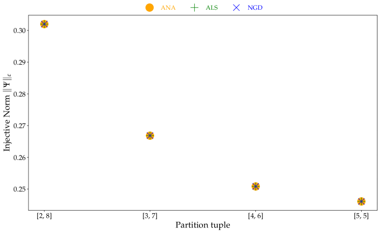
Figure 15: We consider generalized Dicke states with $n=10$ and $d=2$ as it holds physical relevance [HCRW09]. Both the ALS and NGD algorithms perform equally well at approximating the value of the normalized injective norm $\|\hat{\Psi}_{D}(10,2,\vec{k})\|_{\varepsilon}$, regardless of $\vec{k}$.

A.2 Antisymmetric basis states

Antisymmetric states have found substantial application in quantum cryptography [JABD03] and in the study of fermionic systems [ZCH10]. An antisymmetric pure state $\Psi_{A}\in\left(\mathbb{C}^{d}\right)^{\otimes n}$ is a normalized tensor such that every odd permutation of its tensor factors induces a sign change. The antisymmetric subspace of $\left(\mathbb{C}^{d}\right)^{\otimes n}$ is the collection of all pure antisymmetric tensors and has a dimension $\binom{d}{n}$, where $d\geq n$. The antisymmetric basis states can be constructed using the permutations of an orthonormal family $\{a_{1},\ldots,a_{n}\}$ of $\mathbb{C}^{d}$, as

$$\Psi_{A}(n,d):=\frac{1}{\sqrt{n!}}\sum_{\sigma\in S_{n}}\operatorname{sgn}(\sigma)a_{\sigma(1)}\otimes a_{\sigma(2)}\otimes\cdots\otimes a_{\sigma(n)},$$ (20)

where $S_{n}$ is the permutation group of $n$ elements, $\operatorname{sgn(\sigma)}$ is the sign of the permutation $\sigma$ and $\frac{1}{\sqrt{n!}}$ is the normalization factor. The analytical value for the GME of such state is known [ZCH10] and is given by

$$\operatorname{GME}\left(\Psi_{A}(n,d)\right)=\log(n!).$$ (21)

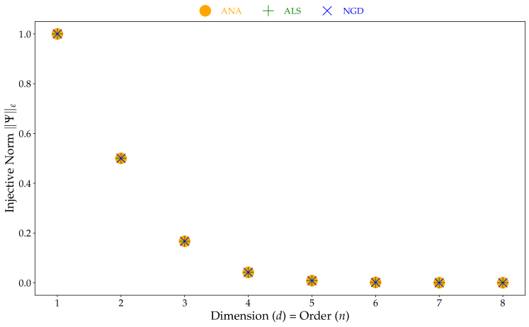
Figure 16: We consider antisymmetric basis states with $d=n$ from $1$ to $8$. Both the ALS and NGD algorithms perform equally well at approximating the value of the normalized injective norm $\|\hat{\Psi}_{A}(n,d)\|_{\varepsilon}$.

When benchmarking ALS and NGD on deterministic states, such as generalized Dicke states and antisymmetric basis states, we observe that both algorithms always perform equally well. This is in accordance with our observations in Section 4, namely that ALS and NGD have similar performances on normalized inputs. Now, let us emphasize that what we are interested in here is estimating the injective norm of specific tensors with fixed (in fact usually quite small) local dimension $d$. So there is no issue of having to deal with values that would go to $0$ as $d$ grows, as opposed to the case of random tensors, where we were trying to grasp the asymptotic values in the large dimension and/or order regime. In these kinds of situations, our tests suggest that one can indifferently use ALS and NGD.

The algorithms that we develop, mainly NGD and its symmetrized version SGD, can be used to approximate the injective norm of any tensor (SGD for any symmetrized tensor), real or complex, regardless of its number of tensor factors and its local dimension (provided sufficient computational resources). We have published our code with all the features used in this work as a Python library on an open-source repository along with installation instructions [FLN22]. Further, we will continue maintaining the repository and integrating new features based on community feedback.

References

- [ABAČ13] Antonio Auffinger, Gérard Ben Arous, and Jiří Černỳ. Random matrices and complexity of spin glasses. Communications on Pure and Applied Mathematics, 66(2):165–201, 2013.
- [AS17] Guillaume Aubrun and Stanisław J. Szarek. Alice and Bob Meet Banach: The Interface of Asymptotic Geometric Analysis and Quantum Information Theory, volume 223. American Mathematical Soc., 2017.
- [ASY14] Guillaume Aubrun, Stanislaw J. Szarek, and Deping Ye. Entanglement thresholds for random induced states. Communications on Pure and Applied Mathematics, 67(1):129–171, 2014.
- [BL01] Howard Barnum and Noah Linden. Monotones and invariants for multi-particle quantum states. Journal of Physics A: Mathematical and General, 34(35):6787, 2001.
- [CGGPG13] Benoît Collins, Carlos E. González-Guillén, and David Pérez-García. Matrix product states, random matrix theory and the principle of maximum entropy. Communications in Mathematical Physics, 320:663–677, 2013.
- [CKW00] Valerie Coffman, Joydip Kundu, and William K. Wootters. Distributed entanglement. Physical Review A, 61(5):052306, 2000.
- [CLDA09] Pierre Comon, Xavier Luciani, and André L. F. De Almeida. Tensor Decompositions, Alternating Least Squares and other Tales. Journal of Chemometrics, 23:393–405, 2009.
- [CN16] Benoit Collins and Ion Nechita. Random matrix techniques in quantum information theory. Journal of Mathematical Physics, 57(1), 2016.
- [DVC00] Wolfgang Dür, Guifre Vidal, and J. Ignacio Cirac. Three qubits can be entangled in two inequivalent ways. Physical Review A, 62(6):062314, 2000.
- [Evn21] Oleg Evnin. Melonic dominance and the largest eigenvalue of a large random tensor. Letters in Mathematical Physics, 111(3), 2021.
- [FLN22] Khurshed Fitter, Cecilia Lancien, and Ion Nechita. https://github.com/GlazeDonuts/Tensor-Norms, 2022.
- [GdOZ10] Silvano Garnerone, Thiago R. de Oliveira, and Paolo Zanardi. Typicality in random matrix product states. Physical Review A, 81(3):032336, 2010.
- [GGJN18] Carlos E. González-Guillén, Marius Junge, and Ion Nechita. On the spectral gap of random quantum channels. arXiv preprint arXiv:1811.08847, 2018.
- [Gro56] Alexandre Grothendieck. Résumé de la théorie métrique des produits tensoriels topologiques. Soc. de Matemática de São Paulo, 1956.
- [Har70] Richard A. Harshman. Foundations of the parafac procedure: Models and conditions for an "explanatory" multi-mode factor analysis. UCLA Working Papers in Phonetics, 16:1–84, 1970.
- [Has06] Matthew B. Hastings. Solving gapped hamiltonians locally. Phys. Rev. B, 73:085115, 2006.
- [Has09] Matthew B. Hastings. Superadditivity of communication capacity using entangled inputs. Nature Physics, 5(4):255–257, 2009.
- [HBRE21] Jonas Haferkamp, Christian Bertoni, Ingo Roth, and Jens Eisert. Emergent statistical mechanics from properties of disordered random matrix product states. PRX Quantum, 2:040308, 2021.
- [HCRW09] D. B. Hume, C. W. Chou, T. Rosenband, and D. J. Wineland. Preparation of dicke states in an ion chain. Physical Review A, 80(5), nov 2009.
- [HHHH09] Ryszard Horodecki, Paweł Horodecki, Michał Horodecki, and Karol Horodecki. Quantum entanglement. Reviews of Modern Physics, 81(2):865, 2009.
- [HL13] Christopher J Hillar and Lek-Heng Lim. Most tensor problems are np-hard. Journal of the ACM (JACM), 60(6):45, 2013.
- [JABD03] I. Jex, G. Alber, S.M. Barnett, and A. Delgado. Antisymmetric multi-partite quantum states and their applications. Fortschritte der Physik, 51(2-3):172–178, 2003.
- [KST+07] N. Kiesel, C. Schmid, G. Tóth, E. Solano, and H. Weinfurter. Experimental observation of four-photon entangled dicke state with high fidelity. Phys. Rev. Lett., 98:063604, Feb 2007.
- [LN] Cecilia Lancien and Ion Nechita. Estimating the injective norm of high-dimensional random tensors. work in progress.
- [LPG22] Cécilia Lancien and David Pérez-García. Correlation length in random mps and peps. Annales Henri Poincaré, 23(1):141–222, 2022.
- [LVV15] Zeph Landau, Umesh Vazirani, and Thomas Vidick. A polynomial time algorithm for the ground state of one-dimensional gapped local Hamiltonians. Nature Physics, 11:566–569, 2015.
- [PCT+09] R. Prevedel, G. Cronenberg, M. S. Tame, M. Paternostro, P. Walther, M. S. Kim, and A. Zeilinger. Experimental realization of dicke states of up to six qubits for multiparty quantum networking. Phys. Rev. Lett., 103:020503, Jul 2009.
- [PWB20] Amelia Perry, Alexander S. Wein, and Afonso S. Bandeira. Statistical limits of spiked tensor models. Annales de l’Institut Henri Poincaré, Probabilités et Statistiques, 56(1):230 – 264, 2020.
- [Rya13] Raymond A. Ryan. Introduction to tensor products of Banach spaces. Springer Science & Business Media, 2013.
- [Shi95] Abner Shimony. Degree of entanglement. Annals of the New York Academy of Sciences, 755(1):675–679, 1995.
- [TS14] Ryota Tomioka and Taiji Suzuki. Spectral norm of random tensors. arXiv preprint arXiv:1407.1870, 2014.
- [WC01] Alexander Wong and Nelson Christensen. Potential multiparticle entanglement measure. Physical Review A, 63(4):044301, 2001.
- [WG03] Tzu-Chieh Wei and Paul M. Goldbart. Geometric measure of entanglement and applications to bipartite and multipartite quantum states. Physical Review A, 68(4):042307, 2003.
- [ZCH10] Huangjun Zhu, Lin Chen, and Masahito Hayashi. Additivity and non-additivity of multipartite entanglement measures. New Journal of Physics, 12(8):083002, 2010.
- [ŻPNC11] Karol Życzkowski, Karol A Penson, Ion Nechita, and Benoit Collins. Generating random density matrices. Journal of Mathematical Physics, 52(6):062201, 2011.