Boost CTR Prediction for New Advertisements
via Modeling Visual Content

Abstract

Existing advertisements click-through rate (CTR) prediction models are mainly dependent on behavior ID features, which are learned based on the historical user-ad interactions. Nevertheless, behavior ID features relying on historical user behaviors are not feasible to describe new ads without previous interactions with users. To overcome the limitations of behavior ID features in modeling new ads, we exploit the visual content in ads to boost the performance of CTR prediction models. Specifically, we map each ad into a set of visual IDs based on its visual content. These visual IDs are further used for generating the visual embedding for enhancing CTR prediction models. We formulate the learning of visual IDs into a supervised quantization problem. Due to a lack of class labels for commercial images in advertisements, we exploit image textual descriptions as the supervision to optimize the image extractor for generating effective visual IDs. Meanwhile, since the hard quantization is non-differentiable, we soften the quantization operation to make it support the end-to-end network training. After mapping each image into visual IDs, we learn the embedding for each visual ID based on the historical user-ad interactions accumulated in the past. Since the visual ID embedding depends only on the visual content, it generalizes well to new ads. Meanwhile, the visual ID embedding complements the ad behavior ID embedding. Thus, it can considerably boost the performance of the CTR prediction models previously relying on behavior ID features for both new ads and ads that have accumulated rich user behaviors. After incorporating the visual ID embedding in the CTR prediction model of Baidu online advertising, the average CTR of ads improves by $1.46\%$, and the total charge increases by $1.10\%$.

I Introduction

Online advertising platforms serve personalized advertisements based on users’ potential interests. For example, Baidu Search Ads (a.k.a. “Phoenix Nest”) has been successfully using ultra-high dimensional input data and ultra-large-scale deep neural networks for training CTR (Click-Through Rate) models since 2013 [5, 51, 6]. In an advertising platform based on eCPM (effective Cost Per Mille), the advertisements fed to a specific user are ranked by the product of the bid price offered by the advertisers and the user’s predicted CTR from the CTR prediction model. Intuitively, it tends to put the advertisements with high predicted CTR and bid price at the top of the rank list to attract potential customers for advertisers and achieve high profit for the online advertising platform.

Since the predicted CTR has a substantial impact on the rank of the displayed ads, the deviation of the predicted CTR from the actual CTR has a significant influence on the revenue of advertisers and the advertising platform. If the predicted CTR of an ad is lower than the actual CTR, the ad might not get exposed to customers. In this case, the advertisers will not gain the expected revenues, and the advertising platform also loses the charges which it should have attained. On the other hand, if the predicted CTR of an ad is higher than the actual CTR, the ad will be misplaced at the top of the rank list but does not lead to the expected amount of clicks from customers. Then the advertisers will be overcharged by the advertising platform and cannot gain a reasonable profit. Thus, an effective CTR prediction model is a critical component for an eCPM advertising platform to achieve satisfactory advertising effects for the advertisers and abundant revenues for the advertising platform.

With the prompt progress achieved in machine learning in the past decade, we have witnessed the rapid evolution in the architecture of the CTR prediction model. The earliest works are mainly based on linear logistic regression (LR) model [21], non-linear gradient boosting decision trees (GBDT) [8, 23, 53, 22, 14, 24], Bayesian models [11] or factorization machines (FM) [34, 39, 15]. These models take a shallow structure and thus cannot effectively describe high-order latent patterns in the user-ad behavior. Inspired by the great success of deep learning in computer vision and natural language processing, researchers attempt to build deep neural networks (DNN) for CTR prediction. Factorization-machine supported neural network (FNN) [49] feeds the output of FM into a deep fully-connected neural network. Convolutional Click Prediction Model (CCPM) [27] predicts the CTR by a deep convolutional neural network. Zhang et al. [50] utilize the recurrent neural network to model the sequence of user behaviors for CTR prediction. The following works [2, 32, 12, 42, 41, 25, 38, 54, 16, 5, 7, 28, 51, 31, 36, 6, 45] explore more advanced neural networks for more effectively modeling higher-order patterns. Although extensive efforts have been devoted to improving the CTR prediction on the model side, the data side in the CTR prediction has been relatively less exploited. The lack of training data is commonly encountered for many machine learning tasks, including CTR prediction model training.

The existing mainstream CTR prediction model is based on the behavior ID features based on the historical interactions between users and ads. Each ad, as well as each user, is assigned a unique behavior ID. Each behavior ID of a user/ad is mapped to a vector, termed as embedding vector. The ad embedding vectors and user embedding vectors are learned jointly based on the historical behaviors of users on ads. Since the user/ad embedding vectors are learned based on historical behaviors, the quality of the learned features is heavily dependent on the richness of users’ past behaviors on ads. When a new ad is added to the advertising system, we have no access to the user-ad behavior on this new ad. It leads to the lack of the training data issue, and the behavior ID embedding for this new ad is not reliable at all for predicting the CTR of any user on the ad. The lack of training data for new ads is normally termed the cold-start problem.

A straightforward solution to solving the cold-start problem is using content-based features by understanding the visual content of ads [30, 10]. Specifically, Mo et al. [30] learn image features of display ads directly from raw pixels and user feedback in the target task. Ge et al. [10] exploits both ad image features and user behavior image features. Nevertheless, due to the high computational cost of image feature extraction, Mo et al. [30] and Ge et al. [10] adopt a pre-trained image feature extractor to get the image feature in the offline phase and then use the extracted image feature for predicting CVR/CTR in the online phase. Since the feature extractor is not related to CVR/CTR prediction in the training phase, the extracted image features might not be effective for CVR/CTR prediction. Zhao et al. [52] devise a pre-ranking model. When an advertiser uploads ads, the offline pre-ranking model determines inferior and superior ads based on their visual content. Only the superior ads with attractive visual content will be fed into the online ranker for further ad display. Since the pre-ranking model is conducted in the offline phase, the inefficiency caused by complex feature extraction is no longer an issue, and it makes the end-to-end training of feature extractor feasible. The offline pre-ranking model is trained by the accumulated historical data from all users in a learn-to-rank manner. Since the training data is collected from all users, it reveals the preference of the majority of users and might not reveal the preference of a specific user for personalized advertising.

In this work, we seek to model the visual content in ads for boosting the performance CTR prediction effectively. We map the visual content of an ad into a set of visual indices (IDs) through supervised clustering. After we obtain the visual IDs for ads, we learn a visual embedding vector for each visual ID based on the user’s clicks on ads. The learned visual ID embedding vector for each ad can effectively describe the visual content in an ad and can well generalize to ads newly added to the advertising system. Meanwhile, the visual content encoded in the visual ID embedding vector is complementary to the ad behavior ID embedding vector, which is beneficial to CTR prediction for not only new ads but also the ads which have accumulated rich user behaviors. In this case, as visualized in Figure 1, both ad behavior ID embedding and visual ID embedding are the input of the CTR prediction model, and they work together to achieve a more accurate CTR prediction.

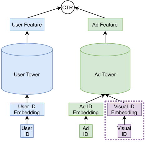
Figure 1: The structure of the proposed model. Different from the traditional CTR prediction model using only ad behavior ID embedding and user behavior ID embedding, our model additionally incorporates the visual content by devising a visual ID embedding for each ad (the purple rectangular). Since the visual ID embedding is only dependent on the visual content of the ad, it generalizes well for the new ads.

To generate the visual IDs for ads, a straightforward solution is using k-means to cluster the visual features from an off-the-shelf image feature extractor, e.g., a convolutional neural network. Nevertheless, the image features from the off-the-shelf image extractor such as ResNet-50 [13] pre-trained on ImageNet [3] might not be effective for discriminating the commercial images. To bridge the domain gap between the pre-trained dataset and the commercial application, we can fine-tune the pre-trained image extractor on commercial images in ads. Traditionally, fine-tuning the ResNet-50 requires human labours to annotate the label of each image, which is prohibitively expensive for the huge-scale commercial image corpus. Inspired by the recent success achieved by CLIP [33] in self-supervised learning, we exploit the textual description of the image in an ad as the supervision and construct a contrastive learning task to optimize the image feature extractor. After contrastive learning through supervision from textual descriptions of images, we can obtain the visual features. But it still deviates from our goal of obtaining the visual IDs. Thus, we devise a supervised clustering module based on the learned codebooks when fine-tuning the image feature extractor. Since the hard assignment in clustering is not differentiable, we soften the cluster assignment for achieving end-to-end training. Meanwhile, to enrich the codebooks for partitioning the visual feature space into finer cells, we adapt residual quantization and product quantization. After training the image feature extractor as well as the codebooks for supervised clustering using the textual description through contrastive learning, we use them to generate the visual IDs. The visual IDs are further mapped into visual ID embeddings, which will be the input of the CTR prediction model.

In summary, the contributions of this work are four-fold:

• We propose to incorporate visual content in the CTR prediction model through learning the visual ID embedding for ads. The learned visual ID embedding generalizes well to new ads and complements the ad behavior ID embedding.

• We devise an effective approach to learn the visual ID using the supervision from textual descriptions in a contrast-learning manner. We formulate the visual ID learning into a supervised clustering problem based on learned codebooks. To support end-to-end learning, we soften the cluster assignment and make it differentiable.

• To enrich the codebooks for partitioning the visual feature space into finer cells, we adopt both residual quantization and product quantization.

• We launched the proposed CTR prediction model incorporating the visual content in Baidu’s online advertising system. After launching, we achieved a $1.46\%$ improvement in CTR and a $1.10\%$ increase in total charges.

II Related Work

CTR prediction model. CTR prediction is a long-standing problem in online advertising and recommender system. The focus of CTR prediction is on learning an effective embedding for users as well as products (ads). Early works on embedding learning are mainly based on linear regression (LR) [17, 29, 1, 44] or factorization machine (FM) [20, 34, 35, 19, 15]. Specifically, LR-based methods use a linear projection to map the features into an embedding vector. The weights of the linear projection are optimized based on the binary cross-entropy loss. In parallel, FM-based methods map features into a latent space and model the interactions between users and products (ads) through the inner product of their embedding vectors. Inspired by the great success achieved by deep learning in computer vision [13] and natural language processing [40], several methods exploit deep neural networks to learn embedding vectors. Specifically, CNN-based CTR prediction model [27] exploits the interactions between neighbors in the feature space for enhancing the discriminating power of embedding features. Zhang et al. [49] utilizes deep neural networks to enhance the features from traditional embedding methods such as FMs, restricted Boltzmann machines (RBMs), and denoising auto-encoders (DAEs) for generating more effective embedding vectors. Wide$\&$Deep learning [2] jointly trains wide linear models and deep neural networks to combine their benefits for the recommender system. Product-based Neural Networks (PNN) [32] investigates the interactions between diffident features through inner-product and outer-product operations in neural networks for CTR prediction. Deep crossing [37] builds a deep neural network that automatically combines features to produce superior models. DeepFM [12] combines a factorization machine (FM) and a deep neural network (DNN). In DeepFM, the FM extracts low-order features, whereas the DNN generates the high-order features. DKN [41] develops a word-entity-aligned and knowledge-aware convolutional neural network to fuse s semantic-level and knowledge-level representations of news. Deep Interest Network (DIN) [55] models the user’s rich historical behaviors through a sequence model. Deep Interest Evolution Network (DIEN) [54] improves DIN by using a more advanced sequence model, GRU. Deep Session Interest Network (DSIN) [7] also focuses on modeling users’ behaviors in a sequence of sessions. It adopts Transformer [40], which has shown better performance than GRU in modeling sentences and documents. Search-based Interest Model (SIM) [31] models the user’s lifelong sequential behavior data through Transformer to exploit richer user behaviors. In these aforementioned methods, the CTR prediction is mainly based on the user’s ID embedding and the item’s ID embedding learned from the historical user behaviors. Thus, they might not perform well when the users’ historical behaviors are not sufficient. Different from above works, we utilize the visual content to complement the user’s ID embedding and the item’s ID embedding to achieve good CTR prediction performance for new ads and new users.

Visual features in CTR prediction. Mo et al. [30] feed the raw images in products (ads) into a convolutional neural network (CNN) and train the CNN through user-click supervision. It addresses the cold start problem when the ID features are not reliable when the historical behaviors are not rich enough. Ge et al. [10] extract image features not only on the products (ads) side but also on the user side. Zhao et al. [52] observes the efficiency problem encountered in [30, 10] and moves the image feature extractor to the offline phase. Specifically, before ranking the products (ads) through the CTR prediction model, they pre-rank the products (ads) based on their visual features. Category-specific CNN (CSCNN) [26] early fuses the product category with the visual image when modeling the product visual content and meanwhile devise an efficient architecture to make the online deployment of CNN model feasible. Wang et al. [43] proposes a hybrid bandit model using visual content as priors for creative ranking. Different from the above-mentioned methods, we map each ad into a visual ID. We train our image encoder and the visual ID generator based on the text-image pairs in an end-to-end manner. Then we learn the visual ID embedding using the objective of optimizing CTR prediction accuracy. Thus, our visual ID embedding not only encodes the visual content but also effectively describes the user-item interactions. Recently, the teams in Baidu Research and Baidu Search Ads developed a series of works [47, 48, 46] to exploit the use of vision BERT for boosting the text-visual relevance for video ads.

III Visual ID Generation

Supervision signal. We denote the image in the ad by $I$ and denote the visual index of the image by $\mathrm{ID}_{I}$. Straightforwardly, $\mathrm{ID}_{I}$ can be obtained from k-means clustering on ad image features extracted from an off-the-shelf image feature extractor, e.g., ResNet pre-trained on ImageNet dataset. Nevertheless, there is a domain gap between the natural images in ImageNet and the commercial images in the ads. A solution to adapting the target domain is fine-tuning the pre-trained ResNet on the commercial images in the ads. But there are no class labels available for supervising the network fine-tuning, and it is prohibitively expensive to annotate the image labels manually. Inspired by the great success achieved by CLIP [33] in self-supervised learning, we exploit the textual description of the images in the ad as the supervision to fine-tune the network through contrastive learning. We formulate the process of learning visual IDs for images in ads into a deep supervised clustering problem. Below we introduce the details.

Deep supervised clustering. We denote the textual description of the image $I$ by $T$. We denote the image feature extractor by $\mathrm{Encoder}_{\mathrm{img}}$ and that for encoding the textual description by $\mathrm{Encoder}_{\mathrm{txt}}$. We denote the image feature of $I$ generated from $\mathrm{Encoder}_{\mathrm{img}}$ by $\mathbf{x}\in\mathbb{R}^{d}$ and the text feature of $T$ from $\mathrm{Encoder}_{\mathrm{txt}}$ by $\mathbf{y}\in\mathbb{R}^{d}$. That is,

$$\mathbf{x}=\mathrm{Encoder}_{\mathrm{img}}(I),\mathbf{y}=\mathrm{Encoder}_{\mathrm{txt}}(T).$$ (1)

To make the clustering feasible, we devise a dictionary denoted by $\mathcal{C}=\{\mathbf{c}_{i}\}_{i=1}^{N}$. $\mathcal{C}$ are weights of the network which are randomly initialized and optimized through contrastive learning. Straightforwardly, we can map the visual feature $\mathbf{x}$ from the image extractor to its closest codeword in $\mathcal{C}$. In this case, the visual ID of the image $I$ is just the index of its closest codeword:

$$\mathrm{ID}_{I}=\mathrm{argmax}_{i\in[1,N]}-\|\mathbf{c}_{i}-\mathbf{x}\|_{2},$$ (2)

where $\|.\|_{2}$ denotes the $L_{2}$ norm. The visual feature $\mathbf{i}$ is mapped to $\mathbf{c}_{\mathrm{ID}_{I}}$ to learn $\mathbf{C}$ through contrastive learning. Nevertheless, the above formulation can only optimize $\mathbf{C}$ but fail to back-propagate the gradient to update the image encoder due to the fact that the hard assignment in Eq. (2) is not differentiable. Thus, we soften the hard assignment and map the image feature $\mathbf{x}$ into a weighted summation of codewords:

$$\hat{\mathbf{x}}=\sum_{i=1}^{N}s_{i}\mathbf{c}_{i},$$ (3)

where $s_{i}$ is the weight computed by

$$s_{i}=\frac{e^{-\beta\|\mathbf{x}-\mathbf{c}_{i}\|_{2}}}{\sum_{j=1}^{N}e^{-\beta\|\mathbf{x}-\mathbf{c}_{j}\|_{2}}},$$ (4)

where $\beta$ is a pre-defined positive constant controlling the softness of the assignment. When $\beta\to+\infty$, the soft-assignment operation in Eq. (3) will degenerate to the hard assignment. To approximate the hard assignment well, $\beta$ cannot be set to be a small value. On the other hand, if $\beta$ is too large, the softmax function in Eq. (3) tends to fall into the saturation region and leads to gradient vanishing. In implementation, we set $\beta$ to be a small value in the first epoch and gradually increases it to a large value in the training process.

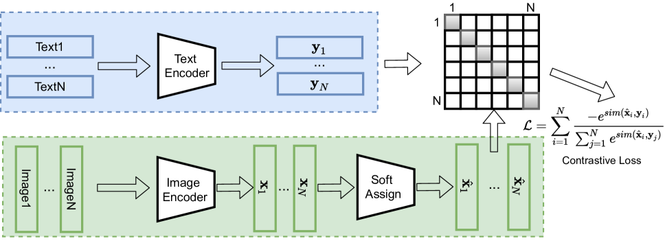
Figure 2: The pipeline of learning visual IDs. Given a batch of $N$ text-image pairs. An image is only relevant with the text in the pair and is irrelevant with other $N-1$ images. The text extractor generates the text features $\{\mathbf{y}_{i}\}_{i=1}^{N}$ and the image extractor generates the image features $\{\mathbf{x}_{i}\}_{i=1}^{N}$. An image feature $\mathbf{x}_{i}$ is mapped into a weighted summation of its neighboring codewords $\hat{\mathbf{x}}_{i}$ through the soft assignment. Then the similarity between the text features $\{\mathbf{y}_{i}\}_{i=1}^{N}$ and the mapped image codewords $\{\hat{\mathbf{x}}_{i}\}_{i=1}^{N}$ are optimized through the contrastive loss.

To partition the feature space into a fine level, we need to set the number of codewords in the codebook $\mathbf{C}$ large enough. Nevertheless, the increase in the number of codewords will inevitably lead to an increase in memory and computation costs. To achieve high efficiency, we conduct a two-level quantization by exploiting residual quantization. In the first level, we map the feature $\mathbf{x}$ into codewords from the coarse-level dictionary $\mathcal{C}_{0}=\{\mathbf{c}_{0,i}\}_{i=1}^{N_{0}}$ in a soft-assignment manner:

$$\bar{\mathbf{x}}=\sum_{i=1}^{N_{0}}s_{0,i}\mathbf{c}_{0,i},$$ (5)

where

$$s_{0,i}=\frac{e^{-\beta\|\mathbf{x}-\mathbf{c}_{0,i}\|_{2}}}{\sum_{j=1}^{N}e^{-\beta\|\mathbf{x}-\mathbf{c}_{0,j}\|_{2}}},$$ (6)

Then we compute the residual vector $\mathbf{r}$:

$$\mathbf{r}=\mathbf{x}-\hat{\mathbf{x}}.$$ (7)

After that, we conduct product quantization (PQ) [18, 9] to split the image residual features $\mathbf{r}\in\mathbb{R}^{d}$ into $K$ segments:

$$\mathbf{r}\to[\mathbf{r}_{1},\cdots,\mathbf{r}_{K}],$$ (8)

and each segment of the residual vector $\mathbf{r}_{k}\in\mathbb{R}^{\frac{d}{K}}$, $\forall k\in[1,K]$. We conduct clustering on each split segment of the residual vector $\mathbf{r}_{k}$ based on the split-specific codebook $\mathcal{C}_{k}=\{\mathbf{c}_{k,i}\}_{i=1}^{N_{k}}$, where $\mathbf{c}_{k,i}\in\mathbb{R}^{\frac{d}{K}}$. To be specific, we conduct

$$\bar{\mathbf{r}}_{k}=\sum_{i=1}^{N_{k}}s_{k,i}\mathbf{c}_{k,i},$$ (9)

where

$$s_{k,i}=\frac{e^{-\beta\|\mathbf{r}_{k}-\mathbf{c}_{k,i}\|_{2}}}{\sum_{j=1}^{N}e^{-\beta\|\mathbf{r}_{k}-\mathbf{c}_{k,j}\|_{2}}}.$$ (10)

After that, $\{\hat{\mathbf{r}}_{k}\}_{k=1}^{K}$ are concatenated into the recovered residual feature:

$$\hat{\mathbf{r}}\leftarrow[\hat{\mathbf{r}}_{1},\cdots,\hat{\mathbf{r}}_{K}].$$ (11)

The recovered feature vector is obtained by summing up the recovered residual feature $\hat{\mathbf{r}}$ and coarse-quantize vector $\bar{\mathbf{x}}$ in Eq. (5):

$$\hat{\mathbf{x}}=\hat{\mathbf{r}}+\bar{\mathbf{x}}.$$ (12)

Straightforwardly, the coarse-level codebook $\mathcal{C}_{0}$ and $K$ fine-level sub-codebooks $\{\mathbf{C}_{k}\}_{k=1}^{K}$ can partition the whole feature space into $\prod_{k=0}^{K}N_{k}$ cells. But the total memory complexity of storing the codebooks $\{\mathbf{C}_{k}\}_{k=0}^{K}$ is only $\mathcal{O}(dN)$.

Contrastive learning. The contrastive learning is conducted within each mini-batch. Given a mini-batch of text-image pairs $\{(I_{i},T_{i})\}_{i=1}^{B}$, the image $I_{i}$ is only relevant with the text $T_{i}$ and is irrelevant with other texts, $T_{j}$ ($j\neq i$). Thus, after we obtain the text features $\{\mathbf{y}_{i}\}_{i=1}^{B}$ and the mapped image features $\{\hat{\mathbf{x}}_{i}\}_{i=1}^{B}$ from the codebooks $\{\mathcal{C}\}_{k=0}^{K}$ based on Eq. (3)-(12), we construct the contrastive loss defined as

$$\mathcal{L}=$$ (13)

$$-\frac{1}{B}\sum_{i=1}^{B}\left\{\mathrm{log}(\frac{e^{\mathrm{sim}(\hat{\mathbf{x}}_{i},\mathbf{y}_{i})}}{\sum_{j=1}^{B}e^{\mathrm{sim}(\hat{\mathbf{x}}_{j},\mathbf{y}_{i})}})+\mathrm{log}(\frac{e^{\mathrm{sim}(\hat{\mathbf{x}}_{i},\mathbf{y}_{i})}}{\sum_{j=1}^{B}e^{\mathrm{sim}(\hat{\mathbf{x}}_{i},\mathbf{y}_{j})}})\right\},$$

where $\mathrm{sim}(\cdot,\cdot)$ is the function measuring the cosine similarity between two vectors defined as

$$\mathrm{sim}(\mathbf{x},\mathbf{y})=\frac{\mathbf{x}^{\top}\mathbf{y}}{\|\mathbf{x}\|_{2}\|\mathbf{y}\|_{2}}.$$ (14)

The contrastive learning loss aims to enlarge the gap between similarities of positive pairs and those of negative pairs. The process of learning image encoder, text encoder and dictionaries are visualized in Figure 2 and summarized in Algorithm 1.

Algorithm 1 Image encoder and dictionary learning.

Input: The image encoder $\mathrm{Encoder}_{\mathrm{img}}$, the text encoder $\mathrm{Encoder}_{\mathrm{txt}}$, $K+1$ codebooks $\{\mathcal{C}_{k}\}_{k=0}^{K}$, and text-image pairs $\{I_{i},T_{i}\}_{i=1}^{B}$, the positive constant $\beta$.

for $i\ \in[1,B]$

$\mathbf{x}_{i}\leftarrow\mathrm{Encoder}_{\mathrm{img}}(I_{i})$

$\mathbf{y}_{i}\leftarrow\mathrm{Encoder}_{\mathrm{txt}}(T_{i})$

$\bar{\mathbf{x}}_{i}=\sum_{j=1}^{N}\mathbf{c}_{0,j}\frac{e^{-\beta\|\mathbf{x}-\mathbf{c}_{0,j}\|_{2}}}{\sum_{l=1}^{N}e^{-\beta\|\mathbf{x}-\mathbf{c}_{0,l}\|_{2}}}$

$\mathbf{r}_{i}\leftarrow\mathbf{x}_{i}-\bar{\mathbf{x}}_{i}$

$[\mathbf{r}_{i,1},\cdots,\mathbf{r}_{i,K}]\leftarrow\mathbf{r}_{i}$
for $k\ \in[1,K]$

$\hat{\mathbf{r}}_{i,k}=\sum_{j=1}^{N}\mathbf{c}_{1,j}\frac{e^{-\beta\|\mathbf{r}_{i,k}-\mathbf{c}_{k,j}\|_{2}}}{\sum_{l=1}^{N}e^{-\beta\|\mathbf{r}_{i,k}-\mathbf{c}_{k,l}\|_{2}}}$

$\hat{\mathbf{r}}_{i}\leftarrow[\hat{\mathbf{r}}_{i,1},\cdots,\hat{\mathbf{r}}_{i,K}]$    $\hat{\mathbf{x}}_{i}\leftarrow\hat{\mathbf{r}}_{i}+\bar{\mathbf{x}}_{i}$
$\mathcal{L}=\frac{-1}{B}\sum_{i=1}^{B}\mathrm{log}\left(\frac{e^{\frac{\hat{\mathbf{x}}_{i}^{\top}\mathbf{y}_{i}}{\|\mathbf{x}_{i}\|_{2}\|\mathbf{y}_{i}\|_{2}}}}{\sum_{j=1}^{B}e^{\frac{\hat{\mathbf{x}}_{i}^{\top}\mathbf{y}_{j}}{\|\mathbf{x}_{i}\|_{2}\|\mathbf{y}_{j}\|_{2}}}}\right)$

Update $\mathrm{Encoder}_{\mathrm{img}}$, $\mathrm{Encoder}_{\mathrm{txt}}$, the codebooks $\{\mathcal{C}_{k}\}_{k=0}^{K}$ based on $\mathcal{L}$ using stochastic gradient descent.

Visual ID generation. After we train the models using the contrastive learning, we use the image encoder $\mathrm{Encoder}_{\mathrm{img}}$ to extract the image feature $\mathbf{x}$. Then $\mathbf{x}$ is mapped to its closest codewords in the learned coarse-level dictionary $\mathcal{C}_{0}=\{\mathbf{c}_{0,i}\}_{i=1}^{N_{0}}$. We define the index of the mapped codeword in $\mathcal{C}_{0}$ as the visual ID $\mathrm{ID}_{0}^{v}$. Then, we compute the residual feature vector $\mathbf{r}=\mathbf{x}-\mathbf{c}_{0,\mathrm{ID}_{0}^{v}}$. After that, $\mathbf{r}$ is equally split into $K$ segments $\{r_{k}\}_{k=1}^{K}$, and each segment is mapped to its closest codeword in the codebook $\mathbf{C}_{k}=\{\mathbf{c}_{k,i}\}_{i=1}^{N_{k}}$. We define the index of the closest codeword in each dictionary $\mathbf{C}_{k}$ as the visual ID $\mathrm{ID}_{k}^{v}$, that is,

$$\begin{split}\mathrm{ID}_{k}^{v}=\mathrm{argmin}_{i}{\|\mathbf{r}_{k}-\mathbf{c}_{k,i}\|}.\\ \end{split}$$ (15)

We visualize the process of generating visual ID in Figure 3. In total, for each image, we generate $K+1$ visual IDs ($\{\mathrm{ID}_{k}^{v}\}_{k=0}^{K}$), which will be used as the input of the CTR model to encode the visual content of the ad. It is worth noting that, the image extractor $\mathrm{Encoder}_{\mathrm{img}}$ and $K+1$ codebooks $\{\mathcal{C}_{k}\}_{k=0}^{K}$ are only used in generating visual ID. They will not be involved when learning the visual ID embedding for CTR prediction. An alternative choice is to plug the image extractor $\mathrm{Encoder}_{\mathrm{img}}$ and the codebooks $\{\mathcal{C}_{k}\}_{k=0}^{K}$ into the CTR prediction model to achieve end-to-end training. But it is prohibitively expensive due to the fact that the image feature extractor is normally heavy.

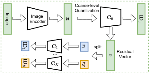
Figure 3: The pipeline of generating visual IDs. An image is fed into the image encoder to generate the image feature $\mathbf{x}$. It first finds its closest codeword in the coarse-level codebook $\mathcal{C}_{0}=\{\mathbf{c}_{0,i}\}_{i=1}^{N_{0}}$ and the index of the losest codeword is the first visual ID, $\mathrm{ID}_{0}$. Meanwhile, we obtain the residual vector $\mathbf{r}=\mathbf{x}-\mathbf{c}_{0,\mathrm{ID}_{0}}$, which is equally split into $K$ segments $[\mathbf{r}_{1},\cdots,\mathbf{r}_{K}]$. Each segment $\mathbf{r}_{k}$ is mapped to its closest codeword in the dictionary $\mathbf{C}_{k}$ and the index of the closest codeword in $\mathbf{C}_{k}$ corresponds to the visual ID, $\mathrm{ID}_{K}$. In total, we obtain $K+1$ visual IDs for an image.

IV CTR Prediction Model Learning

The CTR prediction model in our advertising platform takes the user ID, the ad ID and the ad visual ID as input to predict the CTR. We denote a user by $u$ and an ad by $a$. The CTR prediction model consists of embedding layers, the ad tower, the user tower and the prediction head. To be specific, the user embedding layer maps the ID of the user $u$ to a vector:

$$\mathbf{u}=\mathrm{EMB}_{\mathrm{user}}(\mathrm{ID}_{u}),$$ (16)

the ad embedding layer maps the ID of the ad $a$ to a vector:

$$\mathbf{a}=\mathrm{EMB}_{\mathrm{ad}}(\mathrm{ID}_{a}).$$ (17)

The visual embedding layer maps the ad’s each visual IDs $\mathrm{ID}^{v}_{k}$ ($k\in[0,K]$) to a feature vector in the following manner

$$\begin{split}{\mathbf{x}}&=\mathrm{EMB}_{\mathrm{visual}}^{(0)}(\mathrm{ID}^{v}_{0})\\ \mathbf{r}_{k}&=\mathrm{EMB}_{\mathrm{visual}}^{(k)}(\mathrm{ID}^{v}_{k}),~{}\forall k\in[1,K].\\ \end{split}$$ (18)

Then the visual embedding of the ad $\mathbf{v}$ is obtained by concatenating $\{\mathbf{r}_{k}\}$ and summing up the concatenated vector with ${\mathbf{x}}$

$$\begin{split}\mathbf{r}&=[\mathbf{r}_{1},\cdots,\mathbf{r}_{K}],\\ \mathbf{v}&=\mathbf{x}+\mathbf{r}.\\ \end{split}$$ (19)

The user tower takes $\mathbf{u}$ as input, and generates the user feature:

$$\hat{\mathbf{u}}=\mathrm{Tower}_{\mathrm{user}}(\mathbf{u}).$$ (20)

In parallel, the ad tower takes $\mathbf{a}$ and $\mathbf{v}$ as input, and generates the ad feature:

$$\hat{\mathbf{a}}=\mathrm{Tower}_{\mathrm{ad}}([\mathbf{a},\mathbf{v}]).$$ (21)

In practice, both $\mathrm{Tower}_{\mathrm{ad}}$ and $\mathrm{Tower}_{\mathrm{user}}$ are implemented by several fully-connected layers. The prediction head takes the user feature $\hat{\mathbf{u}}\in\mathbb{R}^{D}$ and the ad feature $\hat{\mathbf{a}}\in\mathbb{R}^{D}$ as input and generates the predicted CTR:

$$\hat{y}=\mathrm{sigmoid}([\hat{\mathbf{u}},\hat{\mathbf{a}}]\mathbf{w}+b),$$ (22)

where $\mathbf{w}\in\mathbb{R}^{2D}$ and $b\in\mathbb{R}$ are weights of the prediction head, and $\mathrm{sigmoid}$ is the function defined as $\mathrm{sigmoid}(x)=\frac{1}{1+e^{-x}}$. In the training phase, we construct a binary cross-entropy loss to update the weights CTR prediction model. To be specific, given the predicted CTR $\hat{y}\in(0,1)$ and the ground-truth CTR by $y\in\{0,1\}$, the binary cross-entropy loss is constructed by

$$\mathcal{L}_{\mathrm{BCE}}=-[(1-y)\mathrm{log}(\hat{y})+y\mathrm{log}(1-\hat{y})].$$ (23)

Algorithm 2 CTR prediction model learning.

Input: The user-ad pairs $\{a_{i},u_{i}\}_{i=1}^{M}$ and the ground-truth labels $\{y_{i}\}_{i=1}^{M}$, user embedding layer $\mathrm{EMB}_{\mathrm{user}}$, ad embedding layer $\mathrm{EMB}_{\mathrm{ad}}$, and visual embedding layers $\mathrm{EMB}_{\mathrm{visual}}^{(1)}$ and $\mathrm{EMB}_{\mathrm{visual}}^{(2)}$, user tower $\mathrm{Tower}_{\mathrm{user}}$, ad tower $\mathrm{Tower}_{\mathrm{ad}}$, the prediction head with weights $\{\mathbf{w},b\}$

for  $i\ \in[1,M]$

fetch the ad ID for $a_{i}$, $\mathrm{ID}_{a}$

$\mathbf{a}=\mathrm{EMB}_{\mathrm{ad}}(\mathrm{ID}_{a})$

fetch the visual IDs of $a_{i}$, $\{\mathrm{ID}^{v}_{k}\}_{k=0}^{K}$

$\mathbf{x}=\mathrm{EMB}_{\mathrm{visual}}^{(0)}(\mathrm{ID}_{0}^{v})$

for  $k\ \in[1,K]$

$\mathbf{r}_{k}=\mathrm{EMB}_{\mathrm{visual}}^{(k)}(\mathrm{ID}_{k}^{v})$

$\mathbf{r}=[\mathbf{r}_{1},\cdots,\mathbf{r}_{K}]$

$\mathbf{v}=\mathbf{r}+\mathbf{x}$

$\hat{\mathbf{a}}=\mathrm{Tower}_{\mathrm{ad}}([\mathbf{a},\mathbf{v}]$

fetch the user ID for $u_{i}$, $\mathrm{ID}_{u}$

$\mathbf{u}=\mathrm{EMB}_{\mathrm{user}}(\mathrm{ID}_{u})$

$\hat{\mathbf{u}}=\mathrm{Tower}_{\mathrm{user}}(\mathbf{u})$

$\hat{y}_{i}=\mathrm{sigmoid}([\hat{\mathbf{u}},\hat{\mathbf{a}}]\mathbf{w}+b),$

$\mathcal{L}=-\frac{1}{M}\sum_{i=1}^{M}(1-y_{i})\mathrm{log}(\hat{y}_{i})+y_{i}\mathrm{log}(1-\hat{y}_{i})$

Update $\mathrm{EMB}_{\mathrm{user}}$, $\mathrm{EMB}_{\mathrm{ad}}$, $\mathrm{EMB}_{\mathrm{visual}}^{(1)}$, $\mathrm{EMB}_{\mathrm{visual}}^{(2)}$, $\mathrm{Tower}_{\mathrm{user}}$, $\mathrm{Tower}_{\mathrm{ad}}$, $\mathbf{w}$, and $b$ using $\mathcal{L}$ by stochastic gradient descent.

Algorithm 2 summarizes the CTR prediction model learning.

V Experiments

Implementation. We implement the image encoder $\mathrm{Encoder}_{\mathrm{img}}$ by ResNet50 [13] with $50$ layers and the text encoder $\mathrm{Encoder}_{\mathrm{txt}}$ by the BERT-base model [4] with $12$ Transformer layers and $768$ hidden size. ResNet50 is pre-trained on ImageNet dataset and the BERT-base model is pre-trained on sentences from the BooksCorpus dataset with 800 Million words and English Wikipedia with 2,500 million words. We use the hidden feature before the last classification layer of ResNet50 as the image feature $\mathbf{x}$ and use the hidden state of the [cls] token in the last layer of the BERT-base as the text feature $\mathbf{y}$. To make the dimension of the image feature identical to that of the text feature, we add a fully-connected layer to project the feature obtained from the ResNet to the $768$-dimensional vector. By default, we set the number of codebooks for the residual vector, $K$, as $4$. Meanwhile we set the default number of codewords in each codebook $\mathcal{C}_{k}$, $N_{k}$, as $256$. In the training process, we set the initial value of $\beta$ as $1$ and gradually increase it to $10$.

Training data. To train the image extractor $\mathrm{Encoder}_{\mathrm{img}}$, the text extractor $\mathrm{Encoder}_{\mathrm{txt}}$ and the codebooks $\{\mathcal{C}_{k}\}_{k=0}^{K}$, we use $50$ million text-image pairs collected from our advertising system. To train the CTR prediction model, we use $70$ million user-click data per day collected from our advertising system and the model is fine-tuned for around 1 month.

V-A Offline Experiments

We evaluate the influence of our model on the CTR prediction in the offline phase. We first define the CTR prediction model using only ad behavior ID features and user behavior ID features as the baseline. We use the AUC improvement of CTR prediction over the baseline model as the evaluation metrics. Meanwhile, we use an observation window of 40-day length to demonstrate more details.

Residual quantization. By default, we conduct a two-level residual quantization. In the first level, we conduct a coarse level quantization using $\mathcal{C}_{0}$ and then conduct the second-level quantization on the residual. Here, we compare the two-level residual quantization with a single-level quantization by removing the first-level coarse level quantization. We report the AUC difference between the model with the baseline model along $40$ days in Figure 4.

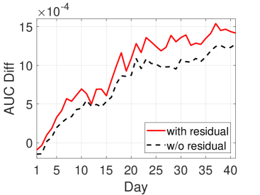
Figure 4: Comparisons with the setting without residual quantization.

As shown in the figure, using the residual quantization, the model can get more improvement compared with its counterpart without residual quantization. To be specific, at the $40$-th day, using residual quantization, the model achieves a $0.1418\%$ AUC improvement, whereas the model without residual quantization only achieves a $0.1242\%$ AUC increase.

Comparisons with alternative configurations. We soften the quantization operation as Eq. (3) and Eq. (4) to make it differentiable. Thus, the codeword assignment can be incorporated into a neural network, and the codewords can be learned in an end-to-end manner. An alternative solution is a two-stage learning process. In the first stage, we can learn the raw feature vectors without quantization through the contrastive loss based on the text-image pairs. After that, we use the unsupervised k-means clustering to conduct residual quantization and product quantization for generating the codebooks and the visual IDs. We term this configuration as the two-stage baseline. Meanwhile, we also compare with the baseline directly using the raw feature vectors learned without quantization through the contrastive loss based on text-image pairs as the visual representation for CTR prediction. We term it as w/o quantization baseline. As shown in Figure 5, ours consistently outperforms two compared baselines, demonstrating the effectiveness of learning codebooks in an end-to-end manner.

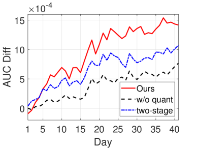
Figure 5: Comparisons with the two-stage setting and the setting without quantization.

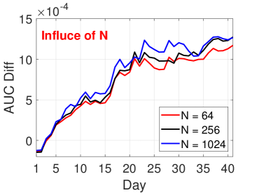
(a) The influence of $N$

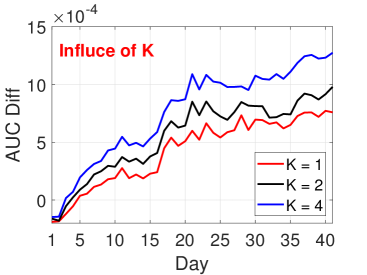
(b) The influence of $K$

Figure 6: The influence of parameters on the performance.

(a) $\mathrm{ID}^{v}_{0}=1388$, $\mathrm{ID}^{v}_{1}=145$, $\mathrm{ID}^{v}_{2}=251$, $\mathrm{ID}^{v}_{3}=86$, $\mathrm{ID}^{v}_{4}=87$

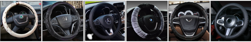
(b) $\mathrm{ID}^{v}_{0}=1511$, $\mathrm{ID}^{v}_{1}=201$, $\mathrm{ID}^{v}_{2}=106$, $\mathrm{ID}^{v}_{3}=42$, $\mathrm{ID}^{v}_{4}=149$

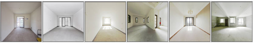
(c) $\mathrm{ID}^{v}_{0}=84$, $\mathrm{ID}^{v}_{1}=104$, $\mathrm{ID}^{v}_{2}=61$, $\mathrm{ID}^{v}_{3}=22$, $\mathrm{ID}^{v}_{4}=202$

Figure 7: Visualization of ads with the same visual IDs.

Influence of the number of codewords. A larger number of codewords can partition the feature space into finer cells and leads to smaller quantization errors. We evaluate the influence of the number of codewords, $N$, on the AUC of CTR prediction. To this end, we show the results when $N$ varies among $\{64,256,1024\}$. As shown in Figure 6 (a), when $N$ increases from $64$ to $256$, the AUC of CTR prediction gets improved considerably. But when $N$ further increases to $1024$, the AUC gets saturated. Since the increase of $N$ will bring more computation cost, considering both efficiency and effectiveness, we set $N=256$ by default.

Influence of the number of segments. We split the residual vector into $K$ segments and conduct product quantization based on split segments. A larger $K$ also leads to a finer partition of the feature space and smaller quantization errors. We evaluate the influence of the number of segments, $K$, on the AUC of CTR prediction. To this end, we show the results when $K$ is chosen from $\{1,2,4\}$. As shown in Figure 6 (b), when $K$ increases from $1$ to $4$, the AUC of CTR prediction gets boosted significantly. To be specific, when $K=1$, at the $40$-th day, the AUC improvement over baseline is only $0.0903\%$, whereas the AUC improvement is $0.1418\%$ when $K=4$. But the increase of $K$ also brings more computational cost. Thus, to balance the efficiency and effectiveness, we do not further increase $K$ beyond $4$ and set $K=4$, by default.

Influence on new ads and old ads. As we know, incorporating the visual content cannot bring more benefits to new ads since their ID features are not reliable. Here, we demonstrate the influence of our model in new ads and the old ones. As shown in Table I, using the visual ID embedding, it has a more influential impact on new ads than old ads. To be specific, for new ads, it brings $+0.6098\%$ increase in AUC of the CTR prediction, whereas it only brings $+0.1238\%$ increase for old ads.

TABLE I: The influence of visual ID embedding on new ads and old ads.

old ads		new ads
# of instances	AUC diff	# of instances	AUC diff
$61,982,597$	$+0.1238\%$	$4,935,208$	$+0.6098\%$

Visualization. In Figure 7, we visualize the ads with the same visual IDs, $\{\mathrm{ID}_{k}^{v}\}_{k=0}^{4}$. It is not difficult to observe from the figure that the ads with the same visual IDs have a similar visual appearance, demonstrating the effectiveness of the learned visual IDs.

V-B Online Experiments

TABLE II: The influence of launching the proposed model in our advertising platform. Note that “$+\cdot\%$” is relative improvement for online experiments.

Charge	CTR
$+1.10\%$	$+1.46\%$

In Table II, we show the influence of launching the proposed model in Baidu online advertising platform. Before launching our model, the CTR prediction model in our advertising platform uses only the ad ID features and user ID features based on the users’ historical behaviors. As shown in the table, after launching our model, the charge of our advertising platform gets increased relatively by $+1.10\%$, and the CTR of the ads gets improved relatively by $+1.46\%$. That is, the launching of the proposed model brings significant revenue boosts for the advertisers as well as our ads platform.

VI Conclusion

The traditional CTR prediction model relies on the user behavior ID features and product (ad) behavior ID features. But the effectiveness of these ID features requires rich historical user-product (ad) behaviors, and thus they do not generalize well to the new products (ads). In this work, we investigate exploiting visual content in ads to boost the CTR prediction accuracy. We adopt the textual description of images as the supervision to learn the image feature extractor and map the visual content in each ad to visual IDs. Then we learn the embedding for visual IDs based on the user’s clicking behaviors. We feed the learned visual ID embedding besides the ad behavior ID embedding and the user behavior ID embedding into a CTR prediction model to generate a more reliable CTR prediction. The systematic offline experiments demonstrate the improved AUC of the CTR prediction by incorporating the visual content. After launching the proposed model in Baidu advertising platform, we achieve a $1.10\%$ charge increase and a $1.46\%$ CTR increase.

References

- [1] Olivier Chapelle. Modeling delayed feedback in display advertising. In Proceedings of the 20th ACM SIGKDD International Conference on Knowledge Discovery and Data Mining (KDD), pages 1097–1105, New York, NY, 2014.
- [2] Heng-Tze Cheng, Levent Koc, Jeremiah Harmsen, Tal Shaked, Tushar Chandra, Hrishi Aradhye, Glen Anderson, Greg Corrado, Wei Chai, Mustafa Ispir, et al. Wide & Deep Learning for Recommender Systems. In Proceedings of the 1st Workshop on Deep Learning for Recommender Systems (DLRS), pages 7–10, Boston, MA, 2016.
- [3] Jia Deng, Wei Dong, Richard Socher, Li-Jia Li, Kai Li, and Fei-Fei Li. Imagenet: A large-scale hierarchical image database. In Proceedings of the 2009 IEEE Computer Society Conference on Computer Vision and Pattern Recognition (CVPR), pages 248–255, Miami, FL, 2009.
- [4] Jacob Devlin, Ming-Wei Chang, Kenton Lee, and Kristina Toutanova. BERT: pre-training of deep bidirectional transformers for language understanding. In Proceedings of the 2019 Conference of the North American Chapter of the Association for Computational Linguistics: Human Language Technologies (NAACL-HLT), pages 4171–4186, Minneapolis, MN, 2019.
- [5] Miao Fan, Jiacheng Guo, Shuai Zhu, Shuo Miao, Mingming Sun, and Ping Li. MOBIUS: towards the next generation of query-ad matching in baidu’s sponsored search. In Proceedings of the 25th ACM SIGKDD International Conference on Knowledge Discovery & Data Mining (KDD), pages 2509–2517, Anchorage, AK, 2019.
- [6] Hongliang Fei, Jingyuan Zhang, Xingxuan Zhou, Junhao Zhao, Xinyang Qi, and Ping Li. GemNN: Gating-enhanced multi-task neural networks with feature interaction learning for CTR prediction. In Proceedings of the 44th International ACM SIGIR Conference on Research and Development in Information Retrieval (SIGIR), pages 2166–2171, Virtual Event, Canada, 2021.
- [7] Yufei Feng, Fuyu Lv, Weichen Shen, Menghan Wang, Fei Sun, Yu Zhu, and Keping Yang. Deep session interest network for click-through rate prediction. In Proceedings of the Twenty-Eighth International Joint Conference on Artificial Intelligence (IJCAI), pages 2301–2307, Macao, China, 2019.
- [8] Jerome H. Friedman. Greedy function approximation: A gradient boosting machine. The Annals of Statistics, 29(5):1189–1232, 2001.
- [9] Tiezheng Ge, Kaiming He, Qifa Ke, and Jian Sun. Optimized product quantization for approximate nearest neighbor search. In Proceedings of the IEEE Conference on Computer Vision and Pattern Recognition (CVPR), pages 2946–2953, Portland, OR, 2013.
- [10] Tiezheng Ge, Liqin Zhao, Guorui Zhou, Keyu Chen, Shuying Liu, Huiming Yi, Zelin Hu, Bochao Liu, Peng Sun, Haoyu Liu, Pengtao Yi, Sui Huang, Zhiqiang Zhang, Xiaoqiang Zhu, Yu Zhang, and Kun Gai. Image matters: Visually modeling user behaviors using advanced model server. In Proceedings of the 27th ACM International Conference on Information and Knowledge Management (CIKM), pages 2087–2095, Torino, Italy, 2018.
- [11] Thore Graepel, Joaquin Quiñonero Candela, Thomas Borchert, and Ralf Herbrich. Web-scale bayesian click-through rate prediction for sponsored search advertising in microsoft’s bing search engine. In Proceedings of the 27th International Conference on Machine Learning (ICML), pages 13–20, Haifa, Israel, 2010.
- [12] Huifeng Guo, Ruiming Tang, Yunming Ye, Zhenguo Li, and Xiuqiang He. DeepFM: A factorization-machine based neural network for CTR prediction. In Proceedings of the Twenty-Sixth International Joint Conference on Artificial Intelligence (IJCAI), pages 1725–1731, Melbourne, Australia, 2017.
- [13] Kaiming He, Xiangyu Zhang, Shaoqing Ren, and Jian Sun. Deep residual learning for image recognition. In Proceedings of the 2016 IEEE Conference on Computer Vision and Pattern Recognition (CVPR), pages 770–778, Las Vegas, NV, 2016.
- [14] Xinran He, Junfeng Pan, Ou Jin, Tianbing Xu, Bo Liu, Tao Xu, Yanxin Shi, Antoine Atallah, Ralf Herbrich, Stuart Bowers, and Joaquin Quiñonero Candela. Practical lessons from predicting clicks on ads at facebook. In Proceedings of the Eighth International Workshop on Data Mining for Online Advertising (ADKDD), pages 5:1–5:9, New York City, New York, 2014.
- [15] Jun Hu and Ping Li. Collaborative multi-objective ranking. In Proceedings of the 27th ACM International Conference on Information and Knowledge Management (CIKM), pages 1363–1372, Torino, Italy, 2018.
- [16] Tongwen Huang, Zhiqi Zhang, and Junlin Zhang. FiBiNET: combining feature importance and bilinear feature interaction for click-through rate prediction. In Proceedings of the 13th ACM Conference on Recommender Systems (RecSys), pages 169–177, Copenhagen, Denmark, 2019.
- [17] Michael Jahrer, Andreas Töscher, and Robert Legenstein. Combining predictions for accurate recommender systems. In Proceedings of the 16th ACM SIGKDD International Conference on Knowledge Discovery and Data Mining (KDD), pages 693–702, Washington, DC, 2010.
- [18] Hervé Jégou, Matthijs Douze, and Cordelia Schmid. Product quantization for nearest neighbor search. IEEE Trans. Pattern Anal. Mach. Intell., 33(1):117–128, 2011.
- [19] Yu-Chin Juan, Yong Zhuang, Wei-Sheng Chin, and Chih-Jen Lin. Field-aware factorization machines for CTR prediction. In Proceedings of the 10th ACM Conference on Recommender Systems, Boston (ReSys), pages 43–50, Boston, MA, 2016.
- [20] Yehuda Koren, Robert Bell, and Chris Volinsky. Matrix factorization techniques for recommender systems. Computer, 42(8):30–37, 2009.
- [21] Kuang-chih Lee, Burkay Orten, Ali Dasdan, and Wentong Li. Estimating conversion rate in display advertising from past erformance data. In Proceedings of the 18th ACM SIGKDD international conference on Knowledge discovery and data mining, pages 768–776, 2012.
- [22] Ping Li. Robust logitboost and adaptive base class (abc) logitboost. In Proceedings of the Twenty-Sixth Conference Annual Conference on Uncertainty in Artificial Intelligence (UAI), pages 302–311, Catalina Island, CA, 2010.
- [23] Ping Li, Christopher J. C. Burges, and Qiang Wu. McRank: Learning to rank using multiple classification and gradient boosting. In Advances in Neural Information Processing Systems (NIPS), pages 897–904, Vancouver, Canada, 2007.
- [24] Ping Li and Weijie Zhao. Package for Fast ABC-Boost. https://github.com/pltrees/abcboost, 2022.
- [25] Jianxun Lian, Xiaohuan Zhou, Fuzheng Zhang, Zhongxia Chen, Xing Xie, and Guangzhong Sun. xDeepFM: Combining Explicit and Implicit Feature Interactions for Recommender Systems. In Proceedings of the 24th ACM SIGKDD International Conference on Knowledge Discovery & Data Mining (KDD), pages 1754–1763, London, United Kingdom, 2018.
- [26] Hu Liu, Jing Lu, Hao Yang, Xiwei Zhao, Sulong Xu, Hao Peng, Zehua Zhang, Wenjie Niu, Xiaokun Zhu, Yongjun Bao, and Weipeng Yan. Category-specific CNN for visual-aware CTR prediction at JD.com. In Proceedings of the 26th ACM SIGKDD Conference on Knowledge Discovery and Data Mining (KDD), pages 2686–2696, Virtual Event, CA, 2020.
- [27] Qiang Liu, Feng Yu, Shu Wu, and Liang Wang. A convolutional click prediction model. In Proceedings of the 24th ACM International Conference on Information and Knowledge Management (CIKM), pages 1743–1746, Melbourne, Australia, 2015.
- [28] Chen Ma, Peng Kang, and Xue Liu. Hierarchical gating networks for sequential recommendation. In Proceedings of the 25th ACM SIGKDD International Conference on Knowledge Discovery & Data Mining (KDD), pages 825–833, Anchorage, AK, 2019.
- [29] H. Brendan McMahan, Gary Holt, David Sculley, Michael Young, Dietmar Ebner, Julian Grady, Lan Nie, Todd Phillips, Eugene Davydov, Daniel Golovin, Sharat Chikkerur, Dan Liu, Martin Wattenberg, Arnar Mar Hrafnkelsson, Tom Boulos, and Jeremy Kubica. Ad click prediction: a view from the trenches. In Proceedings of the 19th ACM SIGKDD International Conference on Knowledge Discovery and Data Mining (KDD), pages 1222–1230, Chicago, IL, 2013.
- [30] Kaixiang Mo, Bo Liu, Lei Xiao, Yong Li, and Jie Jiang. Image feature learning for cold start problem in display advertising. In Proceedings of the Twenty-Fourth International Joint Conference on Artificial Intelligence (IJCAI), pages 3728–3734, Buenos Aires, Argentina, 2015.
- [31] Qi Pi, Guorui Zhou, Yujing Zhang, Zhe Wang, Lejian Ren, Ying Fan, Xiaoqiang Zhu, and Kun Gai. Search-based user interest modeling with lifelong sequential behavior data for click-through rate prediction. In Proceedings of the 29th ACM International Conference on Information and Knowledge Management (CIKM), pages 2685–2692, Virtual Event, Ireland, 2020.
- [32] Yanru Qu, Han Cai, Kan Ren, Weinan Zhang, Yong Yu, Ying Wen, and Jun Wang. Product-based neural networks for user response prediction. In Proceedings of the 2016 IEEE 16th International Conference on Data Mining (ICDM), pages 1149–1154, Barcelona, Spain, 2016.
- [33] Alec Radford, Jong Wook Kim, Chris Hallacy, Aditya Ramesh, Gabriel Goh, Sandhini Agarwal, Girish Sastry, Amanda Askell, Pamela Mishkin, Jack Clark, Gretchen Krueger, and Ilya Sutskever. Learning transferable visual models from natural language supervision. In Proceedings of the 38th International Conference on Machine Learning (ICML), pages 8748–8763, Virtual Event, 2021.
- [34] Steffen Rendle. Factorization machines. In Proceedings of the 2010 IEEE International Conference on Data Mining (ICDM), pages 995–1000, Sydney, Australia, 2010.
- [35] Steffen Rendle. Factorization machines with libFM. ACM Trans. Intell. Syst. Technol., 3(3):57:1–57:22, 2012.
- [36] Steffen Rendle, Walid Krichene, Li Zhang, and John R. Anderson. Neural collaborative filtering vs. matrix factorization revisited. In Proceedings of the Fourteenth ACM Conference on Recommender Systems (RecCsys), pages 240–248, Virtual Event, Brazil, 2020.
- [37] Ying Shan, T. Ryan Hoens, Jian Jiao, Haijing Wang, Dong Yu, and J. C. Mao. Deep crossing: Web-scale modeling without manually crafted combinatorial features. In Proceedings of the 22nd ACM SIGKDD International Conference on Knowledge Discovery and Data Mining (KDD), pages 255–262, San Francisco, CA, 2016.
- [38] Weiping Song, Chence Shi, Zhiping Xiao, Zhijian Duan, Yewen Xu, Ming Zhang, and Jian Tang. AutoInt: Automatic feature interaction learning via self-attentive neural networks. In Proceedings of the 28th ACM International Conference on Information and Knowledge Management (CIKM), pages 1161–1170, Beijing, China, 2019.
- [39] Anh-Phuong Ta. Factorization machines with follow-the-regularized-leader for CTR prediction in display advertising. In Proceedings of the 2015 IEEE International Conference on Big Data (IEEE BigData), pages 2889–2891, Santa Clara, CA, 2015.
- [40] Ashish Vaswani, Noam Shazeer, Niki Parmar, Jakob Uszkoreit, Llion Jones, Aidan N Gomez, Łukasz Kaiser, and Illia Polosukhin. Attention is all you need. In Advances in Neural Information Processing Systems (NIPS), pages 5998–6008, Long Beach, CA, 2017.
- [41] Hongwei Wang, Fuzheng Zhang, Xing Xie, and Minyi Guo. DKN: deep knowledge-aware network for news recommendation. In Proceedings of the 2018 World Wide Web Conference on World Wide Web (WWW), pages 1835–1844, Lyon, France, 2018.
- [42] Ruoxi Wang, Bin Fu, Gang Fu, and Mingliang Wang. Deep & cross network for ad click predictions. In Proceedings of the ADKDD’17, pages 12:1–12:7. Halifax, Canada, 2017.
- [43] Shiyao Wang, Qi Liu, Tiezheng Ge, Defu Lian, and Zhiqiang Zhang. A hybrid bandit model with visual priors for creative ranking in display advertising. In Proceedings of the Web Conference (WWW), pages 2324–2334, Virtual Event / Ljubljana, Slovenia, 2021.
- [44] Xin Wang, Peng Yang, Shaopeng Chen, Lin Liu, Lian Zhao, Jiacheng Guo, Mingming Sun, and Ping Li. Efficient learning to learn a robust CTR model for web-scale online sponsored search advertising. In Proceedings of the 30th ACM International Conference on Information and Knowledge Management (CIKM), pages 4203–4213, Virtual Event, Queensland, Australia, 2021.
- [45] Zhiqiang Xu, Dong Li, Weijie Zhao, Xing Shen, Tianbo Huang, Xiaoyun Li, and Ping Li. Agile and accurate CTR prediction model training formassive-scale online advertising systems. In Proceedings of the 2021 International Conference on Management of Data (SIGMOD), Online conference [Xi’an, China], 2021.
- [46] Tan Yu, Jie Liu, Yi Yang, Yi Li, Hongliang Fei, and Ping Li. Tree-based text-vision bert for video search in baidu video advertising. arXiv preprint arXiv:2209.08759, 2022.
- [47] Tan Yu, Yi Yang, Yi Li, Xiaodong Chen, Mingming Sun, and Ping Li. Combo-attention network for baidu video advertising. In Proceedings of the 26th ACM SIGKDD Conference on Knowledge Discovery and Data Mining (KDD), pages 2474–2482, Virtual Event, CA, 2020.
- [48] Tan Yu, Yi Yang, Yi Li, Lin Liu, Mingming Sun, and Ping Li. Multi-modal dictionary BERT for cross-modal video search in baidu advertising. In Proceedings of the 30th ACM International Conference on Information and Knowledge Management (CIKM), pages 4341–4351, Virtual Event, Queensland, Australia, 2021.
- [49] Weinan Zhang, Tianming Du, and Jun Wang. Deep learning over multi-field categorical data - - A case study on user response prediction. In Proceedings of the 38th European Conference on IR Research (ECIR), pages 45–57, Padua, Italy, 2016.
- [50] Yuyu Zhang, Hanjun Dai, Chang Xu, Jun Feng, Taifeng Wang, Jiang Bian, Bin Wang, and Tie-Yan Liu. Sequential click prediction for sponsored search with recurrent neural networks. In Proceedings of the Twenty-Eighth AAAI Conference on Artificial Intelligence (AAAI), pages 1369–1375, Québec City, Canada, 2014.
- [51] Weijie Zhao, Jingyuan Zhang, Deping Xie, Yulei Qian, Ronglai Jia, and Ping Li. AIBox: CTR prediction model training on a single node. In Proceedings of the 28th ACM International Conference on Information and Knowledge Management (CIKM), pages 319–328, Beijing, China, 2019.
- [52] Zhichen Zhao, Lei Li, Bowen Zhang, Meng Wang, Yuning Jiang, Li Xu, Fengkun Wang, and Weiying Ma. What you look matters? offline evaluation of advertising creatives for cold-start problem. In Proceedings of the 28th ACM International Conference on Information and Knowledge Management, pages 2605–2613, 2019.
- [53] Zhaohui Zheng, Keke Chen, Gordon Sun, and Hongyuan Zha. A regression framework for learning ranking functions using relative relevance judgments. In Proceedings of the 30th Annual International ACM SIGIR Conference on Research and Development in Information Retrieval (SIGIR), pages 287–294, Amsterdam, The Netherlands, 2007.
- [54] Guorui Zhou, Na Mou, Ying Fan, Qi Pi, Weijie Bian, Chang Zhou, Xiaoqiang Zhu, and Kun Gai. Deep interest evolution network for click-through rate prediction. In Proceedings of the Thirty-Third AAAI Conference on Artificial Intelligence (AAAI), pages 5941–5948, Honolulu, HI, 2019.
- [55] Guorui Zhou, Xiaoqiang Zhu, Chenru Song, Ying Fan, Han Zhu, Xiao Ma, Yanghui Yan, Junqi Jin, Han Li, and Kun Gai. Deep interest network for click-through rate prediction. In Proceedings of the 24th ACM SIGKDD International Conference on Knowledge Discovery & Data Mining (KDD), pages 1059–1068, London, United Kingdom, 2018.