Path integrals for fractional Brownian motion and fractional Gaussian noise

Abstract

The Wiener’s path integral plays a central role in the studies of Brownian motion. Here we derive exact path-integral representations for the more general fractional Brownian motion (fBm) and for its time derivative process – the fractional Gaussian noise (fGn). These paradigmatic non-Markovian stochastic processes, introduced by Kolmogorov, Mandelbrot and van Ness, found numerous applications across the disciplines, ranging from anomalous diffusion in cellular environments to mathematical finance. Still, their exact path-integral representations were previously unknown. Our formalism exploits the Gaussianity of the fBm and fGn, relies on theory of singular integral equations and overcomes some technical difficulties by representing the action functional for the fBm in terms of the fGn for the sub-diffusive fBm, and in terms of the derivative of the fGn for the super-diffusive fBm. We also extend the formalism to include external forcing. The exact and explicit path-integral representations open new inroads into the studies of the fBm and fGn.

Introduction. – The importance of path integrals in theoretical physics is broadly recognized. Their application proved to be rewarding not only as a computational tool, both analytical and numerical, but also as a powerful and versatile conceptual framework. The notion of path integrals was introduced in the 1920s by Wiener Wiener for the Brownian motion (Bm). Since then it helped uncover many nontrivial statistical properties of the Bm kac ; satya ; greg ; vin ; dean . Feynman reinvented path integrals in the 1940s within his reformulation of quantum mechanics Feynman ; hibbs ; Feynman2 . He is also credited for making path integrals an intrinsic part of physicist’s toolbox book0 ; wiegel ; book1 ; zinn ; book3 ; kamenevbook ; book4 ; leticia .

Path-integral representations of stochastic processes and fields are especially useful in the studies of large-deviation statistics of physical quantities. Performing a saddle-point evaluation of the pertinent path integral (which relies on a problem-specific large parameter), one can determine the optimal, that is the most likely, history of the system which dominates the statistics in question. This method of large deviation analysis appears in different areas of physics under different names: the optimal fluctuation method, the instanton method, the weak-noise theory, the macroscopic fluctuation theory, the dissipative WKB approximation, etc. A full list of references on different applications of this method would exceed a hundred.

The key object of a path-integral representation of Bm and its functionals is the probability density $P[x(t)]$ of a given realization of a Brownian trajectory $x(t)$, $P[x(t)]\sim\exp(-S[x(t)])$, where the action functional $S[x(t)]$ is given by the Wiener’s formula Wiener

$$S[x(t)]=\frac{1}{2}\int dt\,\dot{x}^{2}(t)$$ (1)

(the dot here and henceforth denotes the time derivative, and we set the diffusion coefficient to $1/2$ for brevity). The local-in-time Wiener’s action (1) reflects the Markovian nature of the Bm. The last two decades have witnessed a great interest in the fractional Brownian motion (fBm), introduced by Mandelbrot and van Ness Mandelbrot , and earlier by Kolmogorov Kolmogorov . The Mandelbrot-van Ness (MvN) fBm is a non-Markovian generalization of the Brownian motion which keeps the important properties of Gaussianity, stationarity of the increment, and dynamical scale invariance. For the two-sided (that is, pre-thermalized) fBm, time $t$ is defined on the entire axis $|t|<\infty$. For the one-sided fBm $0\leq t<\infty$. Here the process starts at $t=0$, and there is no past. Both versions of the fBm are zero-mean Gaussian processes (for convenience we set $x(0)=0$), and they are completely defined by their covariance functions

$$\begin{split}\!\kappa_{2}(t,t^{\prime})\!=\!\langle x(t)x(t^{\prime})\rangle\!&=\!\frac{1}{2}\left(|t|^{2H}\!+\!|t^{\prime}|^{2H}\!-\!|t-t^{\prime}|^{2H}\right)\,,\\ \kappa_{1}(t,t^{\prime})\!=\!\langle x(t)x(t^{\prime})\rangle\!&=\!\frac{1}{2}\left(t^{2H}+t^{\prime 2H}-|t-t^{\prime}|^{2H}\right)\,.\end{split}$$ (2)

Here the subscript 1 and 2 stand for the one- and two-sided processes, respectively, the angle brackets denote ensemble averaging, and $0<H<1$ is the Hurst index which quantifies the dynamical scale-invariance of the process Stanley and its ruggedness. For $H<1/2$ the fBm is sub-diffusive, i.e. the mean-squared displacement $\!\langle x^{2}(t)\rangle\!=t^{2H}$ grows sub-linearly with time. For $H>1/2$ the fBm is super-diffusive. In the borderline case $H=1/2$ one recovers the standard Bm. Figure 1 presents examples of numerical stochastic realizations of fBm for $H=1/4$, $1/2$ (standard Bm) and $3/4$.

The fractional Gaussian noise (fGn) was introduced by Mandelbrot and van Ness Mandelbrot as the time-derivative of $x(t)$. That is, by definition, the fBm $x(t)$ obeys the Langevin equation $\dot{x}(t)=y(t)$, where $y(t)$ is the fGn. For $H<1/2$ the fGn is anti-persistent (that is, it has negative autocorrelations). For $H>1/2$ it is positively correlated. For $H=1/2$ the delta-correlated white Gaussian noise is recovered. The subsequent analysis covers both sub- and super-diffusive cases.

Multiple physical processes have been successfully modeled as fBm. These include fluctuating interfaces Krug dynamics in crowded fluids weiss ; weiss2 , sub-diffusive dynamics of bacterial loci in a cytoplasm weber , telomere diffusion in the cell nucleus garini ; prx , modeling of conformations of serotonergic axons vojta , diffusion of a tagged bead of a polymer Walter ; Amitai , translocation of a polymer through a pore Amitai ; Zoia ; Dubbeldam ; Palyulin , single-file diffusion in ion channels Kukla ; Wei ; chanel , etc. A review can be found in ralf . In its turn, the fGn Mandelbrot is used to model anti-persistent or persistent dependency structures in observed time series in many applications including hydrology Molz , information theory Barton , climate data analysis climate and physiology physiol , to mention a few.

By now the MvN fBm has become a standard model of anomalous diffusion in systems with memory. Still, a satisfactory path-integral representation of this process is unavailable without . This is in spite of the fact that, for non-Markovian but Gaussian processes, such as the MvN fBm, there is a straightforward path zinn to constructing an analog of Eq. (1). It involves the determination of a (highly singular) nonlocal kernel, inverse to the covariance function (2), via solving a singular integral equation [such as Eq. (5) below]. For MvN fBm this equation is hard to deal with analytically, which explains the scarcity of results on path-integral representations of the fBm RLfBm .

These technical obstacles were circumvented in the early work bead , where a nonlocal analog of the Wiener’s action (1) was derived, by a different method, in the particular case of the dynamics of a tagged bead in an infinitely long pre-thermalized Rouse polymer bead . Under some natural assumptions this non-Markovian system is equivalent to a fluctuating interface in one dimension, and the latter is known to be describable by the MvN fBm with the Hurst exponent $H=1/4$ Krug . The action, calculated in Ref. bead , is given, up to a constant factor, by the expression

$$S_{\text{bead}}[x(t)]\sim\iint\frac{dt_{1}dt_{2}}{|t_{1}-t_{2}|^{1/2}}\,\dot{x}(t_{1})\dot{x}(t_{2})\,,$$ (3)

see also Ref. nech . We should also mention a series of works 19 ; 20 ; 21 ; 22 ; 23 ; khadem aimed at determining $S[x(t)]$ for the one-sided MvN fBm in the form of a perturbation expansion around the Wiener’s action (1). By construction, such an expansion, based on the small parameter $|H-1/2|\ll 1$, is quite limited in its validity.

In this work we find exact and explicit non-local analogs of the Wiener’s action (1) for the MvN fBm: for arbitrary $0<H<1$ and for both two-sided and one-sided versions of the fBm. We also extend the path integrals to include overdamped motion of the particle under external force. We achieve these goals by seeking, from the start, the action functional for the fBm in terms of its time derivative processes: the first-derivative process (that is, the fGn) for the sub-diffusive fBM, and the second-derivative process for the super-diffusive fBm motivation . Our formalism fully exploits the Gaussianity of the fBm and relies on the well-established theory of singular integral equations, see e.g. Refs. kilbas ; polyanin . The resulting path integrals are convenient to work with, as they involve only mildly singular kernels. Finally, we extend the formalism to include external forcing.

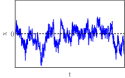
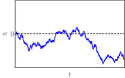
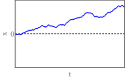
Figure 1: Stochastic realizations of one-sided MvN fBm $x(t)$ for $H=1/4$ (top left) and $H=3/4$ (bottom). $H=1/2$ (top right) corresponds to the standard Bm.

General expressions and main results. – Quite generally, the action functional $S[X(t)]$ of a Gaussian process $X(t)$ on a time interval $\Omega$ can be represented as zinn

$$S[X(t)]=\frac{1}{2}\int_{\Omega}dt_{1}\int_{\Omega}dt_{2}\,\mathcal{K}(t_{1},t_{2})\,X(t_{1})\,X(t_{2})\,.$$ (4)

The kernel $\mathcal{K}(t_{1},t_{2})$ (a symmetric function of $t_{1}$ and $t_{2}$) is the inverse of the covariance function $\kappa(t_{1},t_{2})$ of the process $X(t)$:

$$\int_{\Omega}dt_{1}\,\kappa\left(t_{1},t_{3}\right)\,\mathcal{K}(t_{1},t_{2})=\delta\left(t_{2}-t_{3}\right)\,.$$ (5)

Once $\mathcal{K}(t_{1},t_{2})$ is known, the action functional (4) is completely defined, giving the probability density $P[X(t)]$ of a given realization of the process $X(t)$. Now we present our main results for the action functionals of the MvN fBm $x(t)$. They have different forms for the sub-diffusive and super-diffusive fBm, and for the two- and one-sided processes.

We start with the sub-diffusion. For the two-sided sub-diffusive ($0<H<1/2$) fBm $x(t)$, the action $S=S[x(t)]$ is given by

$$S=\frac{{\rm cot}(\pi H)}{4\pi H}\int^{\infty}_{-\infty}\int^{\infty}_{-\infty}\frac{dt_{1}dt_{2}}{|t_{1}-t_{2}|^{2H}}\,\dot{x}(t_{1})\dot{x}(t_{2})\,.$$ (6)

For the one-sided sub-diffusive fBm we obtain

$$S\!=\!\frac{{\rm cot}(\pi H)}{4\pi H}\!\int^{\infty}_{0}\int^{\infty}_{0}\!\!\frac{dt_{1}dt_{2}\,I_{z}\left(\frac{1}{2}-H,H\right)}{|t_{1}-t_{2}|^{2H}}\dot{x}(t_{1})\dot{x}(t_{2}),$$ (7)

where $I_{z}(a,b)$ is the regularized incomplete beta function

$$I_{z}(a,b)=\frac{\Gamma(a+b)}{\Gamma(a)\Gamma(b)}\int^{z}_{0}x^{a-1}(1-x)^{b-1}dx\,,$$ (8)

$\Gamma(\dots)$ is the gamma function, and $z=4t_{1}t_{2}(t_{1}+t_{2})^{-2}$.

As one can see, the action functionals (6) and (7) are non-local in time and written in terms of the fGn $\dot{x}(t)$, rather than in terms of $x(t)$ itself. The expression (7) for the one-sided case is more complicated, than that for the two-sided one, Eq. (6). In particular, the two-sided kernel in Eq. (6) is a difference kernel, which reflects the stationarity in time of the two-sided derivative process, the fGn. The one-sided kernel (7) is not a difference kernel in spite of the stationarity of the fGn. The non-stationarity, however, is temporary, as it is caused by a transient created by the initial condition $x(t=0)=0$. Indeed, in the limit of $t_{1},t_{2}\to\infty$, and $t_{1}-t_{2}=\text{const}$, $z$ tends to $1$, the one-sided kernel coincides with the two-sided one, and the stationarity is restored.

In the limiting case $H=1/2$, the kernels in Eqs. (6) and (7) become delta-functions and yield the classical Wiener’s formula (1), as we show in Ref. SM .

For $H=1/4$ Eq. (6) has the same functional form as the two-sided expression (3), as to be expected in view of the pre-thermalization of the Rouse polymer bead . We also remark that Eq. (6) was postulated in Ref. nech as an effective Hamiltonian of topologically stabilized polymers in melts, permitting to cover various conformations ranging from ideal Gaussian coils to crumpled globules. Our derivation validates their approach.

Now we present our results for the super-diffusive fBm, $1/2<H<1$. In the two-sided case we obtain

$$S\!=\!\frac{\sigma(H)}{2}\,\!\int^{\infty}_{-\infty}\!\int^{\infty}_{-\infty}dt_{1}\,dt_{2}\,|t_{1}-t_{2}|^{2-2H}\,\ddot{x}(t_{1})\,\ddot{x}(t_{2})\,,$$ (9)

where

$$\sigma(H)=-\frac{{\rm cot}(\pi H)}{4\pi H(1-H)(2H-1)}\,,$$ (10)

a positive function. For the one-sided case

$$S = \frac{\sigma(H)}{2}\,\int^{\infty}_{0}\int^{\infty}_{0}dt_{1}\,dt_{2}\,|t_{1}-t_{2}|^{2-2H}$$ (11)

$$\times I_{z^{\prime}}\left(\frac{3}{2}-H,2H-2\right)\ddot{x}(t_{1})\ddot{x}(t_{2})\,,$$

where $z^{\prime}={\rm min}(t_{1},t_{2})/{\rm max}(t_{1},t_{2})$. Again, the expressions in Eqs. (9) and (11) are non-local in time, but now they are written in terms of $\ddot{x}(t)$, that is in terms of the first derivative of the fGn. The two-sided kernel is a difference kernel. The one-sided kernel is not, but it approaches the difference form following an initial transient. Also, the classical Wiener’s form (1) is recovered in the limit $H\to 1/2$ SM .

Expressions (6)-(11), alongside with Eqs. (25) and (27) below, represent the main results of this work. Here we present derivations of Eqs. (6) and (9) for the two-sided sub-diffusive and super-diffusive fBm, respectively. The derivation of the (a bit more bulky) one-sided expressions in Eqs. (7) and (11) is relegated to the SM SM .

Sub-diffusion – Here we work directly with the fGn. Its covariance function $c(t_{1},t_{2})$ can be readily calculated:

$$c(t_{1},t_{2})=\langle y(t_{1})y(t_{2})\rangle=\langle\dot{x}(t_{1})\dot{x}(t_{2})\rangle$$

$$=\frac{\partial^{2}}{\partial t_{1}\partial t_{2}}\langle x(t_{1})x(t_{2})\rangle=\frac{d}{d\tau}\left(H|\tau|^{2H-1}\text{sgn}\,\tau\right)\,,$$ (12)

where $\tau=t_{1}-t_{2}$, and we used Eq. (2). Equation (12) holds both for the two-sided and the one-sided process and for all $0<H<1$. Notably, the fGn is a stationary process. For $H=1/2$ Eq. (12) gives $c(\tau)=(1/2)(d/d\tau)\,\text{sgn}\,\tau=\delta(\tau)$, as to be expected for the white noise.

Let us denote by $\mathcal{C}(\tau)$ the kernel inverse to $c(\tau)$. For the two-sided process, $\mathcal{C}(\tau)$ is defined by the equation $\int_{-\infty}^{\infty}d\tau\,c\left(\tau-t\right)\,\mathcal{C}(\tau)=\delta(t)$ or, in the explicit form,

$$\int_{-\infty}^{\infty}d\tau\,\mathcal{C}(\tau)\frac{d}{d\tau}\left[|\tau-t|^{2H-1}\text{sgn}(\tau-t)\right]=\frac{1}{H}\,\delta(t).$$ (13)

Integrating by part and assuming that the boundary terms are zero (as can be verified a posteriori), we arrive at the integral equation

$$\int_{-\infty}^{\infty}d\tau\,\frac{\text{sgn}(\tau-t)}{|\tau-t|^{1-2H}}\,\mathcal{D}(\tau)=-\frac{1}{H}\,\delta(t)$$ (14)

for the unknown function $\mathcal{D}(\tau)=d\mathcal{C}(\tau)/d\tau$. The solution can be found in Ref. kilbas :

$$\mathcal{D}(\tau)=\frac{d\mathcal{C}(\tau)}{d\tau}=\frac{\text{cot}\,(\pi H)}{2\pi H}\frac{d}{d\tau}\frac{1}{|\tau|^{2H}}\,.$$ (15)

Getting rid of the $\tau$-derivative and using the fact that the kernel must vanish at $|\tau|\to\infty$, we obtain

$$\mathcal{C}(\tau)=\frac{\text{cot}\,(\pi H)}{2\pi H}\frac{1}{|\tau|^{2H}}\,.$$ (16)

The ensuing Gaussian action functional (4), written in terms of $X(t)=\dot{x}(t)$, yields the announced equation (6).

Super-diffusion – Here we work with the second-derivative process $z(t)=\ddot{x}(t)$. Its covariance is

$$q(t_{1},t_{2})=\frac{d^{3}}{d\tau^{3}}\left[H|\tau|^{2H-1}\text{sgn}(\tau)\right]\,.$$ (17)

For the two-sided process the inverse kernel $\mathcal{Q}(t_{1},t_{2})$ is defied by the equation $\int_{-\infty}^{\infty}d\tau\,q\left(\tau-t\right)\,\mathcal{Q}(\tau)=\delta(t)$, or, in the explicit form,

$$\int_{-\infty}^{\infty}d\tau\,\mathcal{Q}(\tau)\frac{d^{3}}{d\tau^{3}}\left[|\tau-t|^{2H-1}\text{sgn}(\tau-t)\right]=\frac{1}{H}\,\delta(t).$$ (18)

Integrating three times by part and assuming that the boundary terms are zero (as verified a posteriori), we arrive at the equation

$$\int_{-\infty}^{\infty}d\tau\,\frac{\text{sgn}(\tau-t)}{|\tau-t|^{1-2H}}\,\mathcal{Z}(\tau)=-\frac{1}{H}\,\delta(t),$$ (19)

where $\mathcal{Z}(\tau)=d^{3}\mathcal{Q}(\tau)/d\tau^{3}$. This is exactly the same equation as Eq. (14), but now $1-2H<0$. It is convenient to rewrite this equation as

$$-\int_{-\infty}^{t}d\tau\,\left(t-\tau\right)^{2H-1}\mathcal{Z}(\tau) + \int_{t}^{\infty}d\tau\,\left(\tau-t\right)^{2H-1}\mathcal{Z}(\tau)$$ (20)

$$= -\frac{1}{H}\,\delta(t)$$

and differentiate both sides of Eq. (20) with respect to $t$. The resulting equation,

$$\int_{-\infty}^{\infty}d\tau\,\frac{\mathcal{Z}(\tau)}{|\tau-t|^{2-2H}}=\frac{1}{H(2H-1)}\,\delta^{\prime}(t),$$ (21)

is solvable kilbas , and we obtain

$$\mathcal{Z}(\tau)=-\frac{\text{cot}(\pi H)}{2\pi H(2H-1)}\,\frac{d^{2}}{d\tau^{2}}\frac{\text{sgn}\,\tau}{|\tau|^{2H-1}}\,.$$ (22)

Integrating this expression over $\tau$ three times and using account the fact that the kernel must vanish at $|\tau|\to\infty$, we obtain the desired inverse kernel:

$$\mathcal{Q}(\tau)=\sigma(H)\,|\tau|^{2(1-H)}\,,$$ (23)

where $\sigma(H)$ is defined in Eq. (10). The resulting Gaussian action functional (4), written in terms of $X(t)=z(t)\equiv\ddot{x}(t)$, yields the announced Eq. (9).

External force – An important extension of this formalism deals with situations where the fBm of a particle is accompanied by its overdamped motion under external force $f(x)$. A natural approach to modelling this situation employs the non-Markovian Langevin equation Metzler2021

$$\dot{x}(t)=f[x(t)]+y(t)\,,$$ (24)

where the noise term $y(t)$ describes fGn. When the external force $f(x)$ is confining, the $x$-distribution approaches a steady state. This steady state, however, is non-Boltzmann. Therefore, not surprisingly, it violates the fluctuation-dissipation theorem Metzler2021 . As the fGn $y(t)$ is a Gaussian process, a natural path-integral representation for Eq. (24) is provided by the action functional

$$S[x(t)] = \frac{1}{2}\int_{-\infty}^{\infty}dt_{1}\int_{-\infty}^{\infty}dt_{2}\,\mathcal{C}(t_{1}-t_{2})\,\{\dot{x}(t_{1})-f[x(t_{1})]\}$$ (25)

$$\times \{\dot{x}(t_{2})-f[x(t_{2})]\}\,,$$

where $\mathcal{C}(\tau)$ is the inverse kernel for the fGn, given by Eq. (16). Here we assumed a two-sided sub-diffusive fBm.

For a super-diffusive fBm a suitable non-Markovian Langevin equation can be obtained by a formal differentiation of Eq. (24) with respect to time, leading to

$$\ddot{x}(t)=f^{\prime}[x(t)]\dot{x}(t)+z(t)\,,$$ (26)

where $f^{\prime}(x)\equiv df(x)/dx$, and the noise term $z(t)$ is the time derivative of the fGn. The corresponding path integral for the two-sided process is given by the action functional

$$S[x(t)]=\frac{1}{2}\int_{-\infty}^{\infty}dt_{1}\int_{-\infty}^{\infty}dt_{2}\,\mathcal{Q}(t_{1}-t_{2})$$ (27)

$$\times \!\!\left[\ddot{x}(t_{1})-f^{\prime}[x(t_{1})]\,\dot{x}(t_{1})\right]\left[\ddot{x}(t_{2})-f^{\prime}[x(t_{2})]\,\dot{x}(t_{2})\right],$$

where $\mathcal{Q}(\tau)$ is given by Eq. (23). Expressions similar to Eqs. (25) and (27), but with the one-side kernels as in Eqs. (7) and (11), hold for the one-sided sub- and super-diffusive fBm, respectively.

Summary. – We generalized the classical Wiener’s path integral for the Bm and found exact path-integral representations for the two-sided and one-sided MvN fBm for the whole range $0<H<1$ of the Hurst exponent. We also extended the formalism to include external forcing. The exact and explicit path-integral representations open new inroads into analytical and numerical studies of fBm – an important paradigm of scale-invariant stochastic processes with memory – in a multitude of applications in natural sciences, technology and finance.

Acknowledgments. – We are grateful to P. Chigansky, D. S. Dean, S. N. Majumdar and K. L. Sebastian for useful discussions. B. M. was supported by the Israel Science Foundation (Grant No. 1499/20).

Appendix A Supplemental Material

Here we present some details of derivations of the results obtained for the one-sided case and also show that in the limit $H\to 1/2$ the expressions (6), (7), (9) and (11) converge to the Wiener result in Eq. (1).

Appendix B Two-sided fBm

B.1 Sub-diffusion, $0<H<1/2$. The limit of $H\to 1/2$

In order to take the limit $H\to 1/2$, we take advantage of the identity

$$\frac{1}{|t_{1}-t_{2}|^{2H}}=\frac{1}{(1-2H)}\frac{d}{dt_{1}}\frac{{\rm sgn}(t_{1}-t_{2})}{|t_{1}-t_{2}|^{2H-1}}\,,$$ (S1)

which permits us to formally rewrite the kernel in Eq. (3) as

$$\frac{{\rm cot}(\pi H)}{2\pi H}\frac{1}{|t_{1}-t_{2}|^{2H}}=\frac{{\rm cot}(\pi H)}{2\pi H(1-2H)}\frac{d}{dt_{1}}\frac{{\rm sgn}(t_{1}-t_{2})}{|t_{1}-t_{2}|^{2H-1}}\,.$$ (S2)

Taking the limit $H\to 1/2$ in the both sides of the latter equality and noticing that

$$\lim_{H\to 1/2}\frac{{\rm cot}(\pi H)}{(1-2H)}=\frac{\pi}{2}\,,$$ (S3)

we get

$$\lim_{H\to 1/2}\frac{{\rm cot}(\pi H)}{2\pi H}\frac{1}{|t_{1}-t_{2}|^{2H}} =\lim_{H\to 1/2}\frac{{\rm cot}(\pi H)}{2\pi H(1-2H)}\frac{d}{dt_{1}}\frac{{\rm sgn}(t_{1}-t_{2})}{|t_{1}-t_{2}|^{2H-1}}$$ (S4)

$$=\frac{1}{2}\frac{d}{dt_{1}}{\rm sgn}(t_{1}-t_{2})=\delta(t_{1}-t_{2})\,,$$ (S5)

which yields the Wiener expression (1).

B.2 Super-diffusion, $1/2<H<1$. The limit of $H\to 1/2$

We turn to the limit $H\to 1/2$ directly in Eq. (22) in the main text to get

$$\lim_{H\to 1/2}\mathcal{Z}(\tau)=\mathcal{Z}_{H=1/2}(\tau)=\frac{1}{2}\frac{d^{2}}{d\tau^{2}}{\rm sgn}(\tau)=\frac{d}{d\tau}\delta(\tau)$$ (S6)

The action $S$ written in terms of the derivative of the fractional Gaussian noise involves the kernel function $\mathcal{Q}$, which is given by a triple integral of $\mathcal{Z}_{H=1/2}(\tau)$ [see Eq. (23)]. Consequently, the action has the form

$$S=\frac{1}{2}\int^{\infty}_{-\infty}\int^{\infty}_{-\infty}dt_{1}dt_{2}\ddot{x}(t_{1})\ddot{x}(t_{2})\int^{t_{1}}_{-\infty}\int^{t_{2}}_{-\infty}d\tau_{1}d\tau_{2}\delta(\tau_{1}-\tau_{2})\,.$$ (S7)

Integrating the latter expression by parts, we arrive at the Wiener’s result in Eq. (1).

Appendix C One-sided fBm

Here we present brief derivations of our expressions (7) and (11) of the main text.

C.1 Sub-diffusion, $0<H<1/2$

For the one-sided sub-diffusive fBm the inverse kernel $\mathcal{C}(t_{1},t_{2})$ is not a difference kernel, and Eq. (13) gives way to the equation

$$\int_{0}^{\infty}dt_{1}\,\mathcal{C}(t_{1},t_{2})\frac{d}{dt_{1}}\left[|t_{1}-t_{3}|^{2H-1}\text{sgn}(t_{1}-t_{3})\right]=\frac{1}{H}\,\delta(t_{2}-t_{3})\,.$$ (S8)

Integrating by part, we arrive at

$$\int_{0}^{\infty}dt_{1}\,\frac{\text{sgn}(t_{1}-t_{3})}{|t_{1}-t_{3}|^{1-2H}}\,\mathcal{D}(t_{1},t_{2})=-\frac{1}{H}\,\delta(t_{2}-t_{3}),$$ (S9)

where $\mathcal{D}(t_{1},t_{2})=(\partial/\partial t_{1})\,\mathcal{C}(t_{1},t_{2})$. The solution can be found in Ref. [47]. Getting rid of the $t_{1}$-derivative, we obtain $\mathcal{C}(t_{1},t_{2})$ in the following three alternative (but equivalent) forms

$$\mathcal{C}(t_{1},t_{2}) =\frac{(t_{1}t_{2})^{-H}\sqrt{z^{\prime}}}{H(1-2H)\sin(\pi H)\Gamma(2H)\Gamma^{2}\left(\frac{1}{2}-H\right)}\,_{2}F_{1}\left(1,H+\frac{1}{2};\frac{3}{2}-H;z^{\prime}\right)\,,\quad z^{\prime}=\frac{{\rm min}(t_{1},t_{2})}{{\rm max}(t_{1},t_{2})}$$ (S10)

$$=\frac{{\rm cot}(\pi H)(t_{1}t_{2})^{-H}\sqrt{z}}{2\pi H(1-2H)B(1/2-H,2H)}\,_{2}F_{1}\left(\frac{1}{2},1;\frac{3}{2}-H;z\right)\,,\quad z=\frac{4t_{1}t_{2}}{(t_{1}+t_{2})^{2}}$$ (S11)

$$=\frac{{\rm cot}(\pi H)}{2\sqrt{\pi}\Gamma(1/2-H)\Gamma(1+H)}\frac{B_{z}(1/2-H,H)}{|t_{1}-t_{2}|^{2H}}\,,$$ (S12)

where $B(a,b)$ and $B_{z}(a,b)$ are the complete and incomplete beta-functions, respectively, and ${}_{2}F_{1}(\dots)$ is the hypergeometric function. Recalling next the definition of the regularized incomplete beta-function [see Eq. (8)], we obtain our result in Eq. (7).

Limit $H\to 1/2$. To take the limit $H\to 1/2$ in Eq. (7) in the main text it is expedient to use the representations of the kernel $\mathcal{C}(t_{1},t_{2})$ given in the second line in Eq. (S10). We formally rewrite the Gauss hypergeometric function entering this representation as

$$\,{}_{2}F_{1}\left(\frac{1}{2},1;\frac{3}{2}-H;z\right)=\frac{\Gamma(H)\Gamma(3/2-H)}{\sqrt{\pi}(1-z)^{H}z^{1/2-H}}-\frac{(1/2-H)}{H}\,_{2}F_{1}\left(\frac{1}{2},1;1+H;1-z\right)$$ (S13)

such that, after some algebra, the kernel $\mathcal{C}(t_{1},t_{2})$ can be cast into the form

$$\mathcal{C}(t_{1},t_{2})=\frac{{\rm cot}(\pi H)}{2\pi H}\frac{1}{|t_{1}-t_{2}|^{2H}}-\frac{{\rm cot}(\pi H)}{2\pi H^{2}B(1/2-H,2H)}\frac{(t_{1}t_{2})^{1/2-H}}{(t_{1}+t_{2})}\,_{2}F_{1}\left(\frac{1}{2},1;1+H;\left(\frac{t_{1}-t_{2}}{t_{1}+t_{2}}\right)^{2}\right)$$ (S14)

Further on, we observe that the numerical $H$-dependent amplitude in the second term in the latter expression vanishes in the limit $H\to 1/2$ as

$$\frac{{\rm cot}(\pi H)}{2\pi H^{2}B(1/2-H,2H)}\simeq 2\left(\frac{1}{2}-H\right)^{2}\,,$$ (S15)

which signifies that this term does not contribute in this limit. On the contrary, as demonstrated above, the first term converges to the delta-function which ensures that the action in Eq. (7) in the main text converges to the Wiener’s result in Eq. (1).

C.2 Super-diffusion, $1/2<H<1$

Here we present a derivation of Eq. (11) and also check the limit of $H\to 1/2$. In particular, this derivation highlights the reason why the representation of the action in terms of $\ddot{x}$ is advantageous.

We start the derivation by representing the action in terms of the first derivative of the fBm, that is in terms of the fGn:

$$S=\frac{1}{2}\int^{\infty}_{0}\int^{\infty}_{0}dt_{1}dt_{2}\mathcal{C}(t_{1},t_{2})\dot{x}(t_{1})\dot{x}(t_{2})\,.$$ (S16)

The inverse kernel $\mathcal{C}(t_{1},t_{2})$ obeys the integral equation

$$\int^{\infty}_{0}\frac{dt_{1}\,\mathcal{C}(t_{1},t_{2})}{|t_{1}-t_{3}|^{2-2H}}=\frac{\delta(t_{2}-t_{3})}{H(2H-1)}\,.$$ (S17)

The explicit solution of this equation can be found in Ref. Lundgren . After straightforward transformations, it reads:

$$\mathcal{C}(t_{1},t_{2}) =\frac{1}{2H\sin(\pi H)\Gamma(2H)\Gamma^{2}(3/2-H)}\frac{d^{2}}{dt_{1}dt_{2}}\int_{0}^{{\rm min}(t_{1},t_{2})}\frac{d\tau}{(t_{1}-\tau)^{H-1/2}(t_{2}-\tau)^{H-1/2}}$$ (S18)

$$=\frac{1}{2H\sin(\pi H)\Gamma(2H)\Gamma^{2}(3/2-H)}\frac{d^{2}}{dt_{1}dt_{2}}|t_{1}-t_{2}|^{2-2H}B_{z^{\prime}}(3/2-H,2H-2)\,,\quad z^{\prime}=\frac{{\rm min}(t_{1},t_{2})}{{\rm max}(t_{1},t_{2})}\,.$$ (S19)

We observe that the function $\mathcal{C}(t_{1},t_{2})$, defined in the right-hand-side of Eq. (S18), contains a non-integrable singularity at $t_{1}=t_{2}$, which shows why the representation of the action in Eq. (S16) in terms of the first derivatives $\dot{x}(t)$ is problematic. To get a regular result, we integrate Eq. (S16) by part, i.e. express it in terms of the second derivatives $\ddot{x}(t_{1})$ and $\ddot{x}(t_{2})$. Then, using the definition of the regularized incomplete beta-function in Eq. (8), we arrive at the final result in Eq. (11).

Limit $H\to 1/2$. The limit $H\to 1/2$ can be conveniently taken in the expression given in the first line of Eq. (S18). This yields

$$\lim_{H\to 1/2}\mathcal{C}(t_{1},t_{2})=\frac{d^{2}}{dt_{1}dt_{2}}{\rm min}(t_{1},t_{2})=\delta(t_{1}-t_{2})\,,$$ (S20)

and we recover the Wiener’s expression in Eq. (1).

References

- (1) N. Wiener, Proc. Natl. Acad. Sci. USA 7, 253 (1921); Proc. Natl. Acad. Sci. USA 7, 294 (1921); J. Math. Phys. Sci. 2, 132 (1923); Proc. London Math. Soc. 22, 454 (1924); Acta Math. 55, 117 (1930).
- (2) M. Kac, Trans. Amer. Math. Soc. 65, 1 (1949).
- (3) S. N. Majumdar, Curr. Sci. 89, 2076 (2005).
- (4) A. J. Bray, S. N. Majumdar, and G. Schehr, Adv. Phys. 62, 225 (2013).
- (5) V. Démery and D. S. Dean, Phys. Rev. E 84, 011148 (2011).
- (6) D. S. Dean and R. Horgan, Phys. Rev. E 76, 041102 (2007).
- (7) R. P. Feynman, Rev. Mod. Phys. 20, 367 (1948).
- (8) R. P. Feynman and A. R. Hibbs, Quantum Mechanics and Path Integrals (McGraw-Hill, New York, 1965).
- (9) Feynman’s Thesis – A New Approach to Quantum Theory, edited by L. M. Brown (World Scientific, Singapor, 2005).
- (10) L. S. Schulman, Techniques and Applications of Path Integration (Wiley, New York, 1981).
- (11) F.W. Wiegel, Introduction to Path-Integral Methods in Physics and Polymer Science, (World Scientific, Philadelphia, 1986).
- (12) M. Chaichian and A. P. Demichev, Stochastic Processes and Quantum Mechanics (Path Integrals in Physics., vol. 1.) (Institute of Physics Publishing, Bristol, 2001).
- (13) J. Zinn-Justin. Quantum Field Theory and Critical Phenomena (International Series of Monographs on Physics, vol. 113) (Clarendon, Oxford, 2002).
- (14) H. Kleinert, Path Integrals in Quantum Mechanics, Statistics, Polymer Physics, and Financial Markets (World Scientific, Singapore, 2009).
- (15) A. Kamenev, Field Theory of Non-Equilibrium Systems (Cambridge University Press, Cambridge, UK, 2011).
- (16) H. S. Wio, Path Integrals for Stochastic Processes. An Introduction (World Scientific, Singapore, 2013).
- (17) L. F. Cugliandolo, V. Lecomte, and F. van Wijland, J. Phys. A: Math. Theor. 52 50LT01 (2019).
- (18) B. B. Mandelbrot and J. W. van Ness, SIAM Review 10, 422 (1968).
- (19) A. N. Kolmogorov, CR (Dokl.) Acad. Sci. URSS 26, 115 (1940).
- (20) A.-L. Barabási and H. E. Stanley, Fractal Concepts in Surface Growth (Cambridge University Press, Cambridge, England, 1995).
- (21) J. Krug, H. Kallabis, S. N. Majumdar, S. J. Cornell, A. J. Bray,and C. Sire, Phys. Rev. E 56, 2702 (1997).
- (22) M. Weiss, Phys. Rev. E 88, 010101(R) (2013).
- (23) D. Ernst, M. Hellmann, J. Köhler, and M. Weiss, Soft Matter 8, 4886 (2012).
- (24) S. C. Weber, A. J. Spakowitz, and J. A. Theriot, Phys. Rev. Lett. 104, 238102 (2010).
- (25) I. Bronshtein, E. Kepten, I. Kanter, S. Berezin, M. Lindner, A. B. Redwood, S. Mai, S. Gonzalo, R. Foisner, Y. Shav-Tal, and Y. Garini, Nat. Commun. 6, 8044 (2015).
- (26) D. Krapf, N. Lukat, E. Marinari, R. Metzler, G. Oshanin, C. Selhuber-Unkel, A. Squarcini, L. Stadler, M. Weiss, and X. Xu, Phys. Rev. X 9, 011019 (2019).
- (27) S. Janusonis, N. Detering, R. Metzler, and T. Vojta, Frontiers Comp. Neurosci. 14, 56 (2020).
- (28) J.-C. Walter, A. Ferrantini, E. Carlon, and C. Vanderzande, Phys. Rev. E 85, 031120 (2012).
- (29) A. Amitai, Y. Kantor, and M. Kardar, Phys. Rev. E 81, 011107 (2010).
- (30) A. Zoia, A. Rosso, and S. N. Majumdar, Phys. Rev. Lett. 102, 120602 (2009).
- (31) J. L. A. Dubbeldam, V. G. Rostiashvili, A. Milchev, and T. A. Vilgis, Phys. Rev. E 83, 011802 (2011).
- (32) V. Palyulin, T. Ala-Nissila, and R. Metzler, Soft Matter 10, 9016 (2014).
- (33) V. Kukla, J. Kornatowski, D. Demuth, I. Girnus, H. Pfeifer, L. V. C. Rees, S. Schunk, K. K. Unger, and J. K¨arger, Science 272, 702 (1996).
- (34) Q.-H. Wei, C. Bechinger, and P. Leiderer, Science 287, 625 (2000).
- (35) O. Bénichou, P. Illian, G. Oshanin, A. Sarracino, and R. Voituriez, J. Phys.: Condens. Matter 30, 443001 (2018).
- (36) R. Metzler, J.-H. Jeon, A. G. Cherstvy, and E. Barkai, Phys. Chem. Chem. Phys. 16, 24128 (2014).
- (37) F. J. Molz, H. H. Liu, and J. Szulga, Water Resources Res. 33, 2273 (1997).
- (38) R.J. Barton and H.V. Poor, IEEE Trans. Inform. Theory 34, 943 (1988).
- (39) E. Myrvoll-Nilsen, H.-B. Fredriksen, S. H. Sørbye, and M. Rypdal, Front. Earth Sci. 7, 214 (2019).
- (40) V. Maxim, L. Sendur, J. Fadili, J. Suckling, R. Gould, R. Howard, and E. Bullmore, Neuroimage 25, 141 (2005).
- (41) In simple large-deviation problems, analyzed with the optimal fluctuation method, the explicit knowledge of the inverse kernel can be unnecessary. This happens when the ensuing nonlocal Euler-Lagrange equation (a linear integral equation) can be transformed into a form containing only the covariance function of the process baruch ; longtimeLD ; escape . For more complicated problems, however, no such transformation exists, and the knowledge of the inverse kernel is indispensable.
- (42) For the Riemann-Liouville fBm (a different mathematical model of anomalous diffusion, introduced by Levy Levy ), the action can be determined by employing fractional calculus, as was done in Refs. seb ; san and in Chapter 10 in Ref. book4 . Also, in Refs. Calvo ; Wiopaper a path-integral representation was found for the fractional Levy motion Calvo , still another mathematical model. All these results, however, are irrelevant to the MvN fBm studied in our work.
- (43) S. F. Burlatskii and G. Oshanin, Theor. Math. Phys. 75(3), 659 (1988).
- (44) K. Polovnikov, S. Nechaev, and M. V. Tamm, Soft Matter 14, 6561 (2018).
- (45) K. J. Wiese, S. N. Majumdar, and A. Rosso, Phys. Rev. E 83, 061141 (2011).
- (46) M. Delorme and K. J. Wiese, Phys. Rev. Lett. 115, 210601 (2015).
- (47) M. Delorme and K. J. Wiese, Phys. Rev. E 94, 012134 (2016).
- (48) M. Delorme and K. J. Wiese, Phys. Rev. E 94, 052105 (2016).
- (49) T. Sadhu, M. Delorme and K. J. Wiese, Phys. Rev. Lett. 120, 040603 (2018).
- (50) S. M. J. Khadem, R. Klages and S. H. L. Klapp, arXiv:2205.15791.
- (51) Indeed, although is a Gaussian process, the Wiener’s action (1) is expressed through , rather than through . Furthermore, one can rewrite Eq. (1) as , with a delta-function kernel. In the -representation the kernel, , is more singular and less convenient to work with.
- (52) S. G. Samko, A. A. Kilbas and A. I. Marichev, Fractional integrals and derivatives: Theory and Applications, (Gordon and Breach, Paris, 1993).
- (53) A. D. Polyanin and A. V. Manzhirov, Handbook of Integral Equations (Taylor & Francis Group, Boca Raton, FL, USA, 2008).
- (54) See Supplemental Material at … for some derivations and technical details.
- (55) T. Guggenberger, A. Chechkin, and R. Metzler, J. Phys. A: Math. Theor. 54, 29 (2021).
- (56) B. Meerson and G. Oshanin, Phys. Rev. E 105, 064137 (2022).
- (57) B. Meerson, Phys. Rev. E 100, 042135 (2019).
- (58) B. Meerson, Phys. Rev. E 105, 034106 (2022).
- (59) P. Lévy, University of California Publications in Statistics 1, 331 (1953).
- (60) K. L. Sebastian, J. Phys. A: Math. Gen. 28, 4305 (1995).
- (61) I. Calvo and R. Sanchez, J. Phys. A: Math. Theor. 41, 282002 (2008).
- (62) I. Calvo, R. Sánchez and B. A. Carreras, J. Phys. A: Math. Theor. 42, 055003 (2009).
- (63) H. S. Wio, J. Phys. A: Math. Theor. 46, 115005 (2013).
- (64) T. Lundgren and D. Chiang, Quart. Appl. Math. 24, 303 (1967).