Logarithmic entanglement scaling in dissipative free-fermion systems

Abstract

We study the quantum information spreading in one-dimensional free-fermion systems in the presence of localized thermal baths. We employ a nonlocal Lindblad master equation to describe the system-bath interaction, in the sense that the Lindblad operators are written in terms of the Bogoliubov operators of the closed system, and hence are nonlocal in space. The statistical ensemble describing the steady state is written in terms of a convex combination of the Fermi-Dirac distributions of the baths. Due to the singularity of the free-fermion dispersion, the steady-state mutual information exhibits singularities as a function of the system parameters. While the mutual information generically satisfies an area law, at the singular points it exhibits logarithmic scaling as a function of subsystem size. By employing the Fisher-Hartwig theorem, we derive the prefactor of the logarithmic scaling, which depends on the parameters of the baths and plays the role of an effective “central charge”. This is upper bounded by the central charge governing ground-state entanglement scaling. We provide numerical checks of our results in the paradigmatic tight-binding chain and the Kitaev chain.

I Introduction

The study of the interplay between the microscopic quantum world and the macroscopic classical one is a fundamental research topic in contemporary physics, although it dates back to the first days of quantum mechanics [1, 2]. Typically, the interaction with the environment is believed to destroy genuine quantum behaviors, although consensus is emerging that this is not always the case. Dissipation-based protocols have been devised to imprint nontrivial correlations in quantum many-body systems (see, e.g., Refs. [3, 4, 5, 6, 7, 8, 9, 10, 11, 12]). A first crucial question is whether entanglement, which is the distinctive feature of quantum mechanics, is robust against the presence of the environment. Second, is it possible to enhance the entanglement content of a quantum many-body state via an ad hoc engineered environment? Answering these questions is a daunting task, because there is no universal approach (neither analytic nor numerical) to tackle generic open quantum many-body systems. With this state of affairs, one has to resort to approximate treatments. Markovian master equations, such as the Lindblad master equation [13, 14, 15], provide some of the most successful tools to attack open quantum many-body systems.

Particularly important settings are provided by the class of nonequilibrium boundary-driven quantum systems, which have been the subject of intense research in recent years (see, e.g., Refs. [16, 17] and references therein). In this paper we focus on the one-dimensional setup illustrated in Fig. 1: a system of noninteracting fermions is locally coupled to ideal thermal baths. To be specific, we focus on the tight-binding chain and on the Kitaev chain. The fermions live on a lattice with $N$ sites, with either periodic boundary conditions (PBC) or open boundary conditions (OBC). The system is put in contact with two ideal fermionic reservoirs at temperatures $T_{L},T_{R}$, and with chemical potentials $\mu_{L},\mu_{R}$. With OBC the two baths are placed at the edges of the chain [Fig. 1(a)], whereas with PBC they are are at the maximum distance $N/2$ [Fig. 1(b)]. The interaction between the chain and the reservoirs is treated within the formalism of the Lindblad master equation [15]. Specifically, we employ the nonlocal description derived in Ref. [18]. The Lindblad operators are obtained ab initio from the microscopic system-bath interaction, and are written in terms of the Bogoliubov modes of the model without dissipation. As such, the Lindblad operators are non-local in real space. Interestingly, this allows to recover the Conformal Field Theory (CFT) description of the chain in the low-temperature limit. Furthermore, the nonlocal Lindblad approach allows to obtain a thermodynamically consistent description of transport properties [18, 19].

We are interested in the quantum correlations emerging in the steady state of finite chains of length $N$, in the limit $t\to\infty$. The ensemble describing this state is written in terms of a convex combination of the Fermi-Dirac distributions of the reservoirs [18]. Importantly, this ensemble is in general different from the finite-temperature ensemble of the underlying fermionic chain. In particular, we will show that ground-state criticality of the free chain Hamiltonian is associated with nontrivial steady-state correlations in the dissipative model. To monitor these correlations, we consider the quantum mutual information $I(A_{1}:A_{2})$ between two subregions $A_{1}$ and $A_{2}$ of the chain, defined as [20, 21, 22, 23]

$$I(A_{1}:A_{2})\coloneqq S_{A_{1}}+S_{A_{2}}-S_{A_{1}\cup A_{2}},$$ (1)

where $S_{A}$ is the von Neumann entropy of the subregion $A$, which is defined as

$$S_{A}\coloneqq-\Tr[\rho_{A}\ln\rho_{A}],$$ (2)

where $\rho_{A}$ is the reduced density matrix for subsystem $A$.

For pure states the von Neumann entropy $S_{A}$ of a subsystem quantifies its entanglement with the rest of the system. Moreover, one has that $S_{A}=S_{\overline{A}}$, with $\overline{A}$ being the complement of $A$ [see, for instance, Fig. 1(a)], and $S_{A\cup\overline{A}}=0$. However, in the presence of an environment, the global state is mixed, which implies that neither the von Neumann entropy nor the mutual information are proper measures of the entanglement shared between different regions. Still, it has been shown recently that for out-of-equilibrium free-fermion and free-boson models in the presence of quadratic global dissipation the mutual information admits a hydrodynamic description in terms of a quasiparticle picture [24, 25, 26, 27]. Moreover, we numerically checked that our findings remain qualitatively valid using the fermionic entanglement negativity, which, on the other hand, is a proper measure of entanglement [28, 29].

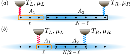
Figure 1: The setup used in this work. A one-dimensional chain of $N$ noninteracting fermions is put in contact with two thermal reservoirs at temperatures $T_{L}$, $T_{R}$ and chemical potentials $\mu_{L}$, $\mu_{R}$. (a) In the case of OBC, only the sites at the edges are in contact with the baths, and we are interested in the steady-state mutual information $I(A_{1}:A_{2})$ between the two connected intervals $A_{1}$ and $A_{2}$ of length $\ell$ and $N-\ell$, respectively. (b) In the case of PBC, the sites in contact with the baths are at the maximum distance $N/2$ and the intervals $A_{1}$ and $A_{2}$ are respectively of length $\ell$ and $N/2-\ell$. Analytical calculations are done in the thermodynamic limit $N,\ell\to\infty$.

Both the full-system entropy, as well as the subsystems entropies, generally exhibit volume-law scaling in the steady state. However, if the bulk of the system is tuned to a critical point, logarithmic corrections appear. Specifically we show that, for a generic subsystem $A$ of length $\ell$, in the scaling limit $N,\ell\to\infty$ with arbitrary ratio $\ell/N$, the entropy $S_{A}$ is given as

$$S_{A}=\alpha\ell+\frac{c(\Theta)}{3\nu}\ln\left[\frac{N}{\pi}\sin\left(\frac{\pi\ell}{N}\right)\right]+{\mathcal{O}}(1).$$ (3)

The prefactor $\alpha$ of the volume-law term depends on the full spectrum of the model and on the properties of the bath. A similar volume-law scaling has been found in free-fermion systems with localized dissipative impurities [30, 31]. The prefactor $c(\Theta)$ is an effective “central charge”, which contains information only about the singularities in the single-particle spectrum of the model. It is an even function of a parameter $\Theta\in[-1,1]$ which depends on the properties of the baths, i.e., their temperatures and chemical potentials. The quantity $\nu\in\{1,2\}$ depends on the considered setting: for the situation in Fig. 1(a) with OBC we have $\nu=2$, while for the case in Fig. 1(b) with PBC we have $\nu=1$. The argument inside the square brackets is the so-called chord length [32]. In the limit $\ell/N\to 0$, the second term in (3) becomes $c/(3\nu)\ln(\ell)$, which we prove analytically. On the other hand, the result for finite ratio $\ell/N$ is a conjecture inspired by the zero-temperature CFT scaling [21]. Similar logarithmic terms as in (3) have been found in a tight-binding model, although for different nonequilibrium settings [33, 34, 35, 36, 37]. Finally, the last term ${\mathcal{O}}(1)$ is a subleading constant, which can be calculated, at least for the tight-binding chain, by using the Fisher-Hartwig conjecture [38, 39, 40, 41, 42, 43].

In the limit $|\Theta|\to 1$ one recovers the zero-temperature result, i.e., $c(\Theta)$ becomes the central charge of the CFT that describes ground-state properties of the model. Here one has $c=1$ and $c=1/2$ for the tight-binding chain and the Kitaev chain, respectively. On the other hand, for $\Theta\to 0$, which corresponds to the high-temperature limit, $c(\Theta)$ vanishes. Remarkably, for generic $\Theta$, the effective central charge of the tight-binding chain is twice that of the Kitaev model. Moreover, we show that $c(\Theta)$ is always upper bounded by the zero-temperature central charge of the models. Upon substituting the asymptotic scaling (3) in (1), one obtains that the volume-law term cancels out, and the mutual information exhibits a logarithmic scaling.

The structure of the paper is as follows. In Sec. II we introduce the fermionic models we are interested in. Sec. II.1.3 contains the calculation of the Majorana correlation matrix, which is important to determine entanglement properties, while the main formulas to determine the von Neumann entropies in terms of correlation functions are reviewed in Sec. II.2. In Sec. III we summarize the treatment of thermal environments within the nonlocal Lindblad equation, which was derived in Ref. [18]; the main result is formula (54). In Sec. IV and Sec. V we analytically derive Eq. (3) for the tight-binding chain and for the Kitaev chain, respectively, in the limit $\ell/N\to 0$. The details of the computations are deferred to App. B and App. C, respectively. We provide numerical benchmarks of our results in Sec. VI: in particular, in Sec. VI.1 we overview the volume-law scaling of the von Neumann entropy, in Sec. VI.2 we discuss the scaling of the mutual information, and in Sec. VI.3 we briefly discuss the behavior of the fermionic logarithmic negativity. Our conclusions are drawn in Sec. VII. Appendix A contains a proof that our results are not an artifact dictated by the choice of the basis adopted to diagonalize the model.

II Models & methods

In this section we describe the basic framework used in this work. We first introduce the quadratic fermionic Hamiltonians of interest in Sec. II.1. Then we review the tight-binding chain (Sec. II.1.1) and the Kitaev chain (Sec. II.1.2). In Sec. II.1.3 we provide some general formulas for the two-point correlation of Majorana operators in the two models. These are essential to study entanglement properties. In Sec. II.2 we summarize the calculation of the von Neumann entropy via correlation matrix techniques [44]. In Sec. III we review the approach of Ref. [18] to derive a nonlocal Lindblad description of fermionic chains in contact with localized thermal baths.

II.1 Fermionic quadratic Hamiltonians

We focus on free-fermion chains [45, 46]. Let $\mathcal{S}$ be a quantum system on a lattice with $N$ sites and $H_{\mathcal{S}}$ its second-quantized Hamiltonian, which can be written in terms of fermionic raising and lowering operators $a_{n}^{\dagger},a_{n}$, with $n\in\{1,\ldots,N\}$. We assume $H_{\mathcal{S}}$ to be quadratic, i.e.,

$$H_{\mathcal{S}}=\sum_{n,m=1}^{N}\left[Q_{nm}a_{n}^{\dagger}a_{m}+\frac{P_{nm}}{2}\left(a_{n}^{\dagger}a_{m}^{\dagger}-a_{n}a_{m}\right)\right],$$ (4)

with $Q,P$ being $N\times N$ real matrices satisfying $Q^{T}=Q$ and $P^{T}=-P$. It is known that $H_{\mathcal{S}}$ can be written in diagonal form as

$$H_{\mathcal{S}}=E_{0}+\sum_{k}\omega_{k}b_{k}^{\dagger}b_{k}\,,$$ (5)

where $\omega_{k}\geq 0$ is the single-particle dispersion, $E_{0}$ is an irrelevant constant, $b_{k}^{\dagger},b_{k}$ are new fermionic operators (the Bogoliubov modes), and the index $k$ denotes the quasimomentum. The operators $b_{k}$ are written as linear superpositions of the original fermions. Specifically, one has

$$b_{k}=\sum_{n=1}^{N}\left(X_{kn}a_{n}+Y_{kn}a_{n}^{\dagger}\right),$$ (6)

where $X$ and $Y$ are appropriately chosen $N\times N$ complex matrices. For the following it is useful to define the so-called Lieb-Schultz-Mattis matrices [45] $\phi$, $\psi$ as

$$\phi\coloneqq(X+Y)^{\dagger},\qquad\psi\coloneqq(X-Y)^{\dagger}.$$ (7)

In general, these are complex $N\times N$ matrices that encode information about the Majorana correlation functions of the model (see Sec. II.1.3).

II.1.1 Tight-binding chain

The tight-binding model is obtained from (4) with

$$Q_{nm}=-J\delta_{n,m-1}-J\delta_{n,m+1}-h\delta_{nm},\quad P_{nm}=0,$$ (8)

where $h$ is an external magnetic field strength, and $J$ is the hopping amplitude between nearest-neighbor sites. Thus, the Hamiltonian reads as

$$H_{\mathcal{S}}=-J\sum_{n=1}^{N}\left(a_{n}^{\dagger}a_{n+1}+a_{n+1}^{\dagger}a_{n}\right)-h\sum_{n=1}^{N}a_{n}^{\dagger}a_{n},$$ (9)

where $a_{N+1}$ is determined by the boundary conditions: with OBC we are choosing $a_{N+1}=0$, whereas with PBC we have $a_{N+1}=a_{1}$. For simplicity, hereafter we set $J=1$ and work in units of $\hbar=k_{B}=1$.

The single-particle dispersion relation [cf. Eq. (5)] is given by

$$\omega_{k}=\big{|}h+2\cos k\big{|},$$ (10)

where ($n=1,\ldots,N$):

$$k=\begin{cases}n\pi/(N+1)&\text{(OBC)},\\ 2\pi n/N&\text{(PBC)}.\end{cases}$$ (11)

The functions $\phi_{nk}$ and $\psi_{nk}$ [cf. Eq. (7)] are given by

$$\phi_{nk} =\begin{cases}\sqrt{2/(N+1)}\sin(kn)&\text{(OBC)},\\ e^{ikn}/\sqrt{N}&\text{(PBC)},\end{cases}$$ (12a)

$$\psi_{nk} =\mathrm{sgn}(-h-2\cos k)\phi_{nk},$$ (12b)

where $\mathrm{sgn}(x)$ is the sign function and the corresponding quasimomentum index has to be chosen as in (11). The ground state of the tight-binding model is annihilated by all the Bogoliubov operators $b_{k}$ [cf. Eq. (6)], and it exhibits criticality in the conducting phase $|h|\leq 2$, where its properties are described by a CFT [32] with central charge $c=1$.

The entanglement properties of free-fermion systems are encoded in the fermionic two-point correlation functions [47]. Let us first discuss the tight-binding chain with OBC. In the limit $N\to\infty$, the ground-state fermionic correlation function $C^{(\mathrm{obc})}_{nm}\coloneqq\langle a^{\dagger}_{n}a_{m}\rangle$ is given as [47]

$$C^{(\mathrm{obc})}_{nm}=\int_{-\pi}^{\pi}\frac{dk}{2\pi}\,\Theta_{\mathrm{H}}(k_{F}-|k|)\left[e^{ik(n-m)}-e^{ik(n+m)}\right],$$ (13)

where $\Theta_{\mathrm{H}}(\cdot)$ is the Heaviside step function, and $k_{F}$ is the Fermi momentum

$$k_{F}\coloneqq\arccos\left(-\frac{h}{2}\right).$$ (14)

Performing the integral in (13), one obtains

$$C^{(\mathrm{obc})}_{nm}=\frac{\sin(k_{F}(n-m))}{\pi(n-m)}-\frac{\sin(k_{F}(n+m))}{\pi(n+m)}.$$ (15)

The result for the infinite chain with PBC can be recovered from (15) by taking the limit $n,m\to\infty$ with $n-m$ fixed, i.e., by considering correlators in the bulk of the open chain. Thus, only the first term in (13) survives and one obtains

$$C^{(\mathrm{pbc})}_{nm}=\frac{\sin(k_{F}(n-m))}{\pi(n-m)}.$$ (16)

It is useful to observe that the first term in (13) depends only on the difference $n-m$, reflecting translation invariance, and it defines a so-called Toeplitz matrix [42], with symbol $\Theta_{\mathrm{H}}(k_{F}-|k|)$. The second term in (13) depends only on $n+m$, which defines a so-called Hankel matrix. Thus, the full correlator exhibits a Toeplitz-plus-Hankel structure.

Crucially, for $|h|>2$ the symbol of the correlator in (13) is smooth as a function of $k$. On the other hand, for $|h|<2$ it exhibits a jump discontinuity at $\pm k_{F}$, which is the main signature of critical behavior. In this case we have a logarithmic violation of the area law in the ground-state entanglement entropies [21, 23]. In the following sections, by using the approach of Ref. [18] we will show that in the presence of thermal baths locally coupled to the chain, the steady-state fermionic correlator exhibits a similar structure as in Eq. (13). In particular, even though the symbol of the correlator is affected by the presence of the bath, it is not smooth as a function of $k$. This gives rise to logarithmic scaling of the steady-state mutual information.

II.1.2 Kitaev chain

Let us now consider the Kitaev chain [48]. This is obtained from (4) by choosing

$$Q_{nm} =-J\delta_{n,m-1}-J\delta_{n,m+1}-h\delta_{n,m},$$ (17a)

$$P_{nm} =-\Delta\delta_{n,m-1}+\Delta\delta_{n,m+1},$$ (17b)

with $J$ the hopping strength, $h$ a magnetic field, and $\Delta$ the strength of the pairing term. In the following, we will set $\Delta=J=1$. Thus, the Hamiltonian of the Kitaev chain reads as

$$H_{\mathcal{S}}=-\sum_{n=1}^{N}\left(a_{n}^{\dagger}a_{n+1}+a_{n}^{\dagger}a_{n+1}^{\dagger}+\text{h.c.}\right)-h\sum_{n=1}^{N}a_{n}^{\dagger}a_{n}.$$ (18)

For this model we exclusively employ PBC, choosing $a_{N+1}=a_{1}$. The Hamiltonian (18) can be rewritten as in (5) with single-particle dispersion

$$\omega_{k}=\sqrt{h^{2}+4h\cos(k)+4},$$ (19)

where the index $k$ is chosen as in (11) for PBC. The functions $\phi_{jk}$ and $\psi_{jk}$ [cf. Eqs. (7)] that encode the Fourier transform and the Bogoliubov transformation needed to diagonalize (18) are given by

$$\phi_{nk} =\frac{e^{ikn}}{\sqrt{N}},$$ (20a)

$$\psi_{nk} =e^{i\xi(k)}\phi_{nk},$$ (20b)

where we defined

$$e^{i\xi(k)}\coloneqq-\frac{h+2e^{ik}}{\omega_{k}}$$ (21)

and the so-called Bogoliubov angle $\xi(k)\in\mathbb{R}$ is

$$\cos\xi(k) =-\frac{h+2\cos k}{\sqrt{h^{2}+4h\cos k+4}},$$ (22a)

$$\sin\xi(k) =\frac{2\sin k}{\sqrt{h^{2}+4h\cos k+4}}.$$ (22b)

It is clear that $\xi(k)$ is continuous as a function of $k$, for $|h|\neq 2$. For $h=2$, a jump discontinuity appears at $k=\pm\pi$, while for $h=-2$ it emerges at $k=0$: this is the transition between trivial $(|h|>2)$ and topological phase $(|h|<2)$. As for the tight-binding chain (see Sec. II.1.1), at $|h|=2$ long-wavelength properties of the ground state of the Kitaev chain are described by a CFT with central charge $c=1/2$. Consequently, the ground state exhibits logarithmic violations of the area law for the entanglement entropy. Again, below we show that the singular structure of Eqs. (22) survives in the presence of localized baths, giving rise to logarithmic scaling of the mutual information.

II.1.3 Majorana correlation function

To determine entanglement-related quantities, it is convenient to introduce the Majorana operators [49, 50]:

$$w_{2n-1}=\frac{1}{\sqrt{2}}\left(a_{n}^{\dagger}+a_{n}\right),\quad w_{2n}=\frac{i}{\sqrt{2}}\left(a_{n}^{\dagger}-a_{n}\right).$$ (23)

It is straightforward to write these in terms of the Bogoliubov operators $b_{k}$ that diagonalize the models [cf. (5)]:

$$\begin{bmatrix}w_{2n-1}\\ w_{2n}\end{bmatrix}=\frac{1}{\sqrt{2}}\sum_{k}\begin{bmatrix}\phi_{nk}&\phi^{*}_{nk}\\ -i\psi_{nk}&i\psi^{*}_{nk}\end{bmatrix}\begin{bmatrix}b_{k}\\ b_{k}^{\dagger}\end{bmatrix},$$ (24)

where $\phi_{nk}$ and $\psi_{nk}$ are given in Eq. (7). For the tight-binding chain and the Kitaev chain $\phi_{nk},\psi_{nk}$ are reported in Eqs. (12) and (20), respectively. One can show that the generic expectation value $\langle w_{a}w_{b}\rangle$ is written as

$$\langle w_{a}w_{b}\rangle=\frac{\delta_{ab}+i\Gamma_{ab}}{2},$$ (25)

where $\Gamma$ is a $2N\times 2N$ matrix of the form

$$\Gamma=\begin{bmatrix}\Pi_{11}&\Pi_{12}&\cdots&\Pi_{1N}\\ \Pi_{21}&\Pi_{22}&\cdots&\Pi_{2N}\\ \vdots&\vdots&\ddots&\vdots\\ \Pi_{N1}&\Pi_{N2}&\cdots&\Pi_{NN}\end{bmatrix},$$ (26)

with $\Pi_{nm}$ being a $2\times 2$ block defined by

$$\Pi_{nm}\coloneqq\begin{bmatrix}0&\real[\phi\,\theta\,\psi^{\dagger}]_{nm}\\ -\real[\phi\,\theta\,\psi^{\dagger}]_{mn}&0\end{bmatrix}.$$ (27)

In writing (27) we assumed the matrix $K_{kq}\coloneqq\langle b_{k}^{\dagger}b_{q}\rangle$ to be diagonal and the matrix $F_{kq}\coloneqq\langle b_{k}b_{q}\rangle$ to be zero, which will turn out to be true in our formalism (see Sec. III). Here $\theta_{kq}$ is the occupation of the Bogoliubov modes $b_{k}$ given by

$$\theta_{kq}=\delta_{kq}\big{(}1-2\langle b^{\dagger}_{k}b_{k}\rangle\big{)}.$$ (28)

Notice that $\Gamma$ is a real skew-symmetric matrix of even dimension. This means that it has pairs of eigenvalues $\pm i\nu_{r}$ with $\nu_{r}\in\mathbb{R}$.

Let us now specialize the matrix $\Gamma$ to the case of the tight-binding chain (see section II.1.1). By using Eqs. (12) in (27) we obtain

$$G_{nm}\coloneqq\real[\phi\,\theta\,\psi^{\dagger}]_{nm}=\delta_{nm}-2\,C_{nm},$$ (29)

where $C_{nm}=\langle a^{\dagger}_{n}a_{m}\rangle$ is the fermion correlation function. This implies that

$$\Gamma=G\otimes\begin{bmatrix}0&1\\ -1&0\end{bmatrix},$$ (30)

from which we conclude that the eigenvalues of $\Gamma$ are $\pm i\nu_{r}$ if and only if $\nu_{r}$ are the eigenvalues of $G$.

Let us now consider the Kitaev chain with PBC. By using Eqs. (20) we obtain

$$\real[\phi\,\theta\,\psi^{\dagger}]_{nm}=\frac{1}{N}\real\sum_{k}\theta_{kk}e^{-i\xi(k)}e^{ik(n-m)},$$ (31)

where $\xi(k)$ is defined in (21), and $\theta_{kk}$ is given in (28). Using the fact that $\theta_{kk}$ is an even function of $k$ and $\xi(k)$ is an odd one, we can write

$$\Pi_{nm}=\int_{-\pi}^{\pi}\frac{dk}{2\pi}\begin{bmatrix}0&\theta_{kk}e^{-i\xi(k)}\\ -\theta_{kk}e^{i\xi(k)}&0\end{bmatrix}e^{ik(n-m)},$$ (32)

where we took the thermodynamic limit $N\to\infty$. Eq. (32) holds for a generic thermodynamic state, which is characterized by the functions $\theta_{kk}$. Like for the tight-binding chain, the ground-state of the Kitaev chain is the state annihilated by all the Bogoliubov operators $b_{k}$. In this case $\theta_{kk}=1$ [cf. (28)], and the ground-state is characterized by

$$\Pi^{(\mathrm{GS})}_{nm}=\int_{-\pi}^{\pi}\frac{dk}{2\pi}\begin{bmatrix}0&e^{-i\xi(k)}\\ -e^{i\xi(k)}&0\end{bmatrix}e^{ik(n-m)}.$$ (33)

In the presence of external thermal baths, the Majorana correlator $\Gamma$ is determined by (32), with $\theta_{kk}$ encoding the properties of the baths.

II.2 Entropy in free-fermion systems

For free-fermion systems, the von Neumann entropy of a subsystem $A$ of length $\ell$ (see Fig. 1), and the Rényi entropies in general [47], are obtained from the Majorana correlation matrix $\Gamma_{A}$, which is obtained from (26) by restricting $n,m\in A$. If $\pm i\nu_{r}$ are the eigenvalues of $\Gamma_{A}$, then

$$S_{A}=\sum_{r=1}^{\ell}e(1,\nu_{r}),$$ (34)

where we defined the function $e(x,\nu)$ as

$$e(x,\nu)\coloneqq-\frac{x-\nu}{2}\ln(\frac{x-\nu}{2})-\frac{x+\nu}{2}\ln(\frac{x+\nu}{2}).$$ (35)

Notice that Eq. (34) is well-defined because one can show that $-1\leq\nu_{r}\leq 1$.

It is convenient to rewrite the sum in Eq. (34) as an integral in the complex plane. To this purpose we define the determinant

$$D_{\ell}(\lambda)\coloneqq\det\left(\lambda\mathds{1}-i\Gamma_{A}\right).$$ (36)

A straightforward application of Cauchy’s theorem allows to rewrite Eq. (34) as

$$S_{A}=\lim_{\delta,\epsilon\rightarrow 0^{+}}\frac{1}{4\pi i}\oint_{\gamma}d\lambda\,e(1+\epsilon,\lambda)\frac{d\ln D_{\ell}(\lambda)}{d\lambda},$$ (37)

where we used the fact that $e(1,\nu)=e(1,-\nu)$. The contour $\gamma$ in the complex plane is shown in Fig. 2. Dashed blue lines in the figure are the branch cuts of $e(1+\epsilon,\lambda)$ at $(-\infty,-1-\epsilon]\cup[1+\epsilon,\infty)$. The horizontals parts of the contour are shifted by $\delta$ from the real axis. Finally, the function $d\ln(D_{\ell})/d\lambda$ has simple poles in the interval $[-1,1]$ (green dots in the figure). In the limit $\ell\to\infty$ the poles become dense, forming a new branch cut. The strategy [44] to obtain the asymptotic scaling of $S_{A}$ in the limit $\ell=|A|\to\infty$ is to first obtain $D_{\ell}$ in the limit $\ell\to\infty$, then using it in Eq. (37).

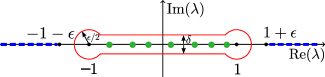
Figure 2: Contour $\gamma$ in the complex plane for $\lambda$ used to compute the von Neumann entropy of an interval [cf. Eq. (37)]. Dashed lines at $(-\infty,-1-\epsilon]\cup[1+\epsilon,\infty)$ denote a branch cut. Dots in the region $[-1,1]$ are the zeros of $D_{\ell}(\lambda)$ [cf. Eq. (36)], or, equivalently, the poles of $dD_{\ell}(\lambda)/d\lambda$. Here we are interested in the limits $\epsilon\to 0$ and $\delta\to 0$.

III Global Lindblad master equation

To make the paper self contained, we now recap the formalism used to treat self-consistently thermal baths in the Lindblad approximation, within quadratic models [18]. Let us consider the interaction between the fermionic chain $\mathcal{S}$ and the environment $\mathcal{E}$ (see Fig. 1). The global system $\mathcal{U}={\mathcal{S}}\cup\mathcal{E}$ is described by the Hamiltonian $H_{\mathcal{U}}=H_{\mathcal{S}}\otimes\mathds{1}_{\mathcal{E}}+\mathds{1}_{\mathcal{S}}\otimes H_{\mathcal{E}}+H_{I}$, where $H_{\mathcal{E}}$ is the Hamiltonian of the environment and $H_{I}$ models the interaction between system and environment. We can always write $H_{I}$ in the form

$$H_{I}=\sum_{\alpha}O_{\alpha}\otimes R_{\alpha},$$ (38)

where $O_{\alpha}$ and $R_{\alpha}$ are Hermitian operators acting on $\mathcal{S}$ and $\mathcal{E}$, respectively. In the following we restrict ourselves to the situation in which $O_{\alpha}$ act nontrivially only on a finite number of sites of the chain (see Fig. 1).

Given a state $\rho(t)$ of the entire system $\mathcal{S}\cup\mathcal{E}$, we are interested in the evolution of the reduced density matrix $\rho_{\mathcal{S}}(t)\coloneqq\Tr_{\mathcal{E}}[\rho(t)]$. In the Markovian regime, the dynamics is described by a Lindblad master equation of the form [15]

$$\frac{d\rho_{\mathcal{S}}(t)}{dt}=-i[H,\rho_{\mathcal{S}}(t)]+\mathcal{D}(\rho_{\mathcal{S}}(t)),$$ (39)

where both $H$ and $\mathcal{D}$ have to be determined. Let us assume that the environment consists of a finite number of uncorrelated fermionic infinite thermal baths, such that

$$H_{\mathcal{E}}=\sum_{\alpha}\int dp\,\varepsilon_{\alpha,p}\,d^{\dagger}_{\alpha,p}d_{\alpha,p},$$ (40)

where $\alpha$ is here an index that labels the bath, $d_{\alpha,p}$ the fermionic operators of the bath, and $\varepsilon_{\alpha,p}$ the bath dispersion. We also consider a generic linear coupling [cf. Eq. (38)] between the system and the baths:

$$O_{\alpha} =\sum_{j\in\mathcal{I}_{\alpha}}\left(a_{j}+a_{j}^{\dagger}\right),$$ (41)

$$R_{\alpha} =\int dp\,g_{\alpha,p}\left(d_{\alpha,p}+d^{\dagger}_{\alpha,p}\right),$$ (42)

where $g_{\alpha,p}$ is the strength of the coupling and $\mathcal{I}_{\alpha}$ are the sites of $\mathcal{S}$ that are coupled to the bath $\alpha$. Here we focus on the situation in which each bath is coupled to a single site of the system. For instance, for the case in Fig. 1(a), one has $\alpha=1,2$ with $\mathcal{I}_{1}=\{1\}$ and $\mathcal{I}_{2}=\{N\}$.

The dissipator $\mathcal{D}$ in Eq. (39) can be written as [18]

$$\mathcal{D}(\rho)=\sum_{\alpha,k}\Phi_{\alpha,k}\Big{[}\Gamma_{\alpha}(\omega_{k})\left(2b_{k}\rho b_{k}^{\dagger}-\{b_{k}^{\dagger}b_{k},\rho\}\right)\\ +\Gamma_{\alpha}(-\omega_{k})\left(2b_{k}^{\dagger}\rho b_{k}-\{b_{k}b_{k}^{\dagger},\rho\}\right)\Big{]}.$$ (43)

For simplicity we removed the subscript $\mathcal{S}$ in $\rho_{\mathcal{S}}$. The $b_{k}$’s denote the Bogoliubov operators that diagonalize the system [cf. Eq. (6)], whereas $\omega_{k}$ are the corresponding single-particle energies [cf. Eq. (5)]. Even though the interaction Hamiltonian $H_{I}$ is local in space, the dissipator $\mathcal{D}(\rho)$ is written in terms of nonlocal operators. In constrast, with common approaches, the Lindblad operators are chosen ad hoc and are typically local. Information about locality of the baths is encoded in the functions

$$\Phi_{\alpha,k}\coloneqq\bigg{|}\sum_{j\in\mathcal{I}_{\alpha}}\phi_{jk}\bigg{|}^{2}.$$ (44)

Moreover, we have defined [15]

$$\Gamma_{\alpha}(\omega)=\begin{cases}J_{\alpha}(\omega)(1-f_{\alpha}(\omega))&\omega>0,\\ J_{\alpha}(-\omega)f_{\alpha}(-\omega)&\omega<0,\end{cases}$$ (45)

which is written in terms of the Fermi-Dirac distribution $f_{\alpha}$ associated with the bath $\alpha$ at temperature $T_{\alpha}$ and chemical potential $\mu_{\alpha}$,

$$f_{\alpha}(\omega)=\frac{1}{1+e^{\beta_{\alpha}(\omega-\mu_{\alpha})}},\quad\beta_{\alpha}=\frac{1}{T_{\alpha}},$$ (46)

and the spectral density of the bath $\alpha$,

$$J_{\alpha}(\omega)=\pi\int dp\,|g_{\alpha,p}|^{2}\delta(\omega-\varepsilon_{\alpha,p}).$$ (47)

In the chosen diagonalization scheme we always have $\omega_{k}\geq 0$, hence we can also rewrite

$$\mathcal{D}(\rho)=\sum_{\alpha,k}\gamma_{\alpha,k}\Big{[}(1-f_{\alpha}(\omega_{k}))\left(2b_{k}\rho b_{k}^{\dagger}-\{b_{k}^{\dagger}b_{k},\rho\}\right)\\ +f_{\alpha}(\omega_{k})\left(2b_{k}^{\dagger}\rho b_{k}-\{b_{k}b_{k}^{\dagger},\rho\}\right)\Big{]},$$ (48)

where

$$\gamma_{\alpha,k}\coloneqq J_{\alpha}(\omega_{k})\Phi_{\alpha,k}.$$ (49)

Besides the dissipative effect encoded in $\mathcal{D}(\rho)$, the presence of the baths also renormalizes the unitary part of the Lindblad equation (39). Indeed, the effective Hamiltonian $H$ reads

$$H=\sum_{k}\widetilde{\omega}_{k}b_{k}^{\dagger}b_{k},$$ (50)

where the “dressed” single-particle dispersion $\widetilde{\omega}_{k}$ reads

$$\widetilde{\omega}_{k}=\omega_{k}\Bigg{(}1+\frac{2}{\pi}\sum_{\alpha}\Phi_{\alpha,k}\mathcal{P}\!\int_{0}^{\infty}\!\!\!d\epsilon\frac{J_{\alpha}(\epsilon)}{\omega_{k}^{2}-\epsilon^{2}}\Bigg{)},$$ (51)

with $\mathcal{P}$ denoting Cauchy’s principal value.

Crucially, the Lindblad equation (39) is derived by using a full secular approximation [15, 18, 19], which neglects rapidly oscillating terms $\propto\exp(i(\omega_{k}-\omega_{k^{\prime}})t)$. Moreover, we neglect degeneracy in the spectrum, assuming that $\omega_{k}\neq\omega_{k^{\prime}}$ if $k\neq k^{\prime}$. Both these approximations are in general uncontrolled, and checking their validity would require an ab initio treatment of the baths.

The master equation (39) is quadratic in the Bogoliubov operators $b_{k},b_{k}^{\dagger}$. This means that if the state of the system is Gaussian at a certain initial time, it will remain Gaussian at all subsequent times. Therefore, the state $\rho$ is completely determined by the two-point functions of the Majorana fermions (23). Equivalently, one can use the correlators $K_{kq}$ and $F_{kq}$ defined as

$$K_{kq} \coloneqq\mathrm{Tr}[\rho\,b^{\dagger}_{k}b_{q}],$$ (52a)

$$F_{kq} \coloneqq\mathrm{Tr}[\rho\,b_{k}b_{q}].$$ (52b)

A direct computation allows to obtain the evolution of $K_{kq}$ and $F_{kq}$ as [18]

$$\frac{dK_{kq}}{dt}=\Big{[}i(\widetilde{\omega}_{k}-\widetilde{\omega}_{q})-\sum_{\alpha}(\gamma_{\alpha,k}+\gamma_{\alpha,q})\Big{]}K_{kq}(t)\\ +2\delta_{kq}\sum_{\alpha}\gamma_{\alpha,k}f_{\alpha}(\omega_{k}),$$ (53a)

$$\frac{dF_{kq}}{dt}=\Big{[}-i(\widetilde{\omega}_{k}+\widetilde{\omega}_{q})-\sum_{\alpha}(\gamma_{\alpha,k}+\gamma_{\alpha,q})\Big{]}F_{kq}(t).$$ (53b)

Here $\widetilde{\omega}_{k}$ are the modified single-particle energies in Eq. (51), the rates $\gamma_{\alpha,k}$ are defined in Eq. (49), and $f_{\alpha}(\omega)$ is the Fermi-Dirac distribution of the bath [cf. Eq. (46)]. We anticipate that, for the setting in Fig. 1, due to the simple structure of Eqs. (12) and (20), the dependence on $\gamma_{\alpha,k}$ drops out. Assuming that $\gamma_{\alpha,k}$ are not all equal to zero (which is obviously true if the system is actually coupled to the environment), in the stationary limit $t\rightarrow\infty$ we obtain

$$K_{kq}=\delta_{kq}\frac{\sum_{\alpha}\gamma_{\alpha,k}f_{\alpha}(\omega_{k})}{\sum_{\alpha}\gamma_{\alpha,k}},\quad F_{kq}=0.$$ (54)

Thus the correlation function in momentum space becomes diagonal, and it is a convex combination of the Fermi-Dirac distributions of the baths. Equation (54) is the main ingredient to extract steady-state properties of the system (see Sec. IV and Sec. V). Note that, if the baths are identical ($f_{\alpha}$ does not depend on $\alpha$), we obtain $K_{kq}=\delta_{kq}f(\omega_{k})$. Interestingly, even in this situation, the statistical ensemble that describes the steady state is not the standard finite-temperature ensemble of the underlying free-fermion model, due to the nonzero chemical potential in Eq. (46). As we will show in the following, this implies that the steady-state von Neumann entropy exhibits logarithmic additive corrections to the expected volume-law scaling at finite temperature.

IV Scaling of entropy in the tight-binding chain

In this section we derive the scaling equation (3) of the steady-state von Neumann entropy for a subinterval of the tight-binding chain [cf. Eq. (9)]. A similar calculation was performed in Refs. [33, 34], but for a nonequilibrium setting which is different from ours.

First of all we recall that, from Eq. (30), $\Gamma$ has eigenvalues $\pm i\nu_{r}$ if and only if $G$ [cf. Eq. (29)] has eigenvalues $\nu_{r}$. We can exploit this fact by expressing the contour integral (37) in terms of

$$B_{\ell}(\lambda)\coloneqq\det(\lambda\mathds{1}-G_{A}),$$ (55)

finding

$$S_{A}=\lim_{\delta,\epsilon\to 0^{+}}\frac{1}{2\pi i}\oint_{\gamma}d\lambda\,e(1+\epsilon,\lambda)\frac{d\ln B_{\ell}(\lambda)}{d\lambda},$$ (56)

where $G_{A}$ is the matrix obtained from $G$ by restricting indices to $n,m\in A$, and $\ell=|A|$. Using the definitions of $\phi_{nk}$ and $\psi_{nk}$ reported in Eqs. (12), we find, in the limit $N\to\infty$,

$$G_{nm}=\int_{-\pi}^{\pi}\frac{dk}{2\pi}\,\widetilde{\theta}_{kk}\left[e^{ik(n-m)}-\zeta e^{ik(n+m)}\right],$$ (57)

where $\zeta=0$ and $\zeta=1$ corresponds to PBC and OBC, respectively. This equation defines a Toeplitz matrix for $\zeta=0$, whereas one has a Toeplitz-plus-Hankel matrix [42] for $\zeta=1$. The so-called symbol of $G_{nm}$ is

$$\widetilde{\theta}_{kk}\coloneqq\theta_{kk}\,\mathrm{sgn}(-h-2\cos k),$$ (58)

where $\theta_{kk}$ is given in Eq. (28) and the sign function is the same as in Eq. (12b). The function $\theta_{kk}$ encodes the information about the steady state and is obtained from (54). The function $\widetilde{\theta}_{kk}$ is smooth, except for the sign function which displays a singularity for $|h|<2$, thus giving rise to logarithmic corrections to the von Neumann entropy. Since the sign function comes from the Lieb-Schultz-Mattis matrices (12), the attentive reader could think that its appearance in the Majorana correlation matrix is an artifact originated from our choice of using the Bogoliubov modes to diagonalize the tight-binding Hamiltonian. However, in App. A we show that, if one constructs the master equation in terms of Fourier modes (which still diagonalize the Hamiltonian, but with continuous coefficients), then the discontinuity arises from their steady-state correlation function. As expected, physical quantities are not affected by this change and Eqs. (57) and (58) are unaltered.

To extract the scaling behavior of the mutual information (1) one has to determine the asymptotic scaling of the von Neumann entropy $S_{A}$ for a subsystem $A$ of length $\ell\to\infty$. To that purpose, we first study the asymptotic behavior of $B_{\ell}(\lambda)\equiv D_{\ell}[g_{\lambda}]$, being the determinant of the Toeplitz (or Toeplitz-plus-Hankel) matrix with symbol $g_{\lambda}(k)\coloneqq\lambda-\widetilde{\theta}_{kk}$ given by

$$g_{\lambda}(k)=\left\{\begin{array}[]{cl}\lambda-\theta_{kk}&\;\;k\in[-\pi,-k_{F}]\cup[k_{F},\pi),\\ \lambda+\theta_{kk}&\;\;k\in[-k_{F},k_{F}).\end{array}\right.$$ (59)

Since this symbol may have jump discontinuities at $\pm k_{F}$, we use the Fisher-Hartwig theorem to extract the scaling of $D_{\ell}[g_{\lambda}]$ for $\ell\to\infty$. The result is then substituted back in Eq. (56), from which the expression of the von Neumann entropy emerges. The details of the computation are reported in App. B, where we find

$$S_{A}=\alpha\ell+\frac{c(\Theta)}{3\nu}\ln(\ell)+\mathcal{O}(1),$$ (60)

where $\nu=1$ for PBC and $\nu=2$ for OBC. The prefactor of the linear term,

$$\alpha=-\int_{-\pi}^{\pi}\frac{dk}{2\pi}\Big{[}K_{kk}\ln(K_{kk})+(1-K_{kk})\ln(1-K_{kk})\Big{]},$$ (61)

is the von Neumann entropy per volume of the full system in the limit $N\to\infty$, i.e.,

$$\alpha=\lim_{\ell\to\infty}\frac{S_{A}}{\ell}=\lim_{N\to\infty}\frac{S_{N}}{N},$$ (62)

where we denoted with $S_{N}$ the entropy of the full system. For pure states one has either $K_{kk}=0$ or $K_{kk}=1$, which implies that $S_{N}=0$ and $\alpha=0$, as it should be. This is not the case in the presence of the environment, because the state is not pure. A similar behavior is typically observed in generic out-of-equilibrium quadratic fermionic and bosonic systems [24, 25, 26, 27].

The prefactor $c(\Theta)$ of the logarithm is nonvanishing only when the symbol (59) has the jump discontinuity (which happens precisely when the model is critical), and it is given by

$$c(\Theta)=\frac{3}{\pi^{2}}\!\left[(1+\Theta)\mathrm{Li}_{2}\!\left(\frac{2\Theta}{\Theta+1}\right)\!+\!(1-\Theta)\mathrm{Li}_{2}\!\left(\frac{2\Theta}{\Theta-1}\right)\right]\!,$$ (63)

where $\Theta\coloneqq\theta_{kk}\evaluated{}_{k=k_{F}}$ is the steady-state density of Bogoliubov excitations at the Fermi level, which contains information about the environment, and

$$\mathrm{Li}_{2}(x)=-\int_{0}^{x}dz\,\frac{\ln(1-z)}{z}$$ (64)

is the dilogarithm function [51]. This result is somewhat reminiscent of the effective central charge obtained in free-fermion chains in the presence of defects [52, 53, 54, 55, 56]. Formally, this expression is a special symmetric case of the result obtained in Ref. [33], which is valid for two arbitrary asymmetric jumps in the symbol. For $\Theta\to 1$, which corresponds to the ground state of the closed chain, one recovers the standard central charge $c=1$, since $\mathrm{Li}_{2}(1)=\pi^{2}/6$. Instead, in the opposite limit $\Theta\to 0$ one obtains that $c(\Theta)$ vanishes, since $\mathrm{Li}_{2}(0)=0$. The behavior of $c(\Theta)$ as a function of $\Theta$ is illustrated in Fig. 3.

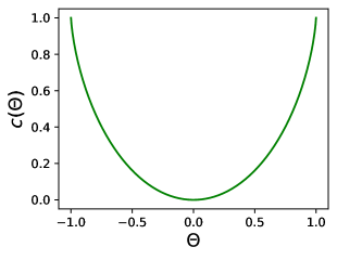
Figure 3: Effective central charge $c(\Theta)$ in Eq. (63) for the tight-binding chain coupled to localized thermal baths. Here $\Theta\in[-1,1]$ encodes the information about the baths. For a single bath at the left edge of the chain, $\Theta$ is given by Eq. (67). For two baths at the edges of the chain, $\Theta$ is given by Eq. (71). In the limit $|\Theta|\to 1$, one recovers the CFT result $c=1$. For $\Theta\to 0$ one has $c\to 0$, which corresponds to a high-temperature limit.

IV.1 Single bath

To illustrate our results, we first focus on the tight-binding chain with OBC and with only one edge coupled to a bath with temperature $T_{L}$ and chemical potential $\mu_{L}$ (see Fig. 1). In the steady state, from Eq. (54) we have

$$K_{kq}=\langle b^{\dagger}_{k}b_{q}\rangle=\delta_{kq}f(\omega_{k}),$$ (65)

where $\omega_{k}$ are the single-particle energies [cf. Eq. (10)], and $f(\omega_{k})$ is the Fermi-Dirac distribution describing the bath [cf. Eq. (46)]. Eq. (65) implies that the function $\theta_{kk}$ [cf. (28)] is given by

$$\theta_{kk}=1-2f(\omega_{k}).$$ (66)

Thus, we have

$$\Theta=\theta_{kk}\evaluated{}_{k=k_{F}}=1-2f(0)=\tanh(-\frac{\mu_{L}}{2T_{L}}).$$ (67)

Notice that $\Theta$ depends only on the ratio $\mu_{L}/T_{L}$. The limit $\mu_{L}/T_{L}\to 0$ gives $\Theta\to 0$ and a vanishing $c(\Theta)$ (see Fig. 3), so that the logarithmic correction to the entropy disappears. This regime corresponds to either infinite temperature $T_{L}\to\infty$ or vanishing chemical potential $\mu_{L}\to 0$. On the other hand, for $|\mu_{L}/T_{L}|\to\infty$ we have $|\Theta|\to 1$, so that $c\to 1$. Moreover, in this limit $K_{kk}\to 0$ or $K_{kk}\to 1$, which implies that $\alpha\to 0$ [cf. (61)]. Thus, we recover the ground-state scaling of the von Neumann entropy.

IV.2 Two baths

Let us now discuss the case with two different thermal baths, first considering the simpler case of PBC. Under the assumption that the spectral density $J(\omega)$ [cf. (47)] is the same for the two baths, we have for the couplings

$$\gamma_{L,k}=\gamma_{R,k}=\frac{J(\omega_{k})}{N},$$ (68)

since, from Eq. (12a), we have $|\phi_{1k}|^{2}=|\phi_{Nk}|^{2}=1/N$. Using Eq. (54), we therefore obtain

$$K_{kq} =\delta_{kq}\frac{f_{L}(\omega_{k})+f_{R}(\omega_{k})}{2},$$ (69)

$$\theta_{kk} =\frac{1}{2}\left[\tanh\left(\frac{\omega_{k}-\mu_{L}}{2T_{L}}\right)+\tanh\left(\frac{\omega_{k}-\mu_{R}}{2T_{R}}\right)\right].$$ (70)

Notice that the correlator $K_{kq}$ does not depend on the couplings $\gamma_{L/R,k}$. Moreover, as is clear from (69), the steady-state correlator is written in terms of the average between the Fermi-Dirac distributions describing the baths. From Eq. (70) we obtain

$$\Theta=\frac{1}{2}\left[\tanh\left(-\frac{\mu_{L}}{2T_{L}}\right)+\tanh\left(-\frac{\mu_{R}}{2T_{R}}\right)\right].$$ (71)

Notice that $\Theta$ depends only the ratios $\mu_{L}/T_{L}$ and $\mu_{R}/T_{R}$, which is structurally similar to what we obtained in the single-bath scenario.

In the case of OBC and baths placed at the edges of the chain [see Fig. 1(a)], one has for the couplings

$$\gamma_{L,k} =J(\omega_{k})\frac{2\sin^{2}(k)}{N+1},$$ (72a)

$$\gamma_{R,k} =J(\omega_{k})\frac{2\sin^{2}(kN)}{N+1}.$$ (72b)

Making use of the quantization condition on $k$, one can show with a straightforward calculation that Eqs. (69), (70), and (71) continue to remain valid.

V Scaling of entropy in the Kitaev chain

We now turn to the steady-state von Neumann entropy in the Kitaev chain with PBC. The blocks of the Majorana correlation matrix $\Gamma$ are reported in Eq. (32), where we recognize a Toeplitz structure. Given a subsystem $A$, we are interested in the matrix $\lambda\mathds{1}-i\Gamma_{A}$ [cf. Eq. (36)], which is then also of the Toeplitz type. Let us define its symbol $g_{\lambda}(k)$ [cf. (32)] as

$$g_{\lambda}(k)=\begin{bmatrix}\lambda&-i\theta_{kk}e^{-i\xi(k)}\\ i\theta_{kk}e^{i\xi(k)}&\lambda\end{bmatrix}.$$ (73)

In contrast with the tight-binding chain, for which it was a scalar, now the symbol is a two-by-two matrix. At zero temperature, the asymptotic behavior in the large-$\ell$ limit of the determinant of the Toeplitz matrix (32) has been obtained in Ref. [57]. Here we are only interested in the logarithmic correction to the volume-law scaling of the von Neumann entropy. Thus, we can use the techniques of Refs. [58, 59]. The idea is that since the logarithmic correction depends only on the singularities of the symbol, we are allowed to modify the latter, provided that we do not change its singularity structure. This eventually allows one to work with a scalar symbol. The computation is rather technical and we leave the details to App. C. The result is analogous to the tight-binding case:

$$S_{A}=\alpha\ell+\frac{c^{\prime}(\Theta)}{3}\ln(\ell)+\mathcal{O}(1),$$ (74)

where $\alpha$ is the same constant reported in (61) and $c^{\prime}(\Theta)$ is half of the effective central charge of the tight-binding model, provided $|h|=2$:

$$c^{\prime}(\Theta)=\frac{c(\Theta)}{2}.$$ (75)

This time we have

$$\Theta=\begin{cases}\theta_{kk}\evaluated{}_{k=\pi}&h=2,\\ \theta_{kk}\evaluated{}_{k=0}&h=-2,\end{cases}$$ (76)

in accordance with the discussion at the end of Sec. II.1.2. Clearly, in the zero-temperature limit $\Theta\to 1$ we recover the well-known central charge $c=1/2$ of the critical Kitaev chain.

This result is valid for a general value of $\theta_{kk}$, and we can easily specialize the expression of $\Theta$ to the steady state (54) of our master equation. Since with PBC the matrix $\phi_{nk}$ is equal to the corresponding matrix for the tight-binding chain [compare Eq. (12a) with Eq. (20a)], one finds for $K_{kq}$, $\theta_{kk}$, and $\Theta$ the same quantities reported in Eqs. (65)-(67) and Eqs. (69)-(71) for the single-bath and two-bath geometries, respectively. In the case $\mu_{L}=\mu_{R}=0$ and $T_{L}=T_{R}=T$ one recovers the correlator for the finite-temperature Kitaev (and Ising) chain [60, 61, 62] at temperature $T$. For $T\to 0$ one finds $\theta_{kk}\to 1$, thus recovering the zero-temperature correlator of the Kitaev chain. Importantly, the presence of $\mu_{L}$ and $\mu_{R}$ in (70) implies that the statistical ensemble describing the steady state is not the usual finite-temperature ensemble of the Kitaev chain.

VI Numerical results

We now provide numerical benchmarks for the results of Sec. IV and Sec. V. In particular, we numerically diagonalize the Majorana correlation matrix (26) for our models and then we use its eigenvalues to directly evaluate entropic quantities using Eq. (34). The results are then compared to what we derived in an analytical way. In Sec. VI.1 we overview the behavior of the subsystem von Neumann entropy. Our main results are contained in Sec. VI.2, where we discuss the scaling behavior of the steady-state mutual information both for the tight-binding chain (Sec. VI.2.1) and for the Kitaev chain (Sec. VI.2.2). Our numerical results confirm a logarithmic scaling for the mutual information, being in perfect agreement with the predictions of the previous sections. Finally, in Sec. VI.3 we briefly argue that logarithmic scaling also occurs for the fermionic logarithmic negativity, thus suggesting that the growth of the mutual information reflects a logarithmic entanglement growth.

VI.1 Volume-law scaling of von Neumann entropy

In the presence of the external baths, the steady-state von Neumann entropy exhibits a volume-law scaling as $\alpha\ell$, with $\ell$ being the size of the subsystem and $\alpha$ being the constant reported in Eq. (61), which equals the density of the von Neumann entropy of the full system. In the absence of baths, the full system is in a pure state, and its von Neumann entropy is zero ($\alpha=0$). The volume-law scaling in the open setting is due to the fact that the steady state is described by a finite-temperature-like statistical ensemble [63, 64].

Here we focus on the tight-binding chain with OBC and one thermal bath [see Fig. 1(a)]. Results for different boundary conditions and for the Kitaev chain are qualitatively similar and will not be discussed.

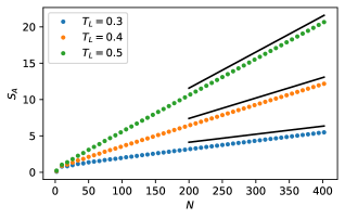
Figure 4: Volume-law scaling of the von Neumann entropy in the open tight-binding chain with a single bath on the left edge of the system (see Fig. 1). Subsystem $A$ is the half chain ($\ell=N/2$). Here we choose $h=1$, $\mu_{L}=-1$, and ${T_{L}=0.3,0.4,0.5}$. Straight lines denote the analytic predictions for the volume-law scaling, in the limit $\ell\to\infty$ [cf. Eq. (60)]. The logarithmic correction is not clearly visible at this scale.

Figure 4 reports the von Neumann entropy $S_{A}$ as a function of the chain length $N$, where the subsystem $A$ is the half-chain with $\ell=N/2$ [cf. Fig. 1(a)]. Only the left edge is in contact with a thermal bath at chemical potential $\mu_{L}=-1$ and temperature $T_{L}$. Data in the figure correspond to different temperatures $T_{L}$. A robust growth is visible at all temperatures, with a slope that decreases as the temperature is lowered. This is expected, since at $T=0$ the scaling of the von Neumann entropy is logarithmic with the interval size. Continuous lines show the expected linear behavior as $\alpha\ell$ in the limit $\ell\to\infty$, with a prefactor $\alpha$ given by Eq. (61). We observe a qualitative agreement with the theoretical predictions, at least to the leading order in $\ell$. However, as also expected from Eq. (60), subleading logarithmic corrections are present. To reveal them it is convenient to use the mutual information.

VI.2 Logarithmic scaling of mutual information

We now discuss the scaling of the steady-state mutual information in the presence of external baths. The logarithmic prefactor is determined by the singular structure of the single-particle energy dispersion, as discussed in Sec. IV and Sec. V.

VI.2.1 Tight-binding chain

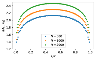
Figure 5: Mutual information $I(A_{1}:A_{2})$ between two intervals in the open tight-binding chain with a thermal bath on the left edge. Here we choose $\mu_{L}=-1$, $T_{L}=0.3$, and $h=1$. Different colors correspond to different chain length $N$. The data are plotted versus $\ell/N$, with $\ell$ being the size of $A_{1}$ (see Fig. 1(a)). Notice the symmetry under exchange of the two subsystems $\ell\leftrightarrow N-\ell$.

For the tight-binding model of Eq. (9), we consider the same setup as in Sec. IV.1, i.e, the open chain with a thermal bath on the left edge. We fix $h=1$, $\mu_{L}=-1$, and $T_{L}=0.3$. Our numerical data for the mutual information $I(A_{1}:A_{2})$ between two complementary intervals $A_{1}$ and $A_{2}=\overline{A}_{1}$ are plotted in Fig. 5 versus $\ell/N$, with $\ell$ being the size of $A_{1}$. The three different data sets correspond to different values of $N$. At each fixed $N$, $I(A_{1}:A_{2})$ increases upon increasing $\ell$ up to $\ell\sim N/2$, after which it starts decreasing. The behavior at intermediate $1\ll\ell\ll N$ is consistent with a logarithmic increase, as predicted in Eq. (60), which should hold in the limit $N\to\infty$ and then $\ell\to\infty$ (with this order of limits).

Looking now at the definition of the mutual information [cf. Eq. (1)], it is clear that, when constructing $I(A_{1}:A_{2})$, the volume-law terms in the entropies cancel out. To derive the prefactor of the logarithmic scaling, we can use Eq. (60) for each term appearing in (1). Notice that no logarithmic contribution is expected from $S_{A_{1}\cup A_{2}}$, since the entropy of the full system for large $N$ is exactly $\alpha N$, with $\alpha$ given by (61). Let us also stress that, in principle, we are not allowed to use Eq. (60) for $S_{A_{2}}$ because the size $N-\ell$ of $A_{2}$ is comparable with $N$. To proceed, we should then conjecture a generalization for an interval $A$ of generic size, embedded in a finite-size chain. Following the standard strategy for critical systems described by CFTs, we write [65]

$$S_{A}=\alpha\ell+\frac{c(\Theta)}{6}\ln\left[\frac{N}{\pi}\sin\left(\frac{\pi\ell}{N}\right)\right]+{\mathcal{O}}(1).$$ (77)

Notice that the prefactor of the volume-law term is the same as before, while in the logarithmic term of Eq. (60) we replaced

$$\ell\to X_{\ell},\quad\mathrm{with}\,\,X_{\ell}\coloneqq\frac{N}{\pi}\sin\left(\frac{\pi\ell}{N}\right),$$ (78)

where $X_{\ell}$ is the so-called chord length. Eq. (77) holds in the thermodynamic limit $\ell,N\to\infty$. For systems with boundaries, as is the case here, the actual chord length differs from (78) by an overall factor $2$, which only affects the ${\mathcal{O}}(1)$ term, and can therefore be neglected. We conclude that

$$I(A_{1}:A_{2})=\frac{c(\Theta)}{3}\ln\left[\frac{N}{\pi}\sin\left(\frac{\pi\ell}{N}\right)\right]+{\mathcal{O}}(1).$$ (79)

The factor $1/3$ rather than $1/6$ is due to the fact that both subsystems $A_{1}$ and $A_{2}$ contribute with a logarithmic term. Importantly, Eq. (79) implies that for large $\ell,N$ the data for the mutual information should collapse on the same curve, when plotted as a function of $X_{\ell}$.

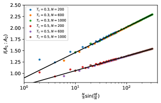
Figure 6: Mutual information $I(A_{1}:A_{2})$ between two complementary intervals [see Fig. 1(a)] in the open tight-binding chain with a thermal bath on the left edge. On the $x$-axis $N\sin(\pi\ell/N)/\pi\equiv X_{\ell}$ is the chord length. Data are for fixed $\mu_{L}=-1$, $h=1$, and for $T_{L}=0.3,0.5$, while the various colors denote different $N$. The lines are fits to $c(\Theta)\ln(X_{\ell})/3+b$, $c(\Theta)$ being the effective central charge [cf. Eq. (63)] and $b$ a fitting constant parameter.

The validity of Eq. (79) is investigated in Fig. 6 for the tight-binding chain with one thermal bath on the left edge. We consider two different temperatures ${T_{L}=0.3,0.5}$ at fixed $\mu_{L}=-1$. The mutual information $I(A_{1}:A_{2})$ is plotted versus $X_{\ell}$ (notice the logarithmic scale on the $x$-axis) for several values of ${N=200,600,1000}$. For both temperatures, the data exhibit collapse. The quality of the collapse improves upon increasing $N$, as expected. Continuous lines are fits to Eq. (79), where $c(\Theta)$ is kept fixed and given by Eq. (63), while the additive ${\mathcal{O}}(1)$ term being the only fitting parameter. For both temperatures, the agreement between the data and the fits is very satisfactory.

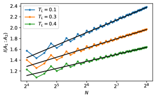
Figure 7: Scaling of the half-chain mutual information in the open tight-binding chain with a thermal bath of the left edge of the chain. Here we fix $\mu_{L}=-1$, $h=1$. Different colors are for different values of $T_{L}$. Continuous lines are fits to $a\ln(N)+b$, with $a,b$ fitting parameters.

Eq. (79) also implies that, for large $N$, the mutual information between the two halves of the chain scales logarithmically as $c(\Theta)\ln(N)/3$. This is shown in Fig. 7, for the same setup as in Fig. 6. The various data sets correspond to different temperatures of the external bath. The logarithmic increase is clearly visible (notice the semilog scale), although oscillating corrections are present. The continuous lines are fits to

$$I(A_{1}:A_{2})=a\ln(N)+b,$$ (80)

with $a,b$ fitting parameters. Further checks of our results are provided in Fig. 8 where, for each temperature, we numerically extract $c(\Theta)$ by fitting the mutual information to Eq. (80). Symbols are the results of the fits, which are obtained as in Fig. 7 fitting the data with $N>2^{6}$. At low temperature, one finds $c(\Theta)\to 1$, whereas $c(\Theta)$ vanishes in the high-temperature limit. The continuous line is the analytic prediction in the limit $N\to\infty$, given by Eq. (63). The agreement with the numerics is excellent.

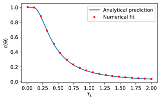
Figure 8: The effective central charge $c(\Theta)$ versus the temperature $T_{L}$, as obtained from fits of numerical data as those in Fig. 7. Parameters are the same as in Fig. 7.

Finally we discuss a two-bath geometry, where the edges of the chain are connected to two different thermal baths. We fix $h=1$ and we consider two situations: constant temperature $T_{L}=T_{R}=1$ with $\mu_{L}=0$ fixed, and constant chemical potential $\mu_{L}=\mu_{R}=-1$ with $T_{L}=1$ fixed. In Fig. 9 we plot the numerically extracted $c(\Theta)$ versus $\mu_{R}$ and $T_{R}$, respectively, for the two scenarios. As for Fig. 8, the continuous line denotes the theoretical result in the limit $N\to\infty$, which is in perfect agreement with the numerics.

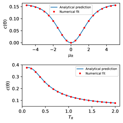
Figure 9: Logarithmic scaling of the mutual information $I(A_{1}:A_{2})$ in the tight-binding chain with OBC coupled to two thermal baths at the edges. In the upper panel, we plot $c(\Theta)$ versus $\mu_{R}$, for fixed $T_{L}=T_{R}=1$ and $\mu_{L}=0$. In the lower panel, we plot $c(\Theta)$ versus $T_{R}$, for fixed ${\mu_{L}=\mu_{R}=-1}$ and $T_{L}=1$. In both cases, $h=1$. Numerical results for $c(\Theta)$ are obtained by performing a finite-size scaling analysis for the half-chain mutual information.

VI.2.2 Kitaev chain

Let us now discuss the steady-state mutual information in the Kitaev chain. Here we consider a PBC geometry, as depicted in Fig. 1(b). Two sites at mutual distance $N/2$ are put in contact with two external baths at temperatures $T_{R/L}$ and with chemical potentials $\mu_{R/L}$. We choose $T_{L}=T_{R}=1$, $\mu_{L}=0$, $\mu_{R}=2,4$, and fix $h=2$. We consider the mutual information $I(A_{1}:A_{2})$ between two intervals of size $\ell$ and $N/2-\ell$ placed between the baths (see Fig. 1). First, we should observe that in constructing the mutual information (1) all the entropies (i.e., $S_{A_{1}}$, $S_{A_{2}}$, and $S_{A_{1}\cup A_{2}}$) contain a subleading logarithmic term. This happens because $S_{A_{1}\cup A_{2}}$ is not the full system. As for the tight-binding chain the volume-law terms, instead, cancel out. The final result is

$$I(A_{1}:A_{2})=\frac{c^{\prime}(\Theta)}{3}\ln(X_{2\ell})+{\mathcal{O}}(1),$$ (81)

where $X_{2\ell}$ is the chord length in Eq. (78) (notice the factor $2$), and $c^{\prime}(\Theta)=c(\Theta)/2$ is the effective central charge calculated for the Kitaev chain [cf. Eq. (74)]. To derive Eq. (81) we used the fact that, for all the intervals $A_{1}$, $A_{2}$, and $A_{1}\cup A_{2}$,

$$S_{W}\xrightarrow[]{\ell,N\to\infty}\frac{c^{\prime}(\Theta)}{3}\ln(X_{\ell}),\quad W=A_{1(2)},A_{1}\cup A_{2},$$ (82)

After substituting (82) in the definition of the mutual information (1), we obtain (81). We point out that Eq. (81) holds only for the geometry in Fig. 1(b), although it could be easily generalized to more general settings.

The validity of Eq. (81) is numerically verified in Fig. 10, where we plot $I(A_{1}:A_{2})$ versus $X_{2\ell}$. For both values of $\mu_{R}$, the data exhibit collapse at large $\ell,N$. Continuous lines are fits to Eq. (81), the only fitting parameter being the ${\mathcal{O}}(1)$ constant. The agreement between the analytic prediction in the scaling limit $\ell,N\to\infty$ and the numerics is nearly perfect already for relatively small chains with $X_{2\ell}\sim 10$.

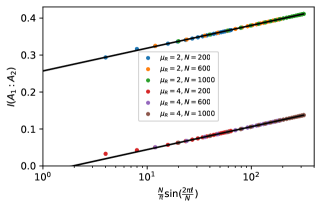
Figure 10: Mutual information $I(A_{1}:A_{2})$ between two intervals in the Kitaev chain with PBC and two external baths [see Fig. 1(b)] versus the chord length $X_{2\ell}=N\sin(2\pi\ell/N)/\pi$. Here we choose $T_{L}=T_{R}=1$, $\mu_{L}=0$ and $\mu_{R}=2,4$. The various symbols correspond to different chain sizes $N$. Continuous lines are fits to $I(A_{1}:A_{2})=c(\Theta)\ln(X_{2\ell})/6+b$, with $c(\Theta)$ the effective central charge, and $b$ a fitting constant.

VI.3 Fermionic logarithmic negativity

In general, the mutual information between two subsystems does not provide a measure of quantum entanglement between them, since it contains information also about classical correlations. Given $A=A_{1}\cup A_{2}$ in a mixed state $\rho_{A}$, a proper measure of entanglement between $A_{1}$ and $A_{2}$ is given by the fermionic logarithmic negativity [28, 29], defined as

$$\mathcal{E}(A_{1}:A_{2})=\ln\norm{\rho_{A}^{R_{1}}},$$ (83)

where $\norm{X}=\Tr\sqrt{XX^{\dagger}}$ is the trace norm and $\rho_{A}^{R_{1}}$ stands for the operator obtained after performing a partial time-reversal transformation on $\rho_{A}$ with respect to $A_{1}$ (notice that this is different from the standard logarithmic negativity defined for bosonic systems [66]). The fermionic logarithmic negativity can be efficiently calculated numerically for fermionic Gaussian states [28], and this applies in particular to our steady state.

Let us consider, as an example, the fermionic logarithmic negativity between two halves of a tight-binding chain with OBC. In the ground state of the isolated chain it is known that the fermionic logarithmic negativity exhibits logarithmic scaling with a prefactor of $c/4$ [28]. In Fig. 11 we report an example of calculation with our steady state in the two-bath geometry. We clearly observe logarithmic scaling, suggesting that such a feature is of quantum nature. However, the prefactor is not consistent with a straightforward generalization $c/4\to c(\Theta)/4$, hence further studies are necessary in order to establish its exact value in the nonequilibrium scenario. Similar conclusions apply for the Kitaev chain.

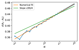
Figure 11: Scaling of the half-chain fermionic logarithmic negativity (83) in the tight-binding chain with OBC and two thermal baths at the edges. Here the parameters are ${h=1}$, ${\mu_{L}=-1}$, ${\mu_{R}=-1.5}$, ${T_{L}=1}$, ${T_{R}=1.5}$. The orange line is a linear fit in logarithmic scale, while the green line is $(c(\Theta)/4)\ln N+b$ with $b$ a fitting constant.

VII Conclusions

We investigated the quantum-information spreading in the tight-binding chain and the Kitaev chain in the presence of external thermal baths coupled to individual sites of the chains. To this purpose, we employed a self-consistent nonlocal Lindblad master equation approach, where the Lindblad operators modeling the baths are written in terms of the Bogoliubov modes that diagonalize the isolated system, implying that they are, in principle, nonlocal in real space [18]. The statistical ensemble describing the steady state is written in terms of a convex combination of the Fermi-Dirac distributions of the baths. We showed that the steady-state von Neumann entropy of a subsystem exhibits a volume-law scaling with the subsystem size, reflecting that the system is not in a pure state. The mutual information exhibits an area-law scaling for generic values of the system parameters. Interestingly, we observe logarithmic violations of the area law in the presence of ground-state criticality. This behavior reflects the singularity of the single-particle energy dispersion of the models, which is present at all energies. We analytically derived the prefactor of the logarithmic growth of the mutual information, which depends on the system and bath parameters, such as the temperature and the chemical potential.

Let us now mention some promising directions for future work. First of all, here we only analyzed the steady-state value of the mutual information: it would be tempting to study the full-time dynamics, in order to establish how the logarithmic scaling builds up during the evolution of the system. A natural conjecture is that the same effective central charge governs a logarithmic increase in time, as in Ref. [34]. Our analysis may be also extended to genuine quantum entanglement measures for mixed states, such as the fermionic logarithmic negativity. Finally, it would be important to check the validity of our results by comparing them with ab initio numerical simulations, or with results obtained using different master equations. A crucial question to address is whether the logarithmic scaling of the mutual information would survive in interacting integrable systems (or even in nonintegrable ones), or in the presence of non-Markovian interactions with the environment.

Appendix A Tight-binding model in terms of Fourier modes

In this appendix we argue that the presence of the discontinuity in the symbol (57) is not artificially introduced by our choice of the basis with which we diagonalized the tight-binding Hamiltonian (9), that is performed with discontinuous coefficients (12). Specifically, let us consider a tight-binding chain with PBC and define Fourier modes $c_{k}$ through

$$a_{n}=\frac{1}{\sqrt{N}}\sum_{k}e^{-ikn}c_{k}.$$ (84)

In the basis $\{c_{k}\}$ the Hamiltonian is diagonalized, as in (5), but with single-particle energies

$$\omega_{k}=-h-2\cos(k).$$ (85)

The master equation of Ref. [18] can be derived in a straightforward way to obtain Eq. (43), but with the substitution $b_{k}\to c_{k}$. However, Eq. (48) is no longer valid because $\omega_{k}$ may be negative. The calculation of the steady-state correlation functions can still be performed starting directly from Eq. (43). Using the relation $\Gamma_{\alpha}(\omega)+\Gamma_{\alpha}(-\omega)=J_{\alpha}(|\omega|)$ we find

$$\langle c_{k}^{\dagger}c_{k}\rangle=\frac{\sum_{\alpha}\Phi_{\alpha,k}\Gamma_{\alpha}(-\omega_{k})}{\sum_{\alpha}\Phi_{\alpha,k}J_{\alpha}(|\omega_{k}|)}=\begin{cases}\langle b_{k}^{\dagger}b_{k}\rangle&\omega_{k}>0,\\ 1-\langle b_{k}^{\dagger}b_{k}\rangle&\omega_{k}<0,\end{cases}$$ (86)

where $\langle b_{k}^{\dagger}b_{k}\rangle$ is the standard Bogoliubov correlator reported in (54) with $\omega_{k}\to|\omega_{k}|$. If the model is critical, then $\langle c_{k}^{\dagger}c_{k}\rangle$ is discontinuous as a function of $k$.

If we now define the Majorana operators in terms of $c_{k}$, we obtain [cf. Eq. (57)]

$$G_{nm}=\int_{-\pi}^{\pi}\frac{dk}{2\pi}(1-2\langle c_{k}^{\dagger}c_{k}\rangle)e^{ik(n-m)},$$ (87)

which, in terms of $\langle b_{k}^{\dagger}b_{k}\rangle$, becomes

$$G_{nm}=\int_{-\pi}^{\pi}\frac{dk}{2\pi}\mathrm{sgn}(\omega_{k})(1-2\langle b_{k}^{\dagger}b_{k}\rangle)e^{ik(n-m)},$$ (88)

which is identical to Eq. (57). Therefore, the von Neumann entropy is unaltered by this change of basis, as expected.

Appendix B Calculation for the tight-binding chain

In this appendix we show how to perform the calculation of the steady-state von Neumann entropy for the tight-binding chain (cf. Sec. IV).

Let us first consider the case of PBC, i.e., $\zeta=0$ in Eq. (57). From that equation we obtain

$$\lambda\delta_{nm}-G_{nm}=\int_{-\pi}^{\pi}\frac{dk}{2\pi}e^{ik(n-m)}g_{\lambda}(k).$$ (89)

This defines a Toeplitz matrix, hence we can apply the Fisher-Hartwig theorem [38, 39, 40] to evaluate its determinant for large $\ell$. Such theorem has been already employed in the literature to determine the scaling behavior of the von Neumann and Rényi entropies in the ground state of critical fermionic chains [44, 67, 43]. Here we apply a specialized version in which the symbol $g_{\lambda}(k)$ is allowed to have only jump discontinuities at a finite number of points $k_{r}$. In order to apply the theorem one has to rewrite $g_{\lambda}(k)$ in the form

$$g_{\lambda}(k)=g_{s}(k)\prod_{r=1}^{R}e^{ib_{r}(k-k_{r}-\pi\,\mathrm{sgn}(k-k_{r}))}.$$ (90)

Here $g_{s}(k)$ is a smooth function of $k$, $R$ is the number of discontinuities of the symbol, and $b_{r},k_{r}$ are real constants. The Fisher-Hartwig theorem states that, in the limit $\ell\to\infty$, one has

$$D_{\ell}[g_{\lambda}]\sim F[g_{s}]^{\ell}\Bigg{(}\prod_{j=1}^{R}\ell^{-b_{j}^{2}}\Bigg{)}E[g_{\lambda}],$$ (91)

where we defined

$$F[g_{s}]\coloneqq\exp\left(\int_{-\pi}^{\pi}\frac{dk}{2\pi}\ln g_{s}(k)\right).$$ (92)

From Eq. (37) it is clear that the first factor in (91) gives a volume-law von Neumann entropy, and it is not sensitive to the singularities in the symbol $g_{\lambda}(k)$. The second factor is responsible for the logarithmic scaling of the von Neumann entropy and contains information about the singularities of $g_{\lambda}(k)$. The constant $E$ is a known function of $g_{\lambda}(k)$. In the following, we are not considering $E$ because we are interested only in the linear growth of the von Neumann entropy and in the logarithmic correction.

It is straightforward to check that in our case the symbol $g_{\lambda}(k)$ in (59) can be written in the form (90) with two discontinuities at $k_{1}=-k_{F}$ and $k_{2}=k_{F}$, i.e., with $R=2$, and

$$b_{1}=-b_{2}=\beta_{\lambda}+m,$$ (93)

where $m$ is an integer and

$$\beta_{\lambda}=\frac{1}{2\pi i}\ln\left(\frac{\lambda-\Theta}{\lambda+\Theta}\right),\quad\Theta\coloneqq\theta_{kk}\evaluated{}_{k=k_{F}}.$$ (94)

The function $g_{s}(k)$ is given by

$$g_{s}(k)=\left(\frac{\lambda+\Theta}{\lambda-\Theta}\right)^{\frac{k_{F}}{\pi}-1}(\lambda+\theta_{kk})\Theta_{\mathrm{H}}(k_{F}-|k|)\\ +\left(\frac{\lambda+\Theta}{\lambda-\Theta}\right)^{\frac{k_{F}}{\pi}}(\lambda-\theta_{kk})\Theta_{\mathrm{H}}(|k|-k_{F}).$$ (95)

Now, we have to substitute Eqs. (93), (94), and (95) in Eq. (91). The first factor in Eq. (91) determines the constant $\alpha$ in Eq. (60). By using (56) one obtains

$$\alpha\!=\!\lim_{\delta,\epsilon\to 0^{+}}\frac{1}{4\pi^{2}i}\oint_{\gamma}d\lambda\int_{-\pi}^{\pi}dk\frac{e(1+\epsilon,\lambda)}{\lambda+\mathrm{sgn}(k_{F}-|k|)\theta_{kk}},$$ (96)

where $e(x,\nu)$ is defined in (35), $\theta_{kk}$ in (28), and $\gamma$ denotes the contour shown in Fig. 2. This integral can be performed with the residue theorem, leading to

$$\alpha=\int_{-\pi}^{\pi}\frac{dk}{2\pi}e(1,\theta_{kk}),$$ (97)

which is precisely the expression reported in Eq. (61).

The second factor in Eq. (91) yields for the prefactor of the logarithmic term (cf. Eq. (60) with $\nu=1$)

$$\frac{c(\Theta)}{3}=\lim_{\delta,\epsilon\rightarrow 0^{+}}\frac{1}{\pi i}\oint_{\gamma}d\lambda\,e(1+\epsilon,\lambda)\frac{d(-\beta_{\lambda}^{2})}{d\lambda},$$ (98)

where $\beta_{\lambda}$ is defined in Eq. (94) and, again, $\gamma$ denotes the “dogbone” contour in Fig. 2. We can perform an integration by parts to obtain

$$\frac{c(\Theta)}{3}=\lim_{\delta,\epsilon\rightarrow 0^{+}}\frac{1}{8\pi^{3}i}\oint_{\gamma}d\lambda\,\ln^{2}\left(\frac{\lambda+\Theta}{\lambda-\Theta}\right)\ln(\frac{1+\epsilon+\lambda}{1+\epsilon-\lambda}).$$ (99)

The contribution of the circles around $\pm 1$ in $\gamma$ (see Fig. 2) vanishes in the limit $\epsilon\to 0^{+}$. The integration along the horizontal paths can be performed using the fact that, for $\delta\to 0^{+}$, one has

$$\ln(\frac{x\pm i\delta+t}{x\pm i\delta-t})\to\ln\left|\frac{t+x}{t-x}\right|\mp i\pi\,\text{sgn}(t)\Theta_{\mathrm{H}}(|t|-|x|).$$ (100)

Inserting in (99), this gives

$$\frac{c(\Theta)}{3}=\frac{1}{2\pi^{2}}\int_{-\Theta}^{\Theta}dx\ln(\frac{\Theta+x}{\Theta-x})\ln(\frac{1+x}{1-x}).$$ (101)

This integral can be expressed in terms of dilogarithm functions (64): the result is reported in Eq. (63).

Let us now discuss the case with OBC and consider a block of $\ell$ sites starting at one edge of the chain [see Fig. 1(a)]. Now, one has $\zeta=1$ in the fermionic correlator (57), which has the Toeplitz-plus-Hankel structure with the same symbol. A version of the Fisher-Hartwig theorem for certain kinds of Toeplitz-plus-Hankel matrices exists [42], and the analysis can be carried out in a similar way as before. In our particular scenario, we only have to change $b_{j}^{2}\to b_{j}^{2}/2$ in Eq. (91), which has the effect of halving the coefficient of the logarithmic term [43]. This justifies the validity of Eq. (60) with $\nu=2$.

Appendix C Calculation for the Kitaev chain

In this appendix we show how to perform the calculation of the steady-state von Neumann entropy for the Kitaev chain with PBC (cf. Sec. V).

The starting point is the symbol reported in Eq. (73). In order to calculate the associated Toeplitz determinant, the idea is to modify the symbol without altering its singularity structure, so that we can reduce to a calculation with scalar symbols [58, 59] Let us define the modified symbol $\widetilde{g}_{\lambda}(k)$ as

$$\widetilde{g}_{\lambda}(k)\coloneqq\begin{bmatrix}\lambda&-i\theta_{kk}e^{-i|\xi(k)|}\\ i\theta_{kk}e^{i|\xi(k)|}&\lambda\end{bmatrix},$$ (102)

which differs from $g_{\lambda}(k)$ because of the absolute value $|\xi(k)|$ in the phase factors. Its inverse $\widetilde{g}^{-1}_{\lambda}(k)$ is

$$\widetilde{g}_{\lambda}^{-1}(k)=\frac{1}{\lambda^{2}-\theta_{kk}^{2}}\begin{bmatrix}\lambda&i\theta_{kk}e^{-i|\xi(k)|}\\ -i\theta_{kk}e^{i|\xi(k)|}&\lambda\end{bmatrix}.$$ (103)

Crucially, both $\widetilde{g}_{\lambda}$ and its inverse are smooth functions of $k$. As a consequence, in the limit $\ell\to\infty$, the corresponding Toeplitz determinants $D_{\ell}[\widetilde{g}_{\lambda}]$ and $D_{\ell}[\widetilde{g}^{-1}_{\lambda}]$ are not expected to contain logarithmic terms. Their asymptotic behavior is in fact determined by the Szegö-Widom theorem [68]. Given a generic smooth symbol $z(k)$ of a Toeplitz matrix, the Szegö-Widom theorem gives

$$\ln D_{\ell}[z]=\ell\int_{-\pi}^{\pi}\frac{dk}{2\pi}\ln\det(z(k))+\mathcal{O}(1).$$ (104)

In our case, $z(k)=\widetilde{g}_{\lambda}(k)$ or $z(k)=\widetilde{g}^{-1}_{\lambda}(k)$. Moreover, we can use the so-called Basor localization theorem [69], which allows us to write, in the limit $\ell\to\infty$,

$$\ln D_{\ell}[{g}_{\lambda}]=\ln D_{\ell}[{g}_{\lambda}\widetilde{g}_{\lambda}^{-1}]-\ln D_{\ell}[\widetilde{g}_{\lambda}^{-1}]+\mathcal{O}(1).$$ (105)

Here the first contribution contains logarithmic terms, whereas the second one gives rise to volume-law terms as in (104). To proceed, let us now notice that

$$g_{\lambda}\widetilde{g}_{\lambda}^{-1}\!=\!\frac{1}{\lambda^{2}-\theta_{kk}^{2}}\begin{bmatrix}\lambda^{2}-\theta_{kk}^{2}e^{i(|\xi|-\xi)}&i\lambda\theta_{kk}(e^{-i|\xi|}\!-\!e^{-i\xi})\\ i\lambda\theta_{kk}(e^{i\xi}\!-\!e^{i|\xi|})&\lambda^{2}-\theta_{kk}^{2}e^{i(\xi-|\xi|)}\end{bmatrix}\!.$$ (106)

If $-\pi\leq k\leq 0$, then $\xi(k)\geq 0$ and $g_{\lambda}\widetilde{g}_{\lambda}^{-1}$ is the identity matrix. On the other hand, if $0<k\leq\pi$, then $\xi(k)<0$ and Eq. (106) becomes

$$g_{\lambda}\widetilde{g}_{\lambda}^{-1}=\frac{1}{\lambda^{2}-\theta_{kk}^{2}}\begin{bmatrix}\lambda^{2}-\theta_{kk}^{2}e^{-2i\xi}&-2\lambda\theta_{kk}\sin(\xi)\\ -2\lambda\theta_{kk}\sin(\xi)&\lambda^{2}-\theta_{kk}^{2}e^{2i\xi}\end{bmatrix}.$$ (107)

Diagonalizing the matrix in (107), one obtains that the eigenvalues $b_{\pm}$ are

$$b_{\pm}=\left[\frac{\sqrt{\lambda^{2}-\theta_{kk}^{2}\cos^{2}(\xi)}\pm|\theta_{kk}\sin(\xi)|}{\sqrt{\lambda^{2}-\theta_{kk}^{2}}}\right]^{2}.$$ (108)

One can easily verify that the corresponding eigenvectors are smooth functions of $k$. Hence, a further application of Basor localization theorem yields

$$\ln D_{\ell}[g_{\lambda}\widetilde{g}_{\lambda}^{-1}]=\ln D_{\ell}[b_{-}]+\ln D_{\ell}[b_{+}]+\mathcal{O}(1).$$ (109)

Here we also used that, according to the Szegö-Widom theorem (104), the contribution in Eq. (109) of the matrices that diagonalize (107) would be a constant that we can neglect in the limit $\ell\to\infty$. Now in (109), $D_{\ell}[b_{\pm}]$ are determinants of Toeplitz matrices with scalar symbols. Their asymptotic behavior for large $\ell$ can be determined by using the standard Fisher-Hartwig theorem (as in App. B). We obtain

$$\ln D_{\ell}[b_{\pm}]=\ell\int_{-\pi}^{\pi}\frac{dk}{2\pi}\,\ln b_{\pm}(k)\\ +\ln^{2}\left[\frac{\sqrt{\lambda^{2}}\pm|\Theta|}{\sqrt{\lambda^{2}-\Theta^{2}}}\right]\frac{\ln(\ell)}{\pi^{2}}+\mathcal{O}(1),$$ (110)

where $\Theta$ is reported in Eq. (76). Noticing that $b_{-}b_{+}=1$, and using Eqs. (104), (105), and (110), we get

$$\ln D_{\ell}[g_{\lambda}]=\ell\int_{-\pi}^{\pi}\frac{dk}{2\pi}\ln(\lambda^{2}-\theta_{kk}^{2})\\ +\ln^{2}\left[\frac{\sqrt{\lambda^{2}}+|\Theta|}{\sqrt{\lambda^{2}-\Theta^{2}}}\right]\frac{2\ln(\ell)}{\pi^{2}}+\mathcal{O}(1).$$ (111)

Now we can determine the scaling of the steady-state von Neumann entropy using Eq. (37). The first term in (111) leads to the coefficient of the volume-law term $\alpha$, which turns out to be the same as the tight-binding one (61). The second term in (111) leads instead to [cf. Eq. (74)]

$$\frac{c^{\prime}(\Theta)}{3}=\!\lim_{\delta,\epsilon\rightarrow 0^{+}}\!\oint_{\gamma}\frac{d\lambda}{4\pi^{3}i}\ln(\frac{1+\epsilon+\lambda}{1+\epsilon-\lambda})\ln^{2}\!\left(\frac{\sqrt{\lambda^{2}}+|\Theta|}{\sqrt{\lambda^{2}-\Theta^{2}}}\right).$$ (112)

As for the tight-binding chain, $\gamma$ is the same dogbone contour of Fig. 2. After using (100), and proceeding as for the tight-binding chain, we obtain

$$c^{\prime}(\Theta)=\frac{3}{4\pi^{2}}\int_{-\Theta}^{\Theta}dx\ln(\frac{1+x}{1-x})\ln(\frac{\Theta+x}{\Theta-x}).$$ (113)

Remarkably, Eq. (113) is half of the result of Eq. (63) obtained for the tight-binding chain [see also Eq. (101)].

References

- Zurek [2003] W. H. Zurek, Decoherence, einselection, and the quantum origins of the classical, Rev. Mod. Phys. 75, 715 (2003).
- Rossini and Vicari [2021] D. Rossini and E. Vicari, Coherent and dissipative dynamics at quantum phase transitions, Phys. Rep. 936, 1 (2021).
- Syassen et al. [2008] N. Syassen, D. M. Bauer, M. Lettner, T. Volz, D. Dietze, J. J. García-Ripoll, J. I. Cirac, G. Rempe, and S. Dürr, Strong dissipation inhibits losses and induces correlations in cold molecular gases, Science 320, 1329 (2008).
- Lin et al. [2013] Y. Lin, J. P. Gaebler, F. Reiter, T. R. Tan, R. Bowler, A. S. Sørensen, D. Leibfried, and D. J. Wineland, Dissipative production of a maximally entangled steady state of two quantum bits, Nature 504, 415 (2013).
- Diehl et al. [2008] S. Diehl, A. Micheli, A. Kantian, B. Kraus, H. P. Büchler, and P. Zoller, Quantum states and phases in driven open quantum systems with cold atoms, Nat. Phys. 4, 878 (2008).
- Verstraete et al. [2009] F. Verstraete, M. M. Wolf, and J. Ignacio Cirac, Quantum computation and quantum-state engineering driven by dissipation, Nat. Phys. 5, 633 (2009).
- Eisert and Prosen [2010] J. Eisert and T. Prosen, Noise-driven quantum criticality (2010), arXiv:1012.5013 [quant-ph] .
- Roncaglia et al. [2010] M. Roncaglia, M. Rizzi, and J. I. Cirac, Pfaffian state generation by strong three-body dissipation, Phys. Rev. Lett. 104, 096803 (2010).
- Diehl et al. [2011] S. Diehl, E. Rico, M. A. Baranov, and P. Zoller, Topology by dissipation in atomic quantum wires, Nat. Phys. 7, 10.1038/nphys2106 (2011).
- Bouchoule et al. [2020] I. Bouchoule, B. Doyon, and J. Dubail, The effect of atom losses on the distribution of rapidities in the one-dimensional Bose gas, SciPost Phys. 9, 44 (2020).
- Rossini et al. [2021] D. Rossini, A. Ghermaoui, M. B. Aguilera, R. Vatré, R. Bouganne, J. Beugnon, F. Gerbier, and L. Mazza, Strong correlations in lossy one-dimensional quantum gases: From the quantum Zeno effect to the generalized Gibbs ensemble, Phys. Rev. A 103, L060201 (2021).
- Seetharam et al. [2022] K. Seetharam, A. Lerose, R. Fazio, and J. Marino, Correlation engineering via nonlocal dissipation, Phys. Rev. Res. 4, 013089 (2022).
- Lindblad [1976] G. Lindblad, On the generators of quantum dynamical semigroups, Commun. Math. Phys. 48, 119 (1976).
- Gorini et al. [1976] V. Gorini, A. Kossakowski, and E. C. G. Sudarshan, Completely positive dynamical semigroups of N-level systems, J. Math. Phys. 17, 821 (1976).
- Breuer and Petruccione [2002] H.-P. Breuer and F. Petruccione, The theory of open quantum systems (Oxford University Press, Great Clarendon Street, 2002).
- Bertini et al. [2021] B. Bertini, F. Heidrich-Meisner, C. Karrasch, T. Prosen, R. Steinigeweg, and M. Žnidarič, Finite-temperature transport in one-dimensional quantum lattice models, Rev. Mod. Phys. 93, 025003 (2021).
- Landi et al. [2021] G. T. Landi, D. Poletti, and G. Schaller, Non-equilibrium boundary driven quantum systems: models, methods and properties (2021), arXiv:2104.14350 [quant-ph] .
- D’Abbruzzo and Rossini [2021a] A. D’Abbruzzo and D. Rossini, Self-consistent microscopic derivation of Markovian master equations for open quadratic quantum systems, Phys. Rev. A 103, 052209 (2021a).
- D’Abbruzzo and Rossini [2021b] A. D’Abbruzzo and D. Rossini, Topological signatures in a weakly dissipative Kitaev chain of finite length, Phys. Rev. B 104, 115139 (2021b).
- Amico et al. [2008] L. Amico, R. Fazio, A. Osterloh, and V. Vedral, Entanglement in many-body systems, Rev. Mod. Phys. 80, 517 (2008).
- Calabrese et al. [2009] P. Calabrese, J. Cardy, and B. Doyon, Entanglement entropy in extended quantum systems, J. Phys. A: Math. Theor. 42, 500301 (2009).
- Eisert et al. [2010] J. Eisert, M. Cramer, and M. B. Plenio, Colloquium: Area laws for the entanglement entropy, Rev. Mod. Phys. 82, 277 (2010).
- Laflorencie [2016] N. Laflorencie, Quantum entanglement in condensed matter systems, Phys. Rep. 646, 1 (2016).
- Alba and Carollo [2021] V. Alba and F. Carollo, Spreading of correlations in Markovian open quantum systems, Phys. Rev. B 103, L020302 (2021).
- Carollo and Alba [2022] F. Carollo and V. Alba, Dissipative quasiparticle picture for quadratic Markovian open quantum systems, Phys. Rev. B 105, 144305 (2022).
- Alba and Carollo [2022a] V. Alba and F. Carollo, Hydrodynamics of quantum entropies in Ising chains with linear dissipation, J. Phys. A: Math. Theor. 55, 74002 (2022a).
- Alba and Carollo [2022b] V. Alba and F. Carollo, Logarithmic negativity in out-of-equilibrium open free-fermion chains: An exactly solvable case (2022b), arXiv:2205.02139 [cond-mat.stat-mech] .
- Shapourian et al. [2017] H. Shapourian, K. Shiozaki, and S. Ryu, Partial time-reversal transformation and entanglement negativity in fermionic systems, Phys. Rev. B 95, 165101 (2017).
- Shapourian and Ryu [2019] H. Shapourian and S. Ryu, Entanglement negativity of fermions: Monotonicity, separability criterion, and classification of few-mode states, Phys. Rev. A 99, 022310 (2019).
- Alba and Carollo [2022c] V. Alba and F. Carollo, Noninteracting fermionic systems with localized losses: Exact results in the hydrodynamic limit, Phys. Rev. B 105, 054303 (2022c).
- Alba [2022] V. Alba, Unbounded entanglement production via a dissipative impurity, SciPost Phys. 12, 11 (2022).
- Di Francesco et al. [1997] P. Di Francesco, P. Mathieu, and D. Senechal, Conformal Field Theory, Graduate Texts in Contemporary Physics (Springer-Verlag, New York, 1997).
- Eisler and Zimborás [2014] V. Eisler and Z. Zimborás, Area-law violation for the mutual information in a nonequilibrium steady state, Phys. Rev. A 89, 032321 (2014).
- Kormos and Zimborás [2017] M. Kormos and Z. Zimborás, Temperature driven quenches in the Ising model: appearance of negative Rényi mutual information, J. Phys. A: Math. Theor. 50, 264005 (2017).
- Fraenkel and Goldstein [2021] S. Fraenkel and M. Goldstein, Entanglement measures in a nonequilibrium steady state: Exact results in one dimension, SciPost Phys. 11, 085 (2021).
- Turkeshi and Schiró [2022] X. Turkeshi and M. Schiró, Entanglement and correlation spreading in non-Hermitian spin chains (2022), arXiv:2201.09895 [cond-mat.stat-mech] .
- Turkeshi et al. [2022] X. Turkeshi, L. Piroli, and M. Schiró, Enhanced entanglement negativity in boundary-driven monitored fermionic chains, Phys. Rev. B 106, 024304 (2022).
- Fisher and Hartwig [1969] M. E. Fisher and R. E. Hartwig, Toeplitz Determinants: Some Applications, Theorems, and Conjectures, in Advances in Chemical Physics (John Wiley & Sons, Ltd, 1969) pp. 333–353.
- Basor and Tracy [1991] E. L. Basor and C. A. Tracy, The Fisher-Hartwig conjecture and generalizations, Physica A 177, 167 (1991).
- Basor and Morrison [1994] E. L. Basor and K. E. Morrison, The Fisher-Hartwig conjecture and Toeplitz eigenvalues, Linear Algebra Appl. 202, 129 (1994).
- Forrester and Frankel [2004] P. J. Forrester and N. E. Frankel, Applications and generalizations of Fisher-Hartwig asymptotics, J. Math. Phys. 45, 2003 (2004).
- Deifts et al. [2011] P. Deifts, A. Its, and I. Krasovsky, Asymptotics of Toeplitz, Hankel, and Toeplitz+Hankel determinants with Fisher-Hartwig singularities, Ann. Math. 174, 1243 (2011).
- Fagotti and Calabrese [2011] M. Fagotti and P. Calabrese, Universal parity effects in the entanglement entropy of chains with open boundary conditions, J. Stat. Mech.: Theory Exp. 2011 (01), P01017.
- Jin and Korepin [2004] B.-Q. Jin and V. E. Korepin, Quantum spin chain, Toeplitz determinants and the Fisher-Hartwig conjecture, J. Stat. Phys. 116, 79 (2004).
- Lieb et al. [1961] E. Lieb, T. Schultz, and D. Mattis, Two soluble models of an antiferromagnetic chain, Ann. Phys. 16, 407 (1961).
- Pfeuty [1970] P. Pfeuty, The one-dimensional Ising model with a transverse field, Ann. Phys. 57, 79 (1970).
- Peschel and Eisler [2009] I. Peschel and V. Eisler, Reduced density matrices and entanglement entropy in free lattice models, J. Phys. A: Math. Theor. 42, 504003 (2009).
- Kitaev [2001] A. Y. Kitaev, Unpaired Majorana fermions in quantum wires, Phys.-Usp. 44, 131 (2001).
- Vidal et al. [2003] G. Vidal, J. I. Latorre, E. Rico, and A. Kitaev, Entanglement in quantum critical phenomena, Phys. Rev. Lett. 90, 227902 (2003).
- Latorre et al. [2004] J. I. Latorre, E. Rico, and G. Vidal, Ground state entanglement in quantum spin chains, Quantum Inf. Comput. 4, 48 (2004).
- [51] DLMF, NIST Digital Library of Mathematical Functions, http://dlmf.nist.gov/, Release 1.1.6 (2022-06-30).
- Eisler and Peschel [2010] V. Eisler and I. Peschel, Entanglement in fermionic chains with interface defects, Ann. Phys. 522, 679 (2010).
- Eisler and Peschel [2012] V. Eisler and I. Peschel, On entanglement evolution across defects in critical chains, EPL 99, 20001 (2012).
- Calabrese et al. [2011a] P. Calabrese, M. Mintchev, and E. Vicari, Entanglement entropy of one-dimensional gases, Phys. Rev. Lett. 107, 020601 (2011a).
- Calabrese et al. [2011b] P. Calabrese, M. Mintchev, and E. Vicari, The entanglement entropy of one-dimensional systems in continuous and homogeneous space, J. Stat. Mech.: Theory Exp. 2011 (09), P09028.
- Calabrese et al. [2012] P. Calabrese, M. Mintchev, and E. Vicari, Entanglement entropy of quantum wire junctions, J. Phys. A: Math. Theor. 45, 105206 (2012).
- Its et al. [2005] A. R. Its, B.-Q. Jin, and V. E. Korepin, Entanglement in the spin chain, J. Phys. A: Math. Gen. 38, 2975 (2005).
- Ares et al. [2018] F. Ares, J. G. Esteve, F. Falceto, and A. R. de Queiroz, Entanglement entropy in the long-range Kitaev chain, Phys. Rev. A 97, 062301 (2018).
- Ares et al. [2019] F. Ares, J. G. Esteve, F. Falceto, and Z. Zimborás, Sublogarithmic behaviour of the entanglement entropy in fermionic chains, J. Stat. Mech.: Theory Exp. 2019 (9), 93105.
- Barouch et al. [1970] E. Barouch, B. M. McCoy, and M. Dresden, Statistical Mechanics of the Model. I, Phys. Rev. A 2, 1075 (1970).
- Barouch and McCoy [1971a] E. Barouch and B. M. McCoy, Statistical Mechanics of the Model. II. Spin-Correlation Functions, Phys. Rev. A 3, 786 (1971a).
- Barouch and McCoy [1971b] E. Barouch and B. M. McCoy, Statistical Mechanics of the Model. III, Phys. Rev. A 3, 2137 (1971b).
- Karevski and Platini [2009] D. Karevski and T. Platini, Quantum nonequilibrium steady states induced by repeated interactions, Phys. Rev. Lett. 102, 207207 (2009).
- Guarnieri et al. [2019] G. Guarnieri, G. T. Landi, S. R. Clark, and J. Goold, Thermodynamics of precision in quantum nonequilibrium steady states, Phys. Rev. Res. 1, 033021 (2019).
- Calabrese and Cardy [2009] P. Calabrese and J. Cardy, Entanglement entropy and conformal field theory, J. Phys. A: Math. Theor. 42, 504005 (2009).
- Vidal and Werner [2002] G. Vidal and R. F. Werner, Computable measure of entanglement, Phys. Rev. A 65, 032314 (2002).
- Calabrese and Essler [2010] P. Calabrese and F. H. L. Essler, Universal corrections to scaling for block entanglement in spin- chains, J. Stat. Mech.: Theory Exp. 2010 (08), P08029.
- Widom [1976] H. Widom, Asymptotic behavior of block Toeplitz matrices and determinants. II, Adv. Math. 21, 1 (1976).
- Basor [1979] E. L. Basor, A localization theorem for Toeplitz determinants, Indiana Univ. Math. J. 28, 975 (1979).