Query-Age-Optimal Scheduling under Sampling and Transmission Constraints

Abstract

This letter provides query-age-optimal joint sampling and transmission scheduling policies for a heterogeneous status update system, consisting of a stochastic arrival and a generate-at-will source, with an unreliable channel. Our main goal is to minimize the average query age of information (QAoI) subject to average sampling, average transmission, and per-slot transmission constraints. To this end, an optimization problem is formulated and solved by casting it into a linear program. We also provide a low-complexity near-optimal policy using the notion of weakly-coupled constrained Markov decision processes. The numerical results show up to $32\%$ performance improvement by the proposed policies compared with a benchmark policy.

I Introduction

The age of information (AoI) has been proposed to characterize the information freshness in status update systems [1]. The AoI is defined as the time elapsed since the latest received status update packet was generated [1, 2]. Minimizing the AoI is mainly associated with sampling and scheduling optimization. However, in some cases, sampling cannot be controlled [3], e.g., a sensor takes a sample whenever it harvests enough energy. At the same time, controllable and uncontrollable sources can coexist and utilize shared resources. Besides, sampling and transmission of a status update incur different costs involving distinct non-transferable resources, leading to individual trade-offs between each resource usage and freshness. These motivate us to address a freshness optimization problem in a heterogeneous status update system, consisting of controllable and uncontrollable sources, subject to individual sampling and transmission constraints.
We consider two sources, one generate-at-will and one stochastic arrival, with a transmitter communicating with a remote monitor over an error-prone channel (see Fig. 1). The transmitter is in charge to sample and transmit updates to the monitor. The freshness at the monitor is captured by a generalized form of the AoI, the query AoI [4] (QAoI).

We formulate an optimization problem aiming to minimize the sum (time) average QAoI at the monitor subject to average sampling, average transmission, and per-slot transmission constraints. We then develop optimal (joint sampling and scheduling) polices by solving the problem via casting it as a constrained Markov decision process (CMDP) problem and subsequently, as a linear program (LP). To strike a balance between complexity and performance, a near-optimal low-complexity policy is also developed. The following summarizes the main contributions of the letter:
$\bullet$ We provide a query-age-optimal policy for a heterogeneous status update system under average sampling and transmission constraints. To this end, we use the LP approach to solve a multi-constraint CMDP problem.
$\bullet$ We devise a near-optimal low-complexity policy. To do so, we cast and solve a weakly coupled CMDP problem [5] and propose a dynamic truncation algorithm.
$\bullet$ Finally, simulation evaluations are conducted that verify the effectiveness of the proposed policies.

Related work: Recently, the information freshness has gained much attention from the sampling and/or scheduling optimization perspectives by using the AoI metric in, e.g., [6, 7, 8, 9, 10, 11, 12, 13], and using the query/request-based AoI metric in, e.g., [14, 4, 15]. Assuming the generate-at-will model, the sampling times in [6, 8, 7, 9, 11, 10, 12, 4, 15], and the sampling rate in [6] were optimized. The work [9] considered a limit on the sampling frequency. The works [7, 4] considered the transmission cost, which limits the average number of transmissions [7]. Nevertheless, in some applications, sampling of the monitored process and transmission of an update both incur significant, yet different costs [12]. However, only a few works [6, 8, 12, 13] studied joint sampling and scheduling control with sampling and transmission costs. These models incorporated a weighted sum of the costs. In contrast, we incorporate the costs separately and consider two individual constraints, one on the average sampling cost and one on the average transmission cost. This is motivated by the fact that generally, the sampling and transmission costs might need to be imposed on the design by distinct and non-transferable budgets, i.e., the budgets on different types of resources (e.g., CPU and spectrum), so that savings in one budget do not create a surplus to be used in the other one. Consequently, casting the underlying optimization problem as a CMDP inevitably leads to a multi-constraint CMDP problem. Solving such a problem is in general more challenging than solving the most studied single-constraint CMDP problems in, e.g., [7, 10, 6, 12].

In summary, the main distinctive contribution of this letter is to consider distinct and non-transferable sampling cost and transmission cost constraints, whereas the prior works have considered a single constraint to account for the both costs. To that extent, our provided solutions can be applied to multi-constraint CMDP problems, whereas most prior works are limited to a single-constraint CMDP problem.

II System Model and Problem Formulation

We consider a heterogeneous status update system consisting of two independent sources: one random arrival (Source 1) and one generate-at-will (Source 2), a buffer-aided transmitter, and a monitor, as depicted in Fig. 1. A discrete-time system with unit time slots $t\in\{0,1,\dots\}$ is considered. The sources are indexed by $i\in\{1,2\}$. The status update packets of Source 1 are generated according to the Bernoulli distribution with parameter $\mu$. To maintain the freshest information currently available at the transmitter, the most recently arrived update of Source 1 and the most recently sampled update of Source 2 are stored in the transmitter’s buffers of size one packet per source. Notice that considering a buffer of size one packet for each source is sufficient in our system, because storing and transmitting the outdated packets does not improve the AoI.

Remark 1.

Two sources are considered for the clarity of the presentation. However, the formulated problem and solutions can be extended to an arbitrary number of sources. The extension can be obtained by introducing a set of random arrival sources $\mathcal{L}$ and a set of generate-at-will sources $\mathcal{K}$, then replacing $i=1$ by $l,\,\forall\,l\in\mathcal{L}$ and $i=2$ by $k,\,\forall\,k\in\mathcal{K}$ in the formulas. We will examine the impact of the number of sources on the system performance in Sec. V (see Fig. 4).

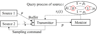
Figure 1: The considered heterogeneous status update system.

To capture the randomness of the wireless link between the transmitter and the monitor, we assume the link is error-prone, i.e., the reception of updates by the monitor are successful with a constant (over slots) probability ${p\in(0,1]}$. Moreover, we assume that at each slot, at most one packet can be transmitted over the link, which stands for the per-slot transmission constraint in the system. Besides, we assume that each transmission occupies one slot, and perfect feedback (i.e., instantaneous and error-free) is available for the link.
Decision Variables: We define two decision variables: one for the scheduling at the transmitter and the other for the sampling decision for Source 2. Let $\alpha_{i}(t)\in\{0,1\}$, $i\in\{1,2\}$, denote the transmission decision of source $i$ at the transmitter in slot $t$, where $\alpha_{i}(t)=1$ means that the transmitter sends the packet of source $i$, and $\alpha_{i}(t)=0$ otherwise. Moreover, let $\beta(t)\in\{0,1\}$ denote the sampling decision of Source 2: $\beta(t)=1$ indicates that the transmitter takes a new sample of Source 2 in slot $t$, and $\beta(t)=0$ otherwise.
Age of Information: First, we make a common assumption (see e.g., [12, 8] and references therein) that the AoI values are upper-bounded by a sufficiently large value $N$. Besides tractability, this accounts for the fact that when the status information becomes excessively stale by reaching $N$, the time-critical end application would not be affected if counting further. Let $\theta_{i}(t)$ be the AoI of source $i$ at the transmitter in slot $t$, and $\delta_{i}(t)$ be the AoI of source $i$ at the monitor in slot $t$. Let $q_{i}(t)\in\{0,1\},\,i\in\{1,2\},$ be an indicator for source $i$, where $q_{i}(t)=1$ means that the packet of source $i$ is transmitted and successfully received in slot $t$, and ${q_{i}(t)=0}$ otherwise.

Assuming that the packet arrivals occur at the beginning of slots, the evolution of the ages for $t=1,2,\dots$, with the initial values $\theta_{i}(0)=0$ and $\delta_{i}(0)=0$, are given as

$$\begin{array}[]{ll}&\theta_{1}(t+1)=\left\{\begin{array}[]{ll}0,&\text{if a packet arrives in $t+1$},\\ \left[\theta_{1}(t)+1\right]^{N},&\text{otherwise},\end{array}\right.\\ &\theta_{2}(t+1)=\left\{\begin{array}[]{ll}0,&\text{if}\leavevmode\nobreak\ \leavevmode\nobreak\ \beta(t+1)=1,\\ \left[\theta_{2}(t)+1\right]^{N},&\text{otherwise}.\end{array}\right.\\ &\delta_{1}(t+1)=\left\{\begin{array}[]{ll}\left[\theta_{1}(t)+1\right]^{N},&\leavevmode\nobreak\ \text{if}\leavevmode\nobreak\ q_{1}(t)=1,\\ \left[\delta_{1}(t)+1\right]^{N},&\leavevmode\nobreak\ \text{otherwise},\end{array}\right.\\ &\delta_{2}(t+1)=\left\{\begin{array}[]{ll}1,&\text{if}\leavevmode\nobreak\ q_{2}(t)=1,\beta(t)=1,\\ \left[\theta_{2}(t)+1\right]^{N},&\text{if}\leavevmode\nobreak\ q_{2}(t)=1,\beta(t)\neq 1,\\ \left[\delta_{2}(t)+1\right]^{N},&\text{otherwise},\end{array}\right.\end{array}$$ (1)

where ${\left[.\right]^{N}}\triangleq\min(.\,,N)$.
We consider that the AoI at the monitor becomes important (only) in the instants when the updates are actually needed/used by the time-critical end application. We capture this by the QAoI [4] by defining a per-source query flag denoted by ${r_{i}(t)\in\{0,1\},\,i\in\{1,2\}},$ where $r_{i}(t)=1$ means that the monitor queries the information of source $i$ in slot $t$, and $r_{i}(t)=0$ otherwise. Accordingly, the QAoI for source $i$ in slot $t$ is defined as $r_{i}(t)\delta_{i}(t)$. We assume that the query flags are generated according to the binary Markov chains, as depicted in Fig. 1, where $\rho_{i}$ and $\bar{\rho}_{i}$ are, respectively, the self-transition probabilities of State $1$ and State $0$.

We denote the sum (discounted) average QAoI at the monitor by $\bar{\delta}$, defined by

$$\begin{array}[]{ll}&\displaystyle\bar{\delta}\triangleq\textstyle\bar{\lambda}\sum_{t=1}^{\infty}{\lambda^{t-1}}\mathbb{E}\left\{\sum_{i}r_{i}(t)\delta_{i}(t)\right\},\end{array}$$ (2)

where $\lambda\in(0,1)$ is the discount factor, $\bar{\lambda}=(1-\lambda)$ is the normalization factor [16, Remark 2.1], and $\mathbb{E}\{\cdot\}$ is the expectation with respect to the random channel, the packet arrival process, and the (possibly random) decision variables $\alpha_{i}(t)$ and $\beta(t)$ made in reaction to the past and current AoI and query values. We also define the (discounted) average number of transmissions, denoted by $\bar{\alpha}$, and the (discounted) average number of sampling actions, denoted by $\bar{\beta}$, as

$$\displaystyle\bar{\alpha}\triangleq\bar{\lambda}\textstyle\sum_{t=1}^{\infty}\lambda^{t-1}\mathbb{E}\left\{\sum_{i}\alpha_{i}(t)\right\},\leavevmode\nobreak\ \displaystyle\bar{\beta}\triangleq\bar{\lambda}\textstyle\sum_{t=1}^{\infty}\lambda^{t-1}\mathbb{E}\left\{\beta(t)\right\}.$$

Our main goal is to solve the following problem:

$$\underset{\{\{\alpha_{i}(t)\}_{i=1}^{2},\beta(t)\}_{t=1,2,\ldots}}{\mbox{minimize}}\leavevmode\nobreak\ \leavevmode\nobreak\ \leavevmode\nobreak\ \bar{\delta}\vspace{-2em}$$ (3a)

subject to $$\bar{\alpha}\leq\Gamma^{\mathrm{tr}},$$ (3b)

$$\bar{\beta}\leq\Gamma^{\mathrm{sm}},$$ (3c)

$$\textstyle\sum_{i}\alpha_{i}(t)\leq 1,\leavevmode\nobreak\ \forall\,t,$$ (3d)

$$\beta(t)\leq\alpha_{2}(t),\leavevmode\nobreak\ \forall\,t,\vspace{-1.2 em}$$ (3e)

with the decision variables ${\{\{\alpha_{i}(t)\}_{i=1}^{2},\beta(t)\}_{t=1,2,\ldots}}$, where ${\Gamma^{\mathrm{tr}}\in(0,1]}$ and ${\Gamma^{\mathrm{sm}}\in(0,1]}$ are limits on the average number of transmissions and sampling actions in the system. The per-slot constraint (3d) limits that at most one packet can be transmitted over the link in each slot. The per-slot constraint (3e) ensures the sampled update in slot $t$ is transmitted at the same slot. Note that constraint (3e) is not obligatory for problem (3), but it eliminates a sub-optimal action, i.e., taking a new sample without its concurrent transmission, which simplifies solving the CMDP problem (introduced next).

Next, we provide an optimal policy to problem (3).

III Optimal Policy

To solve problem (3), we first recast it into a CMDP problem and then (optimally) solve it via solving its equivalent LP [16].

III-A CMDP Formulation of Problem (3)

The CMDP is specified by the following elements:
$\bullet$ State: We define the state in slot $t$ by ${\mathbb{s}(t)\triangleq\big{(}r_{1}(t),\theta_{1}(t),\delta_{1}(t),r_{2}(t),\theta_{2}(t),\delta_{2}(t)\big{)}}$. We denote the state space by $\mathcal{S}$ which is a finite set.
$\bullet$ Action: Actions determine the transmission and sampling decisions while incorporating constraints (3d) and (3e). Thus, we define the action taken in slot $t$ by ${a(t)\in\{0,1,2_{\mathrm{r}},2_{\mathrm{n}}\}}$, where ${a(t)=0}$ means that the transmitter stays idle, ${a(t)=1}$ means that the packet of Source 1 is transmitted/re-transmitted, ${a(t)=2_{\mathrm{r}}}$ means that the packet of Source 2 is re-transmitted, and ${a(t)=2_{\mathrm{n}}}$ means that a new sample of Source 2 is transmitted. Also, $\mathcal{A}$ is the action space of size $|\mathcal{A}|=4$. Actions are determined by a policy $\pi$, which is a (possibly randomized) mapping from $\mathcal{S}$ to $\mathcal{A}$.
$\bullet$ State Transition Probabilities: We denote the state transition probability from state $\mathbb{s}$ to next state $\mathbb{s}^{\prime}$ under an action ${a}$ by $\mathcal{P}_{\mathbb{s}\mathbb{s}^{\prime}}(a)$. Since the evolution of the AoIs in (LABEL:Eq_AoIDy) and the query processes are independent among the sources, the transition probability can be written as ${\mathcal{P}_{\mathbb{s}\mathbb{s}^{\prime}}(a)=\prod_{i}\Pr\{r_{i}^{\prime}\,|\,r_{i}\}\Pr\{\mathbb{\underline{s}}_{i}^{\prime}\,\big{|}\,\mathbb{\underline{s}}_{i},a\}}$, where $\Pr\{r_{i}^{\prime}\,|\,r_{i}\}$ is given by (20), and $\Pr\{\mathbb{\underline{s}}_{i}^{\prime}\,\big{|}\,\mathbb{\underline{s}}_{i},a\}$ is given by (4), in which $\mathbb{\underline{s}}_{i}\triangleq(\theta_{i},\delta_{i})$ contains the current age values, as a part of the current state, associated with source $i$, $\mathbb{\underline{s}}_{i}^{\prime}\triangleq(\theta_{i}^{\prime},\delta^{\prime}_{i})$ contains the next age values, as a part of the next state, associated with source $i$, and $\bar{\mu}=1-\mu$.

$$\Pr\{\mathbb{\underline{s}}_{1}^{\prime}\,\big{|}\,\mathbb{\underline{s}}_{1},a\}=$$ (4)

$$\left\{\begin{array}[]{ll}\mu,&a\neq 1;\leavevmode\nobreak\ \theta^{\prime}_{1}=0,\leavevmode\nobreak\ \delta^{\prime}_{1}=\left[\delta_{1}+1\right]^{N},\\ \bar{\mu},&a\neq 1;\leavevmode\nobreak\ \theta^{\prime}_{1}=\left[\theta_{1}+1\right]^{N},\,\delta^{\prime}_{1}=\left[\delta_{1}+1\right]^{N},\\ \mu p,&a=1;\leavevmode\nobreak\ \theta^{\prime}_{1}=0,\leavevmode\nobreak\ \delta^{\prime}_{1}=\left[\theta_{1}+1\right]^{N},\\ \mu(1-p),&a=1;\leavevmode\nobreak\ \theta^{\prime}_{1}=0,\leavevmode\nobreak\ \delta^{\prime}_{1}=\left[\delta_{1}+1\right]^{N},\\ \bar{\mu}p,&a=1;\leavevmode\nobreak\ \theta^{\prime}_{1}=\left[\theta_{1}+1\right]^{N},\leavevmode\nobreak\ \delta^{\prime}_{1}=\left[\theta_{1}+1\right]^{N},\\ \bar{\mu}(1-p),&a=1;\leavevmode\nobreak\ \theta^{\prime}_{1}=\left[\theta_{1}+1\right]^{N},\leavevmode\nobreak\ \delta^{\prime}_{1}=\left[\delta_{1}+1\right]^{N},\\ 0&\text{otherwise}.\end{array}\right.$$ (12)

$$\Pr\{\mathbb{\underline{s}}_{2}^{\prime}\leavevmode\nobreak\ \big{|}\leavevmode\nobreak\ \mathbb{\underline{s}}_{2},a\}=$$

$$\left\{\begin{array}[]{ll}1,&a\neq\{2_{\mathrm{r}},2_{\mathrm{n}}\};\,\theta^{\prime}_{2}=\left[\theta_{2}+1\right]^{N},\,\delta^{\prime}_{2}=\left[\delta_{2}+1\right]^{N},\\ p,&a=2_{\mathrm{r}};\leavevmode\nobreak\ \theta^{\prime}_{2}=\left[\theta_{2}+1\right]^{N},\leavevmode\nobreak\ \delta^{\prime}_{2}=\left[\theta_{2}+1\right]^{N},\\ 1-p,&a=2_{\mathrm{r}};\leavevmode\nobreak\ \theta^{\prime}_{2}=\left[\theta_{2}+1\right]^{N},\leavevmode\nobreak\ \delta^{\prime}_{2}=\left[\delta_{2}+1\right]^{N},\\ p,&a=2_{\mathrm{n}};\leavevmode\nobreak\ \theta^{\prime}_{2}=1,\leavevmode\nobreak\ \delta^{\prime}_{2}=1,\\ 1-p,&a=2_{\mathrm{n}};\leavevmode\nobreak\ \theta^{\prime}_{2}=1,\leavevmode\nobreak\ \delta^{\prime}_{2}=\left[\delta_{2}+1\right]^{N},\\ 0&\text{otherwise}.\end{array}\right.$$ (19)

$$\Pr\{r_{i}^{\prime}\,|\,r_{i}\}=\left\{\begin{array}[]{ll}\rho_{i},&r_{i}=1;\leavevmode\nobreak\ r^{\prime}_{i}=1,\\ 1-\rho_{i},&r_{i}=1;\leavevmode\nobreak\ r^{\prime}_{i}=0,\\ \bar{\rho}_{i},&r_{i}=0;\leavevmode\nobreak\ r^{\prime}_{i}=0,\\ 1-\bar{\rho}_{i},&r_{i}=0;\leavevmode\nobreak\ r^{\prime}_{i}=1.\end{array}\right.$$ (20)

$\bullet$ Cost Functions: The cost functions include: 1) the QAoI cost defined by $c(\mathbb{s}(t))=\sum_{i}r_{i}(t)\delta_{i}(t)$, 2) the transmission cost defined by $d^{\mathrm{tr}}(a(t))=\mathds{1}_{\{a\neq 0\}}$, and 3) the sampling cost defined by $d^{\mathrm{sm}}(a(t))=\mathds{1}_{\{a=2_{\mathrm{n}}\}}$, where $\mathds{1}_{\{\cdot\}}$ is an indicator function which equals to $1$ when the condition in $\{\cdot\}$ holds.
By the above definitions, problem (3) can be recast as the following CMDP problem

$$\underset{\pi\in\Pi}{\text{minimize}}\leavevmode\nobreak\ \bar{\lambda}\textstyle\sum_{t=1}^{\infty}\lambda^{t-1}\mathbb{E}^{\pi,\eta}\left\{c(\mathbb{s}(t))\right\},$$ (21a)

subject to $$\bar{\lambda}\textstyle\sum_{t=1}^{\infty}\lambda^{t-1}\mathbb{E}^{\pi,\eta}\left\{d^{\mathrm{tr}}(a(t))\right\}\leq\Gamma^{\mathrm{tr}},$$ (21b)

$$\bar{\lambda}\textstyle\sum_{t=1}^{\infty}\lambda^{t-1}\mathbb{E}^{\pi,\eta}\left\{d^{\mathrm{sm}}(a(t))\right\}\leq\Gamma^{\mathrm{sm}},$$ (21c)

where $\Pi$ is the set of all stationary randomized policies, and $\mathbb{E}^{\pi,\eta}$ denotes the expectation when following a policy $\pi$ for a given initial distribution (over the state space) $\eta$.
Next, we provide an optimal policy to problem (21).

III-B Linear Programming of the CMDP Problem (21)

Here, we transform problem (21) into an LP. For a notional simplicity, we denote state $\mathbb{s}$ by $s$. Let ${x(s,a)\in\mathbb{R}^{|\mathcal{S}||\mathcal{A}|}}$, ${\forall\,s\in\mathcal{S},\leavevmode\nobreak\ \forall\,a\in\mathcal{A}}$, be defined as [16, Ch. 3]

$$\begin{array}[]{ll}x(s,a)\triangleq\bar{\lambda}\sum_{t=1}^{\infty}\lambda^{t-1}\Pr^{\eta}{\{s(t)=s,\,a(t)=a\}},\end{array}$$ (23)

where $\Pr^{\eta}{\{s(t)=s,\,a(t)=a\}}$ denotes the probability of taking action $a$ at state $s$ in slot $t$ given the initial distribution $\eta$. It is noteworthy that $x(s,a),\leavevmode\nobreak\ \forall\,s\in\mathcal{S},\leavevmode\nobreak\ \forall\,a\in\mathcal{A},$ can be interpreted as the long run discounted time that the system is in state $s$ and action $a$ is chosen. Then, the CMDP problem (21) can be transformed into the following LP [16, Ch. 3]:

$$\underset{\mathbb{X}}{\text{minimize}}\leavevmode\nobreak\ \leavevmode\nobreak\ \textstyle\sum_{s\in\mathcal{S}}\sum_{a\in\mathcal{A}}x(s,a)c(s)$$ (24a)

subject to $$\textstyle\sum_{s\in\mathcal{S}}\sum_{a\in\mathcal{A}}x(s,a)d^{\mathrm{tr}}(a)\leq\Gamma^{\mathrm{tr}},$$ (24b)

$$\textstyle\sum_{s\in\mathcal{S}}\sum_{a\in\mathcal{A}}x(s,a)d^{\mathrm{sm}}(a)\leq\Gamma^{\mathrm{sm}},$$ (24c)

$$\textstyle\sum_{s^{\prime}\in\mathcal{S}}\sum_{a\in\mathcal{A}}x(s^{\prime},a)\big{(}\mathds{1}_{\{s=s^{\prime}\}}-\lambda\mathcal{P}_{s^{\prime}s}(a)\big{)}$$

$$=\bar{\lambda}\eta(s),\forall\,s\in\mathcal{S},$$ (24d)

$$x(s,a)\geq 0,\leavevmode\nobreak\ \forall\,s\in\mathcal{S},\leavevmode\nobreak\ \forall\,a\in\mathcal{A},$$ (24e)

with variables $\mathbb{X}=[x(s,a)]$, where $\eta(s),\,\forall\,s\in\mathcal{S}$, is the probability that the initial state is state $s$.

By [16, Theorem 3.3], the following theorem relates a solution of the LP (24) to a solution of problem (21).

Theorem 1.

First, the optimal value of the CMDP problem (21) equals to the optimal value of the LP (24). Moreover, let ${\mathbb{X}^{*}=[x^{*}(s,a)]},$ be a solution of the LP (24). Then, a stationary randomized policy $\pi\triangleq\{f(s,a)\}$ with

$$\begin{array}[]{cc}f(s,a)=\left\{\begin{array}[]{ll}x^{*}(s,a)/\bar{x}_{s},&\text{if}\leavevmode\nobreak\ \bar{x}_{s}>0,\\ \text{arbitrary},&\text{otherwise},\end{array}\right.\end{array}$$ (28)

is an optimal policy to the CMDP problem (21), where ${\bar{x}_{s}=\textstyle\sum_{a^{\prime}\in\mathcal{A}}x^{*}(s,a^{\prime})}$, and $f(s,a),\leavevmode\nobreak\ \forall\,s\in\mathcal{S},\leavevmode\nobreak\ \forall\,a\in\mathcal{A},$ is the probability that an action $a$ is chosen at state $s$.

Complexity analysis: The complexity of finding the optimal policy (determined by (28)) comes from the complexity of the LP (24), which is exponential in the number of sources. This is because its number of variables and constraints vary with the state space size of the CMDP problem (21), which grows exponentially with the number of sources. Thus, the optimal policy becomes computationally inefficient when applied for large numbers of sources. To strike a balance between the performance and complexity, a heuristic low-complexity policy is provided in the next section.

IV Low-Complexity Policy

In this section, we develop a low-complexity policy to the main problem (3) via the following procedure: 1) we relax the per-slot transmission constraint (3d), 2) transform the relaxed problem to a weakly coupled CMDP problem which is then solved by its equivalent LP [5], and 3) propose a dynamic truncation algorithm to satisfy the transmission constraint (3d).
We relax the per-slot constraint (3d) to the (discounted) time average constraint $\bar{\lambda}\sum_{t=1}^{\infty}\lambda^{t-1}\mathbb{E}\{\textstyle\sum_{i}\alpha_{i}(t)\}\leq 1$. This constraint then becomes inactive due to constraint (3b). Then, the main problem (3) without constraint (3d) can be cast as a weakly coupled CMDP problem. This is because the transition probabilities, the action space, and the immediate cost functions become independent among the sources; now, the average transmission constraint (3b) is the only constraint coupling the sources.
To proceed, we define the state, action, transition probabilities, and cost functions associated with each source $i$. The state of source $i$ in slot $t$ is ${s_{i}(t)\triangleq\big{(}r_{i}(t),\theta_{i}(t),\delta_{i}(t)\big{)}}$, with state space $\mathcal{S}_{i}$, which is a finite set. The action of source $i$ in slot $t$ is denoted by $a_{i}(t)\in\mathcal{A}_{i}$ with action spaces $\mathcal{A}_{1}=\{0,1\}$ and $\mathcal{A}_{2}=\{0,2_{\mathrm{r}},2_{\mathrm{n}}\}$. The state transition probabilities of source $i$, denoted as ${\mathcal{\tilde{P}}_{s_{i}s_{i}^{\prime}}^{i}(a),\leavevmode\nobreak\ \forall\,s_{i},\,s_{i}^{\prime}\in\mathcal{S}_{i}}$, is given by $\Pr\{r_{i}^{\prime}\,|\,r_{i}\}\Pr\{\mathbb{\underline{s}}_{i}^{\prime}\,\big{|}\,\mathbb{\underline{s}}_{i},a\}$, where $\Pr\{r_{i}^{\prime}\,|\,r_{i}\}$ and $\Pr\{\mathbb{\underline{s}}_{i}^{\prime}\,\big{|}\,\mathbb{\underline{s}}_{i},a\}$ were defined in (20) and (4). The QAoI cost of source $i$ is ${c_{i}({s}_{i}(t))=r_{i}(t)\delta_{i}(t)}$. The transmission cost of source $i$ is ${d_{i}^{\mathrm{tr}}(a_{i}(t))=\mathds{1}_{\{a_{i}(t)\neq 0\}}}$. The sampling cost of Source 2 is ${d^{\mathrm{sm}}(a_{2}(t))=\mathds{1}_{\{a_{2}(t)=2_{n}\}}}$.
First, for a presentation simplicity, we remove the subscript $i$ from $s_{i}(t)$ and $a_{i}(t)$. Then, for each source $i\in\{1,2\}$, let $x_{i}(s,a)\in\mathbb{R}^{|\mathcal{S}_{i}||\mathcal{A}_{i}|},\leavevmode\nobreak\ \forall\,s\in\mathcal{S}_{i},\leavevmode\nobreak\ \forall\,a\in\mathcal{A}_{i},$ be defined as

$$\begin{array}[]{ll}x_{i}(s,a)&\triangleq\bar{\lambda}\sum_{t=1}^{\infty}\lambda^{t-1}\Pr_{i}^{\eta_{i}}{\{s(t)=s,\,a(t)=a\}},\end{array}$$

where $\Pr_{i}^{\eta_{i}}{\{s(t)=s,\,a(t)=a\}}$ denotes the probability of taking action $a\in\mathcal{A}_{i}$ at state $s\in\mathcal{S}_{i}$ in slot $t$ given the initial distribution $\eta_{i}$. Then, the corresponding LP of the weakly coupled CMDP problem is given by

$$\underset{\mathbb{X}_{i}}{\mbox{minimize}}\leavevmode\nobreak\ \leavevmode\nobreak\ \textstyle\sum_{i}\textstyle\sum_{s\in\mathcal{S}_{i}}\sum_{a\in\mathcal{A}_{i}}x_{i}(s,a)c_{i}(s)$$ (29a)

subject to $$\textstyle\sum_{i}\textstyle\sum_{s\in\mathcal{S}_{i}}\sum_{a\in\mathcal{A}_{i}}x_{i}(s,a)d_{i}^{\mathrm{tr}}(a)\leq\Gamma^{\mathrm{tr}},$$ (29b)

$$\textstyle\sum_{s\in\mathcal{S}_{2}}\sum_{a\in\mathcal{A}_{2}}x_{2}(s,a)d^{\mathrm{sm}}(a)\leq\Gamma^{\mathrm{sm}},$$ (29c)

$$\textstyle\sum_{s^{\prime}\in\mathcal{S}_{i}}\sum_{a\in\mathcal{A}_{i}}x_{i}(s^{\prime},a)\big{(}\mathds{1}_{\{s=s^{\prime}\}}-\lambda\mathcal{\tilde{P}}^{i}_{s^{\prime}s}(a)\big{)}$$

$$=\bar{\lambda}\eta_{i}(s),\forall\,i,\leavevmode\nobreak\ \forall\,s\in\mathcal{S}_{i},$$ (29d)

$$x_{i}(s,a)\geq 0,\forall\,i,\leavevmode\nobreak\ \forall\,s\in\mathcal{S}_{i},\leavevmode\nobreak\ \forall\,a\in\mathcal{A}_{i},$$ (29e)

with variables $\mathbb{X}_{i}=[x_{i}(s,a)],\leavevmode\nobreak\ i\in\{1,2\}$.

Let $\mathbb{X}_{i}^{*}=[x_{i}^{*}(s,a)]$ be a solution of the LP (29). By results of [5], an optimal stationary randomized policy for each source $i$, $\pi^{*}_{i}\triangleq\{f_{i}(s,a)\}$, is given by

$$\begin{array}[]{cc}f_{i}(s,a)=\left\{\begin{array}[]{ll}x_{i}^{*}(s,a)/\bar{x}_{i,s},&\text{if}\leavevmode\nobreak\ \bar{x}_{i,s}>0,\\ \text{arbitrary},&\text{otherwise},\end{array}\right.\end{array}$$ (30)

where ${\bar{x}_{i,s}=\textstyle\sum_{a^{\prime}\in\mathcal{A}_{i}}x_{i}^{*}(s,a^{\prime})}$ and ${f_{i}(s,a)}$, ${\forall\,s\in\mathcal{S}_{i}}$, ${\forall\,a\in\mathcal{A}_{i}}$, is the probability that an action $a\in\mathcal{A}_{i}$ is chosen at state $s\in\mathcal{S}_{i}$ for source $i$. Notably, the per-source policies $\{\pi_{i}^{*}\}$ construct a lower-bound policy to the main problem (3); this lower bound is tight as empirically shown in Fig. 4.
Having constructed the above weakly coupled CMDP and derived its solution, we now propose a near-optimal low-complexity policy for the main problem (3) that operates as follows: (i) it determines an action of each source $i$ in each slot $t$ according to $\pi^{*}_{i}$, and (ii) having the actions determined, if there is more than one packet to be transmitted, the packet of source $\underline{i}$ will be transmitted, where ${\underline{i}=\operatorname*{arg\,max}_{i\in\{1,2\}}\{h_{i}(t)\}}$ in which $h_{1}(t)$ and $h_{2}(t)$ are given as

$$\begin{array}[]{cc}h_{1}(t)\triangleq r_{1}(t)(\delta_{1}(t)-\theta_{1}(t)),\leavevmode\nobreak\ h_{2}(t)\triangleq r_{2}(t)\delta_{2}(t).\end{array}$$ (32)

We term the above Step (ii) as a dynamic truncation algorithm, which still couples the sources. The main idea of the truncation algorithm is to transmit the packet that is more fresh from the monitor’s perspective, as it has greater potential to decrease the AoI at the monitor. To capture such relative freshness, we have used the AoI difference between the monitor and the transmitter for Source 1, and the AoI at the monitor itself for Source 2.

Complexity analysis: The main complexity of finding the low-complexity policy comes from solving the LP (29), which is (only) linear in the number of sources. This is because its number of variables and constraints vary with the state space size of the weakly-coupled CMDP problem, which grows linearly with the number of sources. Thus, the proposed policy has low complexity, and as numerically shown in the next section, obtains near-optimal performance.

V Numerical Results

Here, we assess the performance of the proposed policies. We set $N=20$, $\rho_{1}=\rho_{2}=0.7$, $\bar{\rho}_{1}=\bar{\rho}_{2}=0.4$, and $\lambda=0.99999$, and initialize the query flags by the steady-state probabilities of the Markov chains, unless otherwise stated. For a benchmark, we consider a greedy-based baseline policy with the decision rule: If $\bar{D}^{\mathrm{tr}}(t)\leq\Gamma^{\mathrm{tr}}$, find ${\underline{i}=\operatorname*{arg\,max}_{i\in\{1,2\}}\{h_{i}(t)\}}$; otherwise, $a(t)=0$. If $\underline{i}=1$, then $a(t)=1$; otherwise, do the following. If $\bar{D}^{\mathrm{sm}}(t)\leq\Gamma^{\mathrm{sm}}$, then $a(t)=2_{\mathrm{n}}$; otherwise, $a(t)=2_{\mathrm{r}}$. Here, $\bar{D}^{\mathrm{tr}}(t)$ and $\bar{D}^{\mathrm{sm}}(t)$ denote, respectively, the discounted average number of transmissions and sampling actions until slot $t$, and $h_{i}(t)$ was given by (32).
Fig. 2 shows the sum (discounted) average QAoI performance of the proposed policies and the baseline policy as a function of the transmission budget $\Gamma^{\mathrm{tr}}$ (i.e., the limit on the average number of transmissions). First, Fig. 2 (as well as Fig. 3) reveals that the heuristic policy has near-optimal performance, i.e., it nearly coincides with the optimal policy. The figure shows the importance of an optimal trade-off design between freshness and resource usage, as the performance gap between the baseline policy and the proposed policies is significant when the transmission budget is small. Moreover, the figure reveals that the QAoI is more sensitive to the transmission budget than the sampling budget, as expected.
Fig. 3 examines the impact of the channel reliability $p$ on the sum average QAoI performance of the different policies for different packet arrival rate $\mu$ for Source 1. First, the figure shows that the performance gap between the proposed policies and the baseline policy is large, especially when the channel reliability is small. The figure also shows that the QAoI considerably decreases as the channel reliability increases because it increases the chance that the monitor receives updates more frequently. Moreover, it can be seen that the QAoI would not change much by increasing the arrival rate under a good channel condition.

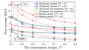
Figure 2: The sum (discounted) average QAoI versus the transmission budget $\Gamma^{\mathrm{tr}}$ for different channel reliabilities $p$, where $\mu=0.6$.

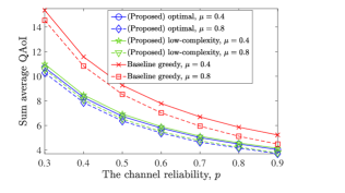
Figure 3: The sum (discounted) average QAoI versus the channel reliability $p$, where $\Gamma^{\mathrm{tr}}=0.5$ and $\Gamma^{\mathrm{sm}}=0.3$.

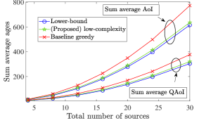
Figure 4: The sum (discounted) average AoI and QAoI versus the total number of sources with equal number of random arrival and generate-at-will sources, where $N=150$, $\Gamma^{\mathrm{tr}}=0.8$, $\Gamma^{\mathrm{sm}}=0.3$, and $p=0.99999$. Moreover, $\mu_{i}=0.5$ (for all the random arrival sources) and $\rho_{i}=\bar{\rho}_{i}=0.7$ (for all sources).

Fig. 4 shows the impact of the number of sources on the sum average QAoI/AoI performance of different policies. First, the figure shows that the proposed low-complexity policy indeed preserves near-optimal performance in a general multi-source setup, as it nearly coincides with the lower-bound policy. Moreover, the performance gap between the baseline policy and the proposed policy increases in the number of sources.

VI Conclusion

We provided a query-age-optimal joint sampling and scheduling policy for a heterogeneous status update system under average sampling, average transmission, and per-slot transmission constraints. To this end, a CMDP problem with two average constraints was cast and solved via its equivalent LP. We also provided a low-complexity policy by casting a weakly-coupled CMDP problem and solving it via its equivalent LP. Numerical results showed the effectiveness of the proposed policies, revealing that age-optimal sampling and scheduling is crucial for resource-constrained status update systems, where a greedy-based policy is inefficient. Moreover, the near-optimal performance of the proposed low-complexity policy substantiates that the LP approach provides a viable solution for practical systems having many sources/sensors.

References

- [1] S. Kaul, R. Yates, and M. Gruteser, “Real-time status: How often should one update?,” in Proc. IEEE Int. Conf. on Computer Commun., pp. 2731–2735, Orlando, FL, USA, Mar. 2012.
- [2] Y. Sun, I. Kadota, R. Talak, and E. Modiano, “Age of information: A new metric for information freshness,” Synthesis Lectures on Communication Networks, vol. 12, no. 2, pp. 1–224, Dec. 2019.
- [3] A. Maatouk, M. Assaad, and A. Ephremides, “On the age of information in a csma environment,” IEEE/ACM Trans. Netw., vol. 28, no. 2, pp. 818–831, Apr. 2020.
- [4] F. ChiarIoTti, J. Holm, A. E. Kalør, B. Soret, S. K. Jensen, T. B. Pedersen, and P. Popovski, “Query age of information: Freshness in pull-based communication,” IEEE Trans. Commun., vol. 70, no. 3, pp. 1606–1622, Mar. 2022.
- [5] M. Gagrani and A. Nayyar, “Weakly coupled constrained markov decision processes in borel spaces,” in Proc. American Control Conf., pp. 2790–2795, Denver, CO, USA, Jul. 2020.
- [6] Y. Cao, Y. Teng, M. Song, and N. Wang, “Age-driven joint sampling and non-slot based scheduling for industrial internet of things,” arXiv preprint arXiv:2205.04092, May, 2022.
- [7] E. T. Ceran, D. Gündüz, and A. György, “Average age of information with hybrid ARQ under a resource constraint,” IEEE Trans. Wireless Commun., vol. 18, no. 3, pp. 1900–1913, Mar. 2019.
- [8] E. Fountoulakis, M. Codreanu, A. Ephremides, and N. Pappas, “Joint sampling and transmission policies for minimizing cost under AoI constraints,” arXiv preprint arXiv:2103.15450,, Mar. 2021.
- [9] J. Pan, A. M. Bedewy, Y. Sun, and N. B. Shroff, “Optimizing sampling for data freshness: Unreliable transmissions with random two-way delay,” arXiv preprint arXiv:2201.02929, 2022.
- [10] A. M. Bedewy, Y. Sun, S. Kompella, and N. B. Shroff, “Optimal sampling and scheduling for timely status updates in multi-source networks,” IEEE Trans. Inf. Theory, vol. 67, no. 6, pp. 4019–4034, Jun. 2021.
- [11] I. Kadota, A. Sinha, E. Uysal-Biyikoglu, R. Singh, and E. Modiano, “Scheduling policies for minimizing age of information in broadcast wireless networks,” IEEE/ACM Trans. Netw., vol. 26, no. 6, pp. 2637–2650, Dec. 2018.
- [12] B. Zhou and W. Saad, “Joint status sampling and updating for minimizing age of information in the internet of things,” IEEE Trans. Commun., vol. 67, no. 11, pp. 7468–7482, Nov. 2019.
- [13] S. Wang, M. Chen, Z. Yang, C. Yin, W. Saad, S. Cui, and H. V. Poor, “Distributed reinforcement learning for age of information minimization in real-time IoT systems,” IEEE J. Sel. Topics Signal Process., vol. 16, no. 3, pp. 501–515, Apr. 2022.
- [14] F. Li, Y. Sang, Z. Liu, B. Li, H. Wu, and B. Ji, “Waiting but not aging: Optimizing information freshness under the pull model,” IEEE/ACM Trans. Netw., vol. 29, no. 1, pp. 465–478, Feb. 2021.
- [15] M. E. Ildiz, O. T. Yavascan, E. Uysal, and O. T. Kartal, “Pull or wait: How to optimize query age of information,” arXiv preprint arXiv:2111.02309, Nov. 2021.
- [16] E. Altman, Constrained Markov Decision Processes. volume 7. CRC Press, 1999.
- [17] M. L. Puterman, Markov Decision Processes: Discrete Stochastic Dynamic Programming. The MIT Press, 1994.
- [18] L. Kallenberg, Markov decision processes. Lect. Notes. Univ. Leiden, Oct. 2016.