Anomaly Detection on Financial Time Series by Principal Component Analysis and Neural Networks

Abstract

A major concern when dealing with financial time series involving a wide variety of market risk factors is the presence of anomalies. These induce a miscalibration of the models used to quantify and manage risk, resulting in potential erroneous risk measures. We propose an approach that aims at improving anomaly detection on financial time series, overcoming most of the inherent difficulties. Valuable features are extracted from the time series by compressing and reconstructing the data through principal component analysis. We then define an anomaly score using a feedforward neural network. A time series is considered to be contaminated when its anomaly score exceeds a given cut-off value. This cutoff value is not a hand-set parameter, but rather calibrated as a neural network parameter, throughout the minimization of a customized loss function. The efficiency of the proposed approach compared to several well-known anomaly detection algorithms is numerically demonstrated on both synthetic and real data sets, with high and stable performance being achieved with the PCA NN approach. We show that value-at-risk estimation errors are reduced when the proposed anomaly detection model is used with a basic imputation approach to correct the anomaly.

Key words: anomaly detection, financial time series, principal component analysis, neural network, missing data, market risk, value at risk.

1 Introduction

In the context of financial risk management, financial risk models are of utmost importance in order to quantify and manage financial risk. Their outputs, risk measurements, can both help in the process of decision making and ensure that the regulatory requirements are met (Basel Committee on Banking Supervision, 2013). Financial management thus heavily relies on financial risk models and the interpretation of their outputs. The data usually consist of time series representing a wide variety of market risk factors. A major issue of such data is the presence of anomalies. A value of the time series is considered to be abnormal whenever its behaviour is significantly different from the behaviour of the rest of the time series (Hawkins, 1980). In this work, we focus on the detection of abnormal observations in a market risk factor time series used to calibrate financial risk models. Indeed, erroneous input data may wrongly impact the calibrated model parameters. A typical example is the estimation of the covariance matrix of a bank market risk factors. This covariance matrix is involved in the computation of value-at risks (VaR) or expected shortfalls (expected losses above the VaR level). Since the true covariance is unknown, it has to be estimated from the data. However, the presence of anomalies in the data might have an impact on this estimation. For this specific case, robust methods, less sensitive to anomalies, can be used. Yet, existing robust estimators are computationally expensive, with a polynomial or even exponential time complexity in terms of the number of market risk factors. A faster approach was suggested by Cheng et al. (2019), but this algorithm only applies to the estimation of the covariance matrix in the case of Gaussian distribution. Financial risk models used by banks are widespread and various. Therefore, instead of seeking for a robust version for each of them, we propose to detect anomalies directly on the time series.

Contributions of the Paper

Our PCA NN methodology identifies anomalies on time series using a principal component analysis (PCA) and neural networks (NN) as underlying models. This methodology overcomes common pitfalls associated with anomaly detection. PCA is first used as a features extractor on (augmented if needed) data. Anomaly detection is then performed in two steps. The first step identifies the time series with anomalies evaluating the propensity of the time series to be contaminated, as reflected by its so-called anomaly score. Toward this end, we calibrate a feedforward neural network through the minimization of a customized loss. This customized loss allows us to calibrate the cut-off value on the anomaly scores, without resorting to expert judgement. In this way, we remove the expert bias. The second step localizes the anomaly among the observed values of the identified contaminated time series.

Outline

The PCA NN approach is detailed in Section 2. Section 3 describes the methodology used for generating the data on which our approach is thoroughly tested in Sections 4, 5 and 6, exploiting the knowledge of the data generating process for benchmarking purposes. Section 7 illustrates the benefit of using our approach as a data cleaning preprocessing stage on a downstream task, namely value-at-risk computations. This is completed by further numerical experiments on real data sets in Section 8. Section 9 concludes. Section A and B provide reviews of the anomaly detection literature and algorithms. Section C addresses the data stationarity issue.

2 The PCA NN Anomaly Detection Approach

2.1 Notations

Let

$$\bm{X}=\left(X^{1},X^{2},\ldots,X^{i},\ldots,X^{n}\right)^{\top},$$ (1)

where the column-vector $X^{i}=\left(x_{t_{1}}^{i},x_{t_{2}}^{i},\ldots,x_{t_{j}}^{i}\ldots,x_{t_{p}}^{i}\right)\in\mathbb{R}^{p}$ corresponds to the $i$-th observed time series, and $x_{t_{j}}^{i}$ to the value observed at time $t_{j}$ in the $i$-th time series.

Our method fits into the supervised framework. We thus assume that the data matrix $\bm{X}$ comes along with two label vectors. The first label vector $\bm{A}=\left(A^{1},\ldots,A^{n}\right)\in\{0,1\}^{n}$ identifies the time series containing anomalies referred to as contaminated time series. For $i=1,\ldots,n$, we define the identification labels as

$$A^{i}=\begin{cases}1&\text{if there exists $j$ such that $x^{i}_{t_{j}}$ is an anomaly}.\\ 0&\text{otherwise.}\end{cases}$$ (2)

The second label vector $\bm{L}$ concerns solely the contaminated time series. Its coefficients correspond to the localization labels, i.e. time stamps at which an anomaly occurs. For $j=1,\ldots,p$ and $i\in I_{c}=\{i:A^{i}=1\}$ (the set of contaminated time series),

$$L^{i}=\jmath\quad\text{ when the anomaly occurs at time $t_{\jmath}$ for the $i$-th contaminated time series},$$

$\bm{X},\bm{A}$ and $\bm{L}$ are general notations. As the model involves a learning phase, we denote by $\bm{X}^{Train}$, $\bm{A}^{Train}$ and $\bm{L}^{Train}$ the data used for calibration and, by $\bm{X}^{Test}$, $\bm{A}^{Test}$ and $\bm{L}^{Test}$ the independent data sets on which the model performance is evaluated.

2.2 Methodology Overview

The anomaly detection model we propose is a two step supervised-learning approach. The contaminated time series identification step aims at identifying among the observed time series the ones with potential anomalies. The anomaly localization step consists in finding the location of the anomaly in each contaminated time series identified during the first step.

The model used in the first step falls under the scope of binary classification models, assigning to each time series a predicted label

$$\widehat{A}^{i}=\begin{cases}1&\text{if $X^{i}$ is considered as contaminated by the identification model.}\\ 0&\text{otherwise.}\end{cases}$$

The second step uses a multi-classification model. For each contaminated time series identified in the first step, the model predicts a unique time stamp $\widehat{L}^{i}$ at which the anomaly has occurred. Formally, the observed value at the time stamp $t_{\hat{\jmath}^{i}}$ of the $i$-th contaminated time series is considered abnormal, meaning that the observation $x^{i}_{t_{\hat{\jmath}^{i}}}$ is abnormal. Thus,

$$\widehat{L}^{i}=\hat{\jmath}^{i}\quad\text{ with }\quad\hat{\jmath}^{i}\in\{1,\dots,p\}.$$

Our two-step anomaly detection model localizes only one anomaly per run, if any. Several iterations allow removing all anomalies. Indeed, as long as the time series is identified as contaminated, by the first step of the method, the time series can go through the second step. Once all anomalies have been localized the final stage of the approach is to remove the abnormal values and suggest imputation values (see Section 6.1).

2.3 Theoretical Basics of Principal Component Analysis

A fundamental intuition behind our anomaly detection algorithm is the existence of a lower dimensional subspace where normal and abnormal observations are easily distinguishable. Since the selected principal components explain a given level of the variance of the data, they represent the common and essential characteristics to all observations. As one might reasonably expect, these characteristics mostly represent the normal observations. When the inverse transformation is applied, the model successfully reconstructs the normal observations with the help of the extracted characteristics, while it fails into reconstructing the anomalies.

In this section, we recall the theoretical tenets of the principal component analysis (PCA) useful for our purpose. The idea of PCA is to project the data from the observation space of dimension $p$ into a latent space of dimension $k$, with $k<p$. This latent space is generated by the $k$ directions for which the variance retained under projection is maximal.

The first principal component $U$ is given by $U=w^{\top}\bm{X},$ where $w$ is a to-be-determined vector of weights. Since the PCA aims at maximizing the variance along its principal components, $w$ is sought for as

$$\arg\max_{\|w\|=1}w^{\top}\Sigma w\,,$$

where $\Sigma$ is the covariance matrix of $\bm{X}$. The optimal solution by the Lagrangian method is given by $\Sigma w=\lambda w\,$, where $\lambda>0$ is a Lagrangian multiplier. Multiplying both sides by $w^{\top}$ results in $w^{\top}\Sigma w=\lambda$. Following the same process with an additional constraint regarding the orthogonality between the principal components, one can show that the $k$ first principal components correspond to the eigenvectors associated with the $k$ dominant eigenvalues of $\Sigma$.

The transfer matrix $\Omega_{\bm{X}}\in\mathbb{R}^{k\times p}$ is defined by the eigenvectors of $\Sigma$ associated with its $k$ largest eigenvalues. This transfer matrix $\Omega_{\bm{X}}$ applied to any observation in the original observation space projects it into the latent space. Since the transformation is linear, reconstructing the initial observations from their equivalent in the latent space is straightforward. Using PCA on the data matrix $\bm{X}$, the transfer matrix $\Omega_{\bm{X}}$ can be inferred. The projection of the observations into the latent space $\bm{Z}\in\mathbb{R}^{n\times k}$ is then given by $\bm{Z}=\bm{X}\Omega_{\bm{X}}^{\top}$, while their reconstructed values are given by $\widehat{\bm{X}}=\bm{Z}\Omega_{\bm{X}}$.

The reconstruction errors $\varepsilon^{i}$ for each time series defined by

$$\varepsilon^{i}=\widehat{X}^{i}-X^{i},\quad i=1,\ldots,n,$$ (3)

referred in the sequel as the new features, are our new representation of data, given as inputs to our models. Algorithm 1 summarizes how to compute these reconstruction errors. The two steps of the model use the same inputs, namely these reconstruction errors. Nevertheless, the processing these inputs undergo in each step differs.

inputs : number of principal components $k$

out of sample data $\bm{X}^{Test}$

training data if not trained yet $\bm{X}^{Train}$

if not trained yet then

       $\Omega_{\bm{X}^{Train}}\leftarrow\mathrm{PCA}(\bm{X}^{Train},k)$;

      

end if

$\bm{\varepsilon}^{Train}=\bm{X}^{Train}\left(\Omega_{\bm{X}^{Train}}^{\top}\Omega_{\bm{X}^{Train}}-I_{p}\right)$

$\bm{\varepsilon}^{Test}=\bm{X}^{Test}\left(\Omega_{\bm{X}^{Train}}^{\top}\Omega_{\bm{X}^{Train}}-I_{p}\right)$

outputs : $\bm{\varepsilon}^{Train}$ reconstruction errors for the train set

$\bm{\varepsilon}^{Test}$ reconstruction errors for the test set

Algorithm 1 Features extraction with PCA

2.4 Contaminated Time Series Identification

The first step of the approach aims at identifying the time series with anomalies based on the reconstruction errors obtained using PCA and Algorithm 1. In this section, we detail the process these new features undergo. We assign to each reconstruction error an anomaly score which computation is handled by a neural network (NN) (see Goodfellow et al., 2016). We also numerically demonstrate that our NN has an advantage over a naive approach in terms of being able to assess more accurately the propensity of a time series of being contaminated.

Naive approach

A naive and natural approach to define the anomaly score is to consider the $\ell^{2}$-norm of the reconstruction errors $\widetilde{\varepsilon}_{i}=\lVert\varepsilon^{i}\rVert_{2}$, $i=1,\ldots,n$. This anomaly score represents the propensity of a time series to be contaminated or not. The scores are first split into two sets depending on whether the corresponding time series is contaminated or not. We denote by $\widetilde{\bm{\varepsilon}}^{c}$ and $\widetilde{\bm{\varepsilon}}^{u}$ the set of contaminated and uncontaminated time series anomaly scores, i.e.

$$\widetilde{\bm{\varepsilon}}^{c} :=\{\lVert\varepsilon^{i}\rVert_{2};\;A^{i}=1\,\}=\{\widetilde{\varepsilon}_{i},\,i\in I_{c}\}$$

$$\widetilde{\bm{\varepsilon}}^{u} :=\{\lVert\varepsilon^{i}\rVert_{2};\;A^{i}=0\,\}=\{\widetilde{\varepsilon}_{i},\,i\notin I_{c}\}.$$

The density distribution function of each class of time series $f^{u}$ and $f^{c}$, i.e. for both $\widetilde{\bm{\varepsilon}}^{c}$ and $\widetilde{\bm{\varepsilon}}^{u}$, is then estimated using kernel density estimation (Węglarczyk, 2018). For $l=\{c,u\}$, let $\bm{\varepsilon}^{l}$ be an i.i.d sample of $n^{l}$ observations from a population with unknown density $f^{l}$. The corresponding kernel estimator is given by

$$\hat{f}^{l}(s)=\frac{1}{n^{l}\mathfrak{h}}\sum_{k=1}^{n^{l}}\mathcal{K}\left(\frac{s-\widetilde{\varepsilon}_{k}^{l}}{\mathfrak{h}}\right),$$ (4)

where $\mathcal{K}$ is a kernel function and $\mathfrak{h}$ is a smoothing parameter.

The cut-off value $s$ is then chosen as the intersection between the two empirical density functions, i.e.

$$\hat{s}=\arg\min_{s}\left\{\lvert\hat{f}^{u}(s)-\hat{f}^{c}(s)\rvert<\eta\right\}\,,$$

where $\eta$ is a to be tuned precision level. The selected cut-off value $\hat{s}$ represents the value of the score for which the area under the curve of the density of uncontaminated time series above $\hat{s}$ and the area under the curve of contaminated time series below $\hat{s}$ are as small as possible. We expect it to correspond to a value exceeded by a relative low number of $\widetilde{\varepsilon}_{i}$ with $i\notin I_{c}$ as $\hat{f}^{u}(s)$ is expected to be flat around the cut-off value exceedance region, and exceeded only by few $\widetilde{\varepsilon}_{i}$ with $i\in I_{c}$.

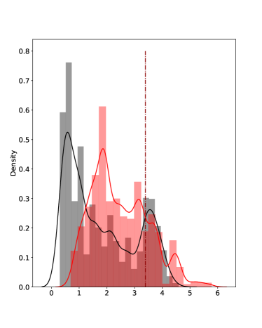
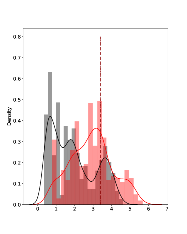
Figure 1: Empirical densities of anomaly scores given by the naive approach for uncontaminated time series in black and contaminated time series in red, on the train set (left) and on a test set (right). The dotted dark red line represents the cut-off value.

As shown in Figure 1, the naive approach results in a non-negligible overlapping region between the two densities, both on the train set (left) and for the test set (right). This region represents the anomaly score associated with time series that could be either contaminated or uncontaminated. The uncertainty regarding the nature of the observation when its anomaly score belongs to this region is relatively high in comparison with observations whose anomaly scores lie on the extreme left-hand or right-hand side of the calibrated cut-off value. Moreover, because we are not able to provide a clear separation between the scores of uncontaminated and contaminated time series, we may expect the model to mislabel future observations, resulting in a high rate of false positives and true negatives.

Neural network approach

In view of getting a clearer separation of the densities, we propose an alternative approach for the computation of the anomaly scores built upon the reconstruction errors. Let $F$ denote the function that associates with each reconstruction error $\varepsilon^{i}$ its anomaly score. In the naive approach, $F$ corresponds to the $\ell^{2}$-norm. Hereafter, $F$ instead represents the outputs of a feedforward Neural Network (NN). The training of the corresponding NN aims at minimizing a loss function that reflects our ambition to construct a function $F$ giving accurate anomaly scores. The network used for computing the anomaly scores is defined by

$$F(\varepsilon)=\left(h^{H}\circ h^{H-1}\circ\dots h^{2}\circ h^{1}\right)(\varepsilon),$$

where $h^{i}(\varepsilon)=\left(W^{i}\cdot\varepsilon+b^{i}\right)^{+}$ represents the computation carried in the $i$-th layer of the neural network with $n_{h}^{i}$ hidden units. $H$ stands for the number of layers of the NN, with ReLU activation applied element-wise. We finally estimate the labels from the outputs following $\bm{\hat{A}}=\mathds{1}_{\left\{(F(\bm{\varepsilon})-s)^{+}>0\right\}}$.

The idea of the learning is to calibrate the weights $\bm{W}:=\left\{W^{i}\in\mathbb{R}^{n_{h}^{i}\times n_{h}^{i-1}},i=2,\dots,H\right\}$ and the biases $\bm{b}:=\left\{b^{i}\in\mathbb{R}^{n_{h}^{i}},i=1,\dots,H\right\}$ such that the NN is able to accurately assess to which extent a time series is contaminated, with a clear distinction between the anomaly scores assigned to uncontaminated time series and those assigned to the contaminated ones, while integrating the calibration of the cut-off value $s$ as part of the learning. We denote by $\Theta:=\{\bm{W},\bm{b},s\}$ the set of parameters to be calibrated through the NN training. To meet these needs, the loss we minimize during the learning is given by

$$\mathcal{L}_{\Theta}\left(\bm{A},\hat{\bm{A}}\right)=\mathrm{BCE}(\bm{A},\bm{\hat{A}})+\mathrm{AUCDensity}^{u}_{\bm{A},F(\bm{\varepsilon})}+\mathrm{AUCDensity}^{c}_{\bm{A},F(\bm{\varepsilon})},$$ (5)

where

$$BCE(\bm{A},\bm{\hat{A}})=-\frac{1}{n}\sum_{i}\left(A^{i}\log(\hat{A}^{i})+(1-A^{i})\log(1-\hat{A}^{i})\right)\,$$

is the binary cross-entropy, a well-known loss function classically used for classification problems. To this first component of our loss function, we add two components that aim at downsizing the overlapping region between the density of anomaly score of both types of observations. In order to have a control on the latter, we consider $\mathrm{AUCDensity}^{u}$ and $\mathrm{AUCDentsity}^{c}$, which correspond to the area under the curve of the probability density function of anomaly scores the model assigns to contaminated and uncontaminated observations, respectively, i.e

$$\mathrm{AUCDensity}^{u}(s)=\int_{s}^{\infty}\hat{f}^{u}_{\bm{A},F(\bm{\varepsilon})}(\omega)d\omega\;,\quad\quad\quad \mathrm{AUCDensity}^{c}(s)=\int_{-\infty}^{s}\hat{f}^{c}_{\bm{A},F(\bm{\varepsilon})}(\omega)d\omega\,.$$ (6)

The bounds of these integrals depend on the cut-off value $s$ and define the region for which we want the probability density functions to be as small as possible, which allows us to estimate $\hat{s}$. The estimated probability density functions $\hat{f}^{u}_{A,F(\bm{\varepsilon})}$ and $\hat{f}^{c}_{A,F(\bm{\varepsilon})}$ depend on $F(\bm{\varepsilon})$, the scores assigned to contaminated time series identification model, and of the identification labels $\bm{A}$. We describe with Algorithm 2, the scoring and cut-off value calibration achieved by the calibration of a feedforward network with the loss (5). Each update of $\Theta$, AdamStep in Algorithm 2, is carried following the Adam optimization algorithm of (Kingma and Ba, 2014).

inputs : learning rate $lr$

number of maximum iterations $K$

kernel density estimator parameters $\mathcal{K}$,$\mathfrak{h}$

training data $\bm{\varepsilon}^{Train},\bm{A}^{Train}$

Initialize parameter $\Theta$, $\widehat{\mathcal{L}}=\infty$ and count index $k=0$;

while $k<K$ do

      

      $scores\leftarrow F_{\Theta}\left(\bm{\varepsilon}^{Train}\right)$ ;

       $scores^{c}\leftarrow scores\mathds{1}_{\bm{A}^{Train}=1}$;

       $scores^{u}\leftarrow scores\mathds{1}_{\bm{A}^{Train}=0}$;

       // Density estimation following (4) ;

      

       $\hat{f}^{u}_{\bm{A}^{Train},scores^{u}}=\mathrm{KernelDensityEstimator}(\mathcal{K},\mathfrak{h},scores^{u})$ ;

      

       $\hat{f}^{c}_{\bm{A}^{Train},scores^{c}}=\mathrm{KernelDensityEstimator}(\mathcal{K},\mathfrak{h},scores^{c})$

       // Loss evaluation following (5) and (6) ;

      

       $\mathrm{AUCDensity}^{u}\leftarrow\mathrm{NumericalIntegration}(\hat{f}^{u}_{\bm{A}^{Train},scores^{u}},s)$

       $\mathrm{AUCDensity}^{c}\leftarrow\mathrm{NumericalIntegration}(\hat{f}^{c}_{\bm{A}^{Train},scores^{c}},s)$

       $\bm{\hat{A}}\leftarrow\mathds{1}_{scores>s}$

       $\mathcal{L}\leftarrow\mathrm{BCE}\left(\bm{A}^{Train},\bm{\hat{A}}\right)+\mathrm{AUCDensity}^{u}+\mathrm{AUCDensity}^{c}$

       if  $\widehat{\mathcal{L}}>\mathcal{L}$  then

             $$

            ^L←L;

            

             $\widehat{\Theta}\leftarrow\Theta$;

            

       end if

      $$

      Θ←AdamStep(L,Θ,lr);

      

       $k\leftarrow k+1$;

      

end while

outputs : best calibrated parameter $\widehat{\Theta}=\{\widehat{\bm{W}},\hat{\bm{b}},\hat{s}\}$.

Algorithm 2 Scoring and cut-off calibration

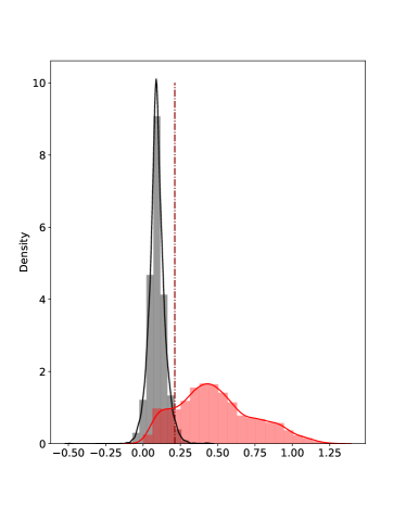
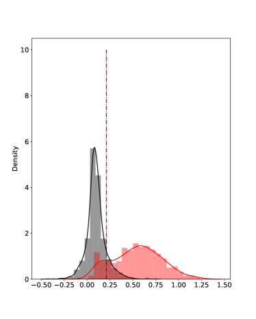
Figure 2: Empirical densities of anomaly scores given by the NN approach for uncontaminated time series in black and contaminated time series in red, on the train set (left) and on a test set (right). The dotted dark red line represents the calibrated cut-off value $\hat{s}$.

Approach $\mathrm{AUCDensity}^{u}$ $\mathrm{AUCDensity}^{c}$ Naive 0.1725 0.7898 NN 0.05153 0.1550 Approach $\mathrm{AUCDensity}^{u}$ $\mathrm{AUCDensity}^{c}$ Naive 0.1897 0.6354 NN 0.1290 0.1367

Table 1: AUC obtained with the naive and the NN approaches for the train set (left) and the test set (right).

Table 1 shows that with the NN approach the densities of scores assigned to each type of time series display the expected behaviours on the left-hand (right-hand) side of the cut-off value for contaminated (uncontaminated) time series, on both the train and test sets. Actually, the lower $\mathrm{AUCDensity}^{u}$ ($\mathrm{AUCDensity}^{c}$), the lower the number of uncontaminated (contaminated) time series to which are assigned anomaly scores above (below) the cut-off value, which prevents mislabelling.

Once the features $\bm{\varepsilon}$ and the calibrated NN are provided, the contaminated times series identification model is ready for use. This step is described by Algorithm 3.

inputs : time series to analyze $X^{i}$,

calibrated model parameter $\widehat{\Theta}$,

$\varepsilon^{i}\leftarrow\mathrm{PCAFeaturesExtraction}(X^{i})$;

;

  // cf. Algorithm 1 in Section 2.3

$score^{i}\leftarrow F_{\widehat{\Theta}}(\varepsilon^{i})$;

$\hat{A}^{i}\leftarrow\mathds{1}_{score^{i}>\hat{s}}$;

outputs : identification label $\hat{A}^{i}$.

Algorithm 3 Contaminated time series identification model

2.5 Anomaly Localization Step

Once the time series containing an anomaly have been identified, the second step of our approach aims at localizing an abnormal observation among each contaminated time series. Again we use the reconstruction errors defined in (3) as inputs of this second step. The difference lies on the transformation these reconstruction errors undergo before labelling the different time stamp observations. Namely, we now consider the following transformation of the reconstruction errors:

$$F(\varepsilon^{i})=\lvert\varepsilon^{i}\rvert=\lvert X^{i}-\widehat{X}^{i}\rvert,$$

with $\lvert\cdot\rvert$ meant component wise. The model input $F(\varepsilon^{i})\in\mathbb{R}^{p}_{+}$ is thus assigned to each time series $X^{i}\in\mathbb{R}^{p}$. The time stamp of occurrence of the anomaly is given by

$$\widehat{L}^{i}:=\arg\max_{j}\left\{F(\varepsilon^{i}_{t_{j}}):j\in\{1,\ldots,p\}\right\}.$$

Algorithm 4 recaps the anomaly localization model.

inputs : time series $X^{i}$ to analyze.

$\varepsilon^{i}\leftarrow\mathrm{PCAFeaturesExtraction}(X^{i})$

$\widehat{L}^{i}\leftarrow\arg\max_{\jmath}\left\{\lvert\varepsilon^{i}_{t_{\jmath}}\rvert:\jmath\in\{1,\ldots,p\}\right\}\;$

outputs : anomaly location $\widehat{L}^{i}$.

Algorithm 4 Anomaly Localization Model

Note that anomalies are not necessarily extrema. For this reason, the above PCA features extraction step is necessary. Building on the reconstruction errors, the model identifies these extrema-anomalies, but also abnormal observations which are not necessarily extrema. This subtlety of the nature of the observations underlines the importance of going further than taking the index of the highest observed value of the contaminated time series $X^{i}$.

Figure 3: Flow chart of our two step anomaly detection model (PCA NN), depicting the process a time series $X$ goes through.

The flow chart of Figure 3 along with Algorithm 5 summarize our approach. When a time series $X$ is given to our model, we suggest a new representation of $X$, namely $\varepsilon$, through a features engineering step involving PCA. The resulting representation $\varepsilon^{i}$ feeds the first component of the model, i.e. the identification step, which evaluates the time series propensity of being contaminated. The optimal parameter $\widehat{\Theta}$ of the identification model solves

$$\widehat{\Theta}=\arg\min_{\Theta=\left(\bm{W},\bm{b},s\right)}\sum_{X\in\bm{X}}\mathcal{L}_{\Theta}\left(A,\hat{A}\right),$$

where $\hat{A}=\mathds{1}_{F\left((\Omega\Omega^{\top}-I_{p})X\right)>s}$ and $\mathcal{L}_{\Theta}$ is the loss function defined in (5). Then, if the model considers the time series as contaminated, the localization model takes over to localize the abnormal value in $X$. For this second step of the model, the time stamp of occurrence of the anomaly is given by

$$\arg\max_{j}\quad\left\{\left(X\left(\Omega^{\top}\Omega-I_{p}\right)\right)_{j}:j\in\{1,\ldots,p\}\right\}$$

Finally, the anomaly is imputed. As our approach integrates the computation of a reconstruction of the time series, we could replace the anomaly with the corresponding reconstructed value. The model will be then able to detect the anomaly and suggest an imputation value. However, numerical tests described in Section 6.1 show that imputations with naive approaches perform better.

inputs : time series $X^{i}$ to analyze,

calibrated identification model parameter $\widehat{\Theta}$

$\widehat{A}^{i}\leftarrow\mathrm{IdentificationModel}(X^{i},\widehat{\Theta})$ // Algorithm 3

if $\widehat{A}^{i}=1$ then

       $\widehat{L}^{i}\leftarrow\mathrm{LocalizationModel}(X^{i})$ // Algorithm 4

end if

outputs : identification label $\widehat{A}^{i}$,

              anomaly localization $\widehat{L}^{i}$.

Algorithm 5 Anomaly Detection Model

3 Data Generation Process

Since anomalies are rare by definition, real data sets are very imbalanced: the proportion of anomalies compare to normal observations is very small, making the learning phase of the model difficult. This has led us to first consider synthetic data for the model calibration. The corresponding data set is obtained through a three-step process including time series simulations, contamination and data augmentation. We point out that, in the data simulation, care was taken to ensure that the generated data sets stay realistic. In particular, only few anomalies were added to time series as described in Section 3.2. To this extent, we still face the problem of scarcity of anomalies in this synthetic framework, and we provide some preprocessing steps to sidestep this issue as well.

3.1 Data Simulation

In this section, we describe the model used to simulate the data. Recall that our primary motivation is to detect anomalies in financial time series. For that purpose, we consider share price sample paths generated through the Black and Scholes model, i.e. geometric Brownian motions. Under this framework, the share price $S_{t}$ is defined by

$$S_{t}=S_{0}\exp\left(\left(\mu-\frac{1}{2}\sigma^{2}\right)t+\sigma W_{t}\right).$$ (7)

where $W$ represents a standard Brownian motion, $\mu$ the drift, $\sigma$ the volatility of the stock and $S_{0}$ the initial stock price.

Let $N$ stocks $S^{1},\ldots,S^{N}$ simulated simultaneously from this model, where $S^{i}:=\left\{S_{t_{0}}^{i},S_{t_{1}}^{i},\dots,S_{t_{T}}^{i}\right\}$ is the time series of length $T$ representing the (time discretized) path diffusion of the $i$-th stock. Each stock $S^{i}$ has its own drift $\mu^{i}$, volatility $\sigma^{i}$ and initial value $S^{i}_{t_{0}}$. The paths parameters are selected randomly according to

$$S_{t_{0}}^{i}\sim\mathcal{N}\left(100,1\right),\quad\quad\mu^{i}\sim\mathcal{U}\left([0.01,0.2]\right),\quad\quad\sigma^{i}\sim\mathcal{U}\left([0.01,0.1]\right),\quad\,i=1,\ldots,N.$$ (8)

For the sake of realism, the Brownian motions driving the $N$-stocks are correlated. The contamination of the obtained time series by anomalies is described in the next section.

3.2 Time Series Contamination

We apply a quite naive approach to introduce anomalies into our time series. We introduce the same fixed number of anomalies $n^{anom}$ to each time series by applying a shock on some original values of the observed time series. Formally, the $\jmath$-th added anomaly is characterized by its location $t_{\jmath}$ corresponding to the time stamp at which the anomaly has occurred, its shock $\delta_{\jmath}$, the amplitude of the shock is given by $|\delta_{\jmath}|$ and its sign by $\mathrm{sgn}\left(\delta_{\jmath}\right)$. We denote by $S^{a,i}$ the time series resulting from the contamination of the $i$-th clean time series $S^{i}$. For $i\in\{1,\dots,N\}$, let $\mathcal{J}^{i}$ be the set of indices of the time stamps at which an anomaly occurs for the $i$-th time series. For $\jmath\in\mathcal{J}^{i}$, the abnormal values are

$$S_{t_{\jmath}}^{a,i}=S_{t_{\jmath}}^{i}\left(1+\delta_{\jmath}\right).$$ (9)

The location, sign and amplitude of the shocks are generated randomly according to uniform distributions:

$$\mathcal{J}\sim\mathcal{U}_{N,n^{anom}}\left(\{1,\ldots,p\}\right),\quad\quad\mathrm{sign}\left(\delta\right)\sim\mathcal{U}_{N,n^{anom}}\left(\{-1,1\}\right),\quad\quad\lvert\delta\rvert\sim\mathcal{U}_{N,n^{anom}}\left([0,\rho]\right),$$

where $\rho$ is an upper bound on the shock amplitude.

We define the anomaly mask matrix $\mathbb{R}^{N\times T}$ by setting, for $i=1,\ldots,N$, and $j=1,\ldots,T$,

$$\mathcal{T}_{i,j}=\begin{cases}1+\delta_{j}&\text{if $j\in\mathcal{J}^{i}$.}\\ 1&\text{otherwise.}\end{cases}$$ (10)

Under this framework, when we incorporate the anomalies to the clean time series driven by the geometric Brownian motion, we assign labels to the time series observations according to whether the values correspond to anomalies or normal observations. We thus provide the labels $Y^{i}_{t_{j}}$ associated with each value $S_{t_{j}}^{a,i}$. Hence, for $i=1,\ldots,N$, and $j=1,\ldots,T$,

$$Y^{i}_{t_{j}}=\begin{cases}1&\text{if $j\in\mathcal{J}^{i}$.}\\ 0&\text{otherwise.}\end{cases}$$ (11)

Algorithm 6 recaps the time series contamination procedure, where AnomalyMask and GetLabels refer to the operators defined by (10) and (11).

inputs : amplitude range $\rho$,

number of anomalies to add in time series $n^{anom}$,

data $\bm{S}$

$\mathrm{sgn}\left(\delta\right)\leftarrow\mathcal{U}_{N,n^{anom}}\left(\{-1,1\}\right)$

$\lvert\delta\rvert\leftarrow\mathcal{U}_{N,n^{anom}}\left(\{0,\rho\}\right)$

$\mathcal{J}\leftarrow\mathcal{U}_{N,n^{anom}}\left(\{1,\ldots,p\}\right)$

$\mathbb{R}^{N\times T}\ni\mathcal{T}\leftarrow\mathrm{AnomalyMask}(\mathcal{J},\delta)$

$\bm{S}^{a}\leftarrow\bm{S}\circ\mathcal{T}$

$Y\leftarrow\mathrm{GetLabels}\left(\mathcal{J}\right)$

outputs : time series with anomalies $\bm{S}^{a}$,

              labels associated with each value of the time series $\bm{Y}$.

Algorithm 6 Data Contamination

3.3 Data Augmentation

By definition, anomalies are rare events and thus represent only a low fraction of the data set. Yet the suggested approach needs an important training set for an efficient learning. To overcome this issue, we apply a sliding window data augmentation technique (Le Guennec et al., 2016). This method not only extends the number of anomalies within the data set, but also allows the model to learn that anomalies could be located anywhere in the time series. It consists in extracting $N_{p}=T-p+1$ sub-time series of length $p$ of the initial observed time series of length $T$.

Note that we have to split the data into train and test sets before augmentation to guarantee that the time series considered in the training set do not share any observation with the ones we use for the model evaluation. In view of simplification, we introduce the data augmentation process, without loss of generality, for $\bm{S}$ and $\bm{Y}$. In practice this process has to be applied to $\bm{S^{Train}}$,$\bm{Y^{Train}}$ and $\bm{S^{Test}}$, $\bm{Y^{Test}}$ separately.

For $i=1,\ldots,N$ and $q\in\{1,\ldots,N_{p}\}$, the sub-time series $S^{i,q}$ and the associated labels $Y^{i,q}$ are defined by (see Algorithm 7)

$$S^{i,q} =\left\{S_{t_{j}}^{i}\,,\ j=q,\dots,q+p-1\right\}$$

$$Y^{i,q} =\left\{Y_{t_{j}}^{i}\,,\ j=q,\dots,q+p-1\right\}.$$

Each sub-time series $S^{i,q+1}$ thus results from the shift forward in time of one observation of the previous sub-time series $S^{i,q}$. The final data set $\bm{X}$ and the labels $\bm{{}^{s}Y}$ are then defined as the matrices whose rows correspond to the sub-time series $S^{i,q}_{q=1,\ldots,N_{p};i=1,\ldots,N}$, and $Y^{i,q}_{q=1,\ldots,N_{p};i=1,\ldots,N}$, respectively, i.e.

$$\bm{X} =\left(S^{1,1},S^{1,2},\ldots,S^{1,N_{p}},S^{2,1},\ldots,S^{i,q},\ldots,S^{N,N_{p}}\right)^{\top},$$

$$\bm{{}^{s}Y} =\left(Y^{1,1},Y^{1,2},\ldots,Y^{1,N_{p}},Y^{2,1},\ldots,Y^{i,q},\ldots,Y^{N,N_{p}}\right)^{\top}.$$

With this data configuration, an observation refers to a time series $S^{i,q}$ obtained through the sliding window technique. Two observations may represent the same stock but on different time intervals.

inputs : window size $p$,

              data and labels $\bm{S}$,$\bm{Y}$;

Initialize empty slided time series and labels matrices $\bm{X}$, $\bm{{}^{s}Y}$;

for i :=1 to N do

       for q :=1 to $N_{p}$ do

             $S^{i,q}\leftarrow\left\{S_{t_{j}}^{i}|j\in\{q,\dots,q+p-1\}\right\}$

            

            $Y^{i,q}\leftarrow\left\{Y_{t_{j}}^{i}|j\in\{q,\dots,q+p-1\}\right\}$

            

       end for

      $\bm{X}\leftarrow\mathrm{Concatenate}\left(\bm{X},S^{i,q}\right)$

      $\bm{{}^{s}Y}\leftarrow\mathrm{Concatenate}\left(\bm{{}^{s}Y},Y^{i,q}\right)$

      

end for

outputs : resulting slided time series and labels $\bm{X},\bm{{}^{s}Y}$

Algorithm 7 Data Augmentation with sliding window technique

While the fact that the observations share the same values may be argued to wrongly impact the learning process, we point out that a real benefit can be drawn from this situation. Indeed, thanks to this sliding window technique, the number of anomalies is considerably increased. This technique also allows the model to learn that anomalies could be located anywhere in the time series, reducing the dependency on the event location (Um et al., 2017).

However, once we apply the sliding window technique, we do not only extend the number of contaminated time series: the number of uncontaminated time series is also increased. But the minority class (contaminated time series) has, at least, a significant number of instances, denoted by $N^{c}$. In order to get a more balanced data set for the training set, we perform an undersampling, selecting randomly $N^{c}$ observations from the $N^{u}$ uncontaminated time series without any anomalies (RandomSampling in Algorithm 8). The resulting retained number of observations $2N^{c}$ is now sufficient to train the model. The test set in turn is imbalanced. To sharpen the imbalanced characteristic of the test set, we specify a contamination rate $r_{c}$, which corresponds to the rate of contaminated time series in the data set. The construction of the test set is described in Algorithm 8.

Inputs : slided data and labels $\bm{X}$,$\bm{{}^{s}Y}$,

              contamination rate $r_{c}$ (for test set)

$\bm{X},\bm{{}^{s}Y}\leftarrow\bm{X}\mathds{1}_{\mathrm{sum}(\bm{{}^{s}Y})\leq 1},\bm{{}^{s}Y}\mathds{1}_{\mathrm{sum}(\bm{{}^{s}Y})\leq 1}$ ;

  // Keep time series with at most one anomaly.

if Train set then

      

      $N^{c}=\mathrm{Card}\left(\bm{{}^{s}Y}\mathds{1}_{\mathrm{sum}(\bm{{}^{s}Y})=1}\right)$

       // Randomly select the indexes of $N^{c}$ uncontaminated time series ;

      

       $\mathrm{index}^{u}=\mathrm{RandomSampling}\left(\left\{i;\;\mathrm{sum}(Y_{s}^{i})=0,i\in\{1,\ldots,NN_{p}\}\right\},N^{c}\right)$

end if

if Test set then

      

      $N^{c}=\mathrm{Card}\left(\bm{{}^{s}Y}\mathds{1}_{\mathrm{sum}(\bm{{}^{s}Y})=1}\right)$

       ;

       $N^{u}=\left\lceil\frac{N^{c}(1-r_{c})}{r_{c}}\right\rceil$

       // Randomly select the indexes of $N^{c}$ uncontaminated time series ;

      

       $\mathrm{index}^{u}=\mathrm{RandomSampling}\left(\left\{i;\;\mathrm{sum}(Y_{s}^{i})=0,i\in\{1,\ldots,NN_{p}\}\right\},N^{u}\right)$

      

end if

$\mathrm{index}^{c}=\left\{i;\;\mathrm{sum}(Y_{s}^{i})=1,i\in\{1,\ldots,NN_{p}\}\right\}$

$\bm{X}\leftarrow\left(X^{i},\mathrm{for}\;i\;\in\;\mathrm{index}^{u}\cup\mathrm{index}^{c}\right)$

$\bm{{}^{s}Y}\leftarrow\left(Y_{s}^{i},\mathrm{for}\;i\;\in\;\mathrm{index}^{u}\cup\mathrm{index}^{c}\right)$

outputs : time series $\bm{X}$ with at most one anomaly,

corresponding labels for identification task $\bm{A}$,

corresponding labels for localization task $\bm{L}$.

Algorithm 8 Time series selection

As mentioned in Section 2.2, Algorithm 5 is designed to predict the localization of only one anomaly, (if there is more than one anomaly in the time series, it should be run iteratively as detailed in Section 2.2). Here we only consider time series with at most one anomaly (without loss of generality).

Assumption 1

A time series $S^{i,q}$ contains at most one anomaly among all its observed values.

We assign the identification label $A^{i,q}$ (see Section 2.1) to each $S^{i,q}$ following the rule

$$A^{i,q}=\sum_{j=q}^{q+p-1}Y^{i}_{t_{j}}=\begin{cases}1&\text{if there is an anomaly among the observed values of $S^{i,q}$}\\ 0&\text{otherwise.}\end{cases}$$

Regarding the localization labels, we recall that they only concern the time series with an anomaly, therefore $L^{i,q}$ is defined following

$$L^{i,q}=\arg\max_{j}Y^{i,q}=\arg\max_{j}\left\{Y_{t_{j}}^{i}\,,\ j=q,\dots,q+p-1\right\}$$ (12)

With Algorithm 9, we give a rundown of the construction process of the identification and localization labels, namely $\bm{A}$ and $\bm{L}$ departing from $\bm{{}^{s}Y}$.

The supervised learning framework is adopted herein, since we have at our disposal labelled data.

The resulting matrices with the observed values of the time series in $\bm{X}$ the associated identification labels in $\bm{A}$ and localization labels in $\bm{L}$ constitute the data set used for our model calibration and evaluation.

Inputs : slided labels $\bm{{}^{s}Y}$;

$\bm{A}\leftarrow\mathrm{sum}(\bm{{}^{s}Y})$ ;

$\bm{L}\leftarrow\arg\max\left\{\bm{{}^{s}Y}\mathds{1}_{\mathrm{sum}(\bm{{}^{s}Y})=1}\right\}$

outputs : corresponding labels for identification task $\bm{A}$,

corresponding labels for localization task $\bm{L}$.

Algorithm 9 Time series labelling

4 Model Evaluation: Setting the Stage

After introducing the relevant performance metrics used to assess the PCA NN performance, we describe the synthetic data used for the numerical experiments of Sections 5 to 7. We then briefly describe the process of the latent space dimension calibration.

4.1 Performance Metrics

Common methods to assess the performance of binary classifiers include true positive and true negative rates, as well as ROC (Receiver Operating Characteristics) curves, displaying the true positive rate against the false positive rate. These methods, however, are uninformative when the classes are severely imbalanced. In this context, $F_{1}$-score and Precision-Recall curves (PRC) should be used (Brownlee, 2020; Saito and Rehmsmeier, 2015). They are both based on the values of

$$\mathrm{Precision}(s)=\frac{\text{true positives}}{\text{true positives}+\text{false positives}}$$

against the values of

$$\mathrm{Recall}(s)=\frac{\text{true positives}}{\text{true positives}+\text{false negatives}}\,$$

where $s$ is a cut-off probability varying between $0$ and $1$. Precision quantifies the number of correct positive predictions out all positive predictions made, while Recall (often also called Sensitivity) quantifies the number of correct positive predictions out of all positive predictions that could have been made. Both focus on the Positives class (the minority class, anomalies) and disregard the Negatives (the majority class, normal observations).

Our $F_{1}$-score (Chinchor and Sundheim, 1993; Van Rijsbergen, 1979) combines these two measures in a single index defined as

$$F_{1}=2\cdot\frac{\mathrm{Precision}\cdot\mathrm{Recall}}{\mathrm{Precision}+\mathrm{Recall}}.$$ (13)

The closer the $F_{1}$-score to 1, the better the prediction model.

A PRC displays the values of Precision and Recall as the cut-off $s$ varies from $0$ to $1$. The PRC of a skillful model bows towards the point with coordinates $(1,1)$. The curve of a no-skill classifier is an horizontal line at some $y$-level proportional to the proportion of Positives in the data set. For a balanced data set this proportion is just 0.5 (Brownlee, 2020).

PRC and $F_{1}$-score are complementary in our approach. The $F_{1}$-score is used on the anomaly scores outcomes of the models, to identify the best configuration and the best model. A PRC is used to select the best cut-off value used in the prediction of the two classes, for each model.

4.2 Synthetic Data Set

The anomaly detection task is performed on $N=20$ stocks simultaneously. The stock prices are diffused according to the Black and Scholes model. Each stock has its own drift and volatility and the $20$ stocks are correlated, as described in Section 3. Each time series represents $T=1,500$ daily stock prices, split into two sets. The first $1,000$ observations, corresponding to the train set, are used to learn the model parameters, i.e. the PCA transfer matrix and the NN weights and biases. The last $500$ observations, corresponding to the test set, are used to assess the quality of the estimated parameters when applied to unseen samples. For the application of the sliding window technique, we set the length of the resulting time series $p$ to be 206. Table 2 sums up the composition of each data set before and after data augmentation.

Nb of Time Series Nb of Observed values per time series Nb of anomalies Train set 20 1,000 $4\times 20$ Test set 20 500 $2\times 20$

Nb of Time Series Nb of Observed values per time series Nb of anomalies Train set 12,000 206 6,000 Test set 2,500 206 400

Table 2: Data set composition (top) before and (bottom) after data augmentation.

We recall that both steps of the approach are preceeded by a features extraction step, for which the latent space dimension $k$ needs to be calibrated. As shown by the numerical results provided in Section C, the features extraction also guarantees the stationarity of the time series used for the anomaly detection task, $\bm{\varepsilon}$.

4.3 Calibration of the Latent Space Dimension

When performing PCA, $k$ is determined through a scree-plot, which is the representation of the proportion of variance explained by each component. The optimal $k$ corresponds to the number of principal components explaining a given level of the variance of the original data. However, this method has its limitation as stated in (Linting et al., 2007). More importantly, it is not suitable for our approach. Indeed, in our case, the number of selected principal components must achieve a trade-off between information and noise in the latent space. If we consider a too low number of principal components, we may lose information regarding the normal observations, leading to false alarms. If a too high number of principal components is retained, we may include components representing noise, which prevents the model from detecting some anomalies.

To select the optimal dimension of the latent space, we consider the distribution of anomaly scores obtained through the naive approach of Section 2.4, empirically calibrating a cut-off $\hat{s}$ through the non parametric estimation of the distribution of the anomaly scores of uncontaminated and contaminated time series. We chose to calibrate the dimension of the latent space with the naive approach, because using the NN to this end would be very costly. Hence, for each $k=5,10,\dots,200$, we construct a PCA model from which we infer reconstruction errors which are then converted into anomaly scores. Based on these anomaly scores, we tune the cut-off value $\hat{s}$ thanks to the distributions and we finally convert the scores into labels. We evaluate the predictions of the naive approach for each value of $k$. The results on the evaluation metrics on the train set, as legitimate to choose $k$, are represented on Figure 4. The highest values are reached for $k\in\{40,\dots,145\}$. The performance seems to be stable in terms of $F_{1}$-score and accuracy. Therefore, for computational reasons, we choose the optimal $k$ to be 40.

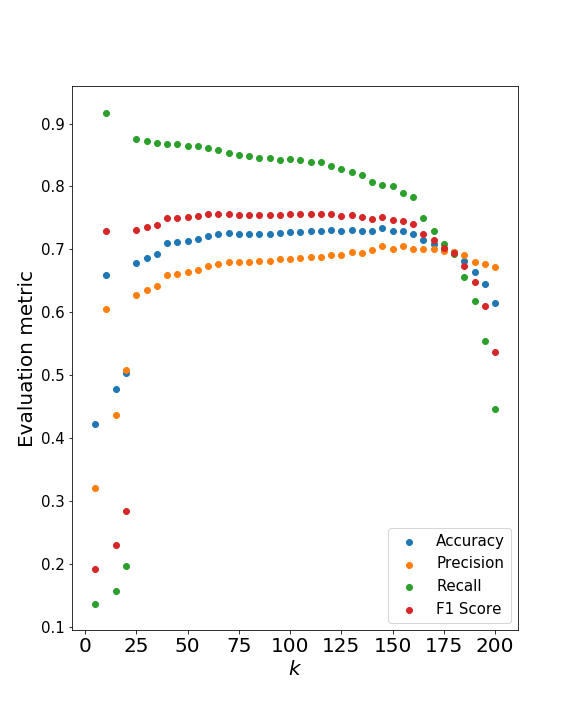
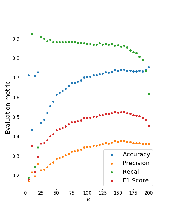
Figure 4: Performance metrics on train (left) and test (right) sets with respect to the number of principal component $k$.

Figure 4 also shows, as expected, a downward trend of the scores when represented against the highest values of $k$. This demonstrates that when a high level of variance is explained, it become much harder to perform anomaly detection based on the reconstruction errors.

5 Model Evaluation: Main Results

We evaluate the performance of the identification and localization stages of our approach on synthetic data, using appropriate performance metrics. We demonstrate numerically the efficiency of the PCA NN over baseline anomaly detection algorithms.

5.1 Contaminated Time Series Identification Step

For the features extraction step, we considered a latent space dimension $k=40$. The NN built to compute the anomaly scores and convert them into labels was calibrated on the train set. The result of this calibration is shown in Table 3.

Data set	Accuracy	Precision	Recall	$F_{1}$-score
Train set	90.97 %	97.36%	84.21%	90.31 %
Test set	88.58%	61.26%	85.27%	71.30%

Table 3: Performance evaluation of suggested model on synthetic data set for identification step.

Figure 5 shows two contaminated time series identified as such by the model. Figure 6 displays two examples of time series without anomalies accurately identified by the model. Figure 7 displays two time series misidentified by the model.

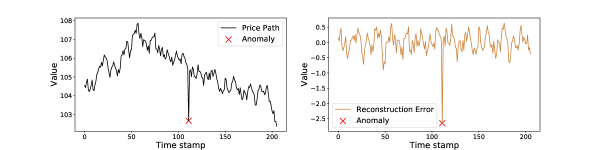
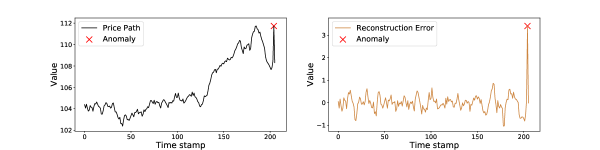
Figure 5: Two examples of contaminated time series accurately identified by the model. The stock path and the reconstruction errors are represented in black and brown. The red cross shows the anomaly localization.

When an observation deviates significantly from the rest of the time series values, the model is able to recognise that the concerned time series contains an abnormal observation.

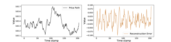
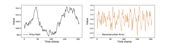
Figure 6: Two examples of uncontaminated time series accurately identified by the model. The stock path and the reconstruction errors are represented in black and brown.

In Figure 6 with uncontaminated time series, we see that even when there is a local upward trend in the time series values, the model is able to make the distinction between this market move and the occurrence of an anomaly.

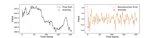
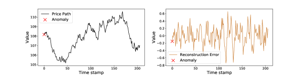
Figure 7: Two examples of time series misidentified by the model. The stock path and the reconstruction errors are represented in black and brown. The red cross shows the anomaly localization.

The last set of time series displays some limits of the model. The top graphs in Figure 7 represent the situation where the model did not manage to identify the contaminated time series. One explanation could be that the size of the anomaly is not significantly large enough to be spotted by the model. Indeed, looking at the graph, the time series does not seem to contain any anomaly. In contrast, the bottom graphs in Figure 7 show a stock price path predicted to be contaminated whereas it is not.

We illustrate the robustness of the approach by assessing the model predictions on $100$ distinct data sets. Table 4 shows the mean and standard deviation over the multiple runs.

Data set	Accuracy	Precision	Recall	$F_{1}$-score
Train set	79.02% (2.4%)	78.69% (2.7%)	79.74% (4.6%)	79.13% (2.7%)
Test set	77.79% (3.9%)	41.87% (5.2%)	80.16% (6.4%)	54.82% (5.2%)

Table 4: Mean (standard deviation) of performance metrics of the suggested model over multiple runs for the identification step.

5.2 Anomaly Localization Step

Regarding the localization step, the dummy approach consists in taking the argmax of time series observations as the anomaly location. We distinguish between two cases, anomalies which are extrema and anomalies which are not. The quality of the detection of our model is assessed for both types of anomalies. The results are displayed in Tables 5 and 6.

Data set	Accuracy	Precision	Recall	$F_{1}$-score
Train set	89.65% (34.87%)	89.81% (40.53%)	89.65% (34.88%)	89.68% ( 36.56%)
Test set	94.39% (27.78%)	94.49% (31.52%)	94.39% (27.78%)	94.38% (28.94%)

Table 5: Performance evaluation of the suggested model and (the dummy approach) on synthetic data set for the localization step on all type of anomalies.

Data set	Accuracy	Precision	Recall	$F_{1}$-score
Train set	84.22% (0%)	84.55% (0%)	84.28% (0%)	89.68% (0%)
Test set	91.92% (0%)	92.10% (0%)	91.92% (0%)	91.90% (0%)

Table 6: Performance evaluation of the suggested model and the dummy approach on synthetic data set for the localization step on non extrema anomalies.

Numerical tests show the necessity of the features extraction step for the anomaly localization task, as applying the dummy approach alone is not enough when the anomaly is not an extreme value. Figure 8 represents a stock price time series with the true and predicted anomaly location. In these examples, the locations are accurately predicted.

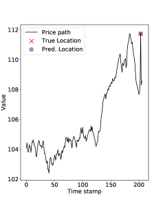
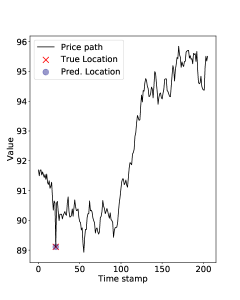
Figure 8: Anomaly localization prediction on two distinct time series.

To guarantee the robustness of the model on the anomaly location, we evaluate the model prediction on $100$ data sets. Table 7 shows the mean and standard deviation for the localization step of all types of anomaly.

Data set	Accuracy	Precision	Recall	$F_{1}$-score
Train set	89.58% (4.3%)	89.58% (4.3%)	89.96% (4.1%)	89.67% (4.3%)
Test set	89.49% (4.8%)	89.49% (4.8%)	90.00% (4.5%)	89.58% (4.7%)

Table 7: Mean (standard deviation) of performance metrics of suggested model over multiple runs for localization step on all type of anomalies.

Table 8 displays the results on the localization of non extrema anomalies. These results show the importance of the features extraction step. If we only consider the maximal observed value of the time series to be the anomaly, we would not be able to localize any non-extrema anomaly. Applying Algorithm 4 instead leads to satisfying anomaly detection rates.

Data set	Accuracy	Precision	Recall	$F_{1}$-score
Train set	85.23% (6.0%)	85.23% (6.0%)	85.87% (5.7%)	85.36% (6.0%)
Test set	85.17% (7.1%)	85.17% (7.1%)	86.04% (6.8%)	85.30% (7.1%)

Table 8: Mean (standard deviation) of performance metrics of suggested model over multiple runs for localization step on non-extreme anomalies.

5.3 Numerical Results Against Benchmark Models

To assess the performance, the suggested approach is compared numerically with well-known machine learning algorithms for anomaly detection, that is isolation forest (IF), local outlier factor (LOF), density based clustering of applications with noise (DBSCAN), k-nearest neighbors (KNN), and support vector machine (SVM), all reviewed in Section B. In addition to these state of the art techniques, we consider the recent anomaly detection technique proposed by Akyildirim et al. (2022), referred to as sig-IF, combining a features extraction step through path signatures computation with IF.

Tables 9 and 11 summarize the performance on the train and test sets of Section 3 of each model, for both the contaminated time series identification and the anomaly localization steps.

	Train		Test
Model	Accuracy	$F_{1}$-score	Accuracy	$F_{1}$-score
IF	42.31%	42.31%	69.64%	7.022%
LOF	59.95%	59.95%	90.00%	62.41%
DBSCAN	50.00%	66.67%	16.65%	28.53%
sig-IF	49.48%	49.23%	72.32%	15.19%
KNN	94.68%	94.39%	64.82%	26.69%
SVM	81.96%	82.33%	44.39%	27.44%
PCA NN	90.97%	90.31%	88.58%	71.30%

Table 9: Performance evaluation of unsupervised (upper part) and supervised (lower part) models for contaminated time series identification step.

Algorithm	IF	LOF	DBSCAN	KNN	SVM	sig-IF	PCA NN
Exec. Time	0.6915	0.2015	0.1275	1.725	4.572	2.776	0.003523

Table 10: Execution time in seconds for identification of contaminated time series step.

The following paragraphs provide similar conclusions drawn from the results on the identification and localization steps (see Tables 9 and 11).

For the unsupervised learning methods, since there is not a proper learning step, even though Tables 9 and 11 show the scores on the train and test set, these scores should be seen as the ones obtained by testing the models on independent data sets. For IF, LOF and DBSCAN models, the performance across the sets is not stable, as a significant difference could be observed between the scores on the train and test sets. The poor performance of unsupervised learning algorithms could be explained by the difficulty to estimate the contamination rate for IF and the LOF algorithms. For DBSCAN the poor performance is rather due to the high dimensionality of the data. As for the sig-IF approach, its performance in this specific case is not as overwhelming as when used to detect pump and dump operations in (Akyildirim et al., 2022). This difference in performance is driven by the fact that, in our case, signatures are computed on the stock price path only, since no additional information is available to describe the price path we are analyzing. For pump/dump detection, instead, signatures are computed on a set of variables path including the price path and additional variables paths helpful in the identification of the pumps/dumps attempts.

Regarding the supervised approaches, although KNN is outperforming the suggested approach on the training set, there is a non-negligible decrease of these scores on the test set. This may suggest an over-fitting on the training data, which makes KNN unable to generalize what it has learnt to unseen samples. The same trend is seen on the scores with our approach, however the loss is no as harsh as in the KNN case.

Hence, according to the results, our PCA based approach seems to be the most suitable method for the problem at stake of anomaly detection on time series. Its satisfying performance in terms of accuracy and $F_{1}$-score, as well as its low computational cost for both steps (see Tables 10 and 12), make the approach stand out.

	Train		Test
Model	Accuracy	$F_{1}$-score	Accuracy	$F_{1}$-score
IF	89.79%	2.296%	70.94%	1.611%
LOF	99.51%	0%	2.066%	0.9816%
DBSCAN	N/A	NA	NA	NA
sig-IF	N/A	N/A	N/A	N/A
KNN	99.99%	99.99%	95.56%	2.794%
SVM	NA	NA	NA	NA
PCA NN	89.65%	89.68%	94.39%	94.38%

Table 11: Performance evaluation of unsupervised (upper part) and supervised (lower part) models for anomaly localization step. Results for DBSCAN, sig-IF and SVM are not provided due to high computational cost.

Algorithm	IF	LOF	DBSCAN	KNN	SVM	sig-IF	PCA NN
Exec. Time	14.50	2.287	N/A	14.19	N/A	N/A	0.002004

Table 12: Execution time in seconds for the anomaly localization step. Results for DBSCAN, sig-IF and SVM are not provided due to high computational cost.

6 Model Evaluation: Additional Results

To take our approach a leap beyond classical anomaly detection algorithms, we evaluate the anomalies imputation suggested by the PCA NN approach. We also test the robustness of the calibrated cut-off value and examine the sensitivity of the PCA NN performance to the amplitude of the anomaly.

6.1 Anomalies Imputation

To assess the imputation values suggested by our approach, we start from time series simulated without anomalies, then we randomly select a time stamp of the time series and add a noise to the corresponding value following the methodology described in Section 3.

The imputation value the PCA NN suggests, is the reconstructed observation. This imputation technique is compared to naive methods of missing values imputation, namely backward fill (BF), consisting in replacing the anomaly by the previous value, and linear interpolation (LI). The choice of these imputation methods is motivated by their low computational cost. In fact, the PCA NN imputation comes at no additional cost as stated before. Therefore, we only challenge its performance using methods with similar complexity. To assess the quality of the imputation value suggested by each approach, we consider the following metrics. The imputation errors are computed on each time series $i$ as

$$\mathrm{ImputationError}^{i}=\sqrt{\sum_{j}\frac{\left(S^{i}_{t_{j}}-\widetilde{S}^{i}_{t_{j}}\right)^{2}}{n^{anom}}}\;,$$

where $\widetilde{S}^{i}$ refers to as the $i$-th path price with imputed values. The error on the covariance matrix is computed as

$$\mathrm{ErrCov}=\|\Sigma-\widetilde{\Sigma}\|_{\mathrm{Frob}},$$

where $\|\cdot\|_{\mathrm{Frob}}$ is the Frobenius norm, $\Sigma$ the sample covariance matrix, and $\widetilde{\Sigma}$ the covariance matrix estimated on the data after the anomalies have been replaced by their respective imputation values.

Each stock path was diffused and contaminated 100 times. The anomalies were then imputed following two baseline approaches (BF and LI). Figure 9 clearly shows that imputation using the reconstructed values with PCA reduces the imputation error but not as much as basic imputation techniques (LI and BF) as it is shown on Figure 10. Table 13 shows that the baseline imputation approaches achieve even lower errors on the estimation of the covariance matrix. Figure 11 shows a higher mean but a lower variance of the errors for the PCA-based imputation approach. In conclusion, it would be rather recommended to replace the flagged anomalies with approaches such as backward fill or linear interpolation.

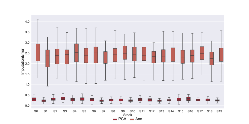
Figure 9: Boxplot representation of the distribution of the errors on time series imputation before the imputation of anomalies (Ano) and after replacing the anomalies with the reconstructed values suggested by PCA NN (PCA).

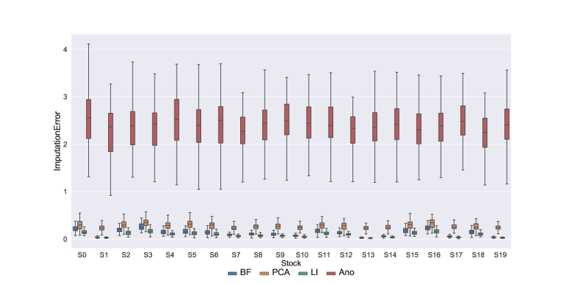
Figure 10: Boxplot representation of the distribution of the errors on time series imputation before the imputation of anomalies (Ano) and after replacing the anomalies; with the reconstructed values suggested by PCA (PCA), using linear interpolation (LI) and using backward fill (BF).

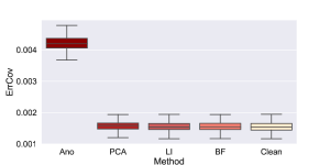
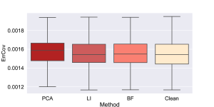
Figure 11: Boxplot representation of the distribution of the errors on covariance matrix (on several stocks paths samples). Ano, PCA NN, LI, BF and Clean refer to the errors on the covariance when estimated on time series with anomalies, time series after anomalies imputation following three approaches: imputation by the reconstructed values suggested by PCA (PCA), using linear interpolation (LI), with backward fill (BF) and time series without anomalies (Clean). The Ano, PCA NN, LI, BF and Clean errors on the covariance estimation are all represented (left). For better visualization we remove the Ano errors (right).

Method	Ano	PCA	LI	BF	Clean
Mean	0.004208	0.001575	0.001554	0.001554	0.001552
Standard deviation	0.000272	0.000165	0.000170	0.000172	0.000173

Table 13: Mean and standard deviation error on covariance matrix after imputation of anomalies with baseline methods.

A natural explanation to the relative inefficiency of the reconstruction value as imputation value comes from the fact that, by construction, the reconstructed value integrates in its computation the abnormal value, which is not the case when using other imputation techniques. Therefore, even if the reconstructed value is closer to the true value than it is to the abnormal value, the spread between the imputation and the true value is still significant. Figures 12 and 13 illustrate the latter with a plot of a reconstructed and original price path.

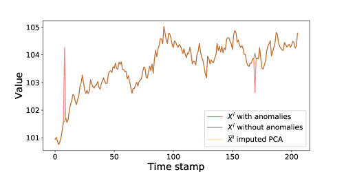
Figure 12: Original, contaminated and reconstructed stock price path.

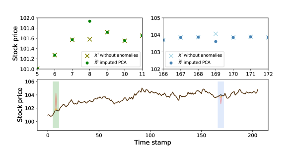
Figure 13: Original, contaminated and imputed stock prices path in black, red and orange. The two additional graphs represent the region around anomalies, where the cross and circle respectively show the true value of the stock and its value after imputation of the anomalies using the reconstructed value suggested by the PCA NN approach.

6.2 Cut-off Value Robustness

In most anomaly detection models, the cut-off value is a hand-set parameter. In our approach, the cut-off value is a model parameter and as such it is calibrated through the learning. Testing the robustness of the cut-off given by the model is therefore a must. The identification step is the unique step of the approach being concerned by the robustness, since it is the only step involving the cut-off calibration. Robustness is checked by shocking the suggested cut-off with different level of noise and observing the impact of these shocks on the model performance. We consider several shock amplitude $\gamma\in\pm\{10^{-4},10^{-3},10^{-2},10^{-1},1,2\}$. Table 14 reports the mean and standard deviation of the scores of the model. The cut-off calibrated on the synthetic training data sample is shocked. Scores on both train and test sets are computed using the shocked cut-off values.

$\gamma$ Accuracy Precision Recall $F_{1}$ $10^{-4}$ 0.9097 0.9736 0.8421 0.9031 -$10^{-4}$ 0.9097 0.9736 0.8421 0.9031 $10^{-3}$ 0.9097 0.9738 0.8419 0.9031 -$10^{-3}$ 0.9098 0.9737 0.8424 0.9033 $10^{-2}$ 0.9092 0.9747 0.8403 0.9025 -$10^{-2}$ 0.9098 0.9720 0.8439 0.9035 $10^{-1}$ 0.9042 0.9860 0.8201 0.8954 -$10^{-1}$ 0.9103 0.9563 0.8599 0.9056 0 0.9097 0.9736 0.8421 0.9031 1 0.7771 0.9994 0.5546 0.7133 -1 0.5183 0.5093 0.9998 0.6749 2 0.6284 1.0000 0.2567 0.4086 -2 0.5001 0.5000 1.0000 0.6667 $\gamma$ Accuracy Precision Recall $F_{1}$ $10^{-4}$ 0.8858 0.6126 0.8527 0.7130 $-10^{-4}$ 0.8858 0.6126 0.8527 0.7130 $10^{-3}$ 0.8858 0.6126 0.8527 0.7130 $-10^{-3}$ 0.8850 0.6105 0.8527 0.7116 $10^{-2}$ 0.8877 0.6179 0.8527 0.7166 $-10^{-2}$ 0.8838 0.6074 0.8527 0.7095 $10^{-1}$ 0.8984 0.6502 0.8432 0.7342 $-10^{-1}$ 0.8672 0.5653 0.8741 0.6866 0 0.8858 0.6126 0.8527 0.7130 1 0.9391 0.9435 0.6746 0.7867 -1 0.2660 0.1848 1.0000 0.3120 2 0.8949 0.9814 0.3753 0.5430 -2 0.1700 0.1670 1.0000 0.2862

Table 14: Performance evaluation after shocking the calibrated cut-off value for the training set (left) and for the test set (right).

Excluding the extreme cases where the shock amplitude is $\pm\{1,2\}$, one could see that the accuracy is barely impacted by the shocked cut-off values, both on the train and test sets. The interpretation of the remaining results is split in two and is applicable for both the training and test sets.

When negative shocks are applied, the model predicts more anomalies and less normal observations (compared to the predicted numbers with the calibrated cut-off value). Therefore, the model is able to identify anomalies which were missed initially. Hence, applying negative shocks increases the recall. As for the precision, i.e. the rate of correctly identified contaminated time series, since on left hand side of the cut-off value we are in the density region where contaminated time series represent the dominant class, the new position of the cut-off value leads to a misidentification of this type of observations. This entails a deterioration of the precision. Opposite behaviours of the precision and recall are observed when positive shocks are applied, since some abnormal time series are missed by the model.

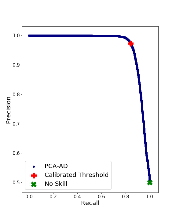
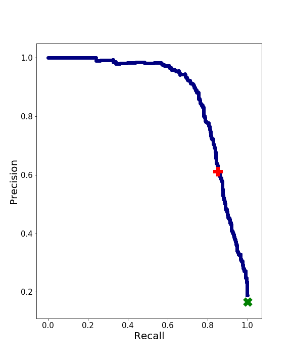
Figure 14: Precision-recall curve of the suggested model (in blue), scores with the calibrated threshold (red plus), no-skill model scores (green cross) for the training set (left) and a test set (right).

Figure 14 shows the precision and recall when cut-off values other than the one we calibrated are used in our model, on the train and test sets. These scores are also compared with the performance of the no-skill model. We note that our approach edges out the no-skill model on both sets. The area under the curve (AUC) score on the train set and the test set are respectively 0.97 and 0.87. This shows that we are better performing on the train set, which was expected, but the performance on test set is just as satisfying. These results reinforce our conclusions regarding the robustness of our approach. One can see that the calibrated cut-off value represents, for the train set, the point where an equilibrium is being reached between precision and recall. The calibrated cut-off allows to achieve high precision and recall scores, simultaneously. We conclude that the cut-off given by the model is suitable for the training samples and for unseen samples as well.

To briefly sum up this section, although we mentioned that some shocks on the cut-off value induce higher scores, the improvement over the scores with the calibrated cut-off value is not significant (unless high amplitude shocks are considered). The numerical tests and the precision-recall curves are consistent with the robustness of the cut-off value suggested by the approach.

6.3 Sensitivity to Anomaly Amplitude

Time series are manually contaminated as described in Section 3.2. The abnormal value $S^{a,i}_{t_{\jmath}}$ of the $i$-th time series results from a shock of the initial value of the time series denoted by $S^{i}_{t_{\jmath}}$ as stated in (9). We recall that the shock is represented by $\delta$, whereas its amplitude $\lvert\delta\rvert$ is uniformly drawn from $[0,\rho]$. Hence, $\rho$ is the parameter that ultimately controls the amplitude of the anomaly. Since $\rho$ is fixed by the user, it is interesting to investigate the sensitivity of the PCA NN approach performance to the amplitude of the shock.

The PCA NN approach evaluated in Sections 5.1-5.2 is calibrated on time series which were contaminated with shock amplitude drawn from $\mathcal{U}\left([0,\rho]\right)$ with $\rho=0.04$. For the data sets on which the model was calibrated and then evaluated, the anomalies were grouped according to the shock amplitude they result from. For the identification step, we distinguish four groups of contaminated times. For instance, the first line of Table 15 defines the first group of contaminated time series, for which the anomalies results from shock amplitude $\in{[}0.3091e-2,1.46e-2{[}$. For this first group with this specific range of amplitude, $77\%$ of the contaminated time series were identified during the PCA NN identification step.

Amplitude Range ($10^{-2}$)	Detection ratio
[0.309, 1.46[	0.77
[1.46, 2.34[	0.91
[2.34, 2.92[	0.96
[2.92, 3.78]	0.98

Table 15: Detection ratio of correctly identified contaminated time series on test set, with time series being grouped according to their anomalies shock amplitude.

Similarly, for the localization step, we consider four groups of anomalies. The first line of Table 16 represents the anomalies with shock amplitude $\in{[}0.309e-2,1.31e-2{[}$. $86\%$ of the anomalies belonging to this first group were correctly localized by the PCA NN localization step.

Amplitude Range ($10^{-2}$)	Detection ratio
[0.309, 1.31[	0.86
[1.31, 2.29[	1.00
[2.29, 2.88[	1.00
[2.88, 3.78[	1.00

Table 16: Detection ratio of correctly localized anomalies on test set, with anomalies being grouped according to their shock amplitude.

The bounds defining each group are chosen to be the minimal value, $25\%$-quantile, $50\%$-quantile, $75\%$-quantile, and the maximum value over the shock amplitude. From the results of Tables 15 and 16, one could see that, except for the first group which represents the lowest shock amplitude, the detection ratio of the remaining groups are similar.

The calibrated PCA NN approach performance is then tested on new data sets contaminated with distinct values of $\rho$. Figures 15 and 16 show that the $F_{1}$ scores are almost similar across the high values of $\rho$, both for the train and test sets. Moreover, Figure 16 clearly states similar and high performance of the localization stage on both data sets, regardless of the value of $\rho$.

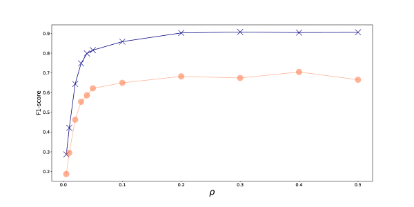
Figure 15: Mean $F_{1}$-score for identification step with respect to various values of $\rho$ on train and test set, respectively represented by the blue and pink curves.

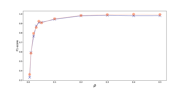
Figure 16: Mean $F_{1}$-score for localization step with respect to various values of $\rho$ on train and test set, respectively represented by the blue and pink curves.

To conclude on the sensitivity of the model performance to the amplitude of the anomaly shocks, although it is clear that a lower performance is observed on the identification and localization of smaller amplitude shock anomalies, the detection ratio is still satisfactory for this category of anomalies.

7 Application to a Downstream Task: Value-at-Risk Computations

In this section, we illustrate the benefit drawn when applying the PCA NN approach as a pre-processing before value-at-risk computations.

Given a random variable $\varrho$ representing the loss in portfolio position over a time horizon $h$, its value-at-risk at the confidence level $\alpha\in(\frac{1}{2},1)$, $\mathrm{VaR}_{\alpha}(\varrho)$, is defined by the quantile of level $\alpha$ of the loss distribution, i.e. $\mathbb{P}(\varrho\leq\mathrm{VaR}_{\alpha}(\varrho))=\alpha$ (assuming $\varrho$ atomless for simplicity). Let $(S_{t})_{t=t_{1},\ldots,t_{T}}$ be a path price diffusion distributed according to the Black-Scholes model (7). The logarithmic returns to maturity are distributed according to the Gaussian distribution

$$\ln\left(\frac{S_{t+h}}{S_{t}}\right)\sim\mathcal{N}\left(\left(\mu-\frac{\sigma^{2}}{2}\right)h,\sigma^{2}h\right),$$ (14)

with $\mu\in\mathbb{R}$ and $\sigma>0$.

We assume the vector $\bm{R}$ of log-returns on our stocks to be joint-normal,

$$\bm{R}=\left(R^{1},R^{2},\ldots,R^{i},\ldots,R^{N}\right)^{\top}\sim\mathcal{N}_{N}\left(\mu_{R},\Sigma_{R}\right),$$

where $R^{i}=\log\left(\frac{S^{i}_{t+h}}{S^{i}_{t}}\right)\sim\mathcal{N}\left(\mu_{i,R},\sigma_{i,R}^{2}\right)$ and $\Sigma_{R}$ is the covariance matrix.

We consider a portfolio on $N$ stocks, which return is given by $P=\mathcal{Q}^{\top}\bm{R}$, where $\mathcal{Q}\in\mathbb{R}^{N}$ defines the composition of the portfolio. Hence, $P\sim\mathcal{N}\left(\mu_{P},\sigma_{P}^{2}\right)$, where $\mu_{P}=\mathcal{Q}^{\top}\mu_{R}$ and $\sigma_{P}^{2}=\mathcal{Q}^{\top}\Sigma_{R}\mathcal{Q}$. The value-at-risk for the time horizon $h$ at level $\alpha$ is

$$\mathrm{VaR}_{\alpha}(P)=\mu_{P}+q_{\alpha}\sigma_{P}\;,$$ (15)

where $q_{\alpha}$ is the $\alpha$-quantile of a standard normal distribution and the parameters $\mu_{R}$ and $\Sigma_{R}$ are estimated from different types of time series to evaluate the impact of localizing and removing anomalies following our approach.

Under the adopted framework, the true $\mathrm{VaR}_{\alpha}(P)$, $\mathrm{VaR}^{theo}$ is thus known and can be computed using the diffusion parameters. An estimation $\widehat{\mathrm{VaR}}_{\alpha}(P)$ can be obtained by replacing the parameters in (15) by their estimates $\widehat{\mu_{P}}$ and $\widehat{\sigma_{P}}$ computed from the time series with anomalies, or after imputation of anomalies. Then, absolute errors and relative errors are computed as

$$\text{AbsoluteError}_{\text{VaR}}=\left\lvert\mathrm{VaR}_{\alpha}(P)-\widehat{\mathrm{VaR}}_{\alpha}(P)\right\rvert,$$

$$\text{RelativeError}_{\text{VaR}}=\frac{\left\lvert\mathrm{VaR}_{\alpha}(P)-\widehat{\mathrm{VaR}}_{\alpha}(P)\right\rvert}{\mathrm{VaR}_{\alpha}(P)}$$

Table 17 summarizes the four VaR estimations we consider in the sequel:

VaR estimation Name	$\widehat{\mu_{R}},\widehat{\Sigma_{R}}$ estimated on
$\mathrm{VaR}^{clean}$	Time series without anomalies
$\mathrm{VaR}^{anom}$	Times series with anomalies
$\mathrm{VaR}^{loc,true}$	Time series after anomalies imputation knowing their true localization
$\mathrm{VaR}^{loc,pred}$	Time series after anomalies imputation based on predicted localization

Table 17: Notations of VaR estimation based on the time series the VaR parameters have been estimated from.

To conduct this analysis, we generate new stock path samples that we assume to be clean, fixing the diffusion parameters $\mu_{R}$ and $\Sigma_{R}$. We then add the anomalies following the procedure described in Section 3. We apply our model to localize the anomalies and replace the localized anomalies using the backward fill (BF) approach (shown to be the more efficient imputation technique in Section 6.1). For each stock and each run of simulation, we obtain four estimates of the distribution parameters of the associated log-returns.

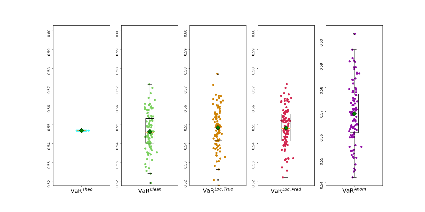
Figure 17: Boxplot representation of parametric VaR estimations for $P$. The green square represents the mean of VaR estimation.

VaR	$\mathrm{VaR}^{theo}$	$\mathrm{VaR}^{clean}$	$\mathrm{VaR}^{loc,true}$	$\mathrm{VaR}^{loc,pred}$	$\mathrm{VaR}^{anom}$
Mean	0.546851	0.546300	0.548392	0.548270	0.569015
Standard Deviation	0.0	0.010105	0.010739	0.010832	0.012268

Table 18: Summary of VaR estimations for $P$.

Figure 17 and Table 18 summarize the distribution of the VaR estimates for $\alpha=0.99$ and $h=1(day)$, over several simulation runs. The boxplots show the dispersion of the portfolio VaR estimates on several diffusions. The green square represents the mean of the VaR estimates. For the four first boxplots, the means are approximately on the same level, which is confirmed by the results of Table 18. The anomalies present among the time series observed values have a non-negligible impact on the distribution parameters estimation, which ultimately causes a wrong estimation of the VaR. Thanks to the localization of the anomalies by the suggested model and their imputation as per Section 6.1, we are able to get a more accurate estimation of the VaR. $\mathrm{VaR}^{loc,true}$ and $\mathrm{VaR}^{loc,pred}$ are quite similar, which shows that the model accurately localizes the anomalies.

VaR	$\mathrm{VaR}^{clean}$	$\mathrm{VaR}^{loc,true}$	$\mathrm{VaR}^{loc,pred}$	$\mathrm{VaR}^{anom}$
Absolute Error	0.007995	0.008596	0.008622	0.02235
Relative Error	0.014620	0.015720	0.015767	0.04087

Table 19: Mean absolute and relative error on VaR estimations for $P$.

We also evaluate the error on the VaR estimation using the mean absolute error and the mean relative error, taking the $\mathrm{VaR}^{theo}$ as our benchmark. As one can tell from Table 19, even when the distribution parameters are estimated from the clean time series, the VaR computed with these parameters is not exactly the one computed with the theoretical parameters. This can be explained by the historical size of the observed values used to estimate the parameters. This table shows that by removing anomalies we can reduce by a factor two the error on VaR estimation.

Additionally, we assess the impact on $\mathrm{VaR}^{theo},\mathrm{VaR}^{clean},\mathrm{VaR}^{anom},\mathrm{VaR}^{loc,true}$ and $\mathrm{VaR}^{loc,pred}$ of increasing $n^{anom}$. To this end, we perform 50 simulation runs of stock paths for $n^{anom}$ and for each of those scenarios we estimate the VaR on the portfolio. We summarize the results on Figure 18, where each curve represents the mean VaR estimation with respect to $n^{anom}$ along with a representation of the uncertainty around each evaluated point through a confidence interval.

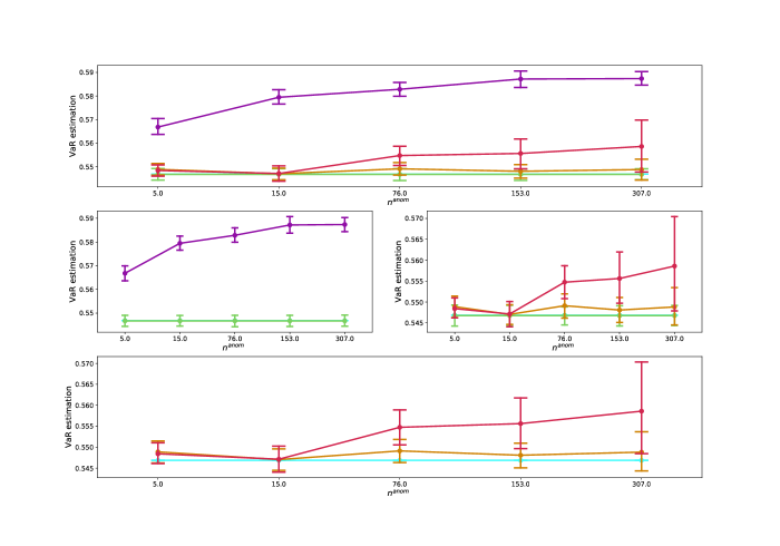
Figure 18: VaR estimation based on parameter estimation from time series with and without anomalies (purple and light blue curves), time series after localization and imputation of anomalies with the suggested approach (red curve) and time series imputed knowing the true localization of the anomalies (brown curve), with respect to $n^{anom}$.

When we compute the VaR using the abnormal time series, we notice that the difference between $\mathrm{VaR}^{anom}$ and $\mathrm{VaR}^{theo}$ increases with $n^{anom}$, which is natural to expect. However, when the time series are cleaned prior to VaR estimation, the curve representing the VaR estimates are much closer to the ones representing $\mathrm{VaR}^{theo}$ and $\mathrm{VaR}^{clean}$, showing an undeniable improvement in the accuracy of the VaR estimation over the estimation based on abnormal time series. Furthermore, VaR estimation after the imputation following the model prediction or knowing the true localization of the anomalies seem to be quite similar for low $n^{anom}$, while some discrepancies between the two become more significant as $n^{anom}$ increases. A natural explanation could be that when the number of anomalies increases and the model suggests wrong anomalies localization, normal values are being replaced while true anomalies remain among the observed values, which wrongly impacts the VaR estimation. However, the results of Tables 20 and 21 indicate that the anomaly localizations suggested by the model are overall correct and allow removing most of the anomalies, as the relative error of $\mathrm{VaR}^{loc,pred}$ is, regardless of $n^{anom}$, always lower than the relative error of $\mathrm{VaR}^{anom}$ (e.g a relative error of 0.0248 for $\mathrm{VaR}^{loc,pred}$, against 0.0658 for $\mathrm{VaR}^{anom}$, when there are $76$ anomalies among the $1,500$ observed values of the time series).

$n^{anom}$	$\mathrm{VaR}^{clean}$	$\mathrm{VaR}^{loc,true}$	$\mathrm{VaR}^{loc,pred}$	$\mathrm{VaR}^{anom}$
5	0.012194	0.013796	0.013341	0.037392
15	0.012194	0.012623	0.016676	0.059604
76	0.012194	0.014831	0.024807	0.065791
153	0.012194	0.014644	0.034361	0.073750
307	0.012194	0.020537	0.052244	0.074091

Table 20: Mean relative error of parametric VaR estimations with respect to $n^{anom}$, for parameters estimated from clean time series, time series with anomalies, imputed time series following predicted location ($\mathrm{VaR}^{loc,pred}$) and true anomalies localization ($\mathrm{VaR}^{loc,true}$).

$n^{anom}$	$\mathrm{VaR}^{clean}$	$\mathrm{VaR}^{loc,true}$	$\mathrm{VaR}^{loc,pred}$	$\mathrm{VaR}^{anom}$
5	0.010356	0.011511	0.009678	0.020674
15	0.010356	0.010514	0.012723	0.020172
76	0.010356	0.011842	0.018696	0.019930
153	0.010356	0.013683	0.026117	0.024243
307	0.010356	0.022526	0.057903	0.019207

Table 21: Standard deviation of relative error of parametric VaR estimations with respect to $n^{anom}$, for parameters estimated from clean time series, time series with anomalies, imputed time series following predicted location ($\mathrm{VaR}^{loc,pred}$) and true anomalies localization ($\mathrm{VaR}^{loc,true}$).

8 Numerical Results on Real Data

We consider a labelled real data set including stock prices, bonds yields, CDS spreads, FX rates, and volatilities. These data were collected from a financial data provider for the period between 2018 and 2020. These data sets were labelled by experts. They are provided on https://github.com/MadharNisrine/PCANN in the form of 132,000 time series (after augmentation). The train set is balanced, while the test set is imbalanced with 20% of contaminated time series.

To ensure the independence of the train and test data sets, we calibrate the PCA NN approach considering the time series of 2018 and 2019, while the 2020 time series are dedicated to model evaluation. The performance evaluation of the PCA NN approach after its calibration on real data sets is shown in Table 22. As visible from the upper panel, the PCA NN performs quite well for the identification step. Once the contaminated time series are identified, the model is able to localize the anomaly with high accuracy, as reflected by the scores on the test set in the lower panel.

Data set Accuracy Precision Recall $F_{1}$-score Train set 92.88 % 99.17% 86.49% 92.40% Test set 88.15% 72.45% 46.10% 56.35%

Data set Accuracy Precision Recall $F_{1}$-score Train set 99.48 % 99.49% 99.48% 99.48% Test set 96.05% 96.21% 96.05% 95.92%

Table 22: Performance of the PCA NN identification step (upper part) and localization step (lower part) on the real data set.

8.1 PCA NN against State of the Art Models on Real Data

Even if the $F_{1}$-score on the identification step is not that high, the results show that the related performance remains better than the one of alternative state of the art approaches.

Tables 23 and 24 compare the performance of the PCA NN approach against the state of the art models of Section B on our real data set. PCA NN outperforms the benchmark models in both steps, with overwhelming results for the anomaly localization step.

Model	Accuracy	Precision	Recall	$F_{1}$-score
IF	73.17%	18.12%	17.53%	17.82%
LOF	82.33%	44.57%	26.62%	33.33%
DBSCAN	22.74%	15.71%	83.77%	26.46%
sig-IF	73.34%	18.15%	17.47%	17.80%
KNN	70.26%	23.48%	35.06%	28.13%
SVM	50.11%	24.46%	96.10%	39.00%
PCA NN	88.15%	72.45%	46.10%	56.35%

Table 23: Performance evaluation of unsupervised (upper part) and supervised (lower part) models for contaminated time series identification step.

Model	Accuracy	Precision	Recall	$F_{1}$-score
IF	78.50%	2.173%	98.35%	4.252%
LOF	87.04%	0.3713%	9.616%	0.7151%
DBSCAN	N/A	N/A	N/A	N/A
sig-IF	N/A	N/A	N/A	N/A
KNN	99.85%	78.38%	95.59%	86.13%
SVM	N/A	N/A	N/A	N/A
PCA NN	96.05%	96.21%	96.05%	95.92%

Table 24: Performance evaluation of unsupervised (upper part) and supervised (lower part) models for contaminated time series localization step. Results for DBSCAN, sig-IF and SVM are not provided due to high computational cost.

9 Conclusion

We propose a two step approach for detecting anomalies on a panel of time series that can reflect a wide variety of market risk factors. The first step aims at identifying the contaminated time series, i.e. time series with anomalies. The second step focuses on the localization of the anomaly among the observed values of the identified contaminated time series. As preprocessing, our methodology integrates the extraction of features from the time series with PCA. This part of the method proves to be essential, as it provides the models with inputs on which the distinction between abnormal/contaminated and normal instances is eased, while also ensuring the stationarity of the model (time series) inputs. Another key point of the approach is the calibration of the cut-off value, the key parameter in the identification of contaminated time series, by means of a feedforward neural network with a customized loss function. The proposed approach suggests an imputation value, however this value is strongly influenced by the abnormal value. Therefore, basic imputation approaches with similar complexity are preferred. Our numerical experiments show not only that our approach outperforms baseline anomaly detection models, but also show the real benefit that could be gained from applying it as a data cleaning step preliminary to VaR computations. Future research could focus on the replacement of PCA by partial least squares (PLS) or deep PLS (Polson et al., 2021) for endogeniging the features extraction stage. Regarding downstream tasks, our approach might be of special interest for reverse stress tests (Eichhorn et al., 2021).

Appendix A Literature Review

We start with a review of the anomaly detection literature. See also Section B for a more technical presentation of some of the below-mentioned algorithms.

A.1 Baseline Algorithms

Anomaly detection aims at finding an “observation that deviates so much from other observations as to arouse suspicion that it was generated by a different mechanism" (Hawkins, 1980). The baseline anomaly detection algorithms, described in (Chandola, 2009), struggle to identify anomalies in time series, mainly because their assumptions are invalidated. If we consider models built for spatial data, a major assumption of these models is that observations are independent, whereas, for time series, high dependency exists between different time stamps. Clustering-based approaches, like the density based spatial clustering with noise (DBSCAN) method, are particularly impacted by this aspect: if an anomaly occurs at a given time stamp and is followed by incorrect values, clustering-based approaches consider that the observations of the time series belong to two different clusters and thus fail to identify the anomaly. Another limitation when considering this type of techniques is the choice of the similarity metric used for data clustering. This task, although being a crucial pillar of these approaches, is not trivial and becomes very challenging for high dimensional problems.

A.2 Statistical Approach to Anomaly Detection

The statistical techniques for anomaly detection can be split in two families: statistical tests and predictive models. Both suffer from the curse of dimensionality and model/data mismatch. When anomaly detection relies on hypothesis tests, it usually tests whether the observations are drawn from a known distribution (Zhang and Paschalidis, 2017), supposing that the user knows the probability distribution of the normal observations. Such a parametric framework narrows down the scope of applicability of hypothesis tests, as the data does not always coincide with the assumed distribution. Moreover, the tests provided in the literature are not suitable in multivariate settings (Kurt et al., 2020). The statistical techniques relying on fitting a predictive model to each time series also require strong assumptions on the data. Predictive models are usually autoregressive (AR), moving average (MA), or ARMA models. Anomalies are then detected relatively to the forecasts suggested by the model (Chandola, 2009). In these parametric approaches, some parameters have to be specified again, starting with the order of the models. Selecting the optimal model parameters with respect to an information criterion is not always possible. Additionally, these models assume that the time series are homogeneous, i.e. drawn from the same distribution (Laptev et al., 2015). This is not always satisfied in the financial risk management case where several types of market risk factors are treated simultaneously.

A.3 Score Based Anomaly Detection Models

Additional anomaly detection challenges are of general concern. Most of anomaly detection algorithms are score-based, in the sense that these approaches return an anomaly score reflecting to which extent the observation is considered to be abnormal by the model. In order to decide whether an observation is abnormal or not, a cut-off value of the score has to be selected. Empirical approaches are often used, consisting in setting the cut-off value as a quantile or elbow point of the distribution of the anomaly score. However, the selected cut-off value according to such methods remains arbitrary. (Gao and Tan, 2006) propose to rely on a cost of misclassification based on a weighted classification accuracy. Approaches to calculate “optimal” weights are described in (Lu et al., 2019), but they involve a heuristic grid search technique. Another alternative is to determine the cut-off value by cross validation on the training data (Saha et al., 2009). Finally, some methods do not select any cut-off value, but are based instead on a contamination rate. However, fixing a cut-off value or deciding on a contamination rate is not so different.

A.4 Scarcity of Anomalies and Data Augmentation

The scarcity of anomalies within the data sets is another typical problem in anomaly detection. Anomalies are, by definition, rare events, therefore they are under-represented in the data set used to fit the models. This under-representation is not helping in the design of a reliable model able to identify anomalies. Classical methods to overcome this issue consider data augmentation. These techniques aim at producing new synthetic samples that will ultimately enhance model performance, leveraging on a better representation of the features space. As reported in (Wen et al., 2020), time series can be augmented by using a simple transformation in time domain (Cui et al., 2016), frequency domain (Gao et al., 2020), or more advanced generative approaches involving deep learning techniques, such as recurrent generative adversarial networks (Esteban et al., 2017). In practice, the use of generative models for data augmentation of time series with anomalies presents two limitations. First, training such models requires a large number of samples to guarantee a satisfactory performance. While restricted Boltzman machines do not exhibit this problem, (Kondratyev et al., 2020) have shown that they fail into fitting multivariate complex distributions with nonlinear dependence structure. A more fundamental limitation affects the very idea behind generative models. Such networks are trained to learn a given distribution. However, by definition, anomalies are different from each other and therefore there is not a distribution that characterises them.

A.5 Supervised vs. Unsupervised learning

Since anomalies are the realisations of atypical events for which the distribution is unknown, it seems quite natural to use unsupervised algorithms. However, these approaches are deemed more suitable for learning complex patterns and are task specific. Moreover, (Görnitz et al., 2013) pointed out that they often do not present a high prediction performance, in particular in high dimensional settings (Ruff et al., 2019). Indeed, the performance of unsupervised shallow anomaly detection algorithms depends upon a features engineering step. (Akyildirim et al., 2022) use signatures to extract features which then feed algorithms such as isolation forest. This combination of techniques is shown to over-perform benchmark approaches. However, the designed model is task specific (detection of pump and dumps attacks) and the features extraction step is only efficient when at least one explanatory variable is considered in the analysis. Moreover, the unavailability of labelled data makes the model building and its evaluation even more complex. As for supervised methods, the only limitation on which the literature tends to agree is their incapacity to generalize the learned patterns to new samples, which is the consequence of misrepresentation of anomalies among the training samples (Zhao and Hryniewicki, 2018). However, the scarcity of labelled data can be sidestepped through the use of data augmentation techniques on the fraction of available labelled data. For these reasons the supervised learning framework is to be preferred even when only a small set of labelled data is available.

A.6 Anomaly Detection on Time Series

Usually, anomaly detection models on time series have two main components. The first component aims at extracting a parsimonious yet expressive representation of the time series. Several approaches are suggested in the literature to deal with such features extraction. Recently, deep neural networks have been shown to suffer from overparametrization and to be often computationally expensive (Dempster et al., 2020; Akyildirim et al., 2022). Path signatures are also computationally demanding. This could perhaps be alleviated by the random signatures (Compagnoni et al., 2022). However, the information extracted with signatures is of most interest when the considered paths are characterized by several variables. The resulting representation is then transformed into a (typically continuous) anomaly score which is in turn converted into a binary label (Braei and Wagner, 2020).

A.7 PCA and Anomaly Detection

In the literature, PCA is usually used in anomaly detection for its dimension reduction properties. Anomalies are identified on the latent space, either by applying some anomaly detection algorithm or by assuming a given distribution on the principal component and identifying the anomalies relatively to a quantile (Shyu et al., 2006). Assuming that a normal subspace representation of the data set can be constructed with the first $k$-components (Ringberg et al., 2007), anomaly detection is achieved by looking at the observations that cannot be expressed in terms of the first $k$-components (Bin et al., 2016). Note that the particular power-fullness of auto-encoder, a non-linear PCA, as data compressor is not desirable herein, since auto-encoders compress all patterns including abnormal ones. While (Ding and Tian, 2016) claimed that the PCA-based models are stable with respect to their parameters, such as the number of principal components $k$ spanning the subspace or the cut-off level, (Ringberg et al., 2007) found instead that PCA-based anomaly detection is sensitive to these parameters and to the amplitude of the anomalies. Indeed, the latter may undermine the construction of the normal subspace representation, in turn leading to misidentification of anomalies. In light of that, we take an extra care regarding these aspects, and appropriate tests are conducted to show that the proposed approach is not subject to these issues. In the end, with a relatively low number of features given by PCA, we are able to accurately describe the dynamics of market risk factors represented by times series. The reason standing behind that is the high correlation structure displayed by market risk factors.

Appendix B State of the Art Anomaly Detection Models

There are mainly two categories of machine learning anomaly detection models : density-based models, where a distribution is used to fit the data and anomalies are defined relatively to this distribution, and depth-based models, which, instead of modeling the normal behaviour, isolate anomalies.

B.1 Density-Based Models

Density based spatial clustering with noise (DBSCAN)

DBSCAN (Ester et al., 1996; Schubert et al., 2017) is an unsupervised clustering methodology that groups together comparable observations based on a similarity metric. Clusters are high density regions and are defined by the $\varepsilon$-neighbourhood of observations and by MinPts, the minimum number of points required to be in a radius of $\varepsilon$ from an observation to form a dense region. An anomaly is any observation which has not $MinPts$ in its $\varepsilon$-neighbourhood nor appears in the $\varepsilon$-neighbourhood of other observations.

K-nearest neighbours (KNN)

Usually used for classification purposes, KNN (Hand, 2007) is a supervised algorithm that can be used for anomaly detection as well. For each observation it selects its closest $K$ observations generally in terms of distance, but other similarity metrics can be considered. The anomaly score of an observation is computed as function of its distances to $K$-nearest neighbours, weighted average of the distances for instance. The points with the highest anomaly scores are considered as anomalies.

Support Vector Machines (SVM)

The ultimate aim of SVM (Cortes and Vapnik, 1995) is to define a hyperplan that separates the data. The specificity of this hyperplan is that it maximizes the distances to the set of features representing each class. When the data is not linearly separable, a map $\phi$ is applied to the initial features vector so the data became linearly separable in the new space in which it was projected.

B.2 Depth-Based Models

Isolation Forest (IF)

The IF method (Hariri et al., 2019) applies a depth approach to detect anomalies. The algorithm is based on the idea that anomalies are easier to isolate and thus will be isolated closer to the root, while normal observations are isolated much further from the root. The algorithm uses random decision trees to separate the observations. The anomaly score is calculated as the path length to isolate the observation. As it is defined in the algorithm, the anomaly score will be closer to 1 for anomalies and $\ll 1$ for normal observations. This allows ranking the observations, from the most abnormal observation to the most regular one. However, the choice of an explicit cut-off between this two type of instances is not obvious.

Local Outlier Factor (LOF)

The LOF algorithm (Breunig et al., 2000; Alghushairy et al., 2020) tries to assess the isolation of one observation relatively to the rest of the data set, before flagging it as an anomaly. This model relies on the concept of local density. The anomaly score of an observation $x$ is its local outlier factor, which quantifies how dense is the location area of $x$ compared to the one of its neighbours. Hence, for each observation, $\mathrm{LOF}_{k}(x)\approx 1$ means that the density of observations around $x$ is similar to the one of its neighbours, therefore $x$ could not be considered as an isolated observation. $\mathrm{LOF}_{k}(x)\gg 1$, instead, shows that the density of $x$ is lower compared to its neighbours, hence $x$ should be flagged as anomaly

Appendix C The Data Stationary Issue

Assume that a process $\left(\varepsilon^{i}_{t}\right)$ satisfies the following representation

$$\Delta\varepsilon^{i}_{t}=\gamma\varepsilon^{i}_{t-1}+\theta_{1}\Delta\varepsilon^{i}_{t-1}+\dots+\theta_{p-1}\Delta\varepsilon^{i}_{t-p+1}+z_{t},$$

where $p$ is the lag order, $\Delta$ is the difference operator, i.e $\Delta\varepsilon_{t}=\varepsilon_{t}-\varepsilon_{t-1}$, and $z_{t}$ is a white noise. The stationarity of $(\varepsilon^{i}_{t})$ is shown using the augmented Dickey-Fuller test (Fuller, 2009). Namely, the process $\varepsilon^{i}$ is stationary if there is a unit root, i.e. $\gamma=0$. Therefore, for each $\varepsilon^{i}$ the test is carried under the null hypothesis $\mathcal{H}_{0}:\gamma=0\;\text{against}\;\mathcal{H}_{1}:\gamma<0$.

Set	Mean	Standard dev.	Min	25%	50%	75%	Max
Train	1.26e-14	1.74e-13	6.63e-24	3.46e-20	1.92e-18	3.74e-17	3.88e-12
Test	1.51e-14	4.83-13	6.20e-30	4.23e-19	8.45e-18	1.65e-16	4.35e-11

Table 25: Descriptive statistics on p-values for train and test set time series $\bm{\varepsilon}$.

If the p-values are lower than the significance level, then the null hypothesis is rejected for all the reconstruction errors and we conclude that the time series we work with do not suffer from the non-stationarity issue.

References

- Aggarwal et al. (2001) Aggarwal, C. C., A. Hinneburg, and D. A. Keim (2001). On the surprising behavior of distance metrics in high dimensional space. In International conference on database theory, pp. 420–434. Springer.
- Ahmed et al. (2016) Ahmed, M., A. N. Mahmood, and J. Hu (2016). A survey of network anomaly detection techniques. Journal of Network and Computer Applications 60, 19–31.
- Akyildirim et al. (2022) Akyildirim, E., M. Gambara, J. Teichmann, and S. Zhou (2022). Applications of signature methods to market anomaly detection. arXiv:2201.02441.
- Alghushairy et al. (2020) Alghushairy, O., R. Alsini, T. Soule, and X. Ma (2020). A review of local outlier factor algorithms for outlier detection in big data streams. Big Data and Cognitive Computing 5(1), 1.
- Ali et al. (2019) Ali, H., M. N. M. Salleh, R. Saedudin, K. Hussain, and M. F. Mushtaq (2019). Imbalance class problems in data mining: A review. Indonesian Journal of Electrical Engineering and Computer Science 14(3), 1560–1571.
- Basel Committee on Banking Supervision (2013) Basel Committee on Banking Supervision (2013). Consultative document: Fundamental Review of the Trading Book: A revised market risk framework.
- Bengio et al. (2017) Bengio, Y., I. Goodfellow, and A. Courville (2017). Deep learning, Volume 1. MIT press Cambridge, MA, USA.
- Bin et al. (2016) Bin, X., Y. Zhao, and B. Shen (2016). Abnormal subspace sparse PCA for anomaly detection and interpretation. arXiv:1605.04644.
- Braei and Wagner (2020) Braei, M. and S. Wagner (2020). Anomaly detection in univariate time-series: A survey on the state-of-the-art. arXiv:2004.00433.
- Breunig et al. (2000) Breunig, M. M., H.-P. Kriegel, R. T. Ng, and J. Sander (2000). LOF: identifying density-based local outliers. In Proceedings of the 2000 ACM SIGMOD international conference on Management of data, pp. 93–104.
- Brownlee (2020) Brownlee, J. (2020). Imbalanced Classification with Python: Better Metrics, Balance Skewed Classes, Cost-Sensitive Learning. Machine Learning Mastery.
- Chandola (2009) Chandola, V. (2009). Anomaly detection for symbolic sequences and time series data. Ph. D. thesis, University of Minnesota.
- Chataigner et al. (2020) Chataigner, M., S. Crépey, and J. Pu (2020). Nowcasting networks. Journal of Computational Finance 24(3), pages 1–39.
- Chen (2017) Chen, Y.-C. (2017). A tutorial on kernel density estimation and recent advances. Biostatistics & Epidemiology 1(1), 161–187.
- Cheng et al. (2019) Cheng, Y., I. Diakonikolas, R. Ge, and D. Woodruff (2019). Faster algorithms for high-dimensional robust covariance estimation. arXiv:1906.04661.
- Chinchor and Sundheim (1993) Chinchor, N. and B. M. Sundheim (1993). MUC-5 evaluation metrics. In Fifth Message Understanding Conference (MUC-5): Proceedings of a Conference Held in Baltimore, Maryland, August 25-27, 1993.
- Compagnoni et al. (2022) Compagnoni, E. M., L. Biggio, A. Orvieto, T. Hofmann, and J. Teichmann (2022). Randomized signature layers for signal extraction in time series data. arXiv:2201.00384.
- Cortes and Vapnik (1995) Cortes, C. and V. Vapnik (1995). Support-vector networks. Machine learning 20(3), 273–297.
- Cui et al. (2016) Cui, Z., W. Chen, and Y. Chen (2016). Multi-scale convolutional neural networks for time series classification. arXiv:1603.06995.
- Dempster et al. (2020) Dempster, A., F. Petitjean, and G. I. Webb (2020). Rocket: exceptionally fast and accurate time series classification using random convolutional kernels. Data Mining and Knowledge Discovery 34(5), 1454–1495.
- Ding and Tian (2016) Ding, M. and H. Tian (2016). PCA-based network traffic anomaly detection. Tsinghua Science and Technology 21(5), 500–509.
- Eichhorn et al. (2021) Eichhorn, M., T. Bellini, and D. Mayenberger (2021). Reverse Stress Testing in Banking: A Comprehensive Guide. De Gruyter.
- Esteban et al. (2017) Esteban, C., S. L. Hyland, and G. Rätsch (2017). Real-valued (medical) time series generation with recurrent conditional gans. arXiv:1706.02633.
- Ester et al. (1996) Ester, M., H.-P. Kriegel, J. Sander, X. Xu, et al. (1996). A density-based algorithm for discovering clusters in large spatial databases with noise. In kdd, Volume 96, pp. 226–231.
- Fuller (2009) Fuller, W. A. (2009). Introduction to statistical time series. Wiley.
- Gao et al. (2020) Gao, J., X. Song, Q. Wen, P. Wang, L. Sun, and H. Xu (2020). Robusttad: Robust time series anomaly detection via decomposition and convolutional neural networks. arXiv:2002.09545.
- Gao and Tan (2006) Gao, J. and P.-N. Tan (2006). Converting output scores from outlier detection algorithms into probability estimates. In Sixth International Conference on Data Mining (ICDM 06), pp. 212–221. IEEE.
- Goodfellow et al. (2016) Goodfellow, I., Y. Bengio, and A. Courville (2016). Deep learning. MIT press.
- Görnitz et al. (2013) Görnitz, N., M. Kloft, K. Rieck, and U. Brefeld (2013). Toward supervised anomaly detection. Journal of Artificial Intelligence Research 46, 235–262.
- Halko et al. (2011) Halko, N., P.-G. Martinsson, and J. A. Tropp (2011). Finding structure with randomness: Probabilistic algorithms for constructing approximate matrix decompositions. SIAM review 53(2), 217–288.
- Hand (2007) Hand, D. J. (2007). Principles of data mining. Drug safety 30(7), 621–622.
- Hariri et al. (2019) Hariri, S., M. C. Kind, and R. J. Brunner (2019). Extended isolation forest. IEEE Transactions on Knowledge and Data Engineering 33(4), 1479–1489.
- Hawkins (1980) Hawkins, D. M. (1980). Identification of outliers. Springer.
- Henry-Labordère (2019) Henry-Labordère, P. (2019). Optimal transport and anomaly detection with neural networks: A primal-dual algorithm. ssrn:3370910.
- Hyndman et al. (2015) Hyndman, R. J., E. Wang, and N. Laptev (2015). Large-scale unusual time series detection. In 2015 IEEE international conference on data mining workshop (ICDMW), pp. 1616–1619. IEEE.
- Jolliffe (2003) Jolliffe, I. T. (2003). Principal component analysis. Technometrics 45(3), 276.
- Kingma and Ba (2014) Kingma, D. P. and J. Ba (2014). Adam: A method for stochastic optimization. arXiv:1412.6980.
- Kondratyev et al. (2020) Kondratyev, A., C. Schwarz, and B. Horvath (2020). Data anonymisation, outlier detection and fighting overfitting with restricted Boltzmann machines. ssrn:3526436.
- Kriegel et al. (2008) Kriegel, H.-P., M. Schubert, and A. Zimek (2008). Angle-based outlier detection in high-dimensional data. In Proceedings of the 14th ACM SIGKDD international conference on knowledge discovery and data mining, pp. 444–452.
- Kurt et al. (2020) Kurt, M. N., Y. Yılmaz, and X. Wang (2020). Real-time nonparametric anomaly detection in high-dimensional settings. IEEE transactions on pattern analysis and machine intelligence 43(7), 2463–2479.
- Kwon et al. (2019) Kwon, D., H. Kim, J. Kim, S. C. Suh, I. Kim, and K. J. Kim (2019). A survey of deep learning-based network anomaly detection. Cluster Computing 22(1), 949–961.
- Laptev et al. (2015) Laptev, N., S. Amizadeh, and I. Flint (2015). Generic and scalable framework for automated time-series anomaly detection. In Proceedings of the 21th ACM SIGKDD international conference on knowledge discovery and data mining, pp. 1939–1947.
- Le Guennec et al. (2016) Le Guennec, A., S. Malinowski, and R. Tavenard (2016). Data augmentation for time series classification using convolutional neural networks. In ECML/PKDD workshop on advanced analytics and learning on temporal data.
- Linting et al. (2007) Linting, M., J. J. Meulman, P. J. Groenen, and A. J. van der Koojj (2007). Nonlinear principal components analysis: introduction and application. Psychological methods 12(3), 336.
- Lu et al. (2019) Lu, H., Y. Xu, M. Ye, K. Yan, Z. Gao, and Q. Jin (2019). Learning misclassification costs for imbalanced classification on gene expression data. BMC bioinformatics 20(25), 1–10.
- Munawar et al. (2017) Munawar, A., P. Vinayavekhin, and G. De Magistris (2017). Limiting the reconstruction capability of generative neural network using negative learning. In 2017 IEEE 27th International Workshop on Machine Learning for Signal Processing (MLSP), pp. 1–6. IEEE.
- Mushtaq (2011) Mushtaq, R. (2011). Augmented Dickey-Fuller test. ssrn:1911068.
- Polson et al. (2021) Polson, N., V. Sokolov, and J. Xu (2021). Deep learning partial least squares. arXiv:2106.14085.
- Ringberg et al. (2007) Ringberg, H., A. Soule, J. Rexford, and C. Diot (2007). Sensitivity of pca for traffic anomaly detection. In SIGMETRICS international conference on measurement and modeling of computer systems, pp. 109–120.
- Ruff et al. (2019) Ruff, L., R. A. Vandermeulen, N. Görnitz, A. Binder, E. Müller, K.-R. Müller, and M. Kloft (2019). Deep semi-supervised anomaly detection. arXiv:1906.02694.
- Saha et al. (2009) Saha, B. N., N. Ray, and H. Zhang (2009). Snake validation: A PCA-based outlier detection method. IEEE signal processing letters 16(6), 549–552.
- Sahoo et al. (2021) Sahoo, R., S. Zhao, A. Chen, and S. Ermon (2021). Reliable decisions with threshold calibration. Advances in Neural Information Processing Systems 34, 1831–1844.
- Saito and Rehmsmeier (2015) Saito, T. and M. Rehmsmeier (2015). The precision-recall plot is more informative than the ROC plot when evaluating binary classifiers on imbalanced datasets. PloS one 10(3), e0118432.
- Schubert et al. (2017) Schubert, E., J. Sander, M. Ester, H. P. Kriegel, and X. Xu (2017). DBSCAN revisited, revisited: why and how you should (still) use DBSCAN. ACM Transactions on Database Systems (TODS) 42(3), 1–21.
- Shyu et al. (2006) Shyu, M.-L., S.-C. Chen, K. Sarinnapakorn, and L. Chang (2006). Principal component-based anomaly detection scheme. In Foundations and novel approaches in data mining, pp. 311–329. Springer.
- Um et al. (2017) Um, T. T., F. M. Pfister, D. Pichler, S. Endo, M. Lang, S. Hirche, U. Fietzek, and D. Kulić (2017). Data augmentation of wearable sensor data for parkinson’s disease monitoring using convolutional neural networks. In Proceedings of the 19th ACM international conference on multimodal interaction, pp. 216–220.
- Van Rijsbergen (1979) Van Rijsbergen, C. (1979). Information retrieval: theory and practice. In Proceedings of the Joint IBM/University of Newcastle upon Tyne Seminar on Data Base Systems, Volume 79.
- Węglarczyk (2018) Węglarczyk, S. (2018). Kernel density estimation and its application. In ITM Web of Conferences, Volume 23(2):00037. EDP Sciences.
- Wen et al. (2020) Wen, Q., L. Sun, F. Yang, X. Song, J. Gao, X. Wang, and H. Xu (2020). Time series data augmentation for deep learning: A survey. arXiv:2002.12478.
- (60) Yu, Y., Y. Zhu, S. Li, and D. Wan. Time series outlier detection based on sliding window prediction. Mathematical Problems in Engineering 2014, 1–14.
- Zhang et al. (2012) Zhang, J., J. Erway, X. Hu, Q. Zhang, and R. Plemmons (2012). Randomized SVD methods in hyperspectral imaging. J. Elect Comput. Eng. 2012, 1–15.
- Zhang and Paschalidis (2017) Zhang, J. and I. C. Paschalidis (2017). Statistical anomaly detection via composite hypothesis testing for markov models. arXiv:1702.08435.
- Zhao and Hryniewicki (2018) Zhao, Y. and M. K. Hryniewicki (2018). XGBOD: improving supervised outlier detection with unsupervised representation learning. In 2018 International Joint Conference on Neural Networks (IJCNN), pp. 1–8.