Mixedness timescale in non-Hermitian quantum systems

Abstract

We discuss the short-time perturbative expansion of the linear entropy for finite-dimensional quantum systems whose dynamics can be effectively described by a non-Hermitian Hamiltonian. We derive a timescale for the degree of mixedness for an input state undergoing non-Hermitian dynamics and specialize these results in the case of a driven-dissipative two-level system. Next, we derive a timescale for the growth of mixedness for bipartite quantum systems that depends on the effective non-Hermitian Hamiltonian. In the Hermitian limit, this result recovers the perturbative expansion for coherence loss in Hermitian systems, while it provides an entanglement timescale for initial pure and uncorrelated states. To illustrate these findings, we consider the many-body transverse-field $XY$ Hamiltonian coupled to an imaginary all-to-all Ising model. We find that the non-Hermitian Hamiltonian enhances the short-time dynamics of the linear entropy for the considered input states. Overall, each timescale depends on minimal ingredients such as the probe state and the non-Hermitian Hamiltonian of the system, and its evaluation requires low computational cost. Our results find applications to non-Hermitian quantum sensing, quantum thermodynamics of non-Hermitian systems, and $\mathcal{PT}$-symmetric quantum field theory.

I Introduction

The study of non-Hermitian systems Brody and Graefe (2012); Roccati et al. (2022) has paved the way for recent developments across the subjects of quantum sensing Yu et al. (2020); Wang et al. (2021), $\mathcal{PT}$ symmetry and exceptional points Zyablovsky et al. (2016); Kawabata et al. (2017); Delplace et al. (2021); Ashida et al. (2020); Bergholtz et al. (2021); Shackleton and Scheurer (2020); Tzeng et al. (2021); Lourenço et al. (2022), linear response theory Sticlet et al. (2022), quantum many-body systems Korff and Weston (2007); Korff (2008); Castro-Alvaredo and Fring (2009); Ashida et al. (2017); Xiao et al. (2019); Lee et al. (2020); Hamazaki et al. (2019); Matsumoto et al. (2020); Takasu et al. (2020); Turkeshi and Schiró (2023); Gal et al. (2022), skin effect Kawabata et al. (2020); Peng et al. (2022); Žnidarič (2022), bulk-edge correspondence Yao and Wang (2018); Yang et al. (2020), phase transitions Pará et al. (2021); Nakanishi and Sasamoto (2022), and the quantum boomerang effect in localized systems Noronha et al. (2022); Sajjad et al. (2022); Prat et al. (2019); Noronha and Macrì (2022), to cite a few.

Recent theoretical achievements discussed the effects of postselection on the dynamics of open quantum systems, thus reconciling the approaches of effective non-Hermitian Hamiltonians and Liouvillian superoperators Minganti et al. (2019, 2020). In this setting, several works have addressed the role of non-Hermitian features on legitimate quantum mechanical signatures, e.g., quantum coherence and entanglement Pires and Macrì (2021); Huang et al. (2021); Gopalakrishnan and Gullans (2021); Chen et al. (2022a); Fang et al. (2022). For example, it has been shown that quantum coherence can be characterized under the framework of multiple quantum coherences Ortega-Taberner et al. (2022); Macieszczak et al. (2019); Pires et al. (2020). In turn, the dynamics of entanglement in non-Hermitian systems has been widely probed with entropic measures, but their evaluation generally involves the full spectral decomposition of the state driven by the non-Hermitian Hamiltonian Sergi and Zloshchastiev (2016); Zhang et al. (2017); Guo et al. (2021); Chen et al. (2022b). This can be a challenging computational task, especially for interacting quantum many-body systems.

To overcome this issue, the onset growth of mixedness at earlier times of the dynamics can be addressed through the so-called linear entropy, a useful information-theoretic quantifier that is related to the second-order Rényi entropy and quantum purity Li et al. (2017); Streltsov et al. (2018). Remarkably, those quantities have been experimentally probed in optical lattices Islam et al. (2015); Elben et al. (2018); Kaufman et al. (2016), and trapped ion setups Linke et al. (2018); Brydges et al. (2019). In the Hermitian case, it is known that the short-time perturbative expansion of the linear entropy implies a universal timescale for the entanglement dynamics of interacting bipartite systems with initial pure state Yang (2018); Cresswell (2018); Angelo and Furuya (2005). It is worth mentioning that this timescale is inversely proportional to the fluctuations of the coupling between subsystems Nemes and de Toledo Piza (1986); Zurek (2003). Importantly, this result also assigns a timescale for the decoherence mechanism in subsystems of such composite quantum systems Kim et al. (1996); Zurek et al. (1993); Gu and Franco (2017). We also mention the study of the growth of entanglement through a perturbative expansion of the entanglement negativity Cresswell et al. (2019); Wen and Kempf (2022), and also quantum fidelities Duan and Guo (1997); Gorin et al. (2006). To the best of our knowledge, despite these remarkable achievements in the Hermitian setting, deriving an analogous timescale for non-Hermitian systems remains a gap to be filled.

Here we address timescales for the growth of the linear entropy for finite-dimensional quantum systems described by effective non-Hermitian Hamiltonians. The physical system is initialized in a quantum state which can be chosen as either a pure or mixed one, possibly an entangled state or even an uncorrelated one. We investigate the short-time perturbative expansion of the linear entropy for a given input state driven by a general non-Hermitian Hamiltonian. In this setting, up to the second order in time, the onset growth of mixedness of the evolved state is governed by two competing timescales that are intrinsically related to the anti-Hermitian part of the non-Hermitian Hamiltonian. In particular, we specialize these results in the case of a driven non-Hermitian two-level system and discuss the mixedness of a single-qubit state.

Next, focusing on the reduced dynamics of bipartite systems described by non-Hermitian Hamiltonians, we derive the short-time perturbative expansion of the linear entropy for a given evolved marginal state of the composite system. In the Hermitian limit, these results recover the perturbative expansion for coherence loss in Hermitian systems Kim et al. (1996). In particular, for initial pure and uncorrelated states, we find the lowest order entanglement timescale for quantum systems described by Hermitian Hamiltonians addressed in Refs. Yang (2018); Cresswell (2018). To illustrate these findings, we consider a paradigmatic many-body non-Hermitian Hamiltonian, and present analytical calculations and numerical simulations to support our theoretical predictions. We verify that, unlike the Hermitian case, the non-Hermitian Hamiltonian is responsible for an enhancement in the short-time dynamics of the linear entropy for the multiparticle states that have been considered.

Overall, our results can be of relevance to both the communities of photonics Zyablovsky et al. (2016); Feng et al. (2017), and also atomic, molecular and optical physics Gong et al. (2018); Bergholtz et al. (2021). Our findings might be useful, for example, to understand the interplay of quantum speed limits and the dynamics generated by non-Hermitian Hamiltonians, the latter providing an effective description for the dynamics of open quantum systems whose dynamics satisfies a Lindblad type master equation del Campo et al. (2013); Gessner and Smerzi (2018). In this context, the aforementioned timescales can find applications in the study of quantum state transfer protocols in dissipative two-level systems, particularly with regard to the search of non-Hermitian Hamiltonians related to optimal speed limits Impens et al. (2021). In addition, non-Hermitian mixedness timescales can be of interest in the study of topology and localization signatures in many-body systems, for example, in the investigation of the non-Hermitian skin effect by means of inverse participation ratio Kawabata et al. (2020); Peng et al. (2022); Žnidarič (2022). Furthermore, it may also be useful in the study of thermalization dynamics in non-Hermitian many-body systems Pyrialakos et al. (2022); Chen et al. (2022c).

The paper is organized as follows. In Sec. II, we briefly review useful properties regarding the linear entropy. In Sec. III we investigate the short-time perturbative expansion of the linear entropy for finite-dimensional quantum systems whose dynamics are driven by a non-Hermitian Hamiltonian. In Sec. III.1, we illustrate our findings by means of the two-level system. In Sec. IV we derive a mixedness timescale for bipartite quantum systems evolving under the action of a given non-Hermitian Hamiltonian. In Sec. IV.1, we specialize these results to the case of two initially uncorrelated subsystems. In addition, Sec. IV.2 addresses the case of a many-body system with non-Hermitian Hamiltonian describing the transverse-field $XY$ model perturbed by a fully connected Ising Hamiltonian with imaginary exchange coupling. Finally, in Sec. V we summarize our conclusions.

II Linear entropy

In this section, we review the main properties of linear entropy, i.e., a versatile information-theoretic measure that quantifies the degree of mixedness of a given state Schlosshauer (2007). Linear entropy has been used to witness multipartite entanglement Gühne and Tóth (2009); Horodecki et al. (2009); Jaeger et al. (2003); Olaya-Castro et al. (2004); Buscemi et al. (2007). We point out that Ref. Alves and Jaksch (2004) addresses a separability criterion for multipartite entangled states of bosons that is based on purity, thus being related to the linear entropy. In addition, Refs. Horodecki and Horodecki (1996); Vollbrecht and Wolf (2002) discuss entanglement criteria for bipartite mixed states based on the so-called conditional Tsallis entropy. In this regard, by setting the second-order Tsallis entropy, one obtains an entanglement criterion for linear entropy. In addition, similar criteria based on conditional Rényi entropy have been addressed in Refs. Horodecki et al. (1996); Cerf and Adami (1997); Abe and Rajagopal (1999); Vidiella-Barranco (1999); Abe and Rajagopal (2001); Tsallis et al. (2001); Terhal (2002). Let us consider a quantum system with finite-dimensional Hilbert space $\mathcal{H}$, with $d=\dim\mathcal{H}$. The space of quantum states $\mathcal{S}\subset\mathcal{H}$ is a convex set of Hermitian, positive semidefinite, trace-one, $d\times d$ matrices, i.e., $\mathcal{S}=\{\rho\in\mathcal{H}\mid{\rho^{\dagger}}=\rho,~{}\rho\geq 0,~{}\text{Tr}(\rho)=1\}$. The normalized linear entropy of the quantum state $\rho$ is defined as Peters et al. (2004)

$${S_{L}}(\rho):=\frac{d}{d-1}[1-f(\rho)]~{},$$ (1)

where $f(\rho)=\text{Tr}({\rho^{2}})$ stands for the quantum purity. The latter quantity is bounded as $1/d\leq f(\rho)\leq 1$, which implies that the linear entropy ranges as $0\leq{S_{L}}(\rho)\leq 1$ for all $\rho\in\mathcal{S}$. In addition, given the spectral decomposition $\rho={\sum_{j}}\,{p_{j}}|j\rangle\langle{j}|$ in terms of the basis of states ${\{|j\rangle\}_{j=1,\ldots,d}}$, with $0\leq{p_{j}}\leq 1$ and ${\sum_{j}}\,{p_{j}}=1$, one readily concludes that ${S_{L}}(\rho)=[d/(d-1)][1-{\sum_{j}}\,{p_{j}^{2}}]$. Importantly, it has been shown that quantum states with linear entropy satisfying the lower bound ${S_{L}}(\rho)\geq d(d-2)/{(d-1)^{2}}$ are separable Życzkowski et al. (1998).

Linear entropy remains invariant under unitary transformations over the input state, i.e., ${S_{L}}(V\rho{V^{\dagger}})={S_{L}}(\rho)$, with $V{V^{\dagger}}={V^{\dagger}}V=\mathbb{I}$ and for all $\rho\in\mathcal{S}$. It is related to the second-order Rényi entropy ${S_{2}}(\rho)$ Rényi (1961); Müller-Lennert et al. (2013), also known as collision entropy Bosyk et al. (2012), and thus becomes ${S_{L}}(\rho)=[d/(d-1)][1-e^{-{S_{2}}(\rho)}]$. Furthermore, Eq. (1) is also written as ${S_{L}}(\rho)=[d/(d-1)]{{\text{H}}_{2}}(\rho)$, with ${{\text{H}}_{2}}(\rho)$ being the second-order Tsallis entropy Tsallis (1988). Interestingly, the linear entropy is also connected with the quantum Fisher information. To see this, let $\Lambda\in\mathcal{H}$ be a given Hermitian operator which generates the unitary evolution ${\rho_{\varphi}}:={\mathcal{U}_{\varphi}}(\rho)={e^{-i\varphi\Lambda}}\rho\,{e^{i\varphi\Lambda}}$ imprinting a phase shift $\varphi$ on the initial quantum state $\rho\in\mathcal{S}$ of a finite-dimensional quantum system. In this case, given the task of estimating the parameter $\varphi$ for such a unitary encoding protocol, it can be proved that the linear entropy satisfies the lower bound ${S_{L}}(\rho)\geq[2d/(d-1)][{\langle{\Lambda^{2}}\rangle_{\rho}}-{\langle{\Lambda}\rangle^{2}_{\rho}}-(1/4)F(\rho,\Lambda)]/{[{\lambda_{\text{max}}}(\Lambda)-{\lambda_{\text{min}}}(\Lambda)]^{2}}$, with $\langle\bullet\rangle_{\rho}=\text{Tr}(\bullet\rho)$, where $F(\rho,\Lambda):=F({\rho_{\varphi}})$ is the quantum Fisher information (QFI) respective to evolved state $\rho_{\varphi}$, while ${\lambda_{\text{max}}}(\Lambda)$ and ${\lambda_{\text{min}}}(\Lambda)$ are the largest and smallest eigenvalues of $\Lambda$, respectively Toth (2017). On the one hand, for a given initial mixed state $\rho={\sum_{j}}{p_{j}}|j\rangle\langle{j}|$, the QFI is written as $F(\rho,\Lambda)=2\,{\sum_{j,k}}\,[{({p_{j}}-{p_{k}})^{2}}/({p_{j}}+{p_{k}})]\,{|\langle{j}|\Lambda|{k}\rangle|^{2}}$ Paris (2009); Sidhu and Kok (2020). On the other hand, QFI reduces to the squared variance of the generator $\Lambda$ for an input pure state, i.e., one gets $F(\rho,\Lambda)=4(\langle{\psi}|{\Lambda^{2}}|\psi\rangle-{\langle{\psi}|{\Lambda}|\psi\rangle^{2}})$ for $\rho=|\psi\rangle\langle\psi|$. In turn, the latter case implies that the aforementioned lower bound saturates to ${S_{L}}(|\psi\rangle\langle\psi|)=0$, which is expected for any pure state. To the best of our knowledge, the latter bound holds for unitary evolutions governed by Hermitian operators. Hence, it should no longer apply to the case of nonunitary evolutions generated by effective non-Hermitian Hamiltonians.

Recently, linear entropy has also been discussed for systems described by non-Hermitian Hamiltonians Sergi and Zloshchastiev (2016); Sergi and Giaquinta (2016); Zhang et al. (2017). In this regard, at least two approaches can be highlighted. The first one consists of equipping the Hilbert space with a generalized inner product structure, called metric operator Bender (2007); Scolarici and Solombrino (2009); Mostafazadeh (2010). In the second case, one introduces a renormalized density operator whose dynamics is governed by modified Heisenberg equations of motion Brody and Graefe (2012); Dattoli et al. (1990); Sergi and Zloshchastiev (2013); Zloshchastiev (2015). Throughout this paper, we will follow this last perspective, which in turn finds applications in a broader context, ranging from dissipative systems Roccati et al. (2022) to topological phases in non-Hermitian systems Gong et al. (2018); Kawabata et al. (2017); Bergholtz et al. (2021), also including recent studies in localization Noronha et al. (2022) and criticality in non-Hermitian many-body systems Ashida et al. (2017); Xiao et al. (2019); Lee et al. (2020); Hamazaki et al. (2019); Matsumoto et al. (2020); Takasu et al. (2020); Turkeshi and Schiró (2023); Gal et al. (2022).

III Mixedness timescale for non-Hermitian systems

We consider a quantum system with finite-dimensional Hilbert space $\mathcal{H}$, with $d=\text{dim}\mathcal{H}$, which is initialized in the state ${\rho_{0}}\in\mathcal{S}$ [see Sec. II]. This input state undergoes a nonunitary evolution governed by the time-independent non-Hermitian Hamiltonian $H={H_{1}}+i{H_{2}}$, where ${H_{1}}=({1}/{2})(H+{H^{\dagger}})$, and ${H_{2}}=({1}/{2i})(H-{H^{\dagger}})$. In turn, the noncommuting observables $H_{1}$ and $H_{2}$ stand for the Hermitian and anti-Hermitian parts of the Hamiltonian $H$, respectively. In the remainder of the paper, we set $\hbar=1$. The dynamics of the normalized time-dependent density matrix ${\widetilde{\rho}_{t}}={\rho_{t}}/{\text{Tr}({\rho_{t}})}$ fulfills the equation of motion Dattoli et al. (1990); Sergi and Zloshchastiev (2013); Zloshchastiev (2015)

$$\frac{d{\widetilde{\rho}_{t}}}{dt}=-{i}\,[{H_{1}},{\widetilde{\rho}_{t}}]+\{{H_{2}},{\widetilde{\rho}_{t}}\}-{2}\,\text{Tr}({\widetilde{\rho}_{t}}{H_{2}}){\widetilde{\rho}_{t}}~{},$$ (2)

which in turn represents a completely positive and trace-preserving operation. Physically, the nonunitary evolution described in Eq. (2) maps a given physical state to another physical state. In this sense, given the input density matrix $\rho_{0}$, the time-dependent evolved state $\widetilde{\rho}_{t}$ must also be a density matrix, which is expected to be (i) Hermitian, ${\widetilde{\rho}_{t}^{\,\dagger}}={\widetilde{\rho}_{t}}$ for all $t\geq 0$; (ii) positive semidefinite, ${\widetilde{\rho}_{t}}\geq 0$ for all $t\geq 0$; and (iii) normalized, $\text{Tr}({\widetilde{\rho}_{t}})=1$ for all $t\geq 0$, which in turn ensures the probability conservation. In this regard, note that the last term in the right-hand side of Eq. (2) is related to the conservation of probability. In view of dissipative systems, for example, the dynamics generated by non-Hermitian Hamiltonians is related to the conditioning of postselection on measurement outcomes, and discarding of quantum jumps Brody and Graefe (2012); Roccati et al. (2022); Minganti et al. (2019, 2020). We point out that the dynamical map drives a nonunitary evolution under which the state ${\widetilde{\rho}_{t}}$ exhibits a time-dependent mixedness. In the Hermitian setting, the mixedness stands as a conserved quantity for any quantum state undergoing a unitary evolution generated by a Hermitian Hamiltonian.

Here, we choose the normalized linear entropy ${S_{L}}({\widetilde{\rho}_{t}})=[d/(d-1)][1-f({\widetilde{\rho}_{t}})]$ as a useful quantum information-theoretic quantifier to probe the mixedness of state ${\widetilde{\rho}_{t}}$, with $f({\widetilde{\rho}_{t}})=\text{Tr}({\widetilde{\rho}_{t}^{\,2}})$. As discussed in Sec. II, for the case of unitary evolutions generated by Hermitian Hamiltonians, both the purity and the linear entropy remain invariant for all $t>0$. However, for the nonunitary dynamics dictated by non-Hermitian Hamiltonians, the linear entropy becomes a time-dependent quantity, and its evaluation requires the full spectral decomposition of the evolved state. This task has a high computational cost for many-body quantum systems.

In this section, we are interested in the short-time perturbative expansion of ${S_{L}}({\widetilde{\rho}_{t}})$ to understand the initial growth of the mixedness of the evolved state ${\widetilde{\rho}_{t}}$ [see Eq. (2)]. The Taylor expansion of the linear entropy up to second order in $t$ around $t=0$ yields

$${S_{L}}({\widetilde{\rho}_{t}})\approx{S_{L}}({\rho_{0}})-\frac{d}{d-1}\left(\frac{t}{T_{1}}+\frac{t^{2}}{T_{2}^{2}}\right)+O({t^{3}})~{},$$ (3)

where we define

$${T_{1}^{-1}}:={4}\,{\text{cov}_{\rho_{0}}}({\rho_{0}},{H_{2}})~{},$$ (4)

and

$${T_{2}^{-2}}:=-{4}f({\rho_{0}})\,{\text{var}_{\rho_{0}}}({H_{2}})-{8}\,{\langle{H_{2}}\rangle_{\rho_{0}}}\,{\text{cov}_{\rho_{0}}}({\rho_{0}},{H_{2}})$$

$$+{8}\,{\text{cov}_{\rho_{0}}}({H_{2}},{\rho_{0}}{H_{2}})-{2i}\,{\text{cov}_{\rho_{0}}}({\rho_{0}},[{H_{2}},{H_{1}}])~{},$$ (5)

with $\langle\bullet\rangle_{\rho_{0}}=\text{Tr}({\rho_{0}}\,\bullet)$ being the expectation value at time $t=0$, while ${\text{cov}_{A}}(B,C)=({1}/{2})\text{Tr}(A\{B,C\})-\text{Tr}(AB)\text{Tr}(AC)$ defines the covariance functional. In particular, for $B=C$, note that the covariance reduces to the variance ${\text{var}_{A}}(B)\equiv{\text{cov}_{A}}(B,B)=\text{Tr}(A{B^{2}})-{\text{Tr}(AB)^{2}}$. We point out that Eqs. (4) and (III) are related to the first-order and second-order derivatives of the quantum purity $f({\widetilde{\rho}_{t}})$ at the vicinity of $t=0$, respectively, with ${[{f^{(1)}}({\widetilde{\rho}_{t}})]_{t=0}}=1/{T_{1}}$ and $(1/2){[{f^{(2)}}({\widetilde{\rho}_{t}})]_{t=0}}=1/{T_{2}^{2}}$, where the $n$th-order derivative of the quantum purity becomes

$${f^{(n)}}({\widetilde{\rho}_{t}})={\sum_{k=0}^{n}}\,\frac{n!}{{(n-k)!}\,{k!}}\,\text{Tr}\left(\frac{{d^{k}}{\widetilde{\rho}_{t}}}{d{t^{k}}}\,\frac{{d^{n-k}}{\widetilde{\rho}_{t}}}{d{t^{n-k}}}\right)~{}.$$ (6)

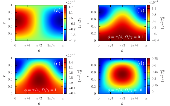
Figure 1: (Color online) Density plot of the dimensionless quantities $1/\gamma{T_{1}}$ [see Eq. (8)] and $1/{\gamma^{2}}{T_{2}^{2}}$ [see Eq. (9)], as a function of the mixing parameter $r\in[0,1]$ and the azimuthal angle $\theta\in[0,\pi]$, respective to the perturbative expansion of the linear entropy for the driven dissipative two-level system around [see Eq. (3)]. In panels (b)–(d), we set the polar angle $\phi=\pi/4$, and consider the ratio $\Omega/\gamma=0.1$ (b), $\Omega/\gamma=1$ (c), and $\Omega/\gamma=0.1$ (d).

Equation (3) is the first main result of the paper. We point out that Eq. (4), which in turn is related to the first-order derivative ${[{f^{(1)}}({\widetilde{\rho}_{t}})]_{t=0}}$ of the purity, has been previously investigated in the context of gain-loss systems Brody and Graefe (2012), the quantum-classical description of non-Hermitian systems Sergi and Giaquinta (2016), and the dynamical instability of pure states Zloshchastiev (2015). In turn, Eq. (III) is related to the second-order time derivative of the purity around $t=0$, and also stands as a main result. The coefficients $|1/{T_{1}}|$ and $|1/{T_{2}}|$ provide timescales for the linear entropy at earlier times of the dynamics, thus predicting the initial growth of the mixedness of the evolved state of the quantum system. Importantly, they can be evaluated once the input state $\rho_{0}$ and the Hamiltonian $H={H_{1}}+i{H_{2}}$ of the system have been specified. Note that $1/T_{1}$ and $1/T_{2}$ depend on the fluctuations of the observable $H_{2}$ that are captured by its covariance respective to the input state. In particular, choosing $H_{2}$ a zero-valued operator, Eqs. (4) and (III) vanish, and one gets that ${S_{L}}({\widetilde{\rho}_{t}})\approx{S_{L}}({\rho_{0}})$. In fact, this is expected since the linear entropy remains invariant for any quantum state undergoing a unitary evolution generated by a Hermitian operator.

In addition, for any initial pure state with ${\rho_{0}^{2}}={\rho_{0}}=|\psi_{0}\rangle\langle{\psi_{0}}|$, and $f({\rho_{0}})=\text{Tr}({\rho_{0}^{2}})=1$, one can verify that Eqs. (4) and (III) imply that $1/{T_{1}}=0$ and $1/{T_{2}^{2}}=0$, regardless of the operators $H_{1}$ and $H_{2}$. In this setting, it can be proved that the mixedness timescales vanish for any perturbative order within the short-time approximation of the linear entropy. Indeed, for the initial pure state $\rho_{0}=|\psi_{0}\rangle\langle{\psi_{0}}|$ undergoing the nonunitary dynamics dictated by the non-Hermitian Hamiltonian $H={H_{1}}+i{H_{2}}$, we have shown in Appendix A that the purity of the state $\widetilde{\rho}_{t}$ is given by $f({\widetilde{\rho}_{t}})=1$, i.e., such state remains pure for all $t\geq 0$. Hence, one gets that the linear entropy identically vanishes, i.e., ${S_{L}}({\widetilde{\rho}_{t}})=[{d}/({d-1})][1-f({\widetilde{\rho}_{t}})]=0$, which implies that any mixedness timescales become zero. Interestingly, we have shown that the same result is obtained within the so-called “metric approach”. Finally, we note that the last term on the right-hand side of Eq. (III) vanishes for $[{H_{1}},{H_{2}}]=0$, i.e., for two commuting operators $H_{1}$ and $H_{2}$.

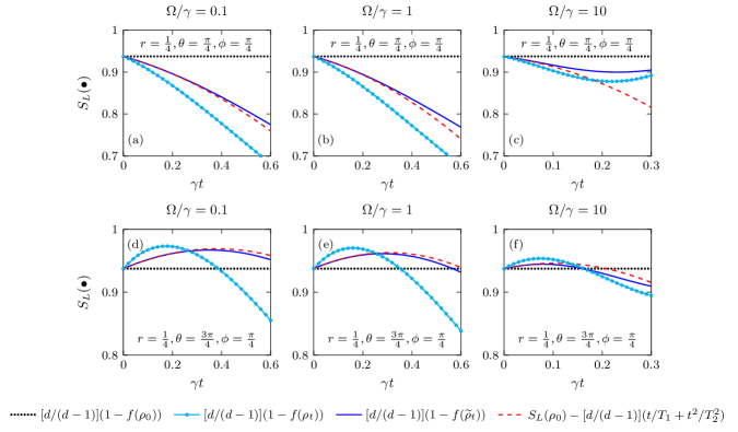
Figure 2: (Color online) Plot of the linear entropy ${S_{L}}({\widetilde{\rho}_{t}})$, as a function of the dimensionless parameter $\gamma t$, for the driven two-level system described by the Hamiltonian $H=\Delta{|1\rangle}{\langle{1}|}+(\Omega/2)(|{0}\rangle\langle{1}|+|{1}\rangle\langle{0}|)$. Here we choose the ratio $\Delta/\gamma=0.5$, and set $\Omega/\gamma=0.1$ (a, d), $\Omega/\gamma=1$ (b, e), and $\Omega/\gamma=10$ (c, f). The system is initialized in the single-qubit state $\rho_{0}=(1/2)(\mathbb{I}+\vec{r}\cdot\vec{\sigma})$, with $\{r,\theta,\phi\}=\{1/4,\pi/4,\pi/4\}$ (a–c), and $\{r,\theta,\phi\}=\{1/4,3\pi/4,\pi/4\}$ (d–f). The black dotted line indicates the linear entropy ${S_{L}}({\rho_{0}})=[d/(d-1)][1-\text{Tr}({\rho_{0}^{2}})]$ respective to the initial state. The cyan dash-dotted line depicts the linear entropy ${S_{L}}({\rho_{t}})=[d/(d-1)][1-\text{Tr}({\rho_{t}^{2}})]$, where $\rho_{t}$ satisfies the Markovian master equation in Eq. (7). The blue solid line indicates the linear entropy ${S_{L}}({\widetilde{\rho}_{t}})=[d/(d-1)][1-\text{Tr}({\widetilde{\rho}_{t}^{2}})]$, where the normalized state ${\widetilde{\rho}_{t}}={\rho_{t}}/\text{Tr}({\rho_{t}})$ fulfills Eq. (2), with ${H_{1}}=H$ and $H_{2}=-(\gamma/2){|1\rangle}{\langle{1}|}$. The red dashed line represents the linear entropy ${S_{L}}({\widetilde{\rho}_{t}})\approx{S_{L}}({\rho_{0}})-[d/(d-1)](t/{T_{1}}+{t^{2}}/{T_{2}^{2}})$ within the short-time approximation [see Eqs. (8) and (9)].

III.1 Example: Dissipative two-level system

To illustrate our findings, we consider a driven two-level system described by the Hamiltonian $H=\Delta{|1\rangle}{\langle{1}|}+(\Omega/2)(|{0}\rangle\langle{1}|+|{1}\rangle\langle{0}|)$, where the two vectors $|0\rangle$ and $|{1}\rangle$ stand for ground and excited states, respectively, with $\Delta$ the energy detuning, and $\Omega$ being their coupling. The system interacts with a zero-temperature thermal reservoir, so that it decays from the excited state $|1\rangle$ to the ground state $|0\rangle$ emitting a photon at a rate $\gamma$. The dynamics is governed by the Markovian master equation

$$\frac{d{\rho_{t}}}{dt}=-i({H_{\text{eff}}}{\rho_{t}}-{\rho_{t}}{H^{\dagger}_{\text{eff}}})+\gamma{L}{\rho_{t}}{L^{\dagger}}~{},$$ (7)

where ${H_{\text{eff}}}=H-i(\gamma/2){L^{\dagger}}{L}$ is the effective non-Hermitian Hamiltonian, while $L=|{0}\rangle\langle{1}|$ is the jump operator Breuer and Petruccione (2002). In the semiclassical regime, i.e., assuming that the effect of quantum jumps is negligible in the time interval under consideration, an effective description of the master equation can be obtained in terms of the coherent nonunitary dissipation of the system, the latter related to the non-Hermitian Hamiltonian ${H_{\text{eff}}}$ Minganti et al. (2019). In this case, by discarding the quantum jump term $\gamma{L}{\rho_{t}}{L^{\dagger}}$, the dynamics of the system is dictated by the equation $d{\rho_{t}}/dt\approx-i({H_{\text{eff}}}{\rho_{t}}-{\rho_{t}}{H^{\dagger}_{\text{eff}}})$, which no longer describes a completely positive and trace-preserving evolution.

To overcome this issue, one introduces the normalized time-dependent density matrix ${\widetilde{\rho}_{t}}={\rho_{t}}/{\text{Tr}({\rho_{t}})}$, which in turn fulfills Eq. (2), with ${H_{1}}=H$ and $H_{2}=-(\gamma/2){|1\rangle}{\langle{1}|}$. The system is initialized in a single-qubit state $\rho_{0}=(1/2)(\mathbb{I}+\vec{r}\cdot\vec{\sigma})$, where $\vec{r}=\{r\sin\theta\cos\phi,r\sin\theta\sin\phi,r\cos\theta\}$ is the Bloch vector, with $r\in[0,1]$, $\theta\in[0,\pi]$ and $\phi\in[0,2\pi[$, while $\vec{\sigma}=\{{\sigma_{x}},{\sigma_{y}},{\sigma_{z}}\}$ is the vector of Pauli matrices, and $\mathbb{I}$ is the $2\times 2$ identity matrix. We will not show the analytical expressions for the exact linear entropy ${S_{L}}({\widetilde{\rho}_{t}})$ of the evolved state as they are cumbersome [see Eq. (1)]. However, it is straightforward to obtain the short-time series expansion of ${S_{L}}({\widetilde{\rho}_{t}})$ applying Eq. (3), with the linear entropy of the input state as ${S_{L}}({\rho_{0}})=1-{r^{2}}$. Using Eqs. (4) and (III), we obtain the following dimensionless coefficients

$$\frac{1}{\gamma\,{T_{1}}}=\frac{1}{2}(1-{r^{2}})\,r\cos\theta~{},$$ (8)

and

$$\frac{1}{{\gamma^{2}}{T_{2}^{2}}}=\frac{1}{8}(1-{r^{2}})\left(1-3{r^{2}}{\cos^{2}}\theta+2\frac{\Omega}{\gamma}\,r\sin\theta\sin\phi\right)~{},$$ (9)

respectively. We see that $1/\gamma{T_{1}}$ is a function of $r$ and $\theta$, while $1/{\gamma^{2}}{T_{2}^{2}}$ depends on the parameters $r$, $\theta$, $\phi$, and $\Omega/\gamma$. We notice that ${S_{L}}({\rho_{0}})$, $1/{T_{1}}$, and $1/{T_{2}}$ approach zero for any initial single-qubit pure state with $r=1$, thus implying that the linear entropy ${S_{L}}({\widetilde{\rho}_{t}})$ is a vanishing quantity in this case.

In Fig. 1 we show the plots of the dimensionless quantities $1/\gamma{T_{1}}$ and $1/{\gamma^{2}}{T_{2}^{2}}$, as a function of the mixing parameter $r$ and the azimuthal angle $\theta$. In Fig. 1(a), we see that $1/\gamma{T_{1}}>0$ for $\theta\in[0,\pi/2)$ and $0<r<1$, while $1/\gamma{T_{1}}<0$ for $\theta\in(\pi/2,\pi]$ and $0<r<1$. In addition, it follows that $1/{\gamma}{T_{1}}=0$ for any chosen initial state with $\theta=\pi/2$ [see Eq. (8)]. Next, Figs. 1(b)–1(d) show the plots of $1/{\gamma^{2}}{T_{2}^{2}}$ in Eq. (9), where we consider the cases $\Omega/\gamma=0.1$ [see Fig. 1(b)], $\Omega/\gamma=1$ [see Fig. 1(c)], and $\Omega/\gamma=10$ [see Fig. 1(d)], also fixing the polar angle $\phi=\pi/4$. On the one hand, for input states with either $\theta=0$ or $\theta=\pi$, that are all incoherent states respective to the computational basis $\{|0\rangle,|1\rangle\}$, Eq. (9) reduces to ${1}/{{\gamma^{2}}{T_{2}^{2}}}=(1/8)(1-{r^{2}})(1-3{r^{2}})$, which is positive for $0\leq r\leq 1/\sqrt{3}$ [see Figs. 1(b)–1(d)]. On the other hand, for initial states lying in the equatorial $xy$ plane with $\theta=\pi/2$, one gets that ${1}/{{\gamma^{2}}{T_{2}^{2}}}=(1/8)(1-{r^{2}})[1+2r(\Omega/\gamma)\sin\phi]$, which is positive for $0\leq\phi\leq\pi$ and $0\leq r\leq 1$. We emphasize that the timescales related to the growth of mixedness can be obtained from the absolute values $|1/\gamma{T_{1}}|$ and $|1/{\gamma}{T_{2}}|$.

Figure 2 shows the plots of the linear entropy ${S_{L}}({\widetilde{\rho}_{t}})$, as a function of the dimensionless parameter $\gamma t$, for the aforementioned driven two-level system. The blue solid line refer to the exact linear entropy ${S_{L}}({\widetilde{\rho}_{t}})$ [see Eq. (1)], while the red dashed line depicts the short-time expansion of this quantity in Eq. (3). We set input states with $\{r,\theta,\phi\}=\{1/4,\pi/4,\pi/4\}$ [see Figs. 2(a)–2(c)], and $\{r,\theta,\phi\}=\{1/4,3\pi/4,\pi/4\}$ [see Figs. 2(d)–2(f)]. In addition, for a fixed ratio $\Delta/\gamma=0.5$, we consider the cases $\Omega/\gamma=0.1$ [see Figs. 2(a) and 2(d)], $\Omega/\gamma=1$ [see Figs. 2(b) and 2(e)], and $\Omega/\gamma=10$ [see Figs. 2(c) and 2(f)]. In each panel, the black dotted line indicates the linear entropy ${S_{L}}({\rho_{0}})=[d/(d-1)][1-\text{Tr}({\rho_{0}^{2}})]$ respective to the initial state. We note that the linear entropy remains invariant under unitary evolutions generated by the Hermitian Hamiltonian $H$, i.e., ${S_{L}}({e^{-itH}}{\rho_{0}}{e^{+itH}})={S_{L}}({\rho_{0}})$. The cyan dash-dotted line displays the linear entropy ${S_{L}}({\rho_{t}})=[d/(d-1)][1-\text{Tr}({\rho_{t}^{2}})]$, with $\rho_{t}$ satisfying the Markovian master equation in Eq. (7). The blue solid line indicates the linear entropy ${S_{L}}({\widetilde{\rho}_{t}})=[d/(d-1)][1-\text{Tr}({\widetilde{\rho}_{t}^{2}})]$, where the normalized state ${\widetilde{\rho}_{t}}={\rho_{t}}/\text{Tr}({\rho_{t}})$ fulfills Eq. (2), with ${H_{1}}=H$ and $H_{2}=-(\gamma/2){|1\rangle}{\langle{1}|}$. The red dashed line represents the linear entropy ${S_{L}}({\widetilde{\rho}_{t}})\approx{S_{L}}({\rho_{0}})-[d/(d-1)](t/{T_{1}}+{t^{2}}/{T_{2}^{2}})$ within the short-time approximation, with the timescales $1/{T_{1}}$ and $1/{T_{2}^{2}}$ given in Eqs. (8) and (9), respectively. In Appendix B, we compare the timescales $1/{T_{1}}$, $1/{T_{2}^{2}}$ and the first-order and second-order time derivatives of the linear entropy for (i) the state $\rho_{t}$ satisfying Eq. (7); (ii) and the normalized state $\widetilde{\rho}_{t}$ fulfilling Eq. (2) related to the effective non-Hermitian Hamiltonian.

Overall, Fig. 2 shows that the short-time approximation of ${S_{L}}({\widetilde{\rho}_{t}})$ correctly reproduces its growth at earlier times of the dynamics. We find that, for $0.01\lesssim\gamma t\lesssim 0.1$, the relative error between the exact linear entropy [see Eq. (1)] and its perturbative expansion [see Eqs. (3), (8), and (9)] is of order ${10^{-7}}\lesssim{\epsilon}\lesssim{10^{-4}}$ for $\Omega/\gamma=0.1$ and $\Omega/\gamma=1$, while it ranges as ${10^{-6}}\lesssim{\epsilon}\lesssim{10^{-3}}$ for $\Omega/\gamma=10$. However, for $\gamma t\gtrsim 0.1$, we have that the latter result is loose and fails to capture the changes in the eigenvalues of the state ${\widetilde{\rho}_{t}}$ driven by the non-Hermitian Hamiltonian. We emphasize that one should look to higher orders in its Taylor expansion to accurately predict the mixedness degree of the evolved state for later times.

IV Mixedness timescale for non-Hermitian bipartite systems

In this section, we provide a mixedness timescale for bipartite quantum systems whose dynamics can be effectively described by a non-Hermitian Hamiltonian. In detail, using the linear entropy as a useful measure of mixedness, we investigate its short-time expansion up to the second order in $t$ for certain time-dependent marginal states of the composite system.

We consider a bipartite quantum system with a finite-dimensional Hilbert space ${\mathcal{H}_{A}}\otimes{\mathcal{H}_{B}}$ split into the subsystems ${\mathcal{H}_{A}}$ and ${\mathcal{H}_{B}}$, with ${d_{A,B}}=\text{dim}\,{\mathcal{H}_{A,B}}$. This composite system is initialized in the quantum state ${\rho^{AB}_{0}}$, which in turn can be chosen either a pure or mixed state, entangled or uncorrelated one, from which the mixed marginal states ${\rho^{A,B}_{0}}={\text{Tr}_{B,A}}({\rho^{AB}_{0}})$ can be obtained. The state ${\rho^{AB}_{0}}$ undergoes a nonunitary evolution generated by the time-independent non-Hermitian Hamiltonian $H={H_{1}}+i{H_{2}}$, with ${H_{1}}=({1}/{2})(H+{H^{\dagger}})$ and ${H_{2}}=-({i}/{2})(H-{H^{\dagger}})$ being noncommuting observables acting over ${\mathcal{H}_{A}}\otimes{\mathcal{H}_{B}}$. It is noteworthy that the operators $H_{1}$ and $H_{2}$ play the role of the Hermitian and anti-Hermitian parts of $H$, respectively. In this setting, it can be proved that the effective dynamics of subsystem $\mathcal{H}_{A,B}$ is governed by the equation of motion Dattoli et al. (1990); Sergi and Zloshchastiev (2013); Zloshchastiev (2015)

$$\frac{d}{dt}{\widetilde{\rho}^{A,B}_{t}} =-i\,{\text{Tr}_{B,A}}([{H_{1}},{\widetilde{\rho}^{AB}_{t}}])+{\text{Tr}_{B,A}}(\{{H_{2}},{\widetilde{\rho}^{AB}_{t}}\})$$

$$-2\,{\text{Tr}_{AB}}({\widetilde{\rho}^{AB}_{t}}{H_{2}})\,{\widetilde{\rho}^{A,B}_{t}}~{},$$ (10)

where ${\widetilde{\rho}^{A,B}_{t}}:={\text{Tr}_{B,A}}({\widetilde{\rho}^{AB}_{t}})$ stands for the time-dependent reduced density matrices, while ${\widetilde{\rho}^{AB}_{t}}:={{\rho^{AB}_{t}}}/{{\text{Tr}_{AB}}({\rho^{AB}_{t}})}$ is the normalized state of the whole system.

Without loss of generality, hereafter we will address the dynamics of the marginal state ${\widetilde{\rho}^{A}_{t}}$, and investigate the short-time behavior of its linear entropy

$${S_{L}}({\widetilde{\rho}^{A}_{t}})=\frac{d_{A}}{({d_{A}}-1)}(1-f({\widetilde{\rho}^{A}_{t}}))~{},$$ (11)

where $f({\widetilde{\rho}^{A}_{t}})={\text{Tr}_{A}}[{({\widetilde{\rho}^{A}_{t}})^{2}}]$ is the purity of the aforementioned reduced density matrix. In this case, by performing a Taylor expansion of ${S_{L}}({\widetilde{\rho}^{A}_{t}})$ up to second order in $t$, around $t=0$, one gets

$${S_{L}}({\widetilde{\rho}^{A}_{t}}) \approx{S_{L}}({\rho_{0}^{A}})-\frac{d_{A}}{({d_{A}}-1)}\left(\frac{1}{T_{1,h}}+\frac{1}{T_{1,nh}}\right)t$$

$$-\frac{d_{A}}{({d_{A}}-1)}\left(\frac{1}{T_{2,h}^{2}}+\frac{1}{T_{2,nh}^{2}}\right){t^{2}}+O({t^{3}})~{},$$ (12)

with ${T_{1,h}}$ and ${T_{1,nh}}$ being coefficients related to the first-order derivative of the linear entropy around $t=0$, and defined as

$${T_{1,h}^{-1}}:={2i}\,{\langle{\text{Tr}_{B}}([{\rho^{AB}_{0}},{H_{1}}])\rangle_{A}}~{},$$ (13)

and

$${T_{1,nh}^{-1}}:=2\,{\langle{\text{Tr}_{B}}(\{{\rho^{AB}_{0}},{H_{2}}\})\rangle_{A}}-4\,f({\rho_{0}^{A}}){\langle{H_{2}}\rangle_{AB}}~{},$$ (14)

while ${T_{2,h}}$ and ${T_{2,nh}}$ arise from the second-order derivative of the linear entropy at the vicinity of $t=0$ as follows

$${T_{2,h}^{-2}} :=-{\langle{\text{Tr}_{B}}([[{\rho^{AB}_{0}},{H_{1}}],{H_{1}}])\rangle_{A}}$$

$$-{\text{Tr}_{A}}\left({({\text{Tr}_{B}}([{\rho^{AB}_{0}},{H_{1}}]))^{2}}\right)~{},$$ (15)

and

$${T_{2,nh}^{-2}}:=$$

$${\langle{\text{Tr}_{B}}(\{\{{\rho^{AB}_{0}},{H_{2}}\},{H_{2}}\})\rangle_{A}}+{\text{Tr}_{A}}\left({({\text{Tr}_{B}}(\{{\rho^{AB}_{0}},{H_{2}}\}))^{2}}\right)$$

$$+i{\langle{\text{Tr}_{B}}(\{[{\rho^{AB}_{0}},{H_{1}}],{H_{2}}\})\rangle_{A}}+i{\langle{\text{Tr}_{B}}([\{{\rho^{AB}_{0}},{H_{2}}\},{H_{1}}])\rangle_{A}}$$

$$-8\,{\langle{H_{2}}\rangle_{AB}}\left({\langle{\text{Tr}_{B}}(\{{\rho^{AB}_{0}},{H_{2}}\})\rangle_{A}}+i\,{\langle{\text{Tr}_{B}}([{\rho^{AB}_{0}},{H_{1}}])\rangle_{A}}\right)$$

$$+2f({\rho_{0}^{A}})\left(i\,{\langle[{H_{2}},{H_{1}}]\rangle_{AB}}-2\left({\langle{H_{2}^{2}}\rangle_{AB}}-3\,{\langle{H_{2}}\rangle_{AB}^{2}}\right)\right)$$

$$-2i\,{\text{Tr}_{A}}\left({\text{Tr}_{B}}([{H_{1}},{\rho^{AB}_{0}}])\,{\text{Tr}_{B}}(\{{\rho^{AB}_{0}},{H_{2}}\})\right)~{}.$$ (16)

Here $\langle\bullet\rangle_{\mu}:={\text{Tr}_{\mu}}(\bullet\,{\rho^{\mu}_{0}})$ defines the expectation value at time $t=0$, with $\mu=\{A,B,AB\}$. We note that Eqs. (13), (14), (IV) and (IV) were obtained from the first-order and second-order derivatives of the quantum purity $f({\widetilde{\rho}^{A}_{t}})$ at the vicinity of $t=0$, with ${[{f^{(1)}}({\widetilde{\rho}^{A}_{t}})]_{t=0}}=1/{T_{1,h}}+1/{T_{1,nh}}$ and $(1/2){[{f^{(2)}}({\widetilde{\rho}^{A}_{t}})]_{t=0}}=1/{T_{2,h}^{2}}+1/{T_{2,nh}^{2}}$.

We point out that Eq. (IV) [see also Eqs. (13)–(IV)] is the second main result of the paper. Overall, we see that the coefficients $|{1/{T_{1,h}}}+{1/{T_{1,nh}}}|$ and ${|{1/{T_{2,h}^{2}}}+{1/{T_{2,nh}^{2}}}|}$ represent first-order and second-order timescales in the initial growth of the mixedness dynamics signaled by linear entropy. On the one hand, both the coefficients $T_{1,h}$ and $T_{2,h}$ depend on the initial state of the bipartite system and the Hermitian part ${H_{1}}$ of the non-Hermitian Hamiltonian. On the other hand, the coefficients $1/{T_{1,nh}}$ and $1/{T_{2,nh}}$ depend on the anti-Hermitian part ${H_{2}}$ of the effective non-Hermitian Hamiltonian. In particular, note that the result in Eqs. (14) and (IV) approach zero in the Hermitian limit $H^{\dagger}=H=H_{1}$, i.e., when one sets $H_{2}$ as a zero-valued observable, regardless of the observable $H_{1}$. This means that $1/{T_{1,nh}}$ and $1/{T_{2,nh}}$ assign first-order and second-order nontrivial corrections to the mixedness timescales that are induced by the effective non-Hermitian Hamiltonian.

To gain insights into understanding the results in Eqs. (IV)–(IV), in the following, we investigate two cases of interest in view of the nonunitary dynamics of non-Hermitian Hamiltonians. The first case describes bipartite quantum systems with initial uncorrelated states. The second one addresses a multiparticle system whose non-Hermitian Hamiltonian corresponds to the transverse-field $XY$ model with next-nearest neighbor couplings and a perturbing term given by an all-to-all Ising Hamiltonian with an imaginary exchange coupling.

IV.1 Separable initial pure states

Here we specialize the result in Eq. (IV) to the particular case of uncorrelated initial pure state ${\rho^{AB}_{0}}={\rho^{A}_{0}}\otimes{\rho^{B}_{0}}$, with ${\rho^{A}_{0}}$ and ${\rho^{B}_{0}}$ normalized pure marginal states, i.e., ${\text{Tr}_{\mu}}[{({\rho^{\mu}_{0}})^{2}}]={\text{Tr}_{\mu}}({\rho^{\mu}_{0}})=1$ for all $\mu=\{A,B,AB\}$. We consider the non-Hermitian Hamiltonian $H={H_{1}}+i{H_{2}}$ with ${H_{1}}={\sum_{n}}\,{A_{n}}\otimes{B_{n}}$ and ${H_{2}}={\sum_{n}}\,{C_{n}}\otimes{D_{n}}$, where ${A_{n}},{C_{n}}\in{\mathcal{H}_{A}}$ and ${B_{n}},{D_{n}}\in{\mathcal{H}_{B}}$ represent noncommuting local observables. In this setting, one can prove that both the coefficients $1/{T_{1,h}}=0$ [see Eq. (13)] and $1/{T_{1,nh}}=0$ [see Eq. (14)] identically vanish, and the linear entropy in Eq. (IV) becomes

$${S_{L}}({\widetilde{\rho}^{A}_{t}})\approx-\frac{d_{A}}{({d_{A}}-1)}\left(\frac{1}{T_{2,h}^{2}}+\frac{1}{T_{2,nh}^{2}}\right){t^{2}}+O({t^{3}})~{},$$ (17)

with the following nonzero coefficients

$${T_{2,h}^{-2}} =-2\,{\sum_{k,l}}\left({\langle{A_{k}}{A_{l}}\rangle_{A}}-{\langle{A_{k}}\rangle_{A}}{\langle{A_{l}}\rangle_{A}}\right)$$

$$\times\left({\langle{B_{k}}{B_{l}}\rangle_{B}}-{\langle{B_{k}}\rangle_{B}}{\langle{B_{l}}\rangle_{B}}\right)~{},$$ (18)

and

$${T_{2,nh}^{-2}} =-2\,{\sum_{k,l}}\left({\langle{C_{k}}{C_{l}}\rangle_{A}}-{\langle{C_{k}}\rangle_{A}}{\langle{C_{l}}\rangle_{A}}\right)$$

$$\times\left({\langle{D_{k}}{D_{l}}\rangle_{B}}-{\langle{D_{k}}\rangle_{B}}{\langle{D_{l}}\rangle_{B}}\right)$$

$$+4\,{\sum_{k,l}}\,\text{Im}[\left({\langle{A_{k}}{C_{l}}\rangle_{A}}-{\langle{A_{k}}\rangle_{A}}{\langle{C_{l}}\rangle_{A}}\right)$$

$$\times\left({\langle{B_{k}}{D_{l}}\rangle_{B}}-{\langle{B_{k}}\rangle_{B}}{\langle{D_{l}}\rangle_{B}}\right)]~{}.$$ (19)

Overall, Eq. (17) implies that the linear entropy varies quadratically at earlier times of the dynamics. We see that $1/{T_{2,h}}$ is proportional to the so-called correlated quantum uncertainty of observables ${A_{n}}\in{\mathcal{H}_{A}}$ and ${B_{n}}\in{\mathcal{H}_{B}}$, thus being entirely determined by the expectation values of these operators with respect to the initial marginal states $\rho^{A,B}_{0}$. It is noteworthy that $|1/{T_{2,h}}|$ assigns a universal timescale for two initially pure subsystems to become entangled by means of the coupling with a Hermitian Hamiltonian $H_{1}$ Kim et al. (1996); Yang (2018); Cresswell (2018).

In turn, the coefficient $1/{T_{2,nh}}$ depends on the correlated quantum uncertainty of observables ${C_{n}}\in{\mathcal{H}_{A}}$ and ${D_{n}}\in{\mathcal{H}_{B}}$, and the imaginary part of cross-correlations of the set of local observables. In particular, one verifies that $1/{T_{2,nh}}$ vanishes in the Hermitian limit $H=H^{\dagger}=H_{1}$, i.e., when choosing zero valued observables $C_{n}$ and $D_{n}$. In this case, one finds that Eq. (IV.1) recovers the so-called idempotency defect for composite systems described by Hermitian Hamiltonians Kim et al. (1996), and constitutes a timescale for the entanglement dynamics of subsystems Yang (2018); Cresswell (2018). In this setting, we see that $1/{T_{2,nh}}$ represents a true signature of the non-Hermitian features of $H$ in the mixedness dynamics. Note that, in addition to the coefficient $1/{T_{2,h}}$, the effective non-Hermitian Hamiltonian induces the factor $1/{T_{2,nh}}$ on the entanglement timescale for initially separable pure states.

IV.2 $1$D quantum many-body systems

Figure 3: (Color online) Plot of the linear entropy ${S_{L}}({\widetilde{\rho}^{A}_{t}})$ for the $k$-particle reduced density matrix ${\widetilde{\rho}_{t}^{A}}$, as a function of the dimensionless parameter $Jt$. The nonunitary evolution of subsystem $A$ is governed by Eq. (IV), with $H_{1}$ being the transverse field $XY$ Hamiltonian in Eq. (20), and $H_{2}$ as the all-to-all Ising model in Eq. (21). The system $A+B$ is initialized in the GHZ mixed state ${\rho^{AB}_{0}}=((1-p)/d)\mathbb{I}+p\,|{\text{GHZ}_{N}}\rangle\langle{\text{GHZ}_{N}}|$, where $|{\text{GHZ}_{N}}\rangle=({1}/{\sqrt{2}})(\,{|0\rangle^{\otimes N}}+{|1\rangle^{\otimes N}})$. Here we set $N=8$, $\gamma=0.75$, ${J_{z}}/J=0.5$, and the mixing parameter $p=0.5$. The blue solid line corresponds to the exact expression of linear entropy in Eq. (11), and the red dashed line indicates its the short-time perturbative expansion in Eq. (IV) [see also Eqs. (IV.2), (25), and (IV.2)].

We set the non-Hermitian Hamiltonian $H={H_{1}}+i{H_{2}}$, where ${H_{1}}$ describes the transverse-field $XY$ model with open boundary conditions as Lieb et al. (1961); Barouch et al. (1970); Barouch and McCoy (1971a, b); McCoy et al. (1971)

$${H_{1}}=-J{\sum_{j=1}^{N-1}}\left({\gamma_{+}}{\sigma_{j}^{x}}{\sigma_{j+1}^{x}}+{\gamma_{-}}{\sigma_{j}^{y}}{\sigma_{j+1}^{y}}\right)-h{\sum_{j=1}^{N}}\,{\sigma_{j}^{z}}~{},$$ (20)

where $J$ is the coupling constant, $h$ represents the external magnetic field along the $z$ axis, and $\gamma_{\pm}=(1\pm\gamma)/2$, with $\gamma$ being the anisotropy parameter. For $\gamma=0$ this Hamiltonian reduces to the isotropic $XX$ model, while for $\gamma=\pm 1$ we recover the Ising model. Furthermore, this model exhibits phase transitions at the isotropic line $\gamma=0$ ($|h|\leq 1$), and at the critical magnetic field $|h|=1$. In turn, $H_{2}$ denotes the many-body fully connected quantum Ising model given by

$${H_{2}}=\frac{J_{z}}{N}\,{\sum_{j<l}}\,{\sigma_{j}^{z}}{\sigma_{l}^{z}}~{},$$ (21)

where $J_{z}$ is the coupling strength, $N$ is the number of spins, and $\{\sigma^{x,y,z}_{s}\}_{s=1,\ldots,N}$ are the Pauli matrices.

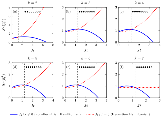
Figure 4: (Color online) Plot of the linear entropy ${S_{L}}({\widetilde{\rho}^{A}_{t}})$ in the short-time approximation [see Eq. (IV)], for the $k$-particle reduced density matrix ${\widetilde{\rho}_{t}^{A}}$, as a function of the dimensionless parameter $Jt$. The nonunitary evolution of subsystem $A$ is governed by Eq. (IV), with $H_{1}$ being the transverse field $XY$ Hamiltonian in Eq. (20), and $H_{2}$ as the all-to-all Ising model in Eq. (21). The system $A+B$ is initialized in the GHZ mixed state ${\rho^{AB}_{0}}=((1-p)/d)\mathbb{I}+p\,|{\text{GHZ}_{N}}\rangle\langle{\text{GHZ}_{N}}|$, where $|{\text{GHZ}_{N}}\rangle=({1}/{\sqrt{2}})(\,{|0\rangle^{\otimes N}}+{|1\rangle^{\otimes N}})$. Here we set $N=8$, $\gamma=0.75$, and the mixing parameter $p=0.5$. The blue solid line corresponds to the case ${J_{z}}/J=0.5$, and the red dashed line depicts the case ${J_{z}}/J=0$.

We consider a bipartition into first sequential $k$ sites ($1,\ldots,k$) as the subsystem $A$, and its complement of sequential $N-k$ sites ($k+1,\ldots,N$) as subsystem $B$. The system $A+B$ is initialized in the mixed state

$${\rho^{AB}_{0}}=\left(\frac{1-p}{d}\right)\mathbb{I}+p\,|{\text{GHZ}_{N}}\rangle\langle{\text{GHZ}_{N}}|~{},$$ (22)

with $d=2^{N}$, $0\leq p\leq 1$, and $|{\text{GHZ}_{N}}\rangle$ is the GHZ state of $N$ particles defined as

$$|{\text{GHZ}_{N}}\rangle=\frac{1}{\sqrt{2}}\left(\,{|0\rangle^{\otimes N}}+{|1\rangle^{\otimes N}}\right)~{},$$ (23)

and its purity is written as $f({\rho^{AB}_{0}})=(1/{2^{N}})(1+({2^{N}}-1)\,{p^{2}})$. Furthermore, one can evaluate the averaged values ${\langle{H_{2}}\rangle_{AB}}=({J_{z}}/2){(N-1)p}$ and ${\langle{H_{2}^{2}}\rangle_{AB}}={J_{z}^{2}}[(N-1)/(4N)](2+(N-2)(N+1)p)$ of the observable $H_{2}$ respective to the probe state of system $A+B$. The many-body state ${\rho^{AB}_{0}}$ undergoes a nonunitary evolution generated by the non-Hermitian Hamiltonian $H={H_{1}}+i{H_{2}}$, and the subsystem $A$ is described by the reduced $k$-particle state ${\widetilde{\rho}^{A}_{t}}={\text{Tr}_{N-k}}({\widetilde{\rho}^{AB}_{t}})$ whose dynamics is governed by Eq. (IV). The linear entropy ${S_{L}}({\widetilde{\rho}^{A}_{t}})$ of this marginal state is given in Eq. (11), which in turn reduces to ${S_{L}}({\rho_{0}^{A}})=[{d_{A}}/({d_{A}}-1)][1-(1/{2^{k}})(1+({2^{k-1}}-1)\,{p^{2}})]$ at time $t=0$. The short-time expansion of ${S_{L}}({\widetilde{\rho}^{A}_{t}})$ is given in Eq. (IV). In this setting, it is possible to verify that the coefficient $1/{T_{1,h}}=0$ vanishes [see Eq. (13)], while Eq. (14) implies the following nonzero contribution

$${T^{-1}_{1,nh}}=$$

$$-\frac{{J_{z}}\,p(1-p)}{{2^{k-1}}N}\left(k(k-1)+N(N-1)({2^{k-1}}-1)p\right)~{}.$$ (24)

It is noteworthy that Eq. (IV.2) shows that $1/{T_{1,nh}}$ exhibits a polynomial dependence on the mixing parameter $p$, thus being a negative quantity for all $0<p<1$, and $k\in\{1,\ldots,N\}$. In particular, it follows that $1/{T_{1,nh}}=0$ for the initial pure state $|{\text{GHZ}_{N}}\rangle\langle{\text{GHZ}_{N}}|$ ($p=1$) and also for the maximally mixed state $\mathbb{I}/d$ ($p=0$). We find that $1/{T_{1,nh}}$ is proportional to the coupling strength $J_{z}$, and identically vanishes in the Hermitian limit (${J_{z}}/J=0$).

Next, by using Eq. (IV), we obtain

$${T^{-2}_{2,h}}=({\delta_{{d_{B}},2}}-1){\gamma^{2}}{J^{2}}{p^{2}}~{},$$ (25)

which depends on the coupling $J$, anisotropy parameter $\gamma$, and vanishes whenever $\mathcal{H}_{B}$ is a two-dimensional subspace, i.e., one gets $1/{T_{2,h}}=0$ for the case ${d_{B}}=2$. Finally, by applying Eq. (IV) and performing lengthy calculations, one obtains the result

$${T^{-2}_{2,nh}}=-\frac{{J_{z}^{2}}}{{2^{k-1}}\,{N^{2}}}\left\{3{N^{2}}{(N-1)^{2}}(1-{2^{k-1}})\,{p^{4}}\right.$$

$$\left.+N(N-1)[({2^{k-1}}-1)(5N(N-1)-2)-4k(k-1)]\,{p^{3}}\right.$$

$$\left.+[k({k^{2}}(k-6)+k+4)+2{N}{k}(k-1)(3N-1)\right.$$

$$\left.-2{N}({2^{k-1}}-1)({N^{3}}-2{N^{2}}+1)]\,{p^{2}}-2k(k-1)\right.$$

$$\left.-k(k-1)[k(k-5)+2((N-1)(N+2)-1)]\,{p}\right\}~{}.$$ (26)

We find that $1/{T^{2}_{2,nh}}$ behaves polynomially with the mixing parameter $p$. In particular, it follows that $1/{T^{2}_{2,nh}}=0$ for $p=1$, while for $p=0$ one obtains that $1/{T^{2}_{2,nh}}={2^{2-k}}{J_{z}^{2}}k(k-1)/{N^{2}}$. Hence, for $N\gg k$, the latter case implies $1/{T^{2}_{2,nh}}\sim{J_{z}^{2}}/{N^{2}}$ for the initial maximally mixed state ($p=0$), i.e, it scales with the inverse square of the number of particles.

Figure 5: (Color online) Plot of the linear entropy ${S_{L}}({\widetilde{\rho}^{A}_{t}})$ [see Eq. (11)] in the short-time approximation [see Eq. (IV)], for the $k$-particle reduced density matrix ${\widetilde{\rho}_{t}^{A}}$, as a function of the dimensionless parameter $Jt$. The nonunitary evolution of subsystem $A$ is governed by Eq. (IV), with $H_{1}$ being the transverse field $XY$ Hamiltonian in Eq. (20), and $H_{2}$ as the all-to-all Ising model in Eq. (21). The system $A+B$ is initialized in the GHZ mixed state ${\rho^{AB}_{0}}=((1-p)/d)\mathbb{I}+p\,|{\text{GHZ}_{N}}\rangle\langle{\text{GHZ}_{N}}|$, where $|{\text{GHZ}_{N}}\rangle=({1}/{\sqrt{2}})(\,{|0\rangle^{\otimes N}}+{|1\rangle^{\otimes N}})$. Here we consider the system size $N=8$, with $k=5$, and $\gamma=0.75$. The blue solid line corresponds to the case ${J_{z}}/J=0.5$, and the red dashed line depicts the case ${J_{z}}/J=0$.

In the following, we will numerically address the short-time dynamics of the linear entropy ${S_{L}}({\widetilde{\rho}^{A}_{t}})$ in Eq. (IV). The system $A+B$ is initialized at the GHZ mixed state in Eq. (22), with $H_{1}$ being the transverse field $XY$ Hamiltonian in Eq. (20), and $H_{2}$ standing for the all-to-all Ising model in Eq. (21). In this case, bearing in mind that $1/{T_{1,h}}=0$, we also apply the results in Eqs. (IV.2), (25), (IV.2). Unless otherwise stated, we set the system size $N=8$, the anisotropy parameter $\gamma=0.75$, and the ratio ${J_{z}}/J=0.5$.

In Fig. 3 we plot of the linear entropy ${S_{L}}({\widetilde{\rho}^{A}_{t}})$, as a function of the dimensionless parameter $Jt$, and set the mixing parameter $p=0.5$. The solid blue line refers to the exact linear entropy ${S_{L}}({\widetilde{\rho}^{A}_{t}})$ [see Eq. (11)], while the red dashed line depicts the short-time expansion of this quantity in Eq. (IV). We consider the subsystem $A$ with the number of sites $k\in\{2,\ldots,7\}$, and respective dimensions ${d_{A}}=\{{2^{k}}\}_{k=2,\ldots,7}$. Figures 3(a)-3(f) show that the short-time expansion of ${S_{L}}({\widetilde{\rho}^{A}_{t}})$ reproduces its growth at early times. In each panel, we find that the relative error between the exact linear entropy [see Eq. (11)] and its respective perturbative expansion [see Eqs. (IV), (IV.2), (25), and (IV.2)] is of order ${10^{-6}}\lesssim{\epsilon}\lesssim{10^{-3}}$ for $0.01\lesssim Jt\lesssim 0.1$. Nevertheless, for $Jt\gtrsim 0.1$, we have that the result in Eq. (IV) becomes loose and it is bounded from above by the exact linear entropy in Eq. (11), thus failing to predict the dynamics of ${S_{L}}({\widetilde{\rho}^{A}_{t}})$ at later times.

Next, Fig. 4 shows the short-time dynamics of the linear entropy ${S_{L}}({\widetilde{\rho}^{A}_{t}})$ in Eq. (IV), for the initial state $\rho_{0}^{AB}$ with $p=0.5$ [see Eq. (22)]. The blue solid line corresponds to the case ${J_{z}}/J=0.5$ (non-Hermitian Hamiltonian), while the red dashed line depicts the case ${J_{z}}/J=0$ (Hermitian Hamiltonian). Overall, Figs. 4(a)–4(e) show that the linear entropy is a concave function for ${J_{z}}/J\neq 0$, while it is a convex function for ${J_{z}}/J=0$. In turn, Fig. 4(f) shows that ${S_{L}}({\widetilde{\rho}^{A}_{t}})$ stands as a concave function for ${J_{z}}/J\neq 0$, while for ${J_{z}}/J=0$ it saturates to a fixed value for all $Jt>0$. To see this, we first note that $1/{T_{1,nh}}=0$ and $1/{T_{2,nh}}=0$ for ${J_{z}}=0$ [see Eqs. (IV.2) and (IV.2), respectively], while one readily obtains that $1/{T_{2,h}}=0$ as the subsystem $B$ has dimension $d_{B}=2$ [see Eq. (25)]. Hence, bearing in mind that $1/{T_{1,h}}=0$, it follows that the linear entropy ${S_{L}}({\widetilde{\rho}^{A}_{t}})\approx{S_{L}}({\rho^{A}_{0}})$ is time-independent in the short-time approximation, for ${J_{z}}/J=0$.

In Fig. 5 we display the short-time dynamics of the linear entropy ${S_{L}}({\widetilde{\rho}^{A}_{t}})$ in Eq. (IV), as a function of $Jt$, and consider the subsystem $A$ with $k=5$ sites. We emphasize that each of the blue solid line corresponds to the case ${J_{z}}/J=0.5$ (non-Hermitian Hamiltonian), and the red ones represent the case ${J_{z}}/J=0$ (Hermitian Hamiltonian). We set the mixing parameters $p=0.25$ [see Fig. 5(a)], $p=0.5$ [see Fig. 5(b)], $p=0.75$ [see Fig. 5(c)], and $p=1$ [see Fig. 5(d)]. In Figs. 5(a) and 5(b), one finds that the linear entropy is concave whenever ${J_{z}}/J\neq 0$, while it turns into a convex function in the Hermitian limit with ${J_{z}}/J=0$. In Fig. 5(c), the linear entropy turn to be a convex function, which is due to the fact that $1/{T_{2,h}}+1/{T_{2,nh}}<0$ for $p=0.75$. Figure 5(d) shows that, for $p=1$, the two linear entropies coincide regardless of the generator $H$. Indeed, we have seen from Eqs. (IV.2) and (IV.2) that $1/{T_{1,nh}}=0$ and $1/{T_{2,nh}}=0$ for initial pure states, respectively. In this case, given that $1/{T_{1,h}}=0$ and ${d_{B}}=8$, the onset growth of the linear entropy satisfies ${S_{L}}({\widetilde{\rho}^{A}_{t}})\approx(16/31)(1+2{\gamma^{2}}{J^{2}}{t^{2}})+O({t^{3}})$ [see Eqs. (IV) and (25)].

As a final remark, Figs. 4 and 5 show that the non-Hermitian Hamiltonian (${J_{z}}/J\neq 0$) enhances the short-time dynamics of ${S_{L}}({\widetilde{\rho}^{A}_{t}})$, which bounds from above the respective linear entropy for the Hermitian Hamiltonian (${J_{z}}/J=0$). Last, Figs. 4 and 5 show a crossover behavior between both the non-Hermitian (${J_{z}}/J\neq 0$) and Hermitian (${J_{z}}/J=0$) cases, but it should be noted that it occurs in a time window that extrapolates the validity of the short-time approximation. Indeed, Fig. 3 shows that our results find good agreement with the numerical simulation of ${S_{L}}({\widetilde{\rho}^{A}_{t}})$ in Eq. (11) for $0\leq Jt\lesssim 0.1$.

V Discussion and Conclusions

In this paper, we discuss the timescales related to the onset growth of linear entropy for finite-dimensional quantum systems described by effective non-Hermitian Hamiltonians. We investigate the short-time perturbative expansion of the linear entropy for a given input state driven by a general non-Hermitian Hamiltonian. We emphasize that our approach takes in account initial quantum states that can be either pure or mixed, possibly entangled or even uncorrelated states. Importantly, for bipartite quantum systems initialized in pure and uncorrelated states, our findings recover the results in Refs. Kim et al. (1996); Yang (2018) to the case of nonunitary reduced dynamics driven by Hermitian Hamiltonians.

We address the degree of mixedness of a quantum state that undergoes the nonunitary dynamics generated by an effective non-Hermitian Hamiltonian $H={H_{1}}+i{H_{2}}$ [see Sec. III]. In this setting, Eq. (3) stands for the short-time expansion of the linear entropy up to second order in time $t$, around $t=0$, which in turn depends on the coefficients $1/{T_{1}}$ and $1/{T_{2}}$ in Eqs. (4) and (III), respectively. Both quantities can be evaluated once the input state and the Hamiltonian $H$ have been specified. We emphasize that Eqs. (4) and (III) provide two competing timescales in the initial growth of the mixedness of the evolved state at earlier times of the dynamics. In particular, both coefficients vanish whenever the system is initialized in a pure state, regardless of the non-Hermitian part of the Hamiltonian. Moreover, in the Hermitian limit, we have that $1/{T_{1}}=0$ and $1/{T_{2}}=0$ independently of the initial state of the system. We note that, since the linear entropy defines a conserved quantity for Hermitian quantum systems, it can be proved that any of the coefficients in its perturbative expansion must vanish in this limiting case [see Eq. (3)].

We specialize these results to the case of a dissipative non-Hermitian two-level system initialized in a mixed single-qubit state [see Sec. III.1]. We find analytical expressions for the coefficients $1/T_{1}$ [see Eq. (8)] and $1/T_{2}$ [see Eq. (9)] in terms of the Bloch sphere parameters. In this case, we compare the exact linear entropy ${S_{L}}({\rho_{t}})$ with its aforementioned short-time expansion around $t=0$. We find good quantitative agreement between these two quantities at earlier times of the dynamics. Of course, for later times one should include higher orders in the Taylor expansion to obtain tighter results for the mixedness of the evolved state.

Next, we investigate the reduced dynamics of composite systems described by non-Hermitian Hamiltonians [see Sec. IV]. We derived the short-time perturbative expansion of the linear entropy ${S_{L}}({\widetilde{\rho}^{A}_{t}})$ for a given time-dependent marginal state of a bipartite system [see Eq. (IV)]. We found that, up to the second order in time $t$, the growth of the linear entropy is governed by the coefficients $1/{T_{1,h}}$ and $1/{T_{1,nh}}$ in Eqs. (13) and (14), respectively, and also $1/{T_{2,h}}$ and $1/{T_{2,nh}}$ in Eqs. (IV) and (IV), respectively. On the one hand, one gets that $1/{T_{1,h}}$ and $1/{T_{2,h}}$ depend on $H_{1}$ and the input state of the system. On the other hand, we have that $1/{T_{1,nh}}$ and $1/{T_{2,nh}}$ depend on $H_{2}$, thus being intrinsically related to the non-Hermitian features of the Hamiltonian. In the Hermitian limit, i.e., when one sets $H_{2}$ being a zero-valued operator, we find $1/{T_{1,nh}}=0$ and $1/{T_{2,nh}}=0$ for any bipartite system.

In particular, specifying an initial pure and uncorrelated state, we find the vanishing coefficients $1/{T_{1,h}}=0$ and $1/{T_{1,nh}}=0$, and the lowest order of the short-time perturbative expansion of the linear entropy ${S_{L}}({\widetilde{\rho}^{A}_{t}})$ depends on $1/{T_{2,h}^{2}}$ and $1/{T_{2,nh}^{2}}$ that are given in Eqs. (IV.1) and (IV.1), respectively [see Sec. IV.1]. In the Hermitian limit, $1/{T_{2,nh}^{2}}$ identically vanishes, and $1/{T_{2,h}^{2}}$ recovers the perturbative expansion of the idempotency defect measuring the coherence losses for composite systems described by Hermitian Hamiltonians Kim et al. (1996). In this setting, we see that $|1/{T_{2,h}}|$ signals the entanglement timescale for quantum systems described by Hermitian Hamiltonians Yang (2018). It is noteworthy that this result is also related to the timescale that governs the growth of entanglement for Rényi entropies Cresswell (2018).

To illustrate these findings, we investigated the linear entropy of the $k$-particle evolved marginal state for a quantum many-body system described by the transverse-field $XY$ model coupled to the imaginary fully connected Ising Hamiltonian [see Sec. IV.2]. We found analytical expressions for $1/{T_{1,nh}}$ and $1/{T_{2,nh}^{2}}$, which in turn scale linearly with the coupling strength of the all-to-all Ising Hamiltonian [see Eqs. (IV.2) and (IV.2), respectively]. In addition, it follows that $1/{T_{1,h}}$ vanishes, while $1/{T_{2,h}^{2}}$ depends on the anisotropy parameter of the $XY$ model [see Eq. (25)]. We compared the short-time expansion of the linear entropy with its exact numerical simulation [see Fig. 3], and discussed its dynamical behavior in both cases of non-Hermitian and Hermitian Hamiltonians [see Figs. 4 and 5]. We find that non-Hermiticity enhances the short-time dynamics of the linear entropy, providing an upper bound for the respective linear entropy for Hermitian Hamiltonian.

Our findings provide insightful qualitative and quantitative information about the initial growth of linear entropy at early times. Importantly, the results require low computational cost and their evaluation involves minimal ingredients as the initial state and the non-Hermitian Hamiltonian that governs the nonunitary dynamics. This might be of interest for higher dimensional systems, where evaluating the linear entropy would require the full spectral decomposition of the evolved system. We point out that one could generalize the present discussion in terms of $\alpha$-Rényi entropies Cresswell (2018). Furthermore, one can investigate the interplay of the aforementioned timescales and the quantum speed limit for nonunitary evolutions generated by non-Hermitian Hamiltonians Pires (2022); Pires and de Oliveira (2021). We hope to address these questions in further investigations. The results in this paper could find applications in the subjects of non-Hermitian quantum sensing Lau and Clerk (2018); Bao et al. (2021), quantum thermodynamics of non-Hermitian systems Gardas et al. (2016), non-Hermitian long-range interacting quantum systems Defenu et al. (2021), and $\mathcal{PT}$-symmetric quantum field theory Bender (2020).

Appendix

A Mixedness for the nonunitary dynamics of initial pure states

In this Appendix, we discuss the mixedness timescales for a given initial pure state whose dynamics is governed by an effective non-Hermitian Hamiltonian. Let us consider a finite-dimensional quantum system initialized in the pure state $\rho_{0}=|{\psi_{0}}\rangle\langle{\psi_{0}}|$, with $\langle{\psi_{0}}|{\psi_{0}}\rangle=1$. In turn, the initial pure state undergoes the nonunitary dynamics generated by a time-independent non-Hermitian Hamiltonian $H={H_{1}}+i{H_{2}}$, with ${H_{1}^{\dagger}}={H_{1}}$ and ${H_{2}^{\dagger}}={H_{2}}$ being Hermitian operators. In this case, the time-dependent normalized density matrix of the system read as

$${\widetilde{\rho}_{t}}=\frac{{U_{t}}{\rho_{0}}{U_{t}^{\dagger}}}{\text{Tr}({U_{t}}{\rho_{0}}{U_{t}^{\dagger}})}=\frac{{U_{t}}|{\psi_{0}}\rangle\langle{\psi_{0}}|{U_{t}^{\dagger}}}{\langle{\psi_{0}}|{U_{t}^{\dagger}}{U_{t}}|{\psi_{0}}\rangle}~{},$$ (A1)

with ${U_{t}}={e^{-itH}}$ being the nonunitary evolution operator. It can be proved that the normalized state ${\widetilde{\rho}_{t}}$ in Eq. (A1) fulfills the differential equation ${d{\widetilde{\rho}_{t}}}/{dt}=-i[{H_{1}},{\widetilde{\rho}_{t}}]+\{{H_{2}},{\widetilde{\rho}_{t}}\}-2\text{Tr}({\widetilde{\rho}_{t}}{H_{2}})\,{\widetilde{\rho}_{t}}$, which in turn describes a completely positive and trace preserving evolution. In this case, the purity $f({\widetilde{\rho}_{t}})=\text{Tr}({\widetilde{\rho}_{t}^{2}})$ of the evolved state thus yields

$$f({\widetilde{\rho}_{t}})=\frac{\text{Tr}({U_{t}}|{\psi_{0}}\rangle\langle{\psi_{0}}|{U_{t}^{\dagger}}{U_{t}}|{\psi_{0}}\rangle\langle{\psi_{0}}|{U_{t}^{\dagger}})}{\langle{\psi_{0}}|{U_{t}^{\dagger}}{U_{t}}|{\psi_{0}}\rangle^{2}}=1~{},$$ (A2)

where we have used the cyclic property of the trace. Equation (A2) shows that, for an initial pure state $\rho_{0}=|{\psi_{0}}\rangle\langle{\psi_{0}}|$, the purity of the evolved normalized state $\widetilde{\rho}_{t}$ will remain constant, i.e., such state remains pure for all $t\geq 0$. The linear entropy identically vanishes, i.e., ${S_{L}}({\widetilde{\rho}_{t}})=[{d}/({d-1})][1-f({\widetilde{\rho}_{t}})]=0$. Hence, for all nonzero positive integer $k\in\mathbb{Z}^{+}$, the $k$th-order time derivative of both the purity and linear entropy will vanish, i.e., one gets ${d^{k}}{f}({\widetilde{\rho}_{t}})/d{t^{k}}=0$ and ${d^{k}}{S_{L}}({\widetilde{\rho}_{t}})/d{t^{k}}=0$. This result proves that, given an initial pure state undergoing the nonunitary dynamics generated by a non-Hermitian Hamiltonian, the mixedness timescales vanish for any perturbative order within the short-time approximation of the linear entropy. See also Refs. Brody and Graefe (2012); Sergi and Zloshchastiev (2016); Sergi and Giaquinta (2016); Sergi and Zloshchastiev (2013); Zloshchastiev (2015).

Next, we show that the same result can obtained when considering the so-called “metric approach” for non-Hermitian systems, whose main idea relies on modifying the inner-product structure of the Hilbert space Bender (2007); Mostafazadeh (2010). Indeed, the Hilbert space is endowed with an inner-product related to the time-dependent operator $G_{t}$ called “metric” Brody (2013). Let $H\neq H^{\dagger}$ be the effective time-independent non-Hermitian Hamiltonian governing the nonunitary dynamics of a finite-dimensional quantum system. In this setting, given the initial pure state $\rho_{0}=|{\psi_{0}}\rangle\langle{\psi_{0}}|$, one gets that the evolved state $|{\psi_{t}}\rangle={U_{t}}|{\psi_{0}}\rangle={e^{-itH}}|{\psi_{0}}\rangle$ is not properly normalized, i.e., its squared norm $\langle{\psi_{t}}|{\psi_{t}}\rangle=\langle{\psi_{0}}|{U_{t}}{U_{t}^{\dagger}}|{\psi_{0}}\rangle$ stands as a time-dependent quantity (${U_{t}^{\dagger}}\neq{U_{t}^{-1}}$). To overcome this issue, one introduces the modified dual vector $({\psi_{t}}|:=\langle{\psi_{t}}|{G_{t}}$ that is obtained replacing the conventional Hermitian conjugate, where $G_{t}$ is a time-dependent, Hermitian, and positive definite operator called metric Brody (2013). In this approach, the inner product $({\psi_{t}}|{\psi_{t}}\rangle$ is required to be time-independent, i.e., its time derivative is expected to vanish as $d({\psi_{t}}|{\psi_{t}}\rangle/dt=d\langle{\psi_{t}}|{G_{t}}|{\psi_{t}}\rangle/dt=0$, for all $t\geq 0$. In turn, this constraint implies that the metric operator $G_{t}$ fulfills the differential equation

$$\frac{d{G_{t}}}{dt}=i({G_{t}}H-{H^{\dagger}}{G_{t}})~{}.$$ (A3)

We point out that, even though $|{\psi_{t}\rangle}$ exhibits a time-independent squared norm, the vector $|{\psi_{t}\rangle}$ is no longer normalized to the unity. This motivates to recast the evolved dual state as ${({\psi_{t}}|{\psi_{t}}\rangle^{-1}}({\psi_{t}}|$, and thus the time-dependent density matrix of the system yields

$${\rho_{t}}=\frac{|{\psi_{t}}\rangle({\psi_{t}}|}{({\psi_{t}}|{\psi_{t}}\rangle}=\frac{|{\psi_{t}}\rangle\langle{\psi_{t}}|{G_{t}}}{\langle{\psi_{t}}|{G_{t}}|{\psi_{t}}\rangle}~{}.$$ (A4)

In this setting, it can be seen that the purity $f({\rho_{t}})=\text{Tr}({\rho_{t}^{2}})$ of the evolved state will remain constant and equal to the unity for all $t\geq 0$,

$$f({\rho_{t}})=\frac{\text{Tr}(|{\psi_{t}}\rangle\langle{\psi_{t}}|{G_{t}}|{\psi_{t}}\rangle\langle{\psi_{t}}|{G_{t}})}{\langle{\psi_{t}}|{G_{t}}|{\psi_{t}}\rangle^{2}}=1~{},$$ (A5)

where we have applied the cyclic property of the trace. Equation (A5) implies that, for any initial pure state, the linear entropy of the evolved state becomes zero, i.e., ${S_{L}}({\rho_{t}})=[{d}/({d-1})][1-f({\rho_{t}})]=0$, for all $t\geq 0$. Therefore, given an initial pure state, Eqs. (A2) and (A5) show that the purity of its evolved state must be the same regardless of the theoretical framework that was applied to address the nonunitary dynamics generated by a non-Hermitian Hamiltonian.

B Timescales for the dissipative two-level system

In this Appendix, we compare the timescales $1/(\gamma{T_{1}})$ [see Eq. (8)] and $1/({\gamma^{2}}{T_{2}^{2}})$ [see Eq. (9)] with both the first-order $-[d{S_{L}}(\bullet)/dt]_{t=0}$ and second-order $-[{d^{2}}{S_{L}}(\bullet)/d{t^{2}}]_{t=0}$ time derivatives around $t=0$ of the linear entropy, for the dissipative two-level system discussed in Sec. III.1. We remind that the system is described by the Hamiltonian $H=\Delta{|1\rangle}{\langle{1}|}+(\Omega/2)(|{0}\rangle\langle{1}|+|{1}\rangle\langle{0}|)$, and one sets the probe single-qubit state $\rho_{0}=(1/2)(\mathbb{I}+\vec{r}\cdot\vec{\sigma})$. Hereafter, we choose $\Delta/\gamma=0.5$, and also set $\{\theta,\phi\}=\{3\pi/4,\pi/4\}$. The overall dynamics of the dissipative systems is governed by the Markovian master equation in Eq. (7). It is noteworthy that by neglecting the effect of quantum jumps, the nonunitary dynamics of the system is recast in terms of the effective non-Hermitian Hamiltonian ${H_{\text{eff}}}={H_{1}}+i{H_{2}}$, with $H_{1}=H$ and ${H_{2}}=-(\gamma/2){|1\rangle}{\langle{1}|}$.

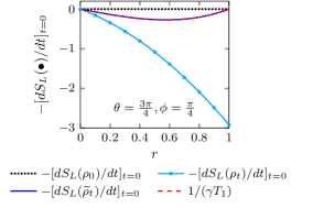
Figure 6: (Color online) Plot of the first-order time derivative $-[d{S_{L}}(\bullet)/dt]_{t=0}$ around $t=0$ of the linear entropy, and the timescale $1/\gamma{T_{1}}$, as a function of the Bloch sphere radius $r$, for the driven two-level system described by the Hamiltonian $H=\Delta{|1\rangle}{\langle{1}|}+(\Omega/2)(|{0}\rangle\langle{1}|+|{1}\rangle\langle{0}|)$. Here we choose the ratio $\Delta/\gamma=0.5$, and $\Omega/\gamma=0.1$. The system is initialized in the single-qubit state $\rho_{0}=(1/2)(\mathbb{I}+\vec{r}\cdot\vec{\sigma})$, with $\{\theta,\phi\}=\{3\pi/4,\pi/4\}$. The black dotted line indicates $-[d{S_{L}}({\rho_{0}})/dt]_{t=0}$, with ${S_{L}}({e^{-itH}}{\rho_{0}}{e^{+itH}})={S_{L}}(\rho_{0})$. The cyan dash-dotted line depicts the quantity $-[d{S_{L}}({\rho_{t}})/dt]_{t=0}$, with the state $\rho_{t}$ evolving under the Markovian master equation in Eq. (7). The blue solid line indicates the first-order time-derivative $-[d{S_{L}}({\widetilde{\rho}_{t}})/dt]_{t=0}$, with the normalized state ${\widetilde{\rho}_{t}}={\rho_{t}}/\text{Tr}({\rho_{t}})$ satisfying Eq. (2), where ${H_{1}}=H$ and $H_{2}=-(\gamma/2){|1\rangle}{\langle{1}|}$. The red dashed line displays the timescale $1/(\gamma{T_{1}})$ [see Eq. (8)].

In Fig. 6, we show plots of $-[d{S_{L}}(\bullet)/dt]_{t=0}$ and $1/(\gamma{T_{1}})$, as a function of the Bloch sphere radius $r$. We set $\Omega/\gamma=0.1$, but we find that the plots are not sensitive to changes in the ratio $\Omega/\gamma$ [see also Fig. 1(a)]. The black dotted line indicates the first-order time derivative $-{[d{S_{L}}({\rho_{0}})/dt]_{t=0}}$. Note that this quantity is equal to zero, since the linear entropy ${S_{L}}({e^{-itH}}{\rho_{0}}{e^{+itH}})={S_{L}}(\rho_{0})$ is time-independent for a unitary evolution generated by the Hermitian Hamiltonian $H$. The cyan dash-dotted line displays the first-order time derivative $-[d{S_{L}}({\rho_{t}})/dt]_{t=0}$, where $\rho_{t}$ satisfies the Markovian master equation in Eq. (7). The blue solid line depicts the quantity $-[d{S_{L}}({\widetilde{\rho}_{t}})/dt]_{t=0}$, where ${\widetilde{\rho}_{t}}$ satisfies Eq. (2). The dashed red line displays the timescale $1/(\gamma{T_{1}})$ in Eq. (8). The quantities $-[d{S_{L}}({\widetilde{\rho}_{t}})/dt]_{t=0}$ and $1/(\gamma{T_{1}})$ coincide each other.

In Fig. 7, we show plots of $-(1/2)[{d^{2}}{S_{L}}(\bullet)/d{t^{2}}]_{t=0}$ and $1/({\gamma^{2}}{T_{2}^{2}})$, as a function of the Bloch sphere radius $r$. We set $\Omega/\gamma=0.1$ [see Fig. 7(a)], $\Omega/\gamma=1$ [see Fig. 7(b)], and $\Omega/\gamma=10$ [see Fig. 7(c)]. The black dotted line indicates the quantity $-[{d^{2}}{S_{L}}({\rho_{0}})/d{t^{2}}]_{t=0}$, which in turn vanishes for the probe state undergoing the unitary evolution generated by $H$. The cyan dash-dotted line shows the quantity $-(1/2)[{d^{2}}{S_{L}}({\rho_{t}})/d{t^{2}}]_{t=0}$, with $\rho_{t}$ satisfying Eq. (7). The blue solid line displays the second-order time derivative $-(1/2)[{d^{2}}{S_{L}}({\widetilde{\rho}_{t}})/d{t^{2}}]_{t=0}$, where ${\widetilde{\rho}_{t}}$ fulfills Eq. (2). The dashed red line represents the timescale $1/({\gamma^{2}}{T_{2}^{2}})$. Note that the quantities $-[{d^{2}}{S_{L}}({\widetilde{\rho}_{t}})/d{t^{2}}]_{t=0}$ and $1/({\gamma^{2}}{T_{2}^{2}})$ agree with each other.

In the following, we comment on the differences in the plots of Figs. 6 and 7. On the one hand, the quantities $-[d{S_{L}}({\rho_{t}})/dt]_{t=0}$ and $-(1/2)[{d^{2}}{S_{L}}({\rho_{t}})/d{t^{2}}]_{t=0}$ are related to the linear entropy of state $\rho_{t}$ whose dynamics is governed by Eq. (7). On the other hand, note that $-{[d{S_{L}}({\widetilde{\rho}_{t}})/dt]_{t=0}}$ and $-(1/2){[{d^{2}}{S_{L}}({\widetilde{\rho}_{t}})/d{t^{2}}]_{t=0}}$ depend on the linear entropy of the normalized state $\widetilde{\rho}_{t}$ that undergoes the nonunitary effective dynamics generated by the non-Hermitian Hamiltonian ${H_{\text{eff}}}={H_{1}}+i{H_{2}}$, discarding quantum jumps [see Eq. (2)]. As expected, these last two time derivatives agree with the timescales $1/({\gamma}{T_{1}})$ and $1/({\gamma^{2}}{T_{2}^{2}})$, respectively.

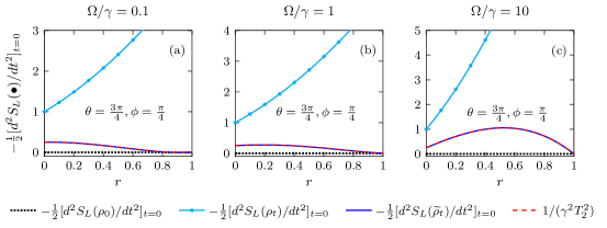
Figure 7: (Color online) Plot of the second-order time derivative $-(1/2)[{d^{2}}{S_{L}}(\bullet)/d{t^{2}}]_{t=0}$ around $t=0$ of the linear entropy, and the timescale $1/{\gamma^{2}}{T_{2}^{2}}$, as a function of the radius $r$ of the Bloch sphere, for the driven two-level system described by the Hamiltonian $H=\Delta{|1\rangle}{\langle{1}|}+(\Omega/2)(|{0}\rangle\langle{1}|+|{1}\rangle\langle{0}|)$. The system is initialized in the single-qubit state $\rho_{0}=(1/2)(\mathbb{I}+\vec{r}\cdot\vec{\sigma})$, with $\{\theta,\phi\}=\{3\pi/4,\pi/4\}$. We set $\Omega/\gamma=0.1$ (a), $\Omega/\gamma=1$ (b), and $\Omega/\gamma=10$ (c). The black dotted line shows the second-order time derivative $-(1/2)[{d^{2}}{S_{L}}({\rho_{0}})/d{t^{2}}]_{t=0}$. The cyan dash-dotted line depicts the quantity $-(1/2)[{d^{2}}{S_{L}}({\rho_{t}})/d{t^{2}}]_{t=0}$, where the state $\rho_{t}$ fulfills Eq. (7). The blue solid line indicates the quantity $-(1/2)[{d^{2}}{S_{L}}({\widetilde{\rho}_{t}})/d{t^{2}}]_{t=0}$, with the normalized state ${\widetilde{\rho}_{t}}={\rho_{t}}/\text{Tr}({\rho_{t}})$ satisfying Eq. (2), where ${H_{1}}=H$ and $H_{2}=-(\gamma/2){|1\rangle}{\langle{1}|}$. The red dashed line displays the timescale $1/({\gamma^{2}}{T_{2}^{2}})$ [see Eq. (9)].

References

- Brody and Graefe (2012) D. C. Brody and E.-M. Graefe, “Mixed-State Evolution in the Presence of Gain and Loss,” Phys. Rev. Lett. 109, 230405 (2012).
- Roccati et al. (2022) F. Roccati, G. M. Palma, F. Ciccarello, and F. Bagarello, “Non-Hermitian Physics and Master Equations,” Open Syst. Inf. Dyn. 29, 2250004 (2022).
- Yu et al. (2020) S. Yu, Y. Meng, J.-S. Tang, X.-Y. Xu, Y.-T. Wang, P. Yin, Z.-J. Ke, W. Liu, Z.-P. Li, Y.-Z. Yang, G. Chen, Y.-J. Han, C.-F. Li, and G.-C. Guo, “Experimental Investigation of Quantum -Enhanced Sensor,” Phys. Rev. Lett. 125, 240506 (2020).
- Wang et al. (2021) K. Wang, L. Xiao, J. C. Budich, W. Yi, and P. Xue, “Simulating Exceptional Non-Hermitian Metals with Single-Photon Interferometry,” Phys. Rev. Lett. 127, 026404 (2021).
- Zyablovsky et al. (2016) A. A. Zyablovsky, E. S. Andrianov, and A. A. Pukhov, “Parametric instability of optical non-Hermitian systems near the exceptional point,” Sci. Rep. 6, 29709 (2016).
- Kawabata et al. (2017) K. Kawabata, Y. Ashida, and M. Ueda, “Information Retrieval and Criticality in Parity-Time-Symmetric Systems,” Phys. Rev. Lett. 119, 190401 (2017).
- Delplace et al. (2021) P. Delplace, T. Yoshida, and Y. Hatsugai, “Symmetry-Protected Multifold Exceptional Points and Their Topological Characterization,” Phys. Rev. Lett. 127, 186602 (2021).
- Ashida et al. (2020) Y. Ashida, Z. Gong, and M. Ueda, “Non-Hermitian physics,” Adv. Phys. 69, 249 (2020).
- Bergholtz et al. (2021) E. J. Bergholtz, J. C. Budich, and F. K. Kunst, “Exceptional topology of non-Hermitian systems,” Rev. Mod. Phys. 93, 015005 (2021).
- Shackleton and Scheurer (2020) H. Shackleton and M. S. Scheurer, “Protection of parity-time symmetry in topological many-body systems: Non-Hermitian toric code and fracton models,” Phys. Rev. Research 2, 033022 (2020).
- Tzeng et al. (2021) Y.-C. Tzeng, C.-Y. Ju, G.-Y. Chen, and W.-M. Huang, “Hunting for the non-Hermitian exceptional points with fidelity susceptibility,” Phys. Rev. Research 3, 013015 (2021).
- Lourenço et al. (2022) J. A. S. Lourenço, G. Higgins, C. Zhang, M. Hennrich, and T. Macrì, “Non-Hermitian dynamics and -symmetry breaking in interacting mesoscopic Rydberg platforms,” Phys. Rev. A 106, 023309 (2022).
- Sticlet et al. (2022) D. Sticlet, B. Dóra, and C. P. Moca, “Kubo Formula for Non-Hermitian Systems and Tachyon Optical Conductivity,” Phys. Rev. Lett. 128, 016802 (2022).
- Korff and Weston (2007) C. Korff and R. Weston, “PT symmetry on the lattice: The quantum group invariant XXZ spin chain,” J. Phys. A: Math. Theor. 40, 8845 (2007).
- Korff (2008) C. Korff, “PT symmetry of the non-Hermitian XX spin-chain: Non-local bulk interaction from complex boundary fields,” J. Phys. A: Math. Theor. 41, 295206 (2008).
- Castro-Alvaredo and Fring (2009) O. A. Castro-Alvaredo and A. Fring, “A spin chain model with non-Hermitian interaction: The Ising quantum spin chain in an imaginary field,” J. Phys. A: Math. Theor. 42, 465211 (2009).
- Ashida et al. (2017) Y. Ashida, S. Furukawa, and M. Ueda, “Parity-time-symmetric quantum critical phenomena,” Nat. Commun. 8, 15791 (2017).
- Xiao et al. (2019) L. Xiao, K. Wang, X. Zhan, Z. Bian, K. Kawabata, M. Ueda, W. Yi, and P. Xue, “Observation of Critical Phenomena in Parity-Time-Symmetric Quantum Dynamics,” Phys. Rev. Lett. 123, 230401 (2019).
- Lee et al. (2020) E. Lee, H. Lee, and B.-J. Yang, “Many-body approach to non-Hermitian physics in fermionic systems,” Phys. Rev. B 101, 121109(R) (2020).
- Hamazaki et al. (2019) R. Hamazaki, K. Kawabata, and M. Ueda, “Non-Hermitian Many-Body Localization,” Phys. Rev. Lett. 123, 090603 (2019).
- Matsumoto et al. (2020) N. Matsumoto, K. Kawabata, Y. Ashida, S. Furukawa, and M. Ueda, “Continuous Phase Transition without Gap Closing in Non-Hermitian Quantum Many-Body Systems,” Phys. Rev. Lett. 125, 260601 (2020).
- Takasu et al. (2020) Y. Takasu, T. Yagami, Y. Ashida, R. Hamazaki, Y. Kuno, and Y. Takahashi, “PT-symmetric non-Hermitian quantum many-body system using ultracold atoms in an optical lattice with controlled dissipation,” Prog. Theor. Exp. Phys. 2020, 12A110 (2020).
- Turkeshi and Schiró (2023) X. Turkeshi and M. Schiró, “Entanglement and correlation spreading in non-Hermitian spin chains,” Phys. Rev. B 107, L020403 (2023).
- Gal et al. (2022) Y. L. Gal, X. Turkeshi, and M. Schiró, “Volume-to-Area Law Entanglement Transition in a non-Hermitian Free Fermionic Chain,” arXiv:2210.11937 (2022).
- Kawabata et al. (2020) K. Kawabata, M. Sato, and K. Shiozaki, “Higher-order non-Hermitian skin effect,” Phys. Rev. B 102, 205118 (2020).
- Peng et al. (2022) Y. Peng, J. Jie, D. Yu, and Y. Wang, “Manipulating the non-Hermitian skin effect via electric fields,” Phys. Rev. B 106, L161402 (2022).
- Žnidarič (2022) M. Žnidarič, “Solvable non-Hermitian skin effect in many-body unitary dynamics,” Phys. Rev. Research 4, 033041 (2022).
- Yao and Wang (2018) S. Yao and Z. Wang, “Edge States and Topological Invariants of Non-Hermitian Systems,” Phys. Rev. Lett. 121, 086803 (2018).
- Yang et al. (2020) Z. Yang, K. Zhang, C. Fang, and J. Hu, “Non-Hermitian Bulk-Boundary Correspondence and Auxiliary Generalized Brillouin Zone Theory,” Phys. Rev. Lett. 125, 226402 (2020).
- Pará et al. (2021) Y. Pará, G. Palumbo, and T. Macrì, “Probing non-hermitian phase transitions in curved space via quench dynamics,” Phys. Rev. B 103, 155417 (2021).
- Nakanishi and Sasamoto (2022) Y. Nakanishi and T. Sasamoto, “ phase transition in open quantum systems with Lindblad dynamics,” Phys. Rev. A 105, 022219 (2022).
- Noronha et al. (2022) F. Noronha, J. A. S. Lourenço, and T. Macrì, “Robust quantum boomerang effect in non-Hermitian systems,” Phys. Rev. B 106, 104310 (2022).
- Sajjad et al. (2022) R. Sajjad, J. L. Tanlimco, H. Mas, A. Cao, E. Nolasco-Martinez, E. Q. Simmons, F. L. N. Santos, P. Vignolo, T. Macrì, and D. M. Weld, “Observation of the Quantum Boomerang Effect,” Phys. Rev. X 12, 011035 (2022).
- Prat et al. (2019) T. Prat, D. Delande, and N. Cherroret, “Quantum boomeranglike effect of wave packets in random media,” Phys. Rev. A 99, 023629 (2019).
- Noronha and Macrì (2022) F. Noronha and T. Macrì, “Ubiquity of the quantum boomerang effect in Hermitian Anderson-localized systems,” Phys. Rev. B 106, L060301 (2022).
- Minganti et al. (2019) F. Minganti, A. Miranowicz, R. W. Chhajlany, and F. Nori, “Quantum exceptional points of non-Hermitian Hamiltonians and Liouvillians: The effects of quantum jumps,” Phys. Rev. A 100, 062131 (2019).
- Minganti et al. (2020) F. Minganti, A. Miranowicz, R. W. Chhajlany, I. I. Arkhipov, and F. Nori, “Hybrid-Liouvillian formalism connecting exceptional points of non-Hermitian Hamiltonians and Liouvillians via postselection of quantum trajectories,” Phys. Rev. A 101, 062112 (2020).
- Pires and Macrì (2021) D. P. Pires and T. Macrì, “Probing phase transitions in non-Hermitian systems with multiple quantum coherences,” Phys. Rev. B 104, 155141 (2021).
- Huang et al. (2021) K.-Q. Huang, W.-L. Zhao, and Z. Li, “Effective protection of quantum coherence by a non-Hermitian driving potential,” Phys. Rev. A 104, 052405 (2021).
- Gopalakrishnan and Gullans (2021) S. Gopalakrishnan and M. J. Gullans, “Entanglement and Purification Transitions in Non-Hermitian Quantum Mechanics,” Phys. Rev. Lett. 126, 170503 (2021).
- Chen et al. (2022a) L.-M. Chen, Y. Zhou, S. A. Chen, and P. Ye, “Quantum entanglement of non-Hermitian quasicrystals,” Phys. Rev. B 105, L121115 (2022a).
- Fang et al. (2022) Y.-L. Fang, J.-L. Zhao, D.-X. Chen, Y.-H. Zhou, Y. Zhang, Q.-C. Wu, C.-P. Yang, and F. Nori, “Entanglement dynamics in anti--symmetric systems,” Phys. Rev. Research 4, 033022 (2022).
- Ortega-Taberner et al. (2022) C. Ortega-Taberner, L. Rødland, and M. Hermanns, “Polarization and entanglement spectrum in non-Hermitian systems,” Phys. Rev. B 105, 075103 (2022).
- Macieszczak et al. (2019) K. Macieszczak, E. Levi, T. Macrì, I. Lesanovsky, and J. P. Garrahan, “Coherence, entanglement, and quantumness in closed and open systems with conserved charge, with an application to many-body localization,” Phys. Rev. A 99, 052354 (2019).
- Pires et al. (2020) D. P. Pires, A. Smerzi, and T. Macrì, “Relating relative Rényi entropies and Wigner-Yanase-Dyson skew information to generalized multiple quantum coherences,” Phys. Rev. A 102, 012429 (2020).
- Sergi and Zloshchastiev (2016) A. Sergi and K. G. Zloshchastiev, “Quantum entropy of systems described by non-Hermitian Hamiltonians,” J. Stat. Mech. 2016, 033102 (2016).
- Zhang et al. (2017) S.-Y. Zhang, M.-F. Fang, and L. Xu, “Quantum entropy of non-Hermitian entangled systems,” Quantum Inf. Process. 16, 234 (2017).
- Guo et al. (2021) Y.-B. Guo, Y.-C. Yu, R.-Z. Huang, L.-P. Yang, R.-Z. Chi, Hai-Jun Liao, and T. Xiang, “Entanglement entropy of non-Hermitian free fermions,” J. Phys.: Condens. Matter 33, 475502 (2021).
- Chen et al. (2022b) W. Chen, L. Peng, H. Lu, and X. Lu, “Characterizing bulk-boundary correspondence of one-dimensional non-Hermitian interacting systems by edge entanglement entropy,” Phys. Rev. B 105, 075126 (2022b).
- Li et al. (2017) J. Li, R. Fan, H. Wang, B. Ye, B. Zeng, H. Zhai, X. Peng, and J. Du, “Measuring Out-of-Time-Order Correlators on a Nuclear Magnetic Resonance Quantum Simulator,” Phys. Rev. X 7, 031011 (2017).
- Streltsov et al. (2018) A. Streltsov, H. Kampermann, S. Wölk, M. Gessner, and D. Bruß, “Maximal coherence and the resource theory of purity,” New J. Phys. 20, 053058 (2018).
- Islam et al. (2015) R. Islam, R. Ma, P. M. Preiss, M. E. Tai, A. Lukin, M. Rispoli, and M. Greiner, “Measuring entanglement entropy in a quantum many-body system,” Nature (London) 528, 77 (2015).
- Elben et al. (2018) A. Elben, B. Vermersch, M. Dalmonte, J. I. Cirac, and P. Zoller, “Rényi Entropies from Random Quenches in Atomic Hubbard and Spin Models,” Phys. Rev. Lett. 120, 050406 (2018).
- Kaufman et al. (2016) A. M. Kaufman, M. E. Tai, A. Lukin, M. Rispoli, R. Schittko, P. M. Preiss, and M. Greiner, “Quantum thermalization through entanglement in an isolated many-body system,” Science 353, 794 (2016).
- Linke et al. (2018) N. M. Linke, S. Johri, C. Figgatt, K. A. Landsman, A. Y. Matsuura, and C. Monroe, “Measuring the Rényi entropy of a two-site Fermi-Hubbard model on a trapped ion quantum computer,” Phys. Rev. A 98, 052334 (2018).
- Brydges et al. (2019) T. Brydges, A. Elben, P. Jurcevic, B. Vermersch, C. Maier, B. P. Lanyon, P. Zoller, R. Blatt, and C. F. Roos, “Probing Rényi entanglement entropy via randomized measurements,” Science 364, 260 (2019).
- Yang (2018) I.-S. Yang, “Entanglement timescale,” Phys. Rev. D 97, 066008 (2018).
- Cresswell (2018) J. C. Cresswell, “Universal entanglement timescale for Rényi entropies,” Phys. Rev. A 97, 022317 (2018).
- Angelo and Furuya (2005) R. M. Angelo and K. Furuya, “Semiclassical limit of the entanglement in closed pure systems,” Phys. Rev. A 71, 042321 (2005).
- Nemes and de Toledo Piza (1986) M. C. Nemes and A. F. R. de Toledo Piza, “Effective dynamics of quantum subsystems,” Phys. A: Stat. Mech. Appl. 137, 367 (1986).
- Zurek (2003) W. H. Zurek, “Decoherence, einselection, and the quantum origins of the classical,” Rev. Mod. Phys. 75, 715 (2003).
- Kim et al. (1996) J. II Kim, M. C. Nemes, A. F. R. de Toledo Piza, and H. E. Borges, “Perturbative Expansion for Coherence Loss,” Phys. Rev. Lett. 77, 207 (1996).
- Zurek et al. (1993) W. H. Zurek, S. Habib, and J. P. Paz, “Coherent states via decoherence,” Phys. Rev. Lett. 70, 1187 (1993).
- Gu and Franco (2017) B. Gu and I. Franco, “Quantifying Early Time Quantum Decoherence Dynamics through Fluctuations,” J. Phys. Chem. Lett. 8, 4289 (2017).
- Cresswell et al. (2019) J. C. Cresswell, I. Tzitrin, and A. Z. Goldberg, “Perturbative expansion of entanglement negativity using patterned matrix calculus,” Phys. Rev. A 99, 012322 (2019).
- Wen and Kempf (2022) R. Y. Wen and A. Kempf, “The transfer of entanglement negativity at the onset of interactions,” J. Phys. A: Math. Theor. 55, 495304 (2022).
- Duan and Guo (1997) L.-M. Duan and G.-C. Guo, “Perturbative expansions for the fidelities and spatially correlated dissipation of quantum bits,” Phys. Rev. A 56, 4466 (1997).
- Gorin et al. (2006) T. Gorin, T. Prosen, T. H. Seligman, and M. Žnidarič, “Dynamics of Loschmidt echoes and fidelity decay,” Phys. Rep. 435, 33 (2006).
- Feng et al. (2017) L. Feng, R. El-Ganainy, and L. Ge, “Non-Hermitian photonics based on parity-time symmetry,” Nat. Phys. 11, 752 (2017).
- Gong et al. (2018) Z. Gong, Y. Ashida, K. Kawabata, K. Takasan, S. Higashikawa, and M. Ueda, “Topological Phases of Non-Hermitian Systems,” Phys. Rev. X 8, 031079 (2018).
- del Campo et al. (2013) A. del Campo, I. L. Egusquiza, M. B. Plenio, and S. F. Huelga, “Quantum Speed Limits in Open System Dynamics,” Phys. Rev. Lett. 110, 050403 (2013).
- Gessner and Smerzi (2018) M. Gessner and A. Smerzi, “Statistical speed of quantum states: Generalized quantum Fisher information and Schatten speed,” Phys. Rev. A 97, 022109 (2018).
- Impens et al. (2021) F. Impens, F. M. D’Angelis, F. A. Pinheiro, and D. Guéry-Odelin, “Time scaling and quantum speed limit in non-Hermitian Hamiltonians,” Phys. Rev. A 104, 052620 (2021).
- Pyrialakos et al. (2022) G. G. Pyrialakos, H. Ren, P. S. Jung, M. Khajavikhan, and D. N. Christodoulides, “Thermalization Dynamics of Nonlinear non-Hermitian Optical Lattices,” Phys. Rev. Lett. 128, 213901 (2022).
- Chen et al. (2022c) Q. Chen, S. A. Chen, and Z. Zhu, “Weak Ergodicity Breaking in non-Hermitian Many-body Systems,” arXiv:2202.08638 (2022c).
- Schlosshauer (2007) M. Schlosshauer, Decoherence and the Quantum-to-Classical Transition (Springer, Berlin, 2007).
- Gühne and Tóth (2009) O. Gühne and G. Tóth, “Entanglement detection,” Phys. Rep. 474, 1 (2009).
- Horodecki et al. (2009) R. Horodecki, P. Horodecki, M. Horodecki, and K. Horodecki, “Quantum entanglement,” Rev. Mod. Phys. 81, 865 (2009).
- Jaeger et al. (2003) G. Jaeger, A. V. Sergienko, B. E. A. Saleh, and M. C. Teich, “Entanglement, mixedness, and spin-flip symmetry in multiple-qubit systems,” Phys. Rev. A 68, 022318 (2003).
- Olaya-Castro et al. (2004) A. Olaya-Castro, N. F. Johnson, and L. Quiroga, “Dynamics of quantum correlations and linear entropy in a multi-qubit-cavity system,” J. Opt. B: Quantum Semiclass. Opt. 6, S730 (2004).
- Buscemi et al. (2007) F. Buscemi, P. Bordone, and A. Bertoni, “Linear entropy as an entanglement measure in two-fermion systems,” Phys. Rev. A 75, 032301 (2007).
- Alves and Jaksch (2004) C. M. Alves and D. Jaksch, “Multipartite Entanglement Detection in Bosons,” Phys. Rev. Lett. 93, 110501 (2004).
- Horodecki and Horodecki (1996) R. Horodecki and M. Horodecki, “Information-theoretic aspects of inseparability of mixed states,” Phys. Rev. A 54, 1838 (1996).
- Vollbrecht and Wolf (2002) K. G. H. Vollbrecht and M. M. Wolf, “Conditional entropies and their relation to entanglement criteria,” J. Math. Phys. 43, 4299 (2002).
- Horodecki et al. (1996) R. Horodecki, P. Horodecki, and M. Horodecki, “Quantum entropy inequalities: Independent condition for local realism?” Phys. Lett. A 210, 377 (1996).
- Cerf and Adami (1997) N. J. Cerf and C. Adami, “Negative Entropy and Information in Quantum Mechanics,” Phys. Rev. Lett. 79, 5194 (1997).
- Abe and Rajagopal (1999) S. Abe and A. K. Rajagopal, “Quantum entanglement inferred by the principle of maximum nonadditive entropy,” Phys. Rev. A 60, 3461 (1999).
- Vidiella-Barranco (1999) A. Vidiella-Barranco, “Entanglement and nonextensive statistics,” Phys. Lett. A 260, 335 (1999).
- Abe and Rajagopal (2001) S. Abe and A. K. Rajagopal, “Nonadditive conditional entropy and its significance for local realism,” Physica A: Stat. Mech. Appl. 289, 157 (2001).
- Tsallis et al. (2001) C. Tsallis, S. Lloyd, and M. Baranger, “Peres criterion for separability through nonextensive entropy,” Phys. Rev. A 63, 042104 (2001).
- Terhal (2002) B. M. Terhal, “Detecting quantum entanglement,” Theor. Comput. Sci. 287, 313 (2002), natural Computing.
- Peters et al. (2004) N. A. Peters, T.-C. Wei, and P. G. Kwiat, “Mixed-state sensitivity of several quantum-information benchmarks,” Phys. Rev. A 70, 052309 (2004).
- Życzkowski et al. (1998) K. Życzkowski, P. Horodecki, A. Sanpera, and M. Lewenstein, “Volume of the set of separable states,” Phys. Rev. A 58, 883 (1998).
- Rényi (1961) A. Rényi, “On Measures of Entropy and Information,” in Proceedings of the Fourth Berkeley Symposium on Mathematical Statistics and Probability, Vol. 1: Contributions to the Theory of Statistics, edited by J. Neyman (University of California Press, Berkeley, 1961) pp. 547–561.
- Müller-Lennert et al. (2013) M. Müller-Lennert, F. Dupuis, O. Szehr, S. Fehr, and M. Tomamichel, “On quantum Rényi entropies: A new generalization and some properties,” J. Math. Phys. 54, 122203 (2013).
- Bosyk et al. (2012) G. M. Bosyk, M. Portesi, and A. Plastino, “Collision entropy and optimal uncertainty,” Phys. Rev. A 85, 012108 (2012).
- Tsallis (1988) C. Tsallis, “Possible generalization of Boltzmann-Gibbs statistics,” J. Stat. Phys. 52, 479 (1988).
- Toth (2017) G. Toth, “Lower bounds on the quantum Fisher information based on the variance and various types of entropies,” arXiv:1701.07461 (2017).
- Paris (2009) M. G. A. Paris, “Quantum estimation for quantum technology,” Int. J. Quantum Inform. 7, 125 (2009).
- Sidhu and Kok (2020) J. S. Sidhu and P. Kok, “Geometric perspective on quantum parameter estimation,” AVS Quantum Sci. 2, 014701 (2020).
- Sergi and Giaquinta (2016) A. Sergi and P. V. Giaquinta, “Linear Quantum Entropy and Non-Hermitian Hamiltonians,” Entropy 18, 451 (2016).
- Bender (2007) C. M. Bender, “Making sense of non-Hermitian Hamiltonians,” Rep. Prog. Phys. 70, 947 (2007).
- Scolarici and Solombrino (2009) G. Scolarici and L. Solombrino, “Alternative descriptions and bipartite compound quantum systems,” J. Phys. A: Math. Theor. 42, 055303 (2009).
- Mostafazadeh (2010) A. Mostafazadeh, “Conceptual aspects of -symmetry and pseudo-Hermiticity: a status report,” Phys. Scr. 82, 038110 (2010).
- Dattoli et al. (1990) G. Dattoli, A. Torre, and R. Mignani, “Non-Hermitian evolution of two-level quantum systems,” Phys. Rev. A 42, 1467 (1990).
- Sergi and Zloshchastiev (2013) A. Sergi and K. G. Zloshchastiev, “Non-Hermitian quantum dynamics of a two-level system and models of dissipative environments,” Int. J. Mod. Phys. B 27, 1350163 (2013).
- Zloshchastiev (2015) K. G. Zloshchastiev, “Non-Hermitian Hamiltonians and stability of pure states,” Eur. Phys. J. D 69, 253 (2015).
- Breuer and Petruccione (2002) H.-P. Breuer and F. Petruccione, The Theory of Open Quantum Systems (Oxford University Press, New York, 2002).
- Lieb et al. (1961) E. Lieb, T. Schultz, and D. Mattis, “Two soluble models of an antiferromagnetic chain,” Ann. Phys. 16, 407 (1961).
- Barouch et al. (1970) E. Barouch, B. M. McCoy, and M. Dresden, “Statistical Mechanics of the Model. I,” Phys. Rev. A 2, 1075 (1970).
- Barouch and McCoy (1971a) E. Barouch and B. M. McCoy, “Statistical Mechanics of the model. II. Spin-Correlation Functions,” Phys. Rev. A 3, 786 (1971a).
- Barouch and McCoy (1971b) E. Barouch and B. M. McCoy, “Statistical Mechanics of the Model. III,” Phys. Rev. A 3, 2137 (1971b).
- McCoy et al. (1971) B. M. McCoy, E. Barouch, and D. B. Abraham, “Statistical Mechanics of the Model. IV. Time-Dependent Spin-Correlation Functions,” Phys. Rev. A 4, 2331 (1971).
- Pires (2022) D. P. Pires, “Unified entropies and quantum speed limits for nonunitary dynamics,” Phys. Rev. A 106, 012403 (2022).
- Pires and de Oliveira (2021) D. P. Pires and T. R. de Oliveira, “Relative purity, speed of fluctuations, and bounds on equilibration times,” Phys. Rev. A 104, 052223 (2021).
- Lau and Clerk (2018) H.-K. Lau and A. A. Clerk, “Fundamental limits and non-reciprocal approaches in non-Hermitian quantum sensing,” Nat. Commun. 9, 4320 (2018).
- Bao et al. (2021) L. Bao, B. Qi, D. Dong, and F. Nori, “Fundamental limits for reciprocal and nonreciprocal non-Hermitian quantum sensing,” Phys. Rev. A 103, 042418 (2021).
- Gardas et al. (2016) B. Gardas, S. Deffner, and A. Saxena, “Non-Hermitian quantum thermodynamics,” Sci. Rep. 6, 23408 (2016).
- Defenu et al. (2021) N. Defenu, T. Donner, T. Macrì, G. Pagano, S. Ruffo, and A. Trombettoni, “Long-range interacting quantum systems,” arXiv:2109.01063 (2021).
- Bender (2020) C. M. Bender, “PT-symmetric quantum field theory,” J. Phys.: Conf. Ser. 1586, 012004 (2020).
- Brody (2013) D. C. Brody, “Biorthogonal quantum mechanics,” J. Phys. A: Math. Theor. 47, 035305 (2013).