Higgs inflation model with non-minimal coupling in hybrid Palatini approach

Abstract

The inflation model with non-minimal coupling scalar field in the context of the hybrid metric Palatini is studied in this paper. We derive the Einstein’s field equations, the equations of motion of the scalar field. Furthermore,the background and the perturbative parameters are obtained by means of Friedmann equation in the slow roll regime. The analysis of cosmological perturbations allowed us to obtain the main inflationary parameters such as the scalar spectral index $n_{s}$ and the tensor to scalar ratio $r$. In this perspective, as an application of our analysis, we consider the Higgs field with quartic potential which plays the inflaton role, and we show that the predictions of Higgs hybrid inflation are in good agreement with recent observational data [1].

I Introduction

One of the most successful approach to explain the early Universe phenomena is the cosmic inflation [6, 7, 2, 3, 4, 5], i.e. the accelerated expansion of the early universe. This important idea has the fundamental implication that the shortcomings of the standard cosmology could be explained in an elegant way and also the origin of anisotropies observed in the cosmic microwave background (CMB) radiation itself becomes a natural theory [8, 9, 10, 11, 12, 13, 14, 15, 16, 17]. In this context, one of the most remarkable evolutions in modern physics was the observational constraints that ruled out many inflationary models. Furthermore, the analysis of the consistent behaviour of the spectral index versus the tensor to scalar ratio might also help to reduce the number of these inflationary models. In fact, recent observational data [1] imposes constraints on both parameters: an upper limit on the tensor to scalar ratio $r<0.1$ (Planck alone) at a 95% confidence level (CL) as well as a value of the spectral index $n_{s}=0.9649\pm 0.0042$ quoted at $68$% CL.

The most famous illustration of the scenario of inflation is that the Higgs boson of the standard model acts as the inflaton [18, 19, 20, 21, 22, 23]. There are two approaches to obtain the field equations from the lagrangian of this theory, known as the metric formalism and the Palatini formalism. In the original scenario [20], general relativity is based on the metric formulation where all gravitational degrees of freedom are carried by the metric field and the connection is fixed to be the Levi-Civita one. However, in the Palatini formulation of gravity, the metric and the connection are two independent variables. It seems important enough to mention that both formulations lead to the usual Einstein field equations of motion in minimally coupled scenarios. However, in the non-minimal coupling (NMC), different approachs lead to different predictions even when the lagrangian density of the theory has the same form. In addition, the assumption of considering a non-minimal coupling to gravity is important to sufficiently flatten the Higgs potential at large field values [20] in order to be in concordance with observations. A remarkable difference between metric and Palatini formalism is that of observational consequences. Indeed, predictions of Palatini Higgs inflation give an extremely small tensor to scalar ratio [24, 25] compared to the metric formalism. Another interesting feature of Palatini Higgs inflation is that it has a higher cutoff scale, above which the perturbation theory breaks down, than the metric theory [26]. For reviews on this topic, please see Ref. [27] for the metric and Ref. [28] for the Palatini Higgs inflation.

In the present paper, we consider a novel approach to modified gravity, in which one combines elements from both theories [29]. Thus, one can avoid shortcomings that emerge in pure metric or Palatini approaches, such as the cosmic expansion and the structure formation. This recent formalism is called hybrid mertic-Palatini gravity, and it consists to add a Palatini scalar curvature to the Einstein-Hilbert action.

The aim of this work is to study the non-minimally coupled Higgs inflation under the hybrid metric-Palatini approach and check the results in light of the observational data [1].

The paper is structured as follows. In Section II, from the action, we derive the basic field equations of the inflation model with NMC in a hybrid mertic Palatini formalism. In Section III, we present the Friedmann equation and we apply the slow roll conditions on it. In Sections IV and V, we analyse cosmological perturbations. In Section VI, we consider a Higgs inflation model and we check its viability. Finally, we summarize and conclude in section VII.

II Setup

We consider an hybrid Palatini model where the scalar field is non-minimally coupled to the gravity. Its action is described by

$$S=\int d^{4}x\sqrt{-g}\left(\frac{M_{p}^{2}}{2}R+\frac{1}{2}\xi\phi^{2}\hat{R}+\mathcal{L_{\phi}}(g_{\mu\nu},\phi)\right),$$

where $g$ is the determinant of the metric tensor $g_{\mu\nu}$, $M_{p}$ is the Planck mass, R is the Einstein-Hilbert curvature term, determined by the metric tensor $g_{\mu\nu}$, and $\hat{R}$ is the Palatini curvature, depending on the metric tensor $g_{\mu\nu}$ and on the connection $\Gamma_{\beta\gamma}^{\alpha}$ which is considered as an independent variable $\hat{R}=\hat{R}(g_{\mu\nu},\Gamma_{\beta\gamma}^{\alpha})$ [30]. $\xi$ is the coupling constant, and $\mathcal{L_{\phi}}$ the lagrangian density of the scalar field $\phi$, which takes the following form

$$\mathcal{L_{\phi}}=-\frac{1}{2}\nabla_{\mu}\phi\nabla^{\mu}\phi-V(\phi),$$ (2)

where $V(\phi)$ is the scalar field potential.

The variation of this action with respect to the independent connection gives

$$\nabla_{\sigma}(\xi\phi^{2}\sqrt{-g}g^{\mu\nu})=0.$$ (3)

The solution of this equation reveals that the independent connection is the Levi- Civita connection of the conformal metric $\hat{g}_{\mu\nu}=\xi\phi^{2}g_{\mu\nu}$,

$$\hat{\Gamma}^{\rho}_{\mu\sigma} = \frac{1}{2}\hat{g}^{\lambda\rho}\left(\partial_{\mu}\hat{g}_{\lambda\sigma}+\partial_{\sigma}\hat{g}_{\mu\lambda}-\partial_{\lambda}\hat{g}_{\mu\sigma}\right)$$

$$= \overset{}{{\Gamma}}{{}^{\rho}_{\mu\sigma}}+\frac{\omega}{\phi}(\delta^{\rho}_{\sigma}\partial_{\mu}(\phi)+\delta^{\rho}_{\mu}\partial_{\sigma}(\phi)-{g}_{\mu\sigma}\partial^{\rho}(\phi)),$$

with $\omega=1$ corresponds to the Palatini approach and $\omega=0$ to the metric one. The curvature tensor $\hat{R}_{\mu\nu}$ is given in terms of the independent connection $\hat{\Gamma}^{\alpha}_{\beta\gamma}$ [30]

$$\hat{R}_{\mu\nu}=\hat{\Gamma}^{\alpha}_{\mu\nu,\alpha}-\hat{\Gamma}^{\alpha}_{\mu\alpha,\nu}+\hat{\Gamma}^{\alpha}_{\alpha\lambda}\hat{\Gamma}^{\lambda}_{\mu\nu}-\hat{\Gamma}^{\alpha}_{\mu\lambda}\hat{\Gamma}^{\lambda}_{\alpha\nu},$$ (5)

by using Eq.$\eqref{eq.2.4}$, we can rewrite Eq.$\eqref{eq.2.5}$ as

$$\hat{R}_{\mu\nu}={R}_{\mu\nu}+\frac{\omega}{\phi^{2}}\left[4\nabla_{\mu}\phi\nabla_{\nu}\phi-{g}_{\mu\nu}(\nabla\phi)^{2}-2\phi\left(\nabla_{\mu}\nabla_{\nu}+\frac{1}{2}{g}_{\mu\nu}\square\right)\phi\right],$$

where ${R}_{\mu\nu}$ is the curvature tensor in the metric formalism. The scalar curvature $\hat{R}$ can be expressed in terms of the Einstein-Hilbert one as

$$\hat{R} = g^{\mu\nu}\hat{R}_{\mu\nu}$$ (6)

$$= R-\frac{6\omega}{\phi}\square\phi.$$

Now, varying the action Eq.$\eqref{eq1}$ with respect to the metric tensor leads to

$$(M_{p}^{2}+\xi\phi^{2})G_{\mu\nu}=(1+2\xi-4\xi\omega)\nabla_{\mu}\phi\nabla_{\nu}\phi-\left(\frac{1}{2}+2\xi-\xi\omega\right)g_{\mu\nu}(\nabla\phi)^{2}-g_{\mu\nu}V(\phi)+2\xi(1+\omega)\phi\left[\nabla_{\mu}\nabla_{\nu}-g_{\mu\nu}\square\right]\phi,$$

(7)

which can be rewritten as

$$F(\phi)G_{\mu\nu}=\kappa^{2}T_{\mu\nu},$$ (8)

where F denotes a function of $\phi$, given by

$$F(\phi)=1+\xi\kappa^{2}\phi^{2},$$ (9)

and $T_{\mu\nu}$ is the matter energy-momentum tensor which takes the form

$$T_{\mu\nu} =A\nabla_{\mu}\phi\nabla_{\nu}\phi-Bg_{\mu\nu}(\nabla\phi)^{2}-g_{\mu\nu}V(\phi)$$ (10)

$$+C\phi\left[\nabla_{\mu}\nabla_{\nu}-g_{\mu\nu}\square\right]\phi,$$

with $A=(1+2\xi-4\xi\omega)$, $B=\left(\frac{1}{2}+2\xi-\xi\omega\right)$, and
$C=2\xi(1+\omega)$ are constants.

Finally, let us take the variation of the action Eq.$\eqref{eq1}$ with respect to $\phi$, to get the modified Klein Gordon equation

$$\square\phi+\xi\hat{R}\phi-V_{,\phi}=0,$$ (11)

where $\square\phi=\frac{1}{\sqrt{-g}}\partial_{\nu}(\sqrt{-g}g^{\mu\nu}\partial_{\mu}\phi)$ is the D’Alembertien and $V_{,\phi}=dV/d\phi$.

III Slow roll equations

In this section, we assume a homogeneous and isotropic Universe described by a spatially flat Robertson-Walker (RW) metric with the signature (-,+,+,+) [31]

$$ds^{2}=-dt^{2}+a^{2}(t)(dx^{2}+dy^{2}+dz^{2}),$$ (12)

where $a(t)$ is the scale factor and t is the cosmic time. The Friedmann equation is acquired by taking the 00 component of Eq.$\eqref{eq2.9}$

$$H^{2}=\frac{\kappa^{2}}{3F(\phi)}\left[\left(\frac{1}{2}-3\xi\omega\right){\dot{\phi}}^{2}+V(\phi)-6H\xi(1+\omega)\phi\dot{\phi}\right],$$

(13)

where $H=\dot{a}/a$ is the Hubble parameter, and a dot denotes the differentiation with respect to cosmic time. In the slow roll conditions $\frac{\dot{\phi}}{\phi}<<H$ and $\dot{\phi}^{2}<<V$, Eq.$\eqref{eq 2.3}$ can be approximated by

$$H^{2}\simeq\frac{\kappa^{2}V(\phi)}{3(1+\xi\kappa^{2}\phi^{2})},$$ (14)

By replacing $\square\phi$, $\hat{R}$ and $R$ by their expressions, the inflaton field equation Eq.11 becomes

$$-3H\dot{\phi}(1-6\xi\omega)+12\xi\phi H^{2}-V_{,\phi}\simeq 0.$$ (15)

IV SCALAR PERTURBATIONS

In this section, we present in detail the scalar cosmological perturbations. We choose the Newtonian gauge, in which the scalar metric perturbations of a RW background are given by [32, 33]

$$ds^{2}=-(1+2\Phi)dt^{2}+a(t)^{2}(1-2\Psi)\delta_{ij}dx^{i}dx^{j},$$ (16)

where $\Phi(t,x)$ and $\Psi(t,x)$ are the scalar perturbations called also Bardeen variables [34].

The perturbed Einstein’s equations are given by

$$\delta F(\phi)G^{\mu}_{\nu}+F(\phi)\delta G^{\mu}_{\nu}=\kappa^{2}\delta T^{\mu}_{\nu}.$$ (17)

For the perturbed metric Eq.$\eqref{4.1}$, we obtain the individual components of Eq. $\eqref{eq4.2}$ in the following form

$$-6\xi\kappa^{2}H^{2}\phi\delta\phi+F(\phi)\left[6H(\dot{\Psi}+H\Phi)-2\frac{\nabla^{2}}{a^{2}}\Psi\right]=\kappa^{2}\delta T^{0}_{0},$$ (18a)

$$-2F(\phi)(\dot{\Psi}+H\Phi)_{,i}=\kappa^{2}\delta T^{0}_{i},\\$$ (18b)

$$-6\xi\kappa^{2}\phi\delta\phi(3H^{2}+2\dot{H})+6F(\phi)\left[(3H^{2}+2\dot{H})\Phi+H(\dot{\Phi}+3\dot{\Psi})+\ddot{\Psi}+\frac{\nabla^{2}}{3a^{2}}(\Phi-\Psi)\right]=\kappa^{2}\delta T^{i}_{i},$$ (18c)

$$F(\phi)a^{-2}(\Psi-\Phi)^{,i}_{,j}=\kappa^{2}\delta T^{i}_{j}.$$ (18d)

The perturbed energy momentum tensor $\delta T^{\mu}_{\nu}$ appearing in Eq.17 is given by [35]

$$\delta T^{\mu}_{\nu}=\begin{pmatrix}-\delta\rho&a\delta q_{,i}\\ -a^{-1}\delta q^{,i}&\delta p\delta^{i}_{j}+\delta\pi^{i}_{j}\end{pmatrix},$$ (19)

where $\delta\rho$, $\delta q$ and $\delta p$ represent the perturbed energy density, momentum, pressure, respectively. The anisotropic stress tensor is given by $\delta\pi^{i}_{j}=\left(\triangle^{i}_{j}-\frac{1}{3}\delta^{i}_{j}\triangle\right)\delta\pi$ where $\triangle^{i}_{j}$ is defined by $\triangle^{i}_{j}=\delta^{i}_{k}\partial_{k}\partial_{j}$ and $\triangle=\triangle^{i}_{i}$.

Now, let us simplify the calculation and study the evolution of perturbations. To do so, we decompose the function $\psi(x,t)$ into its Fourier components $\psi_{k}(t)$ as follows

$$\psi(t,x)=\frac{1}{(2\pi)^{3/2}}\int e^{-ikx}\psi_{k}(t)d^{3}k,$$ (20)

where $k$ is the wave number. The perturbed equations Eq.$\eqref{eq4.3}$ can be expressed as

$$-\xi\kappa^{2}H\phi\delta\phi+F(\phi)\left[H(\dot{\Psi}+H\Phi)+\frac{k^{2}}{3a^{2}}\Psi\right]=\frac{-\kappa^{2}}{6}\delta\rho,\\$$ (21a)

$$F(\phi)(\dot{\Psi}+H\Phi)=\frac{-\kappa^{2}}{2}a\delta q,\\$$ (21b)

$$-\xi\kappa^{2}\phi\delta\phi(3H^{2}+2\dot{H})+F(\phi)\left[(3H^{2}+2\dot{H})\Phi+H(\dot{\Phi}+3\dot{\Psi})+\ddot{\Psi}-\frac{k^{2}}{3a^{2}}(\Phi-\Psi)\right]=\frac{\kappa^{2}}{2}\delta p,\\$$ (21c)

$$F(\phi)(\Psi-\Phi)^{,i}_{,j}=\kappa^{2}a^{2}\delta\pi^{i}_{j}.$$ (21d)

By using the perturbed energy momentum tensor, one can write the perturbed energy density, the perturbed momentum, the perturbed pressure, and the anisotropic stress tensor, respectively, as follows:

$$-\delta\rho=2(A-B)\Phi\dot{\phi}^{2}-2(A-B)\dot{\phi}\delta\dot{\phi}-V_{,\phi}\delta\phi+3CH\left[\dot{\phi}\delta\phi-2\phi\Phi\dot{\phi}+\phi\delta\dot{\phi}\right]-3C\phi\dot{\Psi}\dot{\phi}-C\phi a^{-2}\triangle\delta\phi,$$ (22a)

$$a\delta q=-A\dot{\phi}\delta\phi-C\phi\left(\delta\dot{\phi}-\Phi\dot{\phi}-H\delta\phi\right),$$ (22b)

$$\delta p = -2B\Phi\dot{\phi}^{2}+2B\dot{\phi}\delta\dot{\phi}-V_{\phi}\delta\phi+C\ddot{\phi}\delta\phi+2CH\dot{\phi}\delta\phi$$ (22c)

$$+C\phi\left[\delta\ddot{\phi}-\dot{\Phi}\dot{\phi}+2H\delta\dot{\phi}-2\Phi\ddot{\phi}-4H\Phi\dot{\phi}-2\dot{\Psi}\dot{\phi}-a^{-2}\triangle\delta\phi\right]+\frac{a^{-2}}{3}C\phi\triangle\delta\phi,$$

$$\delta\pi^{i}_{j}=a^{-2}C\phi\delta\phi^{,i}_{,j}.$$ (22d)

The perturbed equation of motion for $\phi$ takes the form

$$2(A-B)\dot{\phi}\delta\ddot{\phi}+\left[2(A-B)\ddot{\phi}+V_{\phi}-3C\dot{H}\phi+6(A-C)H\dot{\phi}-3CH^{2}\phi\right]\delta\dot{\phi}+\left[V_{\phi\phi}\dot{\phi}-3C\dot{H}\dot{\phi}+(A-C)\dot{\phi}\frac{k^{2}}{a^{2}}-3CH^{2}\dot{\phi}\right]\delta\phi$$

$$=2(A-B)\left[\dot{\Phi}\dot{\phi}^{2}+2\Phi\dot{\phi}\ddot{\phi}\right]-6C\dot{H}\phi\Phi\dot{\phi}+6(A-C)H\Phi\dot{\phi}^{2}+3(A-C)\dot{\Psi}\dot{\phi}^{2}$$

$$-3C\left[\phi\ddot{\Psi}\dot{\phi}+3H\phi\dot{\Psi}\dot{\phi}+H\phi\dot{\Phi}\dot{\phi}+2H^{2}\phi\Phi\dot{\phi}\right]+C\phi\dot{\phi}\frac{k^{2}}{a^{2}}\Phi.$$ (23)

Therefore, if we adopt the slow roll conditions at large scales $k<<aH$, we can neglect $\dot{\Phi}$, $\dot{\Psi}$, $\ddot{\Phi}$ and $\ddot{\Psi}$ [36, 37] , and rewrite Eq.$\eqref{eq4.8}$ as follow

$$(1-6\xi\omega)\delta\ddot{\phi}+3H\left[(1-12\xi\omega)-2\xi(1+\omega)H\frac{\phi}{\dot{\phi}}\right]\delta\dot{\phi}+\left[V_{,\phi\phi}-6\xi(1+\omega)H^{2}\right]\delta{\phi}+2\left[(1-6\xi\omega)V_{,\phi}+6\xi(1+\omega)H^{2}\right]\Phi=0.$$ (24)

Using Eq.$\eqref{eq4.6b}$ and Eq.$\eqref{eq4.7b}$, the scalar perturbation $\Phi$ can be expressed in terms of the fluctuation of the scalar field $\delta\phi$ as

$$\Phi=\frac{\kappa^{2}_{eff}\left(A\dot{\phi}-CH\phi\right)}{2F(\phi)H}\delta\phi,$$ (25)

where $\kappa^{2}_{eff}=\kappa^{2}/\left[1+\frac{C\kappa^{2}}{2F(\phi)H}\phi\dot{\phi}\right]$.

We define the comoving curvature perturbation as follow: [40]

$$R=\Psi-\frac{H}{\rho+p}a\delta q.$$ (26)

Hence, by considering the slow-roll approximations at large scale, and from Eq.$\eqref{eq4.6b}$, one can find

$$R=\Psi+\frac{H}{\dot{\phi}\left[1+\frac{C\kappa^{2}}{2F(\phi)H}\phi\dot{\phi}\right]}\delta\phi.$$ (27)

Considering the spatially flat gauge where $\Psi=0$, and from Eq.$\eqref{eq4.12}$, one define a new variable as follow

$$\delta\phi_{\Psi}=\delta\phi+\frac{\dot{\phi}}{H}\left[1+\frac{C\kappa^{2}}{2F(\phi)H}\phi\dot{\phi}\right]\Psi.$$ (28)

Using Eq.$\eqref{eq4.6b}$, in this gauge, one can rewrite Eq.$\eqref{eq4.9}$ as

$$(1-6\xi\omega)\delta\ddot{\phi_{\Psi}}+3H\left[(1-12\xi\omega)-2\xi(1+\omega)H\frac{\phi}{\dot{\phi}}\right]\delta\dot{\phi_{\Psi}}$$

$$+\left[V_{,\phi\phi}-6\xi(1+\omega)H^{2}+\kappa^{2}_{eff}\left((1+2\xi-4\xi\omega)\dot{\phi}-2\xi(1+\omega)H\phi\right)\frac{(1-6\xi\omega)V_{,\phi}+6\xi(1+\omega)H^{2}}{F(\phi)H}\right]\delta\phi_{\Psi}=0.$$ (29)

Introducing of the Mukhanov-Sasaki variable $v=a\delta\phi_{\Psi}$, allows us to rewrite the perturbed equation of motion Eq.$\eqref{eq4.14}$ as

$$v^{\prime\prime}-\frac{1}{\tau^{2}}\left[\nu^{2}-\frac{1}{4}\right]v=0,$$ (30)

where the derivative with respect to the conformal time $\tau$ is denoted by the prime, and the term $\nu$ is

$$\nu=\frac{3}{2}+\epsilon-\tilde{\eta}+\frac{\tilde{\zeta}}{3}+2\tilde{\chi},$$ (31)

where we have used the slow-roll parametres given by

$$\epsilon =1-\frac{\mathcal{H}^{\prime}}{\mathcal{H}^{2}}=\frac{1}{2\kappa^{2}}\left(\frac{V_{\phi}}{V}\right)^{2}C^{(\epsilon)},$$ (32)

$$\eta =\frac{a^{2}V_{\phi\phi}}{3\mathcal{H}^{2}},$$ (33)

$$\zeta =6\xi\omega,$$ (35)

$$\chi =\kappa^{2}_{eff}\left((1+2\xi-4\xi\omega)\phi^{\prime}-2\xi(1+\omega)\mathcal{H}\phi\right)$$

$$\frac{(1-6\xi\omega)\mathcal{H}\phi^{\prime}-2\xi\omega\mathcal{H}^{2}\phi}{2F\mathcal{H}^{3}},$$

and

$$\tilde{\eta}=\frac{1}{(1-6\xi\omega)}\eta,$$ (36)

$$\tilde{\zeta}=\frac{1}{(1-6\xi\omega)}\zeta,$$ (37)

$$\tilde{\chi}=\frac{1}{(1-6\xi\omega)}\chi,$$ (38)

We have also introduced the correction term defined as

$$C^{(\epsilon)}=\frac{F}{(1-6\xi\omega)}\left(1-\frac{4\xi\kappa^{2}\phi}{F(\phi)}\frac{V}{V_{\phi}}\right)\left(1-\frac{2\xi\kappa^{2}\phi}{F}\frac{V}{V_{\phi}}\right).$$ (39)

The solution to Eq.$\eqref{eq4.15}$ is given by [41]

$$v=\frac{aH}{\sqrt{2k^{3}}}\left(\frac{k}{aH}\right)^{3/2-\nu}.$$ (40)

The power spectrum for the scalar field perturbations reads as [40]

$$P_{\delta\phi}=\frac{4\pi k^{3}}{(2\pi)^{3}}\displaystyle\left\lvert\frac{v}{a}\right\rvert^{2},$$ (41)

the spectral index of the power spectrum is given by [40]

$$n_{s}-1=\frac{dLnP_{\delta\phi}}{dLnk}\rvert_{k=aH}=3-2\nu,$$ (42)

which can be expressed in terms of slow roll parametres as

$$n_{s}=1-2\epsilon+2\tilde{\eta}-\frac{2\tilde{\zeta}}{3}-4\tilde{\chi}.$$ (43)

The power spectrum of the curvature perturbations is defined as [40]

$$A^{2}_{s} = \frac{4}{25}P_{R}=\frac{4}{25}\frac{4\pi k^{3}}{(2\pi)^{3}}\left\lvert R\right\rvert^{2}$$ (44)

$$= \left(\frac{2H}{5\dot{\phi}\left[1+\frac{C\kappa^{2}}{2F(\phi)H}\dot{\phi}\phi\right]}\right)^{2}P_{\delta\phi},$$ (45)

Assuming the slow-roll conditions, it becomes

$$A^{2}_{s} = \frac{4}{25(2\pi)^{2}}\frac{H^{4}}{\dot{\phi}^{2}\left[1+\frac{C\kappa^{2}}{2F(\phi)H}\dot{\phi}\phi\right]^{2}}$$ (46)

$$= \frac{\kappa^{6}V^{3}}{75\pi^{2}V^{2}_{\phi}}G_{1},$$

where

$$G_{1}=\frac{(1-6\xi\omega)^{2}}{(1+\xi\kappa^{2}\phi^{2})\left[1+\frac{C\kappa^{2}}{2F(\phi)H}\dot{\phi}\phi\right]^{2}},$$ (47)

is the correction to the standard expression and depends on the NMC and on the Palatini approach effect.

V tensor perturbation

The tensor perturbations amplitude is given by [42]

$$A^{2}_{T} = \dfrac{4\kappa^{2}}{25\pi}H^{2}\rvert_{k=aH},$$ (48)

which, in our model, it takes the following form

$$A^{2}_{T} = \dfrac{4\kappa^{4}V}{75\pi F(\phi)}$$ (49)

$$= \dfrac{4\kappa^{4}V}{75\pi}G_{2},$$

where

$$G_{2}=\frac{1}{(1+\xi\kappa^{2}\phi^{2})}.$$ (50)

is a correction term to the standard expression.

Furthermore, we define the tensor to scalar ratio, which is a very useful inflationary parameter

$$r = \dfrac{A^{2}_{T}}{A^{2}_{S}}$$ (51)

$$= \frac{4\pi V^{2}_{\phi}}{\kappa^{2}V^{2}}\frac{\left[1+\frac{C\kappa^{2}}{2F(\phi)H}\dot{\phi}\phi\right]^{2}}{(1-6\xi\omega)^{2}}.$$

VI Higgs inflation

In this section, as an application, we study a Higgs inflationary model, in which we consider that the Higgs boson (the inflaton) is NMC to the gravity, within the hybrid metric Palatini approach developed in the previous sections. We will also check the viability of the model by comparing our results with the observational data [1]. In this case, we consider the quartic potential [38]

$$V(\phi)=\frac{\lambda}{4}\phi^{4},$$ (52)

where $\lambda$ is the Higgs self-coupling.

During inflation, the number of e-folds is given by [39]

$$N=\int_{t_{I}}^{t_{F}}Hdt=\int_{\phi(t_{I})}^{\phi(t_{F})}\frac{H}{\dot{\phi}}d\phi.$$ (53)

From Eq.$\eqref{eq3.4}$

$$\dot{\phi}=\frac{12\xi\phi H^{2}-V_{\phi}}{3H(1-6\xi\omega)},$$ (54)

we get

$$N=\frac{(1-6\xi\omega)\kappa^{2}}{8}\left[\phi^{2}(t_{I})-\phi^{2}(t_{F})\right],$$ (55)

where the subscript I and F represent the crossing horizon and the end of inflation, respectively.

The slow roll parameter defined in Eq.$\eqref{eq4.17}$ becomes

$$\epsilon=\frac{8F}{\kappa^{2}\phi(1-6\xi\omega)}(1-\frac{\xi\kappa^{2}\phi^{2}}{F})(1-\frac{\xi\kappa^{2}\phi^{2}}{2F}),$$ (56)

and at the end of inflation, we have $\epsilon=1$, which means that Eq.$\eqref{eq.4.6}$ becomes

$$N=\frac{(1-6\xi\omega)\kappa^{2}}{8}\left[{\phi_{I}}^{2}-\frac{1-6\xi\omega-4\xi}{2\xi\kappa^{2}(1-6\xi\omega)}(\sqrt{1+\frac{32\xi(1-6\xi\omega)}{1-6\xi\omega-4\xi}}-1)\right],$$ (57)

where

$$\phi_{F}=[\frac{1-6\xi\omega-4\xi}{2\xi\kappa^{2}(1-6\xi\omega)}(\sqrt{1+\frac{32\xi(1-6\xi\omega)}{1-6\xi\omega-4\xi}}-1)]^{\frac{1}{2}}.$$ (58)

In Fig. 1, We show the variation of the number of e-folds versus the scalar field for a Higgs self-coupling $\lambda=0.13$ [18] and a coupling constant $\xi=-0.0025$. From this figure, we notice that the term $\kappa\phi$ should be in the range $20<\kappa\phi<25$ in order to get an appropriate range of N, i.e. $50<N<70$.

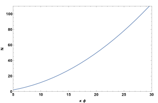
Figure 1: Plot of the number of e-folds as a function of the scalar field $\phi$ for $\xi=-0.0025$ and $\lambda=0.13$.

The spectral index of the power spectrum given by Eq.$\eqref{eq4.28}$, can be written as follow

$$n_{s} = 1-\frac{32\xi F}{16\xi N-(1-6\xi\omega-4\xi)(\sqrt{1+\frac{32\xi(1-6\xi\omega)}{(1-6\xi\omega-4\xi)}}-1)}(1-\frac{\xi\kappa^{2}\phi^{2}}{F})(1-\frac{\xi\kappa^{2}\phi^{2}}{2F})$$ (59)

$$+ \frac{2}{(1-6\xi\omega)}[\frac{3F}{\kappa^{2}\phi}-2\xi\omega-\kappa_{eff}((1+2\xi-4\xi\omega)\dot{\phi}-2\xi(1+\omega)H\phi)\frac{(1-6\xi\omega)H\dot{\phi}-2\xi\omega H^{2}\phi}{FH^{3}}].$$

Figs. 2(a) and 2(b) illustrate the evolution of $n_{s}$ for $\lambda=0.13$ and for different values of the coupling constant $\xi$. We plot the spectral index against the number of e-folds N and against the scalar field, respectively. The horizontal red line in both figures represents the upper bound for the spectral index imposed by Planck data. We conclude that the predictions of $n_{s}$ are consistent with Planck data.

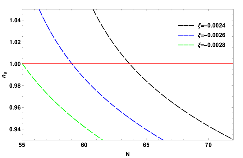
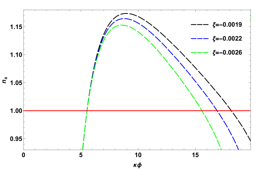
(a)

(b)

Figure 2: Evolution of $n_{s}$ as a function of the number of e-folds and as a function of the scalar field $\phi$ for different values of the coupling constant $\xi$ and $\lambda=0.13$ .

From Eq.(46) and Eq.(49), we get the power spectrum of the curvature perturbations

$$A^{2}_{s}=\frac{\kappa^{6}\lambda}{75\pi^{2}}\frac{\phi^{6}}{64}\frac{(1-6\xi\omega)^{2}}{(1+\xi\kappa^{2}\phi^{2})\left[1+\frac{C\kappa^{2}}{2F(\phi)H}\dot{\phi}\phi\right]^{2}},$$ (60)

and the tensor perturbations amplitude

$$A^{2}_{T}=\frac{\kappa^{4}\lambda}{75\pi}\frac{\phi^{4}}{1+\xi\kappa^{2}\phi^{2}}.$$ (61)

respectively. From Eq.$\eqref{eq5.6}$, we find that the tensor to scalar ratio can be obtained as

$$r=\frac{128\pi\xi}{(1-6\xi\omega)}\frac{\left[1+\frac{C\kappa^{2}}{2F(\phi)H}\dot{\phi}\phi\right]^{2}}{16\xi N-(1-6\xi\omega-4\xi)(\sqrt{1+\frac{32\xi(1-6\xi\omega)}{(1-6\xi\omega-4\xi)}}-1)}.$$ (62)

In Fig. 3, we present the evolution of r versus the number of e-folds N for $\lambda=0.13$ and for different values of the coupling constant $\xi$. Fig. shows also the upper bound (the red horizontal line) to the tensor to scalar ratio imposed by Planck data [1]. We notice that r lies within this bound in the range of N for selected values of $\xi$.

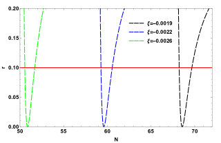
Figure 3: Variation of r against the number of e-folds N for three values of the coupling constant $\xi$ and for $\lambda=0.13$ .

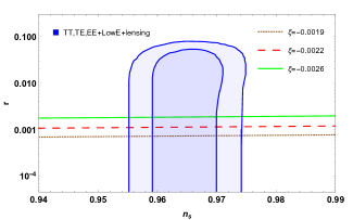
Figure 4: Variation of the tensor to scalar ratio r against the scalar spectral index $n_{s}$ for tree values of the coupling constant and $\lambda=0.13$.

In addition, from Fig. 4, where we plot the $(n_{s},r)$ plane for different values of the coupling constant $\xi$ in the range of number of e-folds $50<N<70$ with the constraints from the Planck TT,TE,EE+LowE+lensing, we can see that the predicted parameters are consistent with the observational data, where the value of the tensor to scalar ratio is $r\simeq 0.001$.

VII conclusions

In this work, we have studied a cosmological model where the field is non-minimal coupled with gravity in the hybrid metric Palatini approach.

We have also analyzed the cosmological perturbations in order to determine the different parameters during the inflationary period. As we have already mention, the existence of correction terms to the standard background and perturbative parameters, represents the impact of the Palatini approach and the non-minimal coupling between the field and the Ricci scalar.

We have applied our model by developping in detail a non-minimally coupled inflationary model driven by the Higgs field with a quadratic potential, within the slow-roll approximation.

We have checked our results by plotting the evolution of different inflationary parameters versus the constraints provided by the observational data as shown in the Figs. 2, 3 and 4.

We have found that the perturbed parameters such as the tensor to scalar ratio and the scalar spectral index are compatible with the observational data, for a number of e-folds $N\in[50;70]$ for three values of $\xi$ as Figs. 2 and 3 show.

Finally, for more checking of consistensy of our model, we have compared our theoretical predictions with observational data [1] by plotting the Planck confidence contours in the plane of $n_{s}-r$ as we can see in Fig. 4. The results show that the predicted parameters are in good agreement with the Planck data, in the range of the number of e-folds $50-70$ for selected values of NMC constant $\xi$.

References

• [1] Y. Akrami et al. [Planck Collaboration], [astro-ph.CO/1807.06211].
• [2] A. A. Starobinsky, Phys. Lett. B 91, 99 (1980).
• [3] A. D. Linde, Phys. Lett. B 129, 177 (1983).
• [4] K. Sato, Mon. Not. R. Astron. Soc. 195, 467 (1981).
• [5] A. D. Linde, Phys. Lett. B 108, 389 (1982).
• [6] A. Guth, Phys. Rev. D 23, 347 (1981).
• [7] A. Albrecht and P. J. Steinhardt, Phys. Rev. Lett. 48, 1220 (1982); A. Linde, Particle Physics and inflationary cosmology (Gordon and Breach, New York, 1990).
• [8] V. F. Mukhanov and G. V. Chibisov , JETP Letters 33, 532 (1981).
• [9] S. W. Hawking, Phys. Lett. B 115, 295 (1982).
• [10] A. Guth and S.-Y. Pi, Phys. Rev. Lett. 49, 1110 (1982).
• [11] A. A. Starobinsky, Phys. Lett. B 117, 175 (1982).
• [12] J. M. Bardeen, P. J. Steinhardt and M. S. Turner, Phys. Rev. D 28, 679 (1983).
• [13] C. L. Bennett et al., Astrophys. J. Suppl. 192, 17 (2011).
• [14] G. Hinshaw et al. [WMAP Collaboration], Astrophys. J. Suppl. 208, 19 (2013), [arXiv:1212.5226].
• [15] P. A. R. Ade et al. [Planck Collaboration], [arXiv:1303.5082].
• [16] E. Komatsu et al., [WMAP collaboration], Astrophys. J. Suppl. 192, 18 (2011) [arXiv:1001.4538]; B. Gold et al., Astrophys. J. Suppl. 192, 15 (2011) [arXiv:1001.4555].
• [17] D. Larson et al., Astrophys. J. Suppl. 192, 16 (2011) [arXiv:1001.4635].
• [18] A. Bargach, F. Bargach, M. Bouhmadi-López, and T. Ouali. Phys. Rev. D 102, 123540 (2020).
• [19] Cervantes-Cota, Jorge L and Dehnen, H. Nuclear Physics B 442, 391–409 (1995).
• [20] F. L. Bezrukov and M. Shaposhnikov, Phys. Lett. B 659, 703–706 (2008) [hep-th/0710.3755].
• [21] M. U. Rehman and Q. Shafi, Phys. Rev. D 81 (2010) 123525 [astro-ph.CO/1003.5915].
• [22] F. Bezrukov, D. Gorbunov, C. Shepherd and A. Tokareva, Phys. Lett. B 795, 657 (2019) [hep-ph/1904.04737].
• [23] S. Raatikainen and S. Rasanen, JCAP 1912 (2019) no.12, 021 [gr-qc/1910.03488].
• [24] S. Rasanen and P. Wahlman, JCAP 11, 047 (2017) [arXiv:1709.07853 [astro-ph.CO]].
• [25] V. M. Enckell, K. Enqvist, S. Rasanen and E. Tomberg, JCAP 06, 005 (2018) [arXiv:1802.09299 [astro-ph.CO]].
• [26] F. Bauer and D. A. Demir, Phys. Lett. B 698, 425-429 (2011) [arXiv:1012.2900 [hep-ph]].
• [27] J. Rubio, Front. Astron. Space Sci. 5, 50 (2019) [arXiv:1807.02376 [hep-ph]].
• [28] T. Tenkanen, Gen. Rel. Grav. 52, 1–24 (2020) [arXiv:2001.10135 [astro-ph.CO]].
• [29] S. Capozziello, T. Harko, T. S. Koivisto, F. S. N. Lobo and G. J. Olmo, Universe 1, 199 (2015).
• [30] C. Fu, P. Wu, and H. Yu, Phys. Rev. D 96, 103542 (2017).
• [31] F. Melia, Mod. Phys. Lett. A 37, 2250016 (2022).
• [32] J. M. Bardeen, Phys. Rev. D 22, 1882 (1980).
• [33] ] V. F. Mukhanov, H. A. Feldman, and R. H. Brandenberger, Phys. Rept. 215, 203 (1992).
• [34] Bardeen, J. M., Steinhardt, P. A., and Turner, M. S, Phys. Rev. D 28, 679(1983).
• [35] C. Deffayet, Phys. Rev. D 66, 103504 (2002), [arXiv:hep-th/0205084].
• [36] L. Amendola, C. Charmousis and S. C. Davis, JCAP 0612, 020 (2006), [hep-th/0506137].
• [37] L. Amendola, C. Charmousis and S. C. Davis, JCAP 0710, 004 (2007), [astro-ph/0704.0175].
• [38] S. Rasanen and E. Tomberg, JCAP 1901, 038 (2019), [astro-ph.CO/1810.12608].
• [39] K. Nozari and N. Rashidi, Phys. Rev. D 88, 023519 (2013).
• [40] B. A. Bassett, S. Tsujikawa and D. Wands, Rev. Mod. Phys. 78, 537 (2006).
• [41] Riotto, ICTP Lect. Notes Ser. 14, 317 (2003), [hep-ph/0210162].
• [42] K. Nozari and N. Rashidi, Phys. Rev. D 86, 043505 (2012).