À Propos Crossing the Hertzsprung Gap

Abstract

The evolution of intermediate-mass and massive stars speeds up considerably after they finish their hydrogen core-burning. Due to this accelerated evolution, the probability to observe stars during this episode is small. In suitable stellar aggregates, in particular star clusters of appropriate ages, the fast evolutionary phase causes a depopulated area – referred to as the Hertzsprung gap – in color-magnitude diagrams and derivatives therefrom. The explanation of the speed-up usually resorts to the star’s Kelvin-Helmholtz timescale and the Schönberg-Chandrasekhar instability is called upon. This exposition challenges this viewpoint with counterexamples and argues that a suitably defined nuclear timescale is enough to explain the fast evolution. A thermal instability, even though it develops in stars evolving through the Hertzsprung gap, is not a necessary condition to trigger the phenomenon.

CBmA, 4410 Liestal, Switzerland

1 Introduction

Color-magnitude diagrams – and therefore also the Hertzsprung-Russell (HR) diagrams resorted to in the following – of suitably chosen stellar aggregates often show a region, originally specified as between early A-type and late G-type stars, which is only scarcely populated. The laudatio of Phillips (1929), on the occasion of awarding the Gold Medal of the Royal Astronomical Society to Hertzsprung, reviewed concisely the pertinent work of awardee to establish the reality of a gap in the distribution of the stars as a function of spectral type. It was the paper of Strömberg (1932) through which the expression ‘Hertzsprung gap’ found its way to the astronomical literature. Figure 1 illustrates the phenomenon using a modern mixed color-magnitude/Hess diagram comprised of the brighter stars within 250 pc of the sun that were measured with the astrometric space mission Gaia. The observed Hertzsprung gap is marked with the grey wedge added to the upper left of the diagram.

Color-magnitude diagram from the stars within 250 pc around the sun as observed with Gaia and made available in DR2. The grey wedge in the upper left hints at the region referred to as the Hertzsprung gap.

In the early 1950s when the general direction of a star’s evolution became clear (cf. Sandage & Schwarzschild, 1952), it was realized that the Hertzsprung gap is a region through which sufficiently massive stars evolve comparatively fast after hydrogen is exhausted in their cores. The higher evolutionary speed lowers hence the probability to catch stars during that episode. Already early on, the origin of the speed-up was conjectured to be connected with the Schönberg-Chandrasekhar (SC) instability.

At the end of the main-sequence phase, i.e. when the stellar cores run out of nuclear fuel, the stars adjust their structure as the nuclear burning shifts to a shell on top of a nuclear inactive core. At first, the shell is fat but it grows ever thinner as the star approaches the base of the first giant branch (FGB). In the absence of nuclear burning no luminosity is generated and hence the temperature gradient in the core vanishes also – at least in the clinically clean case of a star in full equilibrium. If the core contracts, on the other hand, a small temperature gradient is maintained. In particular for intermediate-mass and massive stars, the core must contract once it grows too massive. If the relative core mass, $q$, exceeds roughly $0.1$, the SC-instability (e.g. Kippenhahn et al., 2012) predicts the shrinking and an accompanying heating of the inert stellar core. The SC thermal instability is usually linked to the Kelvin-Helmholtz timescale of the star.Gabriel & Ledoux (1967) were the first to do a full secular stability analysis of stellar structures that correspond to the original SC model setup. Ledoux (1969) felt convinced that the fast evolution connecting the terminal main-sequence and the early FGB phase was due to the identified secular instability. Even if not stated expressis verbis, the students tend come away from the textbooks with the conceptual thread ‘Hertzsprung gap’ – ‘Kelvin-Helmholtz timescale’ – ‘SC-instability’. But is this really a causal chain? This question has been contemplated and debated repeatedly in the past (e.g. Lauterborn & Siquig, 1976; Spindler & Lauterborn, 1977; Hansen, 1978, and references therein). The answers pointed mostly to a circumstantial connection of the SC instability and the evolutionary speed-up of the stars across the HR plane.

The following exposition presents the results of counterexamples to the reasoning of thermal instability being the cause of the speed-up. Even though hardly anything is new, the discussion and the compilation of facts put forth should help students of the stars to shape their understanding of the phenomenon and hopefully allows them to proceed beyond where we currently stall. An appendix is devoted to the presentation of canonical secular stability computations, which are referred to in the main text, addressing their usefulness and their limitations. In contrast to the older literature, the acquired stability results are comprehensive enough to illustrate how the lowest-order secular modes evolve and interact.

2 Stellar Evolution from the ZAMS to the FGB

The evolutionary tracks on the HR Diagram of the intermediate-mass and massive model stars ($2.5<M_{\ast}/M_{\odot}<10$) that were studied for this note are shown in Fig. 1. The thin black lines trace the MESA-computed quasi-hydrostatic evolution (QHE). The QHE computations were arbitrarily stopped along the FGB at central helium ignition. The stars’ initial homogeneous composition was set to $(X,Z)=(0.7,0.02)$. Boundaries of the convection zones were determined using Ledoux’s criterion.[-1.5cm]Further choices in the &controls inlist were: mixing_length_alpha=1.8 and for some mild overshooting: overshoot_f$\langle\ast\rangle$=0.012 overshoot_f0$\langle\ast\rangle$=0.002 with the wildcard $\langle\ast\rangle$ covering all necessary subspecifications. The particular choices to model the stars change the numerical values of the results presented here but not their qualitative behavior.

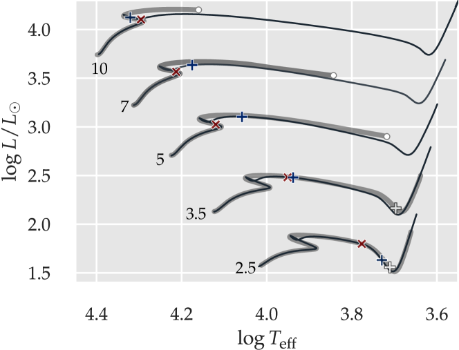
Figure 1: A collection of evolutionary tracks of intermediate-mass and massive stars in QHE (thin back) and FE (thick grey lines) approximation. The stars’ masses in solar units are labeled along the ZAMS. The meaning of the crosses and the white circles is elaborated in the text.

Additionally, the evolution of stars in full equilibrium (FE), i.e. imposing ${\mathrm{d}}_{t}Q\equiv 0$ in the energy equation, was calculated for the same set of stellar masses (heavy grey lines in Fig. 1). The computation of two lowest-mass FE tracks was stopped arbitrarily once the stars started to ascend the FGB. The white crosses along the lower-mass FE model evolutionary tracks mark the epochs when a monotonic secular instability[][-3mm]computed with the linear perturbation analysis discussed in the Appendix sets in. Evidently, the computation of these two lower-mass FE model sequences was not impeded by the instability of the lowest-order secular mode. The higher-mass models ($M_{\ast}>3.5\,M_{\odot}$), on the other hand, stalled – indicated by a white circle at the end of the respective tracks – when the Henyey-type solver failed to converge. In FE modeling, this computational breakdown is attributed to the onset of a monotonic thermal instability of the model once the uniqueness of the equilibrium solution is violated (cf. Gabriel & Ledoux, 1967; Paczyński, 1972). At least for sufficiently low stellar masses, MESA in FE-mode is apparently able to proceed past the onset of a monotonic thermal instability. In MESA, the stellar structure equations are solved simultaneously with those of the nuclear network and the mixing of nuclear species (see Fig.47 in Paxton et al., 2013). Therefore, depending on the number of explicitly treated species,The computations in this study used the approx21.net network. The compositional subspace entering the Henyey matrix,

$$\frac{\mathrm{d}(\mathrm{chem}_{k})}{\mathrm{d}(\mathrm{chem}_{k})}\in M(21\times 21)\,,$$

in Paxton et al. (2013) notation, is considerably larger than the structural $M(4\times 4)$ one. The subscript refers to cell $k$ of the spatial discretization. the size of a Henyey block can be considerably larger than in the traditional stellar evolution codes. Even if the determinant of the ‘structure subspace’ – matrix vanishes once a real secular eigenvalues passes through zero, the determinant of the total Henyey matrix may, nonetheless, remain nonzero due to the effect of the compositional subspace. The detailed reason of why lower-mass FE model stars avoid stalling at the onset of the monotonic secular instability after their main-sequence phase but the more massive siblings fail remains to be understood.

The red crosses ($\times$) in Fig. 1 mark the epochs when the relative helium core-mass exceeds $q_{\mathrm{core}}=0.1$. This choice of $q_{\mathrm{core}}$ was motivated by the magnitude usually quoted when ideal-gas model envelopes fail to match isothermal cores, i.e. when the SC instability is encountered in respective simple model stars. The $5$ to $10\,M_{\odot}$ sequences shown in Fig. 1 start their hydrogen-free core evolution with a helium core whose mass already exceeds $q_{\mathrm{core}}=0.1$. The red crosses mark therefore the epochs of the emergence of inert pure helium cores that are initially already SC super-critical.

Finally, the blue crosses ($+$) mark the onset of the monotonic secular instability as obtained from linear secular stability computations (see Appendix) performed on QHE models, this is the instability that is usually associated with the SC instability (e.g. Kähler, 1972). The secular eigenanalyses covered the evolutionary stages from the ZAMS to the lower FGB. Red edges of the unstable monotonic modes were not encountered in any of the sequences.

To quantify the depopulation of stars along the effective-temperature axis we introduce the transverse evolution timescale of stars across the HR diagram as:

$$\tau_{T_{\rm eff}}=\frac{\Delta t}{\left|\Delta\ln T_{\rm eff}\right|}\,.$$

[-1cm]for some suitably chosen time interval $\Delta t$ and the accompanied $\Delta T_{\rm eff}(\Delta t)$ The quantity $\tau_{T_{\rm eff}}$ measures how efficiently stars get plowed out of selected temperature/color bins. If a star evolves mostly horizontally in the HR diagram then $\tau_{T_{\rm eff}}$ is even an indicator of the overall evolution timescale on that plane.

$$\tau_{\mathrm{evol}}=\frac{\Delta t}{\left(\left|\Delta\ln L\right|^{2}+\left|\Delta\ln T_{\rm eff}\right|^{2}\right)^{1/2}}\,.$$

On the other hand, if also a star’s luminosity changes significantly, $\tau_{T_{\rm eff}}$ still serves as an upper bound of the evolution timescale. This latter case is encountered at low effective temperatures of lower-mass stars where $\tau_{T_{\rm eff}}$ first remains high because it is blind to the luminosity drop before the base of the FGB is reached. For higher stellar masses this discrepancy shrinks as illustrated in Fig. 1.

Variation and comparison of characteristic timescales during the post main-sequence evolution. The transverse timescale, $\tau_{T_{\rm eff}}$ (blue), is the upper bound to the evolutionary timescale, $\tau_{\rm{evol}}$ (black), which accounts also for the luminosity change. The black peaks touching the $\tau_{T_{\rm eff}}$ loci at low $T_{\rm eff}$ mark the base of the FGB when the stars’ luminosity passes through a local minimum. The $\tau_{T_{\rm eff}}$ behavior associated with the QHE evolutionary tracks displayed in Fig. 1 is collected in Fig. 2. The stars enter the diagram on the top left of the respective loci after they have taken the first turn of their S-bend evolution; i.e. when the stars’ central furnace runs out of hydrogen. The first speedy evolution episode develops while stars evolve through the second turn of the S-bend (the bowl-shaped episode in Fig. 2) while the hydrogen-burning shell develops. For stars more massive than about $2.5\,M_{\odot}$ the post – S-bend evolution to lower effective temperatures gets progressively faster towards the base of the FGB where $\tau_{T_{\rm eff}}$ passes through a local minimum. For the set of computed evolutionary tracks the margin table reports the maximum speed-up of the stars’ evolution relative to the epoch around the end of their S-bend phase. Notice that the speed-up by a factor two in the $2.5\,M_{\odot}$ model sequence is reached already shortly after the end of the S-bend passage. The subsequent evolution to the base of the FGB is mostly slower than that through the S-bend. Together with the inspection of Fig. 2 we deduce that – for the set of parameters chosen for this study – the Hertzsprung-gap develops for stars more massive than about $2.5\,M_{\odot}$. After $\tau_{T_{\rm eff}}$ evolved through its local minimum at low effective temperatures it eventually forfeits its usefulness because the steep luminosity rise dominates the stars’ evolution along the FGB (cf. Fig.1). [-4cm] Mass/$M_{\odot}$ max. transverse speed-up 2.5 2 3.5 3.5 5 10 7 25 10 40

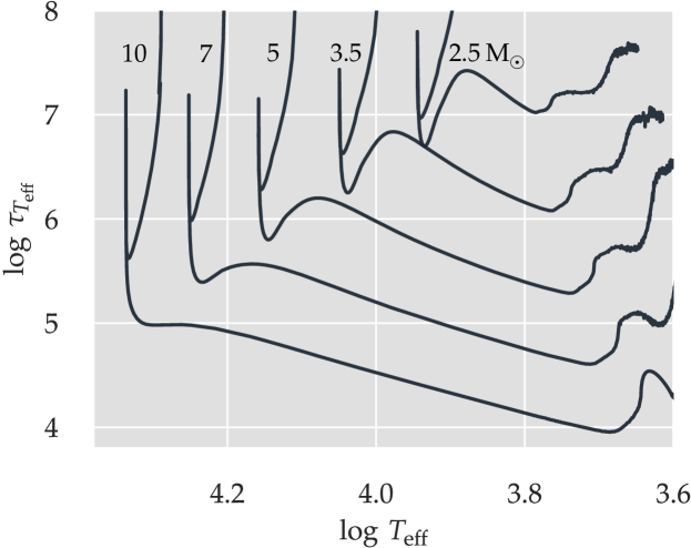
Figure 2: The variation of the timescale $\tau_{T_{\rm eff}}$, a measure of the magnitude of transverse evolution across the HR diagram, for the QHE model sequences presented in Fig. 1. After their first turn of the S-bend evolution the model stars enter the diagram at the top. For all models more massive than about $2.5\,M_{\odot}$, $\tau_{T_{\rm eff}}$ drops significantly, i.e. evolution speeds up, when they develop their H-shell burning and evolve to the base of the FGB.

Evidently, Fig. 2 and the rough quantification in the margin-table illustrate how QHE modeling accounts for the relative scarcity of stars in the Hertzsprung gap of the HR diagrams. The QHE models predict qualitatively that for stellar masses $\gtrsim 2.5M_{\odot}$ depopulation starts close to the main sequence band. With increasing mass, at higher luminosity hence, the gap broadens. The lowest $\tau_{T_{\rm eff}}$ is encountered close to the base of the FGB.

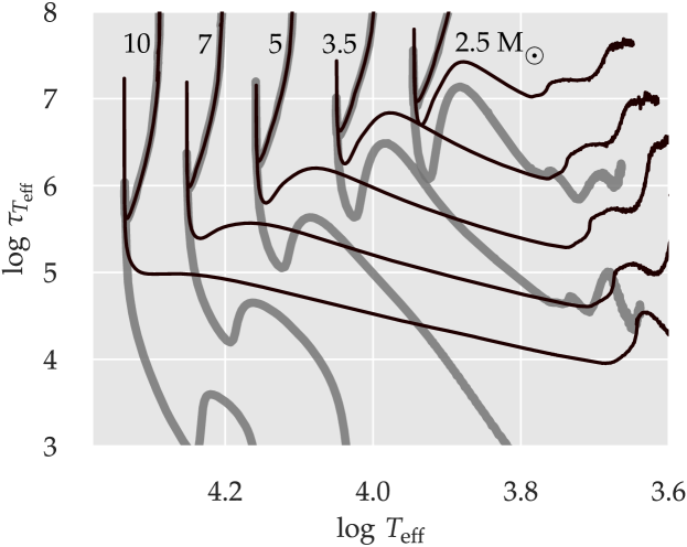
Figure 3: Comparing the QHE-models’ $\tau_{T_{\rm eff}}$ (thin black lines) with those of the respective FE-models (thick grey lines) reveals the latter to evolve even faster across the HR plane than their QHE brethren.

The QHE tracks and the associated transverse evolutionary timescales account the Hertzsprung gap. If the origin of the accelerated evolution after central H-burning is indeed caused by a thermal instability (which is present in the QHE ansatz via the ${\mathrm{d}}_{t}Q$ term in the energy equation) then post – main-sequence evolution should slow down in the FE approximation. Thanks to MESA’s property to evolve model stars in FE mode, we could follow lower-mass stars ($M_{\ast}\lesssim 3.5M_{\odot}$) even up the lower FGB and the more massive model sequences at least to the onset of their secular instability. Therefore, MESA offers the unique opportunity to compare FE $\tau_{T_{\rm eff}}$ values to the respective QHE numbers over a pertinent range of evolutionary stages. Figure 3 shows again the set of $\tau_{T_{\rm eff}}$ loci of the QHE evolution as thin black lines and those from FE evolution superimposed as heavy grey lines. The correspondence of QHE and FE loci are evident because they are essentially identical to the end of the S-bend evolution. Once the H-burning shell developed, FE-evolution across the HR plane is, for all masses considered, always faster than the corresponding QHE one.This was pointed out already by Roth (1973) Since ${\mathrm{d}}_{t}Q=0$ underlies the FE models, the fast FE evolution cannot be attributed to thermal imbalance and hence is not caused by a thermal instability. Apparently, thermal imbalance slows down post – main-sequence evolution as compared to models in thermal equilibrium.

Even though we tried to get away from correlations, the transverse evolutionary timescales be compared in the following to some timescales canonically resorted to in stellar astrophysics: Figure 4 compares for the representative $2.5\,M_{\odot}$ and $7\,M_{\odot}$ tracks the models’ nuclear timescale, $\tau_{\mathrm{Nuc}}$ (Nuc), a suitably defined local nuclear timescale, $\tau_{\mathrm{Nuc/loc}}$ (Nuc/loc), the Kelvin-Helmholtz timescale, $\tau_{\mathrm{KH}}$ (KH), of the complete stars, and the Kelvin-Helmholtz timescale of the cores only, $\tau_{\mathrm{KHc}}$ (KHc):

$$\tau_{\mathrm{Nuc}} =1\cdot 10^{10}\frac{M_{\ast}/M_{\odot}}{L_{\ast}/L_{\odot}}\,,$$

$$\tau_{\mathrm{Nuc/loc}} =\left|\frac{X}{\dot{X}}\right|_{\varepsilon_{\mathrm{max}}}\,,$$

$$\tau_{\mathrm{KH}} =3\cdot 10^{7}\frac{(M_{\ast}/M_{\odot})^{2}}{(R_{\ast}/R_{\odot})(L_{\ast}/L_{\odot})}\,,$$

$$\tau_{\mathrm{KHc}} =3\cdot 10^{7}\frac{(M_{\mathrm{core}}/M_{\odot})^{2}}{(R_{\mathrm{core}}/R_{\odot})(L_{\mathrm{core}}/L_{\odot})}\,.$$

The nuclear timescale simply measures the time it takes for a certain fraction of a star’s hydrogen to be converted to helium. The numerical factor in $\tau_{\mathrm{Nuc}}$ results from ad hoc assuming $10\%$ of the star’s hydrogen to be converted to helium at the prevailing luminosity. Once a star derives its energy from an ever thinner nuclear burning shell, the concept of the local nuclear timescale seems more appropriate than the crude $\tau_{\mathrm{Nuc}}$ measure. Here, the local nuclear timescale measures the time it takes to burn away a fraction of the fuel in the nuclear active shell with the physical quantities being evaluated at the maximum of the nuclear energy generation rate, $\varepsilon_{\mathrm{max}}$, of the burning shell. Its unsteady temporal runs seen in Fig. 4 are owed to the spatial gridding and adopting $\varepsilon_{\mathrm{max}}$ at the respective computational cell, rather than spatially interpolating the maximum. The abundances are derived at the cell with the maximum nuclear energy generation rate. Depending on the motion of this maximum across the computational grid and the shifting convection boundaries, small jumps are inflicted. The $\tau_{\mathrm{Nuc/loc}}$ definition serves as a lower bound of this timescale because per definitionem nuclear burning is assumed to operate at maximum magnitude in an actually sharply peaked burning shell. The global Kelvin-Helmholtz timescale, $\tau_{\mathrm{KH}}$, measures the time available to support a star’s luminosity when tapping its internal energy only. Restricting the radiating sphere to the inert helium core of a shell-burning star leads to the definition of the Kelvin-Helmholtz timescale of the core, $\tau_{\mathrm{KHc}}$. The e-folding times of the unstable monotonic secular mode(s) (Sec) are displayed as dark-red dots. Finally, the continuous blue $\tau_{T_{\rm eff}}$ curve (Te) shows how the transverse effective-temperature evolution of the model stars compares to the other timescales.

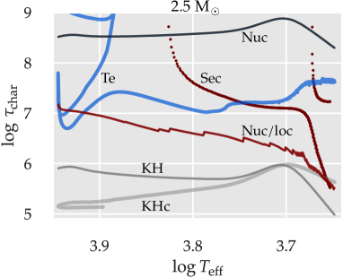
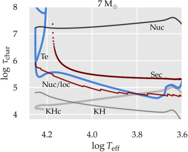
Figure 4: Comparison of various timescale concepts along two representative evolutionary paths. The left panel shows the case of the $2.5M_{\odot}$ star at the low-mass boundary of the Hertzsprung gap; the right panel that of the $7M_{\odot}$ one. The meaning of nuclear (Nuc), local nuclear (Nuc/loc), Kelvin-Helmholtz (KH), secular (Sec), and the transverse evolution timescales are discussed in the text.

In both panels of Fig. 4, the blue $\tau_{T_{\rm eff}}$ (Te) loci of the post – main-sequence phases of the $2.5\,M_{\odot}$ sequence on the left and the $7\,M_{\odot}$ track on the right are generously sandwiched between $\tau_{\mathrm{Nuc}}$ (Nuc) and $\tau_{\mathrm{KH}}$ (KH). Evidently, $\tau_{\mathrm{Nuc}}$ is much too long and $\tau_{\mathrm{KH}}$ is significantly too short. The red $\tau_{\mathrm{Nuc/loc}}$ (Nuc/loc) lines on the other hand agree better with the stars’ evolution across the Hertzsprung gap. This applies particularly well to the more massive example where a significant speed-up is observed for the model stars between the end of the S-bend and the FGB. The worsening agreement of the temporal evolution of $\tau_{T_{\rm eff}}$ and $\tau_{\mathrm{Nuc/loc}}$ during the $2.5\,M_{\odot}$ model’s approach of the base of the FGB mostly is partially attributable to the luminosity drop (Fig. 1), which is not accounted for in the $\tau_{T_{\rm eff}}$ (Fig. 1) definition. The timescale behaviors of the $7\,M_{\odot}$ example of the right panel of Fig. 4 are representative of all evolutionary sequences with significant speed-up after their main-sequence phase.

The dark red points (Sec) added to Fig. 4 trace the e-folding times of the unstable monotonic secular mode customary associated with the SC-instability. The blue edge of the linear instability region lies at the divergence to infinity of the e-folding time. Red edges were not encountered in any of the analyzed model sequences. As to be expected, the secular e-folding times are much shorter than the nuclear timescale but they are also considerably longer than $\tau_{\mathrm{KH}}$ the Kelvin-Helmholtz timescale of the complete star. In the case of the $2.5\,M_{\odot}$ sequence, the e-folding time of the secular instability and $\tau_{\mathrm{KH}}$ become comparable only around the base of the FGB.[][-1.8cm]The enhanced instability is induced by an avoided crossing of the originally unstable secular mode with a mode from a subspectrum that develops as the model sequence evolves through the base of the FGB. See Fig. 5. Hence, most of the Hertzsprung gap is crossed faster than what the unstable secular mode supports. On the other hand, in the post – main-sequence evolution of the $7\,M_{\odot}$ star, the e-folding time of the unstable secular mode is comparable with $\tau_{T_{\rm eff}}$ on the hot side of the Hertzsprung gap. However, during the crossing of the gap, the timescale of the secular mode remains longer than that of the transverse evolution. Even a comparison with $\tau_{\mathrm{KHc}}$ (KHc), the Kelvin-Helmholtz timescale of the inert stellar core does not help. In the case of the $2.5\,M_{\odot}$ evolution $\tau_{\mathrm{KHc}}$ is mostly shorter than $\tau_{\mathrm{KH}}$. Even if $\tau_{\mathrm{KHc}}$ exceeds $\tau_{\mathrm{KH}}$ and approaches $\tau_{T_{\rm eff}}$, its temporal functional variation does not match that of $\tau_{T_{\rm eff}}$. Therefore, there is no obvious reason to conjecture that thermal behavior of the inert core drives the rapid evolution across the HR plane.

The most important aspect here is that neither the e-folding time of the unstable secular mode nor the Kelvin-Helmholtz timescale of neither the complete star nor the core alone do correlate with the $\tau_{T_{\rm eff}}$ evolution. In particular, the model stars evolve fast already before any secular instability unfolds (in the QHE case) or even without any secular instability being possible (in the FE case).

An FE model can be thought of consisting of an inert, isothermal core of specified mass and a radiative-zero envelope (at least for sufficiently hot model stars).[][-5cm]Except for the partial ionization regions close to the stellar surface, the FE and also the QHE envelopes both admit ${\mathrm{d}}\log T/{\mathrm{d}}\log P\approx 0.23$, which is close to a radiative-zero solution. Early on, during the post – S-bend evolution the stars are hot enough so that the partial ionization regions and the accompanying convection zones are very thin and therefore without significant effect on the global envelope structure. The two regions are separated by a nuclear-burning shell. The close proximity of evolutionary tracks of FE and QHE models across the Hertzsprung gap means that both respective envelopes transport roughly same luminosity. In QHE models, nuclear energy generation produces a higher luminosity than in FE models at the same location on the HR plane. Some of energy goes into the expansion of the envelope so that the surface luminosity of the FE and QHE models are eventually roughly the same (as it is reflected in the very similar computed envelope structures). Hence, the reason of the different timescales of their evolution through the Hertzsprung gap must be sought in the properties of the nuclear-burning shell and possibly their effect on the stellar radius.

Structural difference at around the H-burning shell of $5\,M_{\odot}$ QHE (black) and FE (red) models at $\log T_{\rm eff}=3.8$.

In FE models, the nuclear-burning shell alone must adapt in such a way as to supply the required transportable energy flux at the base of the envelope. Because of the developing isothermal core (bottom panel in Fig. 4) and the steeper temperature gradient on top of it most of the luminosity is generated at the very inner edge of $X$-abundance ramp (cf.second panel from the bottom in Fig. 4 where $X<{\cal O}(10^{-3})$). Apparently, the nuclear shell source of FE models is not as strong as that in comparable QHE ones but it is more massive so that eventually about the same surface luminosity results. The top panel of Fig. 4 shows the FE-luminosity in red, the nuclear luminosity of the QHE model in grey and the total luminosity as a fine black line. The latter contains the contribution from the star’s contraction/expansion, which is well expressed around the H-burning shell. At the surface of the model star displayed in Fig. 4, the thin black line drops even slightly below the red one. Because $X|_{\varepsilon_{\mathrm{max}}}$ is much smaller in FE models than in QHE ones, their lateral timescale ($\tau_{\mathrm{Nuc/loc}}\sim X/\varepsilon_{\mathrm{Nuc}}$) is accordingly shorter. This means that FE models evolve even faster than QHE ones.

Early into the post-ms evolution, the mass of the H-burning shell increases with stellar mass. The difference in mass diminishes as the stars approach the base of the FGB. Hence, the thinner the nuclear burning shell the shorter the local nuclear timescale, the faster the star’s evolution between the end of hydrogen core-burning and the FGB. Therefore, evolution to the base of the giant branch of the lower-mass stars is comparatively slower.

Even though the usefulness of linear secular stability analyses is limited or even questionable during fast evolutionary phases we resorted to them here. The Appendix at the end of this exposition is devoted to a presentation of the mode diagrams encountered in secular eigenmode analyses and more importantly to tests performed with MESA illustrating how well (or badly) a linear stability analysis does during the speedy evolution through the Hertzsprung gap.

Summary

The evolution of intermediate-mass and massive stars speeds up significantly after the S-bend at the end of the main-sequence phase and the base of the FGB. The resulting scarcity of stars on the HR plane during this evolutionary phase is known as the Hertzsprung gap. We showed that also stars in full equilibrium speed up on the HR plane once a H-burning shell develops. Even though a water-tight proof is still pending the results suggest that the development of the Hertzsprung gap does not depend on a thermal/secular instability. The fast evolution across the HR plane can be attributed to the properties of the ever thinner H-burning shell at the base of the stars’ envelopes alone. Hence, the SC instability is rather a secular instability that develops on top of independently ever faster evolving stars. Because MESA solves the equations of stellar structure and chemical composition simultaneously it is able to track FE models longer than the older generations of stellar evolution codes that decoupled stellar structure and nuclear evolution. The comparison of the QHE and the FE tracks of intermediate-mass model stars computed with MESA show that they remain close to each other. Hence, once it develops, the SC secular instability does not significantly affect the stars’ evolutionary locus on the HR plane. Even though the stellar luminosity profiles are locally affected by the secular instabilities, the stars’ loci on the HR plane are very similar for QHE and FE models, respectively. The FE models (where they exist in the Hertzsprung gap) evolve even faster than the QHE siblings. Hence the speed-up cannot be attributed to a thermal instability of post – main-sequence stars.

Acknowledgments: Access to NASA’s Astrophysics Data System was indispensable to write this exposition. Figure 1 relies on data from the European Space Agency (ESA) mission Gaia, which is processed by the Gaia Data Processing and Analysis Consortium (DPAC). Funding for the DPAC has been provided by national institutions, in particular the institutions participating in the Gaia Multilateral Agreement. The python code listed in a 2018 blog post of Vlas Sokolov (https://vlas.dev/post/) served as a helpful template to efficiently start querying the Gaia DR2 database to produce Fig. 1. The model stars were computed with the Modules for Experiments in Stellar Astrophysics (MESA, Paxton et al., 2018, and references therein) mostly in version $12\,115$.

This installment is dedicated to the memory of P. Freiburghaus, aka H.H. – he was an invaluable source of inspiration.

3 Appendix

Secular stability of the model stars of the various evolutionary tracks was computed in the linear regime with the Riccati approach as described in Gautschy & Althaus (2007). Again, the QHE approximation was used, i.e. a simple perturbation of the ${\mathrm{d}}_{t}Q$ term was included in the secular stability problem; convection was treated as instantaneously adapted to its environment.

The structure of the secular mode diagrams of intermediate-mass and massive stars during hydrogen core- and shell-burning phase, representatively illustrated by the $2.5M_{\odot}$ star.[][-1.8cm]The temporal separation ansatz adopts $q(m;t)\propto\exp({\rm i}\sigma t)$ with $\sigma$ being possibly complex $(\sigma_{\rm R},\sigma_{\rm I})$ because the secular problem is not self-adjoint. The eigenfrequencies $\sigma$ are expressed in units of the star’s free-fall frequency.

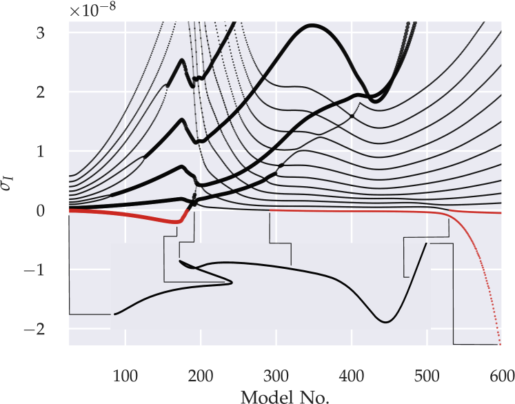
Figure 5: Secular mode diagram, imaginary parts of the eigenvalues as a function of model number along the evolutionary track of the $2.5\,M_{\odot}$ star inset at the bottom of the figure. Small circles mark monotonic eigenmodes ($\sigma=\left(0,\sigma_{\mathrm{I}}\right)$); the stronger filled circles indicate complex eigensolutions. Black colored eigenvalues mark damped modes, red ones unstable ones ($\sigma_{\mathrm{I}}<0$). For better orientation along the mode-number abscissa, a few pertinent epochs along the HR-track of the star point to the respective positions in the secular mode-diagram. Except for the avoided crossing in the lower right the mode diagram is representative for all evolutionary sequences computed for this exposition.

Already during the main-sequence phase of the star, the lowest two eigenmodes are complex, i.e. the two secular modes are oscillatory. The lowest mode is even weakly unstable. Except for the $10\,M_{\odot}$ sequence, this behavior has been found for all masses considered here. Despite reducing the evolutionary timesteps of MESA models well below the stars’ Kelvin-Helmholtz timescale during respective main-sequence phases, no evidence of an instability could be found in the evolution computations.

As evolution progresses along the main sequence, pairs of ever higher-order monotonic eigenmodes merge into complex eigensolutions as it has been reported in the literature for a long time (e.g. Aizenman & Perdang, 1971b). Once a star approaches the FGB, all $\sigma_{\rm I}$ tend to grow again. It is only the lowest monotonic secular eigenmode, i.e. the lower branch of the unfolded, initially complex eigenmode that goes unstable. In the case of the $2.5\,M_{\odot}$ sequence actually two secular modes are found unstable at the lower FGB. The mode of a secular subspectrum that develops during the shell-burning phase of evolution interacts with the mode family running almost horizontally in Fig. 5. At the avoided crossing with the lowest-order, already unstable secular mode the interfering mode picks up a large negative $\sigma_{\rm I}$ and develops into the dominantly unstable mode.

The way the lowest monotonic mode branch goes unstable is similar in all computed mass sequences: During the main-sequence phase, the lowest eigenmodes are complex, either already on the ZAMS or they merge into pairs during core hydrogen burning. The complex modes react only weakly on the restructuring of the star as nuclear burning shifts from center to a shell. When the nuclear-burning shell develops, an additional sub-spectrum of purely monotonic eigenmodes intrudes from large $\sigma_{\rm I}$ values to form a broad trough as the star evolves across the Hertzsprung gap. Also around the onset of shell burning, the lowest complex mode unfolds into a pair of monotonic modes with the lower-$\sigma_{\rm I}$ branch going unstable during the post S-bend evolution. It is this monotonic instability that is commonly associated with the SC-instability.

Fragmentary secular mode diagram for the $2.5\,M_{\odot}$ model track computed with the Schwarzschild criterion and without overshooting. N.B. the model numbers in the plot belong to different evolutionary epochs from those appearing in Fig. 5. Gabriel (1972) contemplated that the differences in the secular eigenspectrum of his study and the work of Aizenman & Perdang (1971a) might be attributable to differences in the central convection zones. Our standard setup in MESA relied on the Ledoux criterion with moderate overshooting at the convective boundaries. To scrutinize the robustness of our secular results with respect to convection treatment we recomputed the $2.5M_{\odot}$ track adopting the Schwarzschild criterion and neglecting convective overshooting. The resulting secular mode diagram is shown in Fig. 5. Even though the size and the compositional boundary of the convective stellar cores differ between the two model series these changes do not alter the secular eigenspectrum qualitatively. In the Schwarzschild case, the blue edge of the monotonic secular instability shifts to slightly higher effective temperatures ($\log T_{\rm eff}=3.87$) but remains at the same relative core mass of $q=0.09$, which is comparable to magnitude along the Ledoux-treatment track. Except for this shift, the structure of the mode diagram remains unchanged. As a pertinent side observation, notice that the unstable oscillatory secular mode during the main-sequence phase persists.

Scrutinizing the Riccati-calculated Instabilities with MESA: At epochs around the emergence of monotonic secular instabilities as computed with the Riccati code, MESA was restarted enforcing ${\mathrm{d}}_{t}X_{i}=0$ for all accounted nuclear species $X_{i}$ but maintaining normal nuclear energy generation otherwise; this is referred to as the no – nuclear-evolution (NNE) approach. If an arbitrary QHE model is forced to evolve in the NNE approximation it either settles quickly close to its starting position on the HR plane and the timestep grows without bound once the model reaches full thermal equilibrium. In contrast, if the initial QHE model is thermally unstable it will evolve, with its frozen compositional stratification, on a thermal timescale towards its thermal equilibrium structure, which usually is not close to its QHE position in the HR diagram. (see also Scuflaire et al., 1995).

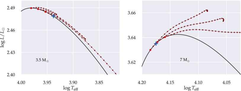
Figure 6: Two examples of comparing secular stability as evidenced in MESA directly as compared with the appearance of an unstable monotonic mode in the linear secular approximation.

The NNE ansatz was invoked at a few selected epochs – in the neighborhood of the blue edge of the monotonic secular-mode instability as computed with the Riccati code (shown as blue crosses in Fig. 6) – for the 3.5 and the 7 $M_{\odot}$ models, respectively. The starting epochs are marked by red dots on the QHE evolutionary track in Fig. 6. A few models along the NNE tracks are plotted as connected smaller dark-red dots. If the starting model is thermally stable, the corresponding NNE track does not significantly drift off the QHE track but quite quickly stalls and the timestep of the computation grows without bound (because nothing happens anymore to the star). If the initial model is thermally unstable, though, its NNE evolution takes it to a new thermally stable configuration which can be far from the initial QHE location on the HR plane. In both panels of Fig. 6, the earlier two starting models along the 3.5 and the 7 $M_{\odot}$ sequences are both thermally stable. The third NNE loci of both sequences diverge from the respective QHE tracks and head towards the FGB far outside the figures. Even though the linear secular analyses do not pin down the onset of the instability very accurately, they remain nonetheless helpfully indicative.

Along the FGB, the situation is less obvious: As mentioned before, the linear secular stability analyses failed to find red edges in any of the computed model sequences. Is this real or a problem of the Riccati code? Once again we ran the NNE experiment, this time along the lower FGB branches.

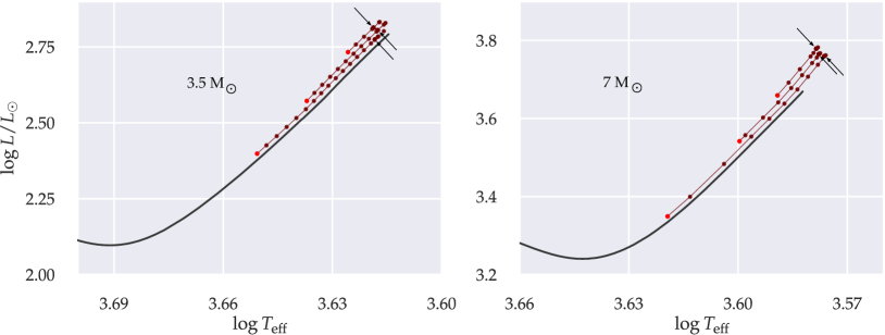
Figure 7: Comparable to Fig. 6 but now in the region of the FGB where the red edge of the unstable monotonic secular mode was expected not found. For clarity, the NNE tracks along the FGB are each shifted by multiples of $0.002$ in $\log T_{\rm eff}$. Without shift all tracks fall essentially onto the QHE FGB locus. Arrows point to the positions of the terminal locations where the NNE tracks stalled.

Figure 7 zooms in to the lower FGBs of the 3.5 (left panel) and the 7 $M_{\odot}$ (right panel) QHE tracks (shown as black lines). The tracks stop at ignition of core He-burning. Superposed on the QHE tracks are, as in Fig. 6, NNE tracks that started at three different epochs (bright red dots) along the FGB. In both panels of Fig. 7 the NNE tracks are successively shifted in $T_{\rm eff}$ to avoid overlapping. All NNE tracks followed very closely the locus of the QHE one. In all cases the NNE models drifted away from their initial QHE position on the HR plane. On a thermal timescale they all evolved up the FGB and all stalled at about the same luminosity. In the 3.5 $M_{\odot}$ case the terminal luminosity as close to that of the QHE epoch where core He-burning ignites. Inspection of central $\rho,T$ of the final NNE models reveals that they too would be ready to start core He-burning. The very definition of NNE though prevents them from changing their nuclear composition. Therefore, NNE evolution must stall along the FGB. The same applies to the 7 $M_{\odot}$ sequence even though in NNE models He-burning ignition conditions are only reached at luminosities that are somewhat higher than those of the QHE models.

If stellar models are thermally unstable – in the NNE sense – depends on the definition of a suitable neighborhood that is to be left upon starting NNE evolution at a chosen QHE epoch. Along the FGB such a neighborhood is particularly ill-defined because it seems constrained by the evolution along the Hayashi track and the suppression of core He-burning. Nonetheless, at the very least the NNE models from the earliest two epochs around the base of the FGB evolve away considerably from their QHE location (in both stellar-mass examples) so that they likely qualify as secularly unstable. If the same applies to the respective last QHE epochs must remain open for the moment.

References

- Aizenman & Perdang (1971a) Aizenman, M. L. & Perdang, J. 1971a, A&A, 12, 232
- Aizenman & Perdang (1971b) —. 1971b, A&A, 15, 200
- Gabriel (1972) Gabriel, M. 1972, A&A, 18, 242
- Gabriel & Ledoux (1967) Gabriel, M. & Ledoux, P. 1967, AnAp, 30, 975
- Gautschy & Althaus (2007) Gautschy, A. & Althaus, L. 2007, A&A, 471, 911
- Hansen (1978) Hansen, C. J. 1978, ARA&A, 16, 15
- Kähler (1972) Kähler, H. 1972, A&A, 20, 105
- Kippenhahn et al. (2012) Kippenhahn, R., Weigert, A., & Weiss, A. 2012, Stellar Structure and Evolution, 2nd ed. (Springer)
- Lauterborn & Siquig (1976) Lauterborn, D. & Siquig, R. 1976, A&A, 49, 285
- Ledoux (1969) Ledoux, P. 1969, in La structure interne des étoiles, XIe cours de perfectionnement de l’association vaudoise des chercheurs en physique, Saas-Fee 1969, 45
- Paczyński (1972) Paczyński, B. 1972, AcA, 22, 163
- Paxton et al. (2013) Paxton, B., Cantiello, M., Arras, P., et al. 2013, ApJS, 208, 4
- Paxton et al. (2018) Paxton, B., Schwab, J., Bauer, E. B., et al. 2018, ApJS, 234, 34
- Phillips (1929) Phillips, T. E. R. 1929, MNRAS, 89, 404
- Roth (1973) Roth, M. 1973, PhD thesis, Universität Hamburg
- Sandage & Schwarzschild (1952) Sandage, A. R. & Schwarzschild, M. 1952, ApJ, 116, 463
- Scuflaire et al. (1995) Scuflaire, R., Noels, A., & Carlier, F. 1995, Liège International Astrophysical Colloquia, No. 32, 423
- Spindler & Lauterborn (1977) Spindler, G. & Lauterborn, D. 1977, A&A, 58, 445
- Strömberg (1932) Strömberg, G. 1932, ApJ, 75, 115