Voronoi diagrams of algebraic varieties under polyhedral norms

Abstract.

We study Voronoi diagrams of manifolds and varieties with respect to polyhedral norms. We provide upper and lower bounds on the dimensions of Voronoi cells. For algebraic varieties, we count their full-dimensional Voronoi cells. As an application, we consider the polyhedral Wasserstein distance between discrete probability distributions.

1. Introduction

Given a metric space $(M,f)$ and a subset $X\subseteq M$, its Voronoi diagram is the collection of Voronoi cells indexed by points of $X$. The cell corresponding to $x\in X$ is given by all points of $M$ which are closer to $x$ than to any other point in $X$. The first appearance of this idea in the sciences can be traced back to the work of Descartes and his interpretation of the solar system as a union of convex regions corresponding to fixed stars. At the beginning of the 20th century, the mathematician Georgy Fedoseevich Voronoi gave a formal definition of the diagrams which now carry his name. Since then, Voronoi diagrams found a long list of applications and specializations in different areas: from electrical engineering, network and data analysis to medicine.

The most popular version of Voronoi diagrams consists of the following choice of ingredients: $M=\mathbb{R}^{n}$, $f$ is the Euclidean distance on $M$, and $X$ is a finite set of points or a lattice. However, our focus is on a different setting:

We let the ambient space $M$ to be an affine space with a a polyhedral distance, i.e., a distance for which the unit balls are convex polytopes. We shall not only consider countable subsets $X$ of points, but higher dimensional manifolds and varieties. This choice produces a Voronoi diagram with an infinite number of cells as these are indexed by points in $X$.

Even though most of our technical results hold true in this general setting, we will focus on the following motivating application. Let us consider the affine hyperplane $\mathbf{1}_{n}:=\{(t_{1},\dots,t_{n+1}):\sum_{i}t_{i}=1\}\subseteq\mathbb{R}^{n+1}$ and the probability simplex $\Delta_{n}:=\mathbf{1}_{n}\cap\mathbb{R}^{n+1}_{\geq 0}$. The latter is the space of discrete probability distributions on $n+1$ states. We consider a Wasserstein distance $W_{d}$ on $\mathbf{1}_{n}$ (or its restriction to $\Delta_{n}$). The distance $W_{d}$ is determined by a metric $d$ on the finite set of states $\{1,\dots,n+1\}$. We can interpret $d$ as describing the cost of transporting a unit of mass from one state to another. Then, the Wasserstein distance $W_{d}(\mu,\nu)$ is the minimal cost of transforming the distribution $\mu$ into the distribution $\nu$ by moving mass between the different states.

In more mathematical terms, $W_{d}(\mu,\nu)$ can be computed by optimizing a linear cost function (determined by $d$ alone) over the convex transportation polytope (determined by $\mu$ and $\nu$). The notion of Wasserstein distance is at the core of the field of optimal transport [Vil08], and gained recently popularity in machine learning, where it has been successfully employed as a loss function for generative adversarial networks (WGANs) [ACB17, FZM⁺15]. For us, the key observation in the setting of discrete probability distributions is that Wasserstein unit balls are convex polytopes, known in the literature as Kantorovich-Rubinstein or fundamental polytopes [Ver15, GP17].

Many statistical applications deal with the problem of determining which distribution in a given statistical model $X\subsetneq\Delta_{n}$ best explains some observed data. That problem can typically be phrased as finding a distribution in $X$ that is closest to an observed distribution. In [ÇJM⁺20, ÇJM⁺21], the authors study the problem of describing and computing the Wasserstein distance to a model $X$ that is an algebraic variety, i.e., the zero locus of a finite set of polynomials. This assumption is satisfied by a wide variety of models in statistics, such as models of independence and discrete exponential families. Our study can be seen as a reformulation of the question above:

Given a point $x$ in a statistical model $X$, what is the set of empirical distributions that are better explained, in the sense of Wasserstein distance, by $x$ than by any other point in the model?

In [CRSW20], the authors study a similar question, when the distance is the Euclidean one. They prove that the Euclidean Voronoi cell at a smooth point $x\in X$ is convex, and contained in the normal space of $X$ at $x$. Moreover, this cell is full-dimensional in the normal space. If the point $x$ is singular, then the corresponding Voronoi cell can be full-dimensional in the ambient space of $X$. In contrast, when using Wasserstein distances, we observe that full-dimensional cells can occur even at smooth points. This is due to the geoemetric difference between the corresponding unit balls: while the boundary of the Euclidean unit ball is smooth, a convex polytope has only a piecewise smooth boundary. Other related works study the special case of plane curves [BW19], Voronoi cells arising from maximum likelihood estimation [AH21, AH22], and Voronoi diagrams of points in the context of tropical geometry [CJ⁺21]. The distance considered in [CJ⁺21] corresponds to a Wasserstein distance (for a specific choice of $d$) via Kantorovich-Rubinstein duality.

After the necessary preliminaries and definitions in Section 2, we study the dimensions of Voronoi cells depending on the geometry of the set $X$ in Section 3. We consider a specific example Section 4: We compute the number of full-dimensional Voronoi cells of the Hardy-Weinberg curve in $\Delta_{2}$ with respect to every Wasserstein distance. Finally, in Section 5, we provide an upper bound for the number of full-dimensional Voronoi cells when the set $X$ is an algebraic variety. Although for a general polyhedral distance this bound depends also on the combinatorics of the unit ball, in the case of Wasserstein distances it can be relaxed and made dependent only on the dimension of the ambient space and on the geometry of the variety.

2. Polyhedral norms and Wasserstein distances

Let $\mathbb{A}^{n}$ denote a real affine $n$-dimensional space. We will consider affine $n$-dimensional spaces embedded in $\mathbb{R}^{n+1}$. For a metric $D$ on $\mathbb{A}^{n}$, we consider the closed $D$-balls $B_{D,r}(c):=\{x\in\mathbb{A}^{n}\,:\,D(x,c)\leq r\}$ with center $c\in\mathbb{A}^{n}$ and radius $r\geq 0$. If the center and radius of a closed ball are not relevant, we simply write $B_{D}$.

Definition 2.1.

The metric $D$ is a polyhedral distance if it is translation invariant and the $D$-balls $B_{D,r}(c)$ of positive radius are convex $n$-dimensional polytopes.

We note that the polytopes $B_{D,r}(c)$ associated with a polyhedral distance are centrally symmetric. Hence, each face $F$ of the polytope $B_{D,r}(c)$ has an opposite face, which we denote by $-F$. Basic examples of polyhedral distances are those induced by the $L_{1}$- and the $L_{\infty}$-norm on $\mathbb{R}^{n}$.

Another large family of polyhedral distances is given by Wasserstein distances, defined on $\mathbf{1}_{n}$. Let $d$ be a metric on the finite set $[n+1]:=\{1,\dots,n+1\}$. We can naturally identify $d$ with a symmetric matrix $d=(d_{ij})\in\mathbb{R}_{\geq 0}^{(n+1)\times(n+1)}$ that satisfies the triangular inequalities $d_{ij}\leq d_{ik}+d_{kj}$ for every $1\leq i,j,k\leq n+1$. Given $\mu,\nu\in\mathbf{1}_{n}$, the transportation polytope from $\mu$ to $\nu$ is

$$\Pi(\mu,\nu):=\left\{y\in\mathbb{R}_{\geq 0}^{(n+1)\times(n+1)}\;:\;\forall\,1\leq i,j\leq n+1,\;\sum_{k=1}^{n+1}y_{ik}=\mu_{i}\text{ and }\sum_{k=1}^{n+1}y_{kj}=\nu_{j}\right\}.$$

Definition 2.2.

The Wasserstein distance $W_{d}(\mu,\nu)$ of $\mu$ and $\nu$ associated with $d$ is the solution to the following linear optimization problem:

$$\text{minimize}\sum_{i,j=1}^{n+1}d_{ij}x_{ij}$$

$$\text{subject to }x=(x_{ij})\in\Pi(\mu,\nu).$$

If we interpret $\mu$ and $\nu$ as mass distributions, $x$ can be thought of as a transportation plan, in which the entry $x_{ij}$ indicates the amount of mass that is transported from $\mu_{i}$ to $\nu_{j}$ in order to transform one distribution into the other. The matrix $d$ determines the cost of each transportation step.

The Wasserstein balls (i.e., the closed $W_{d}$-balls associated with a Wasserstein distance $W_{d}$ on $\bm{1}_{n}$) can be expressed as a convex hull of $2\binom{n+1}{2}$ points:

$$B_{W_{d},r}(c)=\text{conv}\left\{c+r\frac{e_{i}-e_{j}}{d_{ij}}\leavevmode\nobreak\ :\leavevmode\nobreak\ \leavevmode\nobreak\ i,j\in[n+1],i\neq j\right\},$$

where $e_{i}$ denotes the $i$-th vector of the standard basis of $\mathbb{R}^{n+1}$. Note that those $2\binom{n+1}{2}$ points do not need to be in convex position, as the following example demonstrates.

Example 2.3.

Figure 1 shows the Wasserstein balls of radius $r=\frac{1}{3}$ and center $c=(\frac{1}{3},\frac{1}{3},\frac{1}{3})$ associated with the distances

$$d_{1}=\begin{pmatrix}0&1&1\\ 1&0&1\\ 1&1&0\end{pmatrix}\quad\text{and}\quad d_{2}=\begin{pmatrix}0&1&2\\ 1&0&1\\ 2&1&0\end{pmatrix}.$$

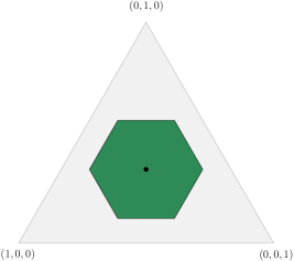
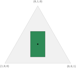
Figure 1. Wasserstein balls $B_{W_{d_{1}},\frac{1}{3}}(\frac{1}{3},\frac{1}{3},\frac{1}{3})$ and $B_{W_{d_{2}},\frac{1}{3}}(\frac{1}{3},\frac{1}{3},\frac{1}{3})$.

These are all cases for the possible number of sides of Wasserstein balls in the plane $\mathbf{1}_{2}$. Indeed, planar Wasserstein balls are the convex hulls of six points. As centrally symmetric polytopes have an even number of vertices, that number must be either four or six.

3. Dimensions of Voronoi cells

Our main object of study is the Voronoi decomposition of a set $X$ under a polyhedral distance. We are particularly interested in the case of an algebraic variety $X$ under a Wasserstein distance. This section is devoted to finding lower and upper bounds on the dimensions of the Voronoi cells.

Definition 3.1.

Let $(M,f)$ be a metric space and $X\subseteq M$ be a set. The (open) Voronoi cell $V_{f,X}(x)$ of a point $x\in X$ is the set

$$V_{f,X}(x)=\{y\in M\leavevmode\nobreak\ :\leavevmode\nobreak\ \forall x^{\prime}\in X\setminus\{x\},f(x,y)<f(x^{\prime},y)\}.$$

From now on we fix a polyhedral distance $f=D$ on real affine $n$-space $M=\mathbb{A}^{n}$. An important tool in our analysis are the face cones of the closed $D$-balls $B_{D,r}(c)$. The face cone of a face $F$ is the cone over the opposite face $-F$. For the formal definition, we denote by $\mathrm{int}(\cdot)$ the relative interior.

Definition 3.2.

Let $F$ be a non-empty face of the polytope $B_{D,r}(x)$ for some $x\in\mathbf{1}_{n}$ and $r\geq 0$. The face cone of $F$ at $x$ is the set

$$C_{F}(x):=\{x+\delta(s-x)\;:\;s\in\mathrm{int}(-F),\delta>0\}.$$

We set $C_{\emptyset}(x)=\{x\}$. We also define the truncated face cone for some $\varepsilon>0$ as follows:

$$C_{F,\varepsilon}(x)=\{x+\delta(s-x)\;:\;s\in\mathrm{int}(-F),\varepsilon>\delta>0\}.$$

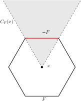
Figure 2. Illustration of the face cone as in Definition 3.2.

The face cone of a face $F$ at a point $x$ is the set of all points such that the $D$-ball of some (positive) radius around these points intersects $x$ at $F$; see Figure 2. We note that the definition of the face cone $C_{F}(x)$ does not depend on the radius $r$ of the ball $B_{D,r}(x)$ while the truncated face cone $C_{F,\varepsilon}(x)$ does. Moreover, we observe that $C_{F,\varepsilon}(x)\subseteq B_{D,\varepsilon}(x).$ Most notably, the face cones of the distinct faces of a $D$-ball centered at $x$ partition the Voronoi cell $V_{D,X}(x)$ of $x$, i.e.,

$$V_{D,X}(x)=\underset{F\subsetneq B_{D,r}(x)\text{ face}}{\dot{\bigcup}}\left(V_{D,X}(x)\cap C_{F}(x)\right).$$ (1)

We make use of this in a first dimension estimate of Voronoi cells.

Proposition 3.3.

Let $X\subseteq\mathbb{A}^{n}$ be a subset and let $x\in X$ be a point. Assume that $y\in V_{D,X}(x)$ with $y\neq x$, and let $\varepsilon>0$ be the radius such that $\partial B_{D,\varepsilon}(y)\cap X=\{x\}$. Let $F$ be the unique face of $B_{D,\varepsilon}(y)$ whose relative interior contains $x$. Then $\dim V_{D,X}(x)\geq\dim F+1.$

Proof.

We claim that $C_{-F,\varepsilon}(y)\cap C_{F}(x)\subseteq V_{D,X}(x)$. Let $z$ be a point in the intersection. Since both $x\in C_{-F}(y)$ and $z\in C_{-F,\varepsilon}(y)\cap C_{F}(x)$, the polyhedral distances $D(x,y)$, $D(x,z)$ and $D(y,z)$ are measured evaluating the same linear functional. In particular, it holds that $D(x,y)=D(x,z)+D(y,z)$. Assume now that there exists a point $x^{\prime}\in X$ with $D(x^{\prime},z)\leq D(x,z)$. Then by the triangular inequality we obtain that

$$D(x^{\prime},y) \leq D(x^{\prime},z)+D(y,z)$$

$$\leq D(x,z)+D(x,y)-D(x,z)=D(x,y),$$

which contradicts the fact that $y\in V_{D,X}(x)$.

Since the relative interior of the line segment from $x$ to $y$ lies in both $C_{-F,\varepsilon}(y)$ and $C_{F}(x)$, their intersection is nonempty. Moreover, inside the $(\dim F+1)$-dimensional affine space spanned by $F$ and $y$, both $C_{-F,\varepsilon}(y)$ and $C_{F}(x)$ are full-dimensional and open, and so is their intersection. Hence, the dimension of the Voronoi cell $V_{D,X}(x)$ is at least $\dim F+1$. ∎

The lower bound in Proposition 3.3 depends on finding a point in the Voronoi cell $V_{D,X}(x)$. We now give another lower bound that only depends on the faces of the $D$-balls.

We do this by splitting an open neighbourhood around $x$ with a hyperplane that leaves $X$ entirely on one side. For this, we consider a Euclidean ball in $\mathbb{R}^{n+1}$ centered at a point $x\in\mathbb{A}^{n}$ of radius $r$ and denote with $\beta_{r}(x)$ its restriction to $\mathbb{A}^{n}$.

For a proper face $F$ of a $D$-ball, we define a family of parallel hyperplanes in $\mathbb{A}^{n}$ as follows: Let the $D$-ball be centered at $c\in\mathbb{A}^{n}$. We denote by $v_{F}$ the outer orthonormal vector to the face $F-c=\{p-c\leavevmode\nobreak\ :\leavevmode\nobreak\ p\in F\}$ in the linear space $\text{span}((F-c)\cup\{\mathbf{0}\})$. Here the inner product that defines $v_{F}$ is the one induced by the standard inner product on $\mathbb{R}^{n+1}$, in which $\mathbb{A}^{n}$ is embedded. We write $H_{F}$ for the hyperplane in the linear space $\mathbb{A}^{n}-c$ that is the orthogonal complement of $v_{F}$. Finally, for any point $x\in\mathbb{A}^{n}$, we define $H_{F,x}:=H_{F}+x$ for the hyperplane in $\mathbb{A}^{n}$ that passes through $x$. If $\dim F=k$, then we call $H_{F,x}$ a $k$-face hyperplane through $x$. Note that the definition of $H_{F,x}$ does not depend on the center $c$, and that $H_{F,x}=H_{-F,x}$

Proposition 3.4.

Let $X\subseteq\mathbb{A}^{n}$ be a subset and $x\in X$ be a point. If there exists a radius $r>0$ and a $k$-face hyperplane through $x$ that bisects the Euclidean ball $\beta_{r}(x)$ in such a way that the closure of one of the resulting half-balls intersects $X$ only at $x$, then $\dim V_{D,X}(x)\geq k+1.$

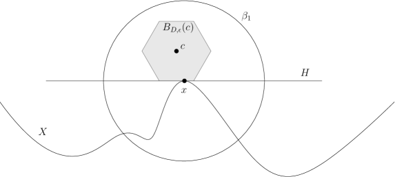
Figure 3. Example illustration of setup in proof of Proposition 3.4 in the plane.

Proof.

We denote with $H$ the $k$-face hyperplane that bisects $\beta_{r}(x)$ into two closed half-balls, say $\beta_{1}$ and $\beta_{2}$. Without loss of generality, $\beta_{1}\cap X=\{x\}$. We choose a point $c\in\beta_{1}$ and a sufficiently small $\varepsilon>0$ such that the following two conditions hold: 1) $B_{D,\varepsilon}(c)\subseteq\beta_{1}$ and 2) $x$ is in the relative interior of a $k$-face $F$ of $B_{D,\varepsilon}(c)$ with $H=H_{F,x}$; see Figure 3. In particular, this gives us a point $c$ in the Voronoi cell of $x$ such that $\partial B_{D,\varepsilon}(c)\cap X=\{x\}$. By Proposition 3.3, $V_{D,X}(x)$ has dimension at least $k+1.$ ∎

We now aim to find upper bounds for the dimension of a Voronoi cell. For this, we will determine which faces do not appear in the decomposition (1) of a given Voronoi cell. We restrict our investigation to sets $X$ that are algebraic varieties, but note that the statements in this section also apply to manifolds. Similarily to the construction of the $k$-face hyperplanes $H_{F,x}$, we define for every face $F$ of a $D$-ball and for every point $x\in\mathbb{A}^{n}$ the affine face space $A_{F,x}$ to be the affine hull $\mathrm{span}(F)$ translated such that it passes through $x$.

Lemma 3.5.

Let $X\subsetneq\mathbb{A}^{n}$ be an algebraic variety and $x\in X$ be a smooth point. If an affine face space $A_{F,x}\subsetneq\mathbb{A}^{n}$ through $x$ intersects $X$ at $x$ transversally, then the Voronoi cell $V_{D,X}(x)$ does not contain any point in the face cone $C_{F}(x)$.

Proof.

We assume for contradiction that there exists a point $y\in V_{D,X}(x)\cap C_{F}(x).$ This means that $\partial B_{D,\varepsilon}(y)\cap X=\{x\}$ for some $\varepsilon>0$ and that $F$ is the unique face of $B_{D,\varepsilon}(y)$ whose relative interior contains $x$.

We now restrict our problem to the affine span of $A_{F,x}$ and $y$, denoted by $\mathbb{A}$. Inside $\mathbb{A}$, the affine space $A_{F,x}$ is a hyperplane that intersects $X^{\prime}:=X\cap\mathbb{A}$ at $x$ transversally. Note that $x$ is non-singular on $X^{\prime}$. Moreover, since $x$ is the closest point to $y$, it is a local minimum for the linear functional defined by the vector $v_{F}$ orthogonal to $A_{F,x}$. However, this yields a contradiction since smooth critical points of the problem of optimizing a linear functional $\langle v_{F},\cdot\rangle$ over an algebraic variety are precisely the points for which the tangent space is parallel to the orthogonal complement of $v_{F}$.

∎

By applying Lemma 3.5 to all faces of large dimension, we obtain an upper bound on the dimension of a Voronoi cell.

Theorem 3.6.

Let $X\subsetneq\mathbb{A}^{n}$ be an algebraic variety and $x\in X$ be a smooth point. If an affine face space $A_{F,x}$ through $x$ intersects $X$ at $x$ non-transversally and no affine face space of larger dimension has this property, then the Voronoi cell $V_{D,X}(x)$ is of dimension at most $\dim F+1$.

Proof.

For any face $F^{\prime}$ with $\dim F^{\prime}>\dim F$, we have that $V_{D,X}(x)\cap C_{F}(x)=\emptyset$ by Lemma 3.5. Recall that we can partition the Voronoi cell as in (1). Hence, we conclude that $\dim V_{D,X}(x)\leq\dim C_{F}(x)=\dim F+1$. ∎

A first application of Theorem 3.6 is to detect all full-dimensional cells at smooth points in the Voronoi diagram of a variety $X$. For this, we note that for a facet $F$, the affine face space $A_{F,x}$ equals the facet hyperplane $H_{F,x}$.

Corollary 3.7.

Let $x$ be a smooth point on an algebraic variety $X\subsetneq\mathbb{A}^{n}$. If the Voronoi cell $V_{D,X}(x)$ is full-dimensional, then one of the facet hyperplanes through $x$ is tangent to $X$ at $x$.

Proof.

By Theorem 3.6, for a Voronoi cell of dimension $n$, there has to be a face $F$ with $n\leq\dim F+1$ (i.e., a facet) such that the hyperplane $A_{F,x}=H_{F,x}$ is tangent to $X$ at $x$. ∎

In general, the tangency of a facet hyperplane is only a necessary – and not a sufficient – condition for the full-dimensionality of a Voronoi cell. However, we can reverse Corollary 3.7 in the following sense: Once a hyperplane spanned by a facet $F$ is tangent, the assumptions in Propositions 3.3 and 3.4 become equivalent conditions to that the facet $F$ contributes a full-dimensional part of the Voronoi cell.

Corollary 3.8.

Let $x$ be a smooth point on an algebraic variety $X\subsetneq\mathbb{A}^{n}$ such that the facet hyperplane $H_{F,x}$ is tangent to $X$ at $x$. Then the following are equivalent:

• $V_{D,X}(x)\cap C_{F}(x)\neq\emptyset$ or $V_{D,X}(x)\cap C_{-F}(x)\neq\emptyset$ (which implies that the Voronoi cell is full-dimensional).

• There exists $y\in V_{D,X}(x)$ and $\varepsilon>0$ such that $\partial B_{D,\varepsilon}(y)\cap X=\{x\}$ and $x$ is contained in the relative interior of a facet $F^{\prime}$ of $B_{D,\varepsilon}(y)$, with $H_{F^{\prime},x}=H_{F,x}$ (cf. Proposition 3.3).

• There exists $r>0$ such that all the points in $X\setminus\{x\}\cap\beta_{r}(x)$ lie in one open half ball obtained by bisecting the Euclidean ball $\beta_{r}(x)$ with $H_{F,x}$ (cf. Proposition 3.4).

Proof.

In the proof of Proposition 3.3, we show that the intersection of the Voronoi cell with the face cone $C_{F^{\prime}}(x)$ is non-empty, which gives us the implication $(b)$$\Rightarrow$$(a)$. Similarly, the proof of Proposition 3.4 yields $(c)$$\Rightarrow$$(a)$.

To show $(a)$$\Rightarrow$$(b)$, consider any point $y\in V_{D,X}(x)\cap C_{F}(x)$. Since $y$ is in the face cone of $F$, the facet $F$ of some $D$-ball centered at $y$ contains $x$ in its relative interior. Moreover, since $y$ is also in the Voronoi cell, the boundary of that ball intersects $X$ only at $x$.

To see $(b)$$\Rightarrow$$(c)$, we choose a Euclidean ball $\beta_{r}(x)$ small enough so that its intersection with $H_{F,x}$ is contained in $F$. Furthermore, we can choose it small enough such that one of its open half balls is contained in $B_{D,\varepsilon}(y)$. Since $\partial B_{D,\varepsilon}(y)\cap X=\{x\}$ and $y\in V_{D,X}(x)$, that half ball does not intersect $X$. Hence, all points in $X\setminus\{x\}\cap\beta_{r}(x)$ lie in the other half ball. ∎

Remark 3.9.

For arbitrary (lower-dimensional) faces, a weaker version of Corollary 3.8 holds. Let us consider a smooth point $x$ on a variety $X$ and an affine face space $A_{F,x}$ of maximal dimension such that it intersects $X$ at $x$ non-transversally. Recall that $\dim V_{D,X}(x)\leq\dim F+1$ by Theorem 3.6. In this setting, the conditions $(a)$ and $(b)$ in Corollary 3.8 are still equivalent, after replacing “full-dimensional” in $(a)$ with “$(\dim F+1)$-dimensional” as well as “facet” and “$H_{F^{\prime},x}=H_{F,x}$” in $(b)$ with “face” resp. “$A_{F^{\prime},x}=A_{F,x}$”. This can be seen with the same proofs as above. Similarly, $(c)$ still implies $(a)$ and $(b)$. However, the reverse implication is generally not true. A simple counterexample is a plane curve $X$ with a smooth point $x$ of inflection and an appropriately chosen $D$-ball with vertex $F$.

4. Wasserstein-Voronoi cells for the Hardy-Weinberg curve

We now turn our attention to a concrete example. We examine full-dimensional Voronoi cells for the planar Hardy-Weinberg curve under varying Wasserstein distances. We show that any Wasserstein-Voronoi diagram of that curve has one, two, or three full-dimensional Voronoi cells. The Hardy-Weinberg curve is the set of distributions we find by recording the total number of “heads” obtained from tossing a biased coin twice. It is parametrized by the bias of the coin, i.e., the probability of the outcome of a single experiment being “head”. Tossing the coin more than twice, we obtain the Veronese curves that are parametrized by

$$\varphi_{n}\leavevmode\nobreak\ :\leavevmode\nobreak\ [0,1]\to\Delta_{n},$$

$$p\mapsto\left(p^{n},np^{n-1}(1-p),\binom{n}{2}p^{n-2}(1-p)^{2},\dots,\binom{n}{n-1}p(1-p)^{n-1},\binom{n}{n}(1-p)^{n}\right),$$ (2)

where $\Delta_{n}=\{(t_{0},\cdots,t_{n})\in\mathbb{R}^{n+1}_{\geq 0}\leavevmode\nobreak\ :\leavevmode\nobreak\ t_{0}+\cdots+t_{n}=1\}.$

In order to detect all full-dimensional Voronoi cells of the Hardy-Weinberg curve $\varphi_{2}([0,1])$, we make use of Corollary 3.7 which requires us to find all facet hyperplanes (in our case, edge lines) of a given Wasserstein ball that are tangent to the curve. Recall that planar Wasserstein balls have at most six edges (see Example 2.3).

Lemma 4.1.

Let $d=\begin{pmatrix}0&d_{12}&d_{13}\\ d_{12}&0&d_{23}\\ d_{13}&d_{23}&0\end{pmatrix}$. Each of the three directional vectors of the edges of the Wasserstein ball of $d$ is tangent at at most one interior point of the Hardy-Weinberg curve (i.e., to $\varphi_{2}((0,1))$). Tangency occurs under the following conditions:

• The vector $\dfrac{e_{1}-e_{2}}{d_{12}}-\dfrac{e_{1}-e_{3}}{d_{13}}$ is tangent if and only if $d_{12}>d_{13}$.

• The vector $\dfrac{e_{1}-e_{3}}{d_{13}}-\dfrac{e_{2}-e_{3}}{d_{23}}$ is tangent if and only if $d_{23}>d_{13}$.

• The vector $\dfrac{e_{1}-e_{2}}{d_{12}}-\dfrac{e_{3}-e_{2}}{d_{23}}$ is tangent for any $d$.

Proof.

The tangent vector at the point $\varphi_{2}(p)$ of the curve is parametrized by

$$\left(2p,\,2-4p,\,2p-2\right).$$ (3)

We start by considering the edge with directional vector as in $(a)$. The points $\varphi_{2}(p^{*})$ of the curve whose tangent vector is parallel to the edge are the solutions of the system

$$(2p,\,2-4p,\,2p-2)=\lambda(d_{12}-d_{13},\,d_{13},\,-d_{12}),$$

for some $\lambda\neq 0$, from which we obtain

$$p^{*}=\dfrac{d_{12}-d_{13}}{2d_{12}-d_{13}}.$$

In particular, $p^{*}\in(0,1)$ if and only if $d_{12}>d_{13}$. Statement $(b)$ follows by symmetry, as the Hardy-Weinberg curve is invariant under permutation of the first and the third coordinate.

For the edge specified in $(c)$, the points $\varphi_{2}(p^{*})$ of the curve whose tangent vector is parallel are the solutions of the system

$$(2p,2-4p,2p-2)=\lambda(d_{23},d_{12}-d_{23},-d_{12})$$

for some $\lambda\neq 0$, from which we obtain

$$p^{*}=\dfrac{d_{23}}{d_{12}+d_{23}}.$$

Since $d_{ij}>0$, we see that $p^{*}\in(0,1)$. ∎

We now divide the space $(d_{12},d_{13},d_{23})$ of metrics on $[3]=\{1,2,3\}$ according to the number of full-dimensional Voronoi cells of the Hardy-Weinberg curve.

Theorem 4.2.

The number of full-dimensional Voronoi cells of a Wasserstein-Voronoi diagram of the Hardy-Weinberg curve in the simplex $\Delta_{2}$ is

$$\begin{cases}1&\text{if }d_{13}>\max\{d_{12},d_{23}\}\\ 2&\text{if }d_{12}<d_{13}<d_{23}\text{ or }d_{23}<d_{13}<d_{12}\\ 3&\text{if }d_{13}<\min\{d_{12},d_{23}\}\end{cases}.$$

Proof.

We know from Corollary 3.7 that full-dimensional Voronoi cells can only appear if the tangent line of a point on the curve is the affine hull of an edge of the Wasserstein ball. Since the Hardy-Weinberg curve is a smooth conic, it lies in one of the half-planes bisected by the tangent line at any point. Hence, by Corollary 3.8$(c)$, there is a full-dimensional Voronoi cell at a point if and only if its tangent vector is parallel to an edge. Lemma 4.1 provides linear conditions describing this tangency for each of the edge directions. The statement follows combining those conditions. ∎

We note that all three cases in Theorem 4.2 can occur for hexagonal Wasserstein balls (i.e., not just for degenerate balls with four edges), as the following example demonstrates.

Example 4.3.

Under the three Wasserstein distances associated with the metrics

$$d_{1}=\begin{pmatrix}0&1&1\\ 1&0&1\\ 1&1&0\end{pmatrix},\quad d_{2}=\begin{pmatrix}0&2&3\\ 2&0&4\\ 3&4&0\end{pmatrix},\quad\text{ and }d_{3}=\begin{pmatrix}0&2&1\\ 2&0&2\\ 1&2&0\end{pmatrix},$$

the Hardy-Weinberg curve has one, two, or three full-dimensional Voronoi cells, respectively. This can be seen immediately from Theorem 4.2. Following the calculations in the proof of Lemma 4.1, we can find the full-dimensional Voronoi cells at the points $p=\dfrac{1}{2}$, $p\in\{\dfrac{2}{3},\dfrac{4}{5}\}$, and $p\in\{\dfrac{1}{3},\dfrac{1}{2},\dfrac{2}{3}\}$, respectively; see Figure 4.

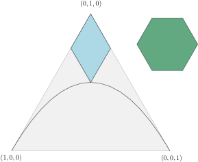
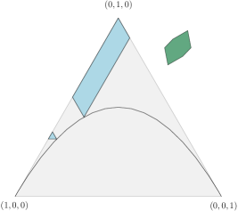
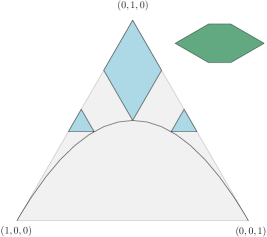
Figure 4. Full-dimensional Voronoi cells of the Hardy-Weinberg curve under the Wasserstein distances $W_{d_{1}}$ (top left), $W_{d_{2}}$ (top right), and $W_{d_{3}}$ (bottom row) from Example 4.3. The respective Wasserstein balls are depicted in green.

In the toy example of the Hardy-Weinberg curve, Theorem 4.2 gives a complete understanding of the space of Wasserstein metrics in terms of the number of full-dimensional Voronoi cells. A result of this form would be desirable for any family of statistical models. We propose the following problem.

Problem 4.4.

Let $C_{n}=\varphi_{n}([0,1])\subseteq\Delta_{n}$ be the Veronese curve parametrized as in (4). Find a decomposition of the space of metrics on $[n+1]$ such that the metrics in every region yield Wasserstein-Voronoi diagrams with the same number of full-dimensional cells.

5. Counting full-dimensional cells

In this section, we find an upper bound for the number of full-dimensional Voronoi cells of smooth irreducible varieties under a polyhedral distance $D$ on $\mathbb{A}^{n}$. Our main tool is projective duality. Hence, even though we are interested in real affine varieties $X\subseteq\mathbb{A}^{n}$, we pass to their complex projective closure $\overline{X}\subseteq\mathbb{P}^{n}$. We denote by $(\mathbb{P}^{n})^{*}$ the dual projective space, i.e., the set of hyperplanes of $\mathbb{P}^{n}$. For a subvariety $\overline{X}\subseteq\mathbb{P}^{n}$, we consider the set of all hyperplanes that are tangent to $\overline{X}$ at some smooth point. The dual variety $\overline{X}^{\vee}\subseteq(\mathbb{P}^{n})^{*}$ of $X$ is the Zariski closure of that set inside $(\mathbb{P}^{n})^{*}$.

To state the main theorem of this section, we also introduce the notation $F(P)$ for the number of facets of a polytope $P\subseteq\mathbb{A}^{n}$.

Theorem 5.1.

Let $X\subseteq\mathbb{A}^{n}$ be a smooth irreducible variety such that the dual variety $\overline{X}^{\vee}$ of its complex projective closure $\overline{X}$ is a hypersurface in $(\mathbb{P}^{n})^{*}$. The number of full-dimensional Voronoi cells of $X$ under a polyhedral distance $D$ is at most

$$\frac{F(B_{D})\,\deg(\overline{X}^{\vee})}{2}.$$ (4)

Before we give a proof for Theorem 5.1, we investigate its assumption that the dual variety is a hypersurface. We show now that there are no full-dimensional Voronoi cells without this assumption. Thus, Theorem 5.1 captures all smooth varieties will full-dimensional cells in its Voronoi diagram.

Theorem 5.2.

Let $X\subseteq\mathbb{A}^{n}$ be an irreducible variety and $D$ be a polyhedral distance on $\mathbb{A}^{n}$. If the dual variety $\overline{X}^{\vee}$ of the complex projective closure $\overline{X}$ is not a hypersurface in $(\mathbb{P}^{n})^{*}$, no smooth point $x\in X$ has a full-dimensional Voronoi cell with respect to $D$.

Proof.

Since the dual variety has codimension larger than one (say, codimension $c+1$), the complex projective variety $\overline{X}$ is ruled (by projective spaces of dimension $c$); in other words, $\overline{X}$ is the union of ($c$-dimensional) projective spaces [GKZ94, Chapter 1, Corollary 1.2]. Moreover, the real part of $\overline{X}$, including $X$, is ruled by real spaces of positive dimension. Indeed, for a (generic) real point $p\in\overline{X}$, we consider a real hyperplane tangent at $p$. That hyperplane corresponds to a real point $q\in\overline{X}^{\vee}$. Since the dual variety is not a hypersurface, there is a positive-dimensional family of real hyperplanes tangent at $q$. These hyperplanes correspond to real points on $\overline{X}$ where they form a positive-dimensional projective space passing through $p$.

Now let us assume for contradiction that there is a smooth point $x\in X$ with a full-dimensional Voronoi cell. For any point $y$ in the Voronoi cell, there is a $D$-ball $B_{D,\varepsilon}(y)$ that intersects $X$ exactly at $x$. By Corollaries 3.7 and 3.8, $y$ can be chosen such that $x$ is contained in the relative interior of some facet $F$ of the ball $B_{D,\varepsilon}(y)$ and such that $F$ is tangent to $X$ at $x$. Since $X$ is ruled by real affine spaces of positive dimension, the tangent space of $X$ at $x$ contains such an affine space passing through $x$. In particular, the relative interior of the tangent facet $F$ contains infinitely many points on $X$, which contradicts that $B_{D,\varepsilon}(y)\cap X=\{x\}$. ∎

The proof of Theorem 5.1 for a generic polyhedral distance (i.e., such that the facet hyperplanes of $B_{D}$ are sufficiently generic given the variety $X$) is relatively straightforward (as well will see below). To address arbitrary polyhedral distances, we need the following basic lemma from projective geometry.

Lemma 5.3.

Let $n\geq 2$, let $L\subseteq\mathbb{P}^{n}$ be a projective subspace of codimension two, and let $C\subseteq\mathbb{P}^{n}$ be an irreducible curve. If all tangent lines of $C$ intersect $L$, the curve $C$ is contained in one of the hyperplanes containing $L$.

Proof.

We consider the projection $\pi:\mathbb{P}^{n}\dashrightarrow\mathbb{P}^{2}$ from a generic subspace $P$ of $L$ with codimension one. The Zariski closure $C_{2}$ of $\pi(C)$ is either a point or a plane curve whose tangent lines all pass through the point $\pi(L)$. In either case, the dual variety $C_{2}^{\vee}\subseteq(\mathbb{P}^{2})^{*}$ is contained in a line. Hence, $C_{2}$ itself must be either a point or a line that passes through $\pi(L)$. In particular, the preimage $\pi^{-1}(C_{2})$ is a projective subspace of $\mathbb{P}^{n}$ that is contained in a hyperplane passing through $L$. Now the assertion follows from the inclusion $C\subseteq\pi^{-1}(C_{2})$. ∎

Now we are ready to prove the main theorem of this section.

Proof of Theorem 5.1.

If $n=1$, the only variety $X$ satisfying the assumptions is a single point. Moreover, the only one-dimensional polytopes are line segments, so $F(B_{D})=2$. This proves the assertion in dimension one, and we assume $n\geq 2$ in the following.

We write $k:=\dfrac{F(B_{D})}{2}$ for the number of pairs of opposite facets of the $D$-balls $B_{D}$, and enumerate the facet pairs $\left((F_{1},-F_{1}),(F_{2},-F_{2}),\ldots,(F_{k},-F_{k})\right)$. For each pair $(F_{i},-F_{i})$ of opposite facets, we consider its one-dimensional family of parallel hyperplanes. In the projective space $\mathbb{P}^{n}$, that is a family of hyperplanes that contain a projective subspace $L_{i}\subseteq\mathbb{P}^{n}$ of codimension two that lies at infinity. In the dual projective space $(\mathbb{P}^{n})^{*}$, the family corresponds to the line $L_{i}^{\vee}$. We slightly abuse notation and write $H\in L_{i}^{\vee}$ for a hyperplane $H\subseteq\mathbb{P}^{n}$ containing $L_{i}$.

By Corollary 3.7, if the Voronoi cell of $x\in X$ is full-dimensional, then a hyperplane $H\in L_{i}^{\vee}$ (for some $1\leq i\leq k$) contains the tangent space $\mathbb{T}_{x}\overline{X}\subseteq\mathbb{P}^{n}$ of $\overline{X}$ at $x$. We now investigate all such occurrences of tangency:

$$\mathcal{N}_{i}:=\left\{(x,H)\in\overline{X}\times(\mathbb{P}^{n})^{*}\;:\;\mathbb{T}_{x}\overline{X}\subseteq H,\,H\in L_{i}^{\vee}\right\}.$$

The set $\mathcal{N}_{i}$ is the intersection of the conormal variety $\mathcal{N}_{\overline{X},\overline{X}^{\vee}}:=\{(x,H)\in\overline{X}\times(\mathbb{P}^{n})^{*}:\mathbb{T}_{x}\overline{X}\subseteq H\}$ with the line $L_{i}^{\vee}\subseteq(\mathbb{P}^{n})^{*}$ (more formally, with $\mathbb{P}^{n}\times L_{i}^{\vee}$). Note that the dual hypersurface $\overline{X}^{\vee}$ is the image of the projection of the conormal variety onto the second factor. Hence, if the line $L_{i}^{\vee}$ was generic, then the set $\mathcal{N}_{i}$ would be finite of cardinality $\deg\overline{X}^{\vee}$. Thus, for a sufficiently generic polyhedral distance $D$, we would be done, since Corollary 3.7 implies that the number of full-dimensional Voronoi cells is at most $\sum_{i=1}^{k}|\mathcal{N}_{i}|=k\cdot\deg\overline{X}^{\vee}$.

For an arbitrary polyhedral distance $D$, the varieties $\mathcal{N}_{i}$ might be infinite. We write $\mathcal{N}_{i}=\mathcal{Z}_{i}\cup\mathcal{N}^{\prime}_{i}$, where $\mathcal{Z}_{i}$ is the positive-dimensional components of $\mathcal{N}_{i}$ and $\mathcal{N}^{\prime}_{i}$ contains the remaining points of $\mathcal{N}_{i}$. If $\mathcal{Z}_{i}$ is empty, then $\mathcal{N}_{i}=\mathcal{N}^{\prime}_{i}$ contains $\deg\overline{X}^{\vee}$ many points, counted with multiplicity. Otherwise, there are less than $\deg\overline{X}^{\vee}$ many points in $\mathcal{N}^{\prime}_{i}$. The latter was shown for the intersection of a subvariety of $\mathbb{P}^{m}$ with a subspace of complementary dimension in [JKW21, Proposition 2.1], but the proof works the same for subvarieties of a product of projective spaces. Hence, in either case, we conclude that $|\mathcal{N}^{\prime}_{i}|\leq\deg\overline{X}^{\vee}$.

In the remainder of this proof, we will show that the positive-dimensional components $\mathcal{Z}_{i}$ of $\mathcal{N}_{i}$ do not contribute to full-dimensional Voronoi cells, i.e., that a full-dimensional Voronoi cell at $x\in X$ implies that $(x,H)\in\mathcal{N}^{\prime}_{i}$ for some hyperplane $H$. This concludes the proof, as it implies that the number of full-dimensional Voronoi cells is at most $\sum_{i=1}^{k}|\mathcal{N}^{\prime}_{i}|\leq k\cdot\deg\overline{X}^{\vee}$.

First, we consider irreducible components of $\mathcal{Z}_{i}$ where (at least) one of the hyperplanes $H$ is tangent at infinitely many points $x$ of $X$. As in second paragraph of the proof of Theorem 5.2, the tangent hyperplane $H$ does not cause a full-dimensional Voronoi cell at any such point $x$, since any $D$-ball with a facet $F$ that is contained in $H$ and has $x$ in its relative interior also has infinitely many other points on its boundary.

After removing all such components from $\mathcal{Z}_{i}$, the only remaining components in $\mathcal{Z}_{i}$ (if any) are curves: The projection of each such curve $\Gamma\subseteq\mathcal{Z}_{i}\subseteq\overline{X}\times L_{i}^{\vee}$ onto the second factor is the whole line $L_{i}^{\vee}$, and for every hyperplane $H\in L_{i}$ there are finitely many points $x\in\overline{X}$ such that $(x,H)\in\Gamma$. The projection of $\Gamma$ onto the first factor is a curve $C\subseteq\overline{X}$. Every tangent line of $C$ is contained in one of the hyperplanes $H\in L_{i}$, which means that the tangent line intersects the projective subspace $L_{i}\subseteq\mathbb{P}^{n}$ of codimension two. By Lemma 5.3, the curve $C$ must be contained in one of the hyperplanes $H\in L_{i}$. Since there are only finitely many points $x\in C$ with $(x,H)\in\Gamma$, for each of the remaining points $x^{\prime}\in C$ there must be another hyperplane $H^{\prime}\in L_{i}$ such that $(x^{\prime},H^{\prime})\in\Gamma$. In particular, we obtain that $x^{\prime}\in H\cap H^{\prime}=L_{i}$. This shows that the whole curve $C$ is in fact contained in $L_{i}$. Hence, the curve $C$ lies at infinity and not in the affine ambient space $\mathbb{A}^{n}$, but we are only interested in Voronoi cells of the affine variety $X\subseteq\mathbb{A}^{n}$. ∎

If we restrict ourselves to specific polyhedral distances, the bound in Theorem 5.1 can be specialized accordingly. For instance, in an $n$-dimensional metric space, the number of $(m-1)$-dimensional faces of a generic Wasserstein ball is $\frac{(n+m)!}{(m!)^{2}(n-m)!}$ [GP17]. In particular, a generic Wasserstein ball has $\binom{2n}{n}$ many facets. In general, for arbitrary Wasserstein balls $B_{W_{d}}$, that number is an upper bound for the number of facets, i.e., $F(B_{W_{d}})\leq\binom{2n}{n}$ [GP17]. This yields the following result.

Corollary 5.4.

Let $X\subseteq\mathbf{1}_{n}$ be a smooth irreducible variety such that the dual variety $\overline{X}^{\vee}$ of its complex projective closure $\overline{X}$ is a hypersurface in $(\mathbb{P}^{n})^{*}$. The number of full-dimensional Voronoi cells of $X$ under a Wasserstein distance is at most

$$\binom{2n}{n}\frac{\deg(\overline{X}^{\vee})}{2}.$$

Remark 5.5.

In general, we expect infinitely many lower-dimensional Voronoi cells (i.e., of dimension smaller than $n$), so we cannot hope to count them with algebraic invariants, e.g., with polar degrees that generalize $\deg\overline{X}^{\vee}$. On a related matter, polar degrees provide an upper bound for the number of critical points of computing the Wasserstein distance from a point to the variety [ÇJM⁺21, Theorem 13 and Proposition 17]. Figure 3 displays a critical point of this kind.

We conclude with an example where the bound in Theorem 5.1 is tight. In general, the quantity (4) is only an upper bound since it counts how often a facet is tangent to the variety, which is a necessary but not sufficient condition for a full-dimensional Voronoi cell (cf. Corollary 3.8). In addition, going from the real affine variety $X$ to its complex projective closure $\overline{X}$ can introduce additional tangency points.

Example 5.6.

Fix any polyhedral distance and consider the $n$-sphere in an $(n+1)$-dimensional ambient space. It has another $n$-sphere as its dual variety which has degree two. This means that the upper bound (4) on the number of full-dimensional Voronoi cells equals the number of facets $F(B_{D})$ of the $D$-ball $B_{D}$.

We also know that for every hyperplane there are exactly two parallel translates that are tangent to the $n$-sphere. For any such tangent hyperplane, one of its two closed halfspaces intersects the $n$-sphere only at the point of tangency. Therefore, we can conclude from Corollary 3.8$(c)$ that every facet of the $D$-ball contributes one full-dimensional Voronoi cell. Hence, there are exactly $F(B_{D})$ many full-dimensional Voronoi cells, as predicted by the upper bound (4) in Theorem 5.1.

Acknowledgements

Kathlén Kohn was partially supported by the Knut and Alice Wallenberg Foundation within their WASP (Wallenberg AI, Autonomous Systems and Software Program) AI/Math initiative. Lorenzo Venturello was supported by the Göran Gustafsson foundation.

References

- [ACB17] M. Arjovsky, S. Chintala, and L. Bottou. Wasserstein GAN. arXiv preprint arXiv:1701.07875, 2017.
- [AH21] Y. Alexandr and A. Heaton. Logarithmic voronoi cells. Algebraic Statistics, 12(1):75–95, 2021.
- [AH22] Y. Alexandr and S. Hoşten. Logarithmic voronoi cells for gaussian models. arXiv preprint arXiv:2203.01487, 2022.
- [BW19] M. Brandt and M. Weinstein. Voronoi cells in metric algebraic geometry of plane curves. arXiv preprint arXiv:1906.11337, 2019.
- [CJ+21] F. Criado, , M. Joswig, , and F. Santos. Tropical bisectors and voronoi diagrams. Foundations of Computational Mathematics, 2021.
- [ÇJM+20] T. O. Çelik, A. Jamneshan, G. Montúfar, B. Sturmfels, and L. Venturello. Optimal transport to a variety. Mathematical Aspects of Computer and Information Sciences, Springer Lecture Notes in Computer Science, 11989:364–381, 2020.
- [ÇJM+21] T. O. Çelik, A. Jamneshan, G. Montúfar, B. Sturmfels, and L. Venturello. Wasserstein distance to independence models. J. Symbolic Comput., 104:855–873, 2021.
- [CRSW20] D. Cifuentes, K. Ranestad, B. Sturmfels, and M. Weinstein. Voronoi cells of varieties. Journal of Symbolic Computation, 2020.
- [FZM+15] C. Frogner, C. Zhang, H. Mobahi, M. Araya-Polo, and T. Poggio. Learning with a wasserstein loss. In Proceedings of the 28th International Conference on Neural Information Processing Systems - Volume 2, NIPS’15, page 2053–2061, Cambridge, MA, USA, 2015. MIT Press.
- [GKZ94] I. M. Gel’fand, M. M. Kapranov, and A. V. Zelevinsky. Discriminants, Resultants and Multidimensional Determinants, volume 227 of Graduate Texts in Mathematics. Birkhäuser, 1994.
- [GP17] J. Gordon and F. Petrov. Combinatorics of the Lipschitz polytope. Arnold Math. Journal, 3:205–218, 2017.
- [JKW21] Y. Jiang, K. Kohn, and R. Winter. Linear spaces of symmetric matrices with non-maximal maximum likelihood degree. Le Matematiche, 76(2):461–481, 2021.
- [Ver15] A. M. Vershik. Classification of finite metric spaces and combinatorics of convex polytopes. Arnold Mathematical Journal, 1:75–81, 2015.
- [Vil08] C. Villani. Optimal transport: old and new, volume 338. Springer Science & Business Media, 2008.