A Second-Order TGV Discretization with $90^{\circ}$ Rotational Invariance Property

Abstract

In this work, we propose a new discretization for second-order total generalized variation (TGV) with some distinct properties compared to existing discrete formulations. The introduced model is based on same design principles as Condat’s discrete total variation model (SIAM J. Imaging Sci., 10(3), 1258–1290, 2017) and shares its benefits, in particular, improved quality for the solution of imaging problems. An algorithm for image denoising with second-order TGV using the new discretization is proposed. Numerical results obtained with this algorithm demonstrate the discretization’s advantages. Moreover, in order to compare invariance properties of the new model, an algorithm for calculating the TGV value with respect to the new discretization model is given.

1 Introduction

Image reconstruction is one of the major subjects in image and signal processing. It can be applied in areas such as medical imaging, pattern recognition, video coding and so on. There are various kinds of techniques for image reconstruction; e.g., spatial filtering [21, 12], transform domain filtering [42, 35, 20], methods which are based on partial differential equations [33, 39] and variational methods [18, 2, 19, 1, 10]. Moreover, methods which are based on machine learning such as deep learning [31, 41], linear regression [26] and so on have received increasing attention. All of these classes of methods are currently areas of active research. In this paper, we contribute to variational methods in order to make progress in this area. In particular, a new kind of discrete variational model is proposed to solve image processing tasks. The proposed model is associated with a new discretization of the so-called second-order total generalized variation (TGV) [10] which is explained below.
In imaging problems, it is common to solve inverse problems. Generally, solving an inverse problem amounts to solving an equation of the form

$$z=G(u),$$

where $u$ is the initial “perfect” image in a continuous domain (e.g., $u\in L^{1}_{loc}(\Omega),$ for $\Omega\subset\mathbb{R}^{d}$ domain), $G$ is a forward operator such as blurring, sampling, or more generally, some linear operator, and $z$ is the measured data. The problem is thus reconstructing $u$ from the given data $z$. Often, such inverse problems are ill-posed, so regularization is necessary. A common regularization approach is Tikhonov regularization which can be formulated as the following optimization problem:

$$\min_{u}\ \mathcal{F}(u)+\mathcal{R}(u),$$ (1)

where $\mathcal{F}$ represents the data fidelity and $\mathcal{R}$ is the regularization functional. The most common fidelity term is of the form

$$\mathcal{F}(u)=\frac{1}{2}\|G(u)-z\|^{2},$$

where $\|\cdot\|$ is a given norm. The regularization functional $\mathcal{R}$ is commonly adapted for imaging problems and the associated applications such as medical imaging, machine vision and so on. Standard Tikhonov regularization approaches will usually consider quadratic forms such as $\mathcal{R}(u)=\frac{1}{2}\|u\|_{2}^{2}$ or $\frac{1}{2}\|\nabla u\|_{2}^{2}.$ However, it is shown in [15], that for denoising problems, $\mathcal{R}(u)=\frac{1}{2}\|u\|_{2}^{2}$ enforces no spatial regularization (i.e., noise removal) of any kind. Therefore, this is an inadequate choice, since all natural images admit a lot of spatial regularity. On the other hand, the second case ($\mathcal{R}(u)=\frac{1}{2}\|\nabla u\|_{2}^{2}$), normally imposes too much spatial regularization. In a pioneer work, Rudin, Osher and Fatemi [34] introduced the “Total Variation” (TV) as a regularizer for inverse problems in imaging. This model is very simple, easy to discretize and the obtained numerical results for imaging problems are reliable. For instance, acceptable regularization can be obtained for denoising problems, whereas some artifacts still remain; the so-called staircasing artifacts. For this reason, the TV model have been generalized by the introduction of the “Total Generalized Variation” (TGV) [10]. This leads to the definition of the $k$-th order TGV ($\text{TGV}^{k}$), for $k\geq 1$, where $\text{TGV}^{1}$ coincides with TV up to a positive factor. Second-order TGV ($\text{TGV}^{2}$) is the most commonly used TGV model for imaging problems, and it has better performance for piecewise smooth images compared to TV. In particular, the typical artifacts of the TV model do not appear in the results obtained with TGV regularization.

In order to solve real world problems by means of variational models, we need to compute solutions numerically and it is inevitable to discretize each regularization functional. However, the kind of discretization may impact the quality of the solution and is thus of practical relevance. Based on the definition of the total variation, various kinds of discretization approaches have been proposed in the literature, such as discrete isotropic TV [34], which is the classical choice, and, more recently, Condat’s discrete TV [19] as well as Shannon TV [1].

The continuous definition of total variation (see definition of TV in Section 2) has the desirable property of being isotropic, or rotation-invariant, that is, in two dimensions, a rotation of an image in the plane does not change the value of TV. It is natural to expect that the discretized form of the total variation functional is rotation-invariant, at least for the rotation of any integer multiple of $90^{\circ}$. In this respect, isotropic TV is easy and fast for implementation, however, in spite of its name, isotropic TV does not admit this isotropy property.

Recently, some effort was made to improve on this, and some other versions of discrete TV with different properties were introduced, such as upwind TV [18] which is about the discrete coarea formula, Shannon discrete TV [1], Condat’s TV which attempts to improve isotropy [19], an approximation of TV by using nonconforming P1 (Crouzeix–Raviart) finite elements [17], and so on. In particular, Condat [19], proposed a new discretization of TV ($\text{TV}_{c}$). Since our new proposed discrete TGV model is inspired by Condat’s discretization, we give a brief explanation of this model in the course of this paper. In a nutshell, Condat’s idea is applying the dual formulation of isotropic TV instead of primal one with some additional constraints which result from domain conversion operators. It is shown that the $\text{TV}_{c}$ value is invariant to $90^{\circ}$ rotation and for imaging problems such as denoising and upscaling, it admits better performance in comparison to classic discrete isotropic TV. On the other hand, a discretization approach for second-order TGV is given in [10]. This discretization is a straightforward generalization of classic isotropic TV. It is obtained by the straightforward discretization of the dual formulation of the continuous $\text{TGV}^{2}$ functional (see definition of $\text{TGV}^{2}$ in Section 2) and we call it classic discrete TGV. To the best knowledge of the authors, the only more sophisticated discretization strategy currently available in the literature is the very recent Shannon TGV model [24], a generalization of the above-mentioned Shannon TV model. Other strategies appear to be missing. The contribution of this paper is designing a new discretization of $\text{TGV}^{2}$ in two dimensions that has some favorable properties compared to the existing standard discretization approaches. As mentioned, for TGV, this standard discretization is via finite difference operators with known drawbacks such as lack of rotational invariance, even for grid preserving $90^{\circ}$ rotations. Currently, the design of approaches with more favorable properties is an open problem. The contribution of this paper is towards filling this gap. In particular, we generalize the recently proposed state-of-the-art strategy by Condat [19].

The rest of the paper is organized as follows. Section 2 is a review of TV and TGV functionals, containing definitions and relevant existing discretizations. In Section 3, for designing the new discrete second-order TGV, staggered grid sets as well as some elementary operators are introduced. Then, new difference operators are proposed and together with the domain conversion operators, the mathematical model of the new discrete second-order TGV is formulated. In Section 4, some basic invariance properties of the proposed model are explained. In Section 5, numerical algorithms for the solution of noise removal problems are proposed and the results are compared to classic discrete TV, Condat’s discrete TV and classic discrete TGV. Moreover, the rotation invariance of the new proposed discrete TGV with respect to integer multiples of 90 degree rotations is illustrated numerically and compared to the existing classic discrete TGV model [10].

2 TV, TGV and their discretizations

In the following, we review TV and TGV functionals including two well-known TV discretization models; isotropic TV and Condat’s TV as well as the classic TGV discretization.

2.1 Total variation

The total variation (TV) is a prevalent functional which is frequently employed to regularize ill-posed inverse problems in imaging. In continuous domains, the total variation of a $u\in L^{1}_{loc}(\Omega),\Omega\subset\mathbb{R}^{d}$ domain is defined by

$$\text{TV}(u)=\sup\left\{-\int_{\Omega}u\cdot\text{div}\phi\ dX:\phi\in C_{c}^{1}(\Omega,\mathbb{R}^{d}),|\phi(X)|\leq 1\ \forall X\in\Omega\right\}.$$ (2)

For $u\in C^{1}(\Omega)$ (or $W^{1,1}(\Omega)$), it can be verified that

$$\text{TV}(u)=\int_{\Omega}|\nabla u|\ dX.$$ (3)

In this paper, (3) and (2), are referred to the primal and the dual formulation of the TV, respectively.

2.2 Second-order TGV

Total generalized variation of order $k$ ($\text{TGV}^{k},k\in\mathbb{N})$, is a regularization functional which has been introduced in [10]. Also, see [8, 7, 4, 38, 32, 9] for theoretical aspects and [29, 30, 28, 27, 11, 5, 6] for applications of TGV. It is a generalization of the total variation functional TV (2) (in the sense of $\text{TGV}^{1}=\alpha_{0}\text{TV}$). If $k\geq 2,$ $\text{TGV}^{k}$ has some exceptional properties, such as attenuating artifacts, especially staircase artifacts in imaging problems which are common for TV regularization. The second-order TGV in the continuous domain is defined by:

$$\text{TGV}_{\alpha}^{2}(u)=\sup\left\{\int_{\Omega}u\cdot\text{div}^{2}v\ dX:v\in C_{c}^{2}(\Omega,\text{Sym}^{2}(\mathbb{R}^{d})),\|\text{div}^{l}v\|_{\infty}\leq\alpha_{l},l=0,1\right\},$$ (4)

for $u\in L^{1}_{loc}(\Omega)$, $\Omega\subset\mathbb{R}^{d}$ domain, $\alpha_{0}>0,\alpha_{1}>0$. In the paper, we focus on the two dimensional setting, i.e., $d=2.$ If $u\in C^{2}(\Omega),$ this definition can be rewritten by

$$\text{TGV}^{2}_{\alpha}(u)=\min_{w}\left\{\alpha_{1}\int_{\Omega}|\nabla u-w|\ dX+\alpha_{0}\int_{\Omega}|\epsilon(w)|\ dX\right\},\quad\epsilon(w)=\left(\begin{array}[]{ll}\frac{\partial w_{1}}{\partial x}&\frac{\frac{\partial w_{1}}{\partial y}+\frac{\partial w_{2}}{\partial x}}{2}\\ \frac{\frac{\partial w_{1}}{\partial y}+\frac{\partial w_{2}}{\partial x}}{2}&\frac{\partial w_{2}}{\partial y}\end{array}\right),$$ (5)

where $X=(x,y)$. Referring to [10], $C_{c}^{2}(\Omega,\text{Sym}^{2}(\mathbb{R}^{2}))$ is the set of symmetric $\mathbb{R}^{2\times 2}$ matrices whose components belong to $C_{c}^{2}(\Omega)$. In this paper, (5) and (4), are referred to the primal and the dual formulation of the second-order TGV, respectively.

Remark 2.1.

In the above TGV definition, for $d=2$, $\Omega\subset\mathbb{R}^{2},u:\Omega\rightarrow\mathbb{R},u\in L_{loc}^{1}(\Omega)$, $v=\left(\begin{array}[]{cc}v_{1}&v_{3}\\ v_{3}&v_{2}\end{array}\right)$, $v_{1},v_{2},v_{3}\in C_{c}^{2}(\Omega)$. From definition of the divergence in [10], we have

$$\text{div}\ v=\left(\begin{array}[]{c}\frac{\partial v_{1}}{\partial x}+\frac{\partial v_{3}}{\partial y}\\ \frac{\partial v_{2}}{\partial y}+\frac{\partial v_{3}}{\partial x}\end{array}\right).$$ (6)

Moreover, for $w=(w_{1},w_{2}),w_{1},w_{2}\in C_{c}^{1}(\Omega)$,

$$\text{div}\ w=\frac{\partial w_{1}}{\partial x}+\frac{\partial w_{2}}{\partial y},$$ (7)

From the fact that $\text{div}^{2}v=\text{div}(\text{div}v),$ and definition of $\text{div}v$, it can be easily seen that

$$\text{div}^{2}v=\frac{\partial^{2}v_{1}}{\partial x^{2}}+\frac{\partial^{2}v_{2}}{\partial y^{2}}+2\frac{\partial^{2}v_{3}}{\partial x\partial y}.$$

To discretize TV and TGV, we need some forward difference operators. In the following, let $A=\{1,\ldots,N_{1}\}\times\{1,\ldots,N_{2}\}.$ We define the discrete operators:
$D_{x+}:\mathbb{R}^{N_{1}\times N_{2}}\rightarrow\mathbb{R}^{N_{1}\times N_{2}}$ as discrete approximation of the partial derivative with respect to direction $x$:

$$(D_{x+}u)(n_{1},n_{2})=\left\{\begin{array}[]{ll}u(n_{1}+1,n_{2})-u(n_{1},n_{2}),&(n_{1},n_{2})\in A\setminus(\{N_{1}\}\times\{1,2,\ldots,N_{2}\}),\\ 0,&\text{else},\end{array}\right.$$ (8)

assuming homogeneous discrete Neumann boundary conditions on $\{N_{1}\}\times\{1,2,\ldots,N_{2}\},$ i.e.,

$$u(N_{1}+1,n_{2})=u(N_{1},n_{2}),\quad n_{2}=1,\ldots,N_{2}.$$

$D_{y+}:\mathbb{R}^{N_{1}\times N_{2}}\rightarrow\mathbb{R}^{N_{1}\times N_{2}}$ as discrete approximation of the partial derivative with respect to direction $y$:

$$(D_{y+}u)(n_{1},n_{2})=\left\{\begin{array}[]{ll}u(n_{1},n_{2}+1)-u(n_{1},n_{2}),&(n_{1},n_{2})\in A\setminus(\{1,2,\ldots,N_{1}\}\times\{N_{2}\}),\\ 0,&\text{else},\end{array}\right.$$ (9)

assuming homogeneous discrete Neumann boundary conditions on $\{1,2,\ldots,N_{1}\}\times\{N_{2}\},$ i.e.,

$$u(n_{1},N_{2}+1)=u(n_{1},N_{2}),\quad n_{1}=1,\ldots,N_{1}.$$

Moreover, we define $\mathcal{D}=(D_{x+},D_{y+})$.

2.3 Classic discrete TV (isotropic TV) as a discrete TV which is not isotropic literally

The classic discrete TV, also called isotropic TV, for a discrete image $u\in\mathbb{R}^{N_{1}\times N_{2}}$ is defined by:

$$\text{TV}_{i}(u)=\sum_{n_{1}=1}^{N_{1}}\sum_{n_{2}=1}^{N_{2}}\sqrt{(D_{x+}u)(n_{1},n_{2})^{2}+(D_{y+}u)(n_{1},n_{2})^{2}}.$$ (10)

This definition is inspired from the primal formulation of TV for smooth functions (3), with replacing the differential operators $\frac{\partial u}{\partial x}$ and $\frac{\partial u}{\partial y}$ by finite difference operators $D_{x+}$ and $D_{y+}$ (see (8) and (9)). Already being considered in the seminal paper [34], it evolved to the standard and most popular choice for discrete TV. Reasons for that may, on the one hand, be its simplicity and, on the other hand, be the availability of efficient and wide-spread computational algorithms that base on this discretization (see, for instance, [13, 16]). It is easy to see that classic discrete TV has a dual form which can be implemented by the following optimization problem:

$$\begin{array}[]{c}\displaystyle\text{TV}_{i}(u)=\max_{v\in{(\mathbb{R}^{2})}^{N_{1}\times N_{2}}}\langle\mathcal{D}u,v\rangle=\max_{v\in{(\mathbb{R}^{2})}^{N_{1}\times N_{2}}}\sum_{n_{1}=1}^{N_{1}}\sum_{n_{2}=1}^{N_{2}}(D_{x+}u)(n_{1},n_{2})\cdot v_{1}(n_{1},n_{2})+(D_{y+}u)(n_{1},n_{2})\cdot v_{2}(n_{1},n_{2}),\\ \text{subject\ to}\quad|v(n_{1},n_{2})|\leq 1,\ \forall(n_{1},n_{2})\in\{1,\ldots,N_{1}\}\times\{1,\ldots,N_{2}\},\end{array}$$ (11)

where, for $v\in\mathbb{R}^{2},$ $|v|=\sqrt{v_{1}^{2}+v_{2}^{2}}.$ Surprisingly, this discretization is not invariant with respect to $90^{\circ}$ rotations. In other words, if $\mathcal{R}_{90}u$ is the $90^{\circ}$ rotated version of a discrete image $u,$ then generally $\text{TV}_{i}(u)\neq\text{TV}_{i}(\mathcal{R}_{90}u).$ As an example, assume $u\in\mathbb{R}^{2\times 2},u(1,1)=1,u(n_{1},n_{2})=0,n_{1},n_{2}=1,2,(n_{1},n_{2})\neq(1,1),$ then it is easy to see that $\text{TV}_{i}(u)=\sqrt{2}$ and $\text{TV}_{i}(\mathcal{R}_{90}u)=2.$ For a general angle $\theta$ using the rotation operator $\mathcal{R}_{\theta},$ we get non-invariance as well. However, the question may arise here what kind of rotation invariance can we expect from a discretization? In the sequel, we review Condat’s discrete TV, which is a modified model which is designed by means of grid domain conversions. This discretization is exact up to numerical precision with respect to $90^{\circ}$ rotations and gives a better approximation for the other rotation angles in comparison to $\text{TV}_{i}.$

2.4 Condat’s TV as a more isotopic discrete TV

Based on the dual formulation of the continuous TV (2) (whose discretization is given in (11)) and introducing three linear operators $L_{\bullet},L_{\leftrightarrow}$ and $L_{\updownarrow}$ over $(\mathbb{R}^{2})^{N_{1}\times N_{2}}$, Condat [19] proposed a new discretization of total variation:

$$\begin{array}[]{c}\displaystyle\text{TV}_{c}(u)=\max_{v\in{(\mathbb{R}^{2})}^{N_{1}\times N_{2}}}\langle\mathcal{D}u,v\rangle=\max_{v\in{(\mathbb{R}^{2})}^{N_{1}\times N_{2}}}\sum_{n_{1}=1}^{N_{1}}\sum_{n_{2}=1}^{N_{2}}(D_{x+}u)(n_{1},n_{2})\cdot v_{1}(n_{1},n_{2})+(D_{y+}u)(n_{1},n_{2})\cdot v_{2}(n_{1},n_{2}),\\ \text{subject\ to}\quad|L_{\bullet}v(n_{1},n_{2})|\leq 1,\ |L_{\leftrightarrow}v(n_{1},n_{2})|\leq 1,\ |L_{\updownarrow}v(n_{1},n_{2})|\leq 1,\ \forall(n_{1},n_{2})\in\{1,\ldots,N_{1}\}\times\{1,\ldots,N_{2}\},\end{array}$$ (12)

where

$$\begin{array}[]{l}(L_{\bullet}v)_{1}(n_{1},n_{2})=\frac{1}{2}\big{(}v_{1}(n_{1},n_{2})+v_{1}(n_{1}-1,n_{2})\big{)},\ \ (L_{\bullet}v)_{2}(n_{1},n_{2})=\frac{1}{2}\big{(}v_{2}(n_{1},n_{2})+v_{2}(n_{1},n_{2}-1)\big{)},\\ \\ (L_{\leftrightarrow}v)_{1}(n_{1},n_{2})=\frac{1}{4}\big{(}v_{1}(n_{1},n_{2})+v_{1}(n_{1}-1,n_{2})+v_{1}(n_{1},n_{2}+1)+v_{1}(n_{1}-1,n_{2}+1)\big{)},\ \ (L_{\leftrightarrow}v)_{2}(n_{1},n_{2})=v_{2}(n_{1},n_{2}),\\ \\ (L_{\updownarrow}v)_{1}(n_{1},n_{2})=v_{1}(n_{1},n_{2}),\ \ (L_{\updownarrow}v)_{2}(n_{1},n_{2})=\frac{1}{4}\big{(}v_{2}(n_{1},n_{2})+v_{2}(n_{1},n_{2}-1)+v_{2}(n_{1}+1,n_{2})+v_{2}(n_{1}+1,n_{2}-1)\big{)},\end{array}$$ (13)

with zero boundary condition assumptions, that is, for any $(n_{1},n_{2})\in\{1,2,\ldots,N_{1}\}\times\{1,2,\ldots,N_{2}\}$, $v_{1}(0,n_{2})=v_{2}(n_{1},0)=v_{1}(N_{1},n_{2})=v_{2}(n_{1},N_{2})=0$. We also set $(L_{\leftrightarrow}v)_{1}(N_{1},n_{2})=(L_{\leftrightarrow}v)_{2}(N_{1},n_{2})=0,$ $(L_{\updownarrow}v)_{1}(n_{1},N_{2})=(L_{\updownarrow}v)_{2}(n_{1},N_{2})=0$.
From the fact that in the continuous definition (11), the dual variable is bounded everywhere, by inserting three constraints using the proposed linear operators, the dual variables will be imposed to be bounded on a grid three times more dense than the pixel grid. Condat’s TV is a discrete TV with some isotropy properties, in other words, after rotating the image by any integer multiple of $90^{\circ}$, the TV value will remain unchanged up to numerical precision and for other rotation angles, a better approximation can be obtained compared to isotropic TV. Moreover, this model is performing well in removing noise and reconstructing edges in comparison to isotropic TV.
The following is concerned with the generalization of this idea to design a discrete second-order total generalized variation with the same rotational invariance properties.

2.5 Classic discrete TGV (discretization of (5))

To our best knowledge, there is only one classic discretization of the second-order TGV [10] which is briefly explained in the following. Assume that $u\in\mathbb{R}^{N_{1}\times N_{2}}$ is a two-dimensional $N_{1}\times N_{2}$ pixels image with homogeneous discrete Neumann boundary conditions, that is $u(n_{1},N_{2}+1)=u(n_{1},N_{2}),u(n_{1},0)=u(n_{1},1),$ for $1\leq n_{1}\leq N_{1}$ and $u(N_{1}+1,n_{2})=u(N_{1},n_{2}),u(0,n_{2})=u(1,n_{2}),$ for $1\leq n_{2}\leq N_{2}.$ In the following, based on forward operators introduced in (8) and (9), by enforcing a discrete Gauss–Green theorem, backward operators are defined as well. Consequently, all discrete operators for designing discrete TGV models will be obtained.
It is natural to define $\mathcal{D}=(D_{x+}\ D_{y+}):\mathbb{R}^{N_{1}\times N_{2}}\rightarrow(\mathbb{R}^{2})^{N_{1}\times N_{2}}$, as a discretization of the gradient operator $\nabla$ appearing in (5). Now, we define backward difference operators $D_{x-},D_{y-}:\mathbb{R}^{N_{1}\times N_{2}}\rightarrow\mathbb{R}^{N_{1}\times N_{2}}.$ Note that from the theory of linear operators (the discrete Gauss–Green theorem), for any $u\in\mathbb{R}^{N_{1}\times N_{2}}$, $v\in(\mathbb{R}^{2})^{N_{1}\times N_{2}}$, we have:

$$\langle\mathcal{D}u,v\rangle=\langle u,\mathcal{D}^{*}v\rangle.$$ (14)

On the other hand, for $u\in C_{0}^{1}(\Omega,\mathbb{R})$ and $v\in C_{0}^{1}(\Omega,\mathbb{R}^{2})$, $\Omega\subset\mathbb{R}^{2}$ domain, we have:

$$\langle\nabla u,v\rangle=\int_{\Omega}\nabla u\cdot v\ dxdy=-\int_{\Omega}u\cdot\text{div}\ v\ dxdy=-\langle u,\text{div}\ v\rangle,$$ (15)

that is, $\nabla^{*}=-\text{div}.$ As $\mathcal{D}$ is a discrete approximation of $\nabla$, we can define the divergence operator on $(\mathbb{R}^{2})^{N_{1}\times N_{2}}$ by $\text{div}=-\mathcal{D}^{*}$. From (14), we get

$$-\text{div}\ v=\mathcal{D}^{*}v=-D_{x-}v_{1}-D_{y-}v_{2},$$ (16)

where for $w\in(\mathbb{R})^{N_{1}\times N_{2}}$, the backward operator $D_{x-}$ in the direction $x$ is given as

$$(D_{x-}w)(n_{1},n_{2})=w(n_{1},n_{2})-w(n_{1}-1,n_{2}),\ (n_{1},n_{2})\in A\setminus(\{1,N_{1}\}\times\{1,\ldots,N_{2}\}).$$

With homogeneous Neumann boundary conditions and the definition of the adjoint operator we get

$$(D_{x-}w)(1,n_{2})=w(1,n_{2}),\ \ (D_{x-}w)(N_{1},n_{2})=-w(N_{1}-1,n_{2}),\ \ n_{2}=1,\ldots,N_{2}.$$

Similarly, the backward operator $D_{y-}$ in the direction $y$ is given as:

$$(D_{y-}w)(n_{1},n_{2})=w(n_{1},n_{2}-1)-w(n_{1},n_{2}),\ (n_{1},n_{2})\in A\setminus(\{1,\ldots N_{1}\}\times\{1,N_{2}\}),$$

and

$$(D_{y-}w)(n_{1},1)=w(n_{1},1),\ \ (D_{y-}w)(n_{1},N_{2})=-w(n_{1},N_{2}-1),\ \ n_{1}=1,\ldots,N_{1}.$$

The classic discretization of TGV is the discretization of the continuous version (5) as follows:

$$\begin{array}[]{c}\displaystyle\text{TGV}_{\alpha}^{2}(u)=\min_{w=(w_{1},w_{2})\in(\mathbb{R}^{2})^{N_{1}\times N_{2}}}\alpha_{1}\sum_{n_{1},n_{2}}\sqrt{((D_{x+}u)(n_{1},n_{2})-w_{1}(n_{1},n_{2}))^{2}+((D_{y+}u)(n_{1},n_{2})-w_{2}(n_{1},n_{2}))^{2}}\\ +\alpha_{0}\displaystyle\sum_{n_{1},n_{2}}\sqrt{(D_{x+}w_{1})(n_{1},n_{2})^{2}+(D_{y+}w_{2})(n_{1},n_{2})^{2}+\frac{1}{2}[(D_{x+}w_{2})(n_{1},n_{2})+(D_{y+}w_{1})(n_{1},n_{2})]^{2}},\end{array}$$ (17)

where $\alpha_{0}>0$, $\alpha_{1}>0$. The previously introduced operators are sufficient to model this optimization problem.

2.5.1 Dual form of the classic discrete second-order TGV

Here we give the dual formulation of the second-order discrete TGV (17). The operator div, operating on $v\in(\mathbb{R}^{2})^{N_{1}\times N_{2}}$ is defined in (16). However, we also need the discrete operator div which operates on $v=\left(\begin{array}[]{cc}v_{1}&v_{3}\\ v_{3}&v_{2}\end{array}\right)\in S(\mathbb{R}^{4})^{N_{1}\times N_{2}},$ where $S(\mathbb{R}^{4})^{N_{1}\times N_{2}}$ is the set of symmetric second-order tensor fields in $(\mathbb{R}^{4})^{N_{1}\times N_{2}}.$ From the definition of div in (6), we can define

$$\text{div}:S(\mathbb{R}^{4})^{N_{1}\times N_{2}}\rightarrow(\mathbb{R}^{2})^{N_{1}\times N_{2}},\ \text{div}\ v=\left(\begin{array}[]{c}D_{x-}v_{1}+D_{y-}v_{3}\\ D_{x-}v_{3}+D_{y-}v_{2}\end{array}\right).$$ (18)

Note that in the following, it is always clear from the context which of the two divergence operators is meant such that using the same notation does not lead to confusion. It can now be checked that div according to (18) is the negative adjoint of $\mathcal{E},$ where $\mathcal{E}:u\in(\mathbb{R}^{2})^{N_{1}\times N_{2}}\rightarrow S(\mathbb{R}^{4})^{N_{1}\times N_{2}}$ is given by

$$\mathcal{E}u=\left(\begin{array}[]{cc}D_{x+}u_{1}&\frac{1}{2}(D_{y+}u_{1}+D_{x+}u_{2})\\ \frac{1}{2}(D_{y+}u_{1}+D_{x+}u_{2})&D_{y+}u_{2}\end{array}\right).$$

Furthermore, from the fact that for $v\in C_{c}^{2}(\Omega,\text{Sym}^{2}(\mathbb{R}^{d}))$, $\text{div}^{2}v=\text{div}(\text{div}\ v)$, we can concatenate the operations in (16) and (18) to obtain a discrete second-order divergence as follows:

$$\begin{array}[]{ll}\text{div}^{2}:S(\mathbb{R}^{4})^{N_{1}\times N_{2}}\rightarrow\mathbb{R}^{N_{1}\times N_{2}},\\ \text{div}^{2}v=\text{div}\ \text{div}\ v=D_{x-}D_{x-}v_{1}+D_{y-}D_{y-}v_{2}+[D_{x-}D_{y-}+D_{y-}D_{x-}]v_{3}.\end{array}$$ (19)

For the adjoint operator of $\text{div}^{2}$, which is the second derivative, i.e., $\mathcal{D}^{2}=\mathcal{E}\mathcal{D}$, it is easy to see that

$$u\in(\mathbb{R})^{N_{1}\times N_{2}},\ \mathcal{D}^{2}u=\left(\begin{array}[]{cc}D_{x+}D_{x+}u&\frac{1}{2}(D_{y+}D_{x+}u+D_{x+}D_{y+}u)\\ \frac{1}{2}(D_{y+}D_{x+}u+D_{x+}D_{y+}u)&D_{y+}D_{y+}u\end{array}\right).$$ (20)

Indeed, a discrete Gauss–Green theorem as follows is valid for $u\in\mathbb{R}^{N_{1}\times N_{2}}$ and $v\in S(\mathbb{R}^{4})^{N_{1}\times N_{2}}$:

$$\langle u,\text{div}^{2}v\rangle=-\langle\mathcal{D}u,\text{div}v\rangle=\langle\mathcal{D}^{2}u,v\rangle.$$ (21)

Consequently, it can be verified that the Fenchel-Rockafellar dual form of the second-order classic discrete TGV (17) is as follows:

$$\text{TGV}_{\alpha}^{2}(u)=\max\left\{\langle u,\text{div}^{2}v\rangle:v\in S(\mathbb{R}^{4})^{N_{1}\times N_{2}},\ |(\text{div}^{l}\ v)(n_{1},n_{2})|\leq\alpha_{l}\ \forall(n_{1},n_{2})\in A,l=0,1\right\},$$ (22)

where for $v\in S(\mathbb{R}^{4})$, $|v|=\sqrt{v_{1}^{2}+v_{2}^{2}+2v_{3}^{2}}$. Similar to classic discrete TV, classic discrete TGV suffers from non-invariance with respect to $90^{\circ}$ rotations. To compensate this shortcoming, inspired by Condat’s idea, in our proposed model, the dual formulation (instead of the primal one) of the continuous TGV model is considered for discretization. In addition, some bounding constraints based on domain conversion operators are proposed to enhance rotational invariance properties. The new proposed model has the advantages of both Condat’s discrete TV and classic discrete TGV simultaneously, that is, it can attenuate staircase artifacts which is one of the important properties of classic discrete TGV as well as remove noise, reconstruct edges and admit some isotropy properties.

3 The proposed discretization of the second-order TGV

In order to set up the new discrete TGV functional, we first discuss the required “building blocks”.

1. Staggered grid domains of the discrete images: Staggered grids are defined. These sets are essential to define the elementary operators required by the new discrete TGV.

2. Partial difference operators: For a given image defined on a staggered grid domain, we explain how we determine the staggered grid domain for the images that result from applying operators to the given image. Consequently, differentiation operators on different staggered grid domains are defined, in particular primal first- and second-order discrete derivatives ($\mathcal{D}^{new}$, $\mathcal{E}^{new}$, $\mathcal{D}^{2new}$). Boundary conditions and grid domains of the images resulting from the new primal operators are determined.

3. Dual difference operators: The negative adjoint operators of ($\mathcal{D}^{new}$, $\mathcal{E}^{new}$, $\mathcal{D}^{2new}$) which are first- and second-order divergence operators ($\text{div}^{new}$, $\text{div}^{2new}$) are derived by enforcing a discrete Gauss–Green theorem. In particular, the associated boundary conditions and grid domains for the images resulting from the new dual operators are determined.

4. Grid interpolation: In order to design a discretization for TGV with some rotational invariance properties, domain conversion operators are defined. Staggered grid domains and boundary conditions of images obtained from these operators and their duals are studied.

5. Proposed model and its Fenchel–Rockafellar dual: The new proposed discrete TGV model is formulated. For this model, a dual formulation is given.

The “building blocks” will be realized in the following.

3.1 Staggered grid domains of the discrete images

We start with introducing the relevant staggered grid sets.

Definition 3.1.

For $N_{1},N_{2}\in\mathbb{N},$ we define the following grid sets:

1. $A_{\bullet}=\{1,\ldots,N_{1}\}\times\{1,\ldots,N_{2}\}$,

2. $A_{\leftrightarrow}=\{\frac{1}{2},\frac{3}{2},\ldots,N_{1}+\frac{1}{2}\}\times\{1,\ldots,N_{2}\},$

3. $A_{\updownarrow}=\{1,\ldots,N_{1}\}\times\{\frac{1}{2},\frac{3}{2},\ldots,N_{2}+\frac{1}{2}\},$

4. $\bar{A}^{x}_{\bullet}=\{0,1,\ldots,N_{1},N_{1}+1\}\times\{1,\ldots,N_{2}\},$

5. $\bar{A}^{y}_{\bullet}=\{1,\ldots,N_{1}\}\times\{0,1,\ldots,N_{2},N_{2}+1\},$

6. $A_{\times}=\{\frac{1}{2},\frac{3}{2},\ldots,N_{1}+\frac{1}{2}\}\times\{\frac{1}{2},\frac{3}{2},\ldots,N_{2}+\frac{1}{2}\}.$

See Figure 1 for an illustration. Moreover, we define the following spaces of discrete functions:

$$\mathcal{U}_{\bullet}=\{u:A_{\bullet}\rightarrow\mathbb{R}\},\quad\mathcal{U}_{\leftrightarrow}=\{u:A_{\leftrightarrow}\rightarrow\mathbb{R}\},\quad\mathcal{U}_{\updownarrow}=\{u:A_{\updownarrow}\rightarrow\mathbb{R}\},$$

$$\bar{\mathcal{U}}_{\bullet}^{x}=\{u:\bar{A}_{\bullet}^{x}\rightarrow\mathbb{R}\},\quad\bar{\mathcal{U}}_{\bullet}^{y}=\{u:\bar{A}_{\bullet}^{y}\rightarrow\mathbb{R}\},\quad\mathcal{U}_{\times}=\{u:A_{\times}\rightarrow\mathbb{R}\}.$$

$(a)$	$(b)$	$(c)$	$(d)$	$(e)$	$(f)$

Figure 1: Illustration of the grid sets introduced in Definition 3.1: $(a)$ ${A_{\bullet}},$ $(b)$ ${A}_{\leftrightarrow}$, $(c)$ ${A}_{\updownarrow}$, $(d)$ $\bar{A}^{x}_{\bullet}$, $(e)$ $\bar{A}^{y}_{\bullet},$ $(f)$ $A_{\times}$.

3.2 Finite difference operators

In the following, differentiation and averaging techniques to determine the grid domain of an image are introduced. The techniques are applied to obtain grid domains of finite difference operators which are essential to design the new discrete TGV in the sequel.

3.2.1 Principles to assign suitable grids as domains for discrete images

Hereafter, we assume the domain of a given discrete image $u\in\mathbb{R}^{N_{1}\times N_{2}}$ is $A_{\bullet}.$ In the other words $u:A_{\bullet}\rightarrow\mathbb{R}$.
The domain of discrete images which are obtained from some linear operators could be determined based on two principles; numerical approximation of derivatives and averaging via convex combinations of some objects. We state these two principles with some examples, which are essential for the sequel of the paper. The first principle allows us to find natural discrete domains for the images which are obtained by derivative operators such as $\mathcal{D},\mathcal{E},\text{div},\mathcal{D}^{2},\text{div}^{2}$ (see definitions of these operators in Subsection 2.5). The second principle allows us to define grid domains associated with averaging operators, such as $L_{\bullet},L_{\leftrightarrow}$ and $L_{\updownarrow}$ (these operators will be defined in Subsection 3.4). We need both principles for determining correct grid domains. They are explained in the following:

Principle 3.2.

(Numerical differentiation) The location associated with the difference of two elements in a grid is the center of the locations of these two elements. In other words, the associated grid point for $u(n_{1},n_{2})-u(m_{1},m_{2})$ is $(\frac{n_{1}+m_{1}}{2},\frac{n_{2}+m_{2}}{2}).$

Principle 3.3.

(Numerical integration and averaging): The convex combination of elements in some grid domains is located at the respective convex combination of the element’s locations. In other words, the vector $\sum_{j=1}^{k}\alpha_{j}u(n_{1}^{j},n_{2}^{j})$, $\alpha_{j}\geq 0$, $\sum_{j}\alpha_{j}=1,$ is associated with the grid point $\sum_{j=1}^{k}\alpha_{j}(n_{1}^{j},n_{2}^{j}).$

Example 3.4.

Suppose $u:A_{\bullet}\rightarrow\mathbb{R}$, then using Principle 3.2, the location of the element $u(2,2)-u(1,2)$ is at the point $\left(\frac{1}{2}(2+1),\frac{1}{2}(2+2)\right)=(\frac{3}{2},2).$
Moreover, assume $v:A_{\leftrightarrow}\rightarrow\mathbb{R}$, then using Principle 3.3, the location of $\frac{1}{4}\left(v(1,\frac{3}{2})+v(1,\frac{5}{2})+v(2,\frac{3}{2})+v(2,\frac{5}{2})\right)$ is at the point $\left(\frac{1}{4}(1+1+2+2),\frac{1}{4}(\frac{3}{2}+\frac{5}{2}+\frac{3}{2}+\frac{5}{2})\right)=(\frac{3}{2},2)$ (see Figure 2).

$(a)$	$(b)$

Figure 2: Illustration of Example 3.4: $(a)$ Grid domain of $u:A_{\bullet}\rightarrow\mathbb{R}.$ The location of $u(2,2)-u(1,2)$ is marked by a red circle. $(b)$ Grid domain of $v:A_{\leftrightarrow}\rightarrow\mathbb{R}$. The location of $\frac{1}{4}\left(v(1,\frac{3}{2})+v(1,\frac{5}{2})+v(2,\frac{3}{2})+v(2,\frac{5}{2})\right)$ is marked by a red circle.

3.2.2 Grid domains and boundary conditions of the partial difference operators

In the following, elementary difference operators are defined over some images with special grid domains and special boundary conditions. The properties of the images obtained from such difference operators containing their domains and boundary conditions are expressed. These images and their domains are employed to define the new discrete TGV in the upcoming subsections.

Definition 3.5.

The first- and second-order gradient operators used for the new discretization are defined as follows:

1. $\mathcal{D}^{new}=(\mathcal{D}^{new}_{x\bullet},\ \mathcal{D}^{new}_{y\bullet}):\mathcal{U}_{\bullet}\rightarrow\mathcal{U}_{\leftrightarrow}\times\mathcal{U}_{\updownarrow},$

   $$(\mathcal{D}^{new}u)_{1}(n_{1},n_{2})=\mathcal{D}^{new}_{x\bullet}u(n_{1},n_{2})=\left\{\begin{array}[]{ll}u(n_{1}+\frac{1}{2},n_{2})-u(n_{1}-\frac{1}{2},n_{2}),&\frac{3}{2}\leq n_{1}\leq N_{1}-\frac{1}{2},1\leq n_{2}\leq N_{2},\\ 0,&\text{else},\end{array}\right.$$ (23)

   $$(\mathcal{D}^{new}u)_{2}(n_{1},n_{2})=\mathcal{D}^{new}_{y\bullet}u(n_{1},n_{2})=\left\{\begin{array}[]{ll}u(n_{1},n_{2}+\frac{1}{2})-u(n_{1},n_{2}-\frac{1}{2}),&1\leq n_{1}\leq N_{1},\frac{3}{2}\leq n_{2}\leq N_{2}-\frac{1}{2},\\ 0,&\text{else},\end{array}\right.$$ (24)

2. $\mathcal{E}^{new}=\left(\begin{array}[]{cc}\mathcal{D}^{new}_{x\leftrightarrow}&0\\ 0&\mathcal{D}^{new}_{y\updownarrow}\\ \frac{1}{2}\mathcal{D}^{new}_{y\leftrightarrow}&\frac{1}{2}\mathcal{D}^{new}_{x\updownarrow}\end{array}\right):\mathcal{U}_{\leftrightarrow}\times\mathcal{U}_{\updownarrow}\rightarrow\bar{\mathcal{U}}_{\bullet}^{x}\times\bar{\mathcal{U}}_{\bullet}^{y}\times\mathcal{U}_{\times},$

   $$(\mathcal{E}^{new}v)_{1}(n_{1},n_{2})=\mathcal{D}^{new}_{x\leftrightarrow}v_{1}(n_{1},n_{2})=\left\{\begin{array}[]{ll}v_{1}(n_{1}+\frac{1}{2},n_{2})-v_{1}(n_{1}-\frac{1}{2},n_{2}),&1\leq n_{1}\leq N_{1},1\leq n_{2}\leq N_{2},\\ 0,&\text{else},\end{array}\right.$$ (25)

   $$(\mathcal{E}^{new}v)_{2}(n_{1},n_{2})=\mathcal{D}^{new}_{y\updownarrow}v_{2}(n_{1},n_{2})=\left\{\begin{array}[]{ll}v_{2}(n_{1},n_{2}+\frac{1}{2})-v_{2}(n_{1},n_{2}-\frac{1}{2}),&1\leq n_{1}\leq N_{1},1\leq n_{2}\leq N_{2},\\ 0,&\text{else},\end{array}\right.$$ (26)

   $(\mathcal{E}^{new}v)_{3}=\frac{1}{2}(\mathcal{D}^{new}_{y\leftrightarrow}v_{1}+\mathcal{D}^{new}_{x\updownarrow}v_{2}),$ where

   $$\mathcal{D}^{new}_{x\updownarrow}v_{2}(n_{1},n_{2})=\left\{\begin{array}[]{ll}v_{2}(n_{1}+\frac{1}{2},n_{2})-v_{2}(n_{1}-\frac{1}{2},n_{2}),&\frac{3}{2}\leq n_{1}\leq N_{1}-\frac{1}{2},\frac{1}{2}\leq n_{2}\leq N_{2}+\frac{1}{2},\\ 0,&\text{else},\end{array}\right.$$ (27)

   and

   $$\mathcal{D}^{new}_{y\leftrightarrow}v_{1}(n_{1},n_{2})=\left\{\begin{array}[]{ll}v_{1}(n_{1},n_{2}+\frac{1}{2})-v_{1}(n_{1},n_{2}-\frac{1}{2}),&\frac{1}{2}\leq n_{1}\leq N_{1}+\frac{1}{2},\frac{3}{2}\leq n_{2}\leq N_{2}-\frac{1}{2},\\ 0,&\text{else}.\end{array}\right.$$ (28)

3. $\mathcal{D}^{2new}:\mathcal{U}_{\bullet}\rightarrow\bar{\mathcal{U}}_{\bullet}^{x}\times\bar{\mathcal{U}}_{\bullet}^{y}\times\mathcal{U}_{\times},\mathcal{D}^{2new}u=\mathcal{E}^{new}\mathcal{D}^{new}u.$

3.3 Divergences; grid domains, and boundary conditions

In the sequel, we need the dual of operators in Definition 3.5. By requiring a discrete Gauss–Green theorem, the dual operators are obtained as follows:

1. $\text{div}^{new}=-(\mathcal{D}^{new})^{*}:\mathcal{U}_{\leftrightarrow}\times\mathcal{U}_{\updownarrow}\rightarrow\mathcal{U}_{\bullet},$ $\text{div}^{new}(v_{1},v_{2})=-\mathcal{D}^{new}_{x\leftrightarrow}v_{1}-\mathcal{D}^{new}_{y\updownarrow}v_{2}$, where

   $$\mathcal{D}^{new}_{x\leftrightarrow}v_{1}(n_{1},n_{2})=\left\{\begin{array}[]{ll}v_{1}(\frac{3}{2},n_{2}),&n_{1}=1,1\leq n_{2}\leq N_{2},\\ v_{1}(n_{1}+\frac{1}{2},n_{2})-v_{1}(n_{1}-\frac{1}{2},n_{2}),&2\leq n_{1}\leq N_{1}-1,1\leq n_{2}\leq N_{2},\\ -v_{1}(N_{1}-\frac{1}{2},n_{2}),&n_{1}=N_{1},1\leq n_{2}\leq N_{2},\\ \end{array}\right.$$ (29)

   $$\mathcal{D}^{new}_{y\updownarrow}v_{2}(n_{1},n_{2})=\left\{\begin{array}[]{ll}v_{2}(n_{1},\frac{3}{2}),&1\leq n_{1}\leq N_{1},n_{2}=1,\\ v_{2}(n_{1},n_{2}+\frac{1}{2})-v_{2}(n_{1},n_{2}-\frac{1}{2}),&1\leq n_{1}\leq N_{1},2\leq n_{2}\leq N_{2}-1,\\ -v_{2}(n_{1},N_{2}-\frac{1}{2}),&1\leq n_{1}\leq N_{1},n_{2}=N_{2}.\end{array}\right.$$ (30)

   Note that although $\mathcal{D}^{new}_{x\leftrightarrow}$ and $\mathcal{D}^{new}_{y\updownarrow}$ share the same notation as the operators defined in (25) and (26), their domains of definition differ. In the following we ensure that the latter are always clear from the context such that there is no chance of confusion.

2. $\text{div}^{new}=-(\mathcal{E}^{new})^{*}:\bar{\mathcal{U}}_{\bullet}^{x}\times\bar{\mathcal{U}}_{\bullet}^{y}\times\mathcal{U}_{\times}\rightarrow\mathcal{U}_{\leftrightarrow}\times\mathcal{U}_{\updownarrow},\text{div}^{new}v=\left(\begin{array}[]{c}\mathcal{D}^{new}_{x\bar{\bullet}}v_{1}+\mathcal{D}^{new}_{y\times}v_{3}\\ \mathcal{D}^{new}_{y\bar{\bullet}}v_{2}+\mathcal{D}^{new}_{x\times}v_{3}\end{array}\right),$ where $\mathcal{D}^{new}_{x\bar{\bullet}}:\bar{\mathcal{U}}_{\bullet}^{x}\to\mathcal{U}_{\leftrightarrow}$ and $\mathcal{D}^{new}_{y\bar{\bullet}}:\bar{\mathcal{U}}_{\bullet}^{x}\to\mathcal{U}_{\updownarrow}$ are defined by

   $$\mathcal{D}^{new}_{x\bar{\bullet}}v_{1}(n_{1},n_{2})=\left\{\begin{array}[]{ll}-v_{1}(1,n_{2}),&n_{1}=\frac{1}{2},1\leq n_{2}\leq N_{2},\\ v_{1}(n_{1}+\frac{1}{2},n_{2})-v_{1}(n_{1}-\frac{1}{2},n_{2}),&\frac{3}{2}\leq n_{1}\leq N_{1}-\frac{1}{2},1\leq n_{2}\leq N_{2},\\ v_{1}(N_{1},n_{2}),&n_{1}=N_{1}+\frac{1}{2},1\leq n_{2}\leq N_{2},\\ \end{array}\right.$$ (31)

   $$\mathcal{D}^{new}_{y\bar{\bullet}}v_{2}(n_{1},n_{2})=\left\{\begin{array}[]{ll}-v_{2}(n_{1},1),&1\leq n_{1}\leq N_{1},n_{2}=\frac{1}{2},\\ v_{2}(n_{1},n_{2}+\frac{1}{2})-v_{2}(n_{1},n_{2}-\frac{1}{2}),&1\leq n_{1}\leq N_{1},\frac{3}{2}\leq n_{2}\leq N_{2}-\frac{1}{2},\\ v_{2}(n_{1},N_{2}),&1\leq n_{1}\leq N_{1},n_{2}=N_{2}+\frac{1}{2}.\end{array}\right.$$ (32)

   and

   $$\mathcal{D}^{new}_{x\times}v_{3}(n_{1},n_{2})=\left\{\begin{array}[]{ll}v_{3}(\frac{3}{2},n_{2}),&n_{1}=1,\frac{1}{2}\leq n_{2}\leq N_{2}+\frac{1}{2},\\ v_{3}(n_{1}+\frac{1}{2},n_{2})-v_{3}(n_{1}-\frac{1}{2},n_{2}),&2\leq n_{1}\leq N_{1}-1,\frac{1}{2}\leq n_{2}\leq N_{2}+\frac{1}{2},\\ -v_{3}(N_{1}-\frac{1}{2},n_{2}),&n_{1}=N_{1},\frac{1}{2}\leq n_{2}\leq N_{2}+\frac{1}{2},\\ \end{array}\right.$$ (33)

   $$\mathcal{D}^{new}_{y\times}v_{3}(n_{1},n_{2})=\left\{\begin{array}[]{ll}v_{3}(n_{1},\frac{3}{2}),&\frac{1}{2}\leq n_{1}\leq N_{1}+\frac{1}{2},n_{2}=1,\\ v_{3}(n_{1},n_{2}+\frac{1}{2})-v_{3}(n_{1},n_{2}-\frac{1}{2}),&\frac{1}{2}\leq n_{1}\leq N_{1}+\frac{1}{2},2\leq n_{2}\leq N_{2}-1,\\ -v_{3}(n_{1},N_{2}-\frac{1}{2}),&\frac{1}{2}\leq n_{1}\leq N_{1}+\frac{1}{2},n_{2}=N_{2},\end{array}\right.$$ (34)

   As above, it will be clear from the context which of the definitions of $\text{div}^{new}$ is meant.

3. $\text{div}^{2new}=(\mathcal{D}^{2new}):\bar{\mathcal{U}}_{\bullet}^{x}\times\bar{\mathcal{U}}_{\bullet}^{y}\times\mathcal{U}_{\times}\rightarrow\mathcal{U}_{\bullet},\text{div}^{2new}v=\text{div}^{new}\text{div}^{new}v.$

Indeed, one can verify that with the above definitions, a discrete Gauss–Green theorem as follows holds for $u\in\mathcal{U}_{\bullet}$ and $v\in\bar{\mathcal{U}}^{x}_{\bullet}\times\bar{\mathcal{U}}^{y}_{\bullet}\times\mathcal{U}_{\times}$:

$$\langle u,\text{div}^{2new}v\rangle=-\langle\mathcal{D}^{new}u,\text{div}^{new}v\rangle=\langle\mathcal{D}^{2new}u,v\rangle.$$ (35)

3.4 Grid interpolation

3.4.1 Conversion operators

Assume $w=\left(\begin{array}[]{c}w_{1}\\ w_{2}\end{array}\right)\in{\mathcal{U}}_{\leftrightarrow}\times{\mathcal{U}}_{\updownarrow}$ and $v=(v_{1},v_{2},v_{3})^{T}\in\bar{\mathcal{U}}_{\bullet}^{x}\times\bar{\mathcal{U}}_{\bullet}^{y}\times{\mathcal{U}}_{\times}$. We define linear grid domain conversion operators $L_{\bullet}:{\mathcal{U}}_{\leftrightarrow}\times{\mathcal{U}}_{\updownarrow}\rightarrow{\mathcal{U}}_{\bullet}\times{\mathcal{U}}_{\bullet}$, $L_{\leftrightarrow}:{\mathcal{U}}_{\leftrightarrow}\times{\mathcal{U}}_{\updownarrow}\rightarrow{\mathcal{U}}_{\leftrightarrow}\times{\mathcal{U}}_{\leftrightarrow}$ and $L_{\updownarrow}:{\mathcal{U}}_{\leftrightarrow}\times{\mathcal{U}}_{\updownarrow}\rightarrow{\mathcal{U}}_{\updownarrow}\times{\mathcal{U}}_{\updownarrow}$ as follows:

$${\begin{array}[]{l}(L_{\bullet}w)_{1}(n_{1},n_{2})=\frac{1}{2}(w_{1}(n_{1}+\frac{1}{2},n_{2})+w_{1}(n_{1}-\frac{1}{2},n_{2})),\quad 1\leq n_{1}\leq N_{1},1\leq n_{2}\leq N_{2},\\ (L_{\bullet}w)_{2}(n_{1},n_{2})=\frac{1}{2}(w_{2}(n_{1},n_{2}+\frac{1}{2})+w_{2}(n_{1},n_{2}-\frac{1}{2})),\quad 1\leq n_{1}\leq N_{1},1\leq n_{2}\leq N_{2},\\ (L_{\leftrightarrow}w)_{1}(n_{1},n_{2})=w_{1}(n_{1},n_{2}),\quad\frac{1}{2}\leq n_{1}\leq N_{1}+\frac{1}{2},1\leq n_{2}\leq N_{2},\\ \displaystyle(L_{\leftrightarrow}w)_{2}(n_{1},n_{2})=\left\{\begin{array}[]{ll}\frac{1}{4}(w_{2}(1,n_{2}-\frac{1}{2})+w_{2}(1,n_{2}+\frac{1}{2})),&n_{1}=\frac{1}{2},1\leq n_{2}\leq N_{2},\\ \begin{array}[]{l}\frac{1}{4}(w_{2}(n_{1}-\frac{1}{2},n_{2}-\frac{1}{2})+w_{2}(n_{1}-\frac{1}{2},n_{2}+\frac{1}{2})\\ \qquad+w_{2}(n_{1}+\frac{1}{2},n_{2}-\frac{1}{2})+w_{2}(n_{1}+\frac{1}{2},n_{2}+\frac{1}{2})),\end{array}&\frac{3}{2}\leq n_{1}\leq N_{2}-\frac{1}{2},1\leq n_{2}\leq N_{2},\\ \frac{1}{4}(w_{2}(N_{1},n_{2}-\frac{1}{2})+w_{2}(N_{1},n_{2}+\frac{1}{2})),&n_{1}=N_{1}+\frac{1}{2},1\leq n_{2}\leq N_{2},\end{array}\right.\\ \\ \displaystyle(L_{\updownarrow}w)_{1}(n_{1},n_{2})=\left\{\begin{array}[]{ll}\frac{1}{4}(w_{1}(n_{1}-\frac{1}{2},1)+w_{1}(n_{1}+\frac{1}{2},1)),&1\leq n_{1}\leq N_{1},n_{2}=\frac{1}{2},\\ \begin{array}[]{l}\frac{1}{4}(w_{1}(n_{1}-\frac{1}{2},n_{2}-\frac{1}{2})+w_{1}(n_{1}-\frac{1}{2},n_{2}+\frac{1}{2})\\ \qquad+w_{1}(n_{1}+\frac{1}{2},n_{2}-\frac{1}{2})+w_{1}(n_{1}+\frac{1}{2},n_{2}+\frac{1}{2})),\end{array}&1\leq n_{1}\leq N_{1},\frac{3}{2}\leq n_{2}\leq N_{2}-\frac{1}{2},\\ \frac{1}{4}(w_{1}(n_{1}-\frac{1}{2},N_{2})+w_{1}(n_{1}+\frac{1}{2},N_{2})),&1\leq n_{1}\leq N_{1},n_{2}=N_{2}+\frac{1}{2},\end{array}\right.\\ (L_{\updownarrow}w)_{2}(n_{1},n_{2})=w_{2}(n_{1},n_{2}),\quad 1\leq n_{1}\leq N_{1},\frac{1}{2}\leq n_{2}\leq N_{2}+\frac{1}{2}.\end{array}}$$ (36)

Note that at some points in the above definitions, we extended the respective grid in a natural manner and assumed zero values in order to adhere to Principle 3.3. Moreover, the linear operator $L_{\bullet}:\bar{\mathcal{U}}_{\bullet}^{x}\times\bar{\mathcal{U}}_{\bullet}^{y}\times{\mathcal{U}}_{\times}\rightarrow{\mathcal{U}}_{\bullet}\times{\mathcal{U}}_{\bullet}\times{\mathcal{U}}_{\bullet}$ is defined by

$$\begin{array}[]{l}(L_{\bullet}v)_{1}(n_{1},n_{2})=v_{1}(n_{1},n_{2}),\quad 1\leq n_{1}\leq N_{1},1\leq n_{2}\leq N_{2},\\ (L_{\bullet}v)_{2}(n_{1},n_{2})=v_{2}(n_{1},n_{2}),\quad 1\leq n_{1}\leq N_{1},1\leq n_{2}\leq N_{2},\\ (L_{\bullet}v)_{3}(n_{1},n_{2})=\frac{1}{4}(v_{3}(n_{1}-\frac{1}{2},n_{2}-\frac{1}{2})+v_{3}(n_{1}-\frac{1}{2},n_{2}+\frac{1}{2})+v_{3}(n_{1}+\frac{1}{2},n_{2}-\frac{1}{2})+v_{3}(n_{1}+\frac{1}{2},n_{2}+\frac{1}{2})),\\ 1\leq n_{1}\leq N_{1},1\leq n_{2}\leq N_{2}.\end{array}$$ (37)

Again, in the sequel, the domain of $L_{\bullet}$ is made clear such that this operator cannot be confused with the previously-defined operator with the same notation. In summary, $L_{\bullet}$ are operators that convert the grid domain of each component of a given image to an image on $A_{\bullet}$, $L_{\leftrightarrow}$ is a similar grid domain conversion operator to $A_{\leftrightarrow}$ and $L_{\updownarrow}$ is a similar grid domain conversion operator to $A_{\updownarrow}$.

3.5 Proposed model and its Fenchel–Rockafellar dual

3.5.1 Formulation of the discrete TGV functional

Now, we propose the following discretization of TGV of order 2 according to (4):

$$\text{TGV}_{\alpha}^{2(new)}(u)=\max_{v,w}\left\{\langle u,s\rangle:\ v\in\bar{\mathcal{U}}_{\bullet}^{x}\times\bar{\mathcal{U}}_{\bullet}^{y}\times\mathcal{U}_{\bullet},\ w\in\mathcal{U}_{\leftrightarrow}\times\mathcal{U}_{\updownarrow},\ \|L_{\bullet}v\|_{\infty}\leq\alpha_{0},\ \|L_{\bullet}w\|_{\infty}\leq\alpha_{1},\right.\\ \left.\|L_{\leftrightarrow}w\|_{\infty}\leq\alpha_{1},\ \|L_{\updownarrow}w\|_{\infty}\leq\alpha_{1},\ w=\text{div}^{new}v,\ s=\text{div}^{new}w\right\},$$ (38)

where

$$\begin{array}[]{l}\|L_{\star}w\|_{\infty}=\max\{\sqrt{(L_{\star}w)_{1}(n_{1},n_{2})^{2}+(L_{\star}w)_{2}(n_{1},n_{2})^{2}}:(n_{1},n_{2})\in A_{\star}\},\star=\bullet,\leftrightarrow,\updownarrow,\\ \|L_{\bullet}v\|_{\infty}=\max\left\{\sqrt{(L_{\bullet}v)_{1}(n_{1},n_{2})^{2}+(L_{\bullet}v)_{2}(n_{1},n_{2})^{2}+2(L_{\bullet}v)_{3}(n_{1},n_{2})^{2}}:(n_{1},n_{2})\in A_{\bullet}\right\}.\end{array}$$ (39)

In the formulation of classic discrete TGV (22), two constraints are used; $\|v\|_{\infty}\leq\alpha_{0}$ and $\|\text{div}\,v\|_{\infty}\leq\alpha_{1},$ whereas in the new proposed discrete TGV (38), we use four constraints; $\|L_{\bullet}v\|_{\infty}\leq\alpha_{0},\|L_{\bullet}(\text{div}^{new}v)\|_{\infty}\leq\alpha_{1},\|L_{\leftrightarrow}(\text{div}^{new}v)\|_{\infty}\leq\alpha_{1}$ and $\|L_{\updownarrow}(\text{div}^{new}v)\|_{\infty}\leq\alpha_{1}.$ In other words, instead of the boundedness of the vector field $\text{div}\,v$ and the tensor field $v$, we impose boundedness for their converted versions.

Let us revisit the operators div and $\text{div}^{2}$ of Subsection 2.5 in view of Principles 3.2 and 3.3. Then, $\text{div}:(\mathbb{R}^{2})^{N_{1}\times N_{2}}\to\mathbb{R}^{N_{1}\times N_{2}}$ can be interpreted as $\text{div}:\mathcal{U}_{\leftrightarrow}\times\mathcal{U}_{\updownarrow}\to\mathcal{U}_{\bullet}$ if we identify $\mathcal{U}_{\bullet}\,\hat{=}\,\mathbb{R}^{N_{1}\times N_{2}}$, $\mathcal{U}_{\leftrightarrow}\,\hat{=}\,\bigl{(}\mathbb{R}^{1\times N_{2}}+(-\tfrac{1}{2},0)\bigr{)}\times\bigl{(}\mathbb{R}^{N_{1}\times N_{2}}+(\tfrac{1}{2},0)\bigr{)}$, $\mathcal{U}_{\updownarrow}\,\hat{=}\,\bigl{(}\mathbb{R}^{N_{1}\times 1}+(0,-\tfrac{1}{2})\bigr{)}\times\bigl{(}\mathbb{R}^{N_{1}\times N_{2}}+(0,\tfrac{1}{2})\bigr{)}$, where $+$ denotes an index shift and the entries that do not correspond to $\mathbb{R}^{N_{1}\times N_{2}}$ are filled with zero. Likewise $\text{div}:S(\mathbb{R}^{4})^{N_{1}\times N_{2}}\to(\mathbb{R}^{2})^{N_{1}\times N_{2}}$ can be interpreted as $\text{div}:\bar{\mathcal{U}}_{\bullet}^{x}\times\bar{\mathcal{U}}_{\bullet}^{y}\times\mathcal{U}_{\bullet}\to\mathcal{U}_{\leftrightarrow}\times\mathcal{U}_{\updownarrow}$ by the identification $(v_{1},v_{2},v_{3})\,\hat{=}\,\left(\begin{array}[]{cc}v_{1}&v_{3}\\ v_{3}&v_{2}\end{array}\right)$ and $\bar{\mathcal{U}}_{\bullet}^{x}\,\hat{=}\,\bigl{(}\mathbb{R}^{1\times N_{2}}+(-1,0)\bigr{)}\times\mathbb{R}^{N_{1}\times N_{2}}\times\bigl{(}\mathbb{R}^{1\times N_{2}}+(N_{1},0)\bigr{)}$, $\bar{\mathcal{U}}_{\bullet}^{y}\,\hat{=}\,\bigl{(}\mathbb{R}^{N_{1}\times 1}+(0,-1)\bigr{)}\times\mathbb{R}^{N_{1}\times N_{2}}\times\bigl{(}\mathbb{R}^{N_{1}\times 1}+(0,N_{2})\bigr{)}$, $\mathcal{U}_{\times}\,\hat{=}\,(\mathbb{R}^{N_{1}\times N_{2}}\times\bigl{(}\mathbb{R}^{1\times(N_{2}+1)}+(-\tfrac{1}{2},-\tfrac{1}{2})\bigr{)}\times\bigl{(}\mathbb{R}^{N_{1}\times 1}+(\tfrac{1}{2},-\tfrac{1}{2})\bigr{)}\times\bigl{(}\mathbb{R}^{N_{1}\times N_{2}}+(\tfrac{1}{2},\tfrac{1}{2})\bigr{)}$, where again $+$ denotes an index shift and the entries that do not correspond to $\mathbb{R}^{N_{1}\times N_{2}}$ are filled with zero. With the index shifts introduced in the above identifications, the constraints in the classic discrete second-order TGV according to (22) correspond to:

$$\sqrt{v_{1}(n_{1},n_{2})^{2}+v_{2}(n_{1},n_{2})^{2}+2v_{3}(n_{1}+\tfrac{1}{2},n_{2}+\tfrac{1}{2})^{2}}\leq\alpha_{0},\ \sqrt{(\text{div}\,v)_{1}(n_{1}+\tfrac{1}{2},n_{2})^{2}+(\text{div}\,v)_{2}(n_{1},n_{2}+\tfrac{1}{2})^{2}}\leq\alpha_{1},$$ (40)

for $v\in\bar{\mathcal{U}}_{\bullet}^{x}\times\bar{\mathcal{U}}_{\bullet}^{y}\times\mathcal{U}_{\bullet}$ and $(n_{1},n_{2})\in A_{\bullet}$. The constraint in the left hand-side of (40) is the square root of the addition of two elements on the common grid $A_{\bullet}$ (subset of both $\bar{A}^{x}_{\bullet}$ and $\bar{A}^{y}_{\bullet}$), whereas the third element corresponds to the shifted grid $A_{\times}$. Likewise, in the right-hand side constraint, two elements of the different grids $A_{\leftrightarrow}$ and $A_{\updownarrow}$ are added. In other words, for both constraints, there exists an inconsistency in terms of the grid point evaluation.

As it is explained before, if $u\in\mathcal{U}_{\bullet},$ then $\mathcal{D}^{new}u,\text{div}^{new}v\in\mathcal{U}_{\leftrightarrow}\times\mathcal{U}_{\updownarrow},\mathcal{D}^{2}u,v\in\bar{\mathcal{U}}_{\bullet}^{x}\times\bar{\mathcal{U}}_{\bullet}^{y}\times\mathcal{U}_{\times}$. Assume $w_{1}=(\text{div}^{new}v)_{1},w_{2}=(\text{div}^{new}v)_{2},$ then the constraints in optimization problem (38) can be expressed by

$$\begin{array}[]{c}\displaystyle\sqrt{(L_{\star}w)_{1}(n_{1},n_{2})^{2}+(L_{\star}w)_{2}(n_{1},n_{2})^{2}}\leq\alpha_{1},(n_{1},n_{2})\in A_{\star},\star=\bullet,\leftrightarrow,\updownarrow,\\ \displaystyle\sqrt{(L_{\bullet}v)_{1}(n_{1},n_{2})^{2}+(L_{\bullet}v)_{2}(n_{1},n_{2})^{2}+2(L_{\bullet}v)_{3}(n_{1},n_{2})^{2}}\leq\alpha_{0},(n_{1},n_{2})\in A_{\bullet},\end{array}$$ (41)

where $(L_{\star}w_{1}),(L_{\star}w_{2})\in A_{\star},L_{\bullet}v_{1},L_{\bullet}v_{2},L_{\bullet}v_{3}\in A_{\bullet}.$ Therefore, the norm definitions in (41) admit grid domain consistency. Moreover, another difference of the classic discrete TGV in comparison to the new proposed one is the rotationally invariance, with respect to $90^{0}$ rotation. This property is discussed in the next section.

Remark 3.6.

Note that other choices of interpolation operators in (38) are possible. Generally, we can define operators converting elements of $v\in\bar{\mathcal{U}}_{\bullet}^{x}\times\bar{\mathcal{U}}_{\bullet}^{y}\times\mathcal{U}_{\bullet}$ and $w\in\mathcal{U}_{\leftrightarrow}\times\mathcal{U}_{\updownarrow}$ to respective versions on the grids $A_{\bullet},A_{\leftrightarrow},A_{\updownarrow},A_{\times}$, resulting in 8 operators, denoted by $L_{\bullet}$, $L_{\leftrightarrow}$, $L_{\updownarrow},L_{\times}$ with a slight abuse of notation. In principle, any non-empty subset of these operators applied to $v$ and $w$ would also be possible in (38). As it can be observed, (38) only contains the operator $L_{\bullet}$ for $v$ and the three conversion operators $L_{\leftrightarrow},L_{\updownarrow}$ and $L_{\bullet}$ for $w$. As $v$ contains two components in the extended center grids $\bar{A}_{\bullet}^{x}$, $\bar{A}_{\bullet}^{y}$ which are supersets of $A_{\bullet}$, and one component in corner grid $A_{\times}$, we preferred to use only the conversion operator $L_{\bullet}$. For the variable $w$, as the components belong to $\mathcal{U}_{\leftrightarrow}$ and $\mathcal{U}_{\updownarrow}$, we use the conversion operators $L_{\leftrightarrow}$ and $L_{\updownarrow}$ as well as the natural conversion operator $L_{\bullet}$. This selection realizes a good trade-off between accuracy and efficiency. Also, as we will see in Section 4, the choice of conversion operators allow us to prove a $90^{\circ}$ rotational invariance property. In contrast, the classic discrete TGV is not invariant with respect to $90^{\circ}$ rotations.

3.5.2 Fenchel-Rockafellar dual of the proposed model

In this subsection we find a dual form for the proposed new discrete TGV (38). We need such formulation to employ a primal-dual algorithm to solve corresponding denoising and inverse problems. Define

$$K=\{(v,w,s)\in(\bar{\mathcal{U}}_{\bullet}^{x}\times\bar{\mathcal{U}}_{\bullet}^{y}\times\mathcal{U}_{\bullet})\times(\mathcal{U}_{\leftrightarrow}\times\mathcal{U}_{\updownarrow})\times\mathcal{U}_{\bullet}:|L_{\bullet}v(n_{1},n_{2})|\leq\alpha_{0}\ \forall(n_{1},n_{2})\in A_{\bullet},\\ |L_{\star}w(n_{1},n_{2})|\leq\alpha_{1},\star=\bullet,\leftrightarrow,\updownarrow\ \forall(n_{1},n_{2})\in A_{\star},w=-\text{div}^{new}v,s=-\text{div}^{new}w\}.$$ (42)

Then, obviously

$$\text{TGV}_{\alpha}^{2(new)}(u)=\max_{(v,w,s)}\ \langle u,s\rangle-I_{K}(v,w,s),$$ (43)

where $I_{K}(t)=\left\{\begin{array}[]{ll}0,&t\in K\\ \infty,&t\notin K\end{array}\right..$ We aim at finding a dual definition of $\text{TGV}_{\alpha}^{2(new)}$. For this purpose, the adjoint operators of $L_{\bullet},L_{\leftrightarrow}$ and $L_{\updownarrow}$ are calculated in the following.

Let $w_{\bullet}=\left(\begin{array}[]{c}w_{\bullet}^{1}\\ w_{\bullet}^{2}\\ \end{array}\right)\in{\mathcal{U}}_{\bullet}\times{\mathcal{U}}_{\bullet}$, $w_{\leftrightarrow}=\left(\begin{array}[]{c}w_{\leftrightarrow}^{1}\\ w_{\leftrightarrow}^{2}\end{array}\right)\in{\mathcal{U}}_{\leftrightarrow}\times{\mathcal{U}}_{\leftrightarrow}$, $w_{\updownarrow}=\left(\begin{array}[]{c}w_{\updownarrow}^{1}\\ w_{\updownarrow}^{2}\end{array}\right)\in{\mathcal{U}}_{\updownarrow}\times{\mathcal{U}}_{\updownarrow}$. Then, we have the following adjoint operators $L_{\bullet}^{*}:{\mathcal{U}}_{\bullet}\times{\mathcal{U}}_{\bullet}\rightarrow{\mathcal{U}}_{\leftrightarrow}\times{\mathcal{U}}_{\updownarrow}$, $L_{\leftrightarrow}^{*}:{\mathcal{U}}_{\leftrightarrow}\times{\mathcal{U}}_{\leftrightarrow}\rightarrow{\mathcal{U}}_{\leftrightarrow}\times{\mathcal{U}}_{\updownarrow}$ and $L_{\updownarrow}^{*}:{\mathcal{U}}_{\updownarrow}\times{\mathcal{U}}_{\updownarrow}\rightarrow{\mathcal{U}}_{\leftrightarrow}\times{\mathcal{U}}_{\updownarrow}$:

$${{\begin{array}[]{ll}(L_{\bullet}^{*}w_{\bullet})_{1}(n_{1},n_{2})=\left\{\begin{array}[]{ll}\frac{1}{2}w_{\bullet}^{1}(1,n_{2}),&n_{1}=\frac{1}{2},1\leq n_{2}\leq N_{2},\\ \frac{1}{2}(w_{\bullet}^{1}(n_{1}+\frac{1}{2},n_{2})+w_{\bullet}^{1}(n_{1}-\frac{1}{2},n_{2})),&\frac{3}{2}\leq n_{1}\leq N_{1}-\frac{1}{2},1\leq n_{2}\leq N_{2},\\ \frac{1}{2}w_{\bullet}^{1}(N_{1},n_{2}),&n_{1}=N_{1}+\frac{1}{2},1\leq n_{2}\leq N_{2},\\ \end{array}\right.\\ (L_{\bullet}^{*}w_{\bullet})_{2}(n_{1},n_{2})=\left\{\begin{array}[]{ll}\frac{1}{2}w_{\bullet}^{2}(n_{1},1),&1\leq n_{1}\leq N_{1},n_{2}=\frac{1}{2},\\ \frac{1}{2}(w_{\bullet}^{2}(n_{1},n_{2}+\frac{1}{2})+w_{\bullet}^{2}(n_{1},n_{2}-\frac{1}{2})),&1\leq n_{1}\leq N_{1},\frac{3}{2}\leq n_{2}\leq N_{2}-\frac{1}{2},\\ \frac{1}{2}w_{\bullet}^{2}(n_{1},N_{2}),&1\leq n_{1}\leq N_{1},n_{2}=N_{2}+\frac{1}{2}.\end{array}\right.\\ \\ (L_{\leftrightarrow}^{*}w_{\leftrightarrow})_{1}(n_{1},n_{2})=w_{\leftrightarrow}^{1}(n_{1},n_{2}),\quad\frac{1}{2}\leq n_{1}\leq N_{1}+\frac{1}{2},1\leq n_{2}\leq N_{2},\\ \displaystyle(L_{\leftrightarrow}^{*}w_{\leftrightarrow})_{2}(n_{1},n_{2})=\left\{\begin{array}[]{ll}\frac{1}{4}(w_{\leftrightarrow}^{2}(n_{1}+\frac{1}{2},1)+w_{\leftrightarrow}^{2}(n_{1}-\frac{1}{2},1)),&1\leq n_{1}\leq N_{1},n_{2}=\frac{1}{2},\\ \frac{1}{4}(w_{\leftrightarrow}^{2}(n_{1}+\frac{1}{2},n_{2}-\frac{1}{2})+w_{\leftrightarrow}^{2}(n_{1}-\frac{1}{2},n_{2}-\frac{1}{2})\\ \qquad+w_{\leftrightarrow}^{2}(n_{1}+\frac{1}{2},n_{2}+\frac{1}{2})+w_{\leftrightarrow}^{2}(n_{1}-\frac{1}{2},n_{2}+\frac{1}{2})),&1\leq n_{1}\leq N_{1},\frac{3}{2}\leq n_{2}\leq N_{2}-\frac{1}{2},\\ \frac{1}{4}(w_{\leftrightarrow}^{2}(n_{1}+\frac{1}{2},N_{2})+w_{\leftrightarrow}^{2}(n_{1}-\frac{1}{2},N_{2})),&1\leq n_{1}\leq N_{1},n_{2}=N_{2}+\frac{1}{2},\end{array}\right.\\ \\ \displaystyle(L_{\updownarrow}^{*}w_{\updownarrow})_{1}(n_{1},n_{2})=\left\{\begin{array}[]{ll}\frac{1}{4}(w_{\updownarrow}^{1}(1,n_{2}-\frac{1}{2})+w_{\updownarrow}^{1}(1,n_{2}+\frac{1}{2})),&n_{1}=\frac{1}{2},1\leq n_{2}\leq N_{2},\\ \frac{1}{4}(w_{\updownarrow}^{1}(n_{1}+\frac{1}{2},n_{2}-\frac{1}{2})+w_{\updownarrow}^{1}(n_{1}-\frac{1}{2},n_{2}-\frac{1}{2})\\ \qquad+w_{\updownarrow}^{1}(n_{1}+\frac{1}{2},n_{2}+\frac{1}{2})+w_{\updownarrow}^{1}(n_{1}-\frac{1}{2},n_{2}+\frac{1}{2})),&\frac{3}{2}\leq n_{1}\leq N_{1}-\frac{1}{2},1\leq n_{2}\leq N_{2},\\ \frac{1}{4}(w_{\updownarrow}^{1}(N_{1},n_{2}-\frac{1}{2})+w_{\updownarrow}^{1}(N_{1},n_{2}+\frac{1}{2})),&n_{1}=N_{1}+\frac{1}{2},1\leq n_{2}\leq N_{2}.\end{array}\right.\\ (L_{\updownarrow}^{*}w_{\updownarrow})_{2}(n_{1},n_{2})=w_{\updownarrow}^{2}(n_{1},n_{2}),\quad 1\leq n_{1}\leq N_{1},\frac{1}{2}\leq n_{2}\leq N_{2}+\frac{1}{2}.\end{array}}}$$ (44)

Moreover, for $v_{\bullet}=\left(\begin{array}[]{c}v_{\bullet}^{1}\\ v_{\bullet}^{2}\\ v_{\bullet}^{3}\end{array}\right)\in{\mathcal{U}}_{\bullet}\times{\mathcal{U}}_{\bullet}\times{\mathcal{U}}_{\bullet}$, the adjoint operator $L_{\bullet}^{*}:{\mathcal{U}}_{\bullet}\times{\mathcal{U}}_{\bullet}\times{\mathcal{U}}_{\bullet}\rightarrow\bar{\mathcal{U}}_{\bullet}^{x}\times\bar{\mathcal{U}}_{\bullet}^{y}\times{\mathcal{U}}_{\times}$ reads:

$${{\begin{array}[]{l}(L_{\bullet}^{*}v_{\bullet})_{1}(n_{1},n_{2})=\left\{\begin{array}[]{ll}v_{\bullet}^{1}(n_{1},n_{2}),&1\leq n_{1}\leq N_{1},1\leq n_{2}\leq N_{2},\\ 0,&n_{1}=0,N_{1}+1,1\leq n_{2}\leq N_{2},\end{array}\right.\\ (L_{\bullet}^{*}v_{\bullet})_{2}(n_{1},n_{2})=\left\{\begin{array}[]{ll}v_{\bullet}^{2}(n_{1},n_{2}),&1\leq n_{1}\leq N_{1},1\leq n_{2}\leq N_{2},\\ 0,&1\leq n_{2}\leq N_{2},n_{2}=0,N_{2}+1,\end{array}\right.\\ \\ (L_{\bullet}^{*}v_{\bullet})_{3}(n_{1},n_{2})=\left\{\begin{array}[]{ll}\frac{1}{4}v_{\bullet}^{3}(1,1),&n_{1}=n_{2}=\frac{1}{2},\\ \frac{1}{4}(v_{\bullet}^{3}(1,n_{2}-\frac{1}{2})+v_{\bullet}^{3}(1,n_{2}+\frac{1}{2})),&n_{1}=\frac{1}{2},\frac{3}{2}\leq n_{2}\leq N_{2}-\frac{1}{2},\\ \frac{1}{4}v_{\bullet}^{3}(1,N_{2}),&n_{1}=\frac{1}{2},n_{2}=N_{2}+\frac{1}{2},\\ \frac{1}{4}((v_{\bullet}^{3}(n_{1}-\frac{1}{2},1)+(v_{\bullet}^{3}(n_{1}+\frac{1}{2},1))&\frac{3}{2}\leq n_{1}\leq N_{1}-\frac{1}{2},n_{2}=\frac{1}{2},\\ \frac{1}{4}((v_{\bullet}^{3}(n_{1}-\frac{1}{2},n_{2}-\frac{1}{2})+(v_{\bullet}^{3}(n_{1}+\frac{1}{2},n_{2}-\frac{1}{2})\\ \qquad+(v_{\bullet}^{3}(n_{1}-\frac{1}{2},n_{2}+\frac{1}{2})+(v_{\bullet}^{3}(n_{1}+\frac{1}{2},n_{2}+\frac{1}{2})),&\frac{3}{2}\leq n_{1}\leq N_{1}-\frac{1}{2},\frac{3}{2}\leq n_{2}\leq N_{2}-\frac{1}{2},\\ \frac{1}{4}(v_{\bullet}^{3}(n_{1}-\frac{1}{2},N_{2})+v_{\bullet}^{3}(n_{1}+\frac{1}{2},N_{2})),&\frac{3}{2}\leq n_{1}\leq N_{1}-\frac{1}{2},n_{2}=N_{2}+\frac{1}{2},\\ \frac{1}{4}v_{\bullet}^{3}(N_{1},1),&n_{1}=N_{1}+\frac{1}{2},n_{2}=\frac{1}{2},\\ \frac{1}{4}(v_{\bullet}^{3}(N_{1},n_{2}-\frac{1}{2})+v_{\bullet}^{3}(N_{1},n_{2}+\frac{1}{2})),&n_{1}=N_{1}+\frac{1}{2},\frac{3}{2}\leq n_{2}\leq N_{2}-\frac{1}{2},\\ \frac{1}{4}v_{\bullet}^{3}(N_{1},N_{2}),&n_{1}=N_{1}+\frac{1}{2},n_{2}=N_{2}+\frac{1}{2}.\end{array}\right.\end{array}}}$$ (45)

Now, we define the operator $L$ and the corresponding dual $L^{*}$ via the following operator matrices:

$${{L=\left(\begin{array}[]{ccc}L_{\bullet}&0&0\\ 0&L_{\bullet}&0\\ 0&L_{\leftrightarrow}&0\\ 0&L_{\updownarrow}&0\\ 0&\text{div}^{new}&I\\ \text{div}^{new}&I&0\end{array}\right),\qquad L^{*}=\left(\begin{array}[]{cccccc}L_{\bullet}^{*}&0&0&0&0&-\mathcal{E}^{new}\\ 0&L_{\bullet}^{*}&L_{\leftrightarrow}^{*}&L_{\updownarrow}^{*}&-\mathcal{D}^{new}&I\\ 0&0&0&0&I&0\\ \end{array}\right).}}$$ (46)

In the first column of $L$, we have $L_{\bullet}:\bar{\mathcal{U}}_{\bullet}^{x}\times\bar{\mathcal{U}}_{\bullet}^{y}\times\mathcal{U}_{\times}\to\mathcal{U}_{\bullet}\times\mathcal{U}_{\bullet}\times\mathcal{U}_{\bullet}$ while in the second column, $L_{\bullet}:\mathcal{U}_{\leftrightarrow}\times\mathcal{U}_{\updownarrow}\to\mathcal{U}_{\bullet}\times\mathcal{U}_{\bullet}$. Consequently, in the first row of $L^{*}$, we have $L_{\bullet}^{*}:\mathcal{U}_{\bullet}\times\mathcal{U}_{\bullet}\times\mathcal{U}_{\bullet}\to\bar{\mathcal{U}}_{\bullet}^{x}\times\bar{\mathcal{U}}_{\bullet}^{y}\times\mathcal{U}_{\times}$ while in the second row, $L_{\bullet}^{*}:\mathcal{U}_{\bullet}\times\mathcal{U}_{\bullet}\to\mathcal{U}_{\leftrightarrow}\times\mathcal{U}_{\updownarrow}$. Analogous considerations apply to the operators $\text{div}^{new}$ in $L$.

Remark 3.7.

The boundary conditions associated with the adjoint of the above conversion operators are dictated by the adjointness requirement:

$$\langle L^{*}_{\star}w_{\star},w\rangle=\langle w_{\star},L_{\star}w\rangle,\star=\bullet,\leftrightarrow,\updownarrow,\quad\langle L^{*}_{\bullet}v_{\bullet},v\rangle=\langle v_{\bullet},L_{\bullet}v\rangle,$$

for each $w\in\mathcal{U}_{\leftrightarrow}\times\mathcal{U}_{\updownarrow}$, $w_{\star}\in\mathcal{U}_{\star}\times\mathcal{U}_{\star}$, $\star=\bullet,\leftrightarrow,\updownarrow$, $v\in\bar{\mathcal{U}}_{\bullet}^{x}\times\bar{\mathcal{U}}_{\bullet}^{y}\times\mathcal{U}_{\times}$ and $v_{\bullet}\in\mathcal{U}_{\bullet}\times\mathcal{U}_{\bullet}\times\mathcal{U}_{\bullet}$.

We employ the following theorem in order to find a dual form of the proposed regularization term [3].

Theorem 3.8.

(Fenchel Duality Theorem): Assume $X,Y$ are real Banach spaces, $f:X\rightarrow{]{-\infty,+\infty}]}$ and $g:Y\rightarrow{]{-\infty,+\infty}]}$ are proper, convex and lower-semicontinuous functions and $A:X\rightarrow Y$ is a linear continuous operator, if there exists $x_{0}\in X$ such that $f(x_{0})<\infty$ and $g$ is continuous at $Ax_{0}$, then

$${}\sup_{x\in X}\ -f(x)-g(Ax)=\min_{y^{*}\in Y^{*}}\ g^{*}(y^{*})+f^{*}(-A^{*}y^{*}),$$ (47)

where $f^{*}$ and $g^{*}$ are the Fenchel conjugates of $f$ and $g$, respectively.

Theorem 3.9.

The functional $TGV_{\alpha}^{2(new)}$ according to (38) satisfies:

$$\begin{array}[]{c}\displaystyle\text{TGV}_{\alpha}^{2(new)}(u)=\min_{v_{\bullet},w_{\bullet},w_{\leftrightarrow},w_{\updownarrow},\omega}\ \alpha_{0}\|v_{\bullet}\|_{1}+\alpha_{1}\|{w}_{\bullet}\|_{1}+\alpha_{1}\|{w}_{\leftrightarrow}\|_{1}+\alpha_{1}\|{w}_{\updownarrow}\|_{1}\\ \text{subject to}\quad\left\{\begin{aligned} \mathcal{D}^{new}u-\omega&=L_{\bullet}^{*}v_{\bullet}+L_{\leftrightarrow}^{*}v_{\leftrightarrow}+L_{\updownarrow}^{*}v_{\updownarrow},\\ \mathcal{E}^{new}&=L_{\bullet}^{*}w_{\bullet},\end{aligned}\right.\end{array}$$ (48)

where $v_{\bullet}\in\mathcal{U}_{\bullet}\times\mathcal{U}_{\bullet}\times\mathcal{U}_{\bullet}$, $w_{\star}\in\mathcal{U}_{\star}\times\mathcal{U}_{\star}$, $\star=\bullet,\leftrightarrow,\updownarrow$ and $\omega\in\mathcal{U}_{\leftrightarrow}\times\mathcal{U}_{\updownarrow}$.

Proof.

Consider the optimization problem (43). To find the Fenchel dual problem via the Fenchel duality theorem, we define, for a given $u\in\mathcal{U}_{\bullet}$, $f(v,w,s)=-\langle u,s\rangle$ for $(v,w,s)\in(\bar{\mathcal{U}}_{\bullet}^{x}\times\bar{\mathcal{U}}_{\bullet}^{y}\times\mathcal{U}_{\times})\times(\mathcal{U}_{\leftrightarrow}\times\mathcal{U}_{\updownarrow})\times\mathcal{U}_{\bullet}$, $g=I_{\bar{K}}$ where

$$\bar{K}=\bigl{\{}(v_{\bullet},{w}_{\bullet},{w}_{\leftrightarrow},{w}_{\updownarrow},\bar{u},\omega)\in\mathcal{U}_{\bullet}^{3}\times\mathcal{U}_{\bullet}^{2}\times\mathcal{U}_{\leftrightarrow}^{2}\times\mathcal{U}_{\updownarrow}^{2}\times\mathcal{U}_{\bullet}\times(\mathcal{U}_{\leftrightarrow}\times\mathcal{U}_{\updownarrow}):|v_{\bullet}(n_{1},n_{2})|\leq\alpha_{0}\ \forall(n_{1},n_{2})\in A_{\bullet},\\ |{w}_{\star}(n_{1},n_{2})|\leq\alpha_{1},\star=\bullet,\leftrightarrow,\updownarrow\ \forall(n_{1},n_{2})\in A_{\star},\bar{u}=0,\omega=0\bigr{\}},$$ (49)

and $A=L$ is defined in (46). Obviously, $\bar{K}$ is non-empty, convex and closed, and therefore, $g$ is proper, convex and lower-semicontinuous. Furthermore, $f$ is convex and continuous. Thus, the assumptions of the Fenchel duality theorem hold.

Now, the optimization problem corresponding to the left hand-side of (47) corresponds to $\text{TGV}^{2(new)}_{\alpha}(u)$. To find the right hand-side, i.e., the dual minimization problem, the Fenchel conjugates $f^{*},g^{*}$ are needed, whereas the adjoint operator $A^{*}=L^{*}$ is already given in (46). Thus, consider

$$f(v,w,s)=-\langle u,s\rangle=\sup_{v^{\star},w^{\star},s^{\star}}\left\langle(v,w,s),(v^{\star},w^{\star},s^{\star})\right\rangle-I_{\{(0,0,-u)\}}(v^{\star},w^{\star},s^{\star}),$$

therefore, $f^{*}(v,w,s)=I_{\{(0,0,-u)\}}(v,w,s)$. Since the $1$-norm is the dual of the $\infty$-norm, we get:

$$g^{*}(v_{\bullet},{w}_{\bullet},{w}_{\leftrightarrow},{w}_{\updownarrow},\bar{u},\omega)=\alpha_{0}\|v_{\bullet}\|_{1}+\alpha_{1}\|{w}_{\bullet}\|_{1}+\alpha_{1}\|{w}_{\leftrightarrow}\|_{1}+\alpha_{1}\|{w}_{\updownarrow}\|_{1},$$

where

$$\begin{array}[]{c}\|{w}_{\star}\|_{1}=\sum_{(n_{1},n_{2})\in A_{\star}}|{w}_{\star}(n_{1},n_{2})|,\quad|{w}_{\star}(n_{1},n_{2})|=\sqrt{\sum_{i=1}^{2}{w}_{\star}^{i}(n_{1},n_{2})^{2}},\quad\star=\bullet,\leftrightarrow,\updownarrow,\\ \|{v_{\bullet}}\|_{1}=\sum_{(n_{1},n_{2})\in A_{\bullet}}|v_{\bullet}(n_{1},n_{2})|,\quad|{v_{\bullet}}(n_{1},n_{2})|=\sqrt{v_{\bullet}^{1}(n_{1},n_{2})^{2}+v_{\bullet}^{2}(n_{1},n_{2})^{2}+2v_{\bullet}^{3}(n_{1},n_{2})^{2}}.\end{array}$$ (50)

From the Fenchel duality theorem, we get:

$$\text{TGV}_{\alpha}^{2(new)}(u)= \min_{v_{\bullet},w_{\bullet},w_{\leftrightarrow},w_{\updownarrow},\bar{u},\omega}\ \alpha_{0}\|v_{\bullet}\|_{1}+\alpha_{1}\|{w}_{\bullet}\|_{1}+\alpha_{1}\|{w}_{\leftrightarrow}\|_{1}+\alpha_{1}\|{w}_{\updownarrow}\|_{1}$$

$$\text{subject to}\quad L^{*}(v_{\bullet},w_{\bullet},v_{\leftrightarrow},v_{\updownarrow},\bar{u},\omega)=0,$$

which is equivalent to

$$\text{TGV}_{\alpha}^{2(new)}(u)= \min_{v_{\bullet},w_{\bullet},w_{\leftrightarrow},w_{\updownarrow},\bar{u},\omega}\ \alpha_{0}\|v_{\bullet}\|_{1}+\alpha_{1}\|{w}_{\bullet}\|_{1}+\alpha_{1}\|{w}_{\leftrightarrow}\|_{1}+\alpha_{1}\|{w}_{\updownarrow}\|_{1}$$

$$\text{subject to}\quad\left\{\begin{aligned} \mathcal{E}^{new}\omega&=L_{\bullet}^{*}v_{\bullet},\\ \mathcal{D}^{new}\bar{u}-\omega&=L_{\bullet}^{*}v_{\bullet}+L_{\leftrightarrow}^{*}v_{\leftrightarrow}+L_{\updownarrow}^{*}v_{\updownarrow},\quad u=\bar{u},\end{aligned}\right.$$

leading to the desired statement. ∎

Remark 3.10.

Consider the classic discrete version of TGV in (22):

$$\text{TGV}^{2}_{\alpha}(u)=\min_{\omega\in(\mathbb{R}^{2})^{N_{1}\times N_{2}}}\alpha_{1}\|\mathcal{D}u-\omega\|_{1}+\alpha_{0}\|\mathcal{E}\omega\|_{1}$$ (51)

which can be rewritten to

$$\begin{array}[]{l}\displaystyle\text{TGV}^{2}_{\alpha}(u)=\min_{w,\omega\in(\mathbb{R}^{2})^{N_{1}\times N_{2}}}\alpha_{1}\|w\|_{1}+\alpha_{0}\|v\|_{1}\\ \text{subject to}\quad\left\{\begin{aligned} \mathcal{D}u-\omega&=w,\\ \mathcal{E}\omega&=v.\end{aligned}\right.\end{array}$$ (52)

Compare this to the proposed discrete TGV in (48):

$$\begin{array}[]{l}\displaystyle\text{TGV}_{\alpha}^{2(new)}(u)=\min_{v_{\bullet},w_{\bullet},w_{\leftrightarrow},w_{\updownarrow},\omega}\alpha_{1}(\|w_{\updownarrow}\|_{1}+\|w_{\leftrightarrow}\|_{1}+\|w_{\bullet}\|_{1})+\alpha_{0}\|v_{\bullet}\|_{1}\\ \text{subject to}\quad\left\{\begin{aligned} \mathcal{D}^{new}u-\omega&=L_{\bullet}^{*}w_{\bullet}+L_{\leftrightarrow}^{*}w_{\leftrightarrow}+L_{\updownarrow}^{*}w_{\updownarrow},\\ \mathcal{E}^{new}\omega&=L^{*}_{\bullet}v_{\bullet}.\end{aligned}\right.\end{array}$$ (53)

It can be seen that in classic discrete TGV, the aim is the minimization of an energy function containing $\alpha_{1}\|w\|_{1}$ and $\alpha_{0}\|v\|_{1},$ where $w$ and $v$ are discrete gradient fields and symmetric matrix fields, respectively. For the newly defined discrete TGV (53), instead of $w$, three gradient fields, $w_{\bullet},w_{\leftrightarrow},w_{\updownarrow}$, are used and penalized with the sum of their respective $1$-norms. Likewise, $v$ in the classic discrete TGV is replaced by $v_{\bullet}$ in the proposed TGV. Moreover, instead of the constraints $\mathcal{D}u-\omega=w$ and $\mathcal{E}\omega=v$, we have the different constraints

$$\mathcal{D}^{new}u-\omega=L_{\bullet}^{*}w_{\bullet}+L_{\leftrightarrow}^{*}w_{\leftrightarrow}+L_{\updownarrow}^{*}w_{\updownarrow}\quad\text{and}\quad\mathcal{E}^{new}\omega=L^{*}_{\bullet}v_{\bullet}.$$ (54)

To interpret (54), observe that $\mathcal{D}^{new}u-\omega$ is decomposed into $w_{\bullet},w_{\leftrightarrow},w_{\updownarrow}$ which live on the grids $A_{\bullet},A_{\leftrightarrow},A_{\updownarrow}$, respectively, and are interpolated, as a consequence of Principle 3.3, to be compatible with $\mathcal{D}^{new}-\omega$ whose components live on the grid $A_{\leftrightarrow}$ and $A_{\updownarrow}$, respectively. Minimizing over the sum of the $1$-norms of $w_{\bullet}$, $w_{\leftrightarrow}$ and $w_{\updownarrow}$ thus asks for an optimal decomposition of $\mathcal{D}^{new}u-\omega$ into vector fields on different grids in terms of the $1$-norm, similar (but not identical) to an infimal convolution. Similarly, $\mathcal{E}^{new}\omega$ can be interpreted to be converted to the grid $A_{\bullet}$ by choosing a $v_{\bullet}$ which is interpolated to be compatible to $\mathcal{E}^{new}\omega$ and whose $1$-norm is also penalized.

Note that it is not possible to rewrite this problem to a simplified version without the variables $w_{\star},\star=\bullet,\leftrightarrow,\updownarrow$, whereas for the classic discrete TGV, we can simplify (52) to (51).

3.6 Alternative choices and extensions

In the following, we aim at commenting and discussing the choices made for the design of the proposed discrete TGV functional in (38) as well as possible alternatives and extensions. Recall that our construction depends, on the one hand, on the staggered grid domains in Definition 3.1, but also on the implementation of Principles 3.2 and 3.3.

Note that Principle 3.2 implies an interplay between the used grids and the finite difference approximation scheme. In this regard, one could employ alternative discrete differentiation schemes that span more than two grid points and have higher accuracy than the employed two-point schemes which are of first order. A central difference scheme would, for instance, be a second-order scheme for which the need of staggered grids does not arise. Using this scheme for a discrete TV and, consequently, for a discrete TGV would consequently be possible without further effort. However, such a choice usually leads to checkerboard-type artifacts in associated variational problems, see A for an example involving central-differences TV. We expect the same effects when designing a discrete TGV with central differences. Also, according to our experience, considering even more grid points in a finite-difference approximation does not mitigate this effect. For this reason, the employed two-point schemes already appear to be a reasonable choice that cannot easily be improved without introducing undesired effects.

Nevertheless, an alternative approach to formulate new discrete gradients is considering directional derivatives in more than two directions. Indeed, applying finite differences on staggered grids has been used earlier to improve isotropy for Mumford–Shah-type regularizers and related higher-order models in earlier works (see, for example, [14, 37, 22]). In [14] and [37], appropriate weights for the finite differences in several directions were derived by comparing penalties with ideal (digital) lines. The idea was used in [36] to obtain a more isotropic finite difference discretization of (first-order) TV, both in two and three dimensions. This discretization of TV implicitly uses staggered grids, horizontal, vertical, and diagonal differences, and is $90^{\circ}$ rotationally invariant. The discrete total variation introduced in [36] reads as

$$TV_{1}(u)=\sum_{n_{1}=1}^{N_{1}}\sum_{n_{2}=1}^{N_{2}}\sum_{s=1}^{S}{\omega_{s}|u(n_{1},n_{2})-u((n_{1},n_{2})+a_{s})|},\quad a_{1},\ldots,a_{S}\in\mathbb{Z}^{2}\setminus\{0\},$$ (55)

where $\omega_{s}>0$, $s=1,\ldots,S$ are suitable weights. However, such a functional is anisotropic in the sense that a continuous counterpart would not be rotationally invariant. In [23], an isotropic version is considered whose continuous counterpart is rotationally invariant. It reads as

$$TV_{2}(u)=\sum_{n_{1}=1}^{N_{1}}\sum_{n_{2}=1}^{N_{2}}\sqrt{\sum_{s=1}^{4}\bar{\omega}_{s}\bigl{(}u(n_{1},n_{2})-u((n_{1},n_{2})+a_{s})\bigr{)}^{2}},\ \ a_{1},\ldots,a_{4}\in\mathbb{Z}^{2}\setminus\{0\},$$ (56)

where $a_{s}$ and $\tilde{\omega}_{s}>0$, $s=1,\ldots,4$ are horizontal, vertical, diagonal vectors and suitable weights, respectively. This idea could potentially be combined with Condat’s discrete TV model as well as our proposed second-order TGV model. Such a combination would, however, be a topic future research.

Finally, let us note that it does not pose great challenges to extend the framework to color or multichannel images. In principle, one can proceed as outlined in [4] to obtain a classical TV and second-order TGV discretization using discrete vector and tensor fields as well as respective Euclidean and Frobenius norms. An extension of Condat’s discrete total variation according to (12) to $C$ channels would arise from considering $u\in(\mathbb{R}^{C})^{N_{1}\times N_{2}}$, $v\in(\mathbb{R}^{2\times C})^{N_{1}\times N_{2}}$, constructing $\mathcal{D}:(\mathbb{R}^{C})^{N_{1}\times N_{2}}\to(\mathbb{R}^{2\times C})^{N_{1}\times N_{2}}$ as channelwise application of the discrete gradient operator and taking the Euclidean scalar product for $v_{1}(n_{1},n_{2}),v_{2}(n_{1},n_{2})\in\mathbb{R}^{C}$. Further, $L_{\bullet}$, $L_{\leftrightarrow}$ and $L_{\updownarrow}$ would also have to be considered channelwise and the norm in the constraints $|L_{\star}v(n_{1},n_{2})|\leq 1$, $\star=\bullet,\leftrightarrow,\updownarrow$ would have to be the Frobenius norm for $\mathbb{R}^{2\times C}$ matrices. An extension of the proposed TGV model according to (38) to $C$ channels is then analogous. This means that the discrete function spaces have to be replaced by versions that map into $\mathbb{R}^{C}$, such as $\mathcal{U}_{\bullet}=\{u:A_{\bullet}\to\mathbb{R}^{C}\}$ and so on. The operators $L_{\star}$, $\star=\bullet,\leftrightarrow,\updownarrow$ and $\text{div}^{new}$ then have to operate channelwise, while in the norms according to (39), the square terms have to be replaced by the squared Euclidean norm in $\mathbb{R}^{C}$. In this case, Theorem 3.9 holds analogously with a representation (48) where $\mathcal{D}^{new}$, $\mathcal{E}^{new}$ and $L_{\star}^{*}$, $\star=\bullet,\leftrightarrow,\updownarrow$ operate channelwise and norms according to (50), where the squared terms have to be replaced by the squared Euclidean norm in $\mathbb{R}^{C}$. As the subsequent results and algorithms also extend according to these straightforward principles, we will limit the discussion to single-channel images.

4 A basic invariance property

In the following, we prove that the new proposed discrete TGV is $90^{\circ}$ rotationally invariant, which can be expected as a consequence of the proposed building blocks. However, as mentioned before, this property is not fulfilled for the classic discrete second-order TGV. For this purpose, denote by $A_{\bullet}^{\perp}$, $A_{\leftrightarrow}^{\perp}$, $A_{\updownarrow}^{\perp}$, $\bar{A}_{\bullet}^{x\perp}$, $\bar{A}_{\bullet}^{y\perp}$ and $A_{\times}^{\perp}$ the grids according to Definition 3.1 with $N_{1}$ and $N_{2}$ interchanged. The resulting function spaces will also be marked with a ^⟂, i.e., $\mathcal{U}_{\bullet}^{\perp}$ for the functions on $A_{\bullet}^{\perp}$ and so on. Since there will be no chance of confusion, we will use the same notation for the operators on the functions spaces involving original and rotated grids such as $\mathcal{D}^{new}$, $\mathcal{E}^{new}$, $L_{\bullet}^{*}$, $L_{\leftrightarrow}^{*}$, $L_{\updownarrow}^{*}$ etc.

Theorem 4.1.

($90^{\circ}$ isotropy) Let $u\in\mathcal{U}_{\bullet}$ and let $\mathcal{R}u\in\mathcal{U}_{\bullet}^{\perp}$ be the $90^{\circ}$ rotated image, that is, $u$ applied to $\mathcal{R}:\mathcal{U}_{\bullet}\to\mathcal{U}_{\bullet}^{\perp}$, the $90^{\circ}$ rotation operator mapping $u\in U_{\bullet}$ to

$$\mathcal{R}u(n_{1},n_{2})=u(n_{2},N_{2}-n_{1}+1),\quad n_{1}=1,2,\ldots,N_{2},n_{2}=1,2,\ldots,N_{1}.$$

Then, $\text{TGV}_{\alpha}^{2(new)}(\mathcal{R}u)=\text{TGV}_{\alpha}^{2(new)}(u)$ where the functional has to be understood in the respective domain.

Proof.

First note that the reparametrization $(n_{1},n_{2})\mapsto(n_{2},N_{2}+1-n_{1})$ is a bijection when mapping as follows: $A_{\bullet}\to A_{\bullet}^{\perp}$, $A_{\leftrightarrow}\to A_{\updownarrow}^{\perp}$, $A_{\updownarrow}\to A_{\leftrightarrow}^{\perp}$, $\bar{A}_{\bullet}^{x}\to\bar{A}_{\bullet}^{y\perp}$, $\bar{A}_{\bullet}^{y}\to\bar{A}_{\bullet}^{x\perp}$ and $A_{\times}\to A_{\times}^{\perp}$. Consequently, $\mathcal{R}$ considered as a map between $\mathcal{U}_{\bullet}\to\mathcal{U}_{\bullet}^{\perp}$ is a linear isomorphism. The same applies to the analogous versions, i.e., $\mathcal{R}:\mathcal{U}_{\leftrightarrow}\to\mathcal{U}_{\updownarrow}^{\perp}$ etc. With these preparations, we see, for instance, for $u\in\mathcal{U}_{\bullet}$ that

$$(\mathcal{D}_{x\bullet}^{new}\mathcal{R}u)(n_{1},n_{2}) =(\mathcal{R}u)(n_{1}+\tfrac{1}{2},n_{2})-(\mathcal{R}u)(n_{1}-\tfrac{1}{2},n_{2})=u(n_{2},N_{2}+1-n_{1}-\tfrac{1}{2})-u(n_{2},N_{2}+1-n_{1}+\tfrac{1}{2})$$ (57)

$$=-(\mathcal{D}_{y\bullet}^{new}u)(n_{2},N_{2}+1-n_{1})=-(\mathcal{R}\mathcal{D}_{y\bullet}^{new}u)(n_{1},n_{2}),$$

for $\tfrac{3}{2}\leq n_{1}\leq N_{2}-\tfrac{1}{2}$, $1\leq n_{2}\leq N_{1}$. Also considering the boundary cases, it is easy to conclude that $\mathcal{D}_{x\bullet}^{new}\mathcal{R}=-\mathcal{R}\mathcal{D}_{y\bullet}^{new}$. Likewise,

$$(\mathcal{D}_{y\bullet}^{new}\mathcal{R}u)(n_{1},n_{2}) =(\mathcal{R}u)(n_{1},n_{2}+\tfrac{1}{2})-(\mathcal{R}u)(n_{1},n_{2}-\tfrac{1}{2})=u(n_{2}+\tfrac{1}{2},N_{2}+1-n_{1})-u(n_{2}-\tfrac{1}{2},N_{2}+1-n_{1})$$ (58)

$$=(\mathcal{D}_{x\bullet}^{new}u)(n_{2},N_{2}+1-n_{1})=(\mathcal{R}\mathcal{D}_{x\bullet}^{new}u)(n_{1},n_{2}),$$

for $1\leq n_{1}\leq N_{2}$, $\tfrac{3}{2}\leq n_{2}\leq N_{1}-\tfrac{1}{2}$, allowing us to conclude analogously that $\mathcal{D}_{y\bullet}^{new}\mathcal{R}=\mathcal{R}\mathcal{D}_{x\bullet}^{new}$. Thus, with the linear isomorphism $\bar{\mathcal{R}}:\mathcal{U}_{\leftrightarrow}\times\mathcal{U}_{\updownarrow}\to\mathcal{U}_{\leftrightarrow}^{\perp}\times\mathcal{U}_{\updownarrow}^{\perp}$ according to $\bar{\mathcal{R}}(w_{1},w_{2})=(-\mathcal{R}w_{2},\mathcal{R}w_{1})$, we have $\mathcal{D}^{new}\mathcal{R}=\bar{\mathcal{R}}\mathcal{D}^{new}$.

Considerations that are completely analogous also lead to the identities $\mathcal{D}_{x\star}^{new}\mathcal{R}=-\mathcal{R}\mathcal{D}^{new}_{y\star}$, $\mathcal{D}^{new}_{y\star}\mathcal{R}=\mathcal{R}\mathcal{D}^{new}_{x\star}$ for $u\in\mathcal{U}_{\star}$, $\star=\leftrightarrow,\updownarrow$. Thus, for $w\in\mathcal{U}_{\leftrightarrow}\times\mathcal{U}_{\updownarrow}$ we see that

$$\mathcal{E}^{new}\bar{\mathcal{R}}w=\left(\begin{array}[]{c}\mathcal{R}\mathcal{D}^{new}_{y\updownarrow}w_{2}\\ \mathcal{R}\mathcal{D}^{new}_{x\leftrightarrow}w_{1}\\ -\tfrac{1}{2}(\mathcal{R}\mathcal{D}^{new}_{x\updownarrow}w_{2}+\mathcal{R}\mathcal{D}^{new}_{y\leftrightarrow}w_{1})\end{array}\right)=\tilde{\mathcal{R}}\mathcal{E}^{new}w,$$ (59)

where the linear isomorphism $\tilde{\mathcal{R}}:\bar{\mathcal{U}}_{\bullet}^{x}\times\bar{\mathcal{U}}_{\bullet}^{y}\times{\mathcal{U}}_{\times}\to\bar{\mathcal{U}}_{\bullet}^{x\perp}\times\bar{\mathcal{U}}_{\bullet}^{y\perp}\times{\mathcal{U}}_{\times}^{\perp}$ is given by $\tilde{\mathcal{R}}=(\mathcal{R}v_{2},\mathcal{R}v_{1},-\mathcal{R}v_{3})$.

Let us now discuss how the operators $L_{\star}^{*}$, $\star=\bullet,\leftrightarrow,\updownarrow$ behave under rotation. For instance, for $w_{\bullet}\in\mathcal{U}_{\bullet}\times\mathcal{U}_{\bullet}$ we have

$$(\bar{\mathcal{R}}L_{\bullet}^{*}w_{\bullet})(n_{1},n_{2})=\left(\begin{array}[]{c}-\tfrac{1}{2}(w_{\bullet}^{2}(n_{2}+\tfrac{1}{2},N_{2}+1-n_{1})+w_{\bullet}^{2}(n_{2}-\tfrac{1}{2},N_{2}+1-n_{1}))\\ \tfrac{1}{2}(w_{\bullet}^{1}(n_{2},N_{2}+1-n_{1}-\tfrac{1}{2})+w_{\bullet}^{1}(n_{2},N_{2}+1-n_{1}+\tfrac{1}{2}))\end{array}\right)=(L_{\bullet}^{*}\bar{\mathcal{R}}w_{\bullet})(n_{1},n_{2})$$ (60)

for $\tfrac{3}{2}\leq n_{1}\leq N_{2}-\tfrac{1}{2}$, $\tfrac{3}{2}\leq n_{2}\leq N_{1}-\tfrac{1}{2}$ where $\bar{\mathcal{R}}$ on the right-hand side has to be understood, analogous to the above, as a mapping $\mathcal{U}_{\bullet}\times\mathcal{U}_{\bullet}\to\mathcal{U}_{\bullet}^{\perp}\times\mathcal{U}_{\bullet}^{\perp}$. Taking also the boundary cases into account, we are able to conclude that $\bar{\mathcal{R}}L_{\bullet}^{*}=L_{\bullet}^{*}\bar{\mathcal{R}}$. With the same reasoning, we also get that $\bar{\mathcal{R}}L_{\leftrightarrow}^{*}=L_{\updownarrow}^{*}\bar{\mathcal{R}}$ as well as $\bar{\mathcal{R}}L_{\updownarrow}^{*}=L_{\leftrightarrow}^{*}\bar{\mathcal{R}}$. This also applies to $L_{\bullet}^{*}$ given for $v\in\mathcal{U}_{\bullet}\times\mathcal{U}_{\bullet}\times\mathcal{U}_{\bullet}$ for which the identity $\tilde{\mathcal{R}}L_{\bullet}^{*}=L_{\bullet}^{*}\tilde{\mathcal{R}}$ holds for $\tilde{\mathcal{R}}$ on the right-hand side mapping $\mathcal{U}_{\bullet}\times\mathcal{U}_{\bullet}\times\mathcal{U}_{\bullet}\to\mathcal{U}_{\bullet}^{\perp}\times\mathcal{U}_{\bullet}^{\perp}\times\mathcal{U}_{\bullet}^{\perp}$.

For the $u\in\mathcal{U}_{\bullet}$ given in the statement of the theorem, consider $(v_{\bullet},w_{\bullet},w_{\leftrightarrow},w_{\updownarrow},\omega)$ as well as

$$(v_{\bullet}^{\perp},w_{\bullet}^{\perp},w_{\leftrightarrow}^{\perp},w_{\updownarrow}^{\perp},\omega^{\perp})=(\tilde{\mathcal{R}}v_{\bullet},\bar{\mathcal{R}}w_{\bullet},\bar{\mathcal{R}}w_{\updownarrow},\bar{\mathcal{R}}w_{\leftrightarrow},\bar{\mathcal{R}}\omega).$$ (61)

Now, using the above identities, we can see that

$$\mathcal{D}^{new}u-\omega =L_{\bullet}^{*}w_{\bullet}+L_{\leftrightarrow}^{*}w_{\leftrightarrow}+L_{\updownarrow}^{*}w_{\updownarrow} \Leftrightarrow \bar{\mathcal{R}}\mathcal{D}^{new}u-\bar{\mathcal{R}}\omega =\bar{\mathcal{R}}L_{\bullet}^{*}w_{\bullet}+\bar{\mathcal{R}}L_{\leftrightarrow}^{*}w_{\leftrightarrow}+\bar{\mathcal{R}}L_{\updownarrow}^{*}w_{\updownarrow}$$ (62)

$$\Leftrightarrow \mathcal{D}^{new}\mathcal{R}u-\bar{\mathcal{R}}\omega =L_{\bullet}^{*}\bar{\mathcal{R}}w_{\bullet}+L_{\updownarrow}^{*}\bar{\mathcal{R}}w_{\leftrightarrow}+L_{\leftrightarrow}^{*}\bar{\mathcal{R}}w_{\updownarrow} \Leftrightarrow \mathcal{D}^{new}\mathcal{R}u-\omega^{\perp} =L_{\bullet}^{*}w_{\bullet}^{\perp}+L_{\leftrightarrow}^{*}w_{\leftrightarrow}^{\perp}+L_{\updownarrow}^{*}w_{\updownarrow}^{\perp},$$

as well as

$$\mathcal{E}^{new}\omega=L_{\bullet}^{*}v_{\bullet}\quad\Leftrightarrow\quad\tilde{\mathcal{R}}\mathcal{E}^{new}\omega=\tilde{\mathcal{R}}L_{\bullet}^{*}v_{\bullet}\quad\Leftrightarrow\quad\mathcal{E}^{new}\bar{\mathcal{R}}\omega=L_{\bullet}^{*}\tilde{\mathcal{R}}v_{\bullet}\quad\Leftrightarrow\quad\mathcal{E}^{new}\omega^{\perp}=L_{\bullet}^{*}v_{\bullet}^{\perp}.$$ (63)

Consequently, $(v_{\bullet},w_{\bullet},w_{\leftrightarrow},w_{\updownarrow},\omega)$ is feasible for (48) if and only if $(v_{\bullet}^{\perp},w_{\bullet}^{\perp},w_{\leftrightarrow}^{\perp},w_{\updownarrow}^{\perp},\omega^{\perp})$ is feasible for (48) with $u$ replaced by the rotated image $\mathcal{R}u$. Finally, it is easy to see that $\bar{\mathcal{R}}$ and $\tilde{\mathcal{R}}$ preserve the $1$-norm such that

$$\alpha_{0}\|v_{\bullet}\|_{1}+\alpha_{1}\|w_{\bullet}\|_{1}+\alpha_{1}\|w_{\leftrightarrow}\|_{1}+\alpha_{1}\|w_{\updownarrow}\|_{1}=\alpha_{0}\|v_{\bullet}^{\perp}\|_{1}+\alpha_{1}\|w_{\bullet}^{\perp}\|_{1}+\alpha_{1}\|w_{\leftrightarrow}^{\perp}\|_{1}+\alpha_{1}\|w_{\updownarrow}^{\perp}\|_{1}.$$ (64)

With the latter three statements, i.e., (62), (63) and (64), the identity $\text{TGV}^{2(new)}_{\alpha}(u)=\text{TGV}^{2(new)}_{\alpha}(\mathcal{R}u)$ then follows directly from (48). ∎

5 Numerical algorithms and application to denoising

In the following, we propose numerical algorithms associated with the proposed discrete TGV for solving denoising problems and the computation of the TGV value. We compare the denoising results with some discrete variational models. Moreover, for some test images and their $90^{\circ}$ rotated versions, the value of the TGV for the proposed model and the classic discrete TGV are computed and compared. The experimental MATLAB code that reproduces all materials is provided on Mendeley Data [25].

5.1 Denoising

Here, we consider the denoising problem and evaluate our proposed discrete TGV and compare it to classic discrete TV, Condat’s TV and the classic discretization of TGV. Consider the general form of the denoising problem

$$\min_{u\in\mathbb{R}^{N_{1}\times N_{2}}}F(u)+R(u),$$ (65)

which is the discrete form of the variational problem (1). In this formulation, $F(u)=\frac{1}{2}\|u-f\|^{2}$ for some noisy image $f\in\mathbb{R}^{N_{1}\times N_{2}}$. Moreover, we can set any discrete total variation model or discrete second-order TGV model for $R$. We consider the following four denoising problems:

$$\begin{array}[]{ll}(a)\ \text{Classic TV denoising problem}&\min_{u}F(u)+\lambda\text{TV}(u),\\ (b)\ \text{Condat's TV denoising problem}&\min_{u}F(u)+\lambda\text{TV}_{c}(u),\\ (c)\ \text{Classic TGV denoising problem}&\min_{u}F(u)+\text{TGV}_{\alpha}^{2}(u),\\ (d)\ \text{Proposed TGV denoising problem}&\min_{u}F(u)+\text{TGV}_{\alpha}^{2(new)}(u),\end{array}$$ (66)

where $\lambda,\alpha_{0},\alpha_{1}>0$. As the numerical algorithms for solving problems (66) $(a)$–$(c)$ already have been studied in the literature, we only focus here on describing a suitable algorithm for solving problem (66) $(d).$ From Theorem 3.8 it is easy to see that problem (66) $(d)$ is equivalent to the following problem:

$$\begin{array}[]{l}\displaystyle\min_{v_{\bullet},w_{\bullet},w_{\leftrightarrow},w_{\updownarrow},u,\omega}F(u)+\alpha_{0}\|v_{\bullet}\|_{1}+\alpha_{1}\|{w}_{\bullet}\|_{1}+\alpha_{1}\|{w}_{\leftrightarrow}\|_{1}+\alpha_{1}\|{w}_{\updownarrow}\|_{1}\\ \qquad\qquad\text{subject to}\qquad\bar{L}^{*}(v_{\bullet},w_{\bullet},w_{\leftrightarrow},w_{\updownarrow},u,\omega)^{T}=0,\end{array}$$ (67)

where $\bar{L}^{*}=\left(\begin{array}[]{cccccc}L_{\bullet}^{*}&0&0&0&0&-\mathcal{E}^{new}\\ 0&L_{\bullet}^{*}&L_{\leftrightarrow}^{*}&L_{\updownarrow}^{*}&-\mathcal{D}^{new}&I\end{array}\right)$. In the numerical experiments below, we employ the Chambolle–Pock algorithm [16] (see Algorithm 1). The algorithm generally can be used to solve the following optimization problem:

$$\min_{z}\mathcal{F}(Az)+\mathcal{G}(z),$$ (68)

and its dual form

$$\min_{y}\mathcal{F}^{*}(y)+\mathcal{G}^{*}(-A^{*}y),$$ (69)

where $A:X\to Y$ is a linear and continuous operator, $\mathcal{F}:Y\rightarrow{]{-\infty,\infty}]}$ and $\mathcal{G}:X\rightarrow{]{-\infty,\infty}]}$ are proper, convex and lower semi-continuous functions whose corresponding proximal operators have simple forms or can easily be calculated. The algorithm is guaranteed to converge to a primal-dual solution pair provided that a primal-dual solution exists, there is no duality gap and that $\sigma>0$, $\tau>0$ satisfy $\sigma\tau<\frac{1}{||A||^{2}}$. In practical situations where computing the exact value of $||A||$ is difficult, finding an upper bound $B>||A||^{2}$ and setting $\sigma=\tau=\frac{1}{\sqrt{B}}$ is sufficient for convergence.

Data: $A,A^{*},\mathcal{F}^{*},\mathcal{G}$

Result: For iteration number $N$, ${z}^{N}$ primal solution approximation and $y^{N}$ dual solution approximation

Initialization: Choose parameters $\sigma>0$, $\tau>0$ with $\sigma\tau\|A\|^{2}<1$ and initial estimates $(z^{0},y^{0})\in X\times Y,\tilde{z}^{0}=z^{0}$

while convergence criterion not met, for k=0,1,$\ldots$ do

      $y^{k+1}=\text{prox}_{\sigma\mathcal{F}^{*}}(y^{k}+\sigma A\tilde{z}^{k})$

       $z^{k+1}=\text{prox}_{\tau\mathcal{G}}(z^{k}-\tau A^{*}y^{k+1})$

       $\tilde{z}^{k+1}=2z^{k+1}-z^{k}$

end while

Algorithm 1 The Chambolle–Pock algorithm for solving problem (68).

In our case, for the denoising problem, we choose $F(u)=\frac{1}{2}\|u-f\|_{2}^{2}$ for a noisy image $f\in\mathcal{U}_{\bullet}$ and

$$z=(v_{\bullet},w_{\bullet},w_{\leftrightarrow},w_{\updownarrow},u,\omega)\in X =\mathcal{U}_{\bullet}^{3}\times\mathcal{U}_{\bullet}^{2}\times\mathcal{U}_{\leftrightarrow}^{2}\times\mathcal{U}_{\updownarrow}^{2}\times\mathcal{U}_{\bullet}\times(\mathcal{U}_{\leftrightarrow}\times\mathcal{U}_{\updownarrow}),$$

$$\mathcal{G}(z) =F(u)+\alpha_{0}\|v_{\bullet}\|_{1}+\alpha_{1}\|{w}_{\bullet}\|_{1}+\alpha_{1}\|{w}_{\leftrightarrow}\|_{1}+\alpha_{1}\|{w}_{\updownarrow}\|_{1}.$$

Furthermore, set $A=\bar{L}^{*}$, defined above and

$$y=\left(\begin{array}[]{c}v\\ w\end{array}\right)\in Y=(\bar{\mathcal{U}}_{\bullet}^{x}\times\bar{\mathcal{U}}_{\bullet}^{y}\times\mathcal{U}_{\times})\times(\mathcal{U}_{\leftrightarrow}\times\mathcal{U}_{\updownarrow}),\quad\mathcal{F}(y)=I_{\{0\}}(y).$$

It is not difficult to see that

$$\text{prox}_{\sigma\mathcal{F}^{*}}(\gamma)=\gamma,\quad\gamma\in Y.$$

Moreover, it is well known that the proximal operator of the $1$-norm is the so-called shrinkage operator according to

$$\text{prox}_{\tau\|\cdot\|_{1}}(w)(n_{1},n_{2})=\text{shrink}_{\tau}(w)(n_{1},n_{2})=\left(1-\frac{\tau}{\max\{|w(n_{1},n_{2})|,\tau\}}\right)w(n_{1},n_{2}),$$

for $w\in\mathcal{U}_{\star}\times\mathcal{U}_{\star}$, $\star=\bullet,\leftrightarrow,\updownarrow$ where $|w(n_{1},n_{2})|=\sqrt{w^{1}(n_{1},n_{2})^{2}+w^{2}(n_{1},n_{2})^{2}}$. The proximal mapping of $\tau\|\cdot\|_{1}$ for $v\in\mathcal{U}_{\bullet}\times\mathcal{U}_{\bullet}\times\mathcal{U}_{\bullet}$ is given analogously with $|v(n_{1},n_{2})|=\sqrt{v^{1}(n_{1},n_{2})^{2}+v^{2}(n_{1},n_{2})^{2}+2v^{3}(n_{1},n_{2})^{2}}$. It can easily be verified that $\text{prox}_{\tau\mathcal{G}}(v_{\bullet},w_{\bullet},w_{\leftrightarrow},w_{\updownarrow},u,\omega)=(\bar{v}_{\bullet},\bar{w}_{\bullet},\bar{w}_{\leftrightarrow},\bar{w}_{\updownarrow},\bar{u},\bar{\omega})$ where

$${}\begin{array}[]{llll}\bar{v}_{\bullet}=\text{shrink}_{\alpha_{0}\tau}(v_{\bullet}),&\bar{w}_{\star}=\text{shrink}_{\alpha_{1}\tau}(w_{\star}),\star=\bullet,\leftrightarrow,\updownarrow,&\displaystyle\bar{u}=\frac{u+\tau f}{1+\tau},&\bar{\omega}=\omega.\end{array}$$ (70)

Based on above functionals and parameters, Algorithm 2 is proposed to solve the denoising problem (67) as well as its dual form which can equivalently be written as the following optimization problem:

$$\begin{array}[]{l}\displaystyle\min_{v,w}\tfrac{1}{2}\|\text{div}^{new}w\|_{2}^{2}-\langle\text{div}^{new}w,f\rangle\\ \qquad\qquad\text{subject to}\quad\left\{\begin{aligned} \|L_{\bullet}v\|_{\infty}&\leq\alpha_{0},\\ \|L_{\star}w\|_{\infty}&\leq\alpha_{1},\star=\bullet,\leftrightarrow,\updownarrow,\\ w&=\text{div}^{new}v.\end{aligned}\right.\end{array}$$ (71)

Data: Noisy image $f\in\mathcal{U}_{\bullet}$, $\alpha=(\alpha_{0},\alpha_{1}),\alpha_{0}>0,\alpha_{1}>0$

Result: For the iteration number $N$, $z^{N}=(v_{\bullet}^{N},w_{\bullet}^{N},w_{\leftrightarrow}^{N},w_{\updownarrow}^{N},u^{N},\omega^{N})$, is an approximation of the solution of the primal problem (67) and $u^{N}$ is the obtained denoised image. Moreover, $y^{N}=(v^{N},w^{N})$ is an approximation of a solution of the dual problem (71)

Initialization:

Choose $\sigma>0$ and $\tau>0$ such that $\sigma\tau\|\bar{L}\|^{2}<1$

Choose the initial approximation $u^{0}=\tilde{u}^{0}=f\in\mathcal{U}_{\bullet}$

Choose an arbitrary initial approximation of a primal solution $v_{\bullet}^{0}=\tilde{v}_{\bullet}^{0}\in\mathcal{U}_{\bullet}\times\mathcal{U}_{\bullet}\times\mathcal{U}_{\bullet}$, $w_{\star}^{0}=\tilde{w}_{\star}^{0}\in\mathcal{U}_{\star}\times\mathcal{U}_{\star}$, $\star=\bullet,\leftrightarrow,\updownarrow$, $\omega^{0}=\tilde{\omega}^{0}\in\mathcal{U}_{\leftrightarrow}\times\mathcal{U}_{\updownarrow}$

Choose an arbitrary initial approximation of a dual solution $v^{0}\in\bar{\mathcal{U}}_{\bullet}^{x}\times\bar{\mathcal{U}}_{\bullet}^{y}\times\mathcal{U}_{\times}$, $w^{0}\in\mathcal{U}_{\leftrightarrow}\times\mathcal{U}_{\updownarrow}$

while convergence criterion not met, for $k=0,1,\ldots$ do

      $v^{k+1}=v^{k}+\sigma(L^{*}_{\bullet}\tilde{v}_{\bullet}^{k}-\mathcal{E}^{new}\tilde{\omega}^{k})$

       $w^{k+1}=w^{k}+\sigma(L^{*}_{\bullet}\tilde{w}_{\bullet}^{k}+L^{*}_{\leftrightarrow}\tilde{w}_{\leftrightarrow}^{k}+L^{*}_{\updownarrow}\tilde{w}_{\updownarrow}^{k}-\mathcal{D}^{new}\tilde{u}^{k}+\tilde{\omega}^{k})$

       $v_{\bullet}^{k+1}=\text{shrink}_{\alpha_{0}\tau}(v_{\bullet}^{k}-\tau L_{\bullet}v^{k+1})$, $w_{\star}^{k+1}=\text{shrink}_{\alpha_{1}\tau}(w_{\star}^{k}-\tau L_{\star}w^{k+1})$, $\star=\bullet,\leftrightarrow,\updownarrow$

       $\displaystyle u^{k+1}=\frac{u^{k}-\tau(\text{div}^{new}w^{k+1}-f)}{1+\tau}$, $\omega^{k+1}=\omega^{k}-\tau(\text{div}^{new}v^{k+1}+w^{k+1})$

       $\tilde{v}_{\bullet}^{k+1}=2v_{\bullet}^{k+1}-v_{\bullet}^{k}$, $\tilde{w}_{\star}^{k+1}=2w^{k+1}_{\star}-w_{\star}^{k},\star=\bullet,\leftrightarrow,\updownarrow$

       $\tilde{u}^{k+1}=2u^{k+1}-u^{k}$, $\tilde{\omega}^{k+1}=2\omega^{k+1}-\omega^{k}$

end while

Algorithm 2 An algorithm for solving problem (67) and its dual form (71).

We also applied primal-dual algorithms for the three different variational models (66) $(a)$–$(c)$ to solve the image denoising problem and compared the results with the newly proposed discrete TGV (problem (66) $(d)$). An algorithm description for problems (66) $(a)$–$(c)$ as well as a rough estimate of the computational complexity for all four denoising algorithms can be found in B. There, one can see that the number of basic floating-point operations (flops) for the new proposed model is about $1.8$ times the number of flops of the second-order TGV and Condat-TV. This fact is also in accordance with the observed CPU times and confirms that the computational complexity of the proposed model is acceptable.

In all algorithms we need to fix the two parameters $\sigma>0$ and $\tau>0$ to satisfy $\sigma\tau\|\bar{L}\|^{2}<1$. For classical discrete TV and Condat’s TV, we set $\tau=\frac{0.99}{8},\sigma=\frac{0.99}{3}$ as recommended in [19] and for both discrete TGV models, we set $\tau=\sigma=\frac{5}{37}$ and unless stated otherwise, for all simulations, the number of iterations is $N=500$. The denoising parameters of each model are optimized to achieve the best reconstruction with respect to the peak signal to noise ratio (PSNR). In other words, with $u^{\dagger}$ denoting the reference image, for instance, in the proposed model (66) ($d$), parameters are obtained by solving

$$\alpha_{1}^{*}\in\text{argmax}_{\alpha_{1}>0}\left\{\text{PSNR}(u^{*}_{\alpha},u^{\dagger}),\alpha=(\alpha_{0},\alpha_{1}),\alpha_{0}=2\alpha_{1},\ u^{*}_{\alpha}\ \text{ is the solution of}\ (\ref{DPS})\,(d)\right\}$$ (72)

and setting $\alpha_{0}^{*}=2\alpha_{1}^{*}$. In our computational experiments, we determine $\alpha_{1}^{*}$ by exhaustive search over a suitable regular grid within a finite interval. Note that here, we fix the ratio $\alpha_{0}^{*}/\alpha_{1}^{*}=2$ for the TGV-based models, which could, of course, also be optimized.

For the test images, whose intensity values are stored as double-precision float-point numbers in the range $[0,1]$, we artificially produce a noisy image by adding Gaussian noise with 0 mean and a fixed standard deviation to the respective clean image. We consider two criteria to compare the results: accuracy and the ability to remove artifacts (especially, the staircase effect). In [19], Condat shows that the discrete total variation model developed in this work has better quality in terms of accuracy and isotropy in comparison to state-of-the-art discrete total variation models. Moreover, classic discrete TGV [10] is a variational model whose experimental results show that it is very efficient in sense of reducing artifacts such as the staircase effect.

To illustrate visually distinctive features of the methods, we first apply the denoising methods (66) for some synthetic images. We select two purposeful test images: a piecewise constant checkerboard test image, containing structured edges, and a piecewise smooth image, see Figure 3. Details and quality metrics (PSNR and structural similarity index measure (SSIM) [40]) of the restored images and the residuals are displayed in Figures 4 and 5, respectively.

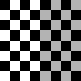
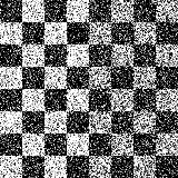
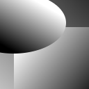
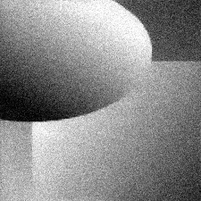
($a$) Checkerboard		($b$) Piecewise smooth

Figure 3: Synthetic test images (($a$) and ($b$), left) and their artificially generated noisy versions using Gaussian noise (($a$) and ($b$), right). The standard deviation of the Gaussian noise is 0.5 for ($a$) and 0.05 for ($b$).

The restored checkerboard images for classical TV and TGV are very similar owing to the piecewise constant nature of the ground truth. Moreover, a visible amount of punctual noise can still be observed inside the chess squares (consider the bright spots in the residual images). In contrast, for Condat-TV and the proposed TGV, where the results are also similar, these noise artifacts are attenuated (there are less bright spots inside the squares in the residual images). This experiment confirms that the proposed model preserves the property of Condat-TV to diminish punctual noise in the images containing textures, edges, and details (see Fig. 4).

($a$) TV denoising	($b$) Condat-TV denoising	($c$) TGV denoising	($d$) new-TGV denoising

Figure 4: Comparison of variational denoising results for the checkerboard test image (Figure 3($a$)). In the first and second row, the lower right part of the restored images and the absolute residual images are displayed, respectively. The parameters and quality metrics are as follows: ($a$) $\lambda^{*}=0.2$, PSNR=13.25, SSIM=0.3738, ($b$) $\lambda^{*}=0.19$, PSNR=13.31, SSIM=0.3856, ($c$) $\alpha_{1}^{*}=0.2$, PSNR=13.24, SSIM=0.3721, ($d$) $\alpha_{1}^{*}=0.19$, PSNR=13.31, SSIM=0.3850. Note that the proposed TGV method and the Condat-TV method are slightly more successful in removing the fairly high amount of noise. One can also observe that due to the piecewise constant nature of the test image, the results for TV-based and TGV-based methods are very similar.

For the piecewise smooth image, the results for the TV-based models and TGV-based model differ. TV and Condat-TV perform approximately alike and staircase artifacts appear in the restored images (see the bright stripes in the residual images), while for TGV and the proposed model, such artifacts do not appear (see Fig. 5). For both second-order models, the residual images are darker than TV and Condat-TV, indicating higher accuracy. This discussion shows that the proposed TGV model possesses the staircase artifact reduction capabilities of classical second-order TGV and the noise reduction capabilities of Condat-TV simultaneously.

($a$) TV denoising	($b$) Condat-TV denoising	($c$) TGV denoising	($d$) new-TGV denoising

Figure 5: Comparison of variational denoising results for the piecewise smooth test image (Figure 3($b$)). In the first and second row, the restored images and the absolute residual images are displayed, respectively. The chosen parameters are $\lambda^{*}=\alpha_{1}^{*}=0.07$, the quality metrics are as follows: ($a$) PSNR=37.20, SSIM=0.9426, ($b$) PSNR=37.54, SSIM=0.9480, ($c$) PSNR=40.74, SSIM=0.9886, ($d$) PSNR=41.01, SSIM=0.9886. Note the absence of staircasing artifacts for TGV-based models ($c$) and ($d$) in contrast to the TV-based models ($a$) and ($b$).

Moreover, we compare these variational denoising models for natural images (see the reference images in Figure 6), again with zero-mean additive Gaussian noise and standard deviation of $0.1$. These images contain partially smooth areas as well as textures, edges, and fine details. Based on the above discussion, we expect that the proposed model outperforms the competing methods in terms of accuracy and artifact reduction. Numerical results (Table LABEL:BLL) confirm that the proposed model can restore images with better accuracy (PSNR and SSIM values) whereas staircase artifacts are more attenuated (see Figures 7–10). That is, the new proposed TGV is more accurate in comparison to Condat’s TV and preserves the artifact-reducing property of the discrete classic second-order TGV (see again Figures 7–10). The resulting images are cleaner from noise and the PSNR and SSIM values are the highest in comparison to the other variational models. To observe more details of the reconstructed images, parts of the obtained images are also shown in a zoomed version in the figures.

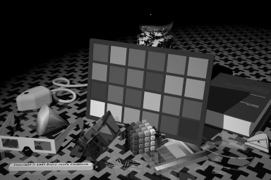
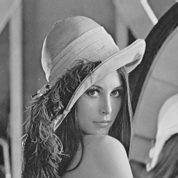
$(a)$ Fruits	$(b)$ Artificial	$(c)$ Lena
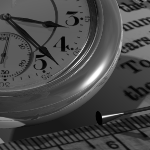
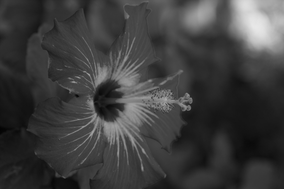
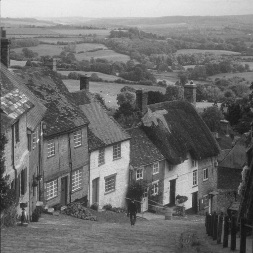
$(d)$ Watch	$(e)$ Flower	$(f)$ Goldhill

Figure 6: Reference images: gray scaled images in “png” format with the following sizes: $(a)$ Fruits ($512\times 512$ pixels), $(b)$ Artificial ($384\times 256$ pixels), $(c)$ Lena ($256\times 256$ pixels), $(d)$ Watch ($300\times 300$ pixels), $(e)$ Flower ($567\times 378$ pixels) and $(f)$ Goldhill ($512\times 512$ pixels).

$(a)$ reference image
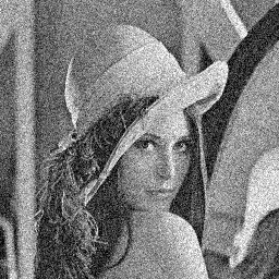
$(b)$ noisy image $(c)$ TV-restored	$(d)$ reference image: details
$(e)$ noisy image: details	$(f)$ TV-restored: details

Figure 7: Denoising experiment for the test image “Lena”: reference image, noisy image and restored image using the classic discrete TV model are shown in $(a)$, $(b)$ and $(c)$, respectively. Some details of the reference and noisy image are shown in $(d)$ and $(e)$. The details of the restored image using the classic discrete TV model is shown in $(f)$, where strong staircase artifacts around the interfaces are evident.

.

$(a)$ Condat-TV-restored
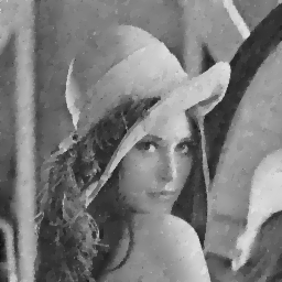
$(b)$ TGV-restored $(c)$ new-TGV-restored	$(d)$ Condat-TV-restored: details
$(e)$ TGV-restored: details	$(f)$ new-TGV-restored: details

Figure 8: Denoising experiment for the test image “Lena”: the restored images using Condat’s model, the second-order classic discrete TGV model and the proposed model are shown in $(a)$, $(b)$ and $(c)$, respectively. Some details are shown in $(d)$, $(e)$ and $(f)$. The obtained images by means of the TGV models are far better than the restored image using Condat’s TV model in terms of reducing staircase artifacts (for instance, look at the cheeks, in the restored images). In the result for classic discrete TGV, some unwanted narrow edges and speckles are visible in the smooth parts, whereas, in the proposed model, these kinds of effects have decreased significantly. On the other hand, the amount of noise in the image has been reduced using the proposed model. These distinguishing properties, beside the quantitative results (Table LABEL:BLL) show the benefits of the proposed method.

$(a)$ reference image
$(b)$ noisy image $(c)$ TV-restored	$(d)$ reference image: details
$(e)$ noisy image: details	$(f)$ TV-restored: details

Figure 9: Denoising experiment for the test image “Fruits”: reference image, noisy image and restored image using the classic discrete TV model are shown in $(a)$, $(b)$ and $(c)$, respectively. Some details of the reference and noisy image are shown in $(d)$ and $(e)$. The details of restored image using the classic discrete TV model is shown in $(f)$.

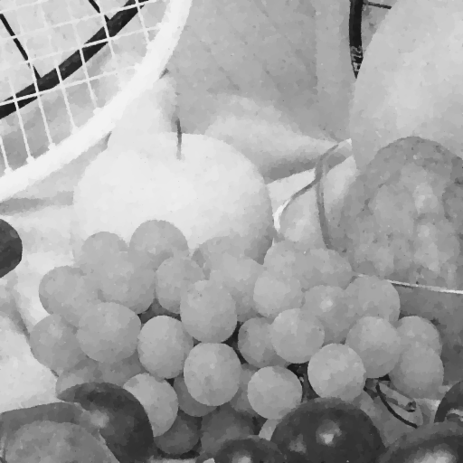
$(a)$ Condat-TV-restored
$(b)$ TGV-restored $(c)$ new-TGV-restored	$(d)$ Condat-TV-restored: details
$(e)$ TGV-restored: details	$(f)$ new-TGV-restored: details

Figure 10: Denoising experiment for the test image “Fruits”: the restored images using Condat’s TV model, the classic second-order discrete TGV model and the proposed model are shown in $(a)$, $(b)$ and $(c)$, respectively. Some details are shown in $(d)$, $(e)$ and $(f)$. The benefits of the proposed model are also evident in this experiment.

Table 1: Denoising problem results: the optimal regularization parameters $\lambda^{*}$ as well as the best PSNR and SSIM values for denoising of the test images are shown. Note that $\lambda^{*}$ is the best parameter $\lambda$ for the classic discrete TV model and Condat’s TV model for solving the denoising problems (66) $(a),(b)$ while for both TGV models, $\lambda^{*}=\alpha_{1}^{*}$ is the best parameter $\alpha_{1},$ where $\alpha_{0}=2\alpha_{1}$, $\alpha=(\alpha_{0},\alpha_{1})$ is chosen for the denoising problems (66) $(c),(d).$

Image	Fruits				Watch				Lena
Metric	$\lambda^{*}$	PSNR	SSIM		$\lambda^{*}$	PSNR	SSIM		$\lambda^{*}$	PSNR	SSIM
TV	0.080	30.15	0.8006		0.072	28.50	0.8048		0.074	27.85	0.7785
Condat	0.076	30.37	0.8080		0.066	28.80	0.8158		0.068	27.98	0.7832
TGV	0.080	30.21	0.8063		0.072	28.58	0.8101		0.074	27.97	0.7869
Proposed	0.076	30.42	0.8127		0.066	28.87	0.8203		0.068	28.08	0.7902
Image	Artificial				Flower				Goldhill
Metric	$\lambda^{*}$	PSNR	SSIM		$\lambda^{*}$	PSNR	SSIM		$\lambda^{*}$	PSNR	SSIM
TV	0.064	26.81	0.6273		0.088	33.36	0.8923		0.076	28.57	0.7284
Condat	0.058	27.04	0.6354		0.082	33.55	0.8963		0.070	28.71	0.7350
TGV	0.064	26.82	0.6275		0.088	33.75	0.9104		0.074	28.62	0.7304
Proposed	0.058	27.05	0.6355		0.082	33.90	0.9126		0.068	28.75	0.7367

We conclude the denoising experiments by showing the results for a color test image using the models and algorithms discussed in Subsection 3.6 with respect to the 3-channel RGB color space. For these experiments, the number of iterations is set to $N=1500$. In Figures 11 and 12, the reference image, the noisy image where zero-mean Gaussian noise with standard deviation $0.1$ has been added, as well as the results of four considered models are depicted. Also here, the proposed TGV model yields high-quality reconstructions in terms of accuracy and visual quality. The differences in the PSNR and SSIM values for the different models are, however, less pronounced.

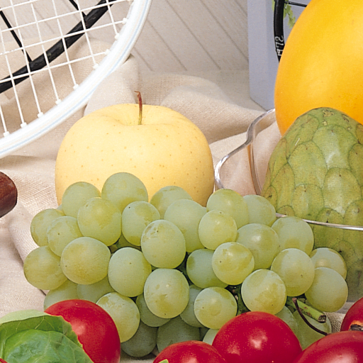
$(a)$ reference image
$(b)$ noisy image $(c)$ TV-restored	$(d)$ reference image: details
$(e)$ noisy image: details	$(f)$ TV-restored: details

Figure 11: Denoising experiment for the color test image “Fruits”: reference image, noisy image and restored image using the classic discrete TV model extended to color images are shown in $(a)$, $(b)$ and $(c)$, respectively, with details depicted in $(d)$, $(e)$ and $(f)$. The parameters and quality metrics for $(c)$ are as follows: $\lambda^{*}=0.12$, PSNR=30.05, SSIM=0.9524.

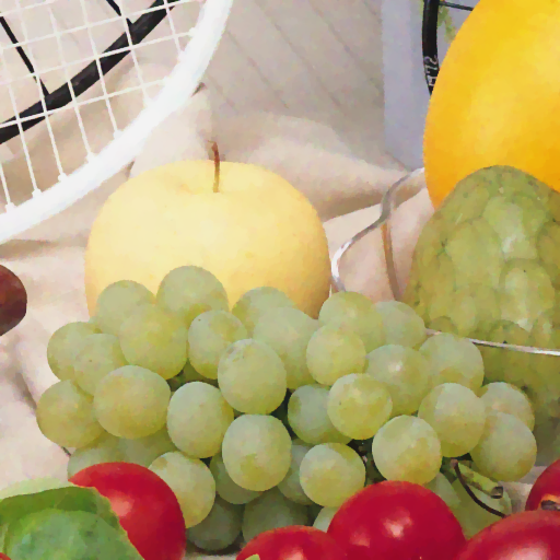
$(a)$ Condat-TV-restored
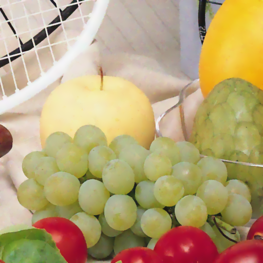
$(b)$ TGV-restored $(c)$ new-TGV-restored	$(d)$ Condat-TV-restored: details
$(e)$ TGV-restored: details	$(f)$ new-TGV-restored: details

Figure 12: Denoising experiment for the color test image “Fruits”: the restored images using Condat’s TV model, the classic second-order discrete TGV model and the proposed model extended to color images are shown in $(a)$, $(b)$ and $(c)$, respectively. Some details are depicted in $(d)$, $(e)$ and $(f)$. The parameters and quality metrics are as follows: ($a$) $\lambda^{*}=0.11$, PSNR=30.28, SSIM=0.9542, ($b$) $\lambda^{*}=0.11$, PSNR=30.12, SSIM=0.9511, ($c$) $\alpha_{1}^{*}=0.11$, PSNR=30.35, SSIM=0.9540.

5.2 Computation of TGV; classic TGV vs. proposed TGV

In this section the rotational invariance property of the classic discrete TGV and the proposed discrete TGV are compared. For three test images (see Figure 13), the classic discrete TGV values and the proposed discrete TGV values of the images as well as their $90^{\circ}$ rotated versions are calculated.

To compute an approximation of the classic discrete TGV and the proposed one, we solve the optimization problems (52) and (53), respectively, by means of the primal-dual algorithm (Algorithm 1). In order to solve (53), let $\tilde{L}^{*}=\left(\begin{array}[]{cccccc}L_{\bullet}^{*}&0&0&0&-\mathcal{E}^{new}\\ 0&L_{\bullet}^{*}&L_{\leftrightarrow}^{*}&L_{\updownarrow}^{*}&I\end{array}\right)$. Then, we can rewrite the constraint of (53) as

$$\tilde{L}^{*}(v_{\bullet},{w}_{\bullet},{w}_{\leftrightarrow},{w}_{\updownarrow},\omega)^{T}=(0,\mathcal{D}^{new}u)^{T}.$$

Now, set

$$z=(v_{\bullet},w_{\bullet},w_{\leftrightarrow},w_{\updownarrow},\omega)^{T},\ \ \mathcal{G}(z)=\alpha_{0}\|v_{\bullet}\|_{1}+\alpha_{1}\sum_{\star=\bullet,\leftrightarrow,\updownarrow}{\|{w}_{\star}\|_{1}},\ \ y=\left(\begin{array}[]{c}v\\ w\end{array}\right),\ \ \mathcal{F}(y)=I_{\{(0,\mathcal{D}^{new}u)\}}(y),\ \ A=\tilde{L}^{*}.$$

Then, problem (53) can be written in terms of (68). In order to employ Algorithm 1, note that the proximal operators for $\sigma\mathcal{F}^{*}$ and $\tau\mathcal{G}$ read as:

$$\text{prox}_{\sigma\mathcal{F}^{*}}(v,w)=(v,w-\sigma\mathcal{D}^{new}u),\quad\text{prox}_{\tau\mathcal{G}}(v_{\bullet},w_{\bullet},w_{\leftrightarrow},w_{\updownarrow},\omega)=(\bar{v}_{\bullet},\bar{w}_{\bullet},\bar{w}_{\updownarrow},\bar{w}_{\leftrightarrow},\bar{\omega}),$$

using the notation of (70). As a result, the primal-dual algorithm to solve (53) is outlined in Algorithm 3.

Data: Image $u\in\mathcal{U}_{\bullet}$, $\alpha=(\alpha_{0},\alpha_{1}),\alpha_{0}>0,\alpha_{1}>0$

Result: For the iteration number $N$, $z^{N}=(v_{\bullet}^{N},w_{\bullet}^{N},w_{\leftrightarrow}^{N},w_{\updownarrow}^{N},\omega^{N})$, is an approximation of the solution of the primal problem (53). Moreover, $y^{N}=(v^{N},w^{N})$ is an approximation of a solution of the dual problem (38) and the approximated new discrete TGV value is $\alpha_{0}\|v_{\bullet}\|_{1}+\alpha_{1}\sum_{\star=\bullet,\leftrightarrow,\updownarrow}{\|{w}_{\star}\|_{1}}$

Initialization:

Choose $\sigma>0$ and $\tau>0$ such that $\sigma\tau\|\tilde{L}\|^{2}<1$

Choose an arbitrary initial approximation of a primal solution $v_{\bullet}^{0}=\tilde{v}_{\bullet}^{0}\in\mathcal{U}_{\bullet}\times\mathcal{U}_{\bullet}\times\mathcal{U}_{\bullet}$, $w_{\star}^{0}=\tilde{w}_{\star}^{0}\in\mathcal{U}_{\star}\times\mathcal{U}_{\star}$, $\star=\bullet,\leftrightarrow,\updownarrow$, $\omega^{0}=\tilde{\omega}^{0}\in\mathcal{U}_{\leftrightarrow}\times\mathcal{U}_{\updownarrow}$

Choose an arbitrary initial approximation of a dual solution $v^{0}\in\bar{\mathcal{U}}_{\bullet}^{x}\times\bar{\mathcal{U}}_{\bullet}^{y}\times\mathcal{U}_{\times}$, $w^{0}\in\mathcal{U}_{\leftrightarrow}\times\mathcal{U}_{\updownarrow}$

while convergence criterion not met, for $k=0,1,\ldots$ do

      $v^{k+1}=v^{k}+\sigma(L^{*}_{\bullet}\tilde{v}_{\bullet}^{k}-\mathcal{E}^{new}\tilde{\omega}^{k})$

       $w^{k+1}=w^{k}+\sigma(L^{*}_{\bullet}\tilde{w}_{\bullet}^{k}+L^{*}_{\leftrightarrow}\tilde{w}_{\leftrightarrow}^{k}+L^{*}_{\updownarrow}\tilde{w}_{\updownarrow}^{k}-\mathcal{D}^{new}u+\tilde{\omega}^{k})$

       $v_{\bullet}^{k+1}=\text{shrink}_{\alpha_{0}\tau}(v_{\bullet}^{k}-\tau L_{\bullet}v^{k+1})$, $w_{\star}^{k+1}=\text{shrink}_{\alpha_{1}\tau}(w_{\star}^{k}-\tau L_{\star}w^{k+1})$, $\star=\bullet,\leftrightarrow,\updownarrow$

       $\omega^{k+1}=\omega^{k}-\tau(\text{div}^{new}v^{k+1}+w^{k+1})$

       $\tilde{v}_{\bullet}^{k+1}=2v_{\bullet}^{k+1}-v_{\bullet}^{k}$, $\tilde{w}_{\star}^{k+1}=2w^{k+1}_{\star}-w_{\star}^{k},\star=\bullet,\leftrightarrow,\updownarrow$, $\tilde{\omega}^{k+1}=2\omega^{k+1}-\omega^{k}$

end while

.

Algorithm 3 An algorithm for solving problem (53) and its dual form (38).

We employed Algorithm 3 with 1000 iterations in our simulations. Table 2 confirms that the proposed TGV has invariant values, up to numerical precision, for the original images and their 90 degree rotated versions.

$(a)$ Fruits	$(b)$ Barbara	$(c)$ Bike

Figure 13: The test images used for the 90^∘ isotropy testing problem. From left to right: Fruits, Barbara and Bike test image.

Image		Fruits		Barbara		Bike
Model/Rotation		TGV value	Error	TGV value	Error	TGV value	Error
TGV	$0^{\circ}$	587.0513	–	1326.9521	–	1720.4807	–
TGV	$90^{\circ}$	588.2140	1.1627	1329.7168	2.7647	1706.1456	14.3351
New TGV	$0^{\circ}$	632.2688	–	1421.8078	–	1806.2271	–
New TGV	$90^{\circ}$	632.2688	$4.55\times 10^{-13}$	1421.8078	$2.27\times 10^{-13}$	1806.2271	$1.14\times 10^{-12}$

Table 2: The values of the classic discrete TGV and the proposed discrete TGV for three test images and their $90^{\circ}$ rotated versions for the parameters $(\alpha_{0},\alpha_{1})=(0.14,0.07)$. Here, “error” is the absolute difference of the classic discrete TGV (proposed discrete TGV) value of the rotated image and the reference image.

6 Conclusion

In this paper, the idea of Condat’s discrete total variation is transferred to the second-order TGV. A new discrete second-order TGV model is designed based on the building blocks containing the definition of suitable grids, introducing new discrete derivative and divergence operators and proposing suitable linear conversion operators to guarantee some invariance properties. The proposed model is invariant with respect to $90^{\circ}$ rotations and preserves the benefits of Condat’s model in reducing noise for the areas containing textures, edges and details. Moreover, the new discrete TGV preserves the ability of the classic discrete TGV to diminish artifacts such as staircase artifacts, which are typical for discrete TV models. The same design principles can be applied for higher-order TGV or in higher dimensions to gain better results for imaging problems. While this can quite easily be done for specific cases, the development of a general framework requires some effort and can thus be regarded a subject of future work.

Appendix A A higher-order finite difference scheme for discrete TV

Recall that the basis for classic discrete TV [15, Section 3] is the following finite-difference approximation of the derivative:

$$f^{\prime}(x)\approx\frac{f(x+h)-f(x)}{h},$$ (73)

leading to the well-known two-point stencils of approximation order 1. In the following, instead of (73), we use the following central differences formula for TV denoising and compare it with the classic discrete TV:

$$f^{\prime}(x)\approx\frac{f(x+h)-f(x-h)}{2h}.$$ (74)

This approximation leads to a three-point finite difference stencil which has approximation order 2. Using symmetric boundary conditions for $u\in\mathbb{R}^{N_{1}\times N_{2}}$, we define the central differences discrete TV as follows:

$$\begin{array}[]{l}(\tilde{D}_{x}u)(n_{1},n_{2})=\frac{1}{2}(u(n_{1}+1,n_{2})-u(n_{1}-1,n_{2})),\\ (\tilde{D}_{y}u)(n_{1},n_{2})=\frac{1}{2}(u(n_{1},n_{2}+1)-u(n_{1},n_{2}-1)),\quad n_{1}=1,\ldots,N_{1},\ n_{2}=1,\ldots,N_{2},\\ \displaystyle\widetilde{TV}(u)=\sum_{n_{1}=1}^{N_{1}}\sum_{n_{2}=1}^{N_{2}}\sqrt{(\tilde{D}_{x}u)(n_{1},n_{2})^{2}+(\tilde{D}_{y}u)(n_{1},n_{2})^{2}}.\end{array}$$ (75)

The $\widetilde{\text{TV}}$ model can easily be tested using a primal-dual algorithm similar to Algorithm 4 below. Fig. 1, shows the reference image, a noisy version with zero-mean additive Gaussian noise of standard deviation $0.2$, and the restored images via classic discrete TV and central differences discrete TV according to (75). One clearly recognizes that the restored image using (75) is inaccurate and admits undesired checkerboard artifacts. The reason could be that locally, checkerboard-like images induce a vanishing discrete gradient when using a central-difference approximation and are hence preferred by the model. A similar effect can be observed when using a 5-point finite difference stencil and it appears that higher-order finite difference schemes are generally not suitable for variational denoising problems. When designing finite difference schemes for TV denoising, it seems to be essential to ensure that locally, the corresponding discrete gradient only vanishes where the image is constant. The property is certainly satisfied for the classical model that bases on (73).

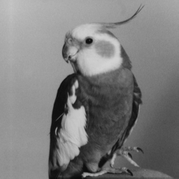
($a$) reference image	($b$) noisy image	($c$) TV-restored	($d$) $\widetilde{\text{TV}}$-restored

Figure 1: Test and comparison of the $\widetilde{\text{TV}}$ model. The chosen parameter is $\lambda^{*}=0.2$, the quality metrics are as follows: ($c$) PSNR=28.06, SSIM=0.8327, ($d$) PSNR=23.71, SSIM=0.3664. The change of derivative approximation scheme leads to clearly visible artifacts and a significant drop of reconstruction quality.

Appendix B Denoising algorithms and computational complexities

The primal-dual Algorithm 1 for the denoising problems (66) $(a)$–$(c)$ could be realized by the computational schemes outlined in Algorithms 4–6. We provide them for the sake of completeness and reproducibility. In particular, they allow for a rough estimate of the computational complexity of these algorithms for denoising a given $N_{1}\times N_{2}$ gray image in terms of flops per iteration. These estimates are summarized in Table 1. In summary, we obtain the following relations of the number of the flops of the proposed algorithm with TGV and Condat-TV:

$$\text{Number of flops for proposed TGV model}\approx 1.8\times\text{Number of flops for classic TGV model},$$

$$\text{Number of flops for proposed TGV model}\approx 1.8\times\text{Number of flops for Condat-TV model}.$$

The experimental MATLAB code in [25] confirms that these relations also approximately transfer to the utilized CPU time.

Data: Noisy image $f\in\mathbb{R}^{N_{1}\times N_{2}}$, $\lambda>0$

Result: For the iteration number $N$, $u^{N}$, is an approximation of the solution of the primal problem which is the obtained denoised image. Moreover, $w^{N}$ is an approximation of a solution of the dual problem

Initialization:

Choose $\sigma>0$ and $\tau>0$ such that $\sigma\tau\|\mathcal{D}\|^{2}<1$

Choose the initial approximation of a primal solution $u^{0}=\tilde{u}^{0}=f\in{\mathbb{R}}^{N_{1}\times N2}$

Choose an arbitrary initial approximation of a dual solution $w^{0}\in(\mathbb{R}^{N_{1}\times N_{2}})^{2}$

while convergence criterion not met, for $k=0,1,\ldots$ do

      $p^{k+1}=w^{k}+\sigma\mathcal{D}\tilde{u}^{k}$,  $\displaystyle w^{k+1}=\frac{\lambda p}{\max(|p|,\lambda)}$

       $\displaystyle u^{k+1}=\frac{u^{k}+\tau(\text{div}\,w^{k+1}+f)}{1+\tau}$

       $\tilde{u}^{k+1}=2u^{k+1}-u^{k}$

end while

Algorithm 4 An algorithm for solving the TV denoising problem (66) $(a)$.

Data: Noisy image $f\in\mathbb{R}^{N_{1}\times N_{2}}$, $\lambda>0$

Result: For the iteration number $N$, $z^{N}=(w_{\bullet}^{N},w_{\leftrightarrow}^{N},w_{\updownarrow}^{N},u^{N})$, is an approximation of the solution of the primal problem and $u^{N}$ is the obtained denoised image. Moreover, $w^{N}$ is an approximation of a solution of the dual problem

Initialization:

Choose $\sigma>0$ and $\tau>0$ such that $\sigma\tau\|L_{c}\|^{2}<1$, $L_{c}=\left(\begin{array}[]{cccc}L_{\bullet}^{*}&L_{\leftrightarrow}^{*}&L_{\updownarrow}&-\mathcal{D}\end{array}\right)$

Choose the initial approximation $u^{0}=\tilde{u}^{0}=f\in{\mathbb{R}}^{N_{1}\times N2}$

Choose an arbitrary initial approximation of a primal solution $w_{\star}^{0}=\tilde{w}_{\star}^{0}\in(\mathbb{R}^{N_{1}\times N_{2}})^{2}$, $\star=\bullet,\leftrightarrow,\updownarrow$

Choose an arbitrary initial approximation of a dual solution $w^{0}\in(\mathbb{R}^{N_{1}\times N_{2}})^{2}$

while convergence criterion not met, for $k=0,1,\ldots$ do

      $w^{k+1}=w^{k}+\sigma(L^{*}_{\bullet}\tilde{w}_{\bullet}^{k}+L^{*}_{\leftrightarrow}\tilde{w}_{\leftrightarrow}^{k}+L^{*}_{\updownarrow}\tilde{w}_{\updownarrow}^{k}-\mathcal{D}\tilde{u}^{k})$

       $w_{\star}^{k+1}=\text{shrink}_{\lambda\tau}(w_{\star}^{k}-\tau L_{\star}w^{k+1})$, $\star=\bullet,\leftrightarrow,\updownarrow$

       $\displaystyle u^{k+1}=\frac{u^{k}-\tau(\text{div}\,w^{k+1}-f)}{1+\tau}$

       $\tilde{w}_{\star}^{k+1}=2w^{k+1}_{\star}-w_{\star}^{k},\star=\bullet,\leftrightarrow,\updownarrow$

       $\tilde{u}^{k+1}=2u^{k+1}-u^{k}$

end while

Algorithm 5 An algorithm for solving the Condat-TV denoising problem (66) $(b)$.

Data: Noisy image $f\in\mathbb{R}^{N_{1}\times N_{2}}$, $\alpha=(\alpha_{0},\alpha_{1}),\alpha_{0}>0,\alpha_{1}>0$

Result: For the iteration number $N$, $z^{N}=(v^{N},w^{N},u^{N},\omega^{N})$, is an approximation of the solution of the primal problem and $u^{N}$ is the obtained denoised image. Moreover, $y^{N}=(\bar{v}^{N},\bar{w}^{N})$ is an approximation of a solution of the dual problem

Initialization:

Choose $\sigma>0$ and $\tau>0$ such that $\sigma\tau\|L_{\text{TGV}}\|^{2}<1,$ $L_{\text{TGV}}=\left(\begin{array}[]{cccc}I&0&0&-\mathcal{E}\\ 0&I&-\mathcal{D}&I\end{array}\right)$

Choose the initial approximation $u^{0}=\tilde{u}^{0}=f\in\mathbb{R}^{N_{1}\times N_{2}}$

Choose an arbitrary initial approximation of a primal solution $v^{0}=\tilde{v}^{0}\in(\mathbb{R}^{N_{1}\times N_{2}})^{3}$,

$w^{0}=\tilde{w}^{0}\in(\mathbb{R}^{N_{1}\times N_{2}})^{2},\omega^{0}=\tilde{\omega}^{0}\in(\mathbb{R}^{N_{1}\times N_{2}})^{2}$

Choose an arbitrary initial approximation of a dual solution $\bar{v}^{0}\in(\mathbb{R}^{N_{1}\times N_{2}})^{3}$, $\bar{w}^{0}\in(\mathbb{R}^{N_{1}\times N_{2}})^{2}$

while convergence criterion not met, for $k=0,1,\ldots$ do

      $\bar{v}^{k+1}=\bar{v}^{k}+\sigma(\tilde{v}^{k}-\mathcal{E}\tilde{\omega}^{k})$

       $\bar{w}^{k+1}=\bar{w}^{k}+\sigma(\tilde{w}^{k}-\mathcal{D}\tilde{u}^{k}+\tilde{\omega}^{k})$

       $v^{k+1}=\text{shrink}_{\alpha_{0}\tau}(v^{k}-\tau\bar{v}^{k+1})$, $w^{k+1}=\text{shrink}_{\alpha_{1}\tau}(w^{k}-\tau\bar{w}^{k+1})$

       $\displaystyle u^{k+1}=\frac{u^{k}-\tau(\text{div}\bar{w}^{k+1}-f)}{1+\tau}$, $\omega^{k+1}=\omega^{k}-\tau(\text{div}\bar{v}^{k+1}+\bar{w}^{k+1})$

       $\tilde{v}^{k+1}=2v^{k+1}-v^{k}$, $\tilde{w}^{k+1}=2w^{k+1}-w^{k},$

       $\tilde{u}^{k+1}=2u^{k+1}-u^{k}$, $\tilde{\omega}^{k+1}=2\omega^{k+1}-\omega^{k}$

end while

Algorithm 6 An algorithm for solving the second-order TGV denoising problem (66) $(c)$.

Operators/Model	TV	Condat-TV	TGV	Proposed
Number of square roots	$N_{1}N_{2}$	$3N_{1}N_{2}$	$2N_{1}N_{2}$	$4N_{1}N_{2}$
Number of comparisons	$N_{1}N_{2}$	$3N_{1}N_{2}$	$2N_{1}N_{2}$	$4N_{1}N_{2}$
		Number of flops
Gradients and divergences	$4N_{1}N_{2}$	$4N_{1}N_{2}$	$16N_{1}N_{2}$	$16N_{1}N_{2}$
Grid converters and adjoints	–	$24N_{1}N_{2}$	–	$30N_{1}N_{2}$
Shrinkage operator	$7N_{1}N_{2}$	$21N_{1}N_{2}$	$17N_{1}N_{2}$	$31N_{1}N_{2}$
Main body	$11N_{1}N_{2}$	$41N_{1}N_{2}$	$54N_{1}N_{2}$	$82N_{1}N_{2}$
Total number of flops	$22N_{1}N_{2}$	$90N_{1}N_{2}$	$87N_{1}N_{2}$	$159N_{1}N_{2}$

Table 1: Computational complexity per iteration of the denoising algorithms for a given $N_{1}\times N_{2}$ noisy image, i.e., TV (Algorithm 4), Condat-TV (Algorithm 5), classical second-order TGV (Algorithm 6), and the proposed TGV (Algorithm 2).

References

- [1] Abergel, R., Moisan, L.: The Shannon total variation. J. Math Imaging Vis., 59, 341–370 (2017).
- [2] Alter, F., Caselles, V., Chambolle, A.: Evolution of characteristic functions of convex sets in the plane by the minimizing total variation flow. Interfaces Free Bound., 7, 29–53 (2005).
- [3] Bauschke, H.H., Combettes, P.L.: Convex Analysis and Monotone Operator Theory in Hilbert Spaces, 2nd ed. Springer, New York (2017).
- [4] Bredies, K.: Recovering piecewise smooth multichannel images by minimization of convex functionals with total generalized variation penalty. Lecture Notes in Computer Science, 8293, 44–77 (2014).
- [5] Bredies, K. and Holler, M.: A TGV-based framework for variational image decompression, zooming and reconstruction. Part I: Analytics. SIAM J. Imaging Sci., 8(4), 2814–2850 (2015).
- [6] Bredies, K. and Holler, M.: A TGV-based framework for variational image decompression, zooming and reconstruction. Part II: Numerics. SIAM J. Imaging Sci., 8(4), 2851–2886 (2015).
- [7] Bredies, K. and Holler, M.: Higher-order total variation approaches and generalisations. Inverse Problems, 36(12), 123001 (2020).
- [8] Bredies, K. and Holler, M.: Regularization of linear inverse problems with total generalized variation, Journal of Inverse and Ill-posed Problems, 22(6), 871–913 (2014).
- [9] Bredies, K., Holler, M., Storath, M. and Weinmann, A.: Total Generalized Variation for Manifold-valued Data, SIAM J. Imaging Sci., 11(3), 1785–1848 (2018).
- [10] Bredies, K., Kunisch, K. and Pock, T.: Total generalized variation, SIAM J. Imaging Sci., 3, 492–526 (2010).
- [11] Bredies, K., Nuster, R. and Watschinger, R.: TGV-regularized inversion of the Radon transform for photoacoustic tomography. Biomedical Optics Express, 11(2), 994–1019 (2020).
- [12] Buades, A., Coll, B. and Morel, J.M.: Image denoising methods. A new nonlocal principle. SIAM Rev., 52, 113–147 (2010).
- [13] Chambolle, A.: An Algorithm for Total Variation Minimization and Applications, J. Math Imaging Vis., 20, 89–97 (2004).
- [14] Chambolle, A.: Finite-differences discretizations of the Mumford-Shah functional, Mathematical Modelling and Numerical Analysis, 33, 261–288 (1999).
- [15] Chambolle, A., Caselles, V., Cremers, D., Novaga, M. and Pock, T.: An Introduction to Total Variation for Image Analysis, in Theoretical Foundations and Numerical Methods for Sparse Recovery, Germany, Berlin: De Gruyter, vol. 9, 263–340 (2010).
- [16] Chambolle, A. and Pock, T.: A first-order primal-dual algorithm for convex problems with applications to imaging, J. Math Imaging Vis., 40, 120–145 (2011).
- [17] Chambolle, A. and Pock, T.: Crouzeix–Raviart approximation of the total variation on simplicial meshes, J. Math Imaging Vis., 62, 872–899 (2020).
- [18] Chambolle, A., Levine, S.E., Lucier, B. J.: An upwind finite-difference method for total variation based image smoothing. SIAM J. Imaging Sci., 4, 277–299 (2011).
- [19] Condat, L.: Discrete total variation: new definition and minimization, SIAM Journal on Imaging Sciences, 10(3), 1258–1290 (2017).
- [20] Dabov, K., Foi, A., Katkovnik, V. and Egiazarian, K.: Image denoising by sparse 3-D transform-domain collaborative filtering. IEEE Trans. Image Process., 16, 2080–2095 (2007).
- [21] Ghazel, M., Freeman, G.H. and Vrscay, E.R.: Fractal image denoising. IEEE Transactions on Image Processing. 12, 1560–1578 (2003).
- [22] Hohm, K., Storath, M. and Weinmann, A.: An algorithmic framework for Mumford-Shah regularization of inverse problems in imaging, Inverse Problems, 31, 115011 (2015).
- [23] Hosseini, A.: New discretization of total variation functional for image processing tasks, Signal Processing: Image Communication, 78, 62–76 (2019).
- [24] Hosseini, A. and Bazm, S.: The second-order Shannon total generalized variation for image restoration, Signal Processing, 204, 108848 (2023).
- [25] Hosseini, A. and Bredies, K.: A Second-Order TGV Discretization with Some Invariance Properties (Supplementary MATLAB files), Mendeley Data, doi:10.17632/wbwfxht3hb (2023).
- [26] Hu, Y., Wang, N., Tao, D., Gao, X. and Li, X.: Serf: a simple, effective, robust, and fast image super-resolver from cascaded linear regression, IEEE Trans. Image Process., 25, 4091–4102 (2016).
- [27] Huber, R., Haberfehlner, G., Holler, M., Kothleitner, G. and Bredies, K.: Total Generalized Variation regularization for multi-modal electron tomography. Nanoscale, 11, 5617–5632 (2019).
- [28] Knoll, F., Holler, M., Koesters, T., Otazo, R., Bredies, C. and Sodickson, D.: Joint MR-PET reconstruction using a multi-channel image regularizer, IEEE Trans. Med. Image., 36(1), 1–16 (2017).
- [29] Knoll, F., Bredies, K., Pock, T. and Stollberger, R.: Second order total generalized variation (TGV) for MRI, Magnetic Resonance in Medicine, 65(2), 480–491 (2011).
- [30] Langkammer, C., Bredies, K., Poser, B.A, Barth, M., Reishofer, G., Fan, A.P., Bilgic, B., Fazekas, F., Mainero, C. and Ropele, S.: Fast Quantitative Susceptibility Mapping using 3D EPI and Total Generalized Variation, NeuroImage, 111, 622–630 (2015).
- [31] Lore, K.G., Akintayo, A. and Sarkar, S.: LLNEt: A deep autoencoder approach to natural low-light image enhancement, Pattern Recognit., 61, 650–662 (2015).
- [32] Papafitsoros, K. and Bredies, K.: A study of the one dimensional total generalised variation regularisation problem. Inverse Problems and Imaging, 9(2), 511–550 (2015).
- [33] Perona, P. and Malik, J.: Scale-space and edge detection using anisotropic diffusion, IEEE Trans. Pattern Anal. Mach. Intell., 12, 629–639 (1990).
- [34] Rudin, L. I., Osher, S., Fatemi, E.: Nonlinear total variation based noise removal algorithms, Phys. D, 60, 259–268 (1992).
- [35] Sardy, S., Tseng, P. and Bruce, A.: Robust wavelet denoising. IEEE Trans. Sig. Process., 49, 1146–1152 (2001).
- [36] Storath, M., Brandt, C., Hofmann, M., Knopp, T., Salamon, J., Weber, A. and Weinmann, A.: Edge preserving and noise reducing reconstruction for magnetic particle imaging, IEEE Tran. Med. Imag., 36, 74–85 (2016).
- [37] Storath, M. and Weinmann, A.: Fast partitioning of vector-valued images, SIAM J. Imaging Sci., 7(3), 1826–1852 (2014).
- [38] Valkonen, T., Bredies, K. and Knoll, F.: Total Generalized Variation in Diffusion Tensor Imaging, SIAM J. Imaging Sci., 6(1), 487–525 (2013).
- [39] Weickert, J.: Anisotropic diffusion in Image Processing, Teubner, Stuttgart (1998).
- [40] Wang, Z., Bovik, A.C., Sheikh, H.R., Simoncelli, E.P.: Image quality assessment: from error visibility to structural similarity, IEEE Trans. Image Process., 13(4), 600–612 (2004).
- [41] Wang, N., Tao, D., Gao, X., Li, X. and Li, J.: A comprehensive survey to face hallucination, Int. J. Comput. Vis., 106, 9–30 (2014).
- [42] Wen, Y.W., Michael, K.N. and Ching, W.K.: Iterative algorithms based on decoupling of deblurring and denoising for image restoration. SIAM J. Sci. Comput., 30, 2655–2674 (2008).