RIS-Aided MIMO Systems with Hardware Impairments: Robust Beamforming Design and Analysis

Abstract

Reconfigurable intelligent surface (RIS) has been anticipated to be a novel cost-effective technology to improve the performance of future wireless systems. In this paper, we investigate a practical RIS-aided multiple-input-multiple-output (MIMO) system in the presence of transceiver hardware impairments, RIS phase noise and imperfect channel state information (CSI). Joint design of the MIMO transceiver and RIS reflection matrix to minimize the total average mean-square-error (MSE) of all data streams is particularly considered. This joint design problem is non-convex and challenging to solve due to the newly considered practical imperfections. To tackle the issue, we first analyze the total average MSE by incorporating the impacts of the above system imperfections. Then, in order to handle the tightly coupled optimization variables and non-convex NP-hard constraints, an efficient iterative algorithm based on alternating optimization (AO) framework is proposed with guaranteed convergence, where each subproblem admits a closed-form optimal solution by leveraging the majorization-minimization (MM) technique. Moreover, via exploiting the special structure of the unit-modulus constraints, we propose a modified Riemannian gradient ascent (RGA) algorithm for the discrete RIS phase shift optimization. Furthermore, the optimality of the proposed algorithm is validated under line-of-sight (LoS) channel conditions, and the irreducible MSE floor effect induced by imperfections of both hardware and CSI is also revealed in the high signal-to-noise ratio (SNR) regime. Numerical results show the superior MSE performance of our proposed algorithm over the adopted benchmark schemes, and demonstrate that increasing the number of RIS elements is not always beneficial under the above system imperfections.

I Introduction

Recently, reconfigurable intelligent surface (RIS) has attracted much attention in wireless communications due to its ability of reshaping the wireless propagation environment dynamically. Specifically, the RIS is composed of a large number of passive and low-cost reflecting elements, which can adjust the phase of the incident signal towards the target direction with the aid of a smart controller and thus create the favorable communication channels. Since the RIS does not require costly radio frequency (RF) chains, it can be regarded as a cost-effective solution for improving the spectrum and energy efficiency of future wireless networks. Inspired by the high flexibility of the RIS deployment, its integration with the cutting-edge techniques, such as unmanned aerial vehicle (UAV) communications[1], mmWave communications[2], secure communications[3], wireless power transfer[4] and so on, has also triggered an upsurge research interest [5].

Considering the above significant benefits of the RIS, there have been plenty of works focusing on the RIS-aided communication systems[6, 7, 8, 9, 10, 11, 12, 13, 14, 15, 16, 17]. These works can be classified by different design objectives, e.g., the transmit power minimization[6, 7], the rate maximization[8, 9, 10], the mean-square-error (MSE) minimization[11, 12, 13], the energy efficiency maximization[14, 15], the minimum signal-to-interference-plus-noise-ratio (SINR) maximization[16]. In addition to the above considered narrowband scenarios, the sum-rate maximization of the RIS-aided orthonormal frequency division multiplexing (OFDM) system over the frequency-selective channels has also been studied [18, 19, 20]. However, all the above works rely on the use of ideal hardware.

Nevertheless, the transmitter and receiver usually suffer from non-negligible hardware impairments (HWIs) in practice, such as amplifier nonlinearities, analog-to-digital converters (ADCs) nonlinearities, digital-to-analog converters (DACs) nonlinearities, in-phase (I) and quadrature (Q) imbalance and oscillator phase noise, etc [21, 22]. Even taking the compensation algorithms, the residual hardware impairments [23] still cause the mismatch between the intended signal and the actual radiated signal, thereby leading to the degradation of system performance, such as the ergodic capacity, achievable rate, MSE [24, 25, 26]. Specifically, the authors of [24] analyzed the detrimental effects of transceiver hardware impairments on the ergodic capacity, the outage probability, and the spectral efficiency of the RIS-aided single-input-single-output (SISO) system. Moreover, the authors in [25] analyzed the effects of transceiver hardware impairments on the ergodic capacity, showing that transceiver hardware impairments imposes a finite limit on the ergodic capacity, which is unrelated to the number of RIS elements and BS antennas. To alleviate this issue, there have sprung up some works aiming at RIS-aided communication systems with transceiver hardware impairments [27, 28, 29]. For example, to ensure the maximum secrecy rate, the authors in [27] studied the robust transmission design for a RIS-aided secure communication system in the presence of transceiver hardware impairments. In [28], the robust transmit precoder and RIS reflection matrix were jointly optimized to maximize the received signal-to-noise-ratio (SNR) of the RIS-aided multi-input-single-output (MISO) system via the generalized Rayleigh quotient and majorization-minimization (MM) algorithm.

In addition, taking into account practical finite-resolution phase shifts, the hardware impairments at the RIS are usually modeled as RIS phase noise. Currently, there are two popular distributions used for modeling the RIS phase noise, e.g., the uniform and the Von Mises distributions[30]. Accordingly, the joint impacts of RIS phase noise and transceiver hardware impairments on the RIS-assisted communications were investigated in [31, 32, 33, 25, 34, 35]. For example, the authors in [31] modeled the random RIS phase noise following a zero-mean Von Mises distribution and studied the MSE minimization problem by jointly optimizing the transceiver and RIS reflection matrix, where the closed-form continuous phase shifts are derived using MM technique. Also, the inevitable phase errors at the RIS affected the diversity order [25], hence it degraded the signal-to-noise-plus-distortion ratio which leads to a significant reduction in the ergodic capacity. On the other hand, the work in [34] considered the uniformly distributed RIS phase noise and unveiled the impact of phase shift errors and transmission hardware impairments on the system sum throughput for the RIS-aided wireless-powered Internet of Things (IoT) network, in which wireless energy transfer and information receptions are studied. With the same uniformly distributed RIS phase noise, the authors in [35] aimed to maximize the achievable rate by designing the phase shifts using the condition of statistical channel state information (CSI), where the iterative genetic algorithm (GA) is applied.

It is clear that the aforementioned works are all conducted under the assumption of perfect CSI. In general, perfect CSI is hard to obtain due to channel estimation errors, channel feedback delays and quantization errors. It is therefore meaningful to investigate the joint optimization of the MIMO transceiver and RIS reflection matrix by incorporating the effects of both system hardware impairments and imperfect CSI. To our best knowledge, there were only limited studies considering the RIS-aided wireless networks with both non-negligible hardware impairments and imperfect CSI[36, 37, 38]. Specifically, the authors in [36] studied the robust beamforming design for the transmit power minimization where the joint impacts of transceiver hardware impairments and statistical CSI errors is considered. However, the impact of RIS phase noise is neglected in this work. Meanwhile, the works[37, 38] investigated the channel estimation methods accounting for both transceiver hardware impairments and RIS phase noise. Armed with the estimated channels, these two works further studied the joint beamforming design for the channel capacity and the achievable sum spectral efficiency, respectively. Note that only the single-antenna nodes or users are considered in all these above works. To the best of our knowledge, there has been no literature investigating the comprehensive impacts of the transceiver hardware impairments, RIS phase noise and imperfect CSI on the RIS-aided MIMO system, which thus motivates this work.

In this paper, we consider an RIS-aided point-to-point MIMO system in the presence of transceiver hardware impairments, RIS phase distortion and imperfect CSI. It is known that different performance metrics of RIS-aided MIMO communications such as the sum rate, the total transmit power and the energy efficiency have been well optimized. These performance metrics essentially represent different trade-offs among the MSEs of multiple data streams[39]. As such, we aim to minimize the total MSE of the considered system by jointly designing the MIMO transceiver and the RIS reflection matrix subject to the transmit power constraint and the discrete unit-modulus constraints at the RIS. Unfortunately, since the integration of the above three types of system imperfections renders the optimization problem much complicated, most existing numerical algorithms adopted by the RIS-relevant works cannot be straightforwardly applied. The main contributions of our work are summarized as follows.

• This is the first paper to investigate the joint impacts of transceiver hardware impairments, RIS phase noise and imperfect CSI on the RIS-aided point-to-point MIMO systems. We formulate the joint transceiver and RIS reflection matrix design problem as the total average MSE minimization problem, where the analytical expression is derived in the presence of statistical CSI errors and RIS phase noise. Different from the existing research focusing on the single-antenna users, our work considers the general MIMO system setup, thereby leading to an intractable matrix-valued optimization problem. Note that the existing optimization methods are inapplicable to our problem.

• We propose an MM-based algorithm framework to solve the intractable matrix-valued optimization problem with guaranteed convergence. Specifically, for the transmit precoder design with the intractable objective function, a locally tight lower bound is found using the MM technique. Then, based on Karush-Kuhn-Tucker (KKT) conditions, the optimal transmit precoder is derived in closed-form in each iteration. Similarly, we also apply the MM technique to solve the non-convex discrete phase constraints at the RIS, namely the two-tier MM-based algorithm. In addition, by exploiting the unit-modulus discrete phase constraints, we propose a novel modified Riemannian gradient ascent (RGA) algorithm to obtain the sub-optimal solution of the RIS reflection matrix.

• We reveal that an irreducible MSE floor exists in the high-SNR regime. Specifically, we derive an explicit expression of the MSE floor and analyze the impacts of the transceiver hardware impairments, the RIS phase noise, and the imperfect CSI on the average MSE in the special case of RIS-aided MISO system, individually. The simulation results demonstrate the impacts of different system imperfections on the system’s performance, providing some practical insights for implementing the RIS-aided MIMO system.

The remainder of this paper is organized as follows. Section II introduces the system model and problem formulation. The joint robust MIMO transceiver and RIS reflection matrix design is presented in Section III. Section IV discusses the optimality of the proposed MM-based AO algorithm and analyzes the MSE performance under some special cases. Numerical results are shown in Section V. Finally, Section VI concludes this paper.

Notations: The notation $\mathbb{E}$ represents the expectation on the random variables. ${\mathbb{C}^{M\!\times\!N}}$ denotes the $M\times N$ complex space. $\bf{A}^{\star}$, ${\bf{A}}^{T}$, ${\bf{A}}^{H}$, ${\bf{A}}^{-1}$ and $\rm Tr({\bf{A}})$ represent the conjugate, transpose, Hermitian, inverse and trace of matrix ${\bf{A}}$, respectively. ${\bf{I}}_{d}$ denotes a $d\times d$ identity matrix, and $[{\bf{a}}]_{i}$ denotes the $i$-th element of vector ${\bf{a}}$. $[{\bf{A}}]_{ij}$ represents the $(i,j)$-th element of matrix ${\bf{A}}$. The notations ${\rm vec}\left({\bf{A}}\right)$, $\otimes$ and $\odot$ denote the matrix vectorization, Kronecker product and Hadamard product, respectively. ${\rm{diag}}({\bf{a}})$ indicates a square diagonal matrix whose diagonal elements consist of a vector ${\bf{a}}$. ${\rm{\widetilde{diag}}}({\bf{A}})$ represents a square diagonal matrix whose diagonal elements are the same as those of the matrix ${\bf{A}}$. $\Re\{\}$ returns the real part of the complex input, and $|a|$ represents the modulus of the complex input $a$. The words “with respect to” and “ circularly symmetric complex Gaussian” are abbreviated as “w.r.t.” and “CSCG”, respectively. ${\cal{U}}[a,b]$ denotes the uniform distribution over the interval $[a,b]$. The main symbols used in this paper are listed in Table I.

TABLE I: List of Symbols

Symbol	Description	Symbol	Description
$N_{T}/N_{R}$	Number of BS/user antennas	$M/d$	Number of RIS elements/data streams
${\bf{x}}$	Transmit data symbols	${\bf{s}}/{\bf{y}}$	Transmitted/Received signal at BS/user
${\bf{W}}/{\bf{C}}$	Transmit precoder/Linear equalizer	$b$	Number of quantization bits
${{\bm{\kappa}}_{T}}/{{\bm{\kappa}}_{R}}$	Transmitter/Receiver distortion noise	${\beta_{T}}/{\beta_{R}}$	Normalized transmitter’s/receiver’s distortion level
${{\bf{H}}_{\rm cas}}$	Cascaded BS-RIS-user channel	${{\bf{G}}_{m}}$	Compound channel associated
			with $m$-th RIS element
${{\bf{H}}_{d}}/{{\bf{H}}_{I}}/{{\bf{H}}_{r}}$	BS-user/BS-RIS/RIS-user channel	${{\bf{\bar{H}}}_{d}}/{{\bf{\bar{G}}}_{m}}$	Estimated direct/compound channel
$\Delta{\bf{H}}_{d}/\Delta{\bf{G}}_{m}$	CSI errors	${\sigma_{d}^{2}}/{\sigma_{m}^{2}}$	Channel estimation inaccuracy
${\bm{\Theta}}/{\bm{\theta}}$	RIS reflection matrix/vector	${\phi_{m}}/{\Delta\phi_{m}}$	RIS phase shift/distortion
$P$	Transmit power	$\sigma^{2}$	Noise variance
$\epsilon_{b}$	Average phase distortion level	${\bf{\bar{H}}}_{\bm{\theta}}$	Available cascaded BS-RIS-user channel
${\bf{T}}^{\rm SI}_{{\bf{W}}}$	Joint impacts of system imperfections	${\bf{\ H}}_{\rm cat}$	Concatenated channel
${\bf{T}}^{\rm cas}_{{\bf{W}},\bm{\theta}}$/${\bf{T}}^{\rm com}_{{\bf{W}}}$	Received signal covariance matrix	$\nu_{I}$/$\nu_{r}$	Complex channel gain of the LoS path
	associated with ${\bf{\bar{H}}}_{\bm{\theta}}$/${\bf{\bar{G}}}_{m}$		for the BS-RIS/RIS-user channel
${\bf a}_{TX}$/${\bf a}_{RX}$	Array response vector at BS/user	${\bf a}_{RA}$/${\bf a}_{RD}$	Array response vector of AoA/AoD at RIS

II System Model and Problem Formulation

II-A System Model

As shown in Fig. 1, a narrowband RIS-aided MIMO communication system is considered, where an RIS equipped with $M$ reflecting elements is deployed to assist in downlink communications from a base station (BS) equipped with $N_{T}$ antennas to a user equipped with $N_{R}$ antennas. Denoted by ${\bf{x}}\in{\mathbb{C}^{d\times 1}}$ with $d\leq{\rm{min}}(N_{T},N_{R})$ and $\mathbb{E}\left[{{\bf{x}}{{\bf{x}}^{H}}}\right]\!=\!{{\bf{I}}_{d}}$ the transmit data symbols, the transmit signal at the BS considering the realistic hardware impairments is then expressed as

$${\bf{s}}={{\bf{W}}}{{\bf{x}}}+{{\bm{\kappa}}_{T}},\vspace{-2mm}$$ (1)

where ${\bf{W}}\in{\mathbb{C}^{N_{T}\times d}}$ represents the transmit precoder and ${{\bm{\kappa}}_{T}}\in\mathbb{C}^{N_{T}\times 1}$ denotes the transmitter distortion noise, which models the aggregate residual hardware impairments after calibration or pre-distortion[21] at the BS and is independent of the data symbols x. The elements of ${{\bm{\kappa}}_{T}}$ are usually assumed to be CSCG distributed variables with zero mean and variance being proportional to the transmit power of each antenna[40], namely, ${{\bm{\kappa}}_{T}}\!\sim\!{\cal C}{\cal N}({{\bf{0}},{\beta_{T}^{2}}{\rm{\widetilde{diag}}}({{{{\bf{W}}}{{\bf{W}}}^{H}}})})$, where ${\beta_{T}}\in[0,1]$ characterizes the normalized distortion level whose value is much less than 1[41]. The BS-user channel, the BS-RIS channel and the RIS-user channel are denoted as ${\bf{H}}_{d}\in\mathbb{C}^{N_{R}\times N_{T}}$, ${\bf{H}}_{I}\in\mathbb{C}^{N_{T}\times M}$ and ${\bf{H}}_{r}\in\mathbb{C}^{N_{R}\times M}$, respectively. The reflection coefficient of the $m$-th RIS reflecting element is given by ${{\theta}}_{m}=a_{m}e^{j\phi_{m}},m\in\!\mathcal{M}\!=\!\{1,2,\cdots,M\}$, where $a_{m}$ and $\phi_{m}$ denote the reflection amplitude and phase shift, respectively, and the maximum reflection amplitude $a_{m}=1$ is assumed for simplicity. As such, the cascaded BS-RIS-user channel can be expressed as ${\bf{H}}_{\rm cas}={\bf{H}}_{d}+{\bf{H}}_{r}{\bm{\Theta}}{\bf{H}}_{I}^{H}$, where $\bm{\Theta}\!=\!\rm diag\left([\theta_{1},\cdots,\theta_{M}]\right)$ stands for the RIS reflection matrix. Specifically, the direct link between the BS and the user may be unavailable due to short wavelengths at high frequencies and severe blockage from buildings and trees[42] in the realistic scenarios. As a remedy, the RIS can be deployed in the high altitudes to intelligently reflect the incident signal to the target user for assisting in wireless communications. In such scenarios, the RIS-related channels are assumed to have only LoS components.

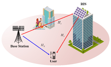
Figure 1: An RIS-aided point-to-point MIMO communication system.

Due to the passive reflection property of the RIS, the cascaded BS-RIS-user channel estimation is generally more cost-effective than the separate channel estimation, in which the BS-RIS channel ${\bf{H}}_{I}$ and the RIS-user channel ${\bf{H}}_{r}$ are estimated independently. In terms of our work, we assume that channel reciprocity holds, based on which the cascaded BS-RIS-user channel estimation is performed at the BS via the uplink pilot transmission. Specifically, we first divide the whole uplink training phase into $M+1$ subphases. The “ON/OFF” mode is adopted by each RIS reflecting element by setting $a_{m}\!=\!1/0,~{}\forall m\!\in\!\mathcal{M}$. In the first subphase, the direct channel ${\bf{H}}_{d}$ is estimated by setting all the reflecting elements to “OFF”. Then, the compound channel ${\bf{G}}_{m}={\bf{h}}_{r,m}{\bf{h}}_{I,m}^{H}$ associated with the $m$-th RIS reflecting element is obtained by turning the $m$-th RIS reflecting element “ON” while keeping the others “OFF”, where ${\bf{h}}_{r,m}$ and ${\bf{h}}_{I,m}$ denote the $m$-th columns of ${\bf{H}}_{r}$ and ${\bf{H}}_{I}$, respectively. In this context, the cascaded BS-RIS-user channel ${\bf{H}}_{\rm cas}$ is reexpressed as

$${\bf{H}}_{\rm cas}={\bf{H}}_{d}+{\sum\nolimits_{i=1}^{M}{\theta_{m}}{\bf{G}}_{m}}.$$ (2)

Then, the received signal $\rm\bf{y}$ at the user can be written as

$${{\bf{y}}}=\underbrace{{\bf{H}}_{\rm cas}\left({{\bf{W}}}{{\bf{x}}}+{{\bm{\kappa}}_{T}}\right)+{\rm{\bf{n}}}}_{\rm{\bf{\tilde{y}}}}+{{\bm{\kappa}}_{R}},$$ (3)

where $\tilde{\bf{y}}\in{\mathbb{C}^{N_{R}\times 1}}$ denotes the undistorted received signal and ${\bf{n}}\in{\mathbb{C}^{N_{R}\times 1}}$ represents the additive white Gaussian noise (AWGN) drawn from $\mathcal{C}\mathcal{N}\left({\bf{0}},\sigma^{2}{\bf{I}}\right)$. Analogous to the definition of ${{\bm{\kappa}}_{T}}$, ${{\bm{\kappa}}_{R}}\sim{\cal C}{\cal N}({\bf{0}},{\beta_{R}^{2}}{\rm{\widetilde{diag}}}\left({\mathbb{E}\left[{{\bf{\tilde{y}}}{\bf{\tilde{y}}}^{H}}\right]}\right))$ denotes the CSCG distributed receiver distortion noise, where ${\beta_{R}}$ indicates the distortion level at the user and

$${\beta_{R}^{2}}{\rm diag}\left({\mathbb{E}\rm\left[{{\bf{\tilde{y}}}{\bf{\tilde{y}}}^{H}}\right]}\right) \mathop{=}\limits^{({a_{1}})}{\beta_{R}^{2}}{\rm{\widetilde{diag}}}\big{(}{\bf{H}}_{\rm cas}{\bf{W}}{\bf{W}}^{H}{\bf{H}}_{\rm cas}^{H}+\sigma^{2}{{\bf{I}}_{{N_{R}}}}$$

$$\qquad+{\beta_{T}^{2}}{\bf{H}}_{\rm cas}{\rm{diag}}\left({{{{\bf{W}}}{{\bf{W}}}^{H}}}\right){\bf{H}}_{\rm cas}^{H}\big{)}$$

$$\mathop{\approx}\limits^{({a_{2}})}{\beta_{R}^{2}}{\rm{\widetilde{diag}}}\left({\bf{H}}_{\rm cas}{\bf{W}}{\bf{W}}^{H}{\bf{H}}_{\rm cas}^{H}+\sigma^{2}{{\bf{I}}_{{N_{R}}}}\right).$$ (4)

The equality $({a_{1}})$ holds based on (3) and $({a_{2}})$ holds since the term $\rm{\beta_{R}^{2}}{\beta_{T}^{2}}$ is sufficiently small.

Remark: The training overhead and estimation complexity for this “ON/OFF” channel estimation scheme could be considerably reduced by leveraging the RIS elements grouping method [43, 19]. Specifically, since the RIS elements are usually densely deployed, the channels of the adjacent RIS reflection elements are generally correlated. By grouping the adjacent RIS elements into a block and applying the same reflection pattern to each block element, the number of estimated channels could be decreased quadratically. Such grouping method is suitable for practical implementation. Inspired by that, the compound channels of each group are estimated sequentially with the pilot transmission by turning on the RIS elements of the corresponding group, significantly reducing the training overhead.

II-B Realistic Channel Modeling

It follows from (2) that the cascaded BS-RIS-user channel consists of three parts: the direct channel ${\bf{H}}_{d}$, the compound channels ${\bf{G}}_{m}$’s, and the RIS reflection coefficients $\theta_{m}$’s. In realistic communication systems, due to the presence of the non-negligible hardware impairments, channel estimation errors and feedback delays, the accurate cascaded BS-RIS-user channel ${\bf{H}}_{\rm cas}$ is difficult to obtain. That is to say, the perfect CSI knowledge of the channels ${\bf{H}}_{d}$ and ${\bf{G}}_{m}$’s at the BS is hard to realize. Motivated by this fact, in this paper, we consider the imperfect CSI model composed of the channel estimate and statistical CSI errors[44, 45, 3]. Accordingly, the actual channels $\{{\bf{H}}_{d},{\bf{G}}_{m}\}$ can be modeled as

$${\bf{H}}_{d}={\bf{\bar{H}}}_{d}+\Delta{\bf{H}}_{d},~{}~{}\ {\bf{G}}_{m}={\bf{\bar{G}}}_{m}+\Delta{\bf{G}}_{m},$$ (5)

where ${\bf{\bar{H}}}_{d}$ and ${\bf{\bar{G}}}_{m}$ denote the estimated direct channel and the estimated compound channel associated with the $m$-th RIS reflecting element, respectively. $\Delta{\bf{H}}_{d}$ and $\Delta{\bf{G}}_{m}$ are the corresponding CSI errors, respectively. ${\rm vec}(\Delta{\bf{H}}_{d})$ $({\rm vec}(\Delta{\bf{G}}_{m}))$ is assumed to follow the CSCG distribution with zero mean and covariance matrix $\sigma_{d}^{2}{\bf{I}}$ ($\sigma_{m}^{2}\bf{I}$), i.e. ${\rm vec}(\Delta{\bf{H}}_{d})\sim\mathcal{C}\mathcal{N}({\bf{0}},\sigma_{d}^{2}{\bf{I}})$ and ${\rm vec}(\Delta{\bf{G}}_{m})\sim\mathcal{C}\mathcal{N}({\bf{0}},\sigma_{m}^{2}\bf{I})$, where $\sigma_{d}^{2}$ and $\sigma_{m}^{2}$ indicate the estimation inaccuracy of ${\bf{H}}_{\rm d}$ and ${\bf{G}}_{m}$, respectively.

Additionally, since the RIS employs low-resolution, low-cost phase shifts for practical implementation, the phase shift $\phi_{m}$ at the $m$-th RIS reflecting element usually takes the discrete value belonging to the set $\mathcal{F}\triangleq\{-\pi,{\frac{2\pi}{2^{\rm b}}}-\pi,...,{\frac{{2\pi}({2^{\rm b}}-1)}{2^{\rm b}}}-\pi\}$, where $b$ represents the number of quantization bits. Nevertheless, due to the presence of quantization errors induced by the discrete RIS phase shifts, the RIS phase distortion can be modeled as $\bigtriangleup\phi_{m}\sim{\cal{U}}[{\frac{-\pi}{2^{\rm b}}},{\frac{\pi}{2^{\rm b}}}]$. Consequently, the actual phase over the $m$-th RIS reflecting element is given by

$$\phi_{m}^{\rm act}={\phi}_{m}+\bigtriangleup\phi_{m},$$ (6)

where $\rm\bigtriangleup\phi_{m}$ denotes the phase distortion of the $m$-th RIS reflecting element. Accordingly, the actual RIS reflection coefficient $\theta_{m}^{\rm act}$ is modeled as $\theta_{m}^{\rm act}={\theta}_{m}e^{j\Delta\phi_{m}}$.

II-C Problem Formulation

At the user side, the linear equalizer ${\bf{C}}\!\in\!{\mathbb{C}^{d\times N_{R}}}$ is applied to obtain the estimated data symbol vector ${\bf{\hat{x}}}={\bf{C}}{\bf{y}}$. Then, the resultant MSE matrix is divided into the following two parts as defined in (II-C) at the top of the next page,

$${\bf{MSE}}=\mathbb{E}\left[\left({\bf{\hat{x}}}-{\bf{x}}\right)\left({\bf{\hat{x}}}-{\bf{x}}\right)^{H}\right]= \underbrace{{{\bf{I}}_{d}}-{\bf{C}}{\bf{H}}_{\rm cas}{\bf{W}}-{{\bf{W}}^{H}}{{\bf{H}}_{\rm cas}^{H}}{{\bf{C}}^{H}}+{\bf{C}}\left({{\bf{H}}_{\rm cas}{\bf{W}}{{\bf{W}}^{H}}{{\bf{H}}_{\rm cas}^{H}}+{\sigma^{2}}{\bf{I}}}\right){{\bf{C}}^{H}}}_{{\bf{E}}^{\rm ideal}}$$

$$+\underbrace{{\bf{C}}\big{(}{\beta_{T}^{2}}{\bf{H}}_{\rm cas}{\rm{\widetilde{diag}}}\left({{{{\bf{W}}}{{\bf{W}}}^{H}}}\right){{\bf{H}}_{\rm cas}^{H}}+{\beta_{R}^{2}}{\rm{\widetilde{diag}}}\left({\bf{H}}_{\rm cas}{\bf{W}}{\bf{W}}^{H}{\bf{H}}_{\rm cas}^{H}\right)+\sigma^{2}{\beta_{R}^{2}}{{\bf{I}}_{{N_{R}}}}\big{)}{{\bf{C}}^{H}}}_{{\bf{E}}^{\rm add}},$$ (7)

where ${\bf{E}}^{\rm ideal}$ denotes the MSE matrix of the ideal RIS-aided MIMO system, and ${\bf{E}}^{\rm add}$ is an additional MSE matrix introduced by transceiver hardware impairments. By recalling the statistical CSI errors in (5) and the RIS phase distortion in (6), the total average MSE of the RIS-aided MIMO system is derived as

$$f_{\rm MSE}({\bf{C}},{\bf{W}},{\bm{\theta}})= \mathbb{E}_{{\bf{H}},{\bm{\theta}}}\left[\rm Tr\left({\bf{MSE}}\right)\right]$$

$$= {\rm Tr}\big{(}{{\bf{I}}_{d}}\!-\!{\bf{C{\bar{H}_{\bm{\theta}}}W}}\!-\!{{\bf{W}}^{H}}{{{\bf{\bar{H}}_{\bm{\theta}}}}^{H}}{{\bf{C}}^{H}}$$

$$+{\bf{C}}{({\bf{T}}^{\rm cas}_{{\bf{W}},\bm{\theta}}\!+\!\epsilon_{b}{\bf{T}}^{\rm com}_{{\bf{W}}}+{\bf{T}}^{\rm SI}_{{\bf{W}}})}{{\bf{C}}^{H}}\big{)},$$ (8)

$${\epsilon_{b}={1-{{{4^{b}}}\over{{\pi}^{2}}}{{\sin}^{2}}({{\pi\over{{2^{b}}}}})}},$$ (9a)

$${\bf{\bar{H}}}_{\bm{\theta}}=\ {{{\bf{\bar{H}}}}_{d}}+{{{2^{b}}}\over\pi}\sin({{\pi\over{{2^{b}}}}})\sum\nolimits_{m=1}^{M}{{\theta}_{m}{{{\bf{\bar{G}}}}_{m}}},$$ (9b)

$${\bf{T}}^{\rm cas}_{{\bf{W}},\bm{\theta}}={{\bf{{\bar{H}_{\bm{\theta}}}W}}{{\bf{W}}^{H}}{{{\bf{\bar{H}_{\bm{\theta}}}}}^{H}}}+{\beta_{T}^{2}}{\bf{\bar{H}_{\bm{\theta}}}}{\rm{\widetilde{diag}}}({\bf{W}}{\bf{W}}^{H}){\bf{\bar{H}_{\bm{\theta}}}}^{H}+{\beta_{R}^{2}}{\rm{\widetilde{diag}}}({\bf{\bar{H}_{\bm{\theta}}}}{\bf{W}}{\bf{W}}^{H}{\bf{\bar{H}_{\bm{\theta}}}}),$$ (9c)

$${\bf{T}}^{\rm com}_{{\bf{W}}}={\sum\nolimits_{m=1}^{M}\left({{{{\bf{\bar{G}}}}_{m}}{\bf{W}}{{\bf{W}}^{H}}{{{\bf{\bar{G}}}}_{m}}^{H}}+{\beta_{T}^{2}}{{{{\bf{\bar{G}}}}_{m}}{\rm{\widetilde{diag}}}({{\bf{W}}{{\bf{W}}^{H}}}){{{\bf{\bar{G}}}}_{m}}^{H}}+{\beta_{R}^{2}}{{\rm{\widetilde{diag}}}({{{{\bf{\bar{G}}}}_{m}}{\bf{W}}{{\bf{W}}^{H}}{{{\bf{\bar{G}}}}_{m}}^{H}})}\right)},$$ (9d)

$${\bf{T}}^{\rm SI}_{{\bf{W}}}=\left(1\!+\!{\beta_{R}^{2}}\right)\sigma^{2}{{\bf{I}}_{{N_{R}}}}+\left({1+{\beta_{T}^{2}}+{\beta_{R}^{2}}}\right){\rm Tr}\left({{\bf{W}}{{\bf{W}}^{H}}}\right)\big{(}{{\sigma}_{d}^{2}+\sum\nolimits_{i=1}^{M}{{\sigma}_{m}^{2}}}\big{)}{{\bf{I}}_{{N_{R}}}}.$$ (9e)

where the involved auxiliary variables are defined in (9) at the top of the next page. The term (9a) represents the average phase distortion level at the RIS, and (9b) denotes the available cascaded BS-RIS-user channel based on the estimated channels $\bar{\bf H}_{d}$ and $\bar{\bf G}_{m}$’s and the discrete (quantized) RIS phase shifts $\theta_{m}$’s. The equations (9c) and (9d) represent the received signal covariance matrices associated with the available cascaded BS-RIS-user channel ${\bf{\bar{H}}}_{\bm{\theta}}$ and the estimated compound channels ${{\bf{\bar{G}}}}_{m}$’s, respectively. Finally, the term in (9e) models the joint impacts of system imperfections, such as transceiver hardware distortion and CSI errors, on the total average MSE.

In this paper, we aim to minimize the total average MSE $f_{\rm MSE}({\bf{C}},{\bf{W}},{\bm{\theta}})$ by jointly designing the active transceiver and passive RIS beamforming under both the transmit power constraint and the discrete RIS phase shift constraints, which is formulated as

$$(\text{P1}):\ \min_{{\bf{C}},{\bf{W}},{\bm{\theta}}}\quad\!\! f_{\rm MSE}({\bf{C}},{\bf{W}},{\bm{\theta}})$$ (10a)

s.t. $${{(1+{\beta_{T}^{2}})}{\rm Tr}\left({\bf{W}}{\bf{W}}^{H}\right)\leq P,}$$ (10b)

$$\phi_{m}\in\mathcal{F},~{}\forall m\in\mathcal{M},$$ (10c)

where $P$ denotes the maximum transmit power. In general, problem (P1) is jointly non-convex w.r.t. $\{{\bf{C}},{\bf{W}},{\bm{\theta}}\}$, since the optimization variables are tightly coupled in the objective function and the discrete unit-modulus phase constraints are also non-convex. It is worth noting that most existing joint active and passive beamforming designs in the RIS-aided point-to-point MIMO system with perfect CSI are not straightforwardly applicable on account of the existence of ${\bf{T}}^{\rm cas}_{{\bf{W}},\bm{\theta}}$ and ${\bf{T}}^{\rm com}_{{\bf{W}}}$, both of which are non-convex matrix-valued functions of $\{{\bf{W}},{\bm{\theta}}\}$. In the following section, we propose an efficient AO algorithm by leveraging the philosophy of MM technique to overcome the intractability of problem (P1).

III MM-based Alternating Optimization Algorithm

In this section, with the aid of MM technique, we propose an alternating optimization algorithm to solve the non-convex problem (P1). Firstly, for any given $\{{\bf{W}},{\bm{\theta}}\}$, we find that problem (P1) is convex on the unconstrained linear equalizer $\bf{C}$. Inspired by this fact, the optimal ${\bf{C}}^{\star}$ can be readily derived by setting the first derivative of the objective function w.r.t $\bf{C}$ to 0, which is known as the well-known Wiener filter, i.e.,

$${\bf{C^{\star}}}={{\bf{W}}^{H}}{{{\bf{\bar{H}}_{\bm{\theta}}}}^{H}}{({\bf{T}}^{\rm cas}_{{\bf{W}},\bm{\theta}}\!+\!\epsilon_{b}{\bf{T}}^{\rm com}_{{\bf{W}}}+{\bf{T}}^{\rm SI}_{{\bf{W}}})}^{-1}.$$ (11)

Substituting $\bf{C^{\star}}$ into the objective function in (10), we can rewrite problem (P1) as

$$(\text{P2}):\ \max_{{\bf{W}},{\bm{\theta}}}\quad g_{\rm MSE}({\bf{W}},{\bm{\theta}})\!=\!{\rm Tr}\big{(}{{\bf W}^{H}}{\bf{\bar{H}}}_{\bm{\theta}}^{H}\big{(}{\bf{T}}^{\rm cas}_{{\bf{W}},\bm{\theta}}\!+\!\epsilon_{b}{\bf{T}}^{\rm com}_{{\bf{W}}}$$

$$\qquad\qquad\qquad\quad+{\bf{T}}^{\rm SI}_{{\bf{W}}}\big{)}^{-1}{\bf{\bar{H}}}_{\bm{\theta}}{{\bf W}}\big{)},~{}~{}~{}$$ (12a)

s.t. $$\eqref{P1C1},~{}\eqref{P1C2},$$ (12b)

Unfortunately, problem (P2) is still jointly non-convex w.r.t. ${\bf W}$ and ${\bm{\theta}}$ owing to the complicated objective function with strong variable coupling, which thus motivates us to develop an efficient AO algorithm to solve it. In the AO procedure, the MM technique can be applied to find the optimal closed-form solutions of both sub-problems in terms of the transmit precoder ${\bf W}$ and the passive RIS reflection vector ${\bm{\theta}}$, as elaborated below.

III-A Optimization of the Transmit Precoder

In this subsection, we resort to optimize the transmit precoder $\bf{W}$ while keeping the passive RIS beamforming $\bm{\theta}$ fixed. By defining $\rm{\bf{X}}_{{\bf W}}={\bf{{\bar{H}_{\bm{\theta}}}W}}$ and $\rm{\bf{Y}}_{{\bf W}}={\bf{T}}^{\rm cas}_{{\bf{W}},\bm{\theta}}\!+\!\epsilon_{b}{\bf{T}}^{\rm com}_{{\bf{W}}}+{\bf{T}}^{\rm SI}_{{\bf{W}}}$, the objective function of problem (P2) turns into $g_{\rm sub1}({{\bf W}})=\rm Tr\big{(}{\bf{X}}_{{\bf W}}{\bf{Y}}_{{\bf W}}^{-1}{\bf{X}}_{{\bf W}}^{H}\big{)}$, which is jointly convex w.r.t. ${\bf{X}}_{{\bf W}}$ and ${\bf{Y}}_{{\bf W}}$. Furthermore, armed with the MM technique, a surrogate function (locally tight lower bound) of $g_{\rm sub1}{({\bf W})}$ at a given point $\left\{{\bf{X}}_{{\bf W}_{t}},{\bf{Y}}_{{\bf W}_{t}}\right\}$ can be constructed as

$${g_{\rm sub1}^{\rm Low}({\bf{W}};{\bf W}_{t})}$$

$$\!\overset{(b_{1})}{=}\!\!{2\Re\left\{{\rm Tr}({\bf{X}}_{{\bf W}_{t}}^{H}{\bf{Y}}_{{\bf W}_{t}}^{-1}{\bf{X}}_{{\bf W}})\right\}\!\!-\!\!{\rm Tr}({\bf{Y}}_{{\bf W}_{t}}^{-1}{\bf{X}}_{{\bf W}_{t}}{\bf{X}}_{{\bf W}_{t}}^{H}{\bf{Y}}_{{\bf W}_{t}}^{-1}{\bf{Y}}_{{\bf W}})}$$

$$\!\overset{(b_{2})}{=}\!2\Re\left\{{\rm Tr}\left({\bf{X}}_{{\bf W}_{t}}^{H}{\bf{Y}}_{{\bf W}_{t}}^{-1}{\bf{{\bar{H}}_{\bm{\theta}}W}}\right)\right\}\!-\!{\rm Tr}\big{(}{\bf{Z}}_{{\bf W}_{t}}{\bf{W}}{\bf{W}}^{H}\big{)},$$ (13)

$${\bf{Z}}_{{\bf W}_{t}}={\bf{Z}}_{{\bf W}_{t}}^{\rm cas}+\epsilon_{b}{\bf{Z}}_{{\bf W}_{t}}^{\rm com}+{\bf{Z}}_{{\bf W}_{t}}^{\rm SI},$$ (16a)

$${\bf{Z}}_{{\bf W}_{t}}^{\rm cas}={{{\bf{\bar{H}_{\bm{\theta}}}}}^{H}}{\bf{\hat{W}}}_{t}^{H}{\bf{\hat{W}}}_{t}{\bf{{\bar{H}_{\bm{\theta}}}}}+\beta_{T}^{2}{\rm{\widetilde{diag}}}({{{\bf{\bar{H}_{\bm{\theta}}}}}^{H}}{\bf{\hat{W}}}_{t}^{H}{\bf{\hat{W}}}_{t}{\bf{{\bar{H}_{\bm{\theta}}}}})+\beta_{R}^{2}{{{\bf{\bar{H}_{\bm{\theta}}}}}^{H}}{\rm{\widetilde{diag}}}({\bf{\hat{W}}}_{t}^{H}{\bf{\hat{W}}}_{t}){\bf{{\bar{H}_{\bm{\theta}}}}},$$ (16b)

$${\bf{Z}}_{{\bf W}_{t}}^{\rm SI}=\left({1+{\beta_{T}^{2}}+{\beta_{R}^{2}}}\right)({{\sigma_{d}}^{2}+\sum\nolimits_{i=1}^{M}{{\sigma_{m}}^{2}}}){\rm Tr}({\bf{\hat{W}}}_{t}^{H}{\bf{\hat{W}}}_{t}){{\bf{I}}_{{N_{T}}}},$$ (16c)

$${\bf{Z}}_{{\bf W}_{t}}^{\rm com}=\sum\nolimits_{m=1}^{M}({{{{\bf{\bar{G}}}}_{m}}^{H}{\bf{\hat{W}}}_{t}^{H}{\bf{\hat{W}}}_{t}{{{\bf{\bar{G}}}}_{m}}}\!+\!{\beta_{T}^{2}}{{{{\bf{\bar{G}}}}_{m}}^{H}{\rm{\widetilde{diag}}}({\bf{\hat{W}}}_{t}^{H}{\bf{\hat{W}}}_{t}){{{\bf{\bar{G}}}}_{m}}}\!+\!{\beta_{R}^{2}}{{\rm{\widetilde{diag}}}({{{{\bf{\bar{G}}}}_{m}}^{H}{\bf{\hat{W}}}_{t}^{H}{\bf{\hat{W}}}_{t}{{{\bf{\bar{G}}}}_{m}}})}).$$ (16d)

where ${\bf W}_{t}$ denotes the current iterate in the $t$-th AO iteration. The involved auxiliary matrix ${\bf{Z}}_{{\bf W}_{t}}$ are defined in (16) at the top of the next page by setting ${\bf{\hat{W}}}_{t}={\bf{X}}_{{\bf W}_{t}}^{H}{\bf{Y}}_{{\bf W}_{t}}^{-1}$. The equality $(b_{1})$ is due to the first-order Taylor expansion, and the equality $(b_{2})$ holds based on the definitions of ${\bf{X}}_{{\bf W}}$ and ${\bf{Y}}_{{\bf W}}$ together with the matrix identity $\rm Tr({\bf{A}}{\rm{\widetilde{diag}}}{(\bf{B})})=Tr({\rm{\widetilde{diag}}}{(\bf{A})}{\bf{B}})$. Then, according to the MM principle, the subproblem w.r.t. the transmit precoder ${\bf{W}}$ can be expressed as

$$(\text{P3}):\ \ \max_{{\bf{W}}}\quad {g_{\rm sub1}^{\rm Low}({\bf{W}};{\bf W}_{t})},~{}~{}\mbox{s.t.}\quad \eqref{P1C1}.$$ (14)

We notice that problem (P3) is convex in $\bf{W}$ and thus the KKT conditions can be applied to find the global optimal solution to this subproblem. Specifically, the Lagrangian function of problem (P3) is derived as

$$L({{\bf{W}},\lambda})= 2\Re\left\{{\rm Tr}\left({\bf{X}}_{{\bf W}_{t}}^{H}{\bf{Y}}_{{\bf W}_{t}}^{-1}{\bf{{\bar{H}}_{\bm{\theta}}W}}\right)\right\}\!$$

$$-\!{\rm Tr}\left(\big{(}{\bf{Z}}_{{\bf{W}}_{t}}\!+\!\lambda{\bf{I}}_{N_{T}}\big{)}{\bf{W}}{\bf{W}}^{H}\right)\!+\!\frac{\lambda P}{1+{\beta_{T}^{2}}},$$ (15)

where $\lambda$ denotes the Lagrangian multiplier associated with the total power constraint. By setting the first derivative of the Lagrangian function $L\left({{\bf{W}},\lambda}\right)$ w.r.t ${\bf{W}}$ to 0, the optimal $\bf{W}^{\star}$ can be derived in the following closed form

$${\bf{W}}^{\star}=\left({\bf{Z}}_{{\bf{W}}_{t}}+\lambda{\bf{I}}_{N_{T}}\right)^{-1}{{{\bf{\bar{H}_{\bm{\theta}}}}}^{H}}{\bf{Y}}_{{\bf W}_{t}}^{-1}{\bf{X}}_{{\bf W}_{t}},$$ (17)

where the optimal $\lambda$ should be chosen to satisfy the complementary slackness condition, i.e., $\lambda((1+{\beta_{T}^{2}}){\rm Tr}({\bf{W}}{\bf{W}}^{H})\!-\!P)\!=\!0$. Note that if ${\rm Tr}({\bf{W}}{\bf{W}}^{H})\leq\frac{P}{1+{\beta_{T}^{2}}}$, it follows that the optimal $\lambda^{\star}\!=\!0$. Otherwise, we have

$$\sum\limits_{i=1}^{N_{T}}\frac{[{{\bf{U}}_{Z}{{{\bf{\bar{H}}}}_{\bm{\theta}}^{H}}{\bf{Y}}_{{\bf W}_{t}}^{-1}{\bf{X}}_{{\bf W}_{t}}{\bf{X}}_{{\bf W}_{t}}^{H}{\bf{Y}}_{{\bf W}_{t}}^{-1}{\bf{\bar{H}}}_{\bm{\theta}}{{\bf{U}}^{H}_{Z}}}]_{i,i}}{\left([{\bm{\Lambda}_{Z}}]_{i,i}+\lambda\right)^{2}}\!=\!\frac{P}{1+{\beta_{T}^{2}}},$$ (18)

where the unitary matrix ${{\bf{U}}_{Z}}$ and the diagonal matrix ${{\bf\Lambda}}_{Z}$ come from the eigenvalue decomposition (EVD) of ${\bf{Z}}_{{\bf{W}}_{t}}$, i.e. ${\bf{Z}}_{{\bf{W}}_{t}}={{\bf{U}}_{Z}}{{\bf\Lambda}_{Z}}{{\bf{U}}^{H}_{Z}}$. It is easily inferred that the left-hand side of (18) is a monotonically non-increasing function w.r.t. $\lambda$. Hence, the optimal $\lambda^{\star}$ can be uniquely determined by the one dimensional search method, e.g., bisection method [8].

III-B Optimization of the Passive RIS

In this subsection, from the perspective of low complexity, we propose two different algorithms for the RIS reflection vector design given the transmit precoder ${\bf W}$. The first algorithm still adopts the MM technique to find the closed-form optimal ${\bm{\theta}}$, similarly to the transmit precoder optimization. The second algorithm modifies the traditional RGA algorithm so that it is suitable for the discrete RIS phase shift design. Both the two algorithms are guaranteed to converge to a finite objective value.

III-B1 Two-tier MM-based Algorithm

Firstly, by rewriting ${\bf{\bar{H}}}_{\bm{\theta}}$ in (9b) as ${\bf{\bar{H}}}_{\bm{\theta}}\!=\!{\bf{\ H}}_{\rm cat}({\bm{\tilde{\theta}}}\otimes{\bf{I}}_{N_{T}})$, where $\rm{\bm{\tilde{\theta}}}\!=\!\left[1\ {{{\bm{\theta}}^{H}}}\right]^{H}$ and ${\bf{\ H}}_{\rm cat}\in\mathbb{C}^{N_{R}\times(1+M)N_{T}}$ is the concatenated channel defined as ${\bf{\ H}}_{\rm cat}\!=\![\begin{matrix}{{{{\bf{\bar{H}}}}_{d}}}&{{{{2^{b}}}\over\pi}\sin({{\pi\over{{2^{b}}}}}){{{\bf{\bar{G}}}}_{1}}}&\cdots&{{{{2^{b}}}\over\pi}\sin({{\pi\over{{2^{b}}}}}){{{\bf{\bar{G}}}}_{\rm{M}}}}\cr\end{matrix}],$ and substituting it into problem (P2), we can reexpress $g_{\rm MSE}({\bf{W}},{\bm{\theta}})$ in an explicit form w.r.t. $\tilde{\bm{\theta}}$ as

$$g_{\rm sub2}({\bm{\tilde{\theta}}})\!= \!{\rm Tr}\big{(}{\bf{W}}^{H}({\bm{\tilde{\theta}}}\!\otimes\!{\bf{I}}_{N_{T}})^{H}{\bf{\ H}}_{\rm cat}^{H}\big{(}{\bf{\tilde{T}}}^{\rm cas}_{{\bm{\tilde{\theta}}}}$$

$$+\epsilon_{b}{\bf{T}}^{\rm com}_{{\bf{W}}}+{\bf{T}}^{\rm SI}_{{\bf{W}}}\big{)}^{-1}\rm{\bf{\ H}}_{\rm cat}({\bm{\tilde{\theta}}}\!\otimes\!{\bf{I}}_{N_{T}}){\bf{W}}\big{)},$$ (19)

where ${\bf{\tilde{T}}}^{\rm cas}_{{\bm{\tilde{\theta}}}}$ is obtained by replacing ${\bf{\bar{H}}}_{\bm{\theta}}$ involved in ${{\bf{T}^{\rm cas}_{{\bf{W}},\bm{\theta}}}}$ with ${\bf{\ H}}_{\rm cat}({\bm{\tilde{\theta}}}\!\otimes\!{\bf{I}}_{N_{T}})$. It is readily inferred that ${g_{\rm sub2}}({\bm{\tilde{\theta}}})$ is non-convex w.r.t ${\bm{\tilde{\theta}}}$. Analogous to the optimization of $\bf{W}$, we can still apply the MM technique to find a tractable surrogate function of ${g_{\rm sub2}}({\bm{\tilde{\theta}}})$. Specifically, let us define ${\bf{M}}_{\bm{\tilde{\theta}}}\!=\!{\bf{H}}_{\rm cat}({\bm{\tilde{\theta}}}\otimes{\bf{I}}_{N_{T}}){\bf{W}}$ and ${\bf{N}}_{\bm{\tilde{\theta}}}\!=\!{\bf{\tilde{T}}}^{\rm cas}_{{\bm{\tilde{\theta}}}}\!+\!\epsilon_{b}{\bf{T}}^{\rm com}_{{\bf{W}}}\!+\!{\bf{T}}^{\rm SI}_{{\bf{W}}}$. Then, a surrogate function ${g_{\rm sub2}^{\rm Low}({\bm{\tilde{\theta}}};{\bm{\tilde{\theta}}}_{t})}$ at the given point ${\bm{\tilde{\theta}}}_{t}$ can be constructed as

$${g_{\rm sub2}^{\rm Low}({\bm{\tilde{\theta}}};{\bm{\tilde{\theta}}}_{t})}$$

$$\mathop{=}\limits^{({c_{1}})}2\Re\left\{\rm tr({\bf{M}}_{\bm{\tilde{\theta}}_{t}}^{H}{\bf{N}}_{\bm{\tilde{\theta}}_{t}}^{-1}{\bf{M}}_{\bm{\tilde{\theta}}})\right\}\!-\!{\rm tr({\bf{N}}_{\bm{\tilde{\theta}}_{t}}^{-1}{\bf{M}}_{\bm{\tilde{\theta}}_{t}}{\bf{M}}_{\bm{\tilde{\theta}}_{t}}^{H}{\bf{N}}_{\bm{\tilde{\theta}}_{t}}^{-1}{\bf{N}}_{\bm{\tilde{\theta}}})}$$ (20a)

$$\mathop{=}\limits^{({c_{2}})}2\Re\left\{\rm{\bm{\xi}^{H}}\rm vec({\bm{\tilde{\theta}}}\!\otimes\!{\bf{I}}_{N_{T}})\right\}\!-\!\rm vec^{H}({\bm{\tilde{\theta}}}\!\otimes\!{\bf{I}}_{N_{T}}){\bf{K}}\rm vec({\bm{\tilde{\theta}}}\!\otimes\!{\bf{I}}_{N_{T}})$$

$$\qquad\!+\!{\rm const}$$ (20b)

$$\mathop{=}\limits^{({c_{3}})}2\Re\left\{\rm{\bm{\bar{\xi}}}^{H}{\bm{\tilde{\theta}}}\right\}\!-\!{\bm{\tilde{\theta}}}^{H}{\bf{\bar{K}}}{\bm{\tilde{\theta}}}+{\rm const},$$ (20c)

where ${\rm const}$ denotes the constant term irrelevant to ${\bm{\tilde{\theta}}}$ and the auxiliary matrices are defined in (21) at the top of the next page.

$${\bm{\xi}}={\rm vec}({\bf{H}}_{\rm cat}^{H}{\bf{N}}_{\bm{\tilde{\theta}}^{(t)}}^{-1}{\bf{M}}_{\bm{\tilde{\theta}}^{(t)}}{\bf{W}}^{H}),$$ (21a)

$${\bf{K}}=({\bf{W}}{\bf{W}}^{H}+\beta_{T}^{2}{\rm{\widetilde{diag}}}({\bf{W}}{\bf{W}}^{H}))^{T}\otimes({{\bf{H}}_{\rm cat}^{H}{\bf{N}}_{\bm{\tilde{\theta}}_{t}}^{-1}{\bf{M}}_{\bm{\tilde{\theta}}_{t}}{\bf{M}}_{\bm{\tilde{\theta}}_{t}}^{H}{\bf{N}}_{\bm{\tilde{\theta}}_{t}}^{-1}{\bf{H}}_{\rm cat}})$$

$$\qquad+({\bf{W}}{\bf{W}}^{H})^{T}\otimes\beta_{T}^{2}{\bf{H}}_{\rm cat}^{H}{\rm{\widetilde{diag}}}({\bf{N}}_{\bm{\tilde{\theta}}_{t}}^{-1}{\bf{M}}_{\bm{\tilde{\theta}}_{t}}{\bf{M}}_{\bm{\tilde{\theta}}_{t}}^{H}{\bf{N}}_{\bm{\tilde{\theta}}_{t}}^{-1}){\bf{H}}_{\rm cat},$$ (21b)

$$\bm{\bar{\xi}}=\sum\nolimits_{\alpha=1}^{N_{T}}{{\bm{\xi}}_{i\in\mathcal{I}}(\alpha)},\quad{\bf{\bar{K}}}=\sum\nolimits_{\alpha=1}^{N_{T}}\sum\nolimits_{\beta=1}^{N_{T}}{\bf{K}}_{i\in\mathcal{I},j\in\mathcal{I}}(\alpha,\beta).$$ (21c)

The equation (20) describes the construction of an effective surrogate function of $g_{\rm sub2}({\bm{\tilde{\theta}}})$ and the process of transformation from the implicit function to the explicit one w.r.t ${\bm{\tilde{\theta}}}$. The equality $(c_{1})$ holds similar to $(b_{1})$, and $(c_{2})$ is due to the matrix identity $\rm Tr({\bf{A}}{\bf{B}}{\bf{C}}{\bf{B}}^{H})=vec^{H}({\bf{B}})({\bf{C}}^{T}\otimes{\bf{A}})vec({\bf{B}})$. Due to the sparsity of the vector $\rm vec({\bm{\tilde{\theta}}}\otimes{\bf{I}}_{N_{T}})$, we define the index set $\mathcal{I}$ which includes the indexes of all non-zero elements in $\rm vec({\bm{\tilde{\theta}}}\otimes{\bf{I}}_{N_{T}})$. Then, ${\bm{\xi}}_{i\in\mathcal{I}}$ denotes the auxiliary vector composed of the elements of ${\bm{\xi}}$ indexed by the index set $\mathcal{I}$. ${\bm{\xi}}_{i\in\mathcal{I}}(\alpha)$ represents the $\alpha$-th sub-vector of ${\bm{\xi}}_{i\in\mathcal{I}}$ and ${\bf{K}}_{i\in\mathcal{I},j\in\mathcal{I}}(\alpha,\beta)$ is similarly defined. With simple manipulations, it is easily inferred that $(c_{3})$ holds.

Recalling $\rm{\bm{\tilde{\theta}}}=\left[1,\ {{{\bm{\theta}}^{H}}}\right]^{H}$, we next intend to equivalently transform ${g_{\rm sub2}^{\rm Low}({\bm{\tilde{\theta}}};{\bm{\tilde{\theta}}}_{t})}$ into a function w.r.t. ${\bm{\theta}}$. Specifically, we rewrite ${\bm{\bar{\xi}}}$ as ${\bm{\bar{\xi}}}=[{\bar{\xi}_{1}};{\bm{\bar{\xi}}}_{2}]$ and divide ${\bf{\bar{K}}}$ into a $2\times 2$ block matrix, i.e., ${\bf{\bar{K}}}=[{\rm\bar{k}_{1}}\ {\bf{\bar{k}_{2}}}^{H};{\bf{\bar{k}_{2}}}\ {\bf{\bar{K}_{3}}}]$, thus yielding

$${g_{\rm sub2}^{\rm Low}({\bm{\theta}};{\bm{\theta}}_{t})}=2\Re\left\{{\bm{\theta}}^{H}({\bm{\bar{\xi}}}_{2}\!-\!{\bf{\bar{k}_{2}}})\right\}\!-\!{\bm{\theta}}^{H}{\bf{\bar{K}_{3}}}{\bm{\theta}}+\rm const2,$$ (22)

where $\rm const2$ represents the constant term independent of ${\bm{\theta}}$. It is clear that ${g_{\rm sub2}^{\rm Low}({\bm{\theta}};{\bm{\theta}}_{t})}$ is a quadratic function w.r.t ${\bm{\theta}}$. Nevertheless, the optimal closed-form $\bm{\theta}$ for minimizing ${g_{\rm sub2}^{\rm Low}({\bm{\theta}};{\bm{\theta}}_{t})}$ under the discrete RIS phase constraints is still difficult to obtain. To tackle such difficulty, we employ the MM strategy to perform the majorization on ${g_{\rm sub2}^{\rm Low}({\bm{\theta}};{\bm{\theta}}_{t})}$. Since the gradient of ${g_{\rm sub2}^{\rm Low}({\bm{\theta}};{\bm{\theta}}_{t})}$ is easily found to be Lipschitz continuous with constant ${\bf{L}}_{g_{\rm sub2}^{\rm Low}}\!=\!\lambda_{\rm max}({\bf{\bar{K}_{3}}}){\bf{I}}$ , a locally tight lower bound of ${g_{\rm sub2}^{\rm Low}({\bm{\theta}};{\bm{\theta}}_{t})}$ at the point ${\bm{\theta}}_{t}$ is given by [46, Lemma 12]

$${g_{\rm sub2}^{\rm Low}({\bm{\theta}};{\bm{\theta}}_{t})} \geq{{\tilde{g}}_{\rm sub2}^{\rm Low}({\bm{\theta}};{\bm{\theta}}_{t})}\!=\!2\Re\left\{{{{\bm{\theta}}^{H}}}{\bf{b}}\right\}\!$$

$$\quad-2\lambda_{\rm max}({\bf{\bar{K}_{3}}})M+{\bm{\theta}}_{{t}}^{H}{\bf{\bar{K}_{3}}}{\bm{\theta}}_{t}\!+\!{\rm const2},$$ (23)

where ${\bf{b}}\!=\!\lambda_{\rm max}({\bf{\bar{K}_{3}}}){{\bm{\theta}}_{t}}\!-\!{{{\bf{\bar{K}}}}_{3}}{{\bm{\theta}}_{t}}\!+{\bm{\bar{\xi}}}_{2}\!-\!{{{\bf{\bar{k}}}}_{2}}$. After these two majorization operations, an alternative lower bound optimization problem w.r.t. the RIS reflection phase ${\bm{\phi}}$ can be formulated as

$$(\text{P4}):\ \max_{{\bm{\phi}}}\quad\! 2\sum\nolimits_{m=1}^{M}{\left|{{{\bf b}_{m}}}\right|{cos{\left({{{\bm{\phi}}_{m}}\!-\!\angle{{\bf b}_{m}}}\right)}}},$$

s.t. $$\eqref{P1C2}.$$ (24)

It is readily inferred that ${\phi}_{m}$ in problem (P4) can be decoupled from the objective function and constraints, which means that the variables can be updated in parallel. Hence, the optimal RIS beamforming vector to problem (P4) is given by

$${\bm{\theta}}^{\star}=e^{j\ {\rm arg}\min_{\bm{\phi}\in\mathcal{F}}|\angle{\bf b}-{\bm{\phi}}|}.$$ (25)

Notice that by iteratively solving the approximate problem (P4), the objective value of ${g_{\rm sub2}^{\rm Low}({\bm{\theta}})}$ keeps non-decreasing and converges to a finite value.

III-B2 Modified RGA Algorithm

Traditionally, the RGA algorithm has been widely applied to optimize the continuous RIS reflection coefficients over the complex circle manifold (CCM) space. When extending it into the case of RIS discrete phase shifts, an intuitive solution is to quantize the obtained continuous solution to find its nearest value. Unfortunately, such a direct quantization usually leads to significant performance loss, especially for the case with low-resolution RIS phase shifts. To alleviate this issue, discrete RIS phase shifts are directly considered in each iteration of the modified RGA method, as elaborated below.

(a) Riemannian gradient: We first consider relaxing the discrete RIS phase shifts to the continuous ones. Since the search space of the continuous phase shifts is the product of $M$ complex circles, denoted as $\mathcal{S}^{M}\!=\!\{{\bm{\theta}}\!\in\!\mathbb{C}^{M}\!:\!|\theta_{m}|\!=\!1,~{}m=1,2,...,M\}$, the maximization of ${g_{\rm sub2}^{\rm Low}({\bm{\theta}};{\bm{\theta}}_{t})}$ can be solved by the classical CCM algorithm. Specifically, the Riemannian gradient of $f({\bf x})$ at the point ${\bf x}_{k}$ is essentially the projection of the Euclidean gradient onto the tangent space of the CCM at the current point ${\bf{x}}_{k}$, and is defined as: $P_{\tau_{{\bf{x}}_{k}\mathcal{S}^{M+1}}}({\bm{\eta}}_{k})\!=\!{\bm{\eta}}_{k}\!-\!\Re\{{\bm{\eta}}_{k}\odot{\bf{x}}_{k}^{*}\}\odot{\bf{x}}_{k}$, where $P_{\tau_{{\bf{x}}_{k}\mathcal{S}^{M+1}}}({\bm{\eta}}_{k})$ denotes the projection operator and ${\bm{\eta}}_{k}$ represents the Euclidean gradient of $f({\bf x})$ [47]. Based on this, the Riemannian gradient of ${g_{\rm sub2}^{\rm Low}({\bm{\theta}};{\bm{\theta}}_{t})}$ at the iteration point ${\bm{\theta}}_{n}$ can be expressed as $\nabla_{\mathcal{S}^{M+1}}{g_{\rm sub2}^{\rm Low}({\bm{\theta}}_{n})}\!=\!\nabla g_{\rm sub2}^{\rm Low}({\bm{\theta}}_{n})\!-\!\Re\left\{\nabla g_{\rm sub2}^{\rm Low}({\bm{\theta}}_{n})\odot{\bm{\theta}}_{n}^{*}\right\}\odot{\bm{\theta}}_{n},$ where $\nabla{g_{\rm sub2}^{\rm Low}({\bm{\theta}}_{n})}\!=\!2\left({\bm{\bar{\xi}}}_{2}\!-\!{\bf{\bar{k}_{2}}}\!-\!{\bf{\bar{K}_{3}}}{\bm{\theta}}_{n}\right)$ and $n$ is the iteration index of the modified RGA algorithm.

(b) Update Rule: We then update ${\bm{\theta}}_{n}$ along the direction of Riemannian gradient with the step size $\rho_{n}$. Specifically, the update rule of ${\bm{\theta}}_{n}$ is given by ${\bm{\theta}}_{n+1}^{{}^{\prime}}={\bm{\theta}}_{n}+\rho_{n}\nabla_{\mathcal{S}^{M+1}}{g_{\rm sub2}^{\rm Low}({\bm{\theta}}_{n})}$. In particular, ${\bm{\theta}}_{n}$ belongs to the discrete feasible set, whereas ${\bm{\theta}}_{n+1}^{{}^{\prime}}$ is generally a non-feasible point. With regard to this fact, we consider a retraction operator in this step to find the feasible RIS phase shifts. This retraction operator obtains the new point ${\bm{\theta}}_{n+1}$ by mapping the updated point ${\bm{\theta}}_{n+1}^{{}^{\prime}}$ to the nearest discrete point in the feasible set, i.e.

$${\bm{\theta}}_{n+1}=e^{j\ {\rm arg}\min_{{\bm{\phi}}\in\mathcal{F}}|\angle{\bm{\theta}}_{n+1}^{{}^{\prime}}-{\bm{\phi}}|}.$$ (26)

Moreover, in order to preserve the monotonicity of the modified RGA algorithm, we adopt the backtracking line search to determine the step size $\rho_{n}$. The detail of this modified RGA algorithm is presented in Algorithm 1.

Input : the optimal transmit precoder ${\bf{W}}_{t+1}$ at the $t+1$ iteration.

Output : the optimal phase shifts ${\bm{\theta}}_{t+1}$.

1 Initialization: $n=0$, $\beta\in(0,1)$, ${\bm{\theta}_{n}}={\bm{\theta}_{t}}$

2repeat

3       Update ${\bm{\theta}_{n+1}}$ by (26);

4       while ${g_{\rm sub2}^{\rm Low}({\bm{\theta}}_{n+1};{\bm{\theta}}_{t})}<{g_{\rm sub2}^{\rm Low}({\bm{\theta}}_{n};{\bm{\theta}}_{t})}$ do

5             $\rho_{n}=\beta\rho_{n}$;

6             update ${\bm{\theta}_{n+1}}$ by (26).

7       end while

8       update $n=n+1$;

9until $|{g_{\rm sub2}^{\rm Low}({\bm{\theta}}_{n};{\bm{\theta}}_{t})}-{g_{\rm sub2}^{\rm Low}({\bm{\theta}}_{n-1};{\bm{\theta}}_{t})}|<\epsilon$;

Return ${\bm{\theta}}_{t+1}={\bm{\theta}}_{n}$.

Algorithm 1 Modified RGA Algorithm

The whole MM-based AO algorithm is summarized in Algorithm 2. For the initialization, we conduct the joint design of the MIMO transceiver and RIS reflection matrix for the ideal RIS-aided MIMO system with $\sigma_{d}^{2}\!=\!\sigma_{m}^{2}\!=\!0$ and $\beta_{T}\!=\!\beta_{R}\!=\!0$, and choose the obtained solution as the initial point.

Input : System parameters $d,N_{T},N_{R},M$, the threshold $\epsilon$, etc.

Output : The transmit beamforming ${\bf{W}}^{\star}$ and RIS phase shifts ${\bm{\theta}}^{\star}$.

1 Set the obtained solution of the ideal RIS-aided MIMO system as the initial point $({\bf{W}}_{0},{\bm{\theta}}_{0})$.

2repeat

3       For fixed ${\bm{\theta}}_{t}$, update ${\bf{W}}_{t+1}$ according to (17),

4       For fixed ${\bf{W}}_{t+1}$, compute ${\bm{\theta}}_{t+1}$ according to (25) or Algorithm 1,

5until $|g_{\rm MSE}({\bf{W}}_{t+1},{\bm{\theta}}_{t+1})\!-\!g_{\rm MSE}({\bf{W}}_{t},{\bm{\theta}}_{t})|<\epsilon$;

Return ${\bf{W}}^{\star}={\bf{W}}_{t+1}$ and ${\bm{\theta}}^{\star}={\bm{\theta}}_{t+1}$.

Algorithm 2 Proposed MM-based AO Algorithm

IV Optimality and Performance Analysis

In this section, in order to explore the optimality of the proposed MM-based AO algorithm, we focus on the joint MIMO transceiver and RIS reflection matrix design in the special scenario of the RIS-aided MIMO system with only LoS BS-RIS-user cascaded channels. Moreover, we reveal the irreducible MSE floor effect induced by the hardware distortions and CSI errors in the RIS-aided MISO system in the high SNR-regime. Also, the convergence behavior and the complexity of the proposed MM-based AO algorithm are analyzed.

IV-A Optimality Analysis

In this subsection, we assume that the RIS-related channels only have LoS components to obtain insight into the system behavior. To be specific, suppose that the uniform linear arrays (ULAs) are deployed at both the BS and the user, and a uniform planar array (UPA) is employed at the RIS. Then, the BS-RIS channel ${\bf H}_{I}$ and the RIS-user channel ${\bf H}_{r}$ can be respectively expressed as the well-known Saleh-Valenzuela (SV) channel model

$${\bf{H}}_{I}=\nu_{I}{\bf a}_{TX}({\psi}_{TX}){\bf a}_{R}^{H}({\psi}_{A},{\vartheta}_{A}),$$

$${\bf{H}}_{r}=\nu_{r}{\bf a}_{RX}({\psi}_{RX}){\bf a}_{R}^{H}({\psi}_{D},{\vartheta}_{D}),$$ (27)

where $\nu_{I}$/$\nu_{r}$ denotes the complex channel gain of the LoS path for the BS-RIS/RIS-user channel. ${\psi}_{TX}$ denotes the angle of departure (AoD) associated with the BS, while ${\psi}_{RX}$ denotes the angle of arrival (AoA) associated with the user. ${\psi}_{i}$ and ${\vartheta}_{i}$ with $i\in\{A,D\}$ are the azimuth and elevation angles of arrival/departure associated with the RIS, respectively. ${\bf a}_{TX}({\psi}_{TX})$/${\bf a}_{RX}({\psi}_{RX})$ and ${\bf a}_{R}({\psi}_{i},{\vartheta}_{i})$ denote the array response vectors at the BS/user and the RIS, respectively. For an $N_{T}$-antenna ULA and an $M$-element UPA, the array response vectors at the BS and RIS are respectively given by

$${\bf a}_{R}({\psi}_{i},{\vartheta}_{i})\!\!=\!\!\frac{1}{\sqrt{M}}\big{[}1,\cdots,e^{j{\frac{2\pi D}{\gamma}}[{{\rm sin}({\psi_{i}}){\rm sin}({\vartheta_{i}})+{\rm sin}({\vartheta}_{i})}]},\cdots,$$

$$\qquad\qquad\qquad\qquad\quad e^{j{\frac{2\pi D}{\gamma}}[{(M_{x}-1){\rm sin}({\psi_{i}}){\rm sin}({\vartheta_{i}})+(M_{y}-1){\rm sin}({\vartheta}_{i})}]}\big{]}^{T},$$

$${\bf a}_{TX}({\psi}_{TX})\!\!=\!\!\frac{1}{\sqrt{N}}\left[1,e^{j{\frac{2\pi D}{\gamma}}{{\rm sin}({\psi_{TX}})}},\cdots,e^{j{\frac{2\pi D}{\gamma}}(N_{t}-1){{\rm sin}({\psi_{TX}})}}\right]^{T},$$ (28)

where $D$ denotes the antenna spacing and $\gamma$ is the signal wavelength. $M_{x}$ and $M_{y}$ represent the number of elements in the row and column of the UPA array, respectively. The array response vector ${\bf{a}}_{RX}$ at the user is similarly defined as ${\bf{a}}_{TX}$ at the BS. For ease of notation, we simply denote the steering vector ${\bf a}_{R}({\psi}_{A},{\vartheta}_{A})$ and ${\bf a}_{R}({\psi}_{D},{\vartheta}_{D})$ as ${\bf a}_{RA}$ and ${\bf a}_{RD}$ in the following sections, respectively. Based on the above channel model, the estimated compound channel ${\bf{\bar{G}}}_{m}$ associated with the $m$-th RIS element can be written as ${\bf{\bar{G}}}_{m}=\nu_{m}{\bf a}_{RX}{\bf a}_{TX}^{H}$ with $\nu_{m}=\nu_{r}\nu_{I}^{*}[{\bf a}_{RD}]_{m}^{*}[{\bf a}_{RA}]_{m}$. Based on (IV-A), the original optimization problem (P2) can be further reduced to

$$(\text{P5}):\ \max_{{\bf{w}},{\bm{\theta}}}\quad g_{\rm MSE}({\bf{w}},{\bm{\theta}}),$$

s.t. $$(1+\beta_{T}^{2})||{\bf{w}}||^{2}\leq P,~{}\eqref{P1C2},$$ (29)

where $g_{\rm MSE}({\bf{w}},{\bm{\theta}})$ and the intermediate variables are defined in (30) at the top of the next page.

$$g_{\rm MSE}({\bf{w}},{\bm{\theta}})=\!{\bf a}_{RX}^{H}\left(\frac{c_{1}\!+\!\sum\nolimits_{m=1}^{M}|\nu_{m}|^{2}}{c_{1}}\left({\bf R}_{A}\!+\!\frac{{\bf{w}}^{H}{\rm{\widetilde{diag}}}\left({\bf a}_{TX}{\bf a}_{TX}^{H}\right){\bf{w}}}{{{\bf w}^{H}}{\bf a}_{TX}{\bf a}_{TX}^{H}{\bf w}}{\bf R}_{B}\right)\!+\!\frac{c_{2}\!+\!c_{3}{{\bf{w}}^{H}{{\bf{w}}}}}{c_{1}{{\bf w}^{H}}{\bf a}_{TX}{\bf a}_{TX}^{H}{\bf w}}{{\bf{I}}_{{N_{R}}}}\right)^{-1}{\bf a}_{RX},$$ (30a)

$${\bf R}_{A}={\bf a}_{RX}{\bf a}_{RX}^{H}+{\beta_{R}^{2}}{\rm{\widetilde{diag}}}\left({\bf a}_{RX}{\bf a}_{RX}^{H}\right),\qquad\qquad\qquad\qquad\quad{\bf R}_{B}={\beta_{T}^{2}}{\bf a}_{RX}{\bf a}_{RX}^{H},$$ (30b)

$$c_{1}\!=\!(1\!-\!\epsilon_{b})|\nu_{r}|^{2}|\nu_{I}|^{2}|{\bf a}_{RD}^{H}{\bm{\Theta}}{\bf a}_{RA}|^{2},\qquad\par c_{2}\!=\!(1\!+\!{\beta_{R}^{2}})\sigma^{2},\qquad\par c_{3}\!=\!\left({1\!+\!{\beta_{T}^{2}}\!+\!{\beta_{R}^{2}}}\right)({{\sigma_{d}}^{2}\!+\!\sum\limits_{i=1}^{M}{{\sigma_{m}}^{2}}}).\par$$ (30c)

It is worth noting that problem (P5) is still hard to solve due to the tightly coupled variables and non-convex constraints. Thanks to the proposed MM-based AO algorithm, the globally optimal solution of problem (P5) admits a closed form. Specifically, for the transmit precoder design with fixed RIS phase shifts, the function $g_{\rm MSE}({\bf{w}},{\bm{\theta}})$ can be equivalently transformed into the following generalized Rayleigh quotient problem:

$$(\text{P6}):\ \max_{{\bf{w}}}\quad g_{\rm sub1}({\bf w})=\frac{{{\bf w}^{H}}{\bf a}_{TX}{\bf a}_{TX}^{H}{\bf w}}{{{\bf w}^{H}}{\bf R}{{\bf w}}},$$

s.t. $$(1+\beta_{T}^{2})||{\bf{w}}||^{2}\leq P,$$ (31)

where ${\bf R}=(c_{1}\!+\!\sum\nolimits_{m=1}^{M}|\nu_{m}|^{2})(N_{R}\!+\!{\beta_{R}^{2}}){\bf a}_{TX}{\bf a}_{TX}^{H}\!+\!(c_{3}\!+\!\frac{c_{2}}{P}\!+\!(c_{1}\!+\!\sum\nolimits_{m=1}^{M}|\nu_{m}|^{2}){\beta_{T}^{2}}N_{R}){{\bf{I}}_{{N_{R}}}}.$ Since the generalized Rayleigh quotient problem has the tractable property, the function $g_{\rm sub1}({\bf w})$ itself can be regarded as an MM-based surrogate function. It is readily inferred that the optimal closed-form solution to the above generalized Rayleigh quotient can be derived as

$${\bf w}^{\star}={\sqrt{\frac{P}{1+\beta_{T}^{2}}}}\frac{{{\bf a}_{TX}}}{||{{\bf a}_{TX}}||}.$$ (32)

Substituting the optimal transmit precoder ${\bf w}^{\star}$ into $g_{\rm MSE}({\bf{w}},{\bm{\theta}})$, the objective function w.r.t. the RIS reflection beamforming can be simplified as $g_{\rm sub2}({\bm{\theta}})$ as defined in (33) at the top of the next page.

$$\autobreak g_{\rm sub2}({\bm{\theta}})=\frac{c_{1}N_{T}N_{R}}{c_{3}+\frac{c_{2}}{P}+(c_{1}\!+\!\sum\nolimits_{m=1}^{M}|\nu_{m}|^{2}){\beta_{T}^{2}}N_{R}+(c_{1}\!+\!\sum\nolimits_{m=1}^{M}|\nu_{m}|^{2})(N_{R}+{\beta_{R}^{2}})N_{T}}.$$ (33)

Note that the objective function $g_{\rm sub2}({\bm{\theta}})$ is monotonically increasing w.r.t. $c_{1}$ which is a function of ${\bm{\Theta}}$ as defined in (30c). Hence, the optimization of the discrete RIS phase shifts can be formulated as

$$(\text{P7}):\ \max_{{\bm{\theta}}}\quad |{\bf a}_{RD}^{H}{\bm{\Theta}}{\bf a}_{RA}|,~{}~{}~{}\mbox{s.t.}\quad \eqref{P1C2}.$$ (34)

Similarly, the objective function of problem (P7) itself can also be regarded as an MM-based surrogate function. Then, the optimal phase shifts ${\bm{\theta}}^{\star}$ is given by ${\bm{\theta}}^{\star}=e^{j~{}{\rm arg}\min_{{\bm{\phi}}\in\mathcal{F}}|\angle{{\bf a}_{RD}}-\angle{{\bf a}_{RA}}-{\bm{\phi}}|}$. Based on the derived global optimal solutions of ${\bf W}$ and ${\bm{\theta}}$, the optimality of the proposed MM-based AO algorithm can be verified in the special scenario of the RIS-aided MIMO system with only LoS BS-RIS-user cascaded channels.

IV-B MSE Floor Analysis

In this subsection, we mainly consider the RIS-aided MISO communication system, where the optimization problem is more tractable and favorable to analyze the MSE performance. In this context, the estimated direct channel ${\bf{\bar{H}}}_{d}$ and compound channels ${\bf{\bar{G}}}_{m}$ are reduced to ${\bf{\bar{h}}}_{d}$ and ${\bf{\bar{g}}}_{m}$, respectively. Then, the original MSE minimization problem (P1) reduces to

$$(\text{P8}):\min_{{\bf{w}},{\bm{\theta}}}\quad f_{\rm MSE}({{\bf{w}},{\bm{\theta}}})=$$

$$1\!-\!\frac{{\bf w}^{H}{\bf{\bar{h}}}{\bf{\bar{h}}}^{H}{\bf w}}{c_{2}\!\!+\!\!c_{3}{\bf w}^{H}{\bf w}\!\!+\!\!{\bf{\bar{h}}}^{H}{\bf{R}}_{\rm w}{\bf{\bar{h}}}\!\!+\!\!\epsilon_{b}\sum\nolimits_{m\!=\!1}^{M}{{{\bf{\bar{g}}}}_{m}}^{H}{\bf{R}}_{\rm w}{{{\bf{\bar{g}}}}_{m}}},$$

s.t. $$(1+\beta_{T}^{2})||{\bf{w}}||^{2}\leq P,~{}\eqref{P1C2},$$ (35)

where ${\bf{\bar{h}}}$ denotes the available cascaded BS-RIS-user channel in the MISO case, and ${\bf{R}}_{\rm w}$ represents the signal covariance matrix, defined as ${\bf{\bar{h}}}={\bf{\bar{h}}}_{d}+{{{2^{b}}}\over\pi}\sin\left({{\pi\over{{2^{b}}}}}\right)\sum\nolimits_{m=1}^{M}{{\theta}_{m}{{{\bf{\bar{g}}}}_{m}}}$ and ${\bf{R}}_{\rm w}=(1+\beta_{R}^{2}){\bf w}{\bf w}^{H}+\beta_{T}^{2}{\rm{\widetilde{diag}}}{({\bf w}{\bf w}^{H})}$, respectively.

Note that the term of ${\bf{\bar{h}}}^{H}{\bf{R}}_{\rm w}{\bf{\bar{h}}}$ in $f_{\rm MSE}({{\bf{w}},{\bm{\theta}}})$ causes the main intractability for solving the optimization problem due to the tightly coupled variables of ${\bf w}$ and ${\bm{\theta}}$. Since $\beta_{T}\geq 0$ always holds, $f_{\rm MSE}({{\bf{w}},{\bm{\theta}}})$ can be lower bounded as

$$f_{\rm MSE}({{\bf{w}},{\bm{\theta}}})\!\geq\!f_{\rm lower}({{\bf{w}},{\bm{\theta}}})$$

$$\!\!=\!\!1\!-\!\frac{{\bf w}^{H}{\bf{\bar{h}}}{\bf{\bar{h}}}^{H}{\bf w}}{c_{2}\!\!+\!\!c_{3}{\bf w}^{H}{\bf w}\!\!+\!\!(1\!\!+\!\!\beta_{R}^{2}){\bf{\bar{h}}}^{H}{\bf w}{\bf w}^{H}{\bf{\bar{h}}}\!\!+\!\!\epsilon_{b}\sum\nolimits_{m=1}^{M}{{{\bf{\bar{g}}}}_{m}}^{H}{{\bf R}_{\rm w}}{{{\bf{\bar{g}}}}_{m}}},$$ (36)

where the equality holds when $\beta_{T}\!=\!0$. Then, the lower bound of the total average MSE for the RIS-aided MISO system is revealed in the following proposition.

Proposition 1.

Considering the hardware impairments and CSI errors, the average MSE, i.e. $f_{\rm MSE}({{\bf{w}},{\bm{\theta}}})$, of the RIS-aided MISO system can be lower bounded by

$$f_{\rm MSE}({{\bf{w}},{\bm{\theta}}})>f_{\rm lower}^{\rm opt}\!$$

$$=\!1\!-\!\frac{(M\!+\!1)\lambda_{\rm max}({\bf{\tilde{H}}}_{\rm cat}^{H}({\bf{Q}}\!+\!(1\!+\!\beta_{T}^{2})\frac{\sigma^{2}}{P}{\bf{I}}_{N_{T}})^{-1}{\bf{\tilde{H}}}_{\rm cat})}{1\!\!+\!\!(1\!\!+\!\!\beta_{R}^{2})(M\!\!+\!\!1)\lambda_{\rm max}({\bf{\tilde{H}}}_{\rm cat}^{H}({\bf{Q}}\!\!+\!\!(1\!\!+\!\!\beta_{T}^{2})\frac{\sigma^{2}}{P}{\bf{I}}_{N_{T}})^{-1}{\bf{\tilde{H}}}_{\rm cat})},$$ (37)

where ${\bf Q}=({1\!\!+\!\!{\beta_{T}^{2}}\!\!+\!\!{\beta_{R}^{2}}})({\sigma_{d}}^{2}\!\!+\!\!\sum\nolimits_{i=1}^{M}{{\sigma_{m}}^{2}}){\bf I}_{N_{T}}\!\!+\!\epsilon_{b}\sum\nolimits_{m=1}^{M}\big{(}\big{(}1$ $+\beta_{R}^{2}\big{)}{{{\bf{\bar{g}}}}_{m}}{{{\bf{\bar{g}}}}_{m}}^{H}\!+\!\beta_{T}^{2}{\rm{\widetilde{diag}}}\big{(}{{{\bf{\bar{g}}}}_{m}}{{{\bf{\bar{g}}}}_{m}}^{H}\big{)}\big{)},$ and ${\bf{\tilde{H}}}_{\rm cat}\!=\!\big{[}{{{{\bf{\bar{h}}}}_{d}}}\ {{{{2^{b}}}\over\pi}\!\!\sin({{\pi\over{{2^{b}}}}}){{{\bf{\bar{g}}}}_{1}}}$ $\ \cdots\ {{{{2^{b}}}\over\pi}\sin({{\pi\over{{2^{b}}}}}){{{\bf{\bar{g}}}}_{\rm{M}}}}\big{]}$.

In the high-SNR regime, the lower bound is asymptotically equal to

$$\lim_{{\frac{P}{\sigma_{2}}}\to\infty}f_{\rm lower}^{\rm opt}\!=\!f_{\rm floor}\!$$

$$=\!1\!-\!\frac{(M+1)\lambda_{\rm max}({\bf{\tilde{H}}}_{\rm cat}^{H}{\bf{Q}}^{-1}{\bf{\tilde{H}}}_{\rm cat})}{1+(1+\beta_{R}^{2})(M+1)\lambda_{\rm max}({\bf{\tilde{H}}}_{\rm cat}^{H}{\bf{Q}}^{-1}{\bf{\tilde{H}}}_{\rm cat})}.$$ (38)

Proof.

See Appendix A for detailed proof. ∎

Proposition 1 implies that in the high-SNR regime, there exists an irreducible MSE floor, i.e., $f_{\rm floor}$, in the RIS-assisted MISO system owing to the existence of hardware distortions and CSI estimation errors. Specially, for the ideal case without hardware distortions and CSI errors, the term $\lambda_{\rm max}({\bf{\tilde{H}}}_{\rm cat}^{H}({\bf{Q}}\!+\!(1\!+\!\beta_{T}^{2})\frac{\sigma^{2}}{P}{\bf{I}}_{N_{T}})^{-1}{\bf{\tilde{H}}}_{\rm cat})$ in Proposition 1 reduces to $\lambda_{\rm max}(\frac{P}{\sigma^{2}}{\bf{\tilde{H}}}_{\rm cat}^{H}{\bf{\tilde{H}}}_{\rm cat})$. Accordingly, $\lambda_{\rm max}$ asymptotically approaches infinity in the high-SNR regime, namely, $\lim_{{\frac{P}{\sigma_{2}}}\to\infty}\lambda_{\rm max}\to\infty$. Then, we can conclude that the lower bound $f_{\rm lower}^{\rm opt}$ in Proposition 1 asymptotically approaches zero for sufficient large SNR. To better illustrate the respective impacts of hardware impairments, RIS phase noise, and imperfect CSI on the MSE performance, we have the following corollaries.

Corollary 1.

Considering the ideal RIS implementation and perfect CSI knowledge, the average MSE of the RIS-aided MISO system with transceiver hardware impairments in the high-SNR regime is asymptotically equal to

$$\lim_{{\frac{P}{\sigma_{2}}}\to\infty}f_{\rm MSE}^{\rm opt}({{\bf{w}},{\bm{\theta}}})=1-\frac{N_{T}}{\beta_{T}^{2}+(1+\beta_{R}^{2})N_{T}}.$$ (39)

Corollary 2.

Assuming that the perfect hardware is implemented both in transceiver and RIS, for any given RIS beamforming vector ${\bm{\theta}}_{t}$, the average MSE of the RIS-aided MISO system with channel estimation errors in the high-SNR regime is asymptotically equal to

$$\lim_{{\frac{P}{\sigma_{2}}}\to\infty}f_{\rm MSE}^{\rm opt}({{\bf{w}},{\bm{\theta}}_{t}})=1\!-\!\frac{||{\bf{\bar{h}}}_{d}+{\bf{\bar{G}}}{{\bm{\theta}}_{t}}||^{2}_{2}}{\sigma_{d}^{2}\!+\!\sum\nolimits_{i=1}^{M}{{\sigma_{m}}^{2}}\!+\!||{\bf{\bar{h}}}_{d}\!+\!{\bf{\bar{G}}}{{\bm{\theta}}_{t}}||^{2}_{2}},$$ (40)

where ${\bf{{\bar{G}}}}=\big{[}\begin{matrix}{{{{\bf{\bar{g}}}}_{1}}}&{{{{\bf{\bar{g}}}}_{2}}}&\cdots&{{{{\bf{\bar{g}}}}_{\rm{M}}}}\cr\end{matrix}\big{]}$.

Corollary 1 and Corollary 2 show that the MSE floor is a monotonically increasing function concerning transceiver hardware impairments and channel estimation errors, respectively. On the other hand, it also indicates that the receiver hardware distortion level affects the MSE performance more than that of the transmitter. Similarly, the impact of RIS phase noise on the average MSE is investigated in Corollary 3.

Corollary 3.

Assuming the ideal transceiver hardware and perfect CSI knowledge, for any given RIS beamforming vector ${\bm{\theta}}_{t}$, the average MSE of the RIS-aided MISO system with RIS phase noise in the high-SNR region is asymptotically equal to

$$\lim_{{\frac{P}{\sigma_{2}}}\to\infty}f_{\rm MSE}^{\rm opt}({{\bf{w}},{\bm{\theta}}_{t}})=$$

$$\frac{(1\!-\!\omega_{b}^{2})}{(1\!\!-\!\!\omega_{b}^{2})\!\!+\!\!\omega_{b}^{2}{\bm{\theta}}_{t}^{H}{\bf{\bar{G}}}^{\dagger}{\bf{\bar{G}}}{\bm{\theta}}_{t}\!\!+\!\!2\omega_{b}\Re\{{\bm{\theta}}_{t}^{H}{\bf{\bar{G}}}^{\dagger}{\bf{\bar{h}}}_{d}\}\!\!+\!\!{\bf{\bar{h}}}_{d}^{H}({\bf{\bar{G}}}{\bf{\bar{G}}}^{H})^{-1}{\bf{\bar{h}}}_{d}},$$ (41)

where $\omega_{b}=\frac{2^{b}}{\pi}{\rm sin}(\frac{\pi}{2^{b}})$ and ${\bf{\bar{G}}}^{\dagger}={\bf{\bar{G}}}^{H}({\bf{\bar{G}}}{\bf{\bar{G}}}^{H})^{-1}$.

From Corollary 3, we can conclude that the average MSE decreases monotonically with the number of quantization bits increasing. Especially, the result of MSE floor effect can be extended to the general case of RIS-aided MIMO system.

IV-C Convergence and Complexity Analysis:

In this subsection, we aim to analyze the convergence property and computational complexity of the proposed two-tier MM-based AO (AO-MM) algorithm and modified RGA-based AO (AO-RGA) algorithm, as illustrated in Proposition 2.

Proposition 2.

Suppose the solution sequence generated by the proposed algorithm (AO-MM or AO-RGA) is $\{{\bf W}_{t},{\bm{\theta}}_{t}\}_{t=0,1,\cdots,\infty}$. Then, the objective value $g_{\rm MSE}({\bf{W}},{\bm{\theta}})$ keeps monotonically non-decreasing and finally converges to a finite value.

Proof.

See Appendix B for detailed proof. ∎

In the sequel, we mainly analyze the complexity of the proposed AO algorithm for solving the sum-MSE minimization problem (P1). Clearly, this AO algorithm consists of an alternation between the transmit precoder ${\bf{W}}$ and the RIS reflection vector ${\bm{\theta}}$. Firstly, in terms of the optimization of the transmit precoder ${\bf{W}}$, the complexity of computing ${\bf{W}}^{\star}$ lies in the matrix inversion and multiplication involved in (9), which is $O(N_{T}^{3}\!+\!N_{R}^{3}\!+\!MN_{T}N_{R}^{2}\!+\!MN_{T}^{2}N_{R})$. Secondly, by recalling Section III.B, we propose two different algorithms, namely the two-tier MM-based algorithm and the modified RGA algorithm, for the optimization of the RIS reflection vector ${\bm{\theta}}$. On the one hand, the complexity of the two-tier MM-based algorithm is given by $O((1\!+\!M)^{2}(N_{T}^{4}\!+\!N_{R}^{2}N_{T}^{2})\!+\!T_{\rm MM}{(2M^{2}\!+\!2^{b})})$, where $T_{\rm MM}$ denotes the number of iterations in the two-tier MM-based algorithm. Therefore, the MM-based AO algorithm has a total complexity of $O(T_{\rm iter1}((1\!+\!M)^{2}(N_{T}^{4}\!+\!N_{R}^{2}N_{T}^{2})\!+\!T_{\rm MM}{(2M^{2}\!+\!2^{b})}))$, where $T_{\rm iter1}$ denotes the total number of iterations. On the other hand, the modified RGA algorithm has a computational complexity of $O((1\!+\!M)^{2}(N_{T}^{4}\!+\!N_{R}^{2}N_{T}^{2})\!+\!T_{\rm RGA}(M^{2}\!+\!T_{\rm\rho}2^{b}))$, where $T_{\rm RGA}$ and $T_{\rm\rho}$ represent the total iteration number of the RGA updates and the number of iterations for searching the step size $\rho_{n}$, respectively. Accordingly, the total complexity of the proposed AO algorithm becomes $O(T_{\rm iter2}((1\!+\!M)^{2}(N_{T}^{4}\!+\!N_{R}^{2}N_{T}^{2})\!+\!T_{\rm RGA}(M^{2}\!+\!T_{\rm\rho}2^{b})))$, where $T_{\rm iter2}$ denotes the total number of iterations.

V Simulation

In this section, numerical simulations are presented to demonstrate the superior performance of the proposed MM-based AO algorithm for minimizing the average total MSE of the RIS-aided MIMO system under the hardware impairments and imperfect CSI. Unless otherwise stated, the basic system parameters are elaborated as follows: $N_{T}\!$ = 8, $N_{R}\!$ = 8, $d\!$ = 8, $M\!$ = 64, $\sigma^{2}\!$ = -100 dBm and $P\!$ = 20 dBm. In this paper, we consider a three-dimensional coordinate system, where the BS is located at (0m,0m,5m), the RIS is deployed at (0m,85m,10m), and the user locates at (5m,120m,1.5m). For the large-scale fading, we choose the log-normal shadowing model given by ${{\rm PL}(d_{l})}$ [dB] = ${\rm PL_{0}}\!+\!10\alpha_{l}{\rm log}(d_{l})+{X_{\sigma}}$, where $\rm PL_{0}$ denotes the path loss at the reference distance 1 m, $\alpha_{l}$ and $d_{l}$ represent the path loss exponent and the propagation distance, respectively [48]. $X_{\sigma}$ denotes the random shadowing effect subject to the Gaussian distribution with zero mean and a standard derivation of $\sigma$. In this simulation, $\rm PL_{0}$ is chosen as 30 dB and the $\sigma$ is set as 3 dB. Due to extensive obstacles and scatterers, the path-loss exponent between the BS and the users is given by $\alpha_{BU}$ = 3.75. By deploying the location of the RIS, the RIS-related link has a higher probability of experiencing nearly free-space path loss. Then, we set the path-loss exponents of the BS-RIS link and of the RIS-user link as $\alpha_{BR}\!=\!\alpha_{RU}$ = 2.2. As for the small-scale fading, the direct channel ${\bf{H}}_{d}$ is assumed to be Rayleigh fading due to the extensive scatters, while the compound channels $\rm{\bf{G}}_{m}$’s obey Rician distribution, where the Rician factor is set as 0.75. Furthermore, the variance of CSI errors is assumed to be $\sigma_{d}^{2}$ = $\sigma_{m}^{2}$ = 0.01 [45, 44], and the hardware distortion level is set as $\beta_{T}$ = $\beta_{R}$ = 0.08 [49, 50, 51]. The number of quantization bits for the passive RIS is $b$ = 2. The average normalized MSE (ANMSE) is adopted as the performance metric, i.e. ${\rm ANMSE}={f_{\rm MSE}({\bf C}\!,\!{\bf W}\!,\!{\bm{\theta}})}/{d}$. All simulation results are obtained by averaging over 500 independent channel realizations.

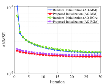
Figure 2: Convergence behavior of the proposed AO-MM and AO-RGA algorithms.

In addition, for a comprehensive performance comparison, the following benchmark schemes are introduced in the simulation: 1) Perfect hardware: We assume perfect hardware implementation in this strategy, i.e. $\beta_{T}\!=\!\beta_{R}\!=\!0$. Moreover, the continuous RIS phase shifts are assumed. Naturally, this system setup characterizes an upper bound on the performance of our considered practical system with hardware impairments. 2) Perfect CSI: The perfect CSI is assumed to be available in this scheme, namely $\sigma_{d}^{2}\!=\!\sigma_{m}^{2}\!=\!0$, while only the hardware distortions are considered. 3) Random phase shift: The discrete phase shift at each RIS element is randomly chosen and kept fixed in the optimization procedure. 4) Identity phase shift: We adopt the identity phase shifting strategy for the RIS optimization. 5) Nonrobust sheme: We adopt the transmit precoder and RIS phase shift design strategy in [11], which neglects the impacts of hardware impairments and channel estimation errors. Due to its continuous phase shift design, we relax the optimal solution to the nearest discrete phase shifts.

To begin with, Fig. 2 shows the convergence behavior of the proposed MM-based AO based algorithm under different initializations, where both the two proposed schemes for optimizing the RIS reflection matrix, as mentioned in Section III.B, are considered. It can be seen from Fig. 2 that both the proposed AO-MM and AO-RGA algorithms under the ideal-based initialization proposed in Algorithm 2 achieve a lower ANMSE than that under the random initialization, which means that the choice of initial points significantly affects the ANMSE performance. This is expected since a good initial point is more likely to lead to a superior solution. In addition, we find that the proposed AO-MM and AO-RGA algorithms can achieve almost the same converged value under each considered initialization. Moreover, these two AO algorithms both converge monotonically within $20$ iterations, which demonstrates their fast convergence speed.

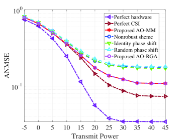
(a) (a) Transmit power

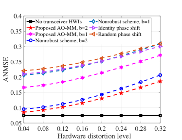
(b) (b) Hardware distoriton

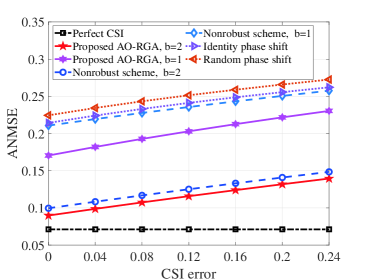
(c) (c) CSI error

Figure 3: ANMSE performance comparison for different algorithms versus (a) the transmit power (b) the hardware distortions (c) the CSI errors.

Next, Fig. 3 shows the ANMSE performance of all studied algorithms versus transmit power, hardware distortion, and CSI error levels. First, Fig. 3 (a) reveals the performance comparison between the proposed algorithms and the benchmark schemes with $b=1$. The perfect hardware and perfect CSI schemes serve as the lower bounds of the proposed MM-based robust designs. It is clear that the perfect hardware scheme performs much better than the perfect CSI scheme, which suggests that the perfect hardware implementation of the transceiver and RIS is much more important than the accurate channel information in the system design. It follows from Fig. 2 that the proposed AO-RGA and AO-MM algorithms are able to achieve almost the same ANMSE performance, both of which outperform the nonrobust scheme in [11]. This is because the nonrobust scheme directly aims at the optimization of the transceiver and RIS reflection matrix under the assumption of perfect CSI and ideal hardware, regardless of the practical non-negligible hardware impairments and CSI errors, which thus leads to an inevitable ANMSE performance loss. We also find that the schemes with random phase shifts and identity phase shifts both perform much worse than the proposed AO-RGA (AO-MM) algorithm with $1$ bit phase shift optimization, thereby demonstrating the necessity of optimizing the RIS reflection matrix and the superiority of the proposed AO algorithms.

Fig. 3 (b) illustrates the ANMSE performance versus hardware distortion level $\beta_{R}$ for different algorithm comparisons, where $\beta_{T}\!=\!0.08$. The scheme of ‘No transceiver HWIs’ considers the perfect transceiver hardware for the RIS-aided MIMO system, which serves as a benchmark. Firstly, it is readily observed that the ANMSE performance decreases with the increasing of hardware distortion level $\beta_{R}$. In addition, as $\beta_{R}$ increases, the performance gap between the proposed MM-based algorithm and the nonrobust algorithm increases, which shows the importance of taking the hardware impairments into consideration. Clearly, both the random phase shift and identity phase shift schemes perform much worse than the proposed algorithm, which highlights the necessity of optimizing the RIS reflection matrix.

In Fig. 3 (c), we also plot the ANMSE performance for algorithms comparison under different CSI errors of the compound channel, i.e. $\sigma_{m}^{2}$, where $\sigma_{d}^{2}\!=\!0.01$. The ‘perfect CSI’ scheme, where only the hardware impairments are considered in the RIS-aided system, acts as a benchmark for other algorithms and keeps constant as the CSI error increases. As the CSI error increases, the system performance of the proposed algorithm and other schemes decreases gradually. Naturally, the nonrobust scheme performs worse than the proposed AO-MM or AO-RGA algorithm, since the impact of the CSI errors is ignored in the system design. It is readily observed that the proposed RIS reflection matrix design can bring huge performance gains compared with the random and identity phase shift schemes, which further demonstrates the effectiveness of the proposed RIS design strategy.

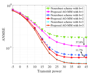
(a) (a) Number of quantization bits

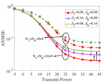
(b) (b) Hardware distoriton

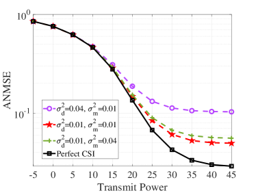
(c) (c) CSI error

Figure 4: ANMSE performance comparison under different system imperfections: (a) the number of quantization bits (b) the hardware distortion levels (c) the CSI errors.

Then, in Fig. 4, we study the impacts of system imperfections, i.e., the number of quantization bits, the transceiver hardware impairments, and the channel estimations errors, on the system ANMSE performance, respectively. To begin with, we compare the proposed AO-MM algorithm with the nonrobust scheme under different number of quantization bits in Fig. 4 (a). Obviously, the performance gap between the proposed AO-MM algorithm and the nonrobust scheme decreases from $37.8\%$ to $11.7\%$ as $b$ increases from 1 to 2, since the RIS phase shifts have more feasible values. This reminds us that using the proposed phase shift design strategy, low-resolution RIS phase shifts can achieve acceptable ANMSE performance in practical hardware implementation. Moreover, we readily find that an irreducible MSE floor exists in the high-SNR regime for each $b$, which is consistent with the theoretical results analyzed in Section IV.B. Obviously, increasing the number of quantization bits will decrease the value of the MSE floor, since the resolution of the RIS phase shifts increases.

Next, Fig. 4 (b) reveals the effect of transceiver hardware distortion on the system ANMSE performance under different Tx-Rx antenna sizes, represented by the dotted line (8x8 MIMO system) and solid line (16x8 MIMO system), respectively. It clearly shows that the ANMSE performance increases correspondingly with the increasing of transmit antenna size. Besides, the MSE floor is also influenced by the level of transceiver hardware impairments. On the other hand, we can readily conclude that when the number of transmit antennas is large than that of receiver antennas, the receiver’s distortion will lead to a more severe impact on the system performance than the transmitter’s distortion. Such influence will be further verified and quantized in the RIS-aided MISO system in Fig. 5. Finally, the impacts of channel estimation errors are illustrated in Fig. 4 (c). From Fig. 4 (c), it is readily inferred that the channel estimation inaccuracy clearly affects the system’s performance and contributes to the performance floor in the high-SNR regime. Moreover, due to the double path loss effect of the RIS-related compound channels, the channel estimation inaccuracy of the direct channel induces a more severe influence on the system performance than the compound channels.

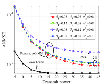
Figure 5: ANMSE performance versus transmit power under different system parameter setups in the RIS-aided MISO system.

In order to validate the theoretical analysis in Section IV.B, Fig. 5 shows the ANMSE performance of the proposed AO-MM algorithm versus the transmit power $P$ for the RIS-aided MISO system, where $N_{T}\!=\!8$, $N_{R}\!=d\!=\!1$. Firstly, it can be seen that the performance of the proposed algorithm is lower bounded by $f_{\rm lower}^{\rm opt}$ mentioned in Proposition 1, which is denoted as ‘Lower bound’ in Fig. 5, for each SNR. Note that the hardware distortions at the transmitter’s and receiver’s sides have different impacts on the system performance in the RIS-aided MISO case. Specifically, the receiver distortion, i.e. $\beta_{R}$, causes more severe performance loss, about $70\%$, than transmitter distortion $\beta_{T}$, when the distortion level changes from 0.08 to 0.12. This reminds us that more expensive hardware should be deployed on the user’s side rather than the BS’s side. In addition, increasing the CSI errors of the compound channel, i.e. $\sigma_{m}^{2}$, also increases the MSE floor. Therefore, combining the results of Fig. 4 and Fig. 5, we conclude that the transceiver hardware distortions, CSI errors, and RIS phase noise all lead to the irreducible MSE floor in the RIS-aided MIMO/MISO communication system.

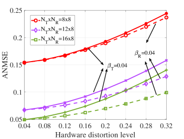
(a) (a) Tx-Rx sizes

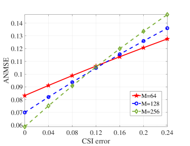
(b) (b) RIS elements

Figure 6: ANMSE performance versus the system imperfections under different number of (a) Tx-Rx sizes (b) RIS elements.

In Fig. 6, the ANMSE performance versus the channel estimation errors and transceiver hardware impairments under different numbers of transmitter’s antennas and RIS elements has been investigated. First, Fig. 6 (a) shows the system’s performance versus the hardware distortion level $\beta_{T}$ or $\beta_{R}$ for different Tx-Rx configurations, represented by the dotted line and solid line, respectively. It is evident that as the size of the transmitter antenna increases, the performance gap brought by the transmitter’s and receiver’s distortion increases, which further demonstrates that the user’s hardware has more impact in the system performance than that at BS in realistic communications. Besides, it can be seen from Fig. 6 (b) that the ANMSE performance increases as the number of RIS elements $M$ increases for a small region $0\thicksim 0.12$. The reason is that the RIS benefits from the diversity gain by increasing number of RIS elements. However, in the high CSI error regime, increasing the number of RIS elements may decrease the ANMSE performance, since the impact induced by imperfect RIS-related channels dominates the diversity gain. As such, we readily conclude that cares must be taken w.r.t. the size of RIS in enhancing the system’s performance.

VI conclusion

In this work, we studied the robust transceiver and passive beamforming design for the RIS-aided MIMO system with the existence of hardware impairments at the transceiver and RIS and channel errors. We aimed to minimize the total average MSE for all data streams subject to the total power constraint at BS and discrete phase constraints at RIS. To tackle this non-convex NP-hard optimization problem, an efficient AO-based algorithm was proposed. Moreover, to handle the non-convex discrete phase constraints, we also proposed two methods, namely two-tier MM-based algorithm and modified RGA method, to obtain the sub-optimal solution of the RIS reflection matrix. Futhermore, we also studied the special cases of RIS-aided MIMO system, e.g., RIS-aided MIMO system without direct link and RIS-aided MISO system, to demonstrate the optimality of the proposed algorithm and the MSE performance floor in the high-SNR regime, respectively. Simulation results demonstrated the superiority of our proposed algorithms compared to the nonrobust design and other benchmark schemes. It was also found that increasing the number of RIS elements was not always beneficial under severe CSI errors. These results provided useful insights for the implementation of practical RIS-aided MIMO systems.

Appendix A

Recalling the lower bound of $f_{\rm MSE}({{\bf{w}},{\bm{\theta}}})$ in (IV-B), the transmit precoder design for $f_{\rm lower}({{\bf{w}},{\bm{\theta}}})$ is equivalently transformed into the the maximization of a generalized Rayleigh quotient as

$$(\text{P9}):\ \max_{{\bf{w}}}\quad \frac{{\bf w}^{H}{\bf{\bar{h}}}{\bf{\bar{h}}}^{H}{\bf w}}{{\bf w}^{H}\left(\frac{c_{2}}{P}(1\!\!+\!\!\beta_{T}^{2}){\bf I}\!\!+\!\!(1\!\!+\!\!\beta_{R}^{2}){\bf{\bar{h}}}{\bf{\bar{h}}}^{H}\!\!+\!\!{\bf Q}\right){\bf w}}$$

s.t. $$(1\!+\!\beta_{T}^{2})||{\bf{w}}||^{2}\leq P,$$ (42)

where ${\bf{Q}}$ has been defined in Proposition 1. Hence, the optimal transmit precoder ${\bf w}^{\star}$ can be derived as

$${\bf w}^{\star}\!\!=\!\!\sqrt{\frac{P}{1\!\!+\!\!\beta_{T}^{2}}}\frac{(\frac{c_{2}}{P}(1\!\!+\!\!\beta_{T}^{2}){\bf I}\!+\!(1\!+\!\beta_{R}^{2}){\bf{\bar{h}}}{\bf{\bar{h}}}^{H}\!+\!{\bf Q})^{-1}{\bf{\bar{h}}}}{\left\lVert(\frac{c_{2}}{P}(1+\beta_{T}^{2}){\bf I}\!+\!(1\!+\!\beta_{R}^{2}){\bf{\bar{h}}}{\bf{\bar{h}}}^{H}\!+\!{\bf Q})^{-1}{\bf{\bar{h}}}\right\rVert}.$$ (43)

By substituting the optimal ${\bf w}^{\star}$ and relaxing the unit-modulus discrete phase constraints of (10c), the optimization problem for the RIS reflection beamforming is further given by

$$(\text{P10}):\max_{{\bm{\theta}}}\ \frac{{\bm{\tilde{\theta}}}^{H}{\bf{\tilde{H}}}_{\rm cat}^{H}({\bf{Q}}\!+\!(1\!+\!\beta_{T}^{2})\frac{\sigma^{2}}{P}{\bf{I}}_{N_{T}})^{-1}{\bf{\tilde{H}}}_{\rm cat}{\bm{\tilde{\theta}}}}{1\!\!+\!\!(1\!\!+\!\!\beta_{R}^{2}){\bm{\tilde{\theta}}}^{H}{\bf{\tilde{H}}}_{\rm cat}^{H}({\bf{Q}}\!\!+\!\!(1\!\!+\!\!\beta_{T}^{2})\frac{\sigma^{2}}{P}{\bf{I}}_{N_{T}})^{-1}{\bf{\tilde{H}}}_{\rm cat}{\bm{\tilde{\theta}}}},$$

s.t. $$||{\bm{\tilde{\theta}}}||_{2}^{2}\leq M+1,$$ (44)

where ${\bf{\tilde{H}}}_{\rm cat}$ is defined in Proposition 1. Note that the objective function in Problem (P10) is monotonically increasing with the term of ${{{\bm{\tilde{\theta}}}^{H}{\bf{\tilde{H}}}_{\rm cat}^{H}({\bf{Q}}\!+\!(1\!+\!\beta_{T}^{2})\frac{\sigma^{2}}{P}{\bf{I}}_{N_{T}})^{-1}{\bf{\tilde{H}}}_{\rm cat}{\bm{\tilde{\theta}}}}}$. Therefore, the problem (P10) for the RIS phase shift design can be equivalently transformed to the maximization of ${{\bm{\tilde{\theta}}}^{H}{\bf{\tilde{H}}}_{\rm cat}^{H}({\bf{Q}}\!+\!(1\!+\!\beta_{T}^{2})\frac{\sigma^{2}}{P}{\bf{I}}_{N_{T}})^{-1}{\bf{\tilde{H}}}_{\rm cat}{\bm{\tilde{\theta}}}}$. It is readily inferred that maximum value can be obtained as $(M\!+\!1)\lambda_{\rm max}({\bf{\tilde{H}}}_{\rm cat}^{H}({\bf{Q}}\!+\!(1\!+\!\beta_{T}^{2})\frac{\sigma^{2}}{P}{\bf{I}}_{N_{T}})^{-1}{\bf{\tilde{H}}}_{\rm cat})$ when ${\bm{\theta}}\!=\!\sqrt{(M+1)}{\bf u}_{\rm max}$ by leveraging the Cauchy-Schwarz inequality, where ${\bf u}_{\rm max}$ denotes the corresponding eigenvector w.r.t the largest eigenvalue $\lambda_{\rm max}$ from the EVD of ${\bf{\tilde{H}}}_{\rm cat}^{H}({\bf{Q}}\!+\!(1\!+\!\beta_{T}^{2})\frac{\sigma^{2}}{P}{\bf{I}}_{N_{T}})^{-1}{\bf{\tilde{H}}}_{\rm cat}$. Based on the above transformation and relaxation, the optimal value of $f_{\rm lower}({{\bf{w}},{\bm{\theta}}})$ is lower bounded by

$$f_{\rm lower}^{\rm opt}=$$

$$\!\!1\!\!-\!\!\frac{(M+1)\lambda_{\rm max}({\bf{\tilde{H}}}_{\rm cat}^{H}({\bf{Q}}\!+\!(1\!+\!\beta_{T}^{2})\frac{\sigma^{2}}{P}{\bf{I}}_{N_{T}})^{-1}{\bf{\tilde{H}}}_{\rm cat})}{1\!\!+\!\!(1\!\!+\!\!\beta_{R}^{2})(M\!\!+\!\!1)\lambda_{\rm max}({\bf{\tilde{H}}}_{\rm cat}^{H}({\bf{Q}}\!\!+\!\!(1\!\!+\!\!\beta_{T}^{2})\frac{\sigma^{2}}{P}{\bf{I}}_{N_{T}})^{-1}{\bf{\tilde{H}}}_{\rm cat})}.$$ (45)

Moreover, in the high-SNR regime, i.e. $\frac{P}{\sigma^{2}}\to\infty$, the optimal value of $f_{\rm lower}^{\rm opt}$ is reduced to the MSE floor, expressed as

$$f_{\rm floor}=1-\frac{(M+1)\lambda_{\rm max}({\bf{\tilde{H}}}_{\rm cat}^{H}{\bf{Q}}^{-1}{\bf{\tilde{H}}}_{\rm cat})}{1\!+\!(1\!+\!\beta_{R}^{2})(M\!+\!1)\lambda_{\rm max}({\bf{\tilde{H}}}_{\rm cat}^{H}{\bf{Q}}^{-1}{\bf{\tilde{H}}}_{\rm cat})}.$$ (46)

Thus, we complete the proof.

Appendix B

To begin with, we generally characterize the relationship between surrogate function $g({\bf x};{\bf x}_{t})$ and original function $f({\bf x})$ in the MM technique. For any iteration, $g({\bf x};{\bf x}_{t})$ is the majoring function of $f({\bf x})$ at ${\bf x}_{t}$, which satisfies 1) $g({\bf x};{\bf x}_{t})\leq f({\bf x}),\forall{\bf x}\in{\rm dom}f$ 2) $g({\bf x}_{t};{\bf x}_{t})=f({\bf x}_{t})$, 3) $\nabla_{{\bf x}}g({\bf x};{\bf x}_{t})|_{{\bf x}={\bf x}_{t}}=\nabla_{{\bf x}}f({\bf x})$, 4) $g({\bf x};{\bf x}_{t})$ is continuous in both ${\bf x}$ and ${\bf x}_{t}$. The first two conditions guarantee $g({\bf x};{\bf x}_{t})$ is a tight global lower bound of $f({\bf x})$, while the last two conditions guarantee convergence to a stationary solution. Recalling the surrogate function defined in (13), (20) and (23), it is easily verified that they all satisfy these four conditions.

Specifically, in the optimization of the transmit precoder with RIS reflection matrix fixed at the $t$-th iteration, we have

$${g_{\rm sub1}^{\rm Low}({\bf{W}};{\bf W}_{t}|{\bm{\theta}}_{t})}\leq g_{\rm MSE}({\bf{W}},{\bm{\theta}}_{t}),$$ (47a)

$${g_{\rm sub1}^{\rm Low}({\bf{W}}_{t};{\bf W}_{t}|{\bm{\theta}}_{t})}=g_{\rm MSE}({\bf{W}}_{t},{\bm{\theta}}_{t}).$$ (47b)

The update rule for the transmit precoder as proposed in Section III.A can be rewritten as

$${\bf{W}}_{t+1}={\rm arg}\max_{{\bf{W}}}{g_{\rm sub1}^{\rm Low}({\bf{W}};{\bf W}_{t})}$$ (48)

where the closed form has been derived in (17). Hence, the following relationship between the objective values holds:

$$g_{\rm MSE}({\bf{W}}_{t},{\bm{\theta}}_{t}) \mathop{=}\limits^{({d_{1}})}{g_{\rm sub1}^{\rm Low}({\bf{W}}_{t};{\bf W}_{t}|{\bm{\theta}}_{t})}$$

$$\mathop{\leq}\limits^{({d_{2}})}{g_{\rm sub1}^{\rm Low}({\bf{W}}_{t+1};{\bf W}_{t},{\bm{\theta}}_{t})}$$

$$\mathop{\leq}\limits^{({d_{3}})}g_{\rm MSE}({\bf{W}}_{t+1},{\bm{\theta}}_{t})$$ (49)

where $(d_{1})$ holds because of (47b), $(d_{2})$ holds since (48) is optimally solved and $(d_{3})$ is due to (47a).

In the optimization of the passive RIS using the two-tier MM-based algorithm with transmit precoder fixed, we have

$${g_{\rm sub2}^{\rm Low}({\bm{\theta}};{\bm{\theta}}_{t}|{\bf W}_{t}})\leq g_{\rm MSE}({\bf{W}}_{t},{\bm{\theta}}),$$ (50a)

$${g_{\rm sub2}^{\rm Low}({\bm{\theta}}_{t};{\bm{\theta}}_{t}|{\bf W}_{t})}=g_{\rm MSE}({\bf{W}}_{t},{\bm{\theta}}_{t}),$$ (50b)

$${{\tilde{g}}_{\rm sub2}^{\rm Low}({\bm{\theta}};{\bm{\theta}}_{t,r}|{\bf W}_{t})}\leq{g_{\rm sub2}^{\rm Low}({\bm{\theta}};{\bm{\theta}}_{t}|{\bf W}_{t})},$$ (50c)

$${{\tilde{g}}_{\rm sub2}^{\rm Low}({\bm{\theta}}_{t,r};{\bm{\theta}}_{t,r}|{\bf W}_{t})}={g_{\rm sub2}^{\rm Low}({\bm{\theta}}_{t,r};{\bm{\theta}}_{t}|{\bf W}_{t})},$$ (50d)

where $r$ denotes the $r$-th iteration for updating ${\bm{\theta}}$ using the MM technique. Denoting the maximum number of iteration as $R$, we have ${\bm{\theta}}_{t,0}\!=\!{\bm{\theta}}_{t}$ and ${\bm{\theta}}_{t,R-1}\!=\!{\bm{\theta}}_{t+1}$. The update rule for the passive RIS in the two-tier MM-based algorithm is re-expressed as

$${\bm{\theta}}_{t,r+1}={\rm arg}\max_{{\bm{\theta}}}~{}{{\tilde{g}}_{\rm sub2}^{\rm Low}({\bm{\theta}};{\bm{\theta}}_{t,r}|{\bf W}_{t})},$$ (51)

which is essentially defined as (25). Then, the following relationship holds:

$$g_{\rm MSE}({\bf{W}}_{t+1},{\bm{\theta}}_{t})$$

$$\mathop{=}\limits^{({e_{1}})}{g_{\rm sub2}^{\rm Low}({\bm{\theta}}_{t};{\bm{\theta}}_{t}|{\bf W}_{t+1})}\mathop{=}\limits^{({e_{2}})}{{\tilde{g}}_{\rm sub2}^{\rm Low}({\bm{\theta}}_{t,0};{\bm{\theta}}_{t,0}|{\bf W}_{t+1})}$$

$$\mathop{\leq}\limits^{({e_{3}})}{{\tilde{g}}_{\rm sub2}^{\rm Low}({\bm{\theta}}_{t+1};{\bm{\theta}}_{t,R-2}|{\bf W}_{t+1})}\mathop{\leq}\limits^{({e_{4}})}{g_{\rm sub2}^{\rm Low}({\bm{\theta}}_{t+1};{\bm{\theta}}_{t}|{\bf W}_{t+1})}$$

$$\mathop{\leq}\limits^{({e_{5}})}g_{\rm MSE}({\bf{W}}_{t+1},{\bm{\theta}}_{t+1}),$$ (52)

where $(e_{1})$ and $(e_{2})$ hold due to the properties of (50b) and (50d), respectively. $(e_{3})$ holds because of the update rule in (51), $(e_{4})$ is due to the equation in (50c), and $(e_{5})$ follows (50a).

Similarly, in the optimization of the passive RIS using the modified RGA algorithm, the relationship of (50a) and (50b) still hold. However, the update rule is conducted by the Riemannian gradient ascent on the CCM space, and can be rewritten as

$${\bm{\theta}}_{t+1}={\rm arg}\max_{{\bm{\theta}}}~{}{{g}_{\rm sub2}^{\rm Low}({\bm{\theta}};{\bm{\theta}}_{t}|{\bf W}_{t})},$$ (53)

where the monotonicity is guaranteed by the backtracking search method. Thus, we have the following relationship:

$$g_{\rm MSE}({\bf{W}}_{t+1},{\bm{\theta}}_{t}) \mathop{=}\limits^{({f_{1}})}{g_{\rm sub2}^{\rm Low}({\bm{\theta}}_{t};{\bm{\theta}}_{t}|{\bf W}_{t+1})}$$

$$\mathop{\leq}\limits^{({f_{2}})}{g_{\rm sub2}^{\rm Low}({\bm{\theta}}_{t+1};{\bm{\theta}}_{t}|{\bf W}_{t+1})}$$

$$\mathop{\leq}\limits^{({f_{3}})}\!g_{\rm MSE}({\bf{W}}_{t+1},{\bm{\theta}}_{t+1}),$$ (54)

where $(f_{1})$ holds due to (50b), $(f_{2})$ holds since (53) is optimally solved and $(f_{3})$ is because of (50a). Therefore, with the fact of (B) and (52) (54), the objective value $g_{\rm MSE}({\bf{W}},{\bm{\theta}})$ is monotonically non-decreasing in the proposed AO-MM or AO-RGA algorithm and finally converges to a finite value due to it is bounded. Thus, we complete the proof for Proposition 2.

Jintao Wang received the B.S. degree in 2020 in communication engineering from Jilin University, Changchun, China. He is currently pursuing the Ph.D. degree with the State Key Laboratory of Internet of Things for Smart City and the Department of Electrical and Computer Engineering, University of Macau, Macau, China. His main research interests include RIS-aided communication, mmWave communication, transceiver design and convex optimization.

Shiqi Gong received the B.S. and Ph.D. degrees in electronic engineering from Beijing Institute of Technology, China, in 2014 and 2020, respectively. From January 2021 to August 2022, she was a postdoctoral fellow with the State Key Laboratory of Internet of Things for Smart City, University of Macau, China. She is currently an associate professor with the School of Cyberspace Science and Technology, Beijing Institute of Technology. Her research interests are in the areas of signal processing, mmWave and Terahertz communications and convex optimization. She was a recipient of the Best Ph.D. Thesis Award of Beijing Institute of Technology in 2020.

Qingqing Wu (S’13-M’16-SM’21) received the B.Eng. and the Ph.D. degrees in Electronic Engineering from South China University of Technology and Shanghai Jiao Tong University (SJTU) in 2012 and 2016, respectively. From 2016 to 2020, he was a Research Fellow in the Department of Electrical and Computer Engineering at National University of Singapore. He is currently an Associate Professor with Shanghai Jiao Tong University. His current research interest includes intelligent reflecting surface (IRS), unmanned aerial vehicle (UAV) communications, and MIMO transceiver design. He has coauthored more than 100 IEEE journal papers with 26 ESI highly cited papers and 8 ESI hot papers, which have received more than 18,000 Google citations. He was listed as the Clarivate ESI Highly Cited Researcher in 2022 and 2021, the Most Influential Scholar Award in AI-2000 by Aminer in 2021 and World’s Top 2% Scientist by Stanford University in 2020 and 2021. He was the recipient of the IEEE Communications Society Asia Pacific Best Young Researcher Award and Outstanding Paper Award in 2022, the IEEE Communications Society Young Author Best Paper Award in 2021, the Outstanding Ph.D. Thesis Award of China Institute of Communications in 2017, the Outstanding Ph.D. Thesis Funding in SJTU in 2016, the IEEE ICCC Best Paper Award in 2021, and IEEE WCSP Best Paper Award in 2015. He was the Exemplary Editor of IEEE Communications Letters in 2019 and the Exemplary Reviewer of several IEEE journals. He serves as an Associate Editor for IEEE Transactions on Communications, IEEE Communications Letters, IEEE Wireless Communications Letters, IEEE Open Journal of Communications Society (OJ-COMS), and IEEE Open Journal of Vehicular Technology (OJVT). He is the Lead Guest Editor for IEEE Journal on Selected Areas in Communications on “UAV Communications in 5G and Beyond Networks”, and the Guest Editor for IEEE OJVT on “6G Intelligent Communications” and IEEE OJ-COMS on “Reconfigurable Intelligent Surface-Based Communications for 6G Wireless Networks”. He is the workshop co-chair for IEEE ICC 2019-2022 workshop on “Integrating UAVs into 5G and Beyond”, and the workshop co-chair for IEEE GLOBECOM 2020 and ICC 2021 workshop on “Reconfigurable Intelligent Surfaces for Wireless Communication for Beyond 5G”. He serves as the Workshops and Symposia Officer of Reconfigurable Intelligent Surfaces Emerging Technology Initiative and Research Blog Officer of Aerial Communications Emerging Technology Initiative. He is the IEEE Communications Society Young Professional Chair in Asia Pacific Region.

Shaodan Ma (Senior Member, IEEE) received the double Bachelor’s degrees in science and economics and the M.Eng. degree in electronic engineering from Nankai University, Tianjin, China, in 1999 and 2002, respectively, and the Ph.D. degree in electrical and electronic engineering from The University of Hong Kong, Hong Kong, in 2006. From 2006 to 2011, she was a post-doctoral fellow at The University of Hong Kong. Since August 2011, she has been with the University of Macau, where she is currently a Professor. Her research interests include array signal processing, transceiver design, localization, mmWave communications and massive MIMO. She was a symposium co-chair for various conferences including IEEE ICC 2021, 2019 and 2016, IEEE/CIC ICCC 2019, IEEE GLOBECOM 2016, etc. Currently she serves as an Editor for IEEE Transactions on Wireless Communications, IEEE Transactions on Communications, IEEE Communications Letters, and Journal of Communications and Information Networks.

References

- [1] S. Li, B. Duo, M. D. Renzo, M. Tao, and X. Yuan, “Robust secure UAV communications with the aid of reconfigurable intelligent surfaces,” IEEE Trans. Wireless Commun., vol. 20, no. 10, pp. 6402–6417, 2021.
- [2] H. Du, J. Zhang, J. Cheng, and B. Ai, “Millimeter wave communications with reconfigurable intelligent surfaces: Performance analysis and optimization,” IEEE Trans. Commun., vol. 69, no. 4, pp. 2752–2768, 2021.
- [3] S. Hong, C. Pan, H. Ren, K. Wang, K. K. Chai, and A. Nallanathan, “Robust transmission design for intelligent reflecting surface-aided secure communication systems with imperfect cascaded CSI,” IEEE Trans. Wireless Commun., vol. 20, no. 4, pp. 2487–2501, 2021.
- [4] H. Yang, X. Yuan, J. Fang, and Y.-C. Liang, “Reconfigurable intelligent surface aided constant-envelope wireless power transfer,” IEEE Trans. Signal Process., vol. 69, pp. 1347–1361, 2021.
- [5] Q. Wu, S. Zhang, B. Zheng, C. You, and R. Zhang, “Intelligent reflecting surface aided wireless communications: A tutorial,” IEEE Trans. Commun., 2021.
- [6] Q. Wu and R. Zhang, “Intelligent reflecting surface enhanced wireless network via joint active and passive beamforming,” IEEE Trans. Wireless Commun., vol. 18, no. 11, pp. 5394–5409, 2019.
- [7] Z. Yang, W. Xu, C. Huang, J. Shi, and M. Shikh-Bahaei, “Beamforming design for multiuser transmission through reconfigurable intelligent surface,” IEEE Trans. Commun., vol. 69, no. 1, pp. 589–601, 2021.
- [8] C. Pan, H. Ren, K. Wang, W. Xu, M. Elkashlan, A. Nallanathan, and L. Hanzo, “Multicell MIMO communications relying on intelligent reflecting surfaces,” IEEE Trans. Wireless Commun., vol. 19, no. 8, pp. 5218–5233, 2020.
- [9] K. Xu, J. Zhang, X. Yang, S. Ma, and G. Yang, “On the sum-rate of RIS-assisted MIMO multiple-access channels over spatially correlated rician fading,” IEEE Trans. Commun., vol. 69, no. 12, pp. 8228–8241, 2021.
- [10] J. Zhang, J. Liu, S. Ma, C.-K. Wen, and S. Jin, “Large system achievable rate analysis of RIS-assisted MIMO wireless communication with statistical CSIT,” IEEE Trans. Wireless Commun., vol. 20, no. 9, pp. 5572–5585, 2021.
- [11] X. Zhao, K. Xu, S. Ma, S. Gong, G. Yang, and C. Xing, “Joint transceiver optimization for IRS-aided MIMO communications,” IEEE Trans. Commun., vol. 70, no. 5, pp. 3467–3482, 2022.
- [12] S. Gong, C. Xing, X. Zhao, S. Ma, and J. An, “Unified IRS-aided MIMO transceiver designs via majorization theory,” IEEE Trans. Signal Process., vol. 69, pp. 3016–3032, 2021.
- [13] K. Xu, S. Gong, M. Cui, G. Zhang, and S. Ma, “Statistically robust transceiver design for multi-RIS assisted multi-user MIMO systems,” IEEE Commun. Lett., vol. 26, no. 6, pp. 1428–1432, 2022.
- [14] L. You, J. Xiong, D. W. K. Ng, C. Yuen, W. Wang, and X. Gao, “Energy efficiency and spectral efficiency tradeoff in RIS-aided multiuser MIMO uplink transmission,” IEEE Trans. Signal Process., vol. 69, pp. 1407–1421, 2021.
- [15] C. Huang, A. Zappone, G. C. Alexandropoulos, M. Debbah, and C. Yuen, “Reconfigurable intelligent surfaces for energy efficiency in wireless communication,” IEEE Trans. Wireless Commun., vol. 18, no. 8, pp. 4157–4170, 2019.
- [16] S. Gong, Z. Yang, C. Xing, J. An, and L. Hanzo, “Beamforming optimization for intelligent reflecting surface-aided SWIPT IoT networks relying on discrete phase shifts,” IEEE Internet Things J., vol. 8, no. 10, pp. 8585–8602, 2020.
- [17] M. Hua, Q. Wu, D. W. K. Ng, J. Zhao, and L. Yang, “Intelligent reflecting surface-aided joint processing coordinated multipoint transmission,” IEEE Trans. Commun., vol. 69, no. 3, pp. 1650–1665, 2021.
- [18] Z. He, H. Shen, W. Xu, and C. Zhao, “Low-cost passive beamforming for RIS-aided wideband OFDM systems,” IEEE Wireless Commun. Lett., vol. 11, no. 2, pp. 318–322, 2022.
- [19] Y. Yang, B. Zheng, S. Zhang, and R. Zhang, “Intelligent reflecting surface meets OFDM: Protocol design and rate maximization,” IEEE Trans. Commun., vol. 68, no. 7, pp. 4522–4535, 2020.
- [20] C. Pradhan, A. Li, L. Song, J. Li, B. Vucetic, and Y. Li, “Reconfigurable intelligent surface (RIS)-enhanced two-way OFDM communications,” IEEE Trans. Veh. Technol., vol. 69, no. 12, pp. 16 270–16 275, 2020.
- [21] T. Schenk, RF Imperfections in High-rate Wireless Systems. Springer, Dordrecht, 2008.
- [22] J. Feng, S. Ma, S. Aïssa, and M. Xia, “Two-way massive MIMO relaying systems with non-ideal transceivers: Joint power and hardware scaling,” IEEE Trans. Commun., vol. 67, no. 12, pp. 8273–8289, 2019.
- [23] C. Studer, M. Wenk, and A. Burg, “MIMO transmission with residual transmit-RF impairments,” in Proc. Int. ITG Workshop Smart Antennas (WSA), Bremen, Germany, Feb. 2010, pp. 189–196.
- [24] A.-A. A. Boulogeorgos and A. Alexiou, “How much do hardware imperfections affect the performance of reconfigurable intelligent surface-assisted systems?” IEEE Open J. Commun. Soc., vol. 1, pp. 1185–1195, 2020.
- [25] A. M. T. Khel and K. A. Hamdi, “Effects of hardware impairments on IRS-enabled MISO wireless communication systems,” IEEE Commun. Lett., vol. 26, no. 2, pp. 259–263, 2021.
- [26] M. A. Saeidi, M. J. Emadi, H. Masoumi, M. R. Mili, D. W. K. Ng, and I. Krikidis, “Weighted sum-rate maximization for multi-IRS-assisted full-duplex systems with hardware impairments,” IEEE Trans. Cogn. Commun. Netw., vol. 7, no. 2, pp. 466–481, 2021.
- [27] G. Zhou, C. Pan, H. Ren, K. Wang, and Z. Peng, “Secure wireless communication in RIS-aided MISO system with hardware impairments,” IEEE Wireless Commun. Lett., vol. 10, no. 6, pp. 1309–1313, 2021.
- [28] H. Shen, W. Xu, S. Gong, C. Zhao, and D. W. K. Ng, “Beamforming optimization for IRS-aided communications with transceiver hardware impairments,” IEEE Trans. Commun., vol. 69, no. 2, pp. 1214–1227, 2021.
- [29] S. Zhou, W. Xu, K. Wang, M. Di Renzo, and M.-S. Alouini, “Spectral and energy efficiency of IRS-assisted MISO communication with hardware impairments,” IEEE Wireless Commun. Lett., vol. 9, no. 9, pp. 1366–1369, 2020.
- [30] M.-A. Badiu and J. P. Coon, “Communication through a large reflecting surface with phase errors,” IEEE Wireless Commun. Lett., vol. 9, no. 2, pp. 184–188, 2020.
- [31] J. Zhao, M. Chen, C. Pan, Z. Li, G. Zhou, and X. Chen, “MSE-based transceiver designs for RIS-aided communications with hardware impairments,” IEEE Commun. Lett., pp. 1–1, 2022.
- [32] Y. Liu, E. Liu, and R. Wang, “Energy efficiency analysis of intelligent reflecting surface system with hardware impairments,” in Proc. IEEE Global Commun. Conf. (GLOBECOM), Taipei, Taiwan, 2020, pp. 1–6.
- [33] Z. Xing, R. Wang, J. Wu, and E. Liu, “Achievable rate analysis and phase shift optimization on intelligent reflecting surface with hardware impairments,” IEEE Trans. Wireless Commun., vol. 20, no. 9, pp. 5514–5530, 2021.
- [34] Z. Chu, J. Zhong, P. Xiao, D. Mi, W. Hao, R. Tafazolli, and A. P. Feresidis, “RIS assisted wireless powered IoT networks with phase shift error and transceiver hardware impairment,” IEEE Trans. Commun., vol. 70, no. 7, pp. 4910–4924, 2022.
- [35] J. Dai, F. Zhu, C. Pan, H. Ren, and K. Wang, “Statistical CSI-based transmission design for reconfigurable intelligent surface-aided massive MIMO systems with hardware impairments,” IEEE Wireless Commun. Lett., pp. 1–1, 2021.
- [36] Z. Peng, Z. Chen, C. Pan, G. Zhou, and H. Ren, “Robust transmission design for RIS-aided communications with both transceiver hardware impairments and imperfect CSI,” IEEE Wireless Commun. Lett., vol. 11, no. 3, pp. 528–532, 2022.
- [37] Y. Liu, E. Liu, and R. Wang, “Beamforming and performance evaluation for intelligent reflecting surface aided wireless system with hardware impairments,” arXiv preprint arXiv:2006.00664, 2020.
- [38] A. Papazafeiropoulos, C. Pan, P. Kourtessis, S. Chatzinotas, and J. M. Senior, “Intelligent reflecting surface-assisted MU-MISO systems with imperfect hardware: Channel estimation and beamforming design,” IEEE Trans. Wireless Commun., vol. 21, no. 3, pp. 2077–2092, 2021.
- [39] C. Xing, S. Wang, S. Chen, S. Ma, H. V. Poor, and L. Hanzo, “Matrix-monotonic optimization-Part I: Single-variable optimization,” IEEE Trans. Signal Process., vol. 69, pp. 738–754, 2021.
- [40] O. Y. Kolawole, S. Biswas, K. Singh, and T. Ratnarajah, “Transceiver design for energy-efficiency maximization in mmwave MIMO IoT networks,” IEEE Trans. Green Commun. Netw., vol. 4, no. 1, pp. 109–123, 2020.
- [41] E. Bjornson, P. Zetterberg, M. Bengtsson, and B. Ottersten, “Capacity limits and multiplexing gains of MIMO channels with transceiver impairments,” IEEE Commun. Lett., vol. 17, no. 1, pp. 91–94, 2013.
- [42] X. Wu, S. Ma, and X. Yang, “Tensor-based low-complexity channel estimation for mmwave massive MIMO-OTFS systems,” J. Commun. Netw., vol. 5, no. 3, pp. 324–334, 2020.
- [43] C. You, B. Zheng, and R. Zhang, “Intelligent reflecting surface with discrete phase shifts: Channel estimation and passive beamforming,” in ICC 2020 - 2020 IEEE Int. Conf. Commun. (ICC), pp. 1–6.
- [44] K.-Y. Wang, A. M.-C. So, T.-H. Chang, W.-K. Ma, and C.-Y. Chi, “Outage constrained robust transmit optimization for multiuser MISO downlinks: Tractable approximations by conic optimization,” IEEE Trans. Signal Process., vol. 62, no. 21, pp. 5690–5705, 2014.
- [45] J. Zhang, Y. Zhang, C. Zhong, and Z. Zhang, “Robust design for intelligent reflecting surfaces assisted MISO systems,” IEEE Commun. Lett., vol. 24, no. 10, pp. 2353–2357, 2020.
- [46] Y. Sun, P. Babu, and D. P. Palomar, “Majorization-minimization algorithms in signal processing, communications, and machine learning,” IEEE Trans. Signal Process., vol. 65, no. 3, pp. 794–816, 2017.
- [47] K. Alhujaili, V. Monga, and M. Rangaswamy, “Transmit MIMO radar beampattern design via optimization on the complex circle manifold,” IEEE Trans. Signal Process., vol. 67, no. 13, pp. 3561–3575, 2019.
- [48] Y. S. Cho, J. Kim, W. Y. Yang, and C. G. Kang, MIMO-OFDM wireless communications with MATLAB. John Wiley & Sons, 2010.
- [49] X. Zhang, M. Matthaiou, E. Björnson, M. Coldrey, and M. Debbah, “On the MIMO capacity with residual transceiver hardware impairments,” in 2014 IEEE Int. Conf. Commun. (ICC), pp. 5299–5305.
- [50] E. Björnson, J. Hoydis, M. Kountouris, and M. Debbah, “Massive MIMO systems with non-ideal hardware: Energy efficiency, estimation, and capacity limits,” IEEE Trans. Inf. Theory, vol. 60, no. 11, pp. 7112–7139, 2014.
- [51] H. Holma and A. Toskala, LTE for UMTS: Evolution to LTE-advanced. John Wiley & Sons, 2011.