Dynamical quantum phase transitions in a spinor Bose-Einstein condensate and criticality enhanced quantum sensing

Abstract

Quantum phase transitions universally exist in the ground and excited states of quantum many-body systems, and they have a close relationship with the nonequilibrium dynamical phase transitions, which however are challenging to identify. In the system of spin-1 Bose-Einstein condensates, though dynamical phase transitions with correspondence to equilibrium phase transitions in the ground state and uppermost excited state have been probed, those taken place in intermediate excited states remain untouched in experiments thus far. Here we unravel that both the ground and excited-state quantum phase transitions in spinor condensates can be diagnosed with dynamical phase transitions. A connection between equilibrium phase transitions and nonequilibrium behaviors of the system is disclosed in terms of the quantum Fisher information. We also demonstrate that near the critical points parameter estimation beyond standard quantum limit can be implemented. This work not only advances the exploration of excited-state quantum phase transitions via a scheme that can immediately be applied to a broad class of few-mode quantum systems, but also provides new perspective on the relationship between quantum criticality and quantum enhanced sensing.

Introduction.—In quantum many-body systems, excited-state quantum phase transitions (ESQPTs) can be more appealing compared with quantum phase transitions (QPTs), which refer to quantum criticality aroused in ground states Sachdev (2000). ESQPTs extend the study of criticality to excitation spectra and have recently been disclosed in several quantum systems Cejnar et al. (2021, 2006); Caprio et al. (2008); Corps and Relaño (2021); Lipkin et al. (1965); Ulyanov and Zaslavskii (1992). The criticalities associated with QPTs and ESQPTs can reveal themselves by nonequilibrium quantum phenomena, especially dynamical phase transition (DPT) Heyl et al. (2013); Heyl (2015, 2019); De Nicola et al. (2021); Vajna and Dóra (2015); Jurcevic et al. (2017); Yang et al. (2019a); Guo et al. (2019); Lang et al. (2018); Fläschner et al. (2018); Zhang et al. (2017); Muniz et al. (2020).

DPT is characteristic of the nonanalyticity in the Loschmidt echo rate function after quantum quench. More experimentally accessible clue would be that physical quantities become nonanalytical as a function of time, such as the order parameter. It is still an open question on the universal correspondence between DPTs and QPTs, also ESQPTs.

In this work, taking the system of an antiferromagnetic spin-1 Bose-Einstein condensate (BEC) as an example, we illustrate the relationship between DPTs and equilibrium phase transitions. Superfluidity and magnetism are simultaneously achieved in a spinor BEC. Due to the interplay between intrinsic spin-dependent collision interactions and Zeeman energy splittings controlled by an external field, the system of a spinor condensate features a rich phase diagram both in the ground and excited states Ho and Yip (2000); Kawaguchi and Ueda (2012); Stamper-Kurn and Ueda (2013). QPTs have been experimentally explored in the ground state of spin-1 condensates with ferromagnetic Sadler et al. (2006) or antiferromagnetic Jiang et al. (2014); Yang et al. (2019b); Bookjans et al. (2011) interaction, which show interesting phenomena and applications, such as, nontrivial dynamics in space Williamson and Blakie (2016); Uhlmann et al. (2007), Kibble-Zurek mechanism Damski and Zurek (2007); Qiu et al. (2020), preparation of macroscopic many-body entangled state Luo et al. (2017) and surpassing the standard quantum limit (SQL) Zou et al. (2018). The authors in Dağ et al. (2018) showed that the phase transition points can be mapped out through DPT with measurement on the long-time average of fractional population, which was used to explore the ESQPT taken place in the uppermost energy level Tian et al. (2020). However, little efforts have been devoted to the study of ESQPTs in the intermediate excited states until recently, a topological order parameter was proposed to characterize ESQPTs in a spinor BEC Feldmann et al. (2021), whose measurement relies on the precise operation after one period of spin oscillation and thus can be experimentally challenging. Besides that, a mimic of ESQPTs in spinor condensates has also bee studied in Raman-dressed spin-orbit coupled BECs Cabedo et al. (2021); Cabedo and Celi (2021).

Though diverging oscillation periods Zhao et al. (2014) and winding number changing Dağ et al. (2018) are regarded to be linked to ESQPTs, they can also be explained within mean-field theory and an unambiguous quantum signature of ESQPTs has not been identified to our knowledge. On the other hand, only recently has the spin singlet (S) ground state been experimentally prepared and observed in an antiferromagnetic spinor BEC Evrard et al. (2021a), since its first prediction in the 90s Law et al. (1998). It is interesting to explore the DPTs between the S state and other ground states. Here, we show that both the QPTs and ESQPTs can be captured with DPT. Specifically, the nonequilibrium dynamics of DPT could be characterized by the quantum Fisher information (QFI), which are intimately related to Loschmidt echoes Peotta et al. (2021); Gorin et al. (2006); Pérez-Fernández et al. (2009); Relaño et al. (2008); Macrì et al. (2016). The prospect of quantum enhanced sensing with DPTs is also addressed.

QPTs and ESQPTs in an antiferromagnetic spin-1 condensate.—We consider a spinor BEC of $N$ atoms with hyperfine spin $F=1$. Within the single-mode approximation, which enables the internal spin dynamics being isolated from the external center-of-mass motion, the system is governed by the Hamiltonian ($\hbar=1$) Kawaguchi and Ueda (2012); Stamper-Kurn and Ueda (2013)

$$\hat{H}=\frac{c}{2N}\hat{S}^{2}-q\hat{N}_{0},$$ (1)

where $c$ and $q$ characterize the inter-spin and effective quadratic Zeeman energies, respectively. Here, $\hat{S}_{i=x,y,z}=\hat{a}_{\alpha}^{\dagger}S_{i}^{\alpha\beta}\hat{a}_{\beta}$ are spin-1 vector operators with $\hat{a}_{m}$($\hat{a}_{m}^{\dagger}$) the bosonic annihilation (creation) operators for the magnetic sublevels $m=0$, $\pm 1$ and $S_{i=x,y,z}$ the spin-1 matrices (the indices $\alpha$, $\beta$ are summed over $m$). The atom number operators $\hat{N}_{m}=\hat{a}_{m}^{\dagger}\hat{a}_{m}$ and $N=\sum_{m}\hat{N}_{m}$. While $q$ can only take positive value if it is induced by an external magnetic field $B$, i.e., $q\propto B^{2}$, it can be tuned to both positive and negative values via microwave dressing Zhao et al. (2014); Gerbier et al. (2006); Leslie et al. (2009). In the following, we will concentrate on the antiferromagnetic spinor condensate ($c>0$) with zero magnetization (note that the methods described here can be generalized to the cases of ferromagnetic condensate and finite magnetization).

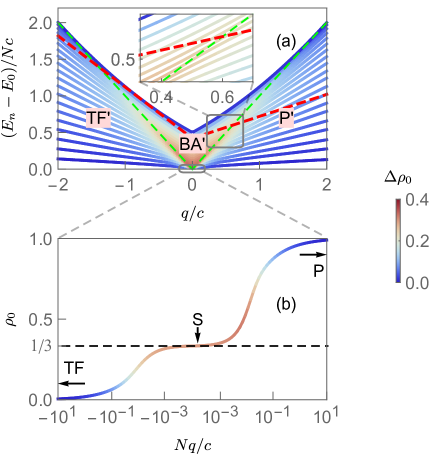
Figure 1: Quantum phases of an antiferromagnetic spin-1 BEC of $N=300$ atoms with zero magnetization, using the number variance $\Delta\rho_{0}$ in spin-0 component. (a) Excited spectra with every $15$ eigenvalues. The green-dashed lines are the ESQPT lines. The red-dashed lines represent the mean-field energy $\mathcal{E}$ of a CSS (4) with $\rho_{0}=0.7$. (b) Ground state varies with $q$ from TF, S to P.

A sketch of the system phase diagram is given in Fig. 1, which is obtained via exact diagonalization of Hamiltonian (1) with an atom number $N=300$. It will be helpful to rewrite Hamiltonian (1) in a more generic form as $\hat{H}=\hat{H}_{0}+q\hat{H}_{q}$, and ground state properties can be recognized as results aroused by the competition between $\hat{H}_{0}$ and $\hat{H}_{q}$: (i) For $\left|q\right|>>c$, the ground state is dominated by $\hat{H}_{q}=\hat{N}_{0}$, thus resulting in Polar (P) state and Twin-Fock (TF) state, with $\rho_{0}\equiv\frac{\left\langle\hat{N}_{0}\right\rangle}{N}=1$ and $0$ respectively, in the positive and negative $q$ direction, associated with vanishing variance $\Delta\rho_{0}\equiv\frac{\Delta\hat{N}_{0}}{N}$; (ii) $\hat{H}_{0}\propto\hat{S}^{2}$ restores SO(3) symmetry in a narrow window of $\left|q\right|<\frac{c}{N^{2}}$, resulting in S ground state with $S=0$ for even $N$. State S is massively entangled typical of large variance $\Delta\rho_{0}$, and with atoms evenly distributed among the magnetic sublevels, representing a three-fragment mesoscopic quantum state with $\rho_{0}=\frac{1}{3}$. In the thermodynamical limit (TL) of $N\rightarrow\infty$, the S state disappears and the QPT is characterized by a 1st-order phase transition between the P and TF state.

The excited eigenspectra display a cumulation of avoided crossings along $E=E_{g}+\left|q\right|$ (green-dashed lines in Fig. 1(a), see the inset for a enlarged view), which correspond to singularities in the density of states under TL. Thus we refer the lines as the ESQPT lines and the variances $\Delta\rho_{0}$ of the eigenstates in the vicinity of these lines also achieve maximum values. The three phases separated by these lines are labled as P^′, TF^′ and BA^′ (broken-axisymmetry). While P^′ and TF^′ are named according to the corresponding ground states, BA^′ is named after the highest energy BA state Sadler et al. (2006); Murata et al. (2007), which possesses a transverse magnetization perpendicular to the applied external field and thus breaks the SO(2) axisymmetry.

DPT and the QFI.— To explore the relation with equilibrium phase transitions, we characterize DPTs with the QFI, which is defined as the fidelity susceptibility Braunstein and Caves (1994); Pang and Brun (2014); Guan and Lewis-Swan (2021)

$$F_{Q}\left(q,t\right)=-4\frac{\partial^{2}F\left(q,\delta q,t\right)}{\partial\left(\delta q\right)^{2}}\Big{|}_{\delta q\rightarrow 0},$$ (2)

where the fidelity $F\left(q,\delta q,t\right)\equiv\left|\left\langle\psi\left(q,t\right)|\psi\left(q+\delta q,t\right)\right\rangle\right|=|\langle\psi_{0}|e^{i\hat{H}\left(q\right)t}e^{-i\hat{H}\left(q+\delta q\right)t}|\psi_{0}\rangle|$ is actually the Loschmidt echo, and it measures the revival of a state $\left|\psi_{0}\right\rangle$ experiencing time forward propagation under $\hat{H}\left(q\right)$ followed by reversed evolution with $\hat{H}\left(q+\delta q\right)$. One can expect that when the system becomes critical with $q\rightarrow q_{c}$, the quantum state evolution behaves singularly and exhibits quite distinct results even for a small $\delta q$, resulting in prominent decrease of the fidelity and a high $F_{Q}$. An approximate long-time secular analytic expression for the QFI can be found as sm

$$F_{Q}\left(q,t\right)\simeq 4t^{2}\left[\sum_{n}\left|c_{n}\right|^{2}\left(H_{q}^{n}\right)^{2}-\left(\sum_{n}\left|c_{n}\right|^{2}H_{q}^{n}\right)^{2}\right],$$ (3)

where $c_{n}=\left\langle\psi_{n}|\psi_{0}\right\rangle$ is the projection of the initial state $\left|\psi_{0}\right\rangle$ onto the eigenstates $\left|\psi_{n}\right\rangle$ of the Hamiltonian (1), and $H_{q}^{n}=\langle\psi_{n}|\hat{H}_{q}|\psi_{n}\rangle$. Equation (3) indicates that a peak in the QFI can be attributed to either enhanced fluctuations in the order parameter ($H_{q}^{n}=N_{0}^{n}=\langle\psi_{n}|\hat{N}_{0}|\psi_{n}\rangle$), or those in the overlaps between the initial state and the eigenstates.

To achieve the correspondence between DPTs and equilibrium phase transitions, one would expect that the overlap between the initial state and system eigenstates $\left|c_{n}\right|^{2}$ has similar singular distribution as the order parameter around the energy $E_{n}^{c}$. We propose to use coherent spin state (CSS) $\left|\zeta\right\rangle^{\otimes N}$ as the initial state, with $\left|\zeta\right\rangle\equiv\sum_{m}\zeta_{m}\left|m\right\rangle$ and $\zeta=\left(\sqrt{\frac{1-\rho_{0}+\rho_{m}}{2}}e^{i\chi_{+}},\sqrt{\rho_{0}},\sqrt{\frac{1-\rho_{0}-\rho_{m}}{2}}e^{i\chi_{-}}\right)^{T}$, where $\rho_{m}=\frac{N_{1}-N_{-1}}{N}$, $\chi_{\pm}=\frac{\theta_{s}\pm\theta_{m}}{2}$ with $\theta_{s\left(m\right)}$ the spinor phase and magnetization phase respectively. CSS can be visualized by casting the corresponding mean-field phase diagram at different $q$ into the spin-nematic phase sphere $\{S_{\perp}\text{, }Q_{\perp}\text{, }2\rho_{0}-1\}$ with the transverse spin $S_{\perp}=\sqrt{\left\langle\hat{S}_{x}\right\rangle^{2}+\left\langle\hat{S}_{y}\right\rangle^{2}}$ and transverse off-diagonal nematic moment $Q_{\perp}=\sqrt{\left\langle\hat{Q}_{xz}\right\rangle^{2}+\left\langle\hat{Q}_{yz}\right\rangle^{2}}$ Hoang et al. (2013), where the quadrapole operators $\hat{Q}_{ij}\equiv\hat{a}_{\alpha}^{\dagger}\left[S_{i}S_{j}+S_{j}S_{i}-\left(4/3\right)\delta_{ij}\right]\hat{a}_{\beta}$ (the indices $\alpha$, $\beta$ are summed over $m$). In the TL, the dynamics of an initial CSS is characterized by its equal-energy trajectories of the spin-nematic component on the sphere. As shown in Fig. 2(a), on the positive $q$ side it can be tuned from that in the P^′ phase space (white line), separatrix dividing the BA^′ and P^′ phase space (red line linked to the unstable hyperbolic point $n_{0}=0$), and that in the BA^′ phase space (yellow line). Similar transitions from BA^′ to TF^′ phase can take place at $q<0$. The spin dynamics can be denoted as coherent oscillation with varying amplitude and period, while for a CSS which is initially localized at the separatrix, it will become singular with diverging period Zhang et al. (2005).

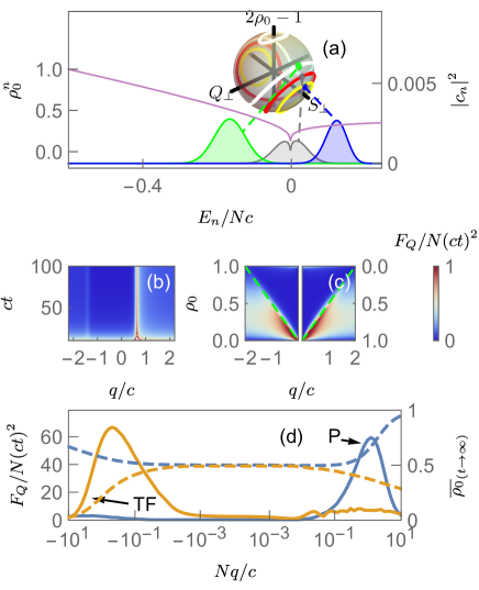
Figure 2: (a) Slice of the phase diagram Fig. 1 at $q=0.6c$ casted into the $\{S_{\perp}$, $Q_{\perp}$, $2\rho_{0}-1\}$ spin-nematic sphere, where the separatrix ($\mathcal{E}=\mathcal{E}_{c}$, red line) separates trajectories in the BA^′ phase ($\mathcal{E}>\mathcal{E}_{c}$, yellow) from those in the P^′ phase ($\mathcal{E}<\mathcal{E}_{c}$, white), and a distribution (the blue, gray, and green circle) represents a CSS on the sphere with $\rho_{0}=0.6,0.7,0.8$ respectively. Eigenstate overlap $\left|c_{n}\right|^{2}$ with these CSSs are plotted (right axis), associated with the Eigenstate normalized population $\rho_{0}^{n}$ (left axis, purple curve). (b) Time evolution of the QFI $F_{Q}$ as a function of $q$. (c) Phase diagram in the $q$-$\rho_{0}$ plane computed with $F_{Q}$ at $ct=10^{3}$. Green-dashed curves refer to ESQPT lines. (d) $F_{Q}$ calculated at $ct=10^{3}$ versus $q$ (left axis) with an initial P state (blue curve), and an initial TF state (brown curve). The corresponding dashed curves represent time-averaged population in spin-0 component $\overline{\rho_{0}\left(t\right)}|_{t\rightarrow\infty}$ (right axis).

Taking the CSS with $\left\{\rho_{0}=0.7\text{, }\rho_{m}=0\text{, }\theta_{s}=\theta_{m}=0\right\}$ as an example (whose mean-field energy $\mathcal{E}$ is shown as the red-dashed line in Fig. 1(a)), at the intersections with the ESQPT line on $q=0.6c$ ($\mathcal{E}=\mathcal{E}_{c}=E_{n}^{c}|_{N\rightarrow\infty}$), for a finite system it represents a distribution on the surface of the spin-nematic sphere with uncertainty equal to SQL ($1/\sqrt{N}$) and center located on the separatrix, which is marked as a gray circle in Fig. 2(a). Since the mean-field energy of the CSS equals that of the critical saddle point, it is closer to the eigenstate at which ESQPT takes place as compared with other higher (blue circle for $\rho_{0}=0.6$) or lower energy CSS (green circle for $\rho_{0}=0.8$), resulting in the nonanalytical features of $\left|c_{n}\right|^{2}$ at $E_{n}^{c}$ (gray line), which are not captured by other SSSs in the P^′ or BA^′ phase (green line and blue line).

We use the CSS as the initial state to simulate QFI (2) with atom number $N=1000$ sm and present the dynamical behavior of $F_{Q}/N\left(ct\right)^{2}$ versus $q$ in Fig. 2(b), where the normalization with respect to $t^{2}$ is chosen to absorb the expected long-time growth of $F_{Q}\propto t^{2}$. Around the critical points $q_{c}=-1.4c$ and $0.6c$, a prominent increase in the QFI can be observed, which correspond to the cases where the CSS is centered on the separatrix, linked to the saddle point $\rho_{0}=1$ and $\rho_{0}=0$, respectively. This suggests that the quantum dynamics exhibits abrupt change around the critical points and thus the QFI can serve as an indicator of ESQPTs. These two QFI peaks in the long-time limit separate the parameter space into three regions, i.e., the BA^′, TF^′, and P^′ phase, respectively. Apart from the phase transition region, the QFI displays damped oscillations.

Motivated by the feasibility that ESQPTs can be distinguished via the QFI, we map out the excited-state phase diagram by varying the initial CSS. One simple choice is that keep $\rho_{m}=0$, $\theta_{s}=\theta_{m}=0$ while vary the value of $\rho_{0}$. For such a state the ESQPT lines display a monotonic relation with $\rho_{0}$ as $q_{c}=2\left(1-\rho_{0}\right)$ in the positive $q$ region and $q_{c}=-2\rho_{0}$ in the negative $q$ region. The preparation of such a CSS can be described by the formula

$$\left|\zeta\right\rangle_{\text{initial}}^{\otimes N}=\frac{1}{\sqrt{N!}}\left(e^{i\frac{\theta}{2}\hat{Q}_{yz}}\hat{a}_{0}^{\dagger}e^{-i\frac{\theta}{2}\hat{Q}_{yz}}\right)^{N}\left|\text{vac}\right\rangle,$$ (4)

with $\cos\theta=\sqrt{\rho_{0}}$ and $\sin\theta=\sqrt{1-\rho_{0}}$. In experiments, Eq. (4) corresponds to a process in which one could first prepare the atoms in the $m=0$ hyperfine state and then apply a combination of magnetic field ramps and resonant radio-frequency (rf) pulses Evrard et al. (2021b) to implement polar state rotation using the quadrapole operator $\hat{Q}_{yz}$. Using the value of $F_{Q}$ in the long time limit at $ct=10^{3}$, the excited-state phase diagram is mapped out in the $q$-$\rho_{0}$ plane, as shown in Fig. 2(c). The vertical axis of $\rho_{0}$ is reversed in the right half ($q>0$) with respect to the left half ($q<0$) in order to make a comparison with the phase diagram in Fig. 1(a). The jump discontinuities signaling the ESQPTs (green dashed lines) can be well captured. One can also notice that the QFI in the vicinity of $\left|q\right|=2c$ is typically much smaller than that around $q=0$, which can be traced to the properties of variance $\Delta\rho_{0}$ calculated in Fig. 1(a).

As for the DPT in ground states, the QFI in the long time limit is calculated with initial P or TF state respectively, which turns out to display a peak value at $q\simeq\pm c/N$, as shown in Fig. 2(d). These QFI peaks correspond to the QPTs of P$\rightarrow$S and TF$\rightarrow$S. For the time-averaged order parameter $\overline{\rho_{0}\left(t\right)}|_{t\rightarrow\infty}\equiv\lim_{T\rightarrow\infty}\frac{1}{T}\int_{0}^{T}\rho_{0}\left(t\right)dt=\sum_{n}\left|c_{n}\right|^{2}N_{0}^{n}/N$, shown as the dashed lines, they donot display any nonanalyticity for the present small size mesoscopic quantum system.

$q$-estimation.—Despite that in principle the QFI can be measured via performing many-body quantum state tomography, or measure the excitation rate of a quantum state upon a periodic drive Ozawa and Goldman (2018, 2019); Yu et al. (2022), it would be complex to implement for a quantum system of hundreds of atoms Evrard et al. (2021a), and the requirement of real-time measure further prevents the feasibility of direct derivation of the QFI. In the estimation theory, the QFI sets the upper bound on the sensitivity of parameter estimation, i.e., $\Delta q\geq 1/\sqrt{F_{Q}\left(q,t\right)}$, which is termed as the quantum Cramér-Rao bound Braunstein and Caves (1994). Thus one can get access to the estimation precision $\left(\Delta q\right)^{-2}$ through an observable $\hat{\mathcal{O}}$ as

$$\left(\Delta q\right)_{\hat{\mathcal{O}}}^{-2}=\frac{\left|\partial_{q}\left\langle\hat{\mathcal{O}}\right\rangle\right|^{2}}{\Delta^{2}\hat{\mathcal{O}}}\leq F_{Q},$$ (5)

with $\Delta^{2}\hat{\mathcal{O}}=\left\langle\hat{\mathcal{O}}^{2}\right\rangle-\left\langle\hat{\mathcal{O}}\right\rangle^{2}$ representing the variance with respect to the initial state $\left|\psi_{0}\right\rangle$. Eq. (5) indicates that the value of $\left(\Delta q\right)_{\hat{\mathcal{O}}}^{-2}$ can approach $F_{Q}$ with an appropriately chosen observable. SQL corresponds to $\left(\Delta q\right)_{\text{SQL}}^{-2}=Nt^{2}$.

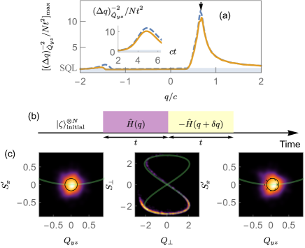
Figure 3: (a) Maximum of the normalized estimation precision $\left(\Delta q\right)_{\hat{Q}_{yz}}^{-2}$ over time as a function of $q$. The arrow indicates the precision peak around $q\simeq 0.67c$, with the corresponding time evolution shown in the inset. The dashed lines are those for the QFI, which set the upper bound of the precision. (b) Schematic showing the protocol of echo for parameter estimation. (c) Density plot from the TWA simulation on the inset of (a), where time is chosen to be that the optimal precision is achieved, at $ct\simeq 4.88$. The scale is taken to be $100$ atoms and the separatrix is shown in green curve. Left panel: Distribution of the initial CSS on the $S_{x}^{\prime}$-$Q_{yz}$ space with uncertainty ellipse shown in black curve. Middle panel: Distribution on the $S_{\perp}$-$Q_{\perp}$ space after the time-forward propagation. Right panel: Distribution at the end of the echo. The uncertainty ellipse (black solid curve) shifts in the $Q_{yz}$-direction as compared with that of the initial state (black dotted curve). All calculations are for $N=300$.

Considering that optimal precision is more likely to be achieved for an observable with small variance, instead of the order parameter $\hat{N}_{0}$, we propose to use the quadrapole operator $\hat{Q}_{yz}$ as the observable (note that $\hat{Q}_{yz}$ is also found to determine the best precision in a spin-1 condensate interferometry Niezgoda et al. (2019)). While $\hat{S}_{x}$ and $\hat{Q}_{yz}$ construct a pair of observables exhibiting spin-nematic squeezing for an initial P state Hamley et al. (2012), $\hat{S}_{x}^{\prime}=\exp\left(i\frac{\theta}{2}\hat{Q}_{yz}\right)\hat{S}_{x}\exp\left(-i\frac{\theta}{2}\hat{Q}_{yz}\right)$ and $\hat{Q}_{yz}$ are those for the CSS (4) through a unitary transformation Yukawa et al. (2013). The initial state then constitutes a minimum uncertainty state for $\hat{S}_{x}^{\prime}$ and $\hat{Q}_{yz}$, as shown in the left panel of Fig. 3(c). In experiment $Q_{yz}=\left\langle\hat{Q}_{yz}\right\rangle$ can be measured via first exchanging the distribution of $Q_{yz}$ with that along $S_{x}$ using microwave pulse, then applying a $\frac{\pi}{2}$ rf rotation about $S_{y}$ and performing Stern-Gerlach gradient imaging Hamley et al. (2012). Similar to the definition of the QFI in (2), the precision estimation also invokes an echo process, which is illustrated in Fig. 3(b). We use truncated Wigner approximation (TWA) to derive the variation of $Q_{yz}$ after the echo sm , from which the maximum values of $\left(\Delta q\right)_{\hat{Q}_{yz}}^{-2}$ are found and they synchronize well with the behavior of $F_{Q}$, as shown in Fig. 3(a). Same as Fig. 2(b), here we also take the CSS (4) with $\rho_{0}=0.7$ as the initial state. A small deviation between the peaks of $\left(\Delta q\right)_{\hat{Q}_{yz}}^{-2}$ and the mean-field prediction exists, as indicated by the arrow, where the peak locate around $q\simeq 0.67c$ instead of the mean-field critical value of $q_{c}=0.6c$, and this can be attributed to the transient and finite-size effects.

To understand the physics beneath the enhanced sensing, we explore the echo process during which $\left(\Delta q\right)_{\hat{Q}_{yz}}^{-2}$ reaches its peak value (the inset of Fig. 3(a)). After a time-forward evolution under $\hat{H}\left(q\right)$, the atomic state is dispersed along the separatrix, with its majority surpassing the saddle point, as shown in the middle panel of Fig. 3(c). Noticeably that part of the quasi-probability distribution even leaves the separatrix and enters into the P^′ phase space. This is due to that the motion near the separatrix is apt to phase space mixing Mathew and Tiesinga (2017). At the end of the echo after experiencing a time-reversing evolution under $\hat{H}\left(q+\delta q\right)$, the state approximately recovers the initial CSS (right panel of Fig. 3(c)), with a small shift in the $Q_{yz}$ component (compare the uncertainty ellipse of initial and final states, marked by dotted and solid line respectively). A small perturbation in the control parameter ($\delta q=10^{-3}c$ in Fig. 3(c)) can give rise to non-negligible variation in the observable, and this roots in the sensitive dependence of quantum state evolution upon the deformation of the separatrix, which is well captured through an echo process near the critical points.

Conclusion.—In summary, we have shown the existence of QPTs and ESQPTs in an antiferromagnetic spin-1 condensate and demonstrated their correspondence with DPT, which is characterized using the QFI. We propose that DPT with the condensate initially prepared in an CSS can be used to probe the quantum criticality in excited states, which gives rise to a peak value of the QFI. It can also be used to implement sub-SQL estimation on the effective quadratic Zeeman energy $q$. This extends the precise estimation of the critical $q_{c}$ to a much wider parameter region beyond those at which ground state QPTs take place Mirkhalaf et al. (2020, 2021). It is interesting to note that the ground-state phase transitions from symmetry-broken states to the symmetry-restored spin-singlet state can also be indicated by the DPT. Though we have focused on the system of spinor condensate, the method of exploring ESQPTs presented here can be applied to a broad class of few-mode quantum systems.

I numerical methods

We solve the time evolution of quantum states using the exact diagonalization method. The initial state of the system is described by a coherent spin state $\left|\zeta\right\rangle^{\otimes N}$ with (assuming $\rho_{+1}=\rho_{-1}$)

$$\zeta=\left(\begin{array}[]{c}\zeta_{+1}\\ \zeta_{0}\\ \zeta_{-1}\end{array}\right)=\left(\begin{array}[]{c}\sqrt{\frac{1-\rho_{0}}{2}}e^{i\phi_{+1}}\\ \sqrt{\rho_{0}}e^{i\phi_{0}}\\ \sqrt{\frac{1-\rho_{0}}{2}}e^{i\phi_{-1}}\end{array}\right),$$ (S1)

where equal population in the spin-$\pm 1$ sublevels is assumed. $\left|\zeta\right\rangle^{\otimes N}$ can be written in the Fock basis as

$$\left|\zeta\right\rangle^{\otimes N}=\frac{1}{\sqrt{N!}}\left(\zeta_{+1}\hat{a}_{+1}^{\dagger}+\zeta_{0}\hat{a}_{0}^{\dagger}+\zeta_{-1}\hat{a}_{-1}^{\dagger}\right)^{N}\left|0\right\rangle,$$ (S2)

which can be expanded in the Fock basis $\left|N_{0},M\right\rangle\equiv\left|N_{1}=\frac{N-N_{0}+M}{2},N_{0},N_{-1}=\frac{N-N_{0}-M}{2}\right\rangle$ as $\left|\zeta\right\rangle^{\otimes N}=\sum_{N_{0},M}f\left(N_{0},M\right)\left|N_{0},M\right\rangle$ with the coefficient

$$f\left(N_{0},M\right)=\sqrt{\frac{N!}{N_{1}!N_{0}!N_{-1}!}}\left(\sqrt{\frac{1-\rho_{0}}{2}}\right)^{N-N_{0}}\left(\sqrt{\rho_{0}}\right)^{N_{0}}\exp\left[i\left(N_{1}\phi_{+1}+N_{0}\phi_{0}+N_{-1}\phi_{-1}\right)\right].$$ (S3)

Due to the presence of the SO(2) symmetry in the Hamiltonian (1) spinorsymmetry-s , the generator $\hat{S}_{z}$ is conserved, i.e., the magnetization $M$ is a conserved quantity. Then the Hamiltonian matrix $\hat{H}$ written in the $\left|N_{0},M\right\rangle$ basis is block diagonal, for which there are $2N+1$ blocks with the value of $M$ running from $-N$ to $N$ and each block has a dimension $\left[\frac{N-M}{2}+1\right]\times\left[\frac{N-M}{2}+1\right]$ (here $\left[\cdot\right]$ means taking the integer part). Each block matrix is tridiagonal and can be diagonalized separately, then the time evolved state $\left|\psi\left(q,t\right)\right\rangle$ can be computed.

Some spin operators such as $\hat{Q}_{yz}$ couples blocks of different $M$, which makes its matrix size very large and inconvenient to perform simulation. We adopt TWA to study its dynamics twa1-s ; twa2-s ; twa3-s ; twa5-s . TWA states that the Wigner function $W$ for a quantum state approximately follows the equation

$$i\hbar\frac{\partial W}{\partial t}\simeq\left\{H_{W},W\right\}_{C},$$ (S4)

where $H_{W}$ is the Wigner-Weyl transform of the Hamiltonian, and $\left\{\cdots\right\}_{C}$ is the coherent state Poisson bracket. Similarly in the coherent state picture we treat the operators $\hat{a}_{j}$ ($\hat{a}_{j}^{\dagger}$) as complex $c$-numbers $\alpha_{j}$ ($\alpha_{j}^{\ast}$), and making Wigner-Weyl transform to the Heisenberg equations we have

$$i\hbar\frac{\partial\alpha_{j}}{\partial t}\simeq\left\{\alpha_{j},H_{W}\right\}_{C}=\frac{\partial H_{W}}{\partial\alpha_{j}^{\ast}}.$$ (S5)

TWA then invokes first sampling the Wigner distribution $W$ with many sets of $\left\{\alpha_{j},\alpha_{j}^{\ast}\right\}$, and then for each set we solve the equation of motion (S5). Any observable of interest is obtained from the ensemble average. To sample $\left|\zeta\right\rangle^{\otimes N}$, we first sample the polar state $\frac{1}{\sqrt{N!}}\hat{a}_{0}^{\dagger N}\left|\text{vac}\right\rangle$ with

$$\left(\begin{array}[]{c}\alpha_{1}\\ \alpha_{0}\\ \alpha_{-1}\end{array}\right)=\left(\begin{array}[]{c}\left(a+ib\right)/2\\ \left(e+f\eta\right)e^{i2\pi\xi}\\ \left(c+id\right)/2\end{array}\right),$$ (S6)

where $a,b,c,d,\eta$ are independent random numbers drawn from Gaussian distribution with zero mean and unit variance, while $\xi$ is a random number drawn from uniform distribution in $\left[0,1\right]$, and wignersample-s

$$e=\frac{1}{2}\sqrt{2N+1+2\sqrt{N^{2}+N}},f=\frac{1}{4e}.$$ (S7)

Unitary transformation (4) is equivalent to performing the rotation

$$\left(\begin{array}[]{ccc}\frac{\cos\theta+1}{2}&\frac{\sin\theta}{\sqrt{2}}&\frac{\cos\theta-1}{2}\\ -\frac{\sin\theta}{\sqrt{2}}&\cos\theta&-\frac{\sin\theta}{\sqrt{2}}\\ \frac{\cos\theta-1}{2}&\frac{\sin\theta}{\sqrt{2}}&\frac{\cos\theta+1}{2}\end{array}\right)\left(\begin{array}[]{c}\alpha_{1}\\ \alpha_{0}\\ \alpha_{-1}\end{array}\right).$$ (S8)

We sample a system of $N=300$ with $1000$ trajectories. It has been compared with the exact quantum mechanical calculations regarding the expectation values and variances of different spin operators, where good agreements are found. TWA is capable to simulate quantum dynamics in short time scale, which is enough for us to produce Fig. 3. However it will deviate significantly from the exact quantum mechanical calculations when the evolution time becomes large, due to the omitted high-order terms.

II secular approximation of the QFI

The QFI (2) can be written in a tensor form as qfitensor-s

$$F_{Q}\left(q,t\right)=4\left(\left\langle\partial_{q}\psi|\partial_{q}\psi\right\rangle-\left|\left\langle\psi|\partial_{q}\psi\right\rangle\right|^{2}\right),$$ (S9)

where $\left|\psi\right\rangle=\left|\psi\left(q,t\right)\right\rangle=e^{-i\hat{H}t}\left|\psi_{0}\right\rangle$. If $\hat{H}=q\hat{H}_{q}$, one can immediately realize that $F_{Q}\left(q,t\right)=4t^{2}\Delta^{2}\hat{H}_{q}$ with the variance $\Delta^{2}\hat{H}_{q}=\left\langle\psi_{0}\left|\hat{H}_{q}^{2}\right|\psi_{0}\right\rangle-\left|\left\langle\psi_{0}\left|\hat{H}_{q}\right|\psi_{0}\right\rangle\right|^{2}$. Recognizing $\hat{H}=\hat{H}_{0}+q\hat{H}_{q}$ and $\left[\hat{H}_{0},\hat{H}_{q}\right]\neq 0$, we use the identity deo-s

$$\exp\left(i\hat{H}t\right)\frac{\partial}{\partial q}\exp\left(-i\hat{H}t\right)=-i\int_{0}^{t}dt^{\prime}\exp\left(i\hat{H}t^{\prime}\right)\frac{\partial\hat{H}}{\partial q}\exp\left(-i\hat{H}t^{\prime}\right)=-i\mathcal{\hat{H}}_{q},$$ (S10)

where $\mathcal{\hat{H}}_{q}=\int_{0}^{t}dt^{\prime}\exp\left(i\hat{H}t^{\prime}\right)\hat{H}_{q}\exp\left(-i\hat{H}t^{\prime}\right)$ and this leads to $F_{Q}\left(q,t\right)=4\Delta^{2}\hat{\mathcal{H}}_{q}$. Usually, it is not easy to work out the explicit form of $\hat{\mathcal{H}}_{q}$ except that the Hamiltonian belongs to some special classes caiprl2021-s . Using the expansion $\left|\psi_{0}\right\rangle=\sum_{n}c_{n}\left|\psi_{n}\right\rangle$, in which $\left|\psi_{n}\right\rangle$ is the eigenstate of $\hat{H}$ with the corresponding eigenenergy $E_{n}$, we can get

$$F_{Q}\left(q,t\right)=4t^{2}\left[\sum_{n}\left|\sum_{m}c_{m}H_{q}^{nm}\text{sinc}\left(\frac{E_{nm}t}{2}\right)e^{iE_{nm}t/2}\right|^{2}-\left|\sum_{n,m}c_{n}^{\ast}c_{m}H_{q}^{nm}\text{sinc}\left(\frac{E_{nm}t}{2}\right)e^{iE_{nm}t/2}\right|^{2}\right],$$ (S11)

where $E_{nm}=E_{n}-E_{m}$. In the long-time limit, the sinc function gives the value of $1$ with $E_{nm}=0$ and zero otherwise. Using an assumption that only the terms with $E_{nm}=0$ survive in the $t\rightarrow\infty$ limit dynamicalqfi-s  and considering the fact that the spectrum of $\hat{H}$ is nondegenerate, the QFI (S11) can be approximated by Eq. (3) in the main text.

We found out that the approximation is quantitatively valid in a moderate long time. From the viewpoint of phase space mixing phasespacemixing-s , a distribution in phase space will eventually mix up in the energy region it could reach, which will reduce its distinguishability. The sensitivity of a quantum state with respect to the change of Hamiltonian parameters, as characterized by the QFI, is also expected to become coarse in the long-time run.

III experimental consideration

The echo including first evolves an initial state $\left|\psi_{0}\right\rangle$ forward with $\hat{H}\left(q\right)$ and then backward with $\hat{H}\left(q+\delta q\right)$. To implement this, one needs to reverse the sign of the Hamiltonian $\hat{H}=\hat{H}_{0}+q\hat{H}_{q}$ such that the system can experience time-reversing evolution. In experiments, the sign of the control parameter $q$ can be varied via microwave dressing qsignreverse-s ; microwave1-s ; microwave2-s . On the other hand, the sign of $\hat{H}_{0}$ is determined by the spin-dependent interaction coefficient $c$, which may be reversed via transferring the atoms from the $F=1$ hyperfine manifold to that of $F=2$ oberthalerPRL2019-s . Another promising technique could be exploited is the photon-mediated spin-exchange interactions, which was experimentally realized recently with the aid of a cavity light field signreverse-s ; lmgscience-s . Other methods capable of manipulating spin-dependent collision interactions, such as photoassociation jinghuiphotoassociation-s , also exist.

References

- (1) Y. Kawaguchi and M. Ueda, Symmetry classification of spinor Bose-Einstein condensates, Phys. Rev. A 84, 053616 (2011).
- (2) P. B. Blakie, A. S. Bradley, M. J. Davis, R. J. Ballagh, and C. W. Gardiner, Dynamics and statistical mechanics of ultra-cold Bose gases using c-field techniques, Adv. Phys. 57, 363 (2008).
- (3) A. Polkovnikov, Phase space representation of quantum dynamics, Ann. Phys. 325, 1790 (2010).
- (4) J. Schachenmayer, A. Pikovski, and A. M. Rey, Many-Body Quantum Spin Dynamics with Monte Carlo Trajectories on a Discrete Phase Space, Phys. Rev. X 5, 011022 (2015).
- (5) A. Sinatra, C. Lobo and Y. Castin, The truncated Wigner method for Bose-condensed gases: limits of validity and applications, J. Phys. B 35, 3599 (2002).
- (6) M. K. Olsen and A. S. Bradley, Numerical representation of quantum states in the positive- and Wigner representations, Opt. Comm. 282, 3924 (2009).
- (7) L. C. Venuti and P. Zanardi, Quantum Critical Scaling of the Geometric Tensors, Phys. Rev. Lett. 99, 095701 (2007).
- (8) R. M. Wilcox, Exponential Operators and Parameter Differentiation in Quantum Physics, J. Math. Phys. 8, 962 (1967).
- (9) Y. Chu, S. Zhang, B. Yu, and J. Cai, Dynamic Framework for Criticality-Enhanced Quantum Sensing, Phys. Rev. Lett. 126, 010502 (2021).
- (10) Q. Guan and R. J. Lewis-Swan, Identifying and harnessing dynamical phase transitions for quantum-enhanced sensing, Phys. Rev. Research 3, 033199 (2021).
- (11) R. Mathew and E. Tiesinga, Phase-space mixing in dynamically unstable, integrable few-mode quantum systems, Phys. Rev. A 96, 013604 (2017).
- (12) P. Kunkel, M. Prüfer, H. Strobel, D. Linnemann, A. Frölian, T. Gasenzer, M. Gärttner, and M. K. Oberthaler, Spatially distributed multipartite entanglement enables EPR steering of atomic clouds, Science 360, 413 (2018).
- (13) F. Gerbier, A. Widera, S. Fölling, O. Mandel, and I. Bloch, Resonant control of spin dynamics in ultracold quantum gases by microwave dressing, Phys. Rev. A 73, 041602 (2006).
- (14) S. R. Leslie, J. Guzman, M. Vengalattore, J. D. Sau, M. L. Cohen, and D. M. Stamper-Kurn, Amplification of fluctuations in a spinor Bose-Einstein condensate, Phys. Rev. A 79, 043631 (2009).
- (15) P. Kunkel, M. Prüfer, S. Lannig, R. Rosa-Medina, A. Bonnin, M. Gärttner, H. Strobel, and M. K. Oberthaler, Simultaneous Readout of Noncommuting Collective Spin Observables beyond the Standard Quantum Limit, Phys. Rev. Lett. 123, 063603 (2019).
- (16) E. J. Davis, G. Bentsen, L. Homeier, T. Li, and M. H. Schleier-Smith, Photon-Mediated Spin-Exchange Dynamics of Spin-1 Atoms, Phys. Rev. Lett. 122, 010405 (2019).
- (17) M. A. Norcia, R. J. Lewis-Swan, J. R. K. Cline, B. Zhu, A. M. Rey, and J. K. Thompson, Cavity-mediated collective spin-exchange interactions in a strontium superradiant laser, Science 361, 259 (2018).
- (18) H. Jing, Y. Jiang, W. Zhang, and P. Meystre, Laser-catalyzed spin-exchange process in a Bose-Einstein condensate, Phys. Rev. A 81, 031603 (2010).